Hardness of observing strong-to-weak symmetry breaking

Abstract

Spontaneous symmetry breaking (SSB) is the cornerstone of our understanding of quantum phases of matter. Recent works have generalized this concept to the domain of mixed states in open quantum systems, where symmetries can be realized in two distinct ways dubbed strong and weak. Novel intrinsically mixed phases of quantum matter can then be defined by the spontaneous breaking of strong symmetry down to weak symmetry. However, proposed order parameters for strong-to-weak SSB (based on mixed-state fidelities or purities) seem to require exponentially many copies of the state, raising the question: is it possible to efficiently detect strong-to-weak SSB in general? Here we answer this question negatively in the paradigmatic cases of $\mathbb{Z}_{2}$ and $U(1)$ symmetries. We construct ensembles of pseudorandom mixed states that do not break the strong symmetry, yet are computationally indistinguishable from states that do. This rules out the existence of efficient state-agnostic protocols to detect strong-to-weak SSB.

Introduction.—Quantum phases of matter are best understood for ground states of isolated quantum systems, described by pure states Wen (2017). Their robustness to perturbations that cause the state to become mixed (e.g. finite temperature, decoherence) is an interesting fundamental question Dennis et al. (2002); Hastings (2011); Lu et al. (2020); Fan et al. (2024). Recent works have pointed out another interesting possibility: the existence of intrinsically mixed quantum phases of matter, exhibiting patterns of symmetry breaking without a pure-state analogue Lee et al. (2023, 2025); Lessa et al. (2025); Wang et al. (2025); Ellison and Cheng (2025); Sohal and Prem (2025); Zhang et al. (2025); Chen and Grover (2024); Ma et al. (2025); Ma and Turzillo (2025).

This possibility arises because mixed states can realize a symmetry in two physically distinct ways: an exact or strong symmetry, and an average or weak symmetry. Precisely, for a unitary $U$ representing the action of a given symmetry on the Hilbert space, a mixed state $\rho$ has a strong symmetry if $U\rho\propto\rho$, and a weak symmetry if $U\rho U^{\dagger}=\rho$. Both conditions require that $\rho$ can be unraveled into a mixture of symmetric pure states, however strong symmetry also requires all states in the mixture to have the same symmetry charge. This richer structure of symmetries enables a route to SSB that is unique to mixed states, known as strong-to-weak spontaneous symmetry breaking (SWSSB). Many intriguing properties of this phenomenon have been recently investigated in quantum systems at finite temperature or under the effect of local decoherence channels Lee et al. (2023, 2025); Lessa et al. (2025); Wang et al. (2025); Ellison and Cheng (2025); Sohal and Prem (2025); Zhang et al. (2025); Chen and Grover (2024); Ma et al. (2025); Ma and Turzillo (2025); Kuno et al. (2024); Gu et al. (2024a); Zhang et al. (2024); Huang et al. (2025).

In pure states, SSB can be characterized by long range order in the correlation function $\langle O_{i}O_{j}^{\dagger}\rangle$, where $O_{i}$ and $O_{j}$ are local operators that are charged under the global symmetry Sachdev (2011). In contrast, known diagnostics of SWSSB do not take the form of local expectation values; they are instead information-theoretic functions that are nonlinear in the density matrix $\rho$. Such diagnostics include the Rényi-2 correlator Lee et al. (2023); Ma and Turzillo (2025); Sala et al. (2024), the fidelity correlator Lessa et al. (2025); Zhang et al. (2024), and the Rényi-1 (or Wightman) correlator Weinstein (2024); Liu et al. (2024). These present different advantages and disadvantages in terms of analytical tractability, robustness to strongly-symmetric perturbations, etc, but they share a common limitation in terms of experimental access. Indeed, while nonlinearity in $\rho$ is not an issue in and of itself (it can be handled by protocols such as classical shadows Huang et al. (2020); Elben et al. (2023); Sun et al. (2025)), each proposed diagnostic involves the measurement of quantities like mixed-state fidelity and purity which cannot be carried out efficiently in general. Thus, despite specific recent proposals Weinstein (2024); Sun et al. (2025), the experimental observability of SWSSB in general remains an open question.

In this work we conclusively answer this question. We establish that, given copies of a strongly-symmetric density matrix $\rho$ and no additional information, no efficient protocol can decide whether or not $\rho$ exhibits SWSSB in general. We achieve this result by leveraging recent constructions of pseudorandom unitaries (PRUs) Ji et al. (2018); Metger et al. (2024); Ma and Huang (2024); Chen et al. (2024) and pseudorandom density matrices Bansal et al. (2025). Specifically, we construct ensembles of mixed states that do not exhibit SWSSB, yet are computationally indistinguishable from states that do. “Computationally indistinguishable” means that the two ensembles cannot be distinguished by any protocol using resources (time, number of state copies) scaling polynomially in the number of qubits $N$. Since an efficient state-agnostic protocol to detect SWSSB would be able to distinguish the two ensembles, such a protocol cannot exist. Our work thus establishes a fundamental limitation on the observability of intrinsicallly mixed phases of matter.

In the following we present the general idea of “pseudo-SWSSB” state ensembles and their construction for the paradigmatic cases of $\mathbb{Z}_{2}$ and $U(1)$ symmetries.

Pseudo-SWSSB.—SSB in pure states is diagnosed by long-ranged correlations $C(i,j)={\rm Tr}(\rho O_{i}O_{j}^{\dagger})$, with $O_{i}$ a local operator charged under the symmetry group $G$. Such correlations are efficiently measurable in experiment. In contrast, SWSSB in mixed states is described by long-ranged correlations of different types, which may not be easily accessed experimentally. We review three commonly used diagnostics. The Rényi-2 correlator, $R_{2}(i,j):={\Tr\left(\rho O_{i}O_{j}^{\dagger}\rho O_{i}^{\dagger}O_{j}\right)}/{\Tr\rho^{2}}$, requires precise measurement of the purity $\Tr\rho^{2}$, which can be exponentially small leading to an exponentially large sample complexity. The fidelity correlator, defined by $F(i,j):=\Tr\sqrt{\sqrt{\rho}O_{i}O_{j}^{\dagger}\rho O_{i}^{\dagger}O_{j}\sqrt{\rho}}$, is the fidelity between the two mixed states $\rho$ and $O_{i}O_{j}^{\dagger}\rho O_{i}^{\dagger}O_{j}$, whose measurement in general requires exponentially-costly tomography Yuen (2023) (recent work presents a series expansion in terms of Rényi-$2n$ correlators Zhang et al. (2024), which is at least as hard as measuring $R_{2}$). Finally, the Rényi-1 or Wightman correlator $R_{1}(i,j):=\Tr\left(\sqrt{\rho}O_{i}O_{j}^{\dagger}\sqrt{\rho}O_{i}^{\dagger}O_{j}\right)$ can be efficiently measured with knowledge of how to prepare the “canonical purification” state $\sqrt{\rho}$ Weinstein (2024), but in the absence of this information, requires state tomography similarly to $F$.

We say that a state $\rho$ exhibits SWSSB if it is strongly symmetric ($U\rho\propto\rho$) and spontaneously breaks the stron symmetry but not the weak one. The strong symmetry is broken if the Rényi-1 correlator $R_{1}(i,j)$ remains finite in the limit of large spatial separation between the points $i$ and $j$. Similarly, the weak symmetry is unbroken if the standard correlator $C(i,j)={\rm Tr}(\rho O_{i}O_{j}^{\dagger})$ vanishes with increasing distance. We note that $R_{1}$ and $F$ are equivalent for this purpose Liu et al. (2024); Weinstein (2024). On the other hand $R_{2}$ does not enjoy a stability theorem with respect to strongly symmetric quantum channels Lessa et al. (2025), and so may not identify mixed state phases correctly.

With this background, we can now give a definition of pseudo-SWSSB ensembles of mixed states.

Definition 1 (Pseudo-SWSSB).

For a given symmetry group $G$, an ensemble of $N$-qubit density matrices $\mathcal{E}(G)$ exhibits “pseudo-SWSSB” under $G$ if it satisfies the following properties: (i) each state $\rho\in\mathcal{E}(G)$ is efficiently preparable; (ii) each $\rho\in\mathcal{E}(G)$ is strongly symmetric under $G$; (iii) the strong $G$-symmetry is unbroken: $\sum_{i,j}R_{1}(i,j)=o(N^{2})$ with high probability over $\rho\sim\mathcal{E}(G)$ as $N\to\infty$; (iv) the ensemble $\mathcal{E}(G)$ is computationally indistinguishable from a state $\rho_{g}$ that exhibits SWSSB: for any number of copies $k={\rm poly}(N)$ and any efficient quantum algorithm $\mathcal{A}$,

$$\left|\mathcal{A}\left(\rho^{\otimes k}_{g}\right)-\mathcal{A}\left({\mathbb{E}}_{\rho\sim\mathcal{E}(G)}\rho^{\otimes k}\right)\right|\leq o(1/{\rm poly}(N)).$$ (1)

Here a quantum algorithm is a binary measurement with outcomes $0,1$, i.e., $\mathcal{A}(\rho_{g}^{\otimes k})={\rm Tr}(E\rho_{g}^{\otimes k})$ with $0\leq E\leq\mathbb{I}$ an operator on $k$ Hilbert space copies. It is efficient if it can be implemented in ${\rm poly}(N)$ depth with ${\rm poly}(N)$ auxiliary qubits.

Let us remark on the meaning of Definition 1. If there was an efficient algorithm $\mathcal{A}$ capable of diagnosing SWSSB given polynomially many copies of an unknown state $\rho$, then one could use $\mathcal{A}$ to distinguish the ensemble $\mathcal{E}(G)$ from $\rho_{g}^{\otimes k}$—which contradicts the definition of $\mathcal{E}(G)$. Thus the existence of a pseudo-SWSSB ensemble would rule out such an algorithm, establishing a fundamental limitation on the observability of SWSSB. Specifically, it would imply that protocols to detect SWSSB in arbitrary unknown states necessarily require a superpolynomial amount of resources (e.g. state copies). Conversely, efficient protocols to detect SWSSB necessarily require additional assumptions or prior information about the state $\rho$. A protocol in the latter category was proposed in Ref. Weinstein (2024).

Another interesting observation on Definition 1 is that, in point (iii), we do not have to separately ask for the weak symmetry to be unbroken in $\mathcal{E}(G)$: this follows from property (iv) if we pick the efficient algorithm $\mathcal{A}$ that measures $O_{i}O_{j}^{\dagger}\otimes O_{i}^{\dagger}O_{j}$ on $k=2$ state copies, returning $|C(i,j)|^{2}$. Then, since $|C(i,j)|^{2}$ is negligibly small in $\rho_{g}$, the same must be true on average over $\mathcal{E}(G)$, bounding both mean and variance of $C(i,j)$ over the ensemble and showing that the weak symmetry is unbroken. This highlights a key distinction between strong and weak symmetry: it is impossible to hide SSB for the weak symmetry because the order parameter is a polynomial in $\rho$; conversely, since the order parameters for the strong symmetry are not polynomials in $\rho$, the possibility of concealing SSB exists.

In the following we present rigorous constructions of pseudo-SWSSB ensembles for $\mathbb{Z}_{2}$ symmetry and $U(1)$ symmetry, thus establishing the hardness of detecting SWSSB in these paradigmatic cases. Generalization to the less explored case of non-Abelian symmetry is an interesting direction for future work.

$\mathbb{Z}_{2}$ symmetry.—We start by considering an $N$-qubit Hilbert space with a $\mathbb{Z}_{2}$ symmetry generated by $\bar{X}=\prod_{i}X_{i}$, with local charged operators $Z_{i}$ ($\bar{X}Z_{i}\bar{X}=-Z_{i}$). The prototypical SWSSB state in this case is $\rho_{0}=(\mathbb{I}+\bar{X})/d$, where $d=2^{N}$ is the Hilbert space dimension. This is the maximally mixed state in the subspace $\mathcal{H}_{+}$, the $+1$ eigenspace of $\bar{X}$. It is easy to verify that $\bar{X}\rho_{0}=\rho_{0}$ (strong symmetry) and ${\rm Tr}(\rho_{0}Z_{i}Z_{j})=0$ for all $i\neq j$ (unbroken weak symmetry). At the same time, since $Z_{i}Z_{j}\rho_{0}Z_{i}Z_{j}=\rho_{0}$, we have $R_{1}(i,j)=F(i,j)=R_{2}(i,j)=1$ for all $i$ and $j$ (broken strong symmetry).

Before presenting our rigorous construction of the pseudo-SWSSB ensemble, let us qualitatively sketch the main ideas. Consider a stochastic mixture of some number $r$ of independent Haar-random states inside symmetry sector $\mathcal{H}_{+}$: $\rho=r^{-1}\sum_{\alpha=1}^{r}\outerproduct{\psi_{\alpha}}{\psi_{\alpha}}$, where $\bar{X}\ket{\psi_{\alpha}}=+\ket{\psi_{\alpha}}$ for all $\alpha$. Since any two states in the mixture are nearly orthogonal with high probability (if $r$ is not too big), this state has purity ${\rm Tr}(\rho^{2})\approx 1/r$. The Rényi-2 correlator then reads $R_{2}(i,j)\simeq r^{-1}\sum_{\alpha,\beta}|\bra{\psi_{\alpha}}Z_{i}Z_{j}\ket{\psi_{\beta}}|^{2}$. Since the $\ket{\psi_{\alpha}}$ states are Haar-random, the typical value of each matrix element will be $|\langle\psi_{\alpha}|\psi_{\beta}\rangle|^{2}=O(1/d)$, and $R_{2}(i,j)=O(r^{2}/d)$ for all $i\neq j$. If the chosen rank $r$ grows sub-exponentially in $N$, then $\rho$ does not break the strong symmetry, and so does not have SWSSB (at least according to $R_{2}$). Yet if $r$ is large enough, $\rho$ is a highly mixed state in a randomized basis of $\mathcal{H}_{+}$, and so we may expect it to be hard to distinguish from $\rho_{0}$, the maximally mixed state in the subspace, which does have SWSSB. Below we develop this idea into a derandomized construction that is efficiently implementable, and we prove absence of SWSSB according to $R_{1}$ as well as computational indistinguishability from the SWSSB state $\rho_{0}$.

To derandomize our construction, it is essential to make use of pseudorandom unitaries:

Definition 2 (Pseudorandom unitary Ji et al. (2018); Metger et al. (2024); Ma and Huang (2024); Chen et al. (2024)).

A family of ensembles $\{\mathcal{U}_{{\rm PRU},N}\}_{N\in\mathbb{N}}$ of $N$-qubit unitaries is a PRU if (i) each $U\in\mathcal{U}_{{\rm PRU},N}$ is efficiently implemented in depth ${\rm poly}(N)$, and (ii) a unitary chosen uniformly at random from $\mathcal{U}_{{\rm PRU},N}$ is computationally indistinguishable from a Haar-random unitary: any efficient algorithm querying $U$ in parallel $k={\rm poly}(N)$ times gives the same average outcome whether $U$ is a PRU or a Haar-random unitary, up to error $o(1/{\rm poly}(N))$.

In particular we will use the recently introduced ‘PFC’ ensemble Metger et al. (2024), where each $U$ is the composition of a pseudorandom permutation of the computational basis Zhandry (2025), a pseudorandom binary phase function Zhandry (2021), and a random Clifford unitary van den Berg (2021). This has the advantage of additionally forming an exact 2-design Ambainis and Emerson (2007); Dankert et al. (2009); Roberts and Yoshida (2017), due to the random Clifford.

We define our pseudo-SWSSB ensemble as

$$\mathcal{E}(\mathbb{Z}_{2}):=\left\{\frac{U\Pi_{r}U^{\dagger}}{r}:\ U\sim\mathcal{U}_{\rm PRU}(\mathcal{H}_{+})\right\},$$ (2)

with $\Pi_{r}$ a rank-$r$ projector supported inside the symmetry sector subspace $\mathcal{H}_{+}$ and $\mathcal{U}_{\rm PRU}(\mathcal{H}_{+})$ a PRU ensemble on $\mathcal{H}_{+}$. These states can be prepared efficiently. A possible approach, illustrated in Fig. 1(a), is to take a product state $\ket{+}\otimes\ket{0}^{\otimes N-1}$ and apply a fully depolarizing channel to the last $\log_{2}(r)$ qubits (we can assume $r$ is a power of 2) to get a mixed state with the desired spectrum; then we apply a PRU on qubits $i=2,\dots N$; finally we apply the encoder circuit for the repetition code where qubit $i=1$ serves as the ‘logical’ and qubits $i=2,\dots N$ as the ‘syndromes’. The encoder circuit turns $X_{1}$ into the global symmetry operator $\bar{X}$, which ensures the output state is within the $\bar{X}=+1$ sector since the input has $X_{1}=+1$. In all, this results in a state $U\Pi_{r}U^{\dagger}/r$ with $U$ a PRU on the symmetry sector subspace $\mathcal{H}_{+}$. The state can be prepared efficiently since the repetition code encoder is implementable as a depth-$N$ staircase of CNOT gates and PRUs are efficiently implementable by definition.

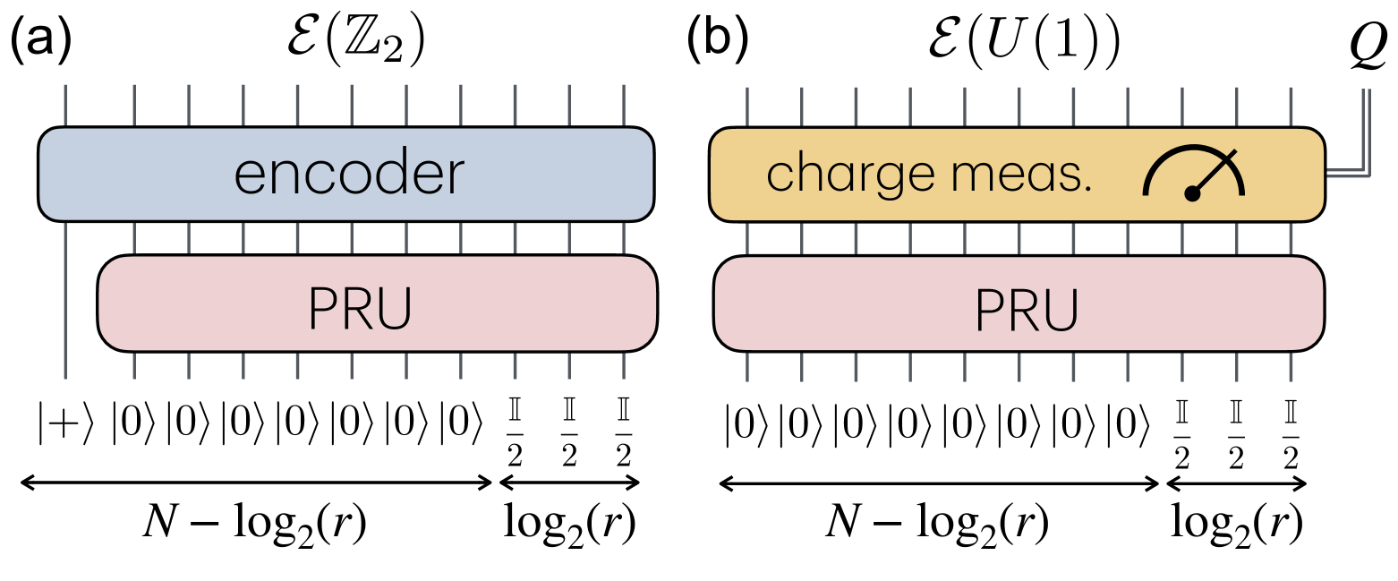
Figure 1: Circuits for the preparation of pseudo-SWSSB states with (a) $\mathbb{Z}_{2}$ symmetry or (b) $U(1)$ symmetry. In (a), the encoder is a staircase circuit of CNOT gates mapping $X_{1}$ to the symmetry generator $\bar{X}=\prod_{i}X_{i}$. In (b), the charge measurement can be implemented with $O(N)$ ancilla qubits and $O(\log(N))$ depth; postselection of an outcome $Q$ is sample-efficient as long as $Q=N/2+O(N^{1/2})$. To achieve pseudo-SWSSB the number of depolarized qubits $\log_{2}(r)$ must be superlogarithmic but subextensive.

Next we prove that $\mathcal{E}(\mathbb{Z}_{2})$ defined in Eq. (2) has pseudo-SWSSB if $r$ scales suitably with $N$. Note that, since every $\rho\in\mathcal{E}(\mathbb{Z}_{2})$ is proportional to a projector, we have $R_{1}(i,j)=R_{2}(i,j)$ and $R_{1}(i,j)\leq F(i,j)\leq\sqrt{R_{1}(i,j)}$ Liu et al. (2024); Weinstein (2024), so all three diagnostics have the same asymptotic behavior in this case. We thus focus only on $R_{1}(i,j)$ in the following unless specified.

Theorem 1 (Pseudo-SWSSB for $\mathbb{Z}_{2}$ symmetry).

For $r$ satisfying $\omega(\log N)<\log r<o(N)$, the ensemble $\mathcal{E}(\mathbb{Z}_{2})$ in Eq. (2) has pseudo-SWSSB.

Proof.

We prove the four conditions in Definition 1. (i) The ensemble is efficiently preparable as both the PRU and the encoder circuit have polynomial depth. (ii) Strong symmetry is ensured by the fact that each $\rho\in\mathcal{E}(\mathbb{Z}_{2})$ is supported inside the $\mathcal{H}_{+}$ symmetry sector: $\bar{X}\rho=+\rho$. (iii) The strong symmetry is unbroken because the Rényi-1 correlator $R_{1}(i,j)$ is negligibly small with high probability. This holds because each state $\rho$ in the ensemble is proportional to a rank-$r$ projector, so $\sqrt{\rho}=\sqrt{r}\rho$, and $R_{1}(i,j)=r{\rm Tr}(\rho O_{i}O_{j}^{\dagger}\rho O_{i}^{\dagger}O_{j})$. This is quadratic in $\rho=U\Pi_{r}U^{\dagger}/r$, and thus in the PRU $U$. Since the PFC ensemble contains a random Clifford unitary, it forms an exact 2-design. Thus the average of $R_{1}$ over the ensemble can be computed exactly; a straightforward calculation gives $\mathbb{E}_{\rho\sim\mathcal{E}(\mathbb{Z}_{2})}R_{1}(i,j)\leq O(r/d)$. Since $R_{1}(i,j)$ is non-negative (as seen by expanding $\rho$ in its eigenbasis), Markov’s inequality gives

$$\textsf{Pr}(R_{1}(i,j)>\delta)<O\left(\frac{r}{\delta d}\right)$$ (3)

for all $\delta>0$. Taking e.g. $\delta=d^{-1/2}$ shows that, if $r$ is sub-exponential, then $R_{1}(i,j)$ is exponentially small with probability exponentially close to 1. Thus that the strong symmetry is unbroken. (iv) Computational indistinguishability between $\rho_{0}$ and $\mathcal{E}(\mathbb{Z}_{2})$ can be proven in two steps. First we replace the PRUs by genuine Haar-random unitaries, defining the ensemble $\mathcal{E}^{\prime}(\mathbb{Z}_{2}):=\left\{{U\Pi_{r}U^{\dagger}}/{r}:\ U\sim\mathcal{U}_{\rm Haar}(\mathcal{H}_{+})\right\}$; this is computationally indistinguishable from $\mathcal{E}(\mathbb{Z}_{2})$ by the definition of PRUs. Then we prove the following (see Supplementary Information):

Lemma 1.

For $e^{\omega(\log N)}<r<e^{o(N)}$ and any number of state copies $k={\rm poly}(N)$, the ensemble $\mathcal{E}^{\prime}(\mathbb{Z}_{2})$ satisfies

$$\left\|{\mathbb{E}}_{\rho\sim\mathcal{E}^{\prime}(\mathbb{Z}_{2})}\rho^{\otimes k}-\rho_{0}^{\otimes k}\right\|_{\rm tr}\leq O\left(\frac{k^{2}}{r}\right).$$ (4)

This asserts the statistical indistinguishability  between the random ensemble $\mathcal{E}^{\prime}(\mathbb{Z}_{2})$ and $\rho_{0}$ for any number $k={\rm poly}(N)$ of copies. Thus $\mathcal{E}(\mathbb{Z}_{2})$ is indistinguishable from $\mathcal{E}^{\prime}(\mathbb{Z}_{2})$ which is indistinguishable from $\rho_{0}$, giving property (iv) and concluding the proof. ∎

Theorem 1 is one of the main results of this work. It proves the existence of efficiently preparable state ensembles that do not exhibit SWSSB but cannot be efficiently distinguished from the prototypical SWSSB state $\rho_{0}=(\mathbb{I}+\bar{X})/d$. Thus mixed-state phases of matter based on $\mathbb{Z}_{2}$ SWSSB can be hard to detect without additional structure or prior information on the system. How hard exactly? The largest error term in our analysis, Eq. (4), is $O(k^{2}/r)$. Thus, given a constant number $k$ of copies at a time (the most experimentally realistic scenario), it would take $\Omega(r^{2})$ experimental repetitions  to detect a discrepancy between $\mathcal{E}(\mathbb{Z}_{2})$ and $\rho_{0}$ with high confidence. This bound is saturated by measuring the purity ${\rm Tr}(\rho^{2})=1/r$ from two-copy measurements via SWAP test. It follows that no protocol using constant quantum memory is asymptotically more efficient than a brute-force measurement of $R_{2}$. While $R_{2}$ itself is not a reliable measure of SWSSB, recent work Zhang et al. (2024) finds a series expansion of the fidelity correlator $F$ in terms of higher-Rényi correlators $R_{2n}$, suggesting that a sample complexity of ${\rm poly}(r)$ should be sufficient to estimate $F$, in agreement with our result.

$U(1)$ symmetry.—We now generalize our finding from the discrete symmetry $\mathbb{Z}_{2}$ to the continuous symmetry $U(1)$. The latter acts on the Hilbert space as $e^{i\theta\sum_{i}(\mathbb{I}-Z_{i})/2}$ for $e^{i\theta}\in U(1)$, splitting the $N$-qubit Hilbert space into a direct sum of charge sector subspaces $\mathcal{H}_{Q}$ of dimension $d_{Q}=\binom{N}{Q}$, each spanned by computational basis states of Hamming weight $Q$. The standard choice for local charged operators is $O_{i}=S_{i}^{+}=(X_{i}+iY_{i})/2$ and $O_{i}^{\dagger}=S_{i}^{-}$. These are not unitary, so the fidelity correlator $F$ is ill-defined; we will focus on $R_{1}$ (one could alternatively take, e.g., $O_{i}=X_{i}$ without affecting our results). In analogy with the $\mathbb{Z}_{2}$ case, the reference state for $U(1)$ SWSSB is a maximally mixed state inside a charge sector subspace $\mathcal{H}_{Q}$, $\rho_{Q}=P_{Q}/d_{Q}$, with $P_{Q}$ the projector on $\mathcal{H}_{Q}$. $\rho_{Q}$ exhibits SWSSB if the charge density $\sigma:=\lim_{N\to\infty}Q/N$ is a finite constant not equal to 0 or 1 (see Supplementary Information).

Adapting the ensemble construction in Eq. (2) to the case of $U(1)$ symmetry is not straightforward because existing PRU ensembles require a Hilbert space with a qubit tensor product structure, while the charge sector we are interested in has dimension $\binom{N}{Q}$ which is not a power of 2 (or any one prime number). To avoid this issue, we follow a slightly different route sketched in Fig. 1(b). First we prepare a rank-$r$ mixed state $\Pi_{r}/r$ by depolarizing $\log_{2}(r)$ qubits in a pure product state; then we apply a PRU $U$ from the PFC ensemble to the whole $N$-qubit Hilbert space, obtaining a state $U\Pi_{r}U^{\dagger}/r$. At this point we perform a measurement of the charge $\frac{1}{2}\sum_{i}(Z_{i}-\mathbb{I})$, i.e., a Hamming weight projection, which can be done efficiently using $O(N)$ auxiliary qubits and $O(\log N)$ depth Rethinasamy et al. (2024). This measurement returns a value $Q$ of the charge distributed according to $p(Q)=d_{Q}/d=2^{-N}\binom{N}{Q}$, a binomial distribution with mean $N/2$ and standard deviation $\sqrt{N}/2$. Thus, each value of $Q$ in the range $N/2+O(\sqrt{N})$ is produced in the experiment with probability $\Omega(1/\sqrt{N})$, and can be postselected with polynomial sampling overhead. This protocol can be used to efficiently prepare the following ensemble for any value of $Q=N/2+O(\sqrt{N})$:

$$\mathcal{E}(U(1)):=\left\{\frac{P_{Q}U\Pi_{r}U^{\dagger}P_{Q}}{\Tr\left(P_{Q}U\Pi_{r}U^{\dagger}\right)}:\ U\sim\mathcal{U}_{\rm PRU}(\mathcal{H})\right\}.$$ (5)

The second main result of our work is that the above ensemble exhibits $U(1)$-SWSSB:

Theorem 2 (Pseudo-SWSSB for $U(1)$ symmetry).

$\mathcal{E}(U(1))$ in Eq. (5) has pseudo-SWSSB if $e^{\omega(\log N)}<r<e^{o(N)}$ and $|Q-N/2|\leq O(N^{1/2})$.

The proof is given in the Supplementary Information. Here we provide a brief sketch. Properties (i) and (ii) (efficient preparation and strong symmetry) are apparent from the construction described above. Property (iv) (computational indistinguishability) is proven similarly to the $\mathbb{Z}_{2}$ case (Lemma 1), with some additional complications in the Weingarten calculus due to the presence of $U$ in the denominator in Eq. (5). Finally to establish property (iii) (absence of SWSSB) we use the fact that the PFC PRUs form an exact 2-design to show that $\rho\in\mathcal{E}(U(1))$ is extremely close to a (trace-normalized) projector with high probability, and thus reduce $R_{1}(i,j)$ to a quadratic function of the PRU $U$ with negligible error. At that point the methods used in the $\mathbb{Z}_{2}$ case carry over.

Theorem 2 shows that our statements on the hardness of observing SWSSB apply not just to discrete symmetries, but also to continuous ones. This is a nontrivial generalization due to the richer structure of symmetry sector subspaces and their lack of tensor product structure. Our approach, based on charge measurements and (sample-efficient) postselection, is straightforwardly generalizable to other Abelian symmetry groups, such as products of multiple $U(1)$ and $\mathbb{Z}_{2}$ groups.

Discussion and outlook.—We have shown that the phenomenon of strong-to-weak symmetry breaking, a signature of intrinsically mixed phases of matter, can be hard to detect experimentally. In particular we have proven that, given only standard experimental access to copies of an unknown mixed state, no efficient experiment can in general decide whether or not the state has SWSSB. Our approach leverages recent ideas from quantum information and quantum cryptography Ji et al. (2018); Metger et al. (2024) to construct pseudorandom density matrices Bansal et al. (2025) that can hide their lack of SWSSB from any efficient experiment. While we rule out efficient state-agnostic protocols, efficient detection may still be possible in the presence of additional structure or prior information on the system Weinstein (2024).

Our work leaves several open questions. First, our construction only addresses on-site Abelian symmetries. Generalization to more complex symmetries such as non-Abelian or higher-form symmetries is an interesting future direction. A limitation of our approach for $U(1)$ symmetry is that we cannot efficiently prepare states away from the largest symmetry sector subspaces, i.e., at asymptotic charge density $\sigma=\lim_{N\to\infty}Q/N\neq 1/2$. This is due to our measurement-based approach to project PRUs on the whole Hilbert space into a fixed symmetry sector. To relax this limitation, it would be interesting to develop PRU ensembles that can target subspaces of arbitrary dimension.

By establishing a fundamental limitation on the observability of intrinsically mixed phases of matter, our work adds to a growing body of research that leverages pseudorandomness to understand the hardness of observing key properties of quantum many-body systems such as entanglement Aaronson et al. (2024); Giurgica-Tiron and Bouland (2023); Jeronimo et al. (2024); Cheng et al. (2024), thermalization Feng and Ippoliti (2025); Lee et al. (2024a), chaos Gu et al. (2024b); Lee et al. (2024b), nonstabilizerness Gu et al. (2024c), topological order Schuster et al. (2025), and holography Cheng et al. (2024); Engelhardt et al. (2024); Akers et al. (2024). A better understanding of which features are or are not efficiently observable in quantum experiments remains an essential goal for future research.

Acknowledgments. We thank Yuan Xue for helpful discussions. XF thanks Zhen Bi, Leonardo A. Lessa and Shengqi Sang for the useful discussions. XF was supported by a TQI Postdoctoral Fellowship.

Supplementary Information: Hardness of observing strong-to-weak symmetry breaking

S1 Review of useful facts about Weingarten calculus

Here we review some facts about Weingarten calculus which are used in our proofs.

Fact S1.1 ($k$-fold twirling channel).

We have

$$\Phi^{(k)}_{\rm Haar}(O)=\mathbb{E}_{U\sim{\rm Haar}}\left[U^{\otimes k}OU^{\dagger\otimes k}\right]=\sum_{\sigma,\tau\in S_{k}}\mathsf{Wg}_{d}(\sigma\tau^{-1})\Tr\left(\hat{\tau}^{-1}O\right)\hat{\sigma},$$ (S1)

where $\hat{\sigma}$ represents the action of permutation $\sigma\in S_{k}$ on the $k$ copies of the Hilbert space and $\textsf{Wg}_{d}$ is the Weingarten function on a $d$-dimensional Hilbert space. For $k=2$, we have

$$\mathsf{Wg}_{d}(e)=\frac{1}{d^{2}-1},\qquad\mathsf{Wg}_{d}(\pi)=-\frac{1}{d(d^{2}-1)},$$ (S2)

where $e,\pi\in S_{2}$ are the identity and the transposition respectively.

Fact S1.2 (Bounds for absolute value of Weigarten function Collins and Matsumoto (2017); Cheng et al. (2024)).

We have

$$|\mathsf{Wg}_{d}(\sigma)|\leq d^{-k}\left(\frac{d}{4}\right)^{|\sigma|-k}\left[1+O\left(\frac{k^{7/2}}{d^{2}}\right)\right]$$ (S3)

where $|\sigma|$ is the number of cylces in permutation $\sigma$. Additionally, for $\sigma=e$ (identity permutation), we have Zhou and Nahum (2019)

$$\mathsf{Wg}_{d}(e)=d^{-k}\left[1+O\left(\frac{k^{2}}{d^{2}}\right)\right].$$ (S4)

Fact S1.3 (Gram matrix sum).

We have

$$\sum_{\sigma\in S_{k}}d^{|\sigma|}=\frac{(d-1+k)!}{(d-1)!}=d^{k}\left[1+O\left(\frac{k^{2}}{d}\right)\right].$$ (S5)

S2 Proof of Lemma 1

Here we will prove the statistical indistinguishability between the random ensemble $\mathcal{E}^{\prime}(\mathbb{Z}_{2})$ and the state $\rho_{0}=(\mathbb{I}+\bar{X})/d=(2/d)P_{0}$. We take a number of state copies $k={\rm poly}(N)$ and focus on the regime $e^{\omega(\log N)}<r<e^{o(N)}$ for the parameter $r$ that sets the rank of states in the ensemble.

We first use Fact S1.1 to rewrite $\mathbb{E}_{\rho\sim\mathcal{E}^{\prime}(\mathbb{Z}_{2})}\rho^{\otimes k}=\Phi^{(k)}_{\rm Haar}(\Pi_{r}^{\otimes k}/r^{k})=\sum_{\sigma,\tau\in S_{k}}\textsf{Wg}_{d/2}(\sigma\tau^{-1})\frac{r^{|\tau|}}{r^{k}}\hat{\sigma}$. Recall that the Haar measure is over the subspace $\bar{X}=+1$, of dimension $d/2$. Then, the trace distance can be bounded as

$$\left\|\sum_{\sigma,\tau\in S_{k}}\textsf{Wg}_{d/2}(\sigma\tau^{-1})\frac{r^{|\tau|}}{r^{k}}\hat{\sigma}-\frac{P_{0}^{\otimes k}}{(d/2)^{k}}\right\|_{\rm tr}\leq\left|\sum_{\tau\in S_{k}}\textsf{Wg}_{d/2}(\tau^{-1})\frac{r^{|\tau|}}{r^{k}}\left(\frac{d}{2}\right)^{k}-1\right|+\left\|\sum_{\begin{subarray}{c}\sigma,\tau\in S_{k}:\\ \sigma\neq e\end{subarray}}\textsf{Wg}_{d/2}(\sigma\tau^{-1})\frac{r^{|\tau|}}{r^{k}}\hat{\sigma}\right\|_{\rm tr},$$ (S6)

where we used the fact that $\hat{e}=P_{0}^{\otimes k}$ and $\|P_{0}\|_{\rm tr}=d/2$.

The first term of the right hand side of Eq.(S6) can be further bounded by the sum of $\textsf{Wg}_{d/2}(e)=(2/d)^{k}[1+O(k^{2}/d^{2})]$ (Fact S1.2) and

$$\left|\sum_{\tau\in S_{k}:\ \tau\neq e}\textsf{Wg}_{d/2}\left(\tau^{-1}\right)\frac{r^{|\tau|}(d/2)^{k}}{r^{k}}\right|\leq -1+\sum_{\tau\in S_{k}}\left|\textsf{Wg}_{d/2}\left(\tau^{-1}\right)\right|\frac{r^{|\tau|}(d/2)^{k}}{r^{k}}$$

$$\leq -1+\sum_{\tau\in S_{k}}\left(\frac{dr}{8}\right)^{|\tau|-k}\left[1+O\left(\frac{k^{7/2}}{d^{2}}\right)\right]=O\left(\frac{k^{2}}{rd}\right),$$ (S7)

where we used Facts S1.2 and S1.3. For the second term on the right hand side of Eq.(S6), we can use the inequaility $\left\|A\right\|_{\rm tr}\leq\textsf{dim}\cdot\left\|A\right\|_{\rm op}$ with dim the Hilbert space dimension, and Facts S1.2 and S1.3, to get

$$\left\|\sum_{\begin{subarray}{c}\sigma,\tau\in S_{k}:\\ \sigma\neq e\end{subarray}}\textsf{Wg}_{d/2}\left(\sigma\tau^{-1}\right)\frac{r^{|\tau|}}{r^{k}}\hat{\sigma}\right\|_{\rm tr}\leq \left\|\sum_{\begin{subarray}{c}\sigma,\tau\in S_{k}:\\ \sigma\neq e\end{subarray}}\textsf{Wg}_{d/2}\left(\sigma\tau^{-1}\right)\frac{r^{|\tau|}\left(d/2\right)^{k}}{r^{k}}\hat{\sigma}\right\|_{\rm op}$$

$$\leq -1+\sum_{\sigma,\tau\in S_{k}}\left|\textsf{Wg}_{d/2}\left(\sigma\tau^{-1}\right)\right|\frac{r^{|\tau|}(d/2)^{k}}{r^{k}}$$

$$\leq -1+\sum_{\sigma,\tau\in S_{k}}\left(\frac{d}{8}\right)^{\left|\sigma\tau^{-1}\right|-k}r^{|\tau|-k}\left[1+O\left(\frac{k^{7/2}}{d^{2}}\right)\right]=O\left(\frac{k^{2}}{r}\right).$$ (S8)

Plugging the two bounds back in Eq. (S6), we obtain the statement of Lemma 1:

$$\left\|\mathbb{E}_{\rho\sim\mathcal{E}^{\prime}(\mathbb{Z}_{2})}\rho^{\otimes k}-\rho^{\otimes k}\right\|_{\rm tr}\leq O\left(\frac{k^{2}}{r}\right).$$ (S9)

S3 Proof of Theorem 2

Here we prove Theorem 2, asserting pseudo-SWSSB in the ensemble $\mathcal{E}(U(1))$ of Eq. (5). Let us briefly summarize some notation. The $U(1)$ symmetry action is $U_{g}(\theta)=e^{i\theta\hat{Q}}$ with charge operator $\hat{Q}=\sum_{i}(\mathbb{I}-Z_{i})/2$. The Hilbert space is the direct sum of symmetry sectors, $\mathcal{H}=\bigoplus_{Q=0}^{N}\mathcal{H}_{Q}$. Each $\mathcal{H}_{Q}$ is spanned by computational basis states of Hamming weight $Q$ and has dimension $d_{Q}=\binom{N}{Q}$. To diagnose SWSSB we choose local charged operators $O_{i}=S_{i}^{+}=(X_{i}+iY_{i})/2$. These are not unitary, so the fidelity correlator $F$ is not defined; we use $R_{1}$ instead.

First, we show that the states $\rho_{Q}=P_{Q}/d_{Q}$ (maximally mixed states in a charge sector) exhibit SWSSB when the charge density $\sigma=Q/N$ is asymptotically not 0 or 1. Clearly $\rho_{Q}$ has a strong symmetry: $U_{g}(\theta)\rho_{Q}=e^{i\theta Q}\rho_{Q}$. Also, the ordinary correlator $C(i,j)=\Tr(S_{i}^{+}S_{j}^{-}P_{Q}/d_{Q})=0$ vanishes by the definition of $P_{Q}$ (as seen e.g. by taking the trace in the computational basis), so the weak symmetry is unbroken. However, the the Rényi-1 correlator is given by

$$R_{1}(i,j)=\frac{1}{d_{Q}}\Tr(P_{Q}S_{i}^{+}S_{j}^{-}P_{Q}S_{j}^{+}S_{i}^{-})=\frac{1}{d_{Q}}\binom{N-2}{Q-1}=\frac{Q(N-Q)}{N(N-1)}=\sigma(1-\sigma)+o(1),$$ (S10)

where $\binom{N-2}{Q-1}$ is the number of computational basis states with total Hamming weight $Q$, a $|0\rangle$ at site $i$, and a $|1\rangle$ at site $j$. This is a finite constant as long as $\sigma\neq 0,1$, showing spontaneous breaking of the strong symmetry.

Next, we show that the pseudorandom state ensemble

$$\mathcal{E}(U(1))=\left\{\frac{P_{Q}U\Pi_{r}U^{\dagger}P_{Q}}{\Tr\left(P_{Q}U\Pi_{r}U^{\dagger}P_{Q}\right)}:\ U\sim\mathcal{U}_{\rm PRU}(\mathcal{H})\right\}$$ (S11)

does not break the strong symmetry; see Lemma 2.

Finally, to show computational indistinguishability of $\mathcal{E}(U(1))$ from $\rho_{Q}$, we first use the definition of PRUs to replace $\mathcal{E}(U(1))$ by its Haar-random counterpart

$$\mathcal{E}^{\prime}(U(1))=\left\{\frac{P_{Q}U\Pi_{r}U^{\dagger}P_{Q}}{\Tr\left(P_{Q}U\Pi_{r}U^{\dagger}P_{Q}\right)}:\ U\sim\mathcal{U}_{\rm Haar}(\mathcal{H})\right\}$$ (S12)

in a computationally undetectable way; then we show that $\mathcal{E}^{\prime}(U(1))$ is statistically indistinguishable from $\rho_{Q}$, see Lemma 3. This concludes the proof of pseudo-SWSSB in $\mathcal{E}(U(1))$.

Lemma 2 (absence of SWSSB in $\mathcal{E}(U(1))$).

The Rényi-1 correlator is superpolynomially small with high probability over the pseudorandom ensemble $\mathcal{E}(U(1))$: for all $\delta>0$, we have

$${\sf Prob}\left(|R_{1}(i,j)|\geq\delta\right)\leq O\left(\frac{r^{3/2}}{\delta d_{Q}^{1/4}}\right).$$ (S13)

Proof.

We will first show that the states $\rho\in\mathcal{E}(U(1))$ are extremely close to rank-$r$ projectors (up to the trace normalization) with high probability; that will let us reduce the expression for $R_{1}$ to a quadratic polynomial in $U,U^{\dagger}$, where we can use the 2-design propertyAmbainis and Emerson (2007); Dankert et al. (2009); Roberts and Yoshida (2017) to switch from the pseudorandom ensemble $\mathcal{U}_{\rm PRU}$ to the Haar-random ensemble and conclude the proof.

Let us first define the operators $\tilde{\rho}=\frac{d}{d_{Q}r}P_{Q}U\Pi_{r}U^{\dagger}P_{Q}$. These are un-normalized “states” of rank $\leq r$ ($\Pi_{r}$ has rank $r$ by definition, and conjugation by $P_{Q}$ cannot increase the rank). It is straightforward to show, using the 2-design property of $\mathcal{U}_{\rm PRU}$ and Weingarten calculus, that

$$\mathbb{E}_{U\sim\mathcal{U}_{\rm PRU}}{\rm Tr}(\tilde{\rho})=1,\quad\mathbb{E}_{U\sim\mathcal{U}_{\rm PRU}}{\rm Tr}(\tilde{\rho}^{2})=\frac{1}{r}+O\left(\frac{1}{d_{Q}}\right).$$ (S14)

Thus the $\tilde{\rho}$ “states” are normalized on average and nearly maximally mixed on their rank-$r$ support. Specifically, let us write the (nonzero) eigenvalues of $\tilde{\rho}$ as $\{1/r+\delta_{i}\}_{i=1}^{r}$; pluggint these into Eq. (S14) we see that the $\delta_{i}$ satisfy

$$\sum_{i}\mathbb{E}_{U\sim\mathcal{U}_{\rm PRU}}[\delta_{i}]=0,\quad\sum_{i}\mathbb{E}_{U\sim\mathcal{U}_{\rm PRU}}[\delta_{i}^{2}]=O(1/d_{Q}).$$ (S15)

By Markov’s inequality, we have $\textsf{Pr}\left((\sum_{i}\delta_{i}^{2})>c\right)\leq O(1/(cd_{Q}))$, and choosing e.g. $c=1/d_{Q}^{1/2}$ we have that $\sum_{i}\delta_{i}^{2}\leq O\left(1/d_{Q}^{1/2}\right)$ with probability at least $1-O\left(1/d_{Q}^{1/2}\right)$.

As a consequence, when $\sum_{i}\delta_{i}^{2}\leq O(1/d_{Q}^{1/2})$, $\sqrt{\rho}$ is extremely close to $\sqrt{r}\tilde{\rho}$: recalling that $\rho=\tilde{\rho}/{\rm Tr}(\tilde{\rho})$, we have

$$\left\|\sqrt{\rho}-\sqrt{r}\tilde{\rho}\right\|_{\rm tr} =\sum_{i=1}^{r}\left|\left({\frac{1+r\delta_{i}}{\sum_{j=1}^{r}(1+r\delta_{j})}}\right)^{1/2}-\frac{1+r\delta_{i}}{\sqrt{r}}\right|$$

$$\leq\sum_{i=1}^{r}\frac{1}{\sqrt{r}}\left(\left|\left({\frac{1+r\delta_{i}}{1+\sum_{j=1}^{r}\delta_{j}}}\right)^{1/2}-1\right|+r|\delta_{i}|\right)$$

$$\leq 2\sqrt{r}\sum_{i=1}^{r}|\delta_{i}|\leq 2r\left(\sum_{i}\delta_{i}^{2}\right)^{1/2}\leq O\left(\frac{r}{d_{Q}^{1/4}}\right).$$ (S16)

where we have used $\sum_{i}\delta_{i}\leq\sum_{i}|\delta_{i}|\leq\sqrt{r\sum_{i}\delta_{i}^{2}}$ (by Cauchy-Schwarz). Thus the Rényi-1 correlator simplifies: letting $B=O_{i}O_{j}^{\dagger}$, we have

$$R_{1}(i,j) ={\rm Tr}(\sqrt{\rho}B\sqrt{\rho}B^{\dagger})$$

$$=\sqrt{r}{\rm Tr}(\tilde{\rho}B\sqrt{\rho}B)+{\rm Tr}((\sqrt{\rho}-\sqrt{r}\tilde{\rho})B\sqrt{\rho}B^{\dagger})$$

$$\leq\sqrt{r}{\rm Tr}(\tilde{\rho}B\sqrt{\rho}B)+\|\sqrt{\rho}-\sqrt{r}\tilde{\rho}\|_{\rm tr}\|B\sqrt{\rho}B^{\dagger}\|_{\rm op}$$

$$\leq\sqrt{r}{\rm Tr}(\tilde{\rho}B\sqrt{\rho}B)+O\left(r/d_{Q}^{1/4}\right),$$ (S17)

where we used the inequality $\|AB\|_{\rm tr}\leq\|A\|_{\rm tr}\|B\|_{\rm op}$, the bound from Eq. (S16), and the fact that $\|B\sqrt{\rho}B^{\dagger}\|_{\rm op}\leq\|B\|_{\rm op}^{2}\|\rho\|_{\rm op}^{1/2}\leq 1$. Iterating the same argument on the remaining $\sqrt{\rho}$ operator, one gets

$$R_{1}(i,j) \leq r{\rm Tr}(\tilde{\rho}B\tilde{\rho}B^{\dagger})+\sqrt{r}\|\sqrt{\rho}-\sqrt{r}\tilde{\rho}\|_{\rm tr}\|B\rho B^{\dagger}\|_{\rm op}{\rm Tr}(\tilde{\rho})+O\left(r/d_{Q}^{1/4}\right)$$

$$\leq r{\rm Tr}(\tilde{\rho}B\tilde{\rho}B^{\dagger})+{\rm Tr}(\tilde{\rho})O\left(r^{3/2}/d_{Q}^{1/4}\right),$$ (S18)

where we also used $\tilde{\rho}=\rho{\rm Tr}(\tilde{\rho})$. Finally we can average over ${U\sim\mathcal{U}_{\rm PRU}}$, breaking down the average between elements where $\sum_{i}\delta_{i}^{2}<c/d_{Q}^{1/2}$ and the rest. Calling the first event $\mathcal{A}$ and its complement $\bar{\mathcal{A}}$, we have

$$\mathbb{E}_{U\sim\mathcal{U}_{\rm PRU}}R_{1}(i,j) =\textsf{Pr}(\mathcal{A})\mathbb{E}_{U\sim\mathcal{U}_{PRU}|\mathcal{A}}\left[R_{1}(i,j)\right]+\textsf{Pr}(\bar{\mathcal{A}})\mathbb{E}_{U\sim\mathcal{U}_{PRU}|\bar{\mathcal{A}}}\left[R_{1}(i,j)\right]$$

$$\leq r\mathbb{E}_{U\sim\mathcal{U}_{\rm PRU}}[{\rm Tr}(\tilde{\rho}O_{i}O_{j}^{\dagger}\tilde{\rho}O_{i}^{\dagger}O_{j})]+O\left(\frac{r^{3/2}}{d_{Q}^{1/4}}\right)+P(\bar{\mathcal{A}})$$

$$\leq\mathbb{E}_{U\sim\mathcal{U}_{\rm PRU}}[{\rm Tr}(\tilde{\rho}O_{i}O_{j}^{\dagger}\tilde{\rho}O_{i}^{\dagger}O_{j})]+O\left(\frac{r^{3/2}}{d_{Q}^{1/4}}\right)+O\left(\frac{1}{d_{Q}^{1/2}}\right),$$ (S19)

Here we have used the facts that $\textsf{Pr}(\mathcal{A})\mathbb{E}_{|\mathcal{A}}[R_{1}]\leq\mathbb{E}[R_{1}]$ since $R_{1}$ is always non-negative and $R_{1}\leq 1$, along with the fact that $\textsf{Pr}(\bar{\mathcal{A}})\leq O(1/d_{Q}^{1/2})$. At this point, since the quantity to average is quadratic in $U$ and $\mathcal{U}_{\rm PRU}$ forms an exact 2-design, we may replace the PRU ensemble by the Haar ensemble:

$$\mathbb{E}_{U\sim\mathcal{U}_{\rm PRU}}R_{1}(i,j) \leq r\frac{d^{2}}{d_{Q}^{2}}\mathbb{E}_{U\sim\mathcal{U}_{\rm Haar}}\left[{\rm Tr}\left(P_{Q}U\frac{\Pi_{r}}{r}U^{\dagger}P_{Q}O_{i}O_{j}^{\dagger}P_{Q}U\frac{\Pi_{r}}{r}U^{\dagger}P_{Q}O_{i}^{\dagger}O_{j}\right)\right]+O\left(\frac{r^{3/2}}{d_{Q}^{1/4}}\right)$$

$$\leq r\frac{d^{2}}{d_{Q}^{2}}{\rm Tr}\left[\Phi^{(2)}_{\rm Haar}\left(\frac{\Pi_{r}^{\otimes 2}}{r^{2}}\right)(P_{Q}O_{i}O_{j}^{\dagger}P_{Q})\otimes(P_{Q}O_{i}^{\dagger}O_{j}P_{Q})\hat{\pi}\right]+O\left(\frac{r^{3/2}}{d_{Q}^{1/4}}\right)$$

$$\leq\frac{r}{d_{Q}^{2}}\frac{d^{2}}{d^{2}-1}\left(1-\frac{1}{rd}\right){\rm Tr}(P_{Q}O_{i}^{\dagger}O_{j}P_{Q}O_{i}O_{j}^{\dagger})+O\left(\frac{r^{3/2}}{d_{Q}^{1/4}}\right)$$

$$\leq\frac{r}{d_{Q}}+O\left(\frac{r^{3/2}}{d_{Q}^{1/4}}\right)\leq O\left(\frac{r^{3/2}}{d_{Q}^{1/4}}\right).$$ (S20)

Here we used Fact S1.1 to expand the Haar twirling channel. We then used the fact that ${\rm Tr}(P_{Q}O_{i}O_{j}^{\dagger})=0$ and that ${\rm Tr}(P_{Q}O_{i}O_{j}^{\dagger}P_{Q}O_{i}^{\dagger}O_{j})\leq d_{Q}$, as seen e.g. by taking the trace in the computational basis. Finally, Markov’s inequality yields the result. ∎

Lemma 3 (Statistical indistinguishability between $\rho_{Q}$ and $\mathcal{E}^{\prime}(U(1))$).

$$\left\|\mathbb{E}_{\rho\sim\mathcal{E}^{\prime}(U(1))}\rho^{\otimes k}-\rho_{Q}^{\otimes k}\right\|_{\rm tr}\leq O\left(\frac{k^{2}}{r}\right).$$ (S21)

Proof.

We again introduce the unnormalized density matrix $\tilde{\rho}:=\frac{d}{rd_{Q}}P_{Q}U\Pi_{r}U^{\dagger}P_{Q}$ and recall that $\rho_{Q}=P_{Q}/d_{Q}$. Since $\rho=\tilde{\rho}/{\rm Tr}(\tilde{\rho})$, by the triangle inequality we have

$$\left\|\mathbb{E}_{U}\frac{\tilde{\rho}^{\otimes k}}{\left(\Tr\tilde{\rho}\right)^{k}}-\frac{P_{Q}^{\otimes k}}{d_{Q}^{k}}\right\|_{\rm tr}\leq \left\|\mathbb{E}_{U}\frac{\tilde{\rho}^{\otimes k}}{\left(\Tr\tilde{\rho}\right)^{k}}-\frac{\mathbb{E}_{U}\tilde{\rho}^{\otimes k}}{\mathbb{E}_{U}\left(\Tr\tilde{\rho}\right)^{k}}\right\|_{\rm tr}+\left\|\frac{\mathbb{E}_{U}\tilde{\rho}^{\otimes k}}{\mathbb{E}_{U}\left(\Tr\tilde{\rho}\right)^{k}}-\frac{P_{Q}^{\otimes k}}{d_{Q}^{k}}\right\|_{\rm tr}.$$ (S22)

where $\mathbb{E}_{U}$ stands for $\mathbb{E}_{U\sim\mathcal{U}_{\rm Haar}}$ in the following.

For the first term in the right hand side of Eq. (S22), we have

$$\left\|\mathbb{E}_{U}\frac{\tilde{\rho}^{\otimes k}}{\left(\Tr\tilde{\rho}\right)^{k}}-\frac{\mathbb{E}_{U}\tilde{\rho}^{\otimes k}}{\mathbb{E}_{U}\left(\Tr\tilde{\rho}\right)^{k}}\right\|_{\rm tr} \leq\left\|\mathbb{E}_{U}\left[\rho^{\otimes k}\left(1-\frac{({\rm Tr}\tilde{\rho})^{k}}{\mathbb{E}_{U^{\prime}}({\rm Tr}\tilde{\rho})^{k}}\right)\right]\right\|_{\rm tr}$$

$$\leq\mathbb{E}_{U}\left|1-\frac{\left(\Tr\tilde{\rho}\right)^{k}}{\mathbb{E}_{U^{\prime}}\left(\Tr\tilde{\rho}\right)^{k}}\right|$$

$$\leq\sqrt{\frac{\mathbb{E}_{U}\left(\Tr\tilde{\rho}\right)^{2k}}{\left(\mathbb{E}_{U}\left(\Tr\tilde{\rho}\right)^{k}\right)^{2}}-1},$$ (S23)

where we have used Jensen’s inequality for the function $\sqrt{x}$. Now we define $f(k):=\mathbb{E}_{U}\left(\Tr\tilde{\rho}\right)^{k}$, so that the above bound is given by $\sqrt{f(2k)/f(k)^{2}-1}$. Using Fact S1.1, we have

$$f(k) =\left(\frac{d}{rd_{Q}}\right)^{k}\sum_{\sigma,\tau\in S_{k}}\mathsf{Wg}_{d}(\sigma\tau^{-1})r^{|\tau|}d_{Q}^{|\sigma|}$$

$$=1+O\left(\frac{k^{2}}{d^{2}}\right)+\sum_{\begin{subarray}{c}\sigma,\tau\in S_{k}:\\ (\sigma,\tau)\neq(e,e)\end{subarray}}d^{k}\mathsf{Wg}_{d}(\sigma\tau^{-1})r^{|\tau|-k}d_{Q}^{|\sigma|-k}.$$ (S24)

We then bound the summation over $(\sigma,\tau)\neq(e,e)$ by

$$\left|\sum_{\begin{subarray}{c}\sigma,\tau\in S_{k}:\\ (\sigma,\tau)\neq(e,e)\end{subarray}}d^{k}\mathsf{Wg}_{d}(\sigma\tau^{-1})r^{|\tau|-k}d_{Q}^{|\sigma|-k}\right| \leq\sum_{\sigma,\tau\in S_{k}}d^{k}\left|\mathsf{Wg}_{d}(\sigma\tau^{-1})\right|r^{|\tau|-k}d_{Q}^{|\sigma|-k}-1$$

$$\leq\sum_{\sigma,\tau\in S_{k}}\left(\frac{d}{4}\right)^{|\sigma\tau^{-1}|-k}r^{|\tau|-k}d_{Q}^{|\sigma|-k}\left[1+O\left(\frac{k^{7/2}}{d^{2}}\right)\right]-1$$

$$\leq\sum_{\sigma,\tau\in S_{k}}\left(\frac{d}{4}\right)^{|\sigma\tau^{-1}|-k}d_{Q}^{|\sigma|-k}\left[1+O\left(\frac{k^{7/2}}{d^{2}}\right)\right]-1$$

$$\leq O\left(\frac{k^{2}}{d_{Q}}\right),$$ (S25)

where we have used Facts S1.2 and S1.3. In all, we have $f(k)=1+O\left(\frac{k^{2}}{d_{Q}}\right)$ and thus

$$\sqrt{\frac{f(2k)}{f(k)^{2}}-1}=O\left(\frac{k^{2}}{d_{Q}}\right),$$ (S26)

which provides a negligible upper bound on the first term in Eq. (S22).

Moving on to the second term in Eq. (S22), we have

$$\left\|\frac{\mathbb{E}_{U}\tilde{\rho}^{\otimes k}}{\mathbb{E}_{U}\left(\Tr\tilde{\rho}\right)^{k}}-\frac{P_{Q}^{\otimes k}}{d_{Q}^{k}}\right\|_{\rm tr} =\left\|\frac{\sum_{\sigma,\tau\in S_{k}}d^{k}\mathsf{Wg}_{d}(\sigma\tau^{-1})r^{|\tau|-k}P_{Q}^{\otimes k}\hat{\sigma}P_{Q}^{\otimes k}}{d_{Q}^{k}f(k)}-\frac{P_{Q}^{\otimes k}}{d_{Q}^{k}}\right\|_{\rm tr}$$

$$\leq\left|\frac{\sum_{\tau\in S_{k}}d^{k}\mathsf{Wg}_{d}\left(\tau\right)r^{|\tau|-k}}{f(k)}-1\right|+\left\|\frac{\sum_{\sigma,\tau\in S_{k}:\ \sigma\neq e}d^{k}\mathsf{Wg}_{d}(\sigma\tau^{-1})r^{|\tau|-k}P_{Q}^{\otimes k}\hat{\sigma}P_{Q}^{\otimes k}}{d_{Q}^{k}f(k)}\right\|_{\rm tr},$$ (S27)

where we have separated the $\sigma=e$ term from the $\sigma\neq e$ terms. The former is bounded by

$$\left|\frac{\sum_{\tau\in S_{k}}d^{k}\mathsf{Wg}_{d}\left(\tau\right)r^{|\tau|-k}}{f(k)}-1\right| \leq\left|\frac{\sum_{\tau\neq e}d^{k}\mathsf{Wg}_{d}\left(\tau\right)r^{|\tau|-k}}{f(k)}\right|+\left|\frac{d^{k}\mathsf{Wg}_{d}\left(e\right)}{f(k)}-1\right|$$

$$\leq\frac{d^{k}\sum_{\tau\neq e}\left|\mathsf{Wg}_{d}\left(\tau\right)\right|r^{|\tau|-k}}{f(k)}+O\left(\frac{k^{2}}{d_{Q}}\right)$$

$$\leq\frac{1}{f(k)}\sum_{\tau\neq e}\left(\frac{rd}{4}\right)^{|\tau|-k}\left[1+O\left(\frac{k^{7/2}}{d^{2}}\right)\right]+O\left(\frac{k^{2}}{d_{Q}}\right)$$

$$\leq O\left(\frac{k^{2}}{d_{Q}}\right),$$ (S28)

where we have used Facts S1.2 and S1.3; the latter is bounded by

$$\left\|\frac{1}{d_{Q}^{k}f(k)}\sum_{\begin{subarray}{c}\sigma,\tau\in S_{k}:\\ \sigma\neq e\end{subarray}}d^{k}\mathsf{Wg}_{d}(\sigma\tau^{-1})r^{|\tau|-k}P_{Q}^{\otimes k}\hat{\sigma}P_{Q}^{\otimes k}\right\|_{\rm tr} \leq\frac{d^{k}}{d_{Q}^{k}f(k)}\sum_{\begin{subarray}{c}\sigma,\tau\in S_{k}:\\ \sigma\neq e\end{subarray}}\left|\mathsf{Wg}_{d}(\sigma\tau^{-1})\right|r^{|\tau|-k}\left\|P_{Q}^{\otimes k}\hat{\sigma}P_{Q}^{\otimes k}\right\|_{\rm tr}$$

$$\leq\frac{d^{k}}{d_{Q}^{k}f(k)}\sum_{\begin{subarray}{c}\sigma,\tau\in S_{k}:\\ \sigma\neq e\end{subarray}}\left|\mathsf{Wg}_{d}(\sigma\tau^{-1})\right|r^{|\tau|-k}\left\|P_{Q}^{\otimes k}\hat{\sigma}P_{Q}^{\otimes k}\right\|_{\rm op}d_{Q}^{k}$$

$$\leq\frac{d^{k}}{f(k)}\sum_{\begin{subarray}{c}\sigma,\tau\in S_{k}:\\ \sigma\neq e\end{subarray}}\left|\mathsf{Wg}_{d}(\sigma\tau^{-1})\right|r^{|\tau|-k}$$

$$\leq\frac{1}{f(k)}\left[\sum_{\begin{subarray}{c}\sigma,\tau\in S_{k}:\\ \sigma\neq e\end{subarray}}\left(\frac{d}{4}\right)^{|\sigma\tau^{-1}|-k}r^{|\tau|-k}\right]\left[1+O\left(\frac{k^{7/2}}{d^{2}}\right)\right]$$

$$\leq O\left(\frac{k^{2}}{r}\right),$$ (S29)

where we used Facts S1.2 and S1.3 and inequality $\|AB\|_{\rm tr}\leq\|A\|_{\rm op}\|B\|_{\rm tr}$. Combining all above contributions, we find that the leading error term is $O(k^{2}/r)$, thus completing the proof. ∎

References

- Wen (2017) Xiao-Gang Wen, “Colloquium: Zoo of quantum-topological phases of matter,” Rev. Mod. Phys. 89, 041004 (2017).
- Dennis et al. (2002) Eric Dennis, Alexei Kitaev, Andrew Landahl, and John Preskill, “Topological quantum memory,” Journal of Mathematical Physics 43, 4452–4505 (2002).
- Hastings (2011) Matthew B. Hastings, “Topological order at nonzero temperature,” Phys. Rev. Lett. 107, 210501 (2011).
- Lu et al. (2020) Tsung-Cheng Lu, Timothy H. Hsieh, and Tarun Grover, “Detecting topological order at finite temperature using entanglement negativity,” Phys. Rev. Lett. 125, 116801 (2020).
- Fan et al. (2024) Ruihua Fan, Yimu Bao, Ehud Altman, and Ashvin Vishwanath, “Diagnostics of mixed-state topological order and breakdown of quantum memory,” PRX Quantum 5, 020343 (2024).
- Lee et al. (2023) Jong Yeon Lee, Chao-Ming Jian, and Cenke Xu, “Quantum criticality under decoherence or weak measurement,” PRX Quantum 4, 030317 (2023).
- Lee et al. (2025) Jong Yeon Lee, Yi-Zhuang You, and Cenke Xu, “Symmetry protected topological phases under decoherence,” Quantum 9, 1607 (2025).
- Lessa et al. (2025) Leonardo A. Lessa, Ruochen Ma, Jian-Hao Zhang, Zhen Bi, Meng Cheng, and Chong Wang, “Strong-to-weak spontaneous symmetry breaking in mixed quantum states,” PRX Quantum 6, 010344 (2025).
- Wang et al. (2025) Zijian Wang, Zhengzhi Wu, and Zhong Wang, “Intrinsic mixed-state topological order,” PRX Quantum 6, 010314 (2025).
- Ellison and Cheng (2025) Tyler D. Ellison and Meng Cheng, “Toward a classification of mixed-state topological orders in two dimensions,” PRX Quantum 6, 010315 (2025).
- Sohal and Prem (2025) Ramanjit Sohal and Abhinav Prem, “Noisy approach to intrinsically mixed-state topological order,” PRX Quantum 6, 010313 (2025).
- Zhang et al. (2025) Carolyn Zhang, Yichen Xu, Jian-Hao Zhang, Cenke Xu, Zhen Bi, and Zhu-Xi Luo, “Strong-to-weak spontaneous breaking of 1-form symmetry and intrinsically mixed topological order,” Phys. Rev. B 111, 115137 (2025).
- Chen and Grover (2024) Yu-Hsueh Chen and Tarun Grover, “Separability transitions in topological states induced by local decoherence,” Phys. Rev. Lett. 132, 170602 (2024).
- Ma et al. (2025) Ruochen Ma, Jian-Hao Zhang, Zhen Bi, Meng Cheng, and Chong Wang, “Topological phases with average symmetries: the decohered, the disordered, and the intrinsic,” (2025), arXiv:2305.16399 [cond-mat.str-el] .
- Ma and Turzillo (2025) Ruochen Ma and Alex Turzillo, “Symmetry-protected topological phases of mixed states in the doubled space,” PRX Quantum 6, 010348 (2025).
- Kuno et al. (2024) Yoshihito Kuno, Takahiro Orito, and Ikuo Ichinose, “Strong-to-weak symmetry breaking states in stochastic dephasing stabilizer circuits,” Phys. Rev. B 110, 094106 (2024).
- Gu et al. (2024a) Ding Gu, Zijian Wang, and Zhong Wang, “Spontaneous symmetry breaking in open quantum systems: strong, weak, and strong-to-weak,” (2024a), arXiv:2406.19381 [quant-ph] .
- Zhang et al. (2024) Jian-Hao Zhang, Cenke Xu, and Yichen Xu, “Fluctuation-dissipation theorem and information geometry in open quantum systems,” (2024), arXiv:2409.18944 [quant-ph] .
- Huang et al. (2025) Xiaoyang Huang, Marvin Qi, Jian-Hao Zhang, and Andrew Lucas, “Hydrodynamics as the effective field theory of strong-to-weak spontaneous symmetry breaking,” Phys. Rev. B 111, 125147 (2025).
- Sachdev (2011) Subir Sachdev, Quantum Phase Transitions, 2nd ed. (Cambridge University Press, 2011).
- Sala et al. (2024) Pablo Sala, Sarang Gopalakrishnan, Masaki Oshikawa, and Yizhi You, “Spontaneous strong symmetry breaking in open systems: Purification perspective,” Phys. Rev. B 110, 155150 (2024).
- Weinstein (2024) Zack Weinstein, “Efficient detection of strong-to-weak spontaneous symmetry breaking via the rényi-1 correlator,” (2024), arXiv:2410.23512 [quant-ph] .
- Liu et al. (2024) Zeyu Liu, Langxuan Chen, Yuke Zhang, Shuyan Zhou, and Pengfei Zhang, “Diagnosing strong-to-weak symmetry breaking via wightman correlators,” (2024), arXiv:2410.09327 [quant-ph] .
- Huang et al. (2020) Hsin-Yuan Huang, Richard Kueng, and John Preskill, “Predicting many properties of a quantum system from very few measurements,” Nature Physics 16, 1050–1057 (2020).
- Elben et al. (2023) Andreas Elben, Steven T. Flammia, Hsin-Yuan Huang, Richard Kueng, John Preskill, Benoit Vermersch, and Peter Zoller, “The randomized measurement toolbox,” Nature Reviews Physics 5, 9–24 (2023).
- Sun et al. (2025) Ning Sun, Pengfei Zhang, and Lei Feng, “Scheme to detect the strong-to-weak symmetry breaking via randomized measurements,” (2025), arXiv:2412.18397 [quant-ph] .
- Ji et al. (2018) Zhengfeng Ji, Yi-Kai Liu, and Fang Song, “Pseudorandom Quantum States,” in Advances in Cryptology - CRYPTO 2018, edited by Hovav Shacham and Alexandra Boldyreva (Cham, 2018) pp. 126–152.
- Metger et al. (2024) Tony Metger, Alexander Poremba, Makrand Sinha, and Henry Yuen, “Simple constructions of linear-depth t-designs and pseudorandom unitaries,” arXiv:2404.12647 (2024).
- Ma and Huang (2024) Fermi Ma and Hsin-Yuan Huang, “How to construct random unitaries,” (2024), arXiv:2410.10116 [quant-ph] .
- Chen et al. (2024) Chi-Fang Chen, Jordan Docter, Michelle Xu, Adam Bouland, Fernando G.S.L. Brandão, and Patrick Hayden, “Efficient unitary designs from random sums and permutations,” in 2024 IEEE 65th Annual Symposium on Foundations of Computer Science (FOCS) (2024) pp. 476–484.
- Bansal et al. (2025) Nikhil Bansal, Wai-Keong Mok, Kishor Bharti, Dax Enshan Koh, and Tobias Haug, “Pseudorandom density matrices,” (2025), arXiv:2407.11607 [quant-ph] .
- Yuen (2023) Henry Yuen, “An Improved Sample Complexity Lower Bound for (Fidelity) Quantum State Tomography,” Quantum 7, 890 (2023).
- Zhandry (2025) Mark Zhandry, “A Note on Quantum-Secure PRPs,” Quantum 9, 1696 (2025), arXiv:1611.05564 [cs].
- Zhandry (2021) Mark Zhandry, “How to Construct Quantum Random Functions,” J. ACM 68, 33:1–33:43 (2021).
- van den Berg (2021) Ewout van den Berg, “A simple method for sampling random clifford operators,” in IEEE International Conference on Quantum Computing and Engineering, QCE 2021, Broomfield, CO, USA, October 17-22, 2021, edited by Hausi A. Müller, Greg Byrd, Candace Culhane, and Travis Humble (IEEE, 2021) pp. 54–59.
- Ambainis and Emerson (2007) Andris Ambainis and Joseph Emerson, “Quantum t-designs: t-wise Independence in the Quantum World,” in Twenty-Second Annual IEEE Conference on Computational Complexity (CCC’07) (2007) pp. 129–140, iSSN: 1093-0159.
- Dankert et al. (2009) Christoph Dankert, Richard Cleve, Joseph Emerson, and Etera Livine, “Exact and approximate unitary 2-designs and their application to fidelity estimation,” Physical Review A 80, 012304 (2009), publisher: American Physical Society.
- Roberts and Yoshida (2017) Daniel A. Roberts and Beni Yoshida, “Chaos and complexity by design,” Journal of High Energy Physics 2017, 121 (2017), arXiv: 1610.04903.
- Note (1) Statistical indistinguishability allows the adversary to use arbitrary algorithms (not necessarily efficient) on the given number of copies. It is a stronger condition than computational indistinguishability.
- Note (2) If the trace distance between two states is it takes repetitions of the optimal measurement to distinguish them with high confidence.
- Rethinasamy et al. (2024) Soorya Rethinasamy, Margarite L. LaBorde, and Mark M. Wilde, “Logarithmic-depth quantum circuits for hamming weight projections,” Phys. Rev. A 110, 052401 (2024).
- Aaronson et al. (2024) Scott Aaronson, Adam Bouland, Bill Fefferman, Soumik Ghosh, Umesh Vazirani, Chenyi Zhang, and Zixin Zhou, “Quantum Pseudoentanglement,” in 15th Innovations in Theoretical Computer Science Conference (ITCS 2024), Leibniz International Proceedings in Informatics (LIPIcs), Vol. 287, edited by Venkatesan Guruswami (Schloss Dagstuhl – Leibniz-Zentrum für Informatik, Dagstuhl, Germany, 2024) pp. 2:1–2:21.
- Giurgica-Tiron and Bouland (2023) Tudor Giurgica-Tiron and Adam Bouland, “Pseudorandomness from subset states,” (2023), arXiv:2312.09206 [quant-ph] .
- Jeronimo et al. (2024) Fernando Granha Jeronimo, Nir Magrafta, and Pei Wu, “Pseudorandom and pseudoentangled states from subset states,” (2024), arXiv:2312.15285 [quant-ph] .
- Cheng et al. (2024) Zihan Cheng, Xiaozhou Feng, and Matteo Ippoliti, “Pseudoentanglement from tensor networks,” (2024), arXiv:2410.02758 [quant-ph] .
- Feng and Ippoliti (2025) Xiaozhou Feng and Matteo Ippoliti, “Dynamics of pseudoentanglement,” Journal of High Energy Physics 2025, 128 (2025).
- Lee et al. (2024a) Wonjun Lee, Hyukjoon Kwon, and Gil Young Cho, “Fast pseudothermalization,” (2024a), arXiv:2411.03974 [quant-ph] .
- Gu et al. (2024b) Andi Gu, Yihui Quek, Susanne Yelin, Jens Eisert, and Lorenzo Leone, “Simulating quantum chaos without chaos,” (2024b), arXiv:2410.18196 [quant-ph] .
- Lee et al. (2024b) Wonjun Lee, Hyukjoon Kwon, and Gil Young Cho, “Pseudochaotic many-body dynamics as a pseudorandom state generator,” (2024b), arXiv:2410.21268 [quant-ph] .
- Gu et al. (2024c) Andi Gu, Lorenzo Leone, Soumik Ghosh, Jens Eisert, Susanne F. Yelin, and Yihui Quek, “Pseudomagic quantum states,” Phys. Rev. Lett. 132, 210602 (2024c).
- Schuster et al. (2025) Thomas Schuster, Jonas Haferkamp, and Hsin-Yuan Huang, “Random unitaries in extremely low depth,” (2025), arXiv:2407.07754 [quant-ph] .
- Engelhardt et al. (2024) Netta Engelhardt, Asmund Folkestad, Adam Levine, Evita Verheijden, and Lisa Yang, “Spoofing Entanglement in Holography,” arXiv:2407.14589v1 (2024).
- Akers et al. (2024) Chris Akers, Adam Bouland, Lijie Chen, Tamara Kohler, Tony Metger, and Umesh Vazirani, “Holographic pseudoentanglement and the complexity of the ads/cft dictionary,” (2024), arXiv:2411.04978 [hep-th] .
- Collins and Matsumoto (2017) Benoit Collins and Sho Matsumoto, “Weingarten calculus via orthogonality relations: new applications,” Latin American Journal of Probability and Mathematical Statistics 14, 631 (2017).
- Zhou and Nahum (2019) Tianci Zhou and Adam Nahum, “Emergent statistical mechanics of entanglement in random unitary circuits,” Phys. Rev. B 99, 174205 (2019).