Dzyaloshinskii-Moriya Interaction and Dipole-Exchange Curvature Effects on the Spin-Wave Spectra of Magnetic Nanotubes

Abstract

This work explores spin-wave dynamics in magnetic nanotubes, focusing on the influence of the Dzyaloshinskii-Moriya interaction and curvature. The study uses analytical methods to examine how these factors influence the emergence of nonreciprocity and azimuthal standing waves in nanotubes with longitudinal magnetization along the axis or with a vortex-like magnetization. The interplay between exchange, Dzyaloshinskii-Moriya, and dipolar couplings in determining the chirality of spin waves is discussed. When the magnetization is saturated along an axis, the spin waves propagating along it are symmetric under the inversion of the wave vector. However, magnetochirality, mainly driven by exchange and Dzyaloshinskii-Moriya couplings, is observed in the azimuthal standing modes. In the vortex state, frequency nonreciprocity occurs for waves propagating along the tube, while the azimuthal modes remain reciprocal. For positive Dzyaloshinskii-Moriya interaction, and depending on the helicity of the vortex, the asymmetry induced by the dipolar interaction is reinforced, whereas a negative coupling opposes this asymmetry. The influence of radial anisotropy is also examined. It is found that radial anisotropy reduces the frequency of the modes and shifts the dispersion minimum to a finite wave vector in the vortex state. The properties of modes near zero frequency offer insight into the emergence of chiral magnetic textures.

I Introduction

Spin-wave (SW) nonreciprocity is a phenomenon in which the propagation characteristics of two counterpropagating waves differ Barman et al. (2021); Flebus et al. (2024). These waves may exhibit amplitude, phase, attenuation length, or frequency variations, even when their wave vectors have the same magnitude Jamali et al. (2013); Albisetti et al. (2020); Pirro et al. (2021). In thick films, an asymmetry in the SW amplitude occurs for the Damon-Eshbach modes Damon and Eshbach (1961), where waves propagating in opposite directions are localized on the top or bottom surface of the film. This effect is given mainly in the small wave vector range, where the dipolar interaction dominates. Such nonreciprocity in amplitude results from the asymmetric distribution of the internal dipolar fields throughout the thickness of the film, which causes the magnetization dynamics to vary between the top and bottom surfaces Gladii et al. (2016); Solano et al. (2022); Szulc et al. (2024). The dipolar asymmetry is relevant for films thicker than a few exchange lengths, which is the subject of three-dimensional nanomagnetism Gubbiotti et al. (2019, 2025).

Nonreciprocity in frequency driven by the dipole-dipole interaction has been observed in various nanostructures, including magnetization-graded films Gallardo et al. (2019a), synthetic antiferromagnets Grünberg (1985); Di et al. (2015a); Gallardo et al. (2019b); Franco and Landeros (2020); Grassi et al. (2020); Gladii et al. (2023); Gallardo et al. (2024a); Girardi et al. (2024), and magnetic nanotubes Otálora et al. (2016); Salazar-Cardona et al. (2021); Sheka et al. (2020); Gallardo et al. (2022a); Körber et al. (2022). It has also been observed in films with asymmetric surface anisotropies Gladii et al. (2016); Solano et al. (2022); Szulc et al. (2024) and antisymmetric exchange known as the Dzyaloshinskii-Moriya interaction (DMI) Dzyaloshinsky (1958); Moriya (1960); Fert and Levy (1980). The DMI influence on the SW spectra has been theoretically predicted Melcher (1973); Costa et al. (2010); Cortés-Ortuño and Landeros (2013); Moon et al. (2013) and experimentally observed in ultrathin films Di et al. (2015b); Cho et al. (2015); Stashkevich et al. (2015); Tacchi et al. (2017); Gallardo et al. (2019c); Kuepferling et al. (2023) and noncentrosymmetric materials Iguchi et al. (2015); Seki et al. (2016). Unlike the parallel spin alignment favored by ferromagnetic exchange interactions, DMI promotes a noncollinear alignment of neighboring spins. This property induces the asymmetry in the SW dispersion but also leads to the formation of chiral spin textures Rohart and Thiaville (2013); Franken et al. (2014). Consequently, the DMI plays a crucial role in engineering and controlling spin waves in magnonic logic devices, paving the way for applications in nanoscale information processing Lee et al. (2016); Chumak et al. (2017); Li et al. (2020); Wang et al. (2024).

Three-dimensional nanomagnetism Gubbiotti et al. (2019, 2025) deals with complex systems and planar and curvilinear shells Sheka (2021); Makarov and Sheka (Eds.) with a thickness larger than some tens of nanometers. In the case of ferromagnetic nanotubes (NTs) Staño and Fruchart (2018); Landeros et al. (2022), the interplay between dipolar and exchange couplings can lead to distinctive magnetic textures Landeros et al. (2009); Rüffer et al. (2012); Mehlin et al. (2018); Vasyukov et al. (2018); Yang et al. (2018); Landeros et al. (2022) and domain walls Landeros and Núñez (2010); Yan et al. (2012); Otálora et al. (2013); Hertel (2016). For tubes hosting a vortex magnetization, spin-wave nonreciprocity is influenced by the curvature, where geometric charges induce a chiral dipolar interaction Sheka et al. (2020). This direction-dependent dipole-dipole coupling can lead to different frequencies Otálora et al. (2016) or attenuation lengths for spin waves traveling in opposite directions Otálora et al. (2018). Like in the synthetic antiferromagnets Gallardo et al. (2019b), the SW asymmetry induced by dipolar interaction in nanotubes depends on the direction of the equilibrium magnetization and the SW propagation. Namely, nonreciprocity is observed in cases where the waves propagate perpendicular to the equilibrium magnetization, as can be determined by calculating the texture-dependent toroidal moment Körber et al. (2022); Brevis et al. (2024a). In the tubular case, this is optimally reached when the magnetization describes a vortex state while the SWs propagate along the axis Salazar-Cardona et al. (2021). Since the cooperative dipolar coupling is amplified in thicker shells, the spin-wave asymmetry enhances as the nanotube thickness increases Gallardo et al. (2022a); Körber et al. (2022). Because curvature is the primary source of the nonreciprocal dipolar interaction, a reduction in curvature leads to a corresponding decrease in spin-wave asymmetry Brevis et al. (2024b). An approach to achieving SW asymmetries from interlayer dynamic coupling and curvature involves connecting two nanotubes in an antiparallel configuration, referred to as cylindrical synthetic antiferromagnets Gallardo et al. (2022b). In this arrangement, which combines the features of curvilinear shells and bilayers, nonreciprocity persists even if the curvature of the nanotubes diminishes.

During the curling transition from a fluxless vortex to an axially saturated magnetic state Gutierrez-Guzman et al. (2017), it has been shown that the exchange interaction also induces chiral effects in the SW bandstructure Salazar-Cardona et al. (2021). Here, the application of magnetic fields allows for tuning the magnon nonreciprocity, which can shift between dipolar- and exchange-dominated regimes based on the equilibrium state of magnetization Salazar-Cardona et al. (2021). In the curling state , where the magnetization is oriented at an oblique angle $\theta$ to the nanotube axis, the interplay between dipolar and exchange interactions generates distinct dispersions for various combinations of azimuthal and axial wave vectors. Experimental evidence of these predictions has been obtained in a nanotube with a hexagonal cross-section Giordano et al. (2023) and in artificial chiral magnets with left or right-handed curling magnetizations Xu et al. (2024). In the axial magnetic state, nodal lines were found to be mainly straight along the circumference. In contrast, for curling and circumferential magnetization orientations, the nodal lines exhibited distortions, which were attributed to the magnetochiral effects. This behavior reveals an unconventional nature of confined modes, akin to those observed in planar magnets under the influence of the DMI Zingsem et al. (2019); Gallardo et al. (2019d); Flores-Far´ıas et al. (2022); Gallardo et al. (2024b).

Beyond the symmetric exchange, understanding the role of additional spin coupling in tubular systems is of high interest, particularly the interfacial DMI, which can be introduced by coating a nanotube with a high spin-orbit coupling heavy-metal (HM) layer Kuepferling et al. (2023); Gallardo et al. (2019c). This interaction promotes the formation of chiral magnetic textures Avci et al. (2019); Emori et al. (2013) and drives spin-wave nonreciprocity with significant implications for spintronic applications Barman et al. (2021); Flebus et al. (2024). Despite its fundamental importance, the influence of DMI on spin-wave dynamics in tubular nanostructures remains unexplored from an analytical point of view. This gap is likely due to the challenges associated with incorporating dynamic chiral terms into the unique tubular geometry. Only numerical addressing has been realized, where it is observed that both the curvature-induced magnetic charges and the bulk DMI may contribute to a dispersion asymmetry Körber and Kákay (2021).

This paper analytically investigates spin-wave dynamics in magnetic nanotubes with an interfacial Dzyaloshinskii-Moriya interaction. It examines how the DMI influences nonreciprocal spin-wave modes and azimuthal standing waves for different magnetization configurations (longitudinal and vortex-like). Using a theoretical model that incorporates Zeeman, exchange, dipolar interactions, radial anisotropy, and DMI, the study emanates a dispersion relation that, at a small wave vector limit, allows deriving an analytical expression for the frequency shift that quantifies the spin-wave asymmetry. Additionally, the influence of radial anisotropy is explored, where insights into the formation of chiral magnetic textures under specific conditions are discussed.

II Theoretical model

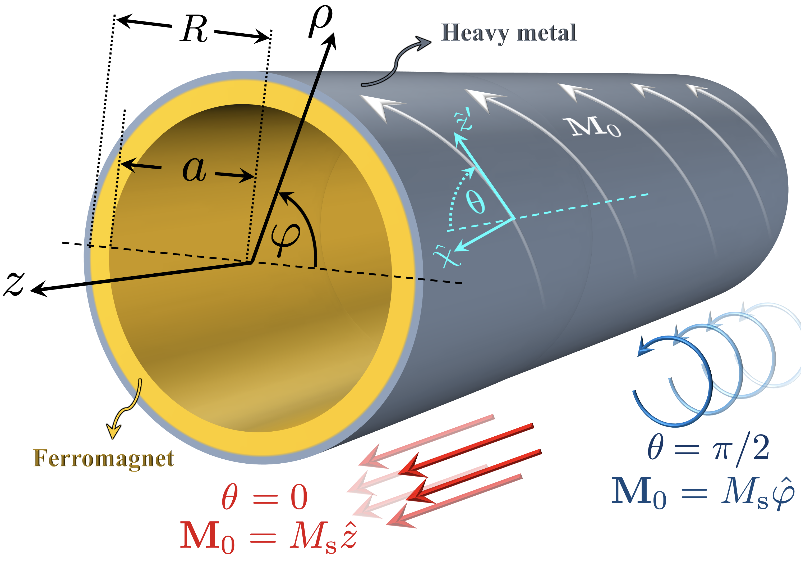
Figure 1: Ferromagnetic nanotube with an equilibrium magnetization $\mathbf{M}_{0}$ describing a curling state. The cylindrical ferromagnet of outer (inner) radius $R$ ($a$) is covered by a heavy-metal layer provoking an interfacial DMI. A glogal reference coordinate system ($\rho$,$\varphi$,$z$) is defined, where $z$ is oriented along the tube axis. A local reference is also defined ($\rho$,$\chi$,$z^{\prime}$), where the equilibrium magnetization $\mathbf{M}_{0}$ points along $\hat{z}^{\prime}$, which makes an angle $\theta$ with the $z$ axis. The cases $\theta=0$ and $\theta=\pi/2$ are illustrated below, which describe an axial and vortex-like configuration, respectively.

A theoretical model is developed to describe the spin-wave dynamics in a nanotube with curling equilibrium magnetization, considering the contributions of Zeeman, exchange interaction, dipolar interaction, radial anisotropy, and the interfacial DMI. While the complete transition from a vortex to a longitudinal magnetized configuration can be theoretically explored, the results of this work will only focus on the limiting cases $\theta=0,\pi/2$. Nevertheless, the expressions for the static and dynamic effective fields and the equilibrium condition are written in a general way for completeness. The temporal evolution of the magnetization is given by the Landau-Lifshitz (LL) equation Gurevich and Melkov (1996),

$$\frac{d\mathbf{M}(\mathbf{r},t)}{dt}=-\mu_{0}\gamma\mathbf{M}(\mathbf{r},t)\times\mathbf{H}^{\rm e}(\mathbf{r},t).$$ (1)

where $\mathbf{M}(\mathbf{r},t)$ is the magnetization, $\mathbf{H}^{\rm e}(\mathbf{r},t)$ the effective magnetic field, and $\gamma$ the gyromagnetic ratio. Considering the wave propagation along the tube axis $z$ and assuming small magnetization deviation, the magnetization and the effective field are, respectively, given by $\mathbf{M}(\mathbf{r},t)=\mathbf{M}_{0}+\mathbf{m}e^{i(kz+l\varphi-\omega t)}$ and $\mathbf{H}^{\rm e}(\mathbf{r},t)=\mathbf{H}^{\rm e0}+\mathbf{h}^{\rm e}e^{i(kz+l\varphi-\omega t)}$, where $|\mathbf{M}_{0}|\gg|\mathbf{m}|$ and $|\mathbf{H}^{\rm e0}|\gg|\mathbf{h}^{\rm e}|$, with $\mathbf{M}_{0}$ being the equilibrium magnetization and $\mathbf{H}^{\rm e0}$ the static effective field. Here, $\omega=2\pi f$ is the angular frequency, $l$ corresponds to an integer number that describes the azimuthal standing wave modes, and $k$ is the axial component of the wave vector. The equilibrium magnetization is considered to be in the direction $\hat{z}^{\prime}=\mathcal{C}\sin\theta\hat{\mathbf{\varphi}}+\cos\theta\hat{z}$. Thus, for $\theta=0$, the magnetization is saturated along the tube axis $z$, and for $\theta=\pi/2$, the magnetization presents a curling or vortex-like equilibrium state, as shown in Fig. 1. The chirality parameter $\mathcal{C}$ has been added to represent the two possible curling orientations, namely $\mathcal{C}=1$ for a right-handed and $\mathcal{C}=-1$ for a left-handed vortex. The effective field contains all the interactions of the system. The magnetic oscillations are described through a local reference system defined by the plane orthogonal to the equilibrium magnetization. Such a coordinate system is constructed by considering that the equilibrium magnetization is orthogonal to the radial direction, i.e., $\hat{\mathbf{\rho}}\cdot\hat{z}^{\prime}=0$. Then, the right-handed orthonormal set is given by $(\hat{\mathbf{\chi}},\hat{\mathbf{\rho}},\hat{z}^{\prime})$, where $\hat{\chi}=\hat{\mathbf{\rho}}\times\hat{z}^{\prime}=-\cos\theta\hat{\mathbf{\phi}}+\mathcal{C}\sin\theta\hat{\mathbf{z}}$. In terms of the magnetization components, the first-order Landau-Lifshitz equation becomes

$$\omega m_{\chi}=i\gamma\mu_{0}(-H^{\rm e0}_{z^{\prime}}m_{\rho}+M_{\text{s}}h^{\rm e}_{\rho})$$ (2a)

$$\omega m_{\rho}=i\gamma\mu_{0}(H^{\rm e0}_{z^{\prime}}m_{\chi}-M_{\text{s}}h^{\rm e}_{\chi}),$$ (2b)

where $M_{\rm s}$ is the saturation magnetization. The dynamic effective field $\mathbf{h}^{\rm e}$ can be written as a linear combination of the dynamic magnetization, $h^{\rm e}_{i}=-\Lambda_{ij}m_{j}$ Gallardo et al. (2022a), where $\Lambda_{ij}$ is the magnetic tensor describing the self-interactions Körber and Kákay (2021). Then, Eqs. (2) result in

$$\omega\begin{pmatrix}m_{\chi}\\ m_{\rho}\end{pmatrix}=i\gamma\mu_{0}M_{\text{s}}\tilde{\mathbf{T}}\begin{pmatrix}m_{\chi}\\ m_{\rho}\end{pmatrix},$$ (3)

with the dynamic matrix

$$\tilde{\mathbf{T}}=\begin{pmatrix}-\Lambda_{\rho\chi}&-\Lambda_{\rho\rho}-\frac{H^{\rm e0}_{z^{\prime}}}{M_{\text{s}}}\\ \Lambda_{\chi\chi}+\frac{H^{\rm e0}_{z^{\prime}}}{M_{\text{s}}}&\Lambda_{\chi\rho}\end{pmatrix}.$$ (4)

By solving this eigenvalue problem, the following dispersion relation is obtained

$$f=\frac{\gamma\mu_{0}M_{\text{s}}}{2\pi}\left[i\Lambda_{\chi\rho}+\sqrt{\left(\frac{H^{\rm e0}_{z^{\prime}}}{M_{\text{s}}}+\Lambda_{\rho\rho}\right)\left(\frac{H^{\rm e0}_{z^{\prime}}}{M_{\text{s}}}+\Lambda_{\chi\chi}\right)}\right],$$ (5)

where, as shown later, it has been considered that $\Lambda_{\rho\chi}=-\Lambda_{\chi\rho}$. Eq. (5) maintains the structure derived in Refs. Cortés-Ortuño and Landeros (2013); Otálora et al. (2016); Gallardo et al. (2022a); Salazar-Cardona et al. (2021), where the elements $\Lambda_{\chi\rho}$ and $\Lambda_{\rho\chi}$ contain the magnetochiral properties, since they depend on the sign of the wave vector $\mathbf{k}$ and the mode index $l$. Nevertheless, it will be shown that such terms also contain the interfacial DMI so that the SW dispersion and azimuthal modes can be nonreciprocal because of exchange, DMI, and dipole-dipole interaction. According to Eq. (5), the $z^{\prime}$ component of the static effective field ($H^{\rm e0}_{z^{\prime}}$) and the linear magnetic tensor elements $\Lambda_{ij}$ are required to describe the SW dynamics of the tubular system. In the following section, these quantities are derived.

II.1 Magnetic effective fields and tensors

The exchange interaction contribution to the effective field is given by $\mathbf{H}^{\text{ex}}=l_{\text{ex}}^{2}\mathbf{\nabla}^{2}\mathbf{M}$, which results in $\mathbf{H}^{\text{ex}0}=\mathcal{C}H_{\text{ex}}\sin\theta\hat{\mathbf{\varphi}}$, and an exchange tensor

$$\tilde{\mathbf{\Lambda}}_{\text{ex}}=\frac{H_{\text{ex}}}{M_{\text{s}}}\left(\begin{array}[]{cc}\cos^{2}\theta+l^{2}+k^{2}R^{2}\beta&i\Delta_{\text{ex}}\\ -i\Delta_{\text{ex}}&1+l^{2}+k^{2}R^{2}\beta\\ \end{array}\right).$$

Here, $H_{\text{ex}}=M_{\text{s}}l_{\text{ex}}^{2}/\beta R^{2}$ and $\Delta_{\text{ex}}=2l\cos\theta$, with $\beta=a/R$, being $R$ and $a$ the outer and inner radii, respectively (see Fig. 1). In this calculation, as in the following ones, an ultrathin nanotube is considered so that some integrals are averaged along the tube thickness. For the effective fields, this is

$$\bar{\mathbf{H}}=\frac{1}{R(1-\beta)}\int_{\beta R}^{R}\mathbf{H}d\rho.$$ (6)

The DM field is derived in Appendix A, where its static part is $\mathbf{H}^{\text{dm}0}=-H_{\text{dm}}\mathcal{C}\sin\theta\hat{\mathbf{\varphi}}$, and the DMI tensor is

$$\tilde{\mathbf{\Lambda}}_{\text{dm}}=\frac{H_{\text{dm}}}{M_{\text{s}}}\begin{pmatrix}\cos^{2}\theta&i\Delta_{\text{dm}}\\ -i\Delta_{\text{dm}}&1\end{pmatrix},$$ (7)

where $H_{\text{dm}}=2D\ln(1/\beta)/[\mu_{0}M_{\text{s}}R(1-\beta)$], $D$ is the Dzyaloshinskii-Moriya strength, and

$$\Delta_{\text{dm}}=l\cos\theta-k\mathcal{C}\sin\theta\frac{R(1-\beta)}{\ln(1/\beta)}.$$ (8)

In flat structures, it is well known that the FM/HM interfaces exhibit a significant perpendicular anisotropy Kim et al. (2017); Samardak et al. (2020); Tacchi et al. (2023). Hence, in the current case, a radial uniaxial anisotropy field is considered, given by $\mathbf{H}^{\rm an}=H_{\rm an}(\mathbf{M}\cdot\hat{\rho})\hat{\rho}$, where ${H}^{\rm an}=2K_{\rho}/\mu_{0}M_{\rm s}$ with $K_{\rho}$ is the radial anisotropy constant. Therefore, the associated tensor is

$$\tilde{\mathbf{\Lambda}}_{\rm an}=-\frac{{H}^{\rm an}}{M_{\rm s}}\begin{pmatrix}0&0\\ 0&1\end{pmatrix}.$$ (9)

For the dipolar contribution, it is noted that $\mathbf{\nabla}\cdot\mathbf{M}_{0}=0$ and $\mathbf{M}_{0}\cdot\hat{\rho}=0$ on the surface of the cylindrical mantle. The surfaces at the tube ends do not contribute Landeros et al. (2009); Mehlin et al. (2018); Vasyukov et al. (2018) because an extended NT along $z$ is assumed. Then, the static dipolar effective field is $\mathbf{H}^{\text{dip}0}=0$. On the other hand, the elements of the dipolar tensor $\tilde{\mathbf{\Lambda}}_{\rm dip}$ are given by (see details in Appendix B),

$$(\tilde{\Lambda}_{\rm dip})_{\chi\chi} =(l\cos\theta-kR_{\text{m}}\mathcal{C}\sin\theta)^{2}\mathcal{I}_{0}$$ (10)

$$(\tilde{\Lambda}_{\rm dip})_{\chi\rho} =-(\tilde{\Lambda}_{\rm dip})_{\rho\chi}=-i\Delta_{\rm dip}$$ (11)

$$(\tilde{\Lambda}_{\rm dip})_{\rho\rho} =\mathcal{I}_{2},$$ (12)

with

$$\Delta_{\rm dip}=(l\cos\theta-kR_{\text{m}}\mathcal{C}\sin\theta)\mathcal{I}_{1}.$$ (13)

Here, an average radius $R_{\text{m}}=R(1+\beta)/2$ has been defined, which comes from the midpoint approach for integration along the radial direction. The functions $\mathcal{I}_{0,1,2}$ are integrals (in $\varphi$) that contain the modified Bessel function of the second kind Gallardo et al. (2022a). These integrals depend on the absolute value of $l$ and $k$ and can only be done numerically for all wave-vector ranges.

For the magnetic configuration $\mathbf{M}_{0}$ to remain stable, the resulting static effective field must align with the equilibrium magnetization. Under this condition, it is required that $\mathbf{H}^{\rm e0}\cdot\hat{\mathbf{\chi}}=0$, which results in the equilibrium condition

$$\mathcal{C}(H_{\text{ex}}+H_{\text{dm}})\cos\theta\sin\theta+H_{\rm ze}\sin(\mathcal{C}\theta-\theta_{\rm ze})=0,$$ (14)

where $\theta_{\rm ze}$ is the angle that the external field makes with respect to the $z$ axis, and $H_{\rm ze}$ is the magnitude of the external field, which is given by $\mathbf{H}^{\rm ze}=H_{\rm ze}[\sin(\mathcal{C}\theta-\theta_{\rm ze})\hat{\mathbf{\chi}}+\cos(\mathcal{C}\theta-\theta_{\rm ze})\hat{z}^{\prime}]$. Note that the external field contains the azimuthal and axial directions in order to favor the condition $\mathbf{M}_{\rm 0}\cdot\hat{\rho}=0$, i.e., the equilibrium magnetization remains in the local $z$-$\varphi$ plane.

II.2 Dispersion relation and frequency nonreciprocity

With the dispersion relation shown in Eq. (5) in terms of the effective field and magnetic tensor elements specified in the previous section, the SW frequency becomes

$$f=\frac{\gamma\mu_{0}}{2\pi}\left[(M_{\text{s}}\Delta_{\rm{dip}}-H_{\text{ex}}\Delta_{\rm{ex}}-H_{\text{dm}}\Delta_{\rm{dm}})+\sqrt{\left(H^{\rm e0}_{z^{\prime}}+M_{\rm s}\Lambda_{\rho\rho}\right)\left(H^{\rm e0}_{z^{\prime}}+M_{\rm s}\Lambda_{\chi\chi}\right)}\right],$$ (15)

where

$$H^{\rm e0}_{z^{\prime}}=H_{\rm ze}\cos(\theta-\theta_{\rm ze})-(H_{\rm{ex}}+H_{\rm{dm}})\sin^{2}\theta,$$ (16)

and the diagonal tensor elements $\Lambda_{\rho\rho}$ and $\Lambda_{\chi\chi}$ can be obtained from the contributing tensors in section II.1. In this case, the only terms that change sign under wave vector inversion are $\Lambda_{\chi\rho}$ and $\Lambda_{\rho\chi}$, which satisfy the condition $\Lambda_{\rho\chi}=-\Lambda_{\chi\rho}$. The frequency difference under wave vector inversion is $\Delta f=f(\mathbf{k})-f(-\mathbf{k})=f(k,l)-f(-k,-l)$, and then the frequency shift is given by:

$$\Delta f=\frac{\gamma\mu_{0}}{\pi}(M_{\text{s}}\Delta_{\rm{dip}}-H_{\text{ex}}\Delta_{\rm{ex}}-H_{\text{dm}}\Delta_{\rm{dm}}),$$ (17)

which can be separated into terms proportional to the axial ($k$) and azimuthal ($l/R$) wave vectors, $\Delta f=\Delta f_{k}+\Delta f_{l}$, where

$$\Delta f_{k}=\frac{\mu_{0}\gamma}{\pi}kM_{\text{s}}\mathcal{C}\sin\theta\left(\frac{2D}{\mu_{0}M^{2}_{\text{s}}}-R_{\text{m}}\mathcal{I}^{(k,l)}_{1}\right)$$ (18)

and

$$\Delta f_{l}=\frac{\mu_{0}\gamma}{\pi}\frac{l}{R}M_{\text{s}}\cos\theta\left(R\mathcal{I}^{(k,l)}_{1}-\frac{2D}{\mu_{0}M^{2}_{\text{s}}}\frac{\ln(1/\beta)}{(1-\beta)}-\frac{2l_{\text{ex}}^{2}}{\beta R}\right).$$ (19)

In Eq. (18), it is noted that the dipolar and DM interactions induce asymmetry in the SW bandstructure for waves propagating along the tube axis. For zero DMI, the frequency shift is generated only by the dipole-dipole interaction, which is in concordance with previous results. Otálora et al. (2016); Sheka et al. (2020); Gallardo et al. (2022a); Salazar-Cardona et al. (2021); Körber et al. (2022). It is important to note that the function $\mathcal{I}^{(k,l)}_{1}$ depends on the absolute value of the mode index $l$, making the frequency shift $\Delta f_{k}$ different for $l=0$ and $l\neq 0$. On the other hand, the frequency shift $\Delta f_{l}$ [see Eq. (19)] evidences the chiral features of the azimuthal standing waves. One can see that dipolar, exchange, and DMI contribute to azimuthal chiral effects. Namely, the circumferential standing waves will differ for $+l$ and $-l$ as long as $\theta\neq\pi/2$. The role of exchange and dipolar interactions for $\theta\neq\pi/2$ has previously been studied Salazar-Cardona et al. (2021). However, the role of the Dzyaloshinskii-Moriya interaction has not been considered until now.

From Eq. (19), it can be concluded that the exchange contribution affects the azimuthal asymmetry in the same way as the Dzyaloshinskii–Moriya interaction. Indeed, a simple analysis allows obtaining an effective parameter

$$D_{\rm ex}=\frac{2A_{\rm ex}}{\beta R}\frac{1-\beta}{\ln{1/\beta}}.$$ (20)

Thus, for the azimuthal frequency shift, the exchange and DM interactions can be combined into an effective constant $D_{\rm eff}=D+D_{\rm ex}$. In the limit $R\rightarrow\infty$, it is clear that $D_{\rm ex}=0$ because the magnetochirality induced by exchange requires a finite curvature Sheka et al. (2020); Salazar-Cardona et al. (2021). On the other hand, in the same limit $R\rightarrow\infty$, $\ln(1/\beta)/(1-\beta)\rightarrow 1$, $1/R^{2}\rightarrow 0$ and $\mathcal{I}^{(k,l)}_{1}\rightarrow 0$. Hence, using the relation $k_{\varphi}=l/R$, the frequency shift becomes $\Delta f_{l}=(2\gamma/\pi M_{\rm s})Dk_{\varphi}$, which, at $\theta=0$, corresponds to the frequency shift obtained for DE waves propagating in a planar FM/HM structure Melcher (1973); Costa et al. (2010); Cortés-Ortuño and Landeros (2013); Moon et al. (2013); Di et al. (2015b); Cho et al. (2015); Stashkevich et al. (2015); Tacchi et al. (2017); Gallardo et al. (2019c); Kuepferling et al. (2023). In the case $\theta=\pi/2$, the contribution of the DMI in the nonreciprocity is given by $\Delta f_{k}=\mathcal{C}\frac{2\gamma}{\pi M_{\text{s}}}Dk$, which also coincides with that for DE modes in planar systems. It is worth noting that, in the general case, the dipolar terms $\mathcal{I}^{(k,l)}_{1}$ depend on the magnitude of $k$ and are the only contribution to the frequency nonreciprocity that is nonlinear with $k$.

Figure 2: Spin-wave dispersions for $D=-1\ \rm mJ/m^{2}$ (red), $D=0$ (black) and $D=1\ \rm mJ/m^{2}$ (blue). In (a) and (b), the equilibrium magnetization presents a vortex-like ground state ($\theta=\pi/2$), where the case $l=0$ [$l=\pm 1$] is illustrated in (a) [(b)]. In (c) and (d), the nanotube is saturated with an external field applied along its axis ($\theta=0$), where the cases (c) $l=0$ and (d) $l=\pm 1$ are depicted. The bottom scheme in (c) describes the dynamic magnetization for the dynamic state $l=0$. The directions of vectors $\mathbf{m}_{i}\times\mathbf{m}_{j}$, with $\mathbf{m}_{i,j}$ being the dynamic magnetization components, and the DM vector (for $D>0$ and $D<0$) are illustrated.

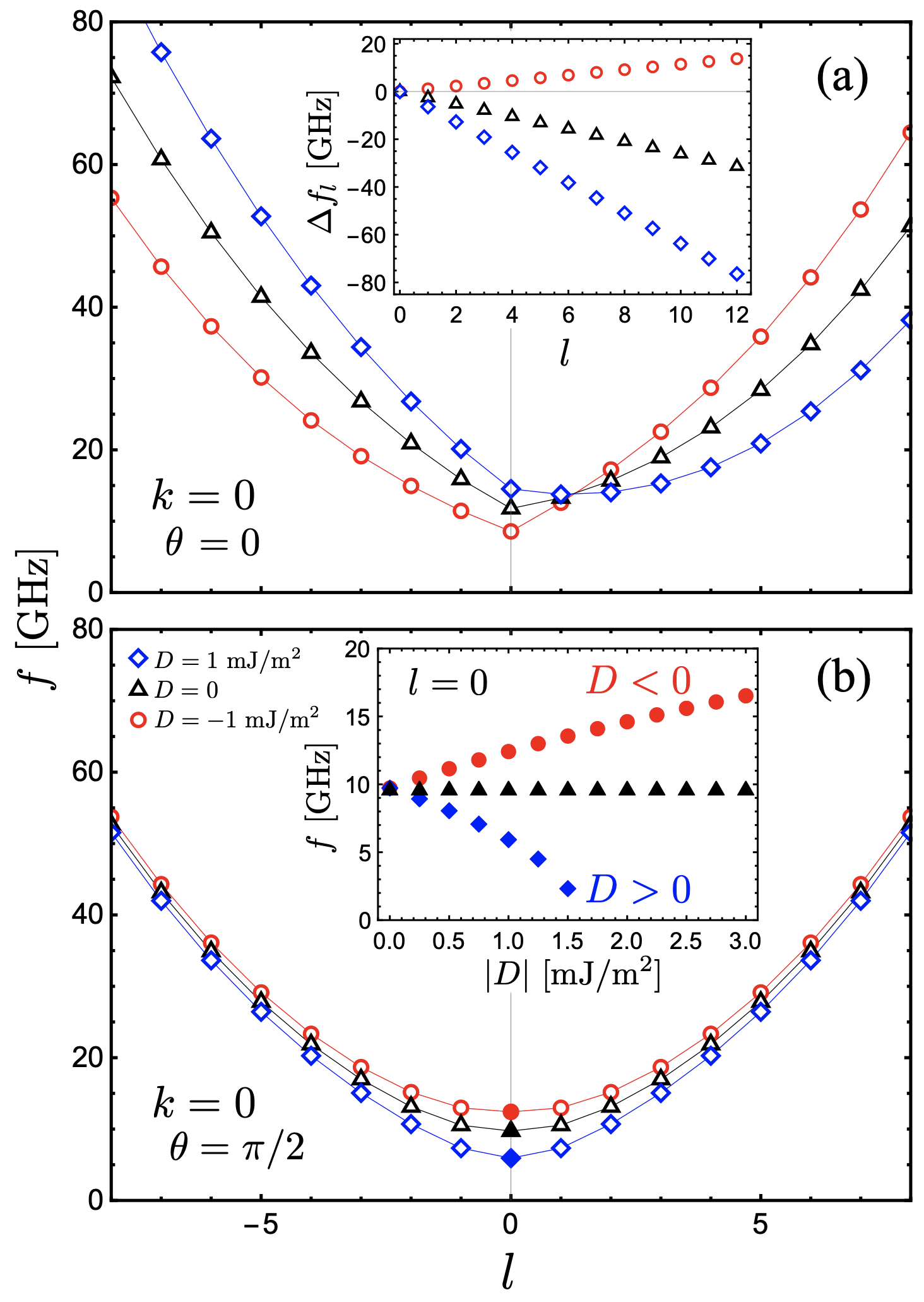
Figure 3: Spin-wave frequency as a function of the azimuthal mode index $l$ for $k=0$. Diamonds, triangles, and circles depict the cases $D=1$ mJ/m², $D=0$, and $D=-1$ mJ/m², respectively. In (a), a saturated equilibrium state along $z$ is considered ($\theta=0$), where the inset shows the frequency shift $\Delta f_{l}$ for the cases $D=0$ and $D=1\pm$ mJ/m². The circumferential equilibrium state ($\theta=\pi/2$) is assumed in (b), where the frequency against the magnitude of the Dzyaloshinskii-Moriya constant $D$ is shown in its inset for $l=0$ (solid markers).

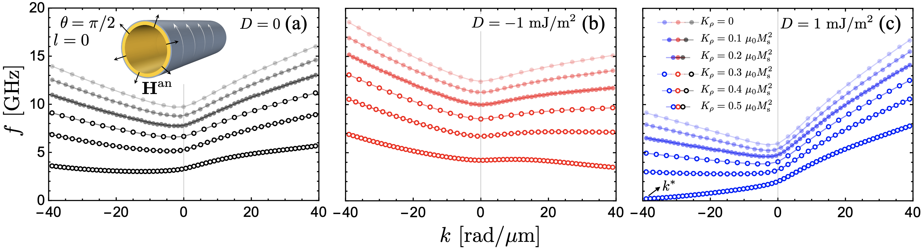
Figure 4: Spin-wave dispersions calculated for (a) $D=0$, (b) $D=-1\ \rm mJ/m^{2}$, and (c) $D=1\ \rm mJ/m^{2}$ (blue). In all cases, the vortex-like equilibrium state ($\theta=\pi/2$) and $l=0$ are considered. The plots are calculated for different values of the radial anisotropy constant $K_{\rho}$, as depicted in (c). The filled circles consider the cases $K_{\rho}=0$, $K_{\rho}=0.1\ \mu_{0}M_{\rm s}^{2}$, and $K_{\rho}=0.2\ \mu_{0}M_{\rm s}^{2}$. While the open circles are calculated for $K_{\rho}=0.3\ \mu_{0}M_{\rm s}^{2}$, $K_{\rho}=0.4\ \mu_{0}M_{\rm s}^{2}$, and $K_{\rho}=0.5\ \mu_{0}M_{\rm s}^{2}$. In (c), the wave vector $k^{*}$, at which the frequency becomes zero, is highlighted.

II.3 Small wave-vector approximation

Analytical expressions for the integrals $\mathcal{I}^{(k,l)}_{i}$ can be derived at the small wave-vector limit. Such expressions are obtained up to zeroth order in Appendix B. By focusing on the frequency asymmetry, the frequency shift at $k\rightarrow 0$ becomes

$$\Delta f_{k}^{k\rightarrow 0}\approx\frac{\mu_{0}\gamma}{\pi}kM_{\text{s}}\mathcal{C}\sin\theta\left(\frac{2D}{\mu_{0}M^{2}_{\text{s}}}+\frac{R-a}{2}\delta_{l,0}\right).$$ (21)

Note that for $l=0$, the DM and dipolar couplings induce frequency nonreciprocity. Nonetheless, for $l\neq 0$, the frequency asymmetry is due to only DMI because, in this case, $\mathcal{I}^{(k,l)}_{1}(k\rightarrow 0)=0$. Also, for $D=0$, Eq. (21) coincides with Eq. (18) of Ref. Gallardo et al. (2022a) when the equilibrium magnetization is in a circumferential vortex state ($\theta=\pi/2$).

On the other hand, the small-$k$ approximation for the frequency asymmetry associated with the azimuthal standing waves is

$$\Delta f_{l}^{k\rightarrow 0}\approx-\frac{\mu_{0}\gamma}{\pi}\frac{l}{R}M_{\text{s}}\cos\theta\left(\frac{2D\ln(1/\beta)}{\mu_{0}M^{2}_{\text{s}}(1-\beta)}+\frac{2l_{\text{ex}}^{2}}{\beta R}\right).$$ (22)

Hence, in the limit $k\rightarrow 0$, only the exchange interaction and DMI induce magnetochirality if $l\neq 0$. In other words, Eq. (22) suggests that the asymmetry of azimuthal standing waves is predominantly due to the exchange interaction and DMI, and the dipolar interaction plays a minor role. Nonetheless, it is worth noticing that only the dipolar interaction can induce nonlinear effects in the frequency shift, as evidenced in the inset of Fig. 2(a). This effect is explained by the dependence of the integral $\mathcal{I}^{(k,l)}_{1}$ on $k$, which is lost in the zeroth order approximation considered in Eqs. (21) and (22) and higher order terms are needed. Note that these analytical expressions [Eqs. (21) and (22)] account for asymmetry in both $k$ and $l$, providing insights into the role of curvature and the various interactions in SW dynamics.

III Results

In the subsequent discussion, magnetic parameters for Permalloy (Ni₈₀Fe₂₀) are used for the calculations, namely $M_{\rm{s}}=796$ kA/m and $l_{\rm{ex}}=5.7$ nm (equivalent to an exchange constant $A_{\rm{ex}}=13$ pJ/m). The gyromagnetic ratio is $\gamma=175.929$ GHz/T. In addition, the geometrical parameters of the tubular system are $R=40$ nm and $a=35$ nm, so the NT thickness is 5 nm.

Fig. 2 shows the spin-wave dispersion for the cases (a-b) $\theta=\pi/2$ and (c-d) $\theta=0$, evaluated for $K_{\rho}=0$. To stabilize saturated and vortex-like equilibrium states, it is assumed that an external field of magnitude $\mu_{0}H_{\rm ze}=130$ mT is applied along the local $z^{\prime}$ direction, ensuring $\theta=\theta_{\rm ze}$, with $\theta_{\rm ze}=0$ for the saturated state and $\theta_{\rm ze}=\pi/2$ for the circumferential equilibrium configuration. Fig. 2(a) displays the dispersion at $\theta=\pi/2$, for $D=-1~\mathrm{mJ/m^{2}}$ (red), $D=0$ (black), and $D=1~\mathrm{mJ/m^{2}}$ (blue). The asymmetry in the SW dispersion at $D=0$ arises from the dynamic dipolar interaction, which causes counterpropagating waves to have different wavelengths at the same frequency Otálora et al. (2016); Sheka et al. (2020); Gallardo et al. (2022a); Salazar-Cardona et al. (2021); Körber et al. (2022). As indicated by Eq. (18), the exchange interaction does not contribute to this frequency asymmetry. When the DMI is active, the dispersive SW properties are modified depending on the sign of $D$ and the helicity of the curling magnetization. For a counterclockwise ($\mathcal{C}=1$) vortex magnetization and for $D>0$, the DMI reinforces the asymmetry induced by the dipolar interaction, whereas for $D<0$, the DMI opposes the dipolar-induced asymmetry. This results in a negative frequency shift $\Delta f_{k}$, as illustrated in the inset of Fig. 2(a). For the states $l=\pm 1$ (at $\theta=\pi/2$), the azimuthal standing waves are degenerate in frequency because $\Delta f_{l}=0$. This result holds for any $l\neq 0$. Specifically, the SW dispersion depends on the magnitude of $l$ [see Fig. 2(b)]. In this case, the frequency asymmetry (see inset) differs from the case where $l=0$. This behavior is attributed to the dipolar interaction, where the dependence of $\Delta f_{k}$ on $l$ is determined by the integral $\mathcal{I}_{1}$ in Eq. (18). The analytical expression in Eq. (21), evaluated at small wave vectors, explicitly reveals this dependence. Indeed, at $D=0$, the frequency shift tends to zero in the limit $k\rightarrow 0$, as shown in the inset of Fig. 2(b).

For the saturated case ($\theta=0$), the SW dispersion is symmetric because $\Delta f_{k}\propto\sin\theta$. Neither dipolar interactions nor DMI induce nonreciprocity with respect to $k$, as shown in Figs. 2(c) and 2(d). Nevertheless, in this configuration, the DMI shifts the magnon frequency depending on the sign of $D$. As illustrated in the scheme at the bottom of Fig. 2(c), the sign of the Dzyaloshinskii-Moriya constant $D$ determines whether the DM energy $\epsilon_{\mathrm{dm}}$ is maximized or minimized. For $D>0$, $\epsilon_{\mathrm{dm}}\propto\mathbf{D}\cdot(\mathbf{m}_{i}\times\mathbf{m}_{j})$ reaches a maximum because $\mathbf{D}$ and the dynamic vector spin chirality $\mathbf{m}_{i}\times\mathbf{m}_{j}$ are parallel Grohol et al. (2005); Onoda and Nagaosa (2007); Menzel et al. (2012); Ishizuka and Nagaosa (2018). Conversely, for $D<0$, $\mathbf{D}$ points out of the page, resulting in $\mathbf{D}\cdot(\mathbf{m}_{i}\times\mathbf{m}_{j})<0$, which reduces $\epsilon{{}_{\mathrm{dm}}}$. Consequently, the frequency decreases (increases) for $D<0$ ($D>0$). In Fig. 2(d), it is evident that the modes depend on the sign of $l$, unlike the vortex-like case. This dependence is associated with the finite frequency shift $\Delta f_{l}$ that is maximized for $\theta=0$, where dipolar, exchange, and DMI interactions contribute to a dependence proportional to $l\cos\theta$, as derived in Eq. (19).

The asymmetry associated with the azimuthal index $l$ is further analyzed in Fig. 3, where the frequency as a function of $l$ is plotted for zero axial wave vector. In Fig. 3(a), the three cases $D=-1\ \rm mJ/m^{2}$ (circles), $D=0$ (triangles), and $D=1\ \rm mJ/m^{2}$ (diamonds) are shown for an equilibrium magnetization aligned along the tube axis $\theta=0$. It is observed that in this configuration, the curve at $D=0$ exhibits a degree of nonreciprocity concerning the change in sign of $l$, wherein the frequency minimum occurs at positive values [$l=1$ in Fig. 3(a)]. This behavior is consistent with previously reported results Salazar-Cardona et al. (2021), where this asymmetry is induced by dipolar and exchange interactions, as described in Eq. (19). When the interfacial DMI is included, the frequency asymmetry is enhanced for $D>0$, shifting the minimum to higher values of $l$. Conversely, for $D<0$, the frequency minimum shifts to negative $l$ values. As illustrated in the inset of Fig. 3(a), the deviation of $\Delta f_{l}$ around the $D=0$ curve (triangles) is symmetric for positive and negative values of $D$, namely $|\Delta f_{l}(D>0)-\Delta f_{l}(D=0)|=|\Delta f_{l}(D<0)-\Delta f_{l}(D=0)|$. This behavior is associated with the term in $\Delta f_{l}$ that is linear with $D$.

In the vortex configuration ($\theta=\pi/2$), the frequency depends on the magnitude of $l$, resulting in a symmetric behavior against $l$, as shown in Fig. 3(b). The parabolic dependence highlights the dominance of the exchange interaction, which scales as $\sim l^{2}$. Similar to the saturated case, the DMI either increases or decreases the frequencies depending on the sign of $D$. This is further demonstrated in the inset of Fig. 3(b), where the frequency at $l=0$ is plotted as a function of $|D|$. As the magnitude of $D$ increases, the modes for $D<0$ increase their frequency, while those for $D>0$ are excited at a lower frequency. Indeed, for $D\approx 1.6\ \rm mJ/m^{2}$, the frequency is close to zero, leading to the emergence of soft (or Goldstone) modes indicating the destabilization of the equilibrium state Leaf et al. (2006); Montoncello et al. (2007); Ríos-Venegas et al. (2022); Grassi et al. (2022); Kisielewski et al. (2023). If a given mode with $l\neq 0$ reaches zero frequency before the mode at $l=0$, the new ground state is expected to exhibit a magnetic texture with an azimuthal modulation determined by $l$. The analysis of different ground states in tubular systems with Dzyaloshinskii-Moriya interaction is beyond the scope of this work and will be addressed in a forthcoming publication Mimica-Figari et al. (2025).

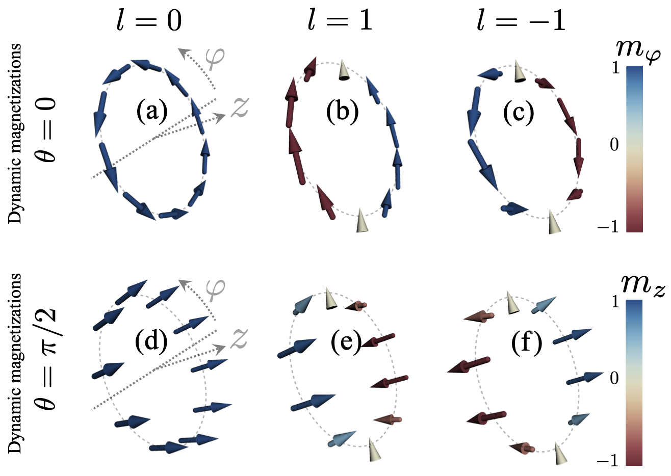
Figure 5: Dynamic magnetization calculated for $D=0$ and $K_{\rho}=0$. In (a)-(c), the dynamic magnetizations as a function of $\varphi$ are shown for the dynamic states $l=0,\pm 1$ with $\theta=0$. In (d)-(f), the vortex-like configuration is illustrated ($\theta=\pi/2$) where the dynamic magnetization are evaluated for $l=0,\pm 1$.

The impact of radial anisotropy is illustrated in Fig. 4, where the spin-wave dispersion is analyzed for $l=0$, $\theta=\pi/2$, and varying values of the anisotropy constant $K_{\rho}$. Dispersion curves are presented for three cases: $D=0$, $D=-1\ \rm mJ/m^{2}$, and $D=1\ \rm mJ/m^{2}$, corresponding to Figs. 4(a), 4(b), and 4(c), respectively. For $D=0$, the dispersion curves reveal a progressive reduction in frequency as $K_{\rho}$ increases, while the frequency shift ($\Delta f_{k}$) remains unaffected by changes in anisotropy. A notable feature is the shift of the dispersion minimum to a finite wave vector $k^{*}$, indicating the existence of a critical anisotropy constant $K^{*}_{\rho}$ where the frequency becomes zero, i.e., $f(k^{*})=0$. Beyond this critical anisotropy value, the nanotube is predicted to develop a textured ground state with periodicity along the $z$ axis, characterized by a wavelength $\lambda=2\pi/k^{*}$. This idea aligns with results obtained in other systems Leaf et al. (2006); Montoncello et al. (2007); Ríos-Venegas et al. (2022); Grassi et al. (2022); Kisielewski et al. (2023), where the critical wave vector $k^{*}$ enables the prediction of a periodic magnetic texture. In Fig. 4(a), for $D=0$, the minimum occurs at $k^{*}<0$, reflecting the chiral properties inherent to the emerging magnetic texture. When the DMI is introduced, the $f(k^{*})=0$ state is observed at $k^{*}>0$ for $D=-1\ \rm mJ/m^{2}$, and at $k^{*}<0$ for $D=1\ \rm mJ/m^{2}$, as shown in Figs. 4(b) and 4(c), respectively. For the specific case of $D=1\ \rm mJ/m^{2}$ and $K_{\rho}=0.5\ \mu_{0}M_{\rm s}^{2}$, which means that radial anisotropy and dipolar fields are balanced, the zero-frequency state is nearly reached at $k^{*}=-40$ rad/$\mu$m, suggesting the formation of a magnetic texture with a similar pitch vector, as occurs in planar films Ríos-Venegas et al. (2022); Grassi et al. (2022); Kisielewski et al. (2023).

The periodic equilibrium states of thin films with DMI have been previously reported Ríos-Venegas et al. (2022). In this context, the predicted textures in nanotubes based on dynamic aspects align with results reported in Ref. Yershov et al., 2020, where periodic equilibrium states are observed at a critical value of the DM constant. This dynamic prediction of periodic magnetic textures under critical conditions is nontrivial. Intuitively, one might expect that increasing anisotropy would stabilize a purely radial magnetization orientation in the nanotube. However, the results demonstrate that even for $D=0$, the tube exhibits a texture with a periodic radial component, where the chirality arises from dipolar interactions. For dynamic states evaluated at $l\neq 0$, a similar trend to that discussed in Fig. 4 is observed (not shown). In the saturated state, anisotropy also reduces the frequency of the modes. However, in this case, the frequency minima occur at zero wave vector, indicating that anisotropy uniformly enhances the radial component of the equilibrium magnetization across the entire nanotube.

Finally, the spin-wave profiles are calculated for $D=0$ and $K_{\rho}=0$. Fig. 5 illustrates the normalized dynamic magnetization (in arbitrary units) for the dynamic states $l=0,\pm 1$. The dynamic magnetization component in the tube mantle is highlighted using a color code. For $l=0$, the dynamic magnetization is shown in Fig. 5(a), exhibiting the same amplitude along the $\varphi$-direction. In contrast, the case $l=1$ [see Fig. 5(b)] presents an almost uniform dynamic state, where the dynamic magnetization tends to align in a given direction. This configuration clearly implies a reduction in the exchange energy, as it promotes a parallel orientation of the magnetic moments. By comparing the state $l=1$ with the one illustrated in Fig. 5(c) ($l=-1$), it is seen that the dynamic energies are different, with the configuration $l=-1$ being more energetic than $l=1$. This observation explains the asymmetry of the exchange energy evident in Fig. 3(a) (see black triangles).

When the DMI is included, for the case $\theta=0$, the energy in the configuration $l=-1$ is either reduced or increased depending on the sign of $D$. For $D>0$, the direction of the DM vector $\mathbf{D}$ between two neighboring spins across the nanotube’s perimeter is determined by $+\hat{z}$, while the product $\mathbf{m}_{i}\times\mathbf{m}_{j}$ in the configuration shown in Fig. 5(c) also points along $+z$. Consequently, the dynamic energy (or frequency) increases for the case $l=-1$, as the DM energy [$\epsilon_{\rm dm}\propto\mathbf{D}\cdot(\mathbf{m}_{i}\times\mathbf{m}_{j})$] increases. In contrast, for $D<0$, the dynamic DM energy becomes negative, and thus, the state with $l=-1$ becomes less energetic than the state with $l=1$, consistent with the results shown in Fig. 3(a) (see red open circles). It is worth mentioning that the dynamic magnetization vectors illustrated in Figs. 5(a)–(c) are slightly modified in the presence of DMI, at least within the range $|D|<1$ mJ/m². Therefore, although the states illustrated in Fig. 5 are not equivalent under the presence of DMI, they allow understanding why the frequency of the modes increases or decreases when DMI is active. In the vortex configuration ($\theta=\pi/2$), the state $l=0$ [see Fig. 5(d)] exhibits a dynamic magnetization distribution with the same amplitude along the $\varphi$-direction, as in the case $\theta=0$. In this configuration, the magnetization component $m_{z}$ lies along the tube mantle. The cases $l=\pm 1$ are shown in Figs. 5(e)–(f), where the dynamic energy is identical for these states. This result implies that the frequencies of states with negative and positive $l$ are equal, thereby supporting the results presented in Fig. 3(b).

IV Summary

The theoretical study provides a detailed analysis of spin-wave dynamics in nanotubes, emphasizing the crucial roles of Dzyaloshinskii-Moriya interaction and curvature. It is shown that nonreciprocity in spin-wave propagation is a key characteristic of these systems, arising from a combination of exchange, DMI, and dipolar interactions. In the vortex-like configuration, a frequency nonreciprocity is observed wherein, for a positive DM constant, the DMI reinforces the asymmetry induced by the dipolar interaction, while in the contrary case, the asymmetry caused by the DMI is opposed to the dipolar one. In a longitudinal magnetization state, the exchange and DM interactions predominantly lead to chiral effects in the SW bandstructure for azimuthal standing waves. In contrast, propagation along the tube axis is reciprocal in frequency. Under the inclusion of a radial anisotropy, it is found that it reduces the frequency of the modes and shifts the dispersion minimum to a finite wave vector for the vortex state. For the saturated state, the frequency minima occurs at zero wave vector. The properties of the spin-wave modes are close to zero frequency, which allows for the prediction of the emergence of chiral magnetic textures. The insights from this work can be applied to the development of three-dimensional chiral magnetic nanostructures, offering new possibilities for magnonics and nanoscale information processing.

Appendix A Effective Dzyaloshinskii-Moriya field

The effective Dzyaloshinskii-Moriya field must be carefully calculated to incorporate curvature effects. In cylindrical geometry, the interfacial DM energy term is expressed as Mancilla-Almonacid et al. (2020),

$$E_{\text{dm}}(\mathbf{M})=\frac{D}{M_{\text{s}}^{2}}\int_{\Omega}\hat{\mathbf{\rho}}\cdot[(\mathbf{M}(\mathbf{\nabla}\cdot\mathbf{M})-(\mathbf{M}\cdot\mathbf{\nabla})\mathbf{M}]dV.$$ (23)

Due to the non-commutativity between the unit vector $\hat{\mathbf{\rho}}$ and the operator $\mathbf{\nabla}$, curvature-induced terms naturally emerge in the effective DMI field. This field can be obtained by calculating the functional derivative of the energy with respect to the magnetization. This is

$$\delta E_{\rm dm}(\mathbf{M},\mathbf{v}) \equiv\lim_{\epsilon\to 0}\frac{E_{\rm dm}(\mathbf{M}+\epsilon\mathbf{v})-E_{\rm dm}(\mathbf{M})}{\epsilon}$$

$$=\int_{\Omega}\frac{\delta\epsilon_{\rm dm}}{\delta\mathbf{M}}\cdot\mathbf{v}dV$$ (24)

for an arbitrary vector $\mathbf{v}$. Then, the effective DM field is

$$\mathbf{H}^{\text{dm}}=-\frac{1}{\mu_{0}}\frac{\delta\epsilon_{\text{dm}}}{\delta\mathbf{M}},$$ (25)

with $\epsilon_{\rm{dm}}$ being the DM energy density ($\epsilon_{\rm dm}=\partial E_{\rm{dm}}/\partial V$). After some algebraic manipulations, the following expression for the effective field is obtained:

$$\mathbf{H}^{\text{dm}}=-\frac{2D}{\mu_{0}M^{2}_{\text{s}}}\left(\hat{\mathbf{\rho}}(\mathbf{\nabla}\cdot\mathbf{M})-\mathbf{\nabla}(\hat{\mathbf{\rho}}\cdot\mathbf{M})+\frac{M_{\varphi}\hat{\mathbf{\varphi}}}{\rho}\right).$$ (26)

Note that a thin nanotube is considered in this work. Therefore, the expression for a surface contribution in Eq. (24) has been omitted. Finally, by considering the dynamic and static magnetization components, it is easy to obtain $\mathbf{H}^{\text{dm}0}=-H_{\text{dm}}\sin\theta\hat{\mathbf{\varphi}}$ and $\mathbf{h}^{\text{dm}}=-\tilde{\mathbf{\Lambda}}_{\text{dm}}\mathbf{m}$, where matrix $\tilde{\mathbf{\Lambda}}_{\text{dm}}$ is given in Eq. (7).

Appendix B Effective dipolar field

The dipolar field is derived in a manner similar to that described by Alvarado et al. Alvarado-Seguel and Gallardo (2019). The dipolar effective field can be obtained as $\mathbf{H}^{\text{dip}}=-\mathbf{\nabla}\Phi(\mathbf{r},t)$, where the magnetostatic potential $\Phi$ is given by

$$\Phi(\mathbf{r},t)=-\int_{\Omega}\frac{\mathbf{\nabla}^{\prime}\cdot\mathbf{M}(\mathbf{r}^{\prime},t)}{4\pi|\mathbf{r}-\mathbf{r}^{\prime}|}dV^{\prime}+\int_{\partial\Omega}\frac{\hat{\mathbf{n}}^{\prime}\cdot\mathbf{M}(\mathbf{r}^{\prime},t)}{4\pi|\mathbf{r}-\mathbf{r}^{\prime}|}dS^{\prime}.$$ (27)

By considering the magnetization described in section II, the volumetric and surface magnetic charges are

$$\mathbf{\nabla}\cdot\mathbf{M}=\left[\frac{m_{\rho}}{\rho}+i\left(k\sin\theta-\frac{l\cos\theta}{\rho}\right)m_{\chi}\right]e^{i(kz+l\phi-\omega t)}$$ (28)

and

$$\mathbf{n}\cdot\mathbf{M}=\pm m_{\rho}e^{i(kz+l\phi-\omega t)},$$ (29)

respectively. Therefore, the tensor elements of $\tilde{\mathbf{\Lambda}}_{\rm dip}$ are

$$(\Lambda_{\rm dip})_{\chi\chi} =\iiint(l\cos\theta-k\rho\sin\theta)(l\cos\theta-k\rho^{\prime}\sin\theta)\frac{1}{\rho}G_{0}(\rho,\rho^{\prime},\varphi^{\prime})d\rho d\rho^{\prime}d\varphi^{\prime}$$ (30a)

$$(\Lambda_{\rm dip})_{\chi\rho} =-i\iiint\left(l\cos\theta-k\rho\sin\theta\right)\frac{\rho^{\prime}}{\rho}G_{1}(\rho^{\prime},\rho,\varphi^{\prime})d\rho d\rho^{\prime}d\varphi^{\prime}$$ (30b)

$$(\Lambda_{\rm dip})_{\rho\chi} =i\iiint(l\cos\theta-k\rho^{\prime}\sin\theta)G_{1}(\rho,\rho^{\prime},\varphi^{\prime})d\rho d\rho^{\prime}d\varphi^{\prime}$$ (30c)

$$(\Lambda_{\rm dip})_{\rho\rho} =\iiint\rho^{\prime}G_{2}(\rho,\rho^{\prime},\varphi^{\prime})d\rho d\rho^{\prime}d\varphi^{\prime}$$ (30d)

where,

$$G_{0}(\rho,\rho^{\prime},\varphi^{\prime}) =\frac{e^{il\varphi^{\prime}}}{2\pi R(1-\beta)}K_{0}\left(|k|\sqrt{\rho^{2}+\rho^{\prime 2}-2\rho\rho^{\prime}\cos\varphi^{\prime}}\right)$$ (31a)

$$G_{1}(\rho,\rho^{\prime},\varphi^{\prime}) =\partial_{\rho}G_{0}(\rho,\rho^{\prime},\varphi^{\prime})$$ (31b)

$$G_{2}(\rho,\rho^{\prime},\varphi^{\prime}) =\partial_{\rho\rho^{\prime}}G_{0}(\rho,\rho^{\prime},\varphi^{\prime}).$$ (31c)

Here, $K_{0}$ is the zeroth modified Bessel function of the second kind. The integrals given in Eq. (30) must be solved numerically. Notice that, unlike exchange and DM dynamic tensors, the dipolar interaction has the condition $(\Lambda_{\rm dip})_{\rho\chi}\neq-(\Lambda_{\rm dip})_{\chi\rho}$. Nevertheless, because a very thin nanotube is considered, the integrals in $\rho$ and $\rho^{\prime}$ can be approximated as $\int_{0}^{d}F(x)dx\approx dF(d/2)$. Thus,

$$(\tilde{\Lambda}_{\rm dip})_{\chi\chi} =(l\cos\theta-kR_{\text{m}}\sin\theta)^{2}\mathcal{I}^{(k,l)}_{0}$$ (32a)

$$(\tilde{\Lambda}_{\rm dip})_{\chi\rho} =-i(l\cos\theta-kR_{\text{m}}\sin\theta)\mathcal{I}^{(k,l)}_{1}$$ (32b)

$$(\tilde{\Lambda}_{\rm dip})_{\rho\rho} =\mathcal{I}^{(k,l)}_{2},$$ (32c)

and $(\tilde{\Lambda}_{\rm dip})_{\rho\chi}=-(\tilde{\Lambda}_{\rm dip})_{\chi\rho}$. Here, $R_{\text{m}}=R(1+\beta)/2$ is the midpoint between the internal and external radius of the tube. The integrals $\mathcal{I}^{(k,l)}_{0,1,2}$ become

$$\mathcal{I}^{(k,l)}_{0} =R^{2}(1-\beta)^{2}\int\frac{1}{R_{\text{m}}}G_{0}(R_{\text{m}},R_{\text{m}},\varphi^{\prime})d\varphi^{\prime}$$ (33a)

$$\mathcal{I}^{(k,l)}_{1} =R^{2}(1-\beta)^{2}\int G_{1}(R_{\text{m}},R_{\text{m}},\varphi^{\prime})d\varphi^{\prime}$$ (33b)

$$\mathcal{I}^{(k,l)}_{2} =R^{2}(1-\beta)^{2}\int R_{\text{m}}G_{2}(R_{\text{m}},R_{\text{m}},\varphi^{\prime})d\varphi^{\prime}.$$ (33c)

These expressions require numerical integration on the azimuthal angle $\varphi^{\prime}$. Nevertheless, these integrals can be analytically calculated in the case of small wave vectors. The series expansion of the Bessel function is used $K_{0}(x)=-\gamma-\ln(x/2)$, where $\gamma$ is the Euler-Mascheroni constant. Such a small $k$ approach allows for an analytical solution of the $\varphi^{\prime}$ coordinate integration using the residue theorem. An integral of the form,

$$I=\int_{0}^{2\pi}f(\sin\varphi^{\prime},\cos\varphi^{\prime})d\varphi^{\prime}$$ (34)

can be solved by using the change of variable $z=e^{i\varphi^{\prime}}$. The result is computed by calculating the residues inside the unit circle,

$$I =-i\oint_{\partial C}f\left(\frac{z-z^{-1}}{2i},\frac{z+z^{-1}}{2}\right)\frac{dz}{z}$$ (35)

$$=2\pi\sum_{C}\text{res}(f/z)$$ (36)

where $\partial C$ is the circumference of radius $r=1$. The expressions obtained for the special case $l=0$,

$$\mathcal{I}^{(k,0)}_{0}= \ \frac{4(1-\beta)}{(1+\beta)^{2}}\left(\gamma+\ln\left(\frac{|k|R}{2}\right)\right)$$ (37a)

$$\mathcal{I}^{(k,0)}_{1}= \ -\left(\frac{1-\beta}{1+\beta}\right)$$ (37b)

$$\mathcal{I}^{(k,0)}_{2}= \ 1,$$ (37c)

while for $l\neq 0$,

$$\mathcal{I}^{(k,l)}_{0}= \ \frac{1}{|l|}\left(\frac{1-\beta}{1+\beta}\right)$$ (38a)

$$\mathcal{I}^{(k,l)}_{1}= \ 0$$ (38b)

$$\mathcal{I}^{(k,l)}_{2}= \ \frac{1}{1+\beta}\left[\left(\frac{1+\beta}{2}\right)^{|l|}+\beta\left(\frac{2\beta}{1+\beta}\right)^{|l|}\right].$$ (38c)

References

- Barman et al. (2021) A. Barman, G. Gubbiotti, S. Ladak, A. O. Adeyeye, M. Krawczyk, J. Gräfe, C. Adelmann, S. Cotofana, A. Naeemi, V. I. Vasyuchka, B. Hillebrands, S. A. Nikitov, H. Yu, D. Grundler, A. V. Sadovnikov, A. A. Grachev, S. E. Sheshukova, J.-Y. Duquesne, M. Marangolo, G. Csaba, W. Porod, V. E. Demidov, S. Urazhdin, S. O. Demokritov, E. Albisetti, D. Petti, R. Bertacco, H. Schultheiss, V. V. Kruglyak, V. D. Poimanov, S. Sahoo, J. Sinha, H. Yang, M. Münzenberg, T. Moriyama, S. Mizukami, P. Landeros, R. A. Gallardo, G. Carlotti, J.-V. Kim, R. L. Stamps, R. E. Camley, B. Rana, Y. Otani, W. Yu, T. Yu, G. E. W. Bauer, C. Back, G. S. Uhrig, O. V. Dobrovolskiy, B. Budinska, H. Qin, S. van Dijken, A. V. Chumak, A. Khitun, D. E. Nikonov, I. A. Young, B. W. Zingsem, and M. Winklhofer, J. Phys. Condens. Matter 33, 413001 (2021).
- Flebus et al. (2024) B. Flebus, D. Grundler, B. Rana, Y. Otani, I. Barsukov, A. Barman, G. Gubbiotti, P. Landeros, J. Akerman, U. Ebels, P. Pirro, V. E. Demidov, K. Schultheiss, G. Csaba, Q. Wang, F. Ciubotaru, D. E. Nikonov, P. Che, R. Hertel, T. Ono, D. Afanasiev, J. Mentink, T. Rasing, B. Hillebrands, S. V. Kusminskiy, W. Zhang, C. R. Du, A. Finco, T. van der Sar, Y. K. Luo, Y. Shiota, J. Sklenar, T. Yu, and J. Rao, J. Phys. Condens. Matter 36, 363501 (2024).
- Jamali et al. (2013) M. Jamali, J. H. Kwon, S.-M. Seo, K.-J. Lee, and H. Yang, Sci. Rep. 3, 3160 (2013).
- Albisetti et al. (2020) E. Albisetti, S. Tacchi, R. Silvani, G. Scaramuzzi, S. Finizio, S. Wintz, C. Rinaldi, M. Cantoni, J. Raabe, G. Carlotti, R. Bertacco, E. Riedo, and D. Petti, Adv. Mater. 32, 1906439 (2020).
- Pirro et al. (2021) P. Pirro, V. I. Vasyuchka, A. A. Serga, and B. Hillebrands, Nat. Rev. Mater. 6, 1114 (2021).
- Damon and Eshbach (1961) R. Damon and J. Eshbach, J. Phys. Chem. Solids 19, 308 (1961).
- Gladii et al. (2016) O. Gladii, M. Haidar, Y. Henry, M. Kostylev, and M. Bailleul, Phys. Rev. B 93, 054430 (2016).
- Solano et al. (2022) J. Solano, O. Gladii, P. Kuntz, Y. Henry, D. Halley, and M. Bailleul, Phys. Rev. Mater. 6, 124409 (2022).
- Szulc et al. (2024) K. Szulc, J. Kharlan, P. Bondarenko, E. V. Tartakovskaya, and M. Krawczyk, Phys. Rev. B 109, 054430 (2024).
- Gubbiotti et al. (2019) G. Gubbiotti, X. Zhou, Z. Haghshenasfard, M. G. Cottam, A. O. Adeyeye, and M. Kostylev, Sci. Rep. 9, 4617 (2019).
- Gubbiotti et al. (2025) G. Gubbiotti, A. Barman, S. Ladak, C. Bran, D. Grundler, M. Huth, H. Plank, G. Schmidt, S. van Dijken, R. Streubel, O. Dobrovoloskiy, V. Scagnoli, L. Heyderman, C. Donnelly, O. Hellwig, L. Fallarino, M. B. Jungfleisch, A. Farhan, N. Maccaferri, P. Vavassori, P. Fischer, R. Tomasello, G. Finocchio, R. Clérac, R. Sessoli, D. Makarov, D. D. Sheka, M. Krawczyk, R. Gallardo, P. Landeros, M. d’Aquino, R. Hertel, P. Pirro, F. Ciubotaru, M. Becherer, J. Gartside, T. Ono, P. Bortolotti, and A. Fernández-Pacheco, J. Phys. Condens. Matter 37, 143502 (2025).
- Gallardo et al. (2019a) R. A. Gallardo, P. Alvarado-Seguel, T. Schneider, C. Gonzalez-Fuentes, A. Roldán-Molina, K. Lenz, J. Lindner, and P. Landeros, New J. Phys. 21, 033026 (2019a).
- Grünberg (1985) P. Grünberg, J. Appl. Phys. 57, 3673 (1985).
- Di et al. (2015a) K. Di, S. X. Feng, S. N. Piramanayagam, V. L. Zhang, H. S. Lim, S. C. Ng, and M. H. Kuok, Sci. Rep. 5, 10153 (2015a).
- Gallardo et al. (2019b) R. A. Gallardo, T. Schneider, A. K. Chaurasiya, A. Oelschlägel, S. S. P. K. Arekapudi, A. Roldán-Molina, R. Hübner, K. Lenz, A. Barman, J. Fassbender, J. Lindner, O. Hellwig, and P. Landeros, Phys. Rev. Applied 12, 034012 (2019b).
- Franco and Landeros (2020) A. F. Franco and P. Landeros, Phys. Rev. B 102, 184424 (2020).
- Grassi et al. (2020) M. Grassi, M. Geilen, D. Louis, M. Mohseni, T. Brächer, M. Hehn, D. Stoeffler, M. Bailleul, P. Pirro, and Y. Henry, Phys. Rev. Applied 14, 024047 (2020).
- Gladii et al. (2023) O. Gladii, R. Salikhov, O. Hellwig, H. Schultheiss, J. Lindner, and R. A. Gallardo, Phys. Rev. B 107, 104419 (2023).
- Gallardo et al. (2024a) R. Gallardo, M. Weigand, K. Schultheiss, A. Kakay, R. Mattheis, J. Raabe, G. Schütz, A. Deac, J. Lindner, and S. Wintz, ACS Nano 18, 5249 (2024a).
- Girardi et al. (2024) D. Girardi, S. Finizio, C. Donnelly, G. Rubini, S. Mayr, V. Levati, S. Cuccurullo, F. Maspero, J. Raabe, D. Petti, and E. Albisetti, Nat. Commun. 15, 3057 (2024).
- Otálora et al. (2016) J. A. Otálora, M. Yan, H. Schultheiss, R. Hertel, and A. Kákay, Phys. Rev. Lett. 117, 227203 (2016).
- Salazar-Cardona et al. (2021) M. M. Salazar-Cardona, L. Körber, H. Schultheiss, K. Lenz, A. Thomas, K. Nielsch, A. Kákay, and J. A. Otálora, Appl. Phys. Lett. 118, 262411 (2021).
- Sheka et al. (2020) D. D. Sheka, O. V. Pylypovskyi, P. Landeros, Y. Gaididei, A. Kákay, and D. Makarov, Commun. Phys. 3, 128 (2020).
- Gallardo et al. (2022a) R. A. Gallardo, P. Alvarado-Seguel, and P. Landeros, Phys. Rev. B 105, 104435 (2022a).
- Körber et al. (2022) L. Körber, R. Verba, J. A. Otálora, V. Kravchuk, J. Lindner, J. Fassbender, and A. Kákay, Phys. Rev. B 106, 014405 (2022).
- Dzyaloshinsky (1958) I. Dzyaloshinsky, J. Phys. Chem. Solids 4, 241 (1958).
- Moriya (1960) T. Moriya, Phys. Rev. Lett. 4, 228 (1960).
- Fert and Levy (1980) A. Fert and P. M. Levy, Phys. Rev. Lett. 44, 1538 (1980).
- Melcher (1973) R. L. Melcher, Phys. Rev. Lett. 30, 125 (1973).
- Costa et al. (2010) A. T. Costa, R. B. Muniz, S. Lounis, A. B. Klautau, and D. L. Mills, Phys. Rev. B 82, 014428 (2010).
- Cortés-Ortuño and Landeros (2013) D. Cortés-Ortuño and P. Landeros, J. Phys: Cond. Matt. 25, 156001 (2013).
- Moon et al. (2013) J.-H. Moon, S.-M. Seo, K.-J. Lee, K.-W. Kim, J. Ryu, H.-W. Lee, R. D. McMichael, and M. D. Stiles, Phys. Rev. B 88, 184404 (2013).
- Di et al. (2015b) K. Di, V. L. Zhang, H. S. Lim, S. C. Ng, M. H. Kuok, J. Yu, J. Yoon, X. Qiu, and H. Yang, Phys. Rev. Lett. 114, 047201 (2015b).
- Cho et al. (2015) J. Cho, N.-H. Kim, S. Lee, J.-S. Kim, R. Lavrijsen, A. Solignac, Y. Yin, D.-S. Han, N. J. J. van Hoof, H. J. M. Swagten, B. Koopmans, and C.-Y. You, Nat. Commun. 6, 7635 (2015).
- Stashkevich et al. (2015) A. A. Stashkevich, M. Belmeguenai, Y. Roussigné, S. M. Cherif, M. Kostylev, M. Gabor, D. Lacour, C. Tiusan, and M. Hehn, Phys. Rev. B 91, 214409 (2015).
- Tacchi et al. (2017) S. Tacchi, R. E. Troncoso, M. Ahlberg, G. Gubbiotti, M. Madami, J. Åkerman, and P. Landeros, Phys. Rev. Lett. 118, 147201 (2017).
- Gallardo et al. (2019c) R. A. Gallardo, D. Cortés-Ortuño, R. E. Troncoso, and P. Landeros, Three-dimensional magnonics: layered, micro-and nanostructures (Jenny Stanford Publishing, Berlin, Heidelberg, 2019) pp. 121–160.
- Kuepferling et al. (2023) M. Kuepferling, A. Casiraghi, G. Soares, G. Durin, F. Garcia-Sanchez, L. Chen, C. H. Back, C. H. Marrows, S. Tacchi, and G. Carlotti, Rev. Mod. Phys. 95, 015003 (2023).
- Iguchi et al. (2015) Y. Iguchi, S. Uemura, K. Ueno, and Y. Onose, Phys. Rev. B 92, 184419 (2015).
- Seki et al. (2016) S. Seki, Y. Okamura, K. Kondou, K. Shibata, M. Kubota, R. Takagi, F. Kagawa, M. Kawasaki, G. Tatara, Y. Otani, and Y. Tokura, Phys. Rev. B 93, 235131 (2016).
- Rohart and Thiaville (2013) S. Rohart and A. Thiaville, Phys. Rev. B 88, 184422 (2013).
- Franken et al. (2014) J. H. Franken, M. Herps, H. J. M. Swagten, and B. Koopmans, Sci. Rep. 4, 5248 (2014).
- Lee et al. (2016) J. M. Lee, C. Jang, B.-C. Min, S.-W. Lee, K.-J. Lee, and J. Chang, Nano Lett. 16, 62 (2016).
- Chumak et al. (2017) A. V. Chumak, A. A. Serga, and B. Hillebrands, J. Phys. D Appl. Phys. 50, 244001 (2017).
- Li et al. (2020) Y. Li, W. Zhang, V. Tyberkevych, W.-K. Kwok, A. Hoffmann, and V. Novosad, J. Appl. Phys. 128, 130902 (2020).
- Wang et al. (2024) Q. Wang, G. Csaba, R. Verba, A. V. Chumak, and P. Pirro, Phys. Rev. Appl. 21, 040503 (2024).
- Sheka (2021) D. D. Sheka, Appl. Phys. Lett. 118, 230502 (2021).
- Makarov and Sheka (Eds.) D. Makarov and D. Sheka (Eds.), Curvilinear micromagnetism: From fundamental to applications (Springer, 2022).
- Staño and Fruchart (2018) M. Staño and O. Fruchart, Handbook of Magnetic Materials 27, 155 (2018).
- Landeros et al. (2022) P. Landeros, J. A. Otálora, R. Streubel, and A. Kákay, Tubular geometries, in Curvilinear Micromagnetism: From Fundamentals to Applications, edited by D. Makarov and D. D. Sheka (Springer International Publishing, Cham, 2022) pp. 163–213.
- Landeros et al. (2009) P. Landeros, O. J. Suarez, A. Cuchillo, and P. Vargas, Phys. Rev. B 79, 024404 (2009).
- Rüffer et al. (2012) D. Rüffer, R. Huber, P. Berberich, S. Albert, E. Russo-Averchi, M. Heiss, J. Arbiol, A. Fontcuberta i Morral, and D. Grundler, Nanoscale 4, 4989 (2012).
- Mehlin et al. (2018) A. Mehlin, B. Gross, M. Wyss, T. Schefer, G. Tütüncüoglu, F. Heimbach, A. Fontcuberta i Morral, D. Grundler, and M. Poggio, Phys. Rev. B 97, 134422 (2018).
- Vasyukov et al. (2018) D. Vasyukov, L. Ceccarelli, M. Wyss, B. Gross, A. Schwarb, A. Mehlin, N. Rossi, G. Tütüncüoglu, F. Heimbach, R. R. Zamani, A. Kovács, A. Fontcuberta i Morral, D. Grundler, and M. Poggio, Nano Lett. 18, 964 (2018).
- Yang et al. (2018) J. Yang, J. Kim, B. Kim, Y.-J. Cho, J.-H. Lee, and S.-K. Kim, J. Appl. Phys. 123, 033901 (2018).
- Landeros and Núñez (2010) P. Landeros and A. S. Núñez, J. Appl. Phys. 108, 033917 (2010).
- Yan et al. (2012) M. Yan, C. Andreas, A. Kákay, F. García-Sánchez, and R. Hertel, Appl. Phys. Lett. 100, 252401 (2012).
- Otálora et al. (2013) J. Otálora, J. López-López, P. Landeros, P. Vargas, and A. Núñez, J. Magn. Magn. Mater. 341, 86 (2013).
- Hertel (2016) R. Hertel, J. Phys. Condens. Matter 28, 483002 (2016).
- Otálora et al. (2018) J. A. Otálora, A. Kákay, J. Lindner, H. Schultheiss, A. Thomas, J. Fassbender, and K. Nielsch, Phys. Rev. B 98, 014403 (2018).
- Brevis et al. (2024a) F. Brevis, L. Körber, R. A. Gallardo, A. Kákay, and P. Landeros, The toroidal moments in confined nanomagnets and its impact on magnonics (2024a), arXiv:2412.13309 [cond-mat.mes-hall] .
- Brevis et al. (2024b) F. Brevis, P. Landeros, J. Lindner, A. Kákay, and L. Körber, Phys. Rev. B 110, 134428 (2024b).
- Gallardo et al. (2022b) R. Gallardo, P. Alvarado-Seguel, and P. Landeros, Phys. Rev. Appl. 18, 054044 (2022b).
- Gutierrez-Guzman et al. (2017) D. F. Gutierrez-Guzman, L. I. Lizardi, J. A. Otálora, and P. Landeros, Appl. Phys. Lett. 110, 133702 (2017).
- Note (1) We prefer to call it curling instead of helical state, to avoid confusion with the DMI-induced helical states.
- Giordano et al. (2023) M. C. Giordano, M. Hamdi, A. Mucchietto, and D. Grundler, Phys. Rev. Mater. 7, 024405 (2023).
- Xu et al. (2024) M. Xu, A. J. M. Deenen, H. Guo, and D. Grundler, Room temperature realization of artificial chiral magnets with reprogrammable magnon nonreciprocity at zero field (2024), arXiv:2404.19153 [cond-mat.mtrl-sci] .
- Zingsem et al. (2019) B. W. Zingsem, M. Farle, R. L. Stamps, and R. E. Camley, Phys. Rev. B 99, 214429 (2019).
- Gallardo et al. (2019d) R. A. Gallardo, D. Cortés-Ortuño, T. Schneider, A. Roldán-Molina, F. Ma, R. E. Troncoso, K. Lenz, H. Fangohr, J. Lindner, and P. Landeros, Phys. Rev. Lett. 122, 067204 (2019d).
- Flores-Far´ıas et al. (2022) J. Flores-Farías, R. A. Gallardo, F. Brevis, A. Roldán-Molina, D. Cortés-Ortuño, and P. Landeros, Sci. Rep. 12, 17831 (2022).
- Gallardo et al. (2024b) R. Gallardo, P. Alvarado-Seguel, F. Brevis, C. Gonzalez-Fuentes, J. González, K. Lenz, J. Lindner, and A. Roldán-Molina, Results Phys. 67, 108057 (2024b).
- Avci et al. (2019) C. O. Avci, E. Rosenberg, L. Caretta, F. Büttner, M. Mann, C. Marcus, D. Bono, C. A. Ross, and G. S. D. Beach, Nat. Nanotechnol. 14, 561 (2019).
- Emori et al. (2013) S. Emori, U. Bauer, S.-M. Ahn, E. Martinez, and G. S. D. Beach, Nat. Mater. 12, 611 (2013).
- Körber and Kákay (2021) L. Körber and A. Kákay, Phys. Rev. B 104, 174414 (2021).
- Gurevich and Melkov (1996) A. G. Gurevich and G. A. Melkov, Magnetization Oscillations and Waves (CRC Press, Inc, 1996).
- Kim et al. (2017) N.-H. Kim, D.-S. Han, J. Jung, K. Park, H. J. M. Swagten, J.-S. Kim, and C.-Y. You, Appl. Phys. Express 10, 103003 (2017).
- Samardak et al. (2020) A. S. Samardak, A. V. Davydenko, A. G. Kolesnikov, A. Y. Samardak, A. G. Kozlov, B. Pal, A. V. Ognev, A. V. Sadovnikov, S. A. Nikitov, A. V. Gerasimenko, I. H. Cha, Y. J. Kim, G. W. Kim, O. A. Tretiakov, and Y. K. Kim, NPG Asia Mater. 12, 51 (2020).
- Tacchi et al. (2023) S. Tacchi, J. Flores-Farías, D. Petti, F. Brevis, A. Cattoni, G. Scaramuzzi, D. Girardi, D. Cortés-Ortuño, R. A. Gallardo, E. Albisetti, G. Carlotti, and P. Landeros, Nano Lett. 23, 6776 (2023).
- Grohol et al. (2005) D. Grohol, K. Matan, J.-H. Cho, S.-H. Lee, J. W. Lynn, D. G. Nocera, and Y. S. Lee, Nat. Mater. 4, 323 (2005).
- Onoda and Nagaosa (2007) S. Onoda and N. Nagaosa, Phys. Rev. Lett. 99, 027206 (2007).
- Menzel et al. (2012) M. Menzel, Y. Mokrousov, R. Wieser, J. E. Bickel, E. Vedmedenko, S. Blügel, S. Heinze, K. von Bergmann, A. Kubetzka, and R. Wiesendanger, Phys. Rev. Lett. 108, 197204 (2012).
- Ishizuka and Nagaosa (2018) H. Ishizuka and N. Nagaosa, New J. Phys. 20, 123027 (2018).
- Leaf et al. (2006) G. Leaf, H. Kaper, M. Yan, V. Novosad, P. Vavassori, R. E. Camley, and M. Grimsditch, Phys. Rev. Lett. 96, 017201 (2006).
- Montoncello et al. (2007) F. Montoncello, L. Giovannini, F. Nizzoli, P. Vavassori, M. Grimsditch, T. Ono, G. Gubbiotti, S. Tacchi, and G. Carlotti, Phys. Rev. B 76, 024426 (2007).
- Ríos-Venegas et al. (2022) C. Ríos-Venegas, F. Brevis, R. A. Gallardo, and P. Landeros, Phys. Rev. B 105, 224403 (2022).
- Grassi et al. (2022) M. Grassi, M. Geilen, K. A. Oukaci, Y. Henry, D. Lacour, D. Stoeffler, M. Hehn, P. Pirro, and M. Bailleul, Phys. Rev. B 105, 094444 (2022).
- Kisielewski et al. (2023) J. Kisielewski, P. Gruszecki, M. Krawczyk, V. Zablotskii, and A. Maziewski, Phys. Rev. B 107, 134416 (2023).
- Mimica-Figari et al. (2025) B. Mimica-Figari, F. Brevis, D. Cortés-Ortuño, R. Gallardo, and P. Landeros, unpublished (2025).
- Yershov et al. (2020) K. V. Yershov, V. P. Kravchuk, D. D. Sheka, and U. K. Rößler, SciPost Phys. 9, 043 (2020).
- Mancilla-Almonacid et al. (2020) D. Mancilla-Almonacid, R. Jaeschke-Ubiergo, A. S. Núñez, and S. Allende, Nanotechnology 31, 125707 (2020).
- Alvarado-Seguel and Gallardo (2019) P. Alvarado-Seguel and R. A. Gallardo, Phys. Rev. B 100, 144415 (2019).