Barrow and Tsallis entropies after the DESI DR2 BAO data

Abstract

Modified cosmology based on Barrow entropy arises from the gravity–thermodynamics conjecture, in which the standard Bekenstein–Hawking entropy is replaced by the Barrow entropy of quantum-gravitational origin, characterized by the Barrow parameter $\Delta$. Interestingly, this framework exhibits similarities with cosmology based on Tsallis $\delta$-entropy, which, although rooted in a non-extensive generalization of Boltzmann–Gibbs statistics, features the same power-law deformation of the holographic scaling present in the Barrow case. We use observational data from Supernova Type Ia (SNIa), Cosmic Chronometers (CC), and Baryonic acoustic oscillations (BAO), including the recently released DESI DR2 data, in order to extract constraints on such scenarios. As we show, the best-fit value for the Barrow exponent $\Delta$ is found to be negative, while the zero value, which corresponds to $\Lambda$CDM paradigm, is allowed only in the range of $2\sigma$ for three out of four datasets. Additionally, for the case of the SN₀+OHD+BAO dataset, for the current Hubble function we obtain a value of $H_{0}=72.2_{-0.9}^{+0.9}$, which offers an alleviation for the $H_{0}$ tension. Finally, by applying information criteria such as the Akaike Information Criterion and the Bayes evidence, we compare the fitting efficiency of the scenario at hand with $\Lambda$CDM cosmology, showing that the latter is slightly favoured.

I Introduction

One of the central open problems in modern theoretical physics is the unification of quantum mechanics with general relativity. Despite substantial progress over recent decades, a complete and consistent theory of quantum gravity remains elusive. Various frameworks have been proposed, yet each faces its own technical limitations or conceptual challenges Rovelli (2000); Addazi et al. (2022). In this context, black holes serve as a crucial theoretical laboratory, offering profound opportunities to explore the interplay between gravity, quantum theory and thermodynamics. Their unique properties make them promising candidates for probing the fundamental principles underlying a unified description of nature.

In 2020, Barrow proposed that the Bekenstein-Hawking entropy may be subject to a quantum-level deformation, deviating from the standard holographic scaling Barrow (2020). This modification arises from the hypothesis that quantum fluctuations induce a fractal-like geometry on the surface of a black hole, or more generally, on the area of any holographic horizon Barrow (2020); Jalalzadeh et al. (2021, 2022). As a result, the entropy receives a correction characterized by a deviation parameter $\Delta$, which accounts for the degree of quantum-induced fractality. Specifically, the Barrow entropy scales as

$$S_{B}=\left(\frac{A}{A_{0}}\right)^{1+\Delta/2}\,,$$ (1)

where $A=L^{2}$ denotes the standard horizon area and $A_{0}=4L_{p}^{2}$ represents the Planck area. The exponent $\Delta$ quantifies the degree of quantum-gravitational deformation and lies within the interval $0\leq\Delta\leq 1$. The extreme case $\Delta=1$ corresponds to a maximally intricate, fractal-like horizon geometry, while $\Delta=0$ reflects a perfectly smooth configuration, thereby recovering the classical Bekenstein-Hawking entropy.

It is worth noting that the entropy expression in Eq. (1) exhibits a formal resemblance to the Tsallis $\delta$-entropy, given by $S_{\delta}\propto A^{\delta}$, provided one identifies $\Delta\rightarrow 2(\delta-1)$ Tsallis (1988, 2009); Tsallis and Cirto (2013); Jizba and Lambiase (2022). Nevertheless, the physical origins and interpretations are fundamentally different, as Tsallis entropy emerges within the framework of nonextensive statistical mechanics. In the following, we will explicitly develop the analysis within the Barrow entropy model. However, it is clear that the results and considerations obtained can be naturally extended to the Tsallis framework as well.

While Barrow originally motivated the parameter $\Delta$ through a simple fractal model - specifically, a “sphereflake” construction - which naturally restricts $\Delta$ to values within the interval $[0,1]$, more general considerations indicate that this range could be extended to include negative values. In particular, surface geometries characterized by voids or internal porosity, such as sponge-like or porous structures, can exhibit effective fractal dimensions significantly lower than the embedding Euclidean dimension. For instance, the Sierpiński carpet has a Hausdorff dimension of approximately $1.89$, implying a corresponding value of $\Delta\approx-0.11$. Empirical studies have reported even lower effective dimensions in real-world porous materials, in some cases approaching values close to $1$ (i.e., $\Delta\approx-1)$ Tang et al. (2012); Xu and Yu (2008). Moreover, support for $\Delta<0$ also emerges from theoretical arguments within quantum field theory, where renormalization group flow can give rise to negative anomalous dimensions in certain systems Dagotto et al. (1990). These insights motivate a broader consideration of the parameter space, allowing for $\Delta\in(-1,1]$ in a more general framework Jizba et al. (2024); Anagnostopoulos et al. (2020).

In the regime of small $\Delta$, which is anticipated to be the physically relevant case, the Barrow entropy $S_{B}$ can be approximated as $S_{B}=\frac{A}{A_{0}}\left[1+\frac{\Delta}{2}\,\mathrm{Log}\left(\frac{A}{A_{0}}\right)\right]+\mathcal{O}(\Delta^{2})$. Interestingly, logarithmic corrections to black hole entropy are a common prediction across a wide range of quantum gravity theories, such as string theory Banerjee et al. (2011), loop quantum gravity Kaul and Majumdar (2000), the AdS/CFT correspondence Carlip (2000) and models incorporating generalized uncertainty principles Adler et al. (2001). Similarly, corrections to the Bekenstein entropy computed via the Cardy formula Carlip (2000) exhibit a logarithmic behavior (with a negative $\Delta$) in several frameworks, including models based on asymptotic symmetries, horizon symmetries and certain formulations of string theory. Therefore, although our interpretation associates the entropy deformation with quantum-induced fluctuations of the horizon geometry, the resulting structure is likely to be robust and applicable within a broader class of quantum gravity scenarios.

The modified cosmology through Barrow entropy has been recently extended to cosmological settings, providing a modified thermodynamic foundation for the evolution of the Universe Barrow (2020); Saridakis (2020a); Nojiri et al. (2022); Barrow et al. (2021); Saridakis (2020b); Adhikary et al. (2021); Sheykhi (2021); Di Gennaro and Ong (2022); Dabrowski and Salzano (2020); Mamon et al. (2021); Jusufi et al. (2022); Luciano and Saridakis (2022); Luciano and Giné (2023); Luciano (2023a); Jizba et al. (2024). This line of research is motivated by the gravity–thermodynamics conjecture, which posits a deep connection between gravitational dynamics and thermodynamic laws, particularly in the context of horizon thermodynamics Jacobson (1995); Padmanabhan (2010). Within this framework, modifications to the entropy–area relation lead to generalized Friedmann equations, offering a new perspective on cosmic evolution Luciano (2022) and potentially addressing observational tensions in the $\Lambda$CDM paradigm Basilakos et al. (2024); Luciano (2023b); Yarahmadi and Salehi (2024).

In a cosmological context, it is also natural to consider the possibility that the deformation parameter $\Delta$ evolves dynamically with the energy scale, rather than being treated as a fixed constant as in Barrow’s original formulation. This idea aligns with the behavior of the effective gravitational coupling in various approaches to quantum gravity, where it typically weakens at large distances or low energies ’t Hooft (1993). Consequently, one expects $\Delta$ to decrease in the infrared regime, asymptotically approaching zero as quantum gravitational effects become negligible, thereby recovering the classical Bekenstein–Hawking entropy. Investigations along this direction have been recently pursued in Di Gennaro and Ong (2022); Basilakos et al. (2023), further enriching the theoretical landscape of entropic cosmology.

On the other hand, the recent release of DESI and DESI DR2 has already demonstrated its utility as a powerful tool for constraining a broad class of cosmological models Abdul Karim et al. (2025). Owing to the unprecedented precision of Baryon Acoustic Oscillation (BAO) measurements, these data have been employed to rigorously test a variety of extensions to the standard cosmological model, including dynamical dark energy scenarios  Ormondroyd et al. (2025); You et al. (2025); Gu et al. (2025); Santos et al. (2025); Li et al. (2025); Alfano and Luongo (2025); Carloni et al. (2025), early dark energy Chaussidon et al. (2025), scalar field theories with both minimal and non-minimal couplings Anchordoqui et al. (2025); Ye and Cai (2025); Wolf et al. (2025), models inspired by the Generalized Uncertainty Principle Paliathanasis (2025a), interacting dark sector scenarios Shah et al. (2025); Silva et al. (2025); Pan et al. (2025), astrophysical models Alfano et al. (2024), cosmographic analysis Luongo and Muccino (2024) and several modified theories of gravity Yang et al. (2025); Li et al. (2025); Paliathanasis (2025b); Tyagi et al. (2025).

In the present work, we aim to employ observational data from the recent DESI DR2 release in order to constrain the Barrow cosmological framework. In particular, we focus on deriving observational bounds on the Barrow exponent, which quantifies the degree of quantum-gravitational deformation and thereby encapsulates deviations from the standard cosmological model. The remainder of this work is organized as follows. In the next section, we review the modified Friedmann equations that arise from applying the gravity–thermodynamics correspondence within the Barrow entropy framework. In Section III, we present the cosmological constraints on the entropic model, using the BAO measurements from DESI DR2 combined with the Pantheon+ Supernova dataset and Cosmic Chronometers. Finally, in Section IV, we summarize our findings and present our conclusions.

II Modified Cosmology Driven by Barrow or Tsallis Entropy

In this section, we provide an overview of the derivation of the modified Friedmann equations within the framework of the gravity-thermodynamics conjecture, incorporating the Barrow entropy in place of the standard area-law entropy. Following the methodology outlined in Refs. Saridakis (2020b); Barrow et al. (2021); Luciano and Saridakis (2022), we interpret the contributions arising from such an extended entropy as corrections to the total energy density in the Friedmann equations. To set the stage and establish notation, we begin by briefly reviewing the standard derivation of the cosmological equations in the case $\Delta=0$, considering a spatially flat Friedmann–Robertson–Walker (FRW) Universe.

II.1 Friedmann equations from thermodynamic laws

The formal analogy between the laws of black-hole mechanics and classical thermodynamics has long motivated the development of black-hole thermodynamics, initially without reference to statistical mechanics Bardeen et al. (1973). This framework was significantly extended by Gibbons and Hawking Gibbons and Hawking (1977) and later by ’t Hooft ’t Hooft (1993) and Susskind Susskind (1995), who demonstrated that thermodynamic properties - such as entropy and temperature - are associated not only with black holes, but also with general event horizons. This insight was further reinforced by the AdS/CFT correspondence, which revealed that the entropy of the boundary conformal field theory is directly related to the horizon area of the bulk AdS black hole Ryu and Takayanagi (2006); Aharony et al. (2008).

The above developments provide compelling motivation for applying thermodynamic principles to cosmological frameworks. In what follows, we adopt this approach to derive the Friedmann equations by implementing the first law of thermodynamics at the apparent horizon of a spatially homogeneous and isotropic universe, characterized by the line element

$$ds^{2}=h_{\mu\nu}\,dx^{\mu}dx^{\nu}\ +\ \tilde{r}^{2}\left(d\theta^{2}\ +\ \sin^{2}\theta\,d\phi^{2}\right)\,,$$ (2)

where the areal radius is defined as $\tilde{r}=a(t)\hskip 0.56905ptr$, with coordinates $x^{0}=t$ and $x^{1}=r$. The metric $h_{\mu\nu}$ corresponds to the two-dimensional submanifold spanned by the coordinates $(t,r)$ and takes the form $h_{\mu\nu}=\mathrm{diag}(-1,a^{2})$, where $a(t)$ is the time-dependent scale factor. We further assume that the matter content of the Universe can be effectively described by a perfect fluid, which is consistent with the symmetries of the FRW spacetime and widely adopted in standard cosmological models.

In this setup, the dynamical apparent horizon plays a crucial role in defining thermodynamic quantities. For a spatially flat FRW universe, it is given by $\tilde{r}_{A}=1/H$ Frolov and Kofman (2003); Cai and Kim (2005); Cai et al. (2009), where $H=\dot{a}/a$ is the Hubble parameter (the overdot denotes time derivative). In turn, the temperature at the apparent horizon is typically taken to be the Hawking-like temperature $T_{h}=1/(2\pi\tilde{r}_{A})$, in analogy with black-hole thermodynamics Cai et al. (2009); Padmanabhan (2010). In this context, we adopt the hypothesis of a quasi-static expansion of the Universe Luciano (2023c), which ensures that the horizon temperature remains well-defined throughout cosmic evolution. Furthermore, we assume that the cosmic fluid is in thermal equilibrium with the apparent horizon, as a consequence of long-term interactions Padmanabhan (2010); Frolov and Kofman (2003); Cai and Kim (2005); Izquierdo and Pavon (2006); Akbar and Cai (2007). This equilibrium condition justifies the use of equilibrium thermodynamics and allows us to bypass the mathematical complications associated with non-equilibrium frameworks.

The analogy between black-hole thermodynamics and cosmology can be further extended by introducing the notion of apparent horizon entropy. Within the framework of standard General Relativity, this entropy is determined by the Bekenstein–Hawking formula, expressed as $S_{H}=A/A_{0}$, where $A=4\pi\tilde{r}_{A}^{2}$ denotes the surface area of the apparent horizon and $A_{0}$ represents the Planck area defined below Eq. (1).

At this point, we invoke the first law of black hole thermodynamics, which can be cast in the form

$$dU=T_{h}\,dS-\mathcal{W}\,dV\,,$$ (3)

where $\mathcal{W}$ represents the work density, playing a role analogous to pressure in fluid dynamics, while $V=4\pi\tilde{r}_{A}^{3}/3$ denotes the total volume enclosed by the apparent horizon, effectively corresponding to the observable portion of the Universe at a given time.

Under the perfect fluid assumption introduced earlier, the energy-momentum tensor describing the matter content of the Universe takes the standard form

$$T_{\mu\nu}=(\rho+p)u_{\mu}u_{\nu}+p\,g_{\mu\nu}\,,$$ (4)

where $\rho$ is the energy density, $p$ is the isotropic pressure and $u^{\mu}$ denotes the four-velocity of the fluid. In this framework, the conservation of energy–momentum leads to the continuity equation, namely

$$\nabla_{\mu}T^{\mu\nu}=0\,\,\,\Longrightarrow\,\,\,\dot{\rho}+3H(\rho+p)=0\,,$$ (5)

which governs the evolution of the energy density as the Universe expands. The corresponding work density, which arises due to variations in the apparent horizon radius, is given by $\mathcal{W}=-\frac{1}{2}\,\text{Tr}(T^{\mu\nu})=\frac{1}{2}(\rho-p)$, where the trace is taken with respect to the induced metric on the two-dimensional $(t,r)$ submanifold, i.e., $\text{Tr}(T^{\mu\nu})=T^{\alpha\beta}h_{\alpha\beta}$.

As the Universe evolves over an infinitesimal time interval $dt$, the change in internal energy $dU$ associated with the variation of the apparent horizon volume corresponds to a reduction in the total energy $E$ contained within that volume. This leads to the relation $dU=-dE$, which implies

$$dE\ =\ -T_{h}dS\ +\ \mathcal{W}dV\,.$$ (6)

By making use of the relation $E=\rho V$ and combining it with the continuity equation (5), one obtains

$$T_{h}\,dS=A\left(\rho+p\right)H\tilde{r}_{A}\,dt-\frac{1}{2}A\left(\rho+p\right)\dot{\tilde{r}}_{A}\,dt\,.$$ (7)

In the regime where the apparent horizon radius remains nearly constant, such that $\dot{\tilde{r}}_{A}\ll 2H\tilde{r}_{A}$ Cai and Kim (2005); Sheykhi (2018), the second term becomes negligible. Under this approximation, the first law reduces to

$$T_{h}\,dS=A\left(\rho+p\right)\,H\tilde{r}_{A}\,dt\,.$$ (8)

At this point, the standard Friedmann equations can be readily derived by substituting the expression for the temperature $T_{h}$ and employing the Bekenstein-Hawking entropy-area relation. This procedure yields

$$\dot{H} = -4\pi G\left(\rho+p\right)\,,$$ (9)

$$H^{2} = \frac{8\pi G}{3}\rho+\frac{\Lambda}{3}\,,$$ (10)

where $G=L_{p}^{2}$ denotes the Newton gravitational constant, and $\Lambda$ is an integration constant that plays the role of the cosmological constant.

II.2 Modified Friedmann equations through Barrow or Tsallis entropy

We have shown that applying the first law of thermodynamics with Bekenstein–Hawking entropy to a homogeneous and isotropic Universe naturally reproduces the standard cosmological equations. This leads to the natural question of how cosmic dynamics would be modified if the underlying entropy deviates from the conventional holographic scaling. Specifically, by adopting the Barrow entropy formulation (1), one obtains a modified set of Friedmann equations of the form Saridakis (2020b); Leon et al. (2021)

$$\dot{H} = -4\pi G\left(\rho_{m}+p_{m}+\rho_{r}+p_{r}+\rho_{\mathrm{DE}}+p_{\mathrm{DE}}\right),$$ (11)

$$H^{2} = \frac{8\pi G}{3}\left(\rho_{m}+\rho_{r}+\rho_{\mathrm{DE}}\right).$$ (12)

For later convenience, we have separated the contributions of matter (baryons plus dark matter), radiation and dark energy. It is important to emphasize that the latter constitutes an effective component, as dark energy does not appear explicitly in Eqs. (11) and (12). Instead, it emerges from geometric corrections to the horizon surface (i.e., $\Delta\neq 0$) induced by the Barrow entropy. For alternative Dark Universe models of similar geometric origin, one may refer to Pal et al. (2005) in the context of extended gravity theories with additional terms, and to Luongo (2025) regarding the potential contribution of gravitational metamaterials to the dark matter sector.

In the following analysis, we consider a matter component characterized by the equation of state $p_{m}=0$, corresponding to pressureless dust. Under this assumption, the energy density and pressure associated with the effective dark energy component take the form Leon et al. (2021)

$$\rho_{\mathrm{DE}} = \frac{3}{8\pi G}\left\{\frac{\Lambda}{3}+H^{2}\left[1-\frac{\beta\left(\Delta+2\right)}{2-\Delta}H^{-\Delta}\right]\right\},$$ (13)

$$p_{\mathrm{DE}} = -\frac{1}{8\pi G}\left\{\Lambda+2\dot{H}\left[1-\beta\left(1+\frac{\Delta}{2}\right)H^{-\Delta}\right]\right.$$ (14)

$$\left.+3H^{2}\left[1-\frac{\beta\left(2+\Delta\right)}{2-\Delta}H^{-\Delta}\right]\right\},$$

where $\Lambda=4CG\left(4\pi\right)^{\Delta/2}$, $C$ is an integration constant and $\beta=\left(\pi/G\right)^{\Delta/2}$. As we mentioned in the Introduction, modified cosmology though Tsallis entropy can also be obtained from the same equations, under the identification $\Delta\rightarrow 2(\delta-1)$. As expected, in the case $\Delta=0$, $\rho_{\mathrm{DE}}=\Lambda/(8\pi G)$, $p_{\mathrm{DE}}=-\Lambda/(8\pi G)$, and the modified Friedmann equations (13)-(14) reduce to the $\Lambda$CDM paradigm, i.e.

$$H^{2} = \frac{8\pi G}{3}\left(\rho_{m}+\rho_{r}\right)+\frac{\Lambda}{3}\,,$$ (15)

$$\dot{H} = -4\pi G\left(\rho_{m}+\rho_{r}+p_{r}\right).$$ (16)

We now introduce the fractional energy density parameters

$$\!\!\!\!\Omega_{i}\equiv\frac{8\pi G\rho_{i}}{3H^{2}}\,,$$

$$\!\!\!\!\Omega_{\Lambda}\equiv\frac{\Lambda}{3H^{2}}\,,$$

$$\!\!\!\!\Omega_{\mathrm{DE}}\ \equiv\ \frac{8\pi G\rho_{\mathrm{DE}}}{3H^{2}}\ =\ 1+\Omega_{\Lambda}-\frac{\beta\left(\Delta+2\right)H^{-\Delta}}{2-\Delta}\,,\ \ \ \ \$$ (17)

where the index $i=m,r$ corresponds to matter and radiation, respectively. From Eq. (12), it follows that the dimensionless form of the cosmological equation becomes

$$\Omega_{m}+\Omega_{r}+\Omega_{\Lambda}=\frac{\beta\left(\Delta+2\right)H^{-\Delta}}{2-\Delta}\,,$$ (18)

which can be written in the equivalent form

$$\Omega_{m}+\Omega_{r}+\Omega_{\mathrm{DE}}=1\,.$$ (19)

Here, $\Omega_{m}$ accounts for the total matter content of the Universe, including both dark matter and ordinary (baryonic) matter, i.e. $\Omega_{m}=\Omega_{b}+\Omega_{\mathrm{DM}}$.

Assuming that the matter and radiation components evolve according to their standard scaling laws, we have

$$\rho_{m}=\rho_{m0}(1+z)^{3}\,,\quad\,\,\rho_{r}=\rho_{r0}(1+z)^{4}\,,$$ (20)

where the redshift is defined as $z(t)=[1-a(t)]/a(t)$, and the subscript ”0” denotes the present-day value of the corresponding quantity. Hence, we finally acquire

$$\!\!\!\!\!\!\!\!\!\!\!\!\!\!\!\!\!\!\!\!E(z)\equiv\frac{H(z)}{H_{0}}=\left[\frac{\bar{\beta}(2-\Delta)}{2+\Delta}\right]^{\frac{1}{2-\Delta}}$$

$$\,\cdot\left[\Omega_{m0}\left(1+z\right)^{3}+\Omega_{r0}\left(1+z\right)^{4}+\Omega_{\Lambda 0}\right]^{\frac{1}{2-\Delta}},$$ (21)

where we have defined $\bar{\beta}=H_{0}^{\Delta}(G/\pi)^{\Delta/2}$. Note that the value of $\Omega_{\Lambda 0}$ can be determined by imposing the first Friedmann equation at present time, $E(0)=1$. Substituting into Eq. (21) this yields

$$\Omega_{\Lambda 0}=\left(\frac{2+\Delta}{2-\Delta}\right)\frac{1}{\bar{\beta}}-\Omega_{m0}-\Omega_{r0}\,.$$ (22)

For $\Delta=0$, the above relation reduces to $\Omega_{\Lambda 0}=1-\Omega_{m0}-\Omega_{r0}$, which is the flatness condition in standard $\Lambda$CDM cosmology.

We would like to point out that the factor $\frac{\bar{\beta}(2-\Delta)}{2+\Delta}$ in Eq. (21) is an overall constant that does not play any significant role in the cosmological evolution. Therefore, for the purposes of our subsequent analysis, we shall set it equal to unity. Equation (21) can then be simplified to

$$E(z)=\left[E_{\Lambda}^{2}\left(z\right)\right]^{\frac{1}{2-\Delta}}\,,$$ (23)

where $E_{\Lambda}(z)$ is the $\Lambda$CDM Hubble function, defined by

$$E_{\Lambda}^{2}(z)=\Omega_{m0}\left(1+z\right)^{3}+\Omega_{r0}\left(1+z\right)^{4}+\Omega_{\Lambda 0}\,.$$ (24)

In turn, the constraint equation (22) takes the form $\Omega_{m0}+\Omega_{r0}+\Omega_{\Lambda 0}=1$.

II.3 Understanding the effective dynamical dark energy

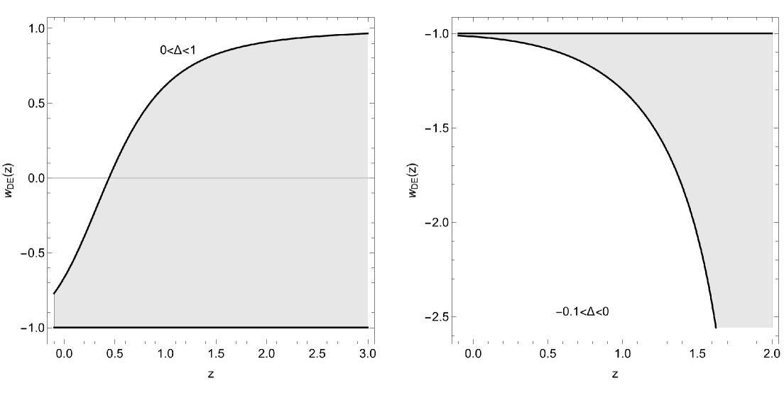
Figure 1: Evolution of the effective dark energy equation-of-state parameter $w_{\mathrm{DE}}(z)$ for different values of the parameter $\Delta$. The left panel corresponds to $\Delta>0$, while the right panel corresponds to $\Delta<0$. We have set $\Omega_{m0}=0.27$. The gray area represent the full set of curves, with boundaries the values of the $\Delta$ at the limits.

For the purposes of studying the late-time evolution of the Universe, we omit the radiation component in Eq. (24), as its effects are negligible. Under this assumption, we can write

$$E(z)\simeq\left[\Omega_{m0}\left(1+z\right)^{3}+\left(1-\Omega_{m0}\right)\right]^{\frac{1}{2-\Delta}}.$$ (25)

In order to understand the equivalent dynamical dark energy model analogue related to Barrow entropy, we write the following Hubble function

$$E_{D}(z)\equiv\left[\Omega_{m0}\left(1\!+\!z\right)^{3}+\left(1\!-\!\Omega_{m0}\right)\exp\left(\!3\int\frac{1\!+\!w_{\mathrm{DE}}\left(z\right)}{1+z}dz\right)\right]^{\frac{1}{2}}\!\!.$$ (26)

Thus, the effective equation-of-state parameter $w_{\mathrm{DE}}\left(z\right)$ can be defined as

$$w_{\mathrm{DE}}\left(z\right)=\frac{\left(1+z\right)^{-3}\Delta\hskip 1.42262pt\Omega_{m0}+\left(1+z\right)^{-6}\left(\Delta-2\right)\left(1-\Omega_{m0}\right)}{\left(2-\Delta\right)\left[\left(1+z\right)^{-3}\left(1-\Omega_{m0}\right)+\Omega_{m0}\right]\left\{\left(1+z\right)^{-3}-\Omega_{m0}\left\{1+\left[\left(1+z\right)^{3}-1\right]\Omega_{m0}\right\}^{\frac{2}{\Delta-2}}\right\}}.$$ (27)

It is straightforward to verify that $w_{\mathrm{DE}}\rightarrow-1$ as $\Delta\rightarrow 0$, thereby recovering the $\Lambda$CDM behavior in the limit where Barrow entropy reduces to the standard area-law scaling.

In Fig. 1 we present the $w_{\mathrm{DE}}(z)$ range for different values of the parameter $\Delta$. As we observe, for $\Delta>0$, we have $w_{\mathrm{DE}}(z)>-1$. On the other hand, phantom behaviour, namely $w_{\mathrm{DE}}(z)<-1$, occurs when $\Delta<0$.

III Observational Constraints

In this section we first describe the data that we use in order to constrain the modified Hubble function, and then we present the results on the scenario of modified cosmology through Barrow entropy.

• Observational Hubble Data (OHD): This data set includes 31 direct measurements of the Hubble parameter from passive elliptic galaxies, known as cosmic chronometers. The measurements for redshifts in the range $0.09\leq z\leq 1.965~$as summarized in Vagnozzi et al. (2021).

• Pantheon+ (SN/SN₀): This set includes 1701 light curves of 1550 spectroscopically confirmed supernova events within the range $10^{-3}<z<2.27~$Brout et al. (2022). The data provides the distance modulus $\mu^{obs}~$at observed redshifts $z$. We consider the Pantheon+ data with the Supernova H0 for the Equation of State of Dark energy Cepheid host distances calibration (SN₀) and without the Cepheid calibration (SN).

• Baryonic acoustic oscillations (BAO): These data are provided by the SDSS Galaxy Consensus, quasars and Lyman-$\alpha$ forests Ross et al. (2020) and the recent data from the DESI DR2 collaboration Abdul Karim et al. (2025).

For the analysis, we employ COBAYA Torrado and Lewis (2019, 2021), with a custom theory and the PolyChord nested sampler Handley et al. (2015a, b) which provides the Bayes evidence. We consider the free parameters to be the energy density of the dark matter $\Omega_{DM}$, the Hubble constant $H_{0}$, the parameter $\Delta$, and the $r_{drag}$ which refers to the maximum distance sound waves could travel in the early Universe before the drag epoch. For the energy density of the baryons we consider the value provided by the Planck 2018 collaboration Aghanim et al. (2020), $\Omega_{b0}=0.0486,$ while the radiation can be omitted since its effects are neglected in the late universe.

We perform our analysis for different datasets. Specifically we consider the datasets $\mathbf{D}_{1}:$SN+BAO, $\mathbf{D}_{2}:$SN+OHD+BAO, $\mathbf{D}_{3}:$SN₀+BAO and $\mathbf{D}_{4}:$SN₀+OHD+BAO.

Barrow entropy is defined for $\Delta>0$. However, BAO data supports a phantom behaviour in the past. Consequently, from Fig. 1 we observe that the effective equation of state parameter has a phantom behaviour in the past for $\Delta<0$. Thus, for $\Delta$ we consider the prior $-0.5<\Delta<0.5$, this prior allow us to compare our results with the previous analysis Anagnostopoulos et al. (2020).

The best fit cosmological parameters for the two different priors are presented in Table 1. Additionally, in Fig. 2 we present the likelihood contours for the best-fit parameters of the scenario for the datasets $\mathbf{D}_{2}$ and $\mathbf{D}_{4}$. As we see, the best fist parameter $\Delta$ is found to be negative, while the zero and the positive values are in the range of $2\sigma$ for the datasets $\mathbf{D}_{1},$ $\mathbf{D}_{2}$, $\mathbf{D}_{3}$ and $1\sigma$ for the dataset $\mathbf{D}_{4}\,$. This is different from the results presented in Anagnostopoulos et al. (2020), where the zero value was within the $1\sigma$. Finally, note that for the $\mathbf{D}_{4}:$SN₀+OHD+BAO dataset, we obtain a value of $H_{0}=72.2_{-0.9}^{+0.9}$, and thus offering an alleviation for the $H_{0}$ tension Di Valentino et al. (2025).

Additionally, in order to compare the fitting efficiency and the behavior of the scenario with that of $\Lambda$CDM paradigm, we fit the latter with the same datasets. In order to compare the two different scenarios, we make use of the Akaike Information Criterion Akaike (1974) (AIC) and the Jeffrey’s scale Jeffreys (1961) for the Bayes evidence $\log Z$. These criteria are used to compare models with different parametric space. Indeed, modified cosmology through Barrow entropy has an additional free parameter.

In Table 2 we present the difference of the statistical parameters between the two models. It follows that the entropic model leads to a $\chi_{\min}^{2}$ which is slightly smaller for the datasets that we investigate. However, from the AIC and Jeffrey’s scale for the $\log\left(\frac{\mathbf{Z}_{\Lambda}}{\mathbf{Z}}\right)$ we infer that there is a Weak/Moderate evidence in favor of the $\Lambda$CDM.

Table 1: Cosmological constraints on modified cosmology through Barrow or Tsallis entropy. The results for Tsallis exponent $\delta$ are obtained from those of $\Delta$ under the identification $\Delta\rightarrow 2(\delta-1)$.

Barrow Entropy	$\mathbf{H}$0	$\mathbf{\Omega}_{m0}$	$\mathbf{\Delta}$
SN+BAO	$69.4_{-5.3}^{+3.9}$	$0.297_{-0.033}^{+0.029}$	$-0.096_{-0.075}^{+0.075}$
SN+OHD+BAO	$68.1_{-1.6}^{+1.6}$	$0.297_{-0.031}^{+0.028}$	$-0.093_{-0.074}^{+0.074}$
SN0+BAO	$73.6_{-0.99}^{+0.99}$	$0.298_{-0.074}^{+0.074}$	$-0.095_{-0.074}^{+0.074}$
SN0+OHD+BAO	$72.2_{-0.9}^{+0.9}$	$0.280_{-0.031}^{+0.028}$	$-0.066_{-0.077}^{+0.077}$

Table 2: Comparison of Barrow Entropy with the $\Lambda$CDM paradigm.

Barrow Entropy	$\mathbf{\chi}_{\min}^{2}-\mathbf{\chi}_{\Lambda\min}^{2}$	$\mathbf{AIC}-\mathbf{AIC}_{\Lambda}$	$\log\left(\frac{\mathbf{Z}_{\Lambda}}{\mathbf{Z}}\right){\,}$
SN+BAO	$-0.4$	$+1.6$	$+0.65$
SN+OHD+BAO	$-0.5$	$+1.5$	$+1.04$
SN0+BAO	$-0.6$	$+1.4$	$+0.85$
SN0+OHD+BAO	$+0.5$	$+2.5$	$+1.57$

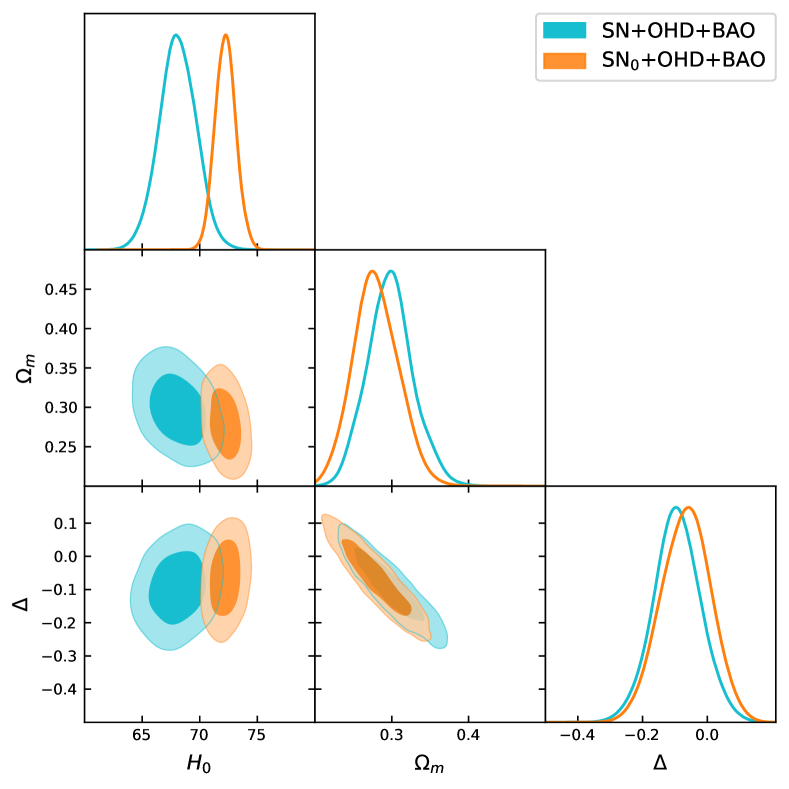
Figure 2: Likelihood contours for the best-fit parametersof modified cosmology through Barrow entropy, for the datasets $\mathbf{D}_{2}:$SN+OHD+BAO, and $\mathbf{D}_{4}:$SN₀+OHD+BAO. The results for Tsallis exponent $\delta$ are obtained from those of $\Delta$ under the identification $\Delta\rightarrow 2(\delta-1)$.

IV Conclusions and Outlook

A well-established conjecture in theoretical physics suggests a deep connection between gravity and thermodynamics. Within cosmological contexts, this correspondence implies that the standard Friedmann equations governing the Universe expansion may be derived from the first law of thermodynamics using the standard Bekenstein-Hawking entropy. On the other hand, Barrow entropy is an one-parameter modification of Bekenstein-Hawking entropy, arising from quantum-gravitational effects that induce a fractal structure on the surface of black holes. Similarly, Tasllis entropy is an one-parameter modification arising within the framework of nonextensive statistical mechanics. Hence, if one applies the gravity-thermodynamics conjecture, but using the modified Barrow or Tsallis entropy then one obtains modified Friedmann equations and thus a modified cosmological scenario.

In this work we use observational data from Supernova Type Ia (SNIa), Cosmic Chronometers (CC), and Baryonic acoustic oscillations (BAO), including the recently released DESI DR2 data, in order to extract constraints on the scenario of modified cosmology through Barrow and Tsallis entropy. Firstly, we examined the behavior of the effective dark-energy equation-of-state parameter according to the values of the Barrow exponent $\Delta$, or the Tsallis exponent $\delta=1+\Delta/2$, showing that it lies in the quintessence regime for positive $\Delta$, while it lies in the phantom regime for negative $\Delta$. Then we performed the full observational confrontation, focusing on the constraints on $\Delta$, on the current matter density parameter $\mathbf{\Omega}_{m0}$ and on the current Hubble function value $H_{0}$.

As we showed, the best-fit value for $\Delta$ is found to be negative, while the zero value, which corresponds to $\Lambda$CDM paradigm, is allowed only in the range of $2\sigma$ for the datasets $\mathbf{D}_{1}:$SN+BAO, $\mathbf{D}_{2}:$SN+OHD+BAO, $\mathbf{D}_{3}:$SN₀+BAO and in the range of $1\sigma$ for the dataset $\mathbf{D}_{4}\,$. Additionally, for the case of the $\mathbf{D}_{4}:$SN₀+OHD+BAO dataset, we obtained a value of $H_{0}=72.2_{-0.9}^{+0.9}$, which offers an alleviation for the $H_{0}$ tension. Finally, by applying information criteria such as the Akaike Information Criterion and the Bayes evidence, we compared the fitting efficiency of the scenario at hand with $\Lambda$CDM cosmology, showing that the latter is slightly favoured.

Recent observational datasets from DESI DR2 collaboration seem to favour dynamical dark energy. Hence, it is crucial to investigate scenarios that deviate from $\Lambda$CDM paradigm in a dynamical way. Modified cosmologies through Barrow, Tsallis and other extended entropies lie in this category of dynamical dark energy. Thus, they may offer an alternative for the description of nature.