Creating non-reversible rejection-free samplers by rebalancing skew-balanced Markov jump processes
Abstract
Markov chain sampling methods form the backbone of modern computational statistics. However, many popular methods are prone to random walk behavior, i.e., diffusion-like exploration of the sample space, leading to slow mixing that requires intricate tuning to alleviate. Non-reversible samplers can resolve some of these issues. We introduce a device that turns jump processes that satisfy a skew-detailed balance condition for a reference measure into a process that samples a target measure that is absolutely continuous with respect to the reference measure. The resulting sampler is rejection-free, non-reversible, and continuous-time. As an example, we apply the device to Hamiltonian dynamics discretized by the leapfrog integrator, resulting in a rejection-free non-reversible continuous-time version of Hamiltonian Monte Carlo (HMC). We prove the geometric ergodicity of the resulting sampler under certain convexity conditions, and demonstrate its qualitatively different behavior to HMC through numerical examples.
keywords:
[class=MSC]keywords:
, and
1 Introduction
Markov Monte Carlo methods enable sampling from a distribution specified by an unnormalized probability density, for example a posterior distribution in Bayesian inference. The most common device used to construct such samplers is Metropolization [28, 19], the introduction of an accept/reject step in the process to enforce a detailed balance condition with respect to the target distribution. However, the resulting reversibility of the sampler can introduce random walk behavior leading to slow mixing, requiring careful tuning of sampler hyperparameters [30, 2]. This is a driving motivation behind the recent interest in non-reversible Monte Carlo methods that potentially overcome these drawbacks, see e.g. [31, 26, 2].
Our main contributions in this paper are:
-
1.
We introduce a rebalancing device that turns a continuous-time jump process that satisfies a skew-detailed balance condition for a reference measure into a sampler for a target measure that is absolutely continuous with respect to the reference measure. The resulting samplers are rejection-free, non-reversible, and continuous-time.
-
2.
We use the device on a simple example, the leapfrog integrator, to create a rejection-free non-reversible continuous-time version of Hamiltonian Monte Carlo (HMC). We prove the geometric ergodicity of the resulting sampler under certain conditions on the target distribution.
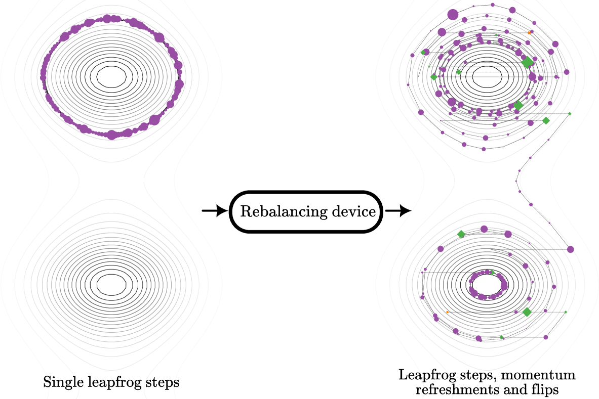
The idea of the rebalancing device is illustrated in Fig. 1: turning a simple jump process consisting of only leapfrog discretized Hamiltonian dynamics, with unit rate exponential waiting times, into a sampler that samples a desired target distribution by altering the jump rates and adding a flip transition that changes the sign of the momentum. Adding a momentum refreshment to the process is necessary for ergodicity. While ostensibly based on the same properties as HMC, it behaves qualitatively different. The essential difference of the proposed sampler is that it avoids random walk behavior that may be present in HMC [30]. This is due to its non-reversibility, which manifests as robustness to tuning and mixing for a wider range of hyperparameters. In practice, the computational cost in gradient evaluations is comparable to HMC, and cheaper than other popular non-reversible samplers based on Poisson thinning [3].
1.1 Related work
The main principle underlying the proposed mechanism of continuous-time rebalancing is skew-detailed balance. Based on this principle, a general framework for discrete-time non-reversible Markov chain samplers with rejections is laid out in [2] with a detailed review of instances in the literature, e.g. [1, 17, 20, 35, 15, 36]. In contrast, our continuous-time method constructed via Markov jump processes is rejection-free, and directly allows for a stochastic jump kernel. A similar approach, which uses the same skew-detailed balance conditions as our paper, has also been taken in [31] but in a discrete state space setting (see also [21] for spin models and [34] for momentum accelerated sampling on graphs). Another approach to obtain a rejection-free non-reversible continuous-time sampler is based on piecewise deterministic Markov processes, see e.g. [2, 3, 10, 5, 6]. Other continuous-time versions of HMC than our example have been proposed, in particular [8]. Subsequent to the first availability of our work, the formalism of the class of Markov jump processes under study in this paper was greatly improved in the reversible case by [25], and our work provides a motivation for study of the non-reversible case.
1.2 Structure of the paper
In Section 2, we first introduce the necessary notation and definitions for Markov jump processes and the skew-detailed balance condition. Then, we describe the rebalancing device and prove the main theorem of the paper, which states that the construction in fact results in a jump process with the intended stationary measure. In Section 3, we apply the device to the leapfrog integrator to obtain a sampler, and prove its geometric ergodicity under certain conditions on the target distribution. We present its implementation and how practical estimation is carried out. In Section 4, experiments to demonstrate the behavior of the sampler are presented. Finally, Section 5 concludes the paper with a discussion of research directions and generalizations.
2 Rebalancing of skew-balanced Markov jump processes
In this section, we introduce the concept of a skew-detailed balance condition for a Markov jump process and show how to construct a new Markov jump process that samples a target measure that is absolutely continuous with respect to the reference measure. First, we introduce the necessary notation and definitions.
2.1 Markov jump processes
Following [22], let the state space be a locally compact Hausdorff space with countable base. Denote by the Borel -algebra on . A Markov jump process on is a continuous time stochastic process on with almost surely right-continuous paths that are constant except for a countable number of jump times. Note that we only consider time-homogeneous processes, where for all . We denote the jump times by . The law of the process is determined by:
-
1.
The initial distribution on .
-
2.
The rate function . Conditional on , the time until the next jump is exponentially distributed with rate .
-
3.
The jump kernel , such that for all .
This entails by the Markov property that form an independent sequence of random variables and an embedded discrete-time Markov chain with transition kernel . We also define the rate kernel as the specific rate of jumps from to . Both the total rate and the jump kernel are determined through and , Finally, for bounded the generator of the process is defined [22, Proposition 19.2] as the operator acting on a bounded measurable function by
| (2.1) |
2.2 Skew-detailed balance and rebalancing
We now describe the device that turns a jump process into a sampler. The key idea is a skew-detailed balance condition for the jump process [2, 31]. A Markov jump process with rate kernel is in skew-detailed balance with respect to a transformation and a measure if
| (2.2) |
for all integrable .
To use the device to create a sampler for a probability measure on , one requires three ingredients:
-
1.
A reference measure on such that , i.e., is absolutely continuous with respect to .
-
2.
An involution , that is, a map satisfying , which is isometric under both and , i.e., and for all .
-
3.
A rate kernel that is in skew-detailed balance with respect to and .
These suffice to obtain a sampler targeting the right measure, as shown by the main theorem in this section:
Theorem 2.1.
Let be a probability measure on that is dominated by a -finite reference measure , , and let be an isometric involution for both. Assume there is a rate kernel with bounded rate such that skew-detailed balance (2.2) holds for under and . Let
| (2.3) |
where is a bounded function that satisfies the balancing condition,
| (2.4) |
We define
| (2.5) |
where
Then is the stationary measure of the jump process with rate kernel .
Examples of bounded balancing functions include, but are not limited to, the Metropolis balancing function or the Barker balancing function [38, 25]. It is a classical result that all such balancing functions satisfy up to time scaling factors [2], making a natural default choice to encourage movement. It would be of interest to consider unbounded balancing functions such as , which have been promising in some settings [39], but we omit them here in the interest of simplifying the existence theory. Finally, the trivial involution always satisfies the hypotheses, but will instead produce a reversible process as (2.2) reduces to detailed balance.
The first step of proving Theorem 2.1 is to state conditions for stationarity or invariance. Recall that a Markov process has a stationary measure if
| (2.6) |
where . Under our assumptions, the skew-detailed balance condition together with an additional semi-local condition yields the necessary stationarity.
Proposition 2.2.
Let be a probability measure, a -isometric involution , and a rate kernel with bounded rate . If a (weaker) skew balance condition
| (2.7) |
holds for all integrable , and the semi-local condition
| (2.8) |
holds with respect to and , then is the stationary measure of the jump process with rate kernel .
Proof.
By a standard theorem [14, Proposition 9.2], it suffices to verify that
for all bounded measurable test functions to obtain the conclusion.
Recall the transformation formula for a bijection :
The proposition follows by splitting the integral over the difference (as , , and are bounded) and showing that the first term equals the second. Using (2.7) and the definition of the rate
and using (2.8) to substitute we obtain
where we applied the transformation formula using that is a bijection. Now, as is -isometric, we have
This cancels the second term, and we have established (2.7) for any bounded measurable test function . ∎
The preceding proposition motivates the choice of in Theorem 2.1 as the minimal solution to the semi-local condition (2.8), similar to the choice in [31]. Any solution will yield invariance by the proposition, but a non-minimal one will induce additional jumps with which are not necessary to maintain invariance. The minimal choice ensures only one of and is nonzero, so that the process is truly non-reversible and rejection-free.
We also require the following lemma:
Lemma 2.3.
If and is isometric for both, then -almost everywhere
| (2.9) |
Proof.
The calculation
shows that is almost everywhere a Radon–Nikodym derivative of with respect to . ∎
We are now ready to prove Theorem 2.1.
Proof of Theorem 2.1.
Since is a bounded function, it follows that is a rate kernel with bounded rate , and thus by Proposition 2.2 it suffices to verify (2.7) and (2.8) to establish stationarity.
The choice of ensures that (2.8) is satisfied by construction. To see this, take without loss of generality with (otherwise simply apply ). It follows that and we deduce
A way to construct an appropriate rate kernel is to use a -isometric deterministic bijective map that is skew-symmetric with respect to , in the sense that
| (2.10) |
as shown by the following proposition:
Proposition 2.4.
Let be a measure and a -isometric involution. Suppose is -isometric, bijective, and satisfies (2.10). Let be a bounded rate function which is invariant under and , and define
where is the Dirac measure at . Then the rate kernel is in skew-detailed balance with respect to and .
Proof.
For any -integrable , a direct calculation with the change of variables yields
as required. ∎
3 A sampler based on Hamiltonian dynamics
There are several Markov Monte Carlo methods that use techniques from the integration of Hamiltonian dynamics to obtain samples from a target distribution , where . A common idea behind such samplers is to augment the state space with a momentum variable and to consider the dynamics governed by the Hamiltonian and is the kinetic energy. These dynamics are described by Hamilton’s equations, which in this case are given by
| (3.1) | ||||
The motion induced by these equations are used to construct Markov processes that are stationary for the measure . The measure admits the desired target measure as a marginal, allowing the estimation of expectations from trajectories of the Markov process.
The function is constant along solutions to Hamilton’s equations (3.1). Furthermore, the dynamics are reversible by changing the sign of the momentum coordinate, meaning that if we follow the dynamics for a certain amount of time, then turn around and move backwards in time for just as long, we end up where we started. Hamiltonian dynamics also have the property that the phase space volume is preserved, meaning that the volume of a subset of the phase space remains constant under the dynamics. This is known as Liouville’s theorem and follows since the determinant of the Jacobian of the transformation is unity.
However, unless and are particularly simple, it is not possible to solve Hamilton’s equations exactly. Thus, one typically resorts to numerical integration schemes to approximate the solution of (3.1). The numerical method should preserve the key properties of the Hamiltonian dynamics, in our case reversibility and phase space volume. Off-the-shelf integrators typically do not have these properties, so we must resort to symplectic integrators. The canonical choice is the leapfrog integrator, which is a second-order method that alternates between updating the momentum and the position variables. The leapfrog integrator discretizes the Hamiltonian dynamics by
| (3.2) | ||||
We use the notation to denote the mapping from to given by the leapfrog method (3.2). For more details on Hamiltonian dynamics, the leapfrog methods and symplectic integration in general, see for instance [18, 23, 9].
3.1 Sampler construction
Equipped with the machinery of Theorems 2.1 and 2.4, we can now construct a sampler based on the leapfrog integrator. We begin by describing the construction of the process that is re-balanced to give rise to the sampler. We set . The process can only perform one move: jump by taking a leapfrog step according to the Hamiltonian , where is proportional to the target density and is the kinetic energy of a unit mass particle. The process waits an -distributed time before taking a leapfrog step. Thus, in the context of Section 2.2, , and .
This process obviously does not sample from the measure , where denotes the Lebesgue measure. However, note that is preserved under by the volume preservation. Therefore, since , we can apply Theorem 2.1 to construct a sampler that samples from as long as we specify an appropriate involution. Our choice is to add sign-flips of the momentum variable, i.e., we let
| (3.3) |
Note that . Furthermore,
| (3.4) |
Thus, we can apply the device provided by Theorem 2.1 to obtain a re-balanced process that can take two different types of steps: leapfrog steps and sign-flips of the momentum variable. We select as the balancing function. Since the Radon–Nikodym derivative of with respect to is
Theorem 2.1 gives that the rate of the leapfrog arrival is
and that the rate of the sign-flip arrival is
The rate kernel is
The continuous time Markov process is controlled by just one tuning parameter, the leapfrog integrator step size . While has as a stationary distribution, it is, in general, not ergodic. For this reason, we introduce a momentum refreshment mechanism that is independent of the dynamics, as we can sample directly from the corresponding marginal . The refreshments arrive independently at the rate . This adds the term to the rate kernel.
Thus, there are now three steps that can take: leapfrog, sign-flip, and refresh steps. Therefore, we name the process the Flip-Frog-Fresh (FFF) sampler. The final definition is as follows: if , the process stays in for an independent random time , where , then it jumps to
where is an independent momentum refreshment.
The generator of the process is thus, by (2.1), the operator defined by
| (3.5) | ||||
which simplifies to
Consequently, we split the generator into three terms, where
| (3.6) | ||||
The FFF sampler preserves the target measure by construction:
Proposition 3.1.
The measure is invariant for the Markov process .
Proof.
The proposition follows directly from Theorems 2.1 and 2.4 as the hypotheses have been verified above. ∎
We remark that the generator (3.5) resembles that of a numerical version of Randomized HMC [8, Eq. 36], because the latter is (up to time scaling) a Metropolized version of the leapfrog jump process with . This construction is also invariant by Proposition 2.2 since the Metropolized rates satisfy the semi-local condition (2.8). However, they are not the minimal rates and will introduce more flips than necessary, so that the resulting process is reversible and not rejection-free in the sense discussed below.
3.2 Comparison to HMC
The properties of the leapfrog dynamics that the construction of the FFF sampler relies on, reversibility and volume preservation, are the same properties underpinning HMC. It is remarkable that, by simply applying them differently, one can instead obtain a rejection-free, non-reversible, and continuous-time sampler.
In the construction of HMC, the basis is detailed balance. By observing that the leapfrog integrator composed with a flip is an involution thanks to the reversibility, it follows by volume preservation of and that detailed balance holds for the Lebesgue measure. However, this kernel alone does not preserve the target measure, as only approximates the Hamiltonian dynamics. To remedy this, a Metropolis–Hastings correction is applied, where the volume preservation in particular facilities the computations in the acceptance probability. Finally, the process is made ergodic by adding momentum refreshments.
The FFF sampler, however, relies on skew-detailed balance. Again, the volume preservation of ensures that the Lebesgue measure is preserved, but as detailed in Section 3.1 the reversibility is instead interpreted as skew-symmetry (3.4) with respect to . This allows the application of the rebalancing device, adding flips according to to preserve the target measure. Finally, just as for HMC, ergodicity necessitates the addition of a momentum refreshment.
That the FFF sampler is rejection-free implies that staying for a long duration in a point due to high target probability is essentially free as we directly simulate the waiting time. The effect of this is most pronounced if the target has a narrow ridge, or when starting in the mode of the target. For example, under the assumption of independent target components, to keep the error in the Hamiltonian (and thus or the acceptance probability) constant as the dimension increases, the step size must decrease as [30]. This does not inhibit FFF from leaving the state at a constant cost as long as the refreshment rate is small enough. However, when HMC is stuck, it will continue to generate proposals until one is accepted, each proposal requiring a new evaluation of the Hamiltonian. Thus, in high dimensions, avoiding random-walk behavior also requires leapfrog steps, a polynomially increasing computational cost.
3.3 Geometric ergodicity
We now establish the geometric ergodicity of the proposed sampler for a class of potentials , using the Meyn–Tweedie approach [29] as formulated in [32]; this formulation allows a particularly straightforward proof. The Meyn–Tweedie approach has also been used for HMC in e.g. [13, 24]. Geometric ergodicity shows not only that refreshments are enough for convergence of the ergodic averages, but also, thanks to the exponentially fast convergence, entails a corresponding central limit theorem.
Assumption 1.
The potential satisfies the tail condition that is convex for some and . Furthermore, is a Lipschitz function with Lipschitz constant .
This assumption is comparable to e.g. those of [12]. The proof is divided into two parts. First, we prove a drift condition, i.e., that there is a suitable Lyapunov function for which there are constants and such that
| (3.7) |
Then, we prove a minorization condition, meaning that there exists a probability measure on , a time , and a constant such that
| (3.8) |
where for some . In our case, we have that both the drift and minorization conditions hold, as detailed in the following theorem:
Theorem 3.2.
Let Assumption 1 hold. Furthermore, let the leapfrog integration step size satisfy the bound
| (3.9) |
Then, the norm-like function
| (3.10) |
where is such that , satisfies (3.7) for some and . Furthermore, (3.8) is satisfied for some , and as above. It follows that the process is geometrically ergodic (see [32] for a definition).
The proof is postponed to Appendix A. We note that it relies on balancing leapfrog jumps with refreshments, and does not use any property of the flips other than the boundedness of . In particular, the proof also applies to the aforementioned numerical version of Randomized HMC, and answers a conjecture about its geometric ergodicity posed in [8, Section 6.2]. Hence, non-reversibility does not change the qualitative convergence behavior, but it is possible that there is a quantitative difference which this approach cannot capture.
3.4 Extensions
We now enumerate some extensions of the FFF sampler that can be useful in practical problems.
-
1.
Mass matrices. The marginal of the momentum variable, from which the refreshments are drawn, was chosen as a standard Gaussian distribution. This is not the only choice preserved by . Indeed, it is common in HMC to instead use the distribution , where is a symmetric positive definite mass matrix, in particular when the target distribution is not isotropic and a common step size is inefficient. The modification is immediate, as it only corresponds to a linear change of variables on , and as noted by [30], setting and we are back to the original setting with no mass matrix.
-
2.
Multiple leapfrog steps. Taking multiple leapfrog steps is a straightforward modification. We apply the device to the process with a deterministic jump kernel that takes leapfrog steps after an exponential waiting time, and obtain a process with rates appropriately modified, i.e., the rate of leapfrog jumps becomes
and rate of the sign-flip arrival becomes
-
3.
Partial momentum refreshments. A variant of refreshment that is sometimes used for HMC is partial momentum refreshment [20, 30], i.e., correlating the new momentum with the previous as , where is the new independently sampled momentum and is the correlation hyperparameter. The target stationary distribution of the process remains unchanged. For HMC, this could reduce random walk behavior similarly to FFF, but requires introducing an extra flip upon rejection to preserve invariance. In FFF this additional flip is not necessary.
3.5 Estimator and implementation
Having established ergodicity we deduce, as previously mentioned, convergence of the sample averages to the desired expectation. However, for a continuous-time Markov jump process, we obtain an immediate variance reduction if the waiting times are replaced by their expectations. This is the estimator which we use in practice, and also implies that the actual jump times are not necessary in the implementation, just the rates at each state.
Proposition 3.3.
If the process is ergodic, it holds for any -integrable function that
almost surely, for almost every , where .
Proof.
A direct application of the ergodic theorem and the Rao–Blackwell theorem as the total rate is bounded from above and below, see [11, 39]. The geometric ergodicity proven in Theorem 3.2 implies a stronger version of the above proposition where the convergence holds for every [33]. ∎
Furthermore, by reusing previous computations, one can achieve efficiency improvements in the sampler which are important to make the computational cost comparable to that of HMC. Every simulated jump of the process first requires computing the rates, which in turn requires evaluating in the current state, after a forward step (), and after a backward step (). Each such step requires one evaluation of assuming the implementation carries forward in the current state as is commonly done when implementing HMC. (If we generalize to leapfrog steps, the cost scales accordingly by .) However, if the implementation remembers the forward and backward states, then
-
•
a leapfrog step only requires one forward evaluation of because the value in the current state becomes the new backward value,
-
•
a flip step is free because the forward and backward values of are simply swapped,
-
•
but a refreshment step still requires two new evaluations of , forward and backward.
This suggests the heuristic that the frequency of refreshments should be roughly that of flips, as returning along the same path does not contribute information to the sample, while also balancing out the cost of exploration. The result is that every simulated jump on average requires close to one evaluation of , which is the cost of HMC, and only in the worst case, two evaluations. In practice, this is much cheaper than non-reversible samplers based on Poisson thinning and piecewise deterministic Markov processes [3], such as the Zig-Zag sampler [5] or the Bouncy Particle sampler [10], while comparable to the cost of other non-reversible gradient-informed samplers such as the Hug-and-Hop sampler [26].
We provide a Julia [4] package implementing the sampler, FFFSampler.jl111Code available at https://github.com/rubenseyer/FFFSampler.jl, which is compatible with the existing Julia ecosystem of statistical packages, in particular AbstractMCMC.jl and Turing.jl. Our code is therefore a drop-in replacement for practitioners working in this framework.
4 Experiments
To evaluate the performance of the FFF sampler, we conduct a series of experiments on various benchmark problems. These experiments are designed to contrast the FFF sampler against HMC.
In all experiments, the performance metric is based on distributional distances. In particular, we use the Kolmogorov–Smirnov (KS) distance
where is the cumulative distribution function of the statistic of interest, and is the empirical cumulative distribution function of the generated sample. The distance is straightforward to compute, as for a jump process trajectory is just a weighted sum over the embedded chain states where the weights correspond to the expected proportion of time spent in the state. In the experiments below we directly use the marginals as statistics, and average the resulting KS distances across several repeated runs. We then report the maximal (i.e., worst) mean KS distance across all marginals.
Our metric differs from the popular choice of metrics within Markov chain Monte Carlo based on effective sample size (ESS), which compare (an estimate of) the asymptotic variance to the corresponding estimator for an i.i.d. sequence [37]. While ESS-based metrics are suitable in the discrete case as they are easily interpretable and can be efficiently estimated, they are less developed in the continuous case, and in particular, it is difficult to normalize them for comparison between the continuous trajectories of FFF and the discrete trajectories of HMC. In contrast, the distributional distances are directly comparable when controlling for a fixed computational budget, which we measure in terms of the number of evaluations of by the algorithm.
For a fair comparison, we do not tune the samplers using heuristics, but instead by a simple grid search over hyperparameters: step size and number of steps for HMC, and step size , number of steps and refreshment rate for FFF. The performance of the samplers is evaluated using the KS distance statistic. Unless otherwise mentioned, we use a fixed computational budget of evaluations of with replicates of each parameter configuration. When we do not have access to the true cumulative distribution function in closed form for the computation of the KS distance, we use million exact samples to approximate it empirically.
4.1 Gaussian target
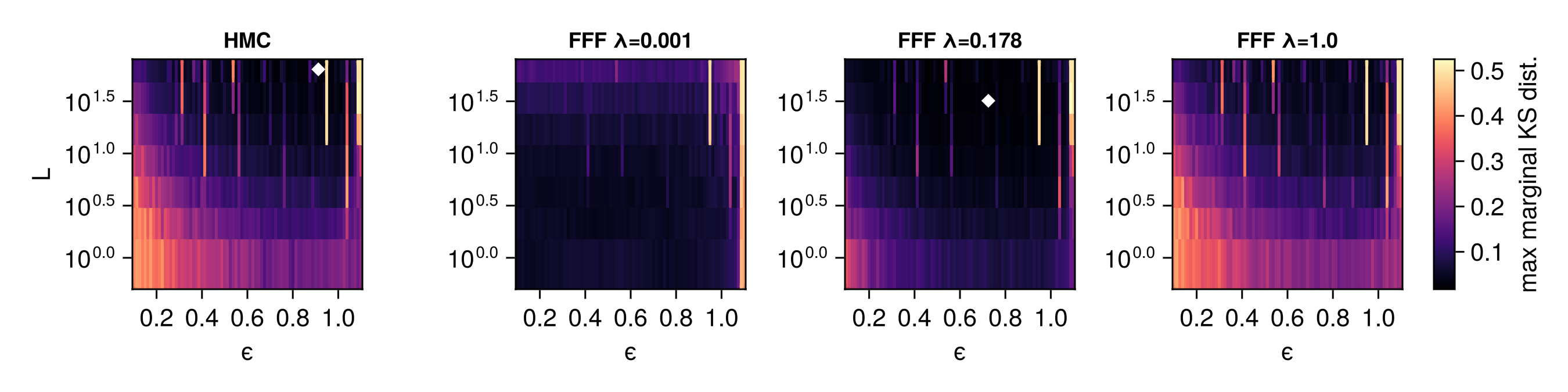
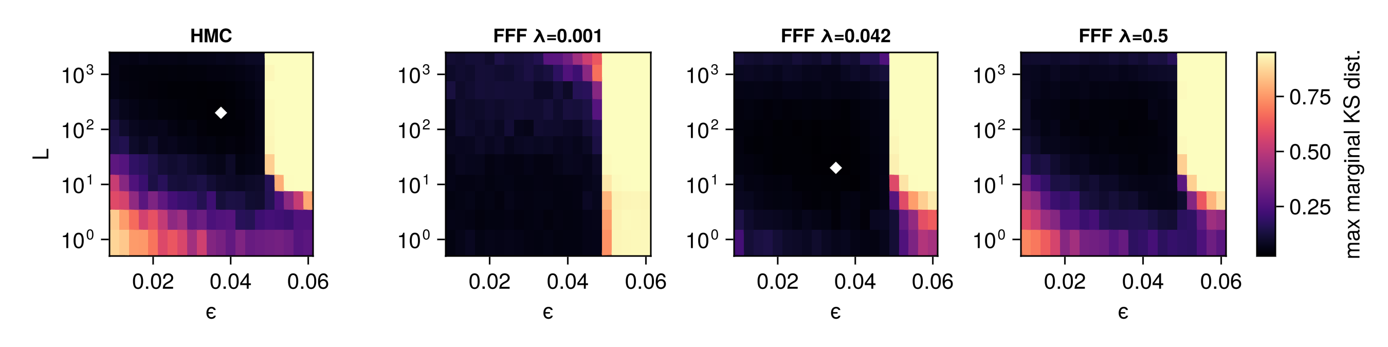
We target a six-dimensional Gaussian distribution with independent components. The mean is set to zero, and the covariance matrix is given by the diagonal matrix
where is the real root of the polynomial . The choice is intended to exacerbate the periodicity issues in Hamiltonian dynamics [30] by yielding many non-overlapping problematic combinations of step size and number of steps . HMC, without estimating an appropriate mass matrix, cannot avoid these issues by using smaller step sizes, as it would cause random walk behavior in the large-scale component. In contrast, the FFF sampler allows a larger range of parameters, as smaller step sizes with lower refresh rates also lead to mixing through keeping the momentum.
The results of the grid search are shown in Fig. 2, where we observe that the FFF sampler indeed has a larger range of parameters that yield acceptable performance than HMC (in fact, FFF marginally beats HMC in the best configuration, taking both fewer and shorter steps).
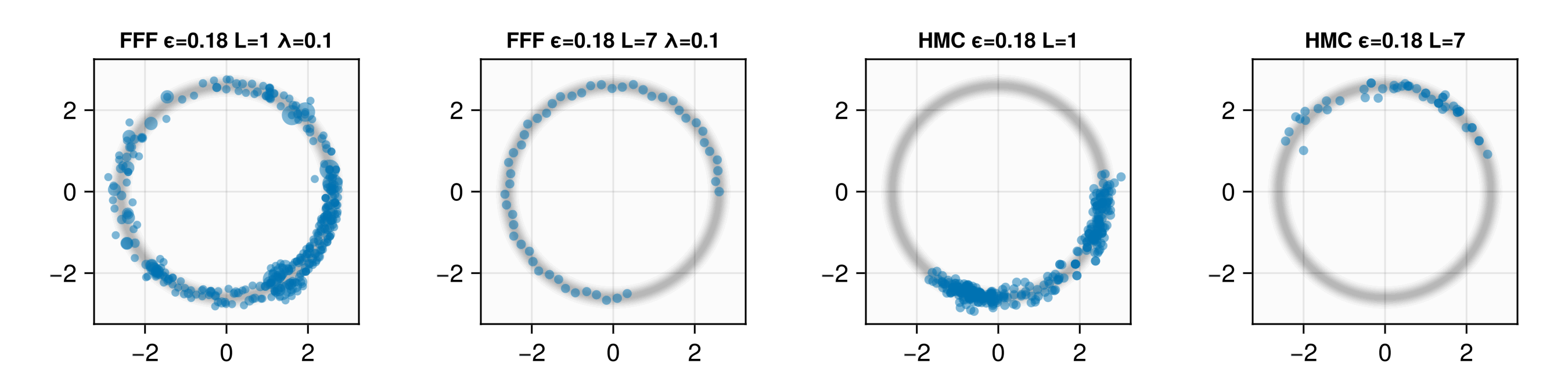
4.2 Donut target
We consider a simple example of a “donut” density to illustrate the non-reversibility of the FFF sampler. HMC, although reversible by construction, is sometimes said to display “non-reversible characteristics” because of the inclusion of the momentum variable. However, obtaining effectively uncorrelated draws may require many small steps. This implies that exploration can be performed much more efficiently in such settings using the true non-reversibility of the FFF sampler.
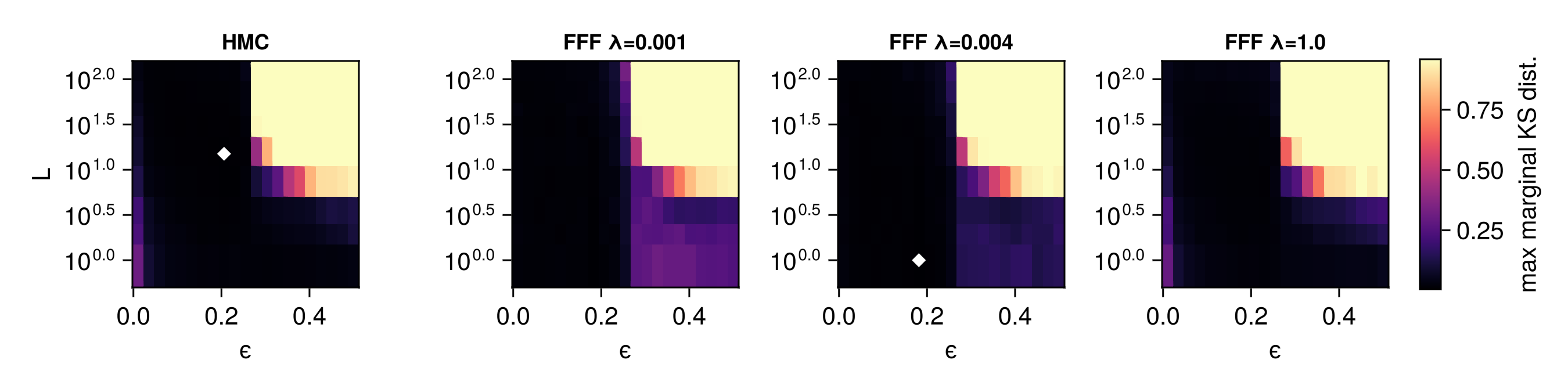
We define the target potential , and run the example in two dimensions with . Short sample trajectories for different settings of FFF and HMC are shown in Fig. 3; note that the two samplers behave drastically different from each other. The random walk behavior of HMC greatly slows the exploration of the state space, a phenomenon that FFF avoids. The results of the grid search are shown in Fig. 4. On such a simple target there is little difference asymptotically as soon as the algorithms are well-tuned, but we see that even small integration times do not inhibit mixing for FFF. Thus, at the same computational cost, we can obtain a denser set of more correlated samples instead of than a sparse set of less correlated samples.
4.3 Banana target
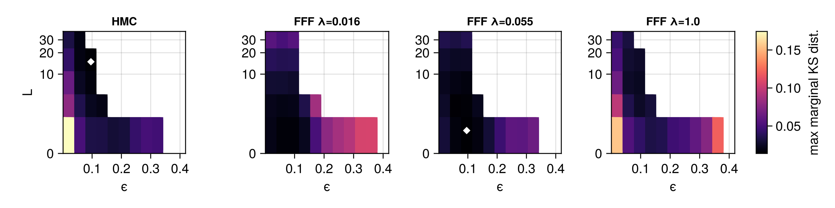
We postulate that ergodicity holds under more general conditions than in Theorem 3.2. Supporting this, we perform an experiment targeting a distribution that does not satisfy the conditions of Assumption 1, the classical challenging “banana” potential [16].
The results of the grid search, with initial state in the right tail, are shown in Fig. 5. Not only do both samplers yield satisfactory results, suggesting that ergodicity holds, but the strengths of FFF are once again highlighted. The Banana target consists of a narrow ridge with differing scales and heavy tails, and thus non-reversibility assists exploration when using small step sizes. In particular, the optimal FFF configuration reduces the number of leapfrog steps by an order of magnitude, once again providing a denser set of samples.
4.4 Bayesian PKPD model
The preceding examples were all synthetic in nature. However, the features exhibited in them can and do occur in actual statistical analysis. As a case study, we consider a benchmark model in PosteriorDB [27], one_comp_mm_elim_abs, representing a one-compartment pharmacokinetic model:
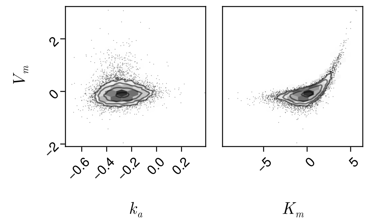
where is the true concentration (mg/l), is the measured concentration (mg/l), is the dosing rate per day, is the Michaelis–Menten constant (mg/l), is the maximum elimination rate per day, is the total dosage (mg), and is the compartment volume (l). The data consists of a series of measured concentrations at fixed times together with and .
This model based on an ODE has comparatively expensive likelihood evaluations requiring the solution of the system, making it desirable that the number of leapfrog steps are kept low for performance. Moreover, the constrained parameter space yields non-linear contours in several posterior marginals of pairs as shown in Fig. 6. The model thus shares several features with the previously covered synthetic models.
The results of the grid search are shown in Fig. 7, where a budget of 150 000 evaluations of was used for performance reasons, and the reference in the distributional distance is chosen as the empirical CDF of the reference samples in PosteriorDB. The underlying ODE solver appears to constrain the Hamiltonian integration time , yielding a narrow range of acceptable hyperparameters. We see that FFF suppresses random walks at small step sizes similar to the Donut and Banana target experiment, and has comparable performance to HMC at . This highlights both the practical interest of the sampler construction and the ease of use with existing software.
5 Conclusion and outlook
We introduce a rebalancing device that, using underlying symmetries in a Markov jump process, constructs samplers which are rejection-free, non-reversible and continuous-time. We demonstrate the device by constructing the FFF sampler based on the leapfrog integrator. Although relying on the same properties of the leapfrog dynamics as HMC, the FFF sampler has several important qualitative differences that follow from the three aforementioned properties. Non-reversibility is often presented as an opportunity for faster convergence, but it is difficult to significantly outperform well-tuned reversible methods that produce effectively uncorrelated samples. Nevertheless, as highlighted in the numerical experiments, though the performance is similar with ideal tuning, the benefit of non-reversibility can still be seen through more robust behavior. In particular, it allows for mixing using very few leapfrog steps even when the step size is small. This means that in settings where the gradient evaluations are expensive, such as in Section 4.4, the FFF sampler is an attractive alternative to HMC as each individual step costs less. The fact that FFF is continuous-time and rejection-free also allows becoming unstuck at virtually no computational cost.
The device presented in this paper is not limited to Hamiltonian dynamics. We end the paper by providing a few examples of how the rebalancing device can be used in other settings.
- 1.
-
2.
Let and . Let be the product Lebesgue measure on , and the kernel corresponding to the deterministic skew-symmetric isometric map
Then and are in skew-detailed balance for the -isometric involution by Proposition 2.4. Given a target measure of the same type as in FFF, we can then apply the rebalancing device and Theorem 2.1 to obtain a sampler, adding refreshments for ergodicity. This construction could be understood as a continuous-time and rejection-free version of [17], with non-reversibility manifesting as the conservation of momentum on lines in . Of course, being less sophisticated compared to FFF, more flips will occur, and hence one explores less efficiently than with Hamiltonian dynamics.
-
3.
The above construction also works on discrete spaces, for example with as the counting measure. Refreshments can be avoided in this case. More generally, by applying the rebalancing device to discrete spaces with graphical structure and a Zanella process, one can recover constructions in [31].
-
4.
The rebalancing device also applies to non-deterministic jump kernels. For instance, one way to avoid the periodicity issues in Section 4.1 is to introduce stochasticity in the step size [30] or integration time [8]. In the setting of Section 3, write to highlight the dependence of the leapfrog map on the step size , and let be a probability distribution on positive step sizes. Then the rate kernel
is in skew-detailed balance with respect to and , by a simple application of Fubini’s theorem and the skew-detailed balance for the leapfrog kernel. One can then proceed with rebalancing to obtain the analogous sampler to the FFF sampler.
-
5.
Let denote the space of directed graphs with vertices. Let us write or for if is obtained from by inserting a single directed edge or equivalently if is obtained from by deleting one.
The uniform distribution over is in skew-detailed balance with the rate kernel on
and the -isometric involution . Note that is not deterministic in this example. From here we can use Theorem 2.1 to construct samplers for any distribution absolutely continuous with respect to . By compactness of , geometric ergodicity follows for a target for which the FFF sampler is irreducible. For example, this holds for the uniform distribution on the space of directed acyclic graphs (DAGs). Similarly, [34] extends the idea to Markov equivalence classes of DAGs, where a special case of Theorem 2.1 is established by [34, Lemmas 1–2].
Appendix A Proof of geometric ergodicity
As mentioned previously, the proof of geometric ergodicity is done in two main parts: the drift condition, and the minorization condition. We then connect these two together to establish the result.
A.1 Drift condition
Our proof of the drift condition requires two lemmas. We first give a sufficiently fine-grained Taylor expansion of the terms for how the Hamiltonian changes for a forward step.
Lemma A.1.
Let be twice continuously differentiable and . Then with ,
| (A.1) |
where and .
Proof.
We have
Using Taylor’s formula, we get
| (A.2) |
Expanding leads to
Next, we require control of the remainder in our expansion.
Lemma A.2.
Let Assumption 1 hold. Then, in the setting of the preceding Lemma A.1, there exists a such that
where .
Proof.
By assumption, the function is convex outside a ball with radius . Let denote the smallest (possibly negative) eigenvalue of inside this ball.
With , we expand
where we have substituted , so that instead of integrating along a line of length , we integrate along a line of length . In this case, only the part of that line overlapping with the ball of radius contributes, and we bound using to obtain
and we are done with . ∎
We now proceed with the proof of the drift condition (3.7).
Proof of drift condition.
Two direct implications of Assumption 1 are that
| (A.4) |
for some , and that there exists a constant such that we have the bound
| (A.5) |
The latter follows as one may apply a standard convexity inequality [7, 4.12] but make the statement trivial inside the ball where convexity does not hold.
We decompose the generator into the three terms , , and corresponding to the three event types. We have
where . Let
We divide our analysis into two cases depending on whether is “small” or “large”, by considering the set
where is given by (A.4) and is chosen later in the proof. In the first case, ; in the second case, .
Case
Using Lemma A.1, we have
where . It now follows by elementary inequalities that
and furthermore by Lemma A.2 that
Denoting , we have the following bound:
| (A.6) |
where due to (3.9). The bound in (A.5) leads to
| (A.7) |
We first discuss the term (I) in (A.6). Since , therefore
Take to satisfy the following:
| (A.8) |
Therefore, we get
| (A.9) |
To deal with term (II) in (A.6), we use Young’s inequality to arrive at
| (A.10) |
Using (A.9) and (A.10) in (A.6), we obtain
which means there is an upper bound uniform on , i.e.,
for all . Consequently, we obtain
From (A.7), we have
The choice of in (A.8) yields
This implies
with . Using an elementary inequality, we have
Therefore,
| (A.11) |
Thus on , using (A.11), we have
for some .
Case
We now consider , where is not small relative to . By the elementary bound ,
On ,
so
and we get
for some on . Combining both bounds proves the proposition. ∎
A.2 Minorization condition
We next turn to establishing the minorization condition (3.8). To this end, we introduce the following kernel corresponding to :
| (A.12) |
Recall that for some . Let . Since is a sub-level set of a quadratically growing function, is a compact set. Furthermore, is measurable as .
Proof of minorization condition.
One step of the leapfrog integrator is a symplectic transformation, which implies that for any we can find a such that for some . We let .
Thus, in principle, a refreshment followed by a leapfrog jump followed by a refreshment can go anywhere, and we require a lower bound on this possibility. We divide the time interval into three intervals , and . We consider the following three events, with an estimate on their respective probabilities using that and for all by our choice of the balancing function :
-
1.
The probability of one refreshment happening in each of the intervals and , and no refreshment in , is given by .
-
2.
The probability of no flip happening during and no leapfrog jump during is lower bounded by .
-
3.
The probability of one frog jump, given current state (therefore the jump intensity is ), during , and no frog jump during can be estimated as
Therefore, using the above estimates, we obtain the following:
| (A.13) |
where normalized to a probability measure and
The last factor in comes from the probability to refresh with . Due to Lemma A.1, we have
with , and is the same as in Lemma A.1. Since is a diffeomorphism, it maps compact sets into compact sets, so
and hence is lower bounded from below. A similar argument ensures a lower bound on . Therefore, is lower bounded and (3.8) follows. ∎
A.3 Main theorem
The result now follows by [32, Corollary 4] after reformulating our results into their framework.
Proof of Theorem 3.2.
The formulation differs from (3.7) in that the term vanishes outside the set considered in the minorization condition. However, the conditions on in the set guarantee that for (i.e., ) we can rewrite (3.7) as
Similarly, for we can trivially weaken (3.7) to . Thus, this other formulation of the drift condition is satisfied as well with a smaller , therefore [32, Corollary 4] is applicable, and the statement follows. ∎
Appendix B Distrbutional distances for weighted ECDF
Let be samples with corresponding weights such that , and define the cumulative weights . The empirical cumulative distribution function is then defined
where we define and for notational convenience. Note that and .
By expanding in the definition of the Kolmogorov–Smirnov (KS) distance, and observing that the supremum must occur as either the left or right limit at a jump point in , we obtain the formula
Similarly, by splitting the integral at the jump points in the definition222AD distance is not considered in the paper, but available for use in the code. of the Anderson–Darling (AD) distance, we obtain
where each term expands to
(permitting ourselves to let in the above to obtain a common expression). Observe that . Regroup the remaining terms by and we finally obtain
Note that the AD distance may become infinite if attains zero or one at a finite point (for example when it is also an empirical CDF). In that case, we omit that term from the sum.
Appendix C Additional details on experiments
Table 1 collects details on the best performing configurations of each experiment and their performance score, the maximum mean marginal Kolmogorov-Smirnoff distance.††footnotetext: Lower is better.
| Experiment | Sampler | score | |||
|---|---|---|---|---|---|
| Gaussian | HMC | 0.9125 | 64 | - | 0.0227171 |
| Gaussian | FFF | 0.725 | 32 | 0.177828 | 0.0174694 |
| Donut | HMC | 0.206 | 15 | - | 0.00681274 |
| Donut | FFF | 0.1815 | 1 | 0.00398107 | 0.00536438 |
| Banana | HMC | 0.0375 | 200 | - | 0.0277192 |
| Banana | FFF | 0.035 | 20 | 0.0416277 | 0.0250834 |
| PKPD | HMC | 0.096 | 15 | - | 0.0149281 |
| PKPD | FFF | 0.096 | 1 | 0.0548353 | 0.0138616 |
Table 2 collects details on the initial state in each experiment. To conform to the AbstractMCMC.jl interface, was then drawn from a multivariate standard Gaussian.
| Experiment | State |
|---|---|
| Gaussian | |
| Donut | |
| Banana | |
| PKPD |
Table 3 collects details on the parameter ranges searched in each experiment, which were selected based on preliminary runs. We report either the set of parameter values, or the interval of parameter values together with a count and whether the range is linear or (base 10) logarithmic.
| Experiment | |||
|---|---|---|---|
| Gaussian | ; 81 linear pts | ; 21 log pts | |
| Donut | ; 21 linear pts | ; 11 log pts | |
| Banana | ; 21 linear pts | ; 11 log pts | |
| PKPD | ; 11 linear pts | ; 11 log pts |
Appendix D Direct proof of invariance
Proof of Proposition 3.1.
Recall from the proof of Proposition 2.2 that it suffices to prove for the generator that
| (D.1) |
for any bounded measurable . (We elect not to verify the conditions for Proposition 2.2 as it simplifies the calculations in this explicit case.)
We begin by expanding the integral (D.1) by applying (3.6):
We begin with the term. Here we use directly that is an isometric involution for which is invariant, and thus we may make a change of variables in the first half of the integral:
where the last step used the definition of and the elementary identity to recover the rates.
With this rewrite, we are in a position to cancel the term. First, we recall that
and thus, using the two properties that (the skew reversibility of the leapfrog method) and (the balancing function property), that
We now split the integral into two halves
and note that the second half is immediately cancelled by the first half of the integral. Continuing with the remaining first half of the integral, we next perform a change of variables using the invertible isometric (due to the volume preservation of leapfrog) map to obtain
which cancels with the second half of the integral.
Lastly, the term is directly zero by the additive decomposition of the Hamiltonian, with the part corresponding to . We are done. ∎
[Acknowledgments] The authors thank Adrien Corenflos, Klas Modin, and Aila Särkkä for helpful discussions.
[Funding] EJ and AS acknowledge support by the Wallenberg AI, Autonomous Systems and Software Program (WASP) funded by the Knut and Alice Wallenberg Foundation. RS acknowledges support by foundations managed by The Royal Swedish Academy of Sciences and The Lars Hierta Memorial Foundation. The numerical experiments were enabled by resources provided by the National Academic Infrastructure for Supercomputing in Sweden (NAISS), partially funded by the Swedish Research Council through grant agreement no. 2022-06725.
References
- [1] {bmisc}[author] \bauthor\bsnmAndrieu, \bfnmChristophe\binitsC., \bauthor\bsnmLee, \bfnmAnthony\binitsA. and \bauthor\bsnmLivingstone, \bfnmSam\binitsS. (\byear2020). \btitleA General Perspective on the Metropolis-Hastings Kernel. \bdoi10.48550/arXiv.2012.14881 \endbibitem
- [2] {barticle}[author] \bauthor\bsnmAndrieu, \bfnmChristophe\binitsC. and \bauthor\bsnmLivingstone, \bfnmSamuel\binitsS. (\byear2021). \btitlePeskun–Tierney Ordering for Markovian Monte Carlo: Beyond the Reversible Scenario. \bjournalAnn. Statist. \bvolume49 \bpages1958–1981. \bdoi10.1214/20-AOS2008 \endbibitem
- [3] {barticle}[author] \bauthor\bsnmBertazzi, \bfnmAndrea\binitsA., \bauthor\bsnmBierkens, \bfnmJoris\binitsJ. and \bauthor\bsnmDobson, \bfnmPaul\binitsP. (\byear2022). \btitleApproximations of Piecewise Deterministic Markov Processes and Their Convergence Properties. \bjournalStochastic Process. Appl. \bvolume154 \bpages91–153. \bdoi10.1016/j.spa.2022.09.004 \endbibitem
- [4] {barticle}[author] \bauthor\bsnmBezanson, \bfnmJeff\binitsJ., \bauthor\bsnmEdelman, \bfnmAlan\binitsA., \bauthor\bsnmKarpinski, \bfnmStefan\binitsS. and \bauthor\bsnmShah, \bfnmViral B.\binitsV. B. (\byear2017). \btitleJulia: A Fresh Approach to Numerical Computing. \bjournalSIAM Rev. \bvolume59 \bpages65–98. \bdoi10.1137/141000671 \endbibitem
- [5] {barticle}[author] \bauthor\bsnmBierkens, \bfnmJoris\binitsJ., \bauthor\bsnmFearnhead, \bfnmPaul\binitsP. and \bauthor\bsnmRoberts, \bfnmGareth\binitsG. (\byear2019). \btitleThe Zig-Zag Process and Super-Efficient Sampling for Bayesian Analysis of Big Data. \bjournalAnn. Statist. \bvolume47. \bdoi10.1214/18-AOS1715 \endbibitem
- [6] {bmisc}[author] \bauthor\bsnmBierkens, \bfnmJoris\binitsJ., \bauthor\bsnmGrazzi, \bfnmSebastiano\binitsS., \bauthor\bsnmRoberts, \bfnmGareth\binitsG. and \bauthor\bsnmSchauer, \bfnmMoritz\binitsM. (\byear2023). \btitleMethods and Applications of PDMP Samplers with Boundary Conditions. \bdoi10.48550/arXiv.2303.08023 \endbibitem
- [7] {barticle}[author] \bauthor\bsnmBottou, \bfnmLéon\binitsL., \bauthor\bsnmCurtis, \bfnmFrank E.\binitsF. E. and \bauthor\bsnmNocedal, \bfnmJorge\binitsJ. (\byear2018). \btitleOptimization Methods for Large-Scale Machine Learning. \bjournalSIAM Rev. \bvolume60 \bpages223–311. \bdoi10.1137/16M1080173 \endbibitem
- [8] {barticle}[author] \bauthor\bsnmBou-Rabee, \bfnmNawaf\binitsN. and \bauthor\bsnmSanz-Serna, \bfnmJesús María\binitsJ. M. (\byear2017). \btitleRandomized Hamiltonian Monte Carlo. \bjournalAnn. Appl. Probab. \bvolume27. \bdoi10.1214/16-AAP1255 \endbibitem
- [9] {barticle}[author] \bauthor\bsnmBou-Rabee, \bfnmNawaf\binitsN. and \bauthor\bsnmSanz-Serna, \bfnmJ. M.\binitsJ. M. (\byear2018). \btitleGeometric Integrators and the Hamiltonian Monte Carlo Method. \bjournalActa Numer. \bvolume27 \bpages113–206. \bdoi10.1017/S0962492917000101 \endbibitem
- [10] {barticle}[author] \bauthor\bsnmBouchard-Côté, \bfnmAlexandre\binitsA., \bauthor\bsnmVollmer, \bfnmSebastian J.\binitsS. J. and \bauthor\bsnmDoucet, \bfnmArnaud\binitsA. (\byear2018). \btitleThe Bouncy Particle Sampler: A Nonreversible Rejection-Free Markov Chain Monte Carlo Method. \bjournalJournal of the American Statistical Association \bvolume113 \bpages855–867. \bdoi10.1080/01621459.2017.1294075 \endbibitem
- [11] {barticle}[author] \bauthor\bsnmCappé, \bfnmOlivier\binitsO., \bauthor\bsnmRobert, \bfnmChristian P.\binitsC. P. and \bauthor\bsnmRydén, \bfnmTobias\binitsT. (\byear2003). \btitleReversible Jump, Birth-and-Death and More General Continuous Time Markov Chain Monte Carlo Samplers. \bjournalJ. R. Stat. Soc. Ser. B \bvolume65 \bpages679–700. \bdoi10.1111/1467-9868.00409 \endbibitem
- [12] {bmisc}[author] \bauthor\bsnmDurmus, \bfnmAlain\binitsA. and \bauthor\bsnmMoulines, \bfnmÉric\binitsÉ. (\byear2022). \btitleOn the Geometric Convergence for MALA under Verifiable Conditions. \bdoi10.48550/arXiv.2201.01951 \endbibitem
- [13] {barticle}[author] \bauthor\bsnmDurmus, \bfnmAlain\binitsA., \bauthor\bsnmMoulines, \bfnmÉric\binitsÉ. and \bauthor\bsnmSaksman, \bfnmEero\binitsE. (\byear2020). \btitleIrreducibility and Geometric Ergodicity of Hamiltonian Monte Carlo. \bjournalAnn. Statist. \bvolume48 \bpages3545–3564. \bdoi10.1214/19-AOS1941 \endbibitem
- [14] {bbook}[author] \bauthor\bsnmEthier, \bfnmStewart N.\binitsS. N. and \bauthor\bsnmKurtz, \bfnmThomas G.\binitsT. G. (\byear1986). \btitleMarkov Processes: Characterization and Convergence, \bedition1 ed. \bseriesWiley Series in Probability and Statistics. \bpublisherWiley. \bdoi10.1002/9780470316658 \endbibitem
- [15] {barticle}[author] \bauthor\bsnmFang, \bfnmYouhan\binitsY., \bauthor\bsnmSanz-Serna, \bfnmJ. M.\binitsJ. M. and \bauthor\bsnmSkeel, \bfnmRobert D.\binitsR. D. (\byear2014). \btitleCompressible Generalized Hybrid Monte Carlo. \bjournalJ. Chem. Phys. \bvolume140 \bpages174108. \bdoi10.1063/1.4874000 \endbibitem
- [16] {barticle}[author] \bauthor\bsnmGoodman, \bfnmJonathan\binitsJ. and \bauthor\bsnmWeare, \bfnmJonathan\binitsJ. (\byear2010). \btitleEnsemble Samplers with Affine Invariance. \bjournalCommun. Appl. Math. Comput. Sci. \bvolume5 \bpages65–80. \bdoi10.2140/camcos.2010.5.65 \endbibitem
- [17] {barticle}[author] \bauthor\bsnmGustafson, \bfnmPaul\binitsP. (\byear1998). \btitleA Guided Walk Metropolis Algorithm. \bjournalStat. Comput. \bvolume8 \bpages357–364. \bdoi10.1023/A:1008880707168 \endbibitem
- [18] {bbook}[author] \bauthor\bsnmHairer, \bfnmErnst\binitsE., \bauthor\bsnmWanner, \bfnmGerhard\binitsG. and \bauthor\bsnmLubich, \bfnmChristian\binitsC. (\byear2006). \btitleGeometric Numerical Integration. \bseriesSpringer Series in Computational Mathematics \bvolume31. \bpublisherSpringer-Verlag, \baddressBerlin/Heidelberg. \bdoi10.1007/3-540-30666-8 \endbibitem
- [19] {barticle}[author] \bauthor\bsnmHastings, \bfnmW. K.\binitsW. K. (\byear1970). \btitleMonte Carlo Sampling Methods Using Markov Chains and Their Applications. \bjournalBiometrika \bvolume57 \bpages97–109. \bdoi10.2307/2334940 \endbibitem
- [20] {barticle}[author] \bauthor\bsnmHorowitz, \bfnmAlan M.\binitsA. M. (\byear1991). \btitleA Generalized Guided Monte Carlo Algorithm. \bjournalPhys. Lett. B \bvolume268 \bpages247–252. \bdoi10.1016/0370-2693(91)90812-5 \endbibitem
- [21] {barticle}[author] \bauthor\bsnmHukushima, \bfnmK\binitsK. and \bauthor\bsnmSakai, \bfnmY\binitsY. (\byear2013). \btitleAn Irreversible Markov-chain Monte Carlo Method with Skew Detailed Balance Conditions. \bjournalJ. Phys.: Conf. Ser. \bvolume473 \bpages012012. \bdoi10.1088/1742-6596/473/1/012012 \endbibitem
- [22] {bbook}[author] \bauthor\bsnmKallenberg, \bfnmOlav\binitsO. (\byear2002). \btitleFoundations of Modern Probability, \bedition2 ed. \bseriesProbability and Its Applications. \bpublisherSpringer New York, \baddressNew York, NY. \bdoi10.1007/978-1-4757-4015-8 \endbibitem
- [23] {bbook}[author] \bauthor\bsnmLeimkuhler, \bfnmBenedict\binitsB. and \bauthor\bsnmReich, \bfnmSebastian\binitsS. (\byear2004). \btitleSimulating Hamiltonian Dynamics. \bseriesCambridge Monographs on Applied and Computational Mathematics \bvolume14. \bpublisherCambridge University Press, \baddressCambridge. \endbibitem
- [24] {barticle}[author] \bauthor\bsnmLivingstone, \bfnmSamuel\binitsS., \bauthor\bsnmBetancourt, \bfnmMichael\binitsM., \bauthor\bsnmByrne, \bfnmSimon\binitsS. and \bauthor\bsnmGirolami, \bfnmMark\binitsM. (\byear2019). \btitleOn the Geometric Ergodicity of Hamiltonian Monte Carlo. \bjournalBernoulli \bvolume25 \bpages3109–3138. \bdoi10.3150/18-BEJ1083 \endbibitem
- [25] {bmisc}[author] \bauthor\bsnmLivingstone, \bfnmSamuel\binitsS., \bauthor\bsnmVasdekis, \bfnmGiorgos\binitsG. and \bauthor\bsnmZanella, \bfnmGiacomo\binitsG. (\byear2025). \btitleFoundations of Locally-Balanced Markov Processes. \bdoi10.48550/arXiv.2504.13322 \endbibitem
- [26] {barticle}[author] \bauthor\bsnmLudkin, \bfnmM\binitsM. and \bauthor\bsnmSherlock, \bfnmC\binitsC. (\byear2023). \btitleHug and Hop: A Discrete-Time, Nonreversible Markov Chain Monte Carlo Algorithm. \bjournalBiometrika \bvolume110 \bpages301–318. \bdoi10.1093/biomet/asac039 \endbibitem
- [27] {bmisc}[author] \bauthor\bsnmMagnusson, \bfnmMåns\binitsM., \bauthor\bsnmBürkner, \bfnmPaul\binitsP. and \bauthor\bsnmVehtari, \bfnmAki\binitsA. (\byear2023). \btitleposteriordb: A Set of Posteriors for Bayesian Inference and Probabilistic Programming. \endbibitem
- [28] {btechreport}[author] \bauthor\bsnmMetropolis, \bfnmNicholas\binitsN., \bauthor\bsnmRosenbluth, \bfnmArianna W.\binitsA. W., \bauthor\bsnmRosenbluth, \bfnmMarshall N.\binitsM. N., \bauthor\bsnmTeller, \bfnmAugusta H.\binitsA. H. and \bauthor\bsnmTeller, \bfnmEdward\binitsE. (\byear1953). \btitleEquation of State Calculations by Fast Computing Machines \btypeTechnical Report No. \bnumberAECU-2435, LADC-1359, 4390578. \bdoi10.2172/4390578 \endbibitem
- [29] {barticle}[author] \bauthor\bsnmMeyn, \bfnmSean P.\binitsS. P. and \bauthor\bsnmTweedie, \bfnmR. L.\binitsR. L. (\byear1993). \btitleStability of Markovian Processes III: Foster-Lyapunov Criteria for Continuous-Time Processes. \bjournalAdv. in Appl. Probab. \bvolume25 \bpages518–548. \bdoi10.2307/1427522 \endbibitem
- [30] {bincollection}[author] \bauthor\bsnmNeal, \bfnmRadford M.\binitsR. M. (\byear2011). \btitleMCMC Using Hamiltonian Dynamics. In \bbooktitleHandbook of Markov Chain Monte Carlo. \bseriesHandbooks of Modern Statistical Methods \bpages113–162. \bpublisherCRC Press, Boca Raton, FL. \endbibitem
- [31] {bmisc}[author] \bauthor\bsnmPower, \bfnmSamuel\binitsS. and \bauthor\bsnmGoldman, \bfnmJacob Vorstrup\binitsJ. V. (\byear2019). \btitleAccelerated Sampling on Discrete Spaces with Non-Reversible Markov Processes. \bdoi10.48550/arXiv.1912.04681 \endbibitem
- [32] {barticle}[author] \bauthor\bsnmRoberts, \bfnmGareth\binitsG. and \bauthor\bsnmRosenthal, \bfnmJeffrey\binitsJ. (\byear1996). \btitleQuantitative Bounds for Convergence Rates of Continuous Time Markov Processes. \bjournalElectron. J. Probab. \bvolume1 \bpages1–21. \bdoi10.1214/EJP.v1-9 \endbibitem
- [33] {barticle}[author] \bauthor\bsnmRoberts, \bfnmGareth O.\binitsG. O. and \bauthor\bsnmRosenthal, \bfnmJeffrey S.\binitsJ. S. (\byear2006). \btitleHarris Recurrence of Metropolis-within-Gibbs and Trans-Dimensional Markov Chains. \bjournalAnn. Appl. Probab. \bvolume16 \bpages2123–2139. \bdoi10.1214/105051606000000510 \endbibitem
- [34] {binproceedings}[author] \bauthor\bsnmSchauer, \bfnmMoritz\binitsM. and \bauthor\bsnmWienöbst, \bfnmMarcel\binitsM. (\byear2024). \btitleCausal Structure Learning With Momentum: Sampling Distributions Over Markov Equivalence Classes. In \bbooktitleProceedings of the 12th International Conference on Probabilistic Graphical Models \bpages382–400. \bpublisherPMLR. \endbibitem
- [35] {binproceedings}[author] \bauthor\bsnmSohl-Dickstein, \bfnmJascha\binitsJ., \bauthor\bsnmMudigonda, \bfnmMayur\binitsM. and \bauthor\bsnmDeWeese, \bfnmMichael\binitsM. (\byear2014). \btitleHamiltonian Monte Carlo Without Detailed Balance. In \bbooktitleProceedings of the 31st International Conference on Machine Learning \bpages719–726. \bpublisherPMLR. \endbibitem
- [36] {bmisc}[author] \bauthor\bsnmThin, \bfnmAchille\binitsA., \bauthor\bsnmKotelevskii, \bfnmNikita\binitsN., \bauthor\bsnmAndrieu, \bfnmChristophe\binitsC., \bauthor\bsnmDurmus, \bfnmAlain\binitsA., \bauthor\bsnmMoulines, \bfnmEric\binitsE. and \bauthor\bsnmPanov, \bfnmMaxim\binitsM. (\byear2021). \btitleNonreversible MCMC from Conditional Invertible Transforms: A Complete Recipe with Convergence Guarantees. \bdoi10.48550/arXiv.2012.15550 \endbibitem
- [37] {barticle}[author] \bauthor\bsnmVehtari, \bfnmAki\binitsA., \bauthor\bsnmGelman, \bfnmAndrew\binitsA., \bauthor\bsnmSimpson, \bfnmDaniel\binitsD., \bauthor\bsnmCarpenter, \bfnmBob\binitsB. and \bauthor\bsnmBürkner, \bfnmPaul-Christian\binitsP.-C. (\byear2021). \btitleRank-Normalization, Folding, and Localization: An Improved for Assessing Convergence of MCMC (with Discussion). \bjournalBayesian Anal. \bvolume16 \bpages667-718. \bdoi10.1214/20-BA1221 \endbibitem
- [38] {barticle}[author] \bauthor\bsnmZanella, \bfnmGiacomo\binitsG. (\byear2020). \btitleInformed Proposals for Local MCMC in Discrete Spaces. \bjournalJ. Amer. Statist. Assoc. \bvolume115 \bpages852–865. \bdoi10.1080/01621459.2019.1585255 \endbibitem
- [39] {binproceedings}[author] \bauthor\bsnmZhou, \bfnmQuan\binitsQ. and \bauthor\bsnmSmith, \bfnmAaron\binitsA. (\byear2022). \btitleRapid Convergence of Informed Importance Tempering. In \bbooktitleProceedings of the 25th International Conference on Artificial Intelligence and Statistics \bpages10939–10965. \bpublisherPMLR. \endbibitem