Feature Selection for Data-driven Explainable Optimization

Abstract.

Mathematical optimization, although often leading to NP-hard models, is now capable of solving even large-scale instances within reasonable time. However, the primary focus is often placed solely on optimality. This implies that while obtained solutions are globally optimal, they are frequently not comprehensible to humans, in particular when obtained by black-box routines. In contrast, explainability is a standard requirement for results in Artificial Intelligence, but it is rarely considered in optimization yet. There are only a few studies that aim to find solutions that are both of high quality and explainable. In recent work, explainability for optimization was defined in a data-driven manner: a solution is considered explainable if it closely resembles solutions that have been used in the past under similar circumstances. To this end, it is crucial to identify a preferably small subset of features from a presumably large set that can be used to explain a solution. In mathematical optimization, feature selection has received little attention yet. In this work, we formally define the feature selection problem for explainable optimization and prove that its decision version is NP-complete. We introduce mathematical models for optimized feature selection. As their global solution requires significant computation time with modern mixed-integer linear solvers, we employ local heuristics. Our computational study using data that reflect real-world scenarios demonstrates that the problem can be solved practically efficiently for instances of reasonable size.

1. Introduction

Mathematical optimization plays a crucial role in solving complex real-world problems by providing optimal solutions, even for large-scale instances. The research focus has traditionally been on achieving optimality, basically neglecting explainability of obtained solutions. In applications where human beings are affected, it is however essential not only to determine optimal outcomes but also to ensure that these solutions are explainable and understandable to decision-makers.

Without explanation, decision-makers may not trust or understand the reasoning behind the outcomes. If the process of finding a solution is perceived as a black box, it risks being ignored, even if the solution itself is globally optimal. Explanations bridge the gap between mathematical rigor and practical usability, increasing the likelihood of their real-world adoption.

There are only very few works on explainable mathematical optimization. In this paper, we utilize the data-driven approach presented in [2], where a solution is considered explainable if it closely resembles solutions that have been used in the past under similar circumstances. The framework works as follows: A set of instances along with historical solutions is given. Each instance is described via a set of features, such as resource availability, cost information, or contextual factors, like weather conditions or seasonality. A metric to quantify pairwise distances between instances is provided. Similarly, each solution is characterized by a set of features, including key indicators, structural properties, or other relevant attributes, with a corresponding metric to measure the similarity between solutions. To express the explainability of a solution, the most similar historical instances are identified based on instance feature distances within a predefined threshold. The explainability score is then computed as the sum of the solution feature distances between the current solution and the solutions associated with these historical instances.

As for this framework the instance features are assumed to be given as input, we now study the question of how to select a high-quality set of instance features where similarity can be measured. The corresponding instance feature selection problem can be solved as a preprocessing step, after which the existing explainable optimization framework can be utilized. While feature selection is a standard task in Artificial Intelligence, only few works have considered this problem in optimization-related tasks, often integrated within some optimization model. For explainable optimization, it is important to select a preferably small set of instance features because this simplifies explainability of a solution, making it easier to understand.

Our contributions:

• We give a formal definition of the feature selection problem in explainable mathematical optimization. We clarify its complexity by proving that it is NP-complete in general.

• We present a mixed-integer linear mathematical optimization model for optimal feature selection. While it turns out that its global solution by available mixed-integer linear optimization gets too demanding already for small instances, the feature selection problem can be solved satisfactorily by local search heuristics.

• Computational results for shortest path problems with realistic data show that optimized feature selection is beneficial in explainable optimization. In particular, typically only a very small set of features suffices to explain a solution. The set of features can be computed within reasonable computational time.

Outline: To ensure being self-contained, we repeat the framework for data-driven explainability in Section 2. We summarize the state-of-the-art in the relevant literature on feature selection in Section 3. Section 4 defines the feature selection problem for explainable optimization and shows that it is NP-complete in general. Building on this, Section 5 introduces mathematical optimization models to solve the problem outlined in Section 4. As their global solution is typically too time-consuming, we explain our local $K$-opt heuristics in Section 6. An extension of our approach that enables affine combinations of features is discussed in Section 7. Computational results are presented in Section 8. We conclude with a short summary and future research questions in Section 9.

2. Problem Setting

We write vectors in bold, and use the notation $[n]:=\{1,\ldots,n\}$ to denote index sets.

We study mathematical optimization problems for which ${\mathcal{I}}$ is the set of all instances and $\mathcal{X}\subseteq\mathbb{R}^{n}$ is the general domain of feasible vectors. For each instance $I\in{\mathcal{I}}$, let ${{\mathcal{X}}(I)}\subseteq\mathbb{R}^{n}$ be the corresponding solution space. We call $f^{I}:{{\mathcal{X}}(I)}\rightarrow\mathbb{R}$ the objective function of $I$ and $f^{I}(x)$ the objective value of $x\in{{\mathcal{X}}(I)}$. The nominal optimization problem that minimizes the objective function over the feasible set of instance $I$ is given by

(Nom) $$\min_{{\boldsymbol{x}}\in{\mathcal{X}}(I)}f^{I}({\boldsymbol{x}}).$$

The data-driven framework for explainability in mathematical optimization introduced in [2] relies on the existence of high quality data consisting of historic instance-solution pairs. Assume we have $N>0$ data points $(I^{i},x^{i},\lambda^{i})$, where $I^{i}\in{\mathcal{I}}$ is a full description of the $i$-th historic instance, $x^{i}\in\mathcal{X}(I^{i})$ is the employed solution, and $\lambda^{i}\in[-1,1]$ is a confidence score with which a solution $x^{i}$ is considered optimal in instance $I^{i}$. We consider feature functions $\phi_{\mathcal{I}}:{\mathcal{I}}\rightarrow{\mathcal{F}}_{\mathcal{I}}$ and $\phi_{\mathcal{X}}:{\mathcal{I}}\times{\mathcal{X}}\rightarrow{\mathcal{F}}_{\mathcal{X}}$ that aggregate information of instances as well as solutions within features spaces ${\mathcal{F}}_{\mathcal{I}}\subseteq\mathbb{R}^{p}$ and ${\mathcal{F}}_{\mathcal{X}}\subseteq\mathbb{R}^{q}$, respectively. We define two metrics $d_{{\mathcal{I}}}:{\mathcal{F}}_{\mathcal{I}}\times{\mathcal{F}}_{\mathcal{I}}\rightarrow\mathbb{R}_{\geq 0}$ and $d_{\mathcal{X}}:{\mathcal{F}}_{\mathcal{X}}\times{\mathcal{F}}_{\mathcal{X}}\rightarrow\mathbb{R}_{\geq 0}$ as similarity measures for instances and solutions, respectively. All functions involved are assumed to be computable in polynomial time and space.

We consider a new instance $I\in{\mathcal{I}}$ for which we want to find an explainable solution. Let

(Sim-Set) $$S_{\epsilon}(I)=\{i\in[N]\mid d_{\mathcal{I}}(\phi_{\mathcal{I}}(I),\phi_{\mathcal{I}}(I^{i}))\leq\epsilon\}$$

be the set containing the most similar historic instances with threshold $\epsilon\geq\min_{i\in[N]}d_{\mathcal{I}}(\phi_{\mathcal{I}}(I),\phi_{\mathcal{I}}(I^{i}))$. For $\beta\geq 0$, the following bicriteria optimization model is proposed:

(Exp) $$\min_{x\in{{\mathcal{X}}(I)}}\ \left\{f^{I}(x),\sum_{i\in S_{\epsilon}(I)}\frac{\lambda_{i}d_{{\mathcal{X}}}\left(\phi_{\mathcal{X}}(I,{\boldsymbol{x}}),\phi_{\mathcal{X}}(I^{i},{\boldsymbol{x}}^{i})\right)}{1+\beta d_{\mathcal{I}}\left(\phi_{\mathcal{I}}(I),\phi_{\mathcal{I}}(I^{i})\right)}\right\}.$$

The first objective is the objective function of the nominal problem. The second objective represents the explainability of solution $x$. To calculate this value, we consider all similar historic instances in $S_{\epsilon}(I)$. For each such instance $I^{i}$, if the confidence score $\lambda_{i}$ is positive, we would like to achieve a solution that is similar to the historic solution $x^{i}$. For ease of presentation, we focus on the case $\lambda_{i}=1$. Similarity is measured in the solution feature space ${\mathcal{F}}_{\mathcal{X}}$ using the distance $d_{\mathcal{X}}(\phi_{\mathcal{X}}(I,\boldsymbol{x}),\phi_{\mathcal{X}}(I^{\prime},\boldsymbol{x}^{\prime}))$.

The factor $\beta$ is used to adjust the influence of less similar historic instances on the explainability.

This definition of explainability means that a decision-maker can point to historic examples, and explain the current choice based on similar situations in which similar solutions were chosen.

In order to calculate Pareto efficient solutions, we use the weighted sum scalarization of problem (Exp) given by

(WS-Exp) $$\min_{x\in{\mathcal{X}}(I)}\alpha f^{I}(x)+(1-\alpha)\sum_{i\in[N]}\tilde{\lambda}_{i}d_{\mathcal{X}}(\phi_{\mathcal{X}}(I,x),\phi_{\mathcal{X}}(I^{i},x^{i})),$$

where $\alpha\in(0,1)$, $\tilde{\lambda}_{i}=\lambda_{i}/(1+\beta d_{\mathcal{I}}(\phi_{\mathcal{I}}(I),\phi_{\mathcal{I}}(I^{i})))$ and $\tilde{\lambda_{i}}=0$ for all $i\in[N]\setminus S_{\epsilon}(I)$. The scalar $\alpha$ is the trade-off between optimality regarding the original objective function and data-driven explainability.

A key assumption of the approach is that the used features indeed represent easily comprehensible aspects of both the instance and the solution. Due to the subjectivity of explainability itself, quantifying this property is nontrivial in general. Furthermore, it is not clear what features are suitable to represent instance similarity. In this work, we determine optimal instance features to make good solutions well explainable.

3. Related Literature

Explainability has long been neglected in mathematical optimization but has gained increased attention in the past five years. One reason for this might be that theoretically substantiated optimality conditions already provide proof that a found solution is optimal, but they lack comprehensibility for non-experts. Furthermore, sensitivity analysis can be seen as a tool for obtaining insights into a found solution but requires a strong mathematical background and understanding of the optimization model. Consequently, the mathematical optimization community has become more aware that AI techniques used for optimization should be more comprehensible [14, 13] and several approaches evolved that use mathematical optimization to increase explainability and interpretability in AI [1, 11]. Methods to enhance the explainability of solutions obtained through classical optimization have only recently emerged, often drawing inspiration from artificial intelligence. Initial efforts in this domain focused on specific applications, such as argumentation-based explanations for planning [10, 30] and scheduling problems [9, 8]. More general approaches for dynamic programming [15], multi-stage stochastic optimization [35], and linear optimization [23] followed. Furthermore, data-driven approaches, which require historic or representative instances, have been proposed to enhance explainability [2, 18]. In the special case of multi-objective optimization problems, where researchers and practitioners already understood the necessity of being able to provide explanations to a decision-makers, explainability plays a particularly critical role [34, 27, 7].

In the field of metaheuristics, efforts to improve explainability have led to approaches such as the use of surrogate fitness functions to identify key variable combinations influencing solution quality to rank variable importance [36]. In [17], the authors analyze generations of solutions from population-based algorithms to extract explanatory features for metaheuristic behavior. By decomposing search trajectories into variable-specific subspaces, they rank variables based on their influence on the fitness gradient, providing insights into the algorithm’s search dynamics. Building on this approach, candidate solutions are used to identify problem subspaces that contribute to constructing meaningful explanations [5]. Recent advances in hyper-heuristics leverage visualizations to explain heuristic selection dynamics, usage patterns, parameterization, and problem-instance clustering across various optimization problems [37]. Interestingly, the explainability of heuristics bridges the concepts of explainability and interpretability, where the latter focuses on providing insights [32, 19].

A substantial body of literature exists for feature selection in general. We refer the interested reader to the numerous surveys on the topic, e.g. [25, 31, 12]. Here, we concentrate on contributions that are specifically relevant to our context, i.e. that either utilize mathematical optimization models to select relevant features, or focus on the use of features in a mathematical optimization setting.

The idea of using mathematical models for tackling the problem of selecting relevant features is not new. Early approaches aimed at finding planes to separate two point sets with few non-zero entries [4]. This was extended for more general support vector machines [28, 26]. Furthermore, optimization models to select features for additive models [29] and neural networks [38] have been developed. In [3], the authors introduce a feature selection method using $k$-nearest neighbors with attribute and distance weights optimized via gradient descent. This approach predicts relevant features, selecting the top features based on optimized weights that directly influence prediction accuracy. It is also noteworthy that already for the process of finding relevant features, approaches have been developed that aim at maintaining explainability [39] or that balance explainability and performance [24].

In the pursuit of making optimization more comprehensible, the role of meaningful features has recently gained importance, whereas their significance for both the explainability of a solution as well as the effectiveness of the solution process has long been acknowledged in AI [21, 22]. Notably, the term “features” is also sometimes referred to as contextual information, covariates, or explanatory variables. Feature-based approaches have been developed to enhance both the explainability [2] and interpretability [20] of mathematical optimization. For the data-driven newsvendor problem, a bilevel optimization approach for feature selection is proposed in [33], where the leader validates a decision function and the follower learns it. The leader can restrict the decision function’s non-zero entries, influencing the feature selection. Unlike our approach, their focus is on improving out-of-sample performance, not identifying the most relevant features, and while their method results in explainable solutions, the primary goal is performance enhancement rather than explicit explainability.

4. Theory on Feature Selection for Explainable Optimization

In this section, we first provide a formal definition for the feature selection problem in the context of data-driven explainable optimization. We then show that the problem is NP-complete.

4.1. Notation and Problem Definition

We begin with introducing additional notation to formally define the feature selection problem. An overview of the notation we use is given in Table 1.

Name	Description
${\mathcal{I}}$	instance space
${\mathcal{X}}$	solution space
$\{I^{1},...,I^{N}\}\subseteq{\mathcal{I}}$	historic instances
$\{{\boldsymbol{x}}^{1},...,{\boldsymbol{x}}^{N}\}\subseteq{\mathcal{X}}$	historic solutions, ${\boldsymbol{x}}^{i}$ is solution in $I^{i}$
$\{(I^{1},{\boldsymbol{x}}^{1}),...,(I^{N},{\boldsymbol{x}}^{N})\}\subseteq{\mathcal{I}}\times{\mathcal{X}}$	historic instance-solution pairs
$p\in\mathbb{N}$	dimension of instance feature space / number of instance features
$q\in\mathbb{N}$	dimension of solution feature space / number of solution features
$\phi_{\mathcal{I}}:{\mathcal{I}}\to{\mathcal{F}}_{\mathcal{I}}$	instance feature map
${\mathcal{F}}_{\mathcal{I}}\subseteq\mathbb{R}^{p}$	instance feature space
$\phi_{\mathcal{X}}:{\mathcal{I}}\times{\mathcal{X}}\to{\mathcal{F}}_{\mathcal{X}}$	solution feature map
${\mathcal{F}}_{\mathcal{X}}\subseteq\mathbb{R}^{q}$	solution feature space
$N\in\mathbb{N}$	number of historic instances/solutions
$L\in\mathbb{N}$	number of features to select
$k\in\mathbb{N}$	instance neighborhood size
$F_{\mathcal{I}}=[p]$	instance features
$F_{\mathcal{X}}=[q]$	solution features
$F_{\mathcal{I}}^{\text{sel}}\subseteq F_{\mathcal{I}}$	selected instance features
${d_{l}(I^{i},I^{j})}$	instance feature distance with respect to feature $l\in[p]$
$d_{\mathcal{X}}(\boldsymbol{x}^{i},\boldsymbol{x}^{j})$	solution distance
${d_{F_{\mathcal{I}}^{\text{sel}}}(I^{i},I^{j})}$	instance distance
${d_{F_{\mathcal{I}}^{\text{sel}}}(I^{i})}$	vector of instance distances to $I^{i}$
$d^{F_{\mathcal{I}}^{\text{sel}},(k)}(I^{i})$	value of $k$th entry of sorted vector ${d_{F_{\mathcal{I}}^{\text{sel}}}(I^{i})}$
$S^{<}_{\epsilon}(I^{i},F_{\mathcal{I}}^{\text{sel}})$	set of strict neighbor instances of $I^{i}$
$S^{=}_{\epsilon}(I^{i},F_{\mathcal{I}}^{\text{sel}})$	set of borderline neighbor instances of $I^{i}$
$S^{\leq}_{\epsilon}(I^{i},F_{\mathcal{I}}^{\text{sel}})$	set of neighbor instances of $I^{i}$
$S_{k}(I^{i},F_{\mathcal{I}}^{\text{sel}})$	set of $k$-nearest neighbor instances of $I^{i}$

Table 1. Input and variables of FSP-EO optimization models.

Given an underlying distance metric $d_{\mathcal{I}}:{\mathcal{F}}_{\mathcal{I}}\times{\mathcal{F}}_{\mathcal{I}}\rightarrow\mathbb{R}_{\geq 0}$, we define ${d_{F_{\mathcal{I}}^{\text{sel}}}}$ as the function that measures distance using only the features in $F_{\mathcal{I}}^{\text{sel}}\subseteq F_{\mathcal{I}}=[p]$.

Specifically, ${d_{F_{\mathcal{I}}^{\text{sel}}}}$ is obtained by projecting $d_{\mathcal{I}}$ to the entries corresponding to $F_{\mathcal{I}}^{\text{sel}}$. For ease of notation we simply write ${d_{F_{\mathcal{I}}^{\text{sel}}}(I^{i},I^{j})}$ to denote this distance.

Furthermore, if the context is clear, we may write $\phi_{\mathcal{X}}({\boldsymbol{x}})$ instead of $\phi_{\mathcal{X}}(I,x)$ for the solution features of ${\boldsymbol{x}}$, and may simply write $d_{\mathcal{X}}(\boldsymbol{x},\boldsymbol{x}^{\prime})$ instead of $d_{\mathcal{X}}(\phi_{\mathcal{X}}(I,\boldsymbol{x}),\phi_{\mathcal{X}}(I^{\prime},\boldsymbol{x}^{\prime}))$. The intuition behind the problem definition is as follows. The goal is to produce explainable solutions, where explainability is based on comparing our solution with known solutions on similar instances. We measure similarity between solutions through the function $d_{\mathcal{X}}(\boldsymbol{x}^{i},\boldsymbol{x}^{j})$ and similarity between instances through the function ${d_{F_{\mathcal{I}}^{\text{sel}}}(I^{i},I^{j})}$. We aim to choose an instance similarity measure in such a way that similar instances have similar solutions. This way, we achieve that in problem (Exp), the set of $k$ similar instances against which we compare give smaller solution distances, which results in a better objective value for explainability and thus better-explainable solutions. As another consequence that we aim to achieve by this approach, solutions which are easy to explain may also give better nominal objective values, as both objectives are more aligned.

This set set of $k$ most similar instances may not be uniquely defined, as multiple instances may have the same distance. We thus differentiate between the optimistic case, where we can break ties in our favor, and the pessimistic case, where ties are broken in the opposite way.

Definition 4.1 (Strict neighbors, borderline neighbors, neighbors).

Let $\epsilon>0$ be given. We define the set of strict neighbors of instance $I^{i}$ given feature selection $F_{\mathcal{I}}^{\text{sel}}$ as

$$S^{<}_{\epsilon}(I^{i},F_{\mathcal{I}}^{\text{sel}})=\{I^{j}\in{\mathcal{I}}\setminus\{I^{i}\}:{d_{F_{\mathcal{I}}^{\text{sel}}}(I^{i},I^{j})}<\epsilon\},$$

the set of borderline neighbors as

$$S^{=}_{\epsilon}(I^{i},F_{\mathcal{I}}^{\text{sel}})=\{I^{j}\in{\mathcal{I}}\setminus\{I^{i}\}:{d_{F_{\mathcal{I}}^{\text{sel}}}(I^{i},I^{j})}=\epsilon\},$$

and the set of neighbors as

$$S^{\leq}_{\epsilon}(I^{i},F_{\mathcal{I}}^{\text{sel}})=S^{=}_{\epsilon}(I^{i},F_{\mathcal{I}}^{\text{sel}})\cup S^{<}_{\epsilon}(I^{i},F_{\mathcal{I}}^{\text{sel}}).$$

Note that $S_{\epsilon}$ as defined in Section 2 is equal to $S^{\leq}_{\epsilon}$.

Definition 4.2 (Optimistic neighbors, pessimistic neighbors).

Let $k\in\mathbb{N}$ be given, and $\epsilon>0$ such that $|S^{<}_{\epsilon}|\leq k\leq|S^{\leq}_{\epsilon}|$. We define the set of optimistic neighbors of instance $I^{i}$ given feature selection $F_{\mathcal{I}}^{\text{sel}}$ as

$$S_{k}^{\text{opt}}(I^{i},F_{\mathcal{I}}^{\text{sel}})=S^{<}_{\epsilon}(I^{i},F_{\mathcal{I}}^{\text{sel}})\cup\mathop{\emph{argmin}}_{J\subseteq S^{=}_{\epsilon}(I^{i},F_{\mathcal{I}}^{\text{sel}}),|J|=k-|S^{<}_{\epsilon}(I^{i},F_{\mathcal{I}}^{\text{sel}})|}\sum_{I^{j}\in J}d_{\mathcal{X}}(\boldsymbol{x}^{i},\boldsymbol{x}^{j}).$$

We define the set of pessimistic neighbors as

$$S_{k}^{\text{pess}}(I^{i},F_{\mathcal{I}}^{\text{sel}})=S^{<}_{\epsilon}(I^{i},F_{\mathcal{I}}^{\text{sel}})\cup\mathop{\emph{argmax}}_{J\subseteq S^{=}_{\epsilon}(I^{i},F_{\mathcal{I}}^{\text{sel}}),|J|=k-|S^{<}_{\epsilon}(I^{i},F_{\mathcal{I}}^{\text{sel}})|}\sum_{I^{j}\in J}d_{\mathcal{X}}(\boldsymbol{x}^{i},\boldsymbol{x}^{j}).$$

If the minimizers/maximizers are not unique, we assume an arbitrary tie-breaking rule.

We now formally define the decision version of the feature selection problem as follows. In the remainder of this paper, we focus on using the 1-norm for $d_{\mathcal{X}}(\boldsymbol{x}^{i},\boldsymbol{x}^{j})$ and ${d_{F_{\mathcal{I}}^{\text{sel}}}(I^{i},I^{j})}$ for better user comprehensibility.

Definition 4.3.

Let a finite set of instances ${\mathcal{I}}=\{I^{1},\ldots,I^{N}\}$ with corresponding solutions $\{\boldsymbol{x}^{1},\ldots,\boldsymbol{x}^{N}\}\subseteq{\mathcal{X}}$ be given.

Let numbers $L\leq p$ be the number of desired features, $k<N$ the number of neighbors we consider, and $V\in\mathbb{R}_{\geq 0}$ the target value.

The optimistic Feature Selection Problem for Explainable Optimization (FSP-EO) is to choose a subset $F_{\mathcal{I}}^{\text{sel}}\subseteq F_{\mathcal{I}}$ with $1\leq|F_{\mathcal{I}}^{\text{sel}}|\leq L$, such that

$$D(F_{\mathcal{I}}^{\text{sel}})\leq V$$

where

$$D(F_{\mathcal{I}}^{\text{sel}})=\sum_{I^{i}\in{\mathcal{I}}}\left(\sum_{I^{j}\in S_{k}^{\text{opt}}(I^{i},F_{\mathcal{I}}^{\text{sel}})}d_{\mathcal{X}}(\boldsymbol{x}^{i},\boldsymbol{x}^{j})\right).$$

In the pessimistic problem, we use

$$D(F_{\mathcal{I}}^{\text{sel}})=\sum_{I^{i}\in{\mathcal{I}}}\left(\sum_{I^{j}\in S_{k}^{\text{pess}}(I^{i},F_{\mathcal{I}}^{\text{sel}})}d_{\mathcal{X}}(\boldsymbol{x}^{i},\boldsymbol{x}^{j})\right)$$

instead.

Note that the pessimistic and optimistic problem versions coincide if all distance values ${d_{F_{\mathcal{I}}^{\text{sel}}}(I^{i},I^{j})}$ are distinct (which gives a unique sorting), or if all distance values $d_{\mathcal{X}}(\boldsymbol{x}^{i},\boldsymbol{x}^{j})$ in $S^{=}_{\epsilon}(I^{i},F_{\mathcal{I}}^{\text{sel}})$ are equal. In this case, we simply write $S_{k}(I^{i},F_{\mathcal{I}}^{\text{sel}})$ for the $k$ nearest instances.

The following example illustrates the difference between the optimistic and pessimistic evaluation approaches for $S_{k}(I^{i},F_{\mathcal{I}}^{\text{sel}})$ and $D(F_{\mathcal{I}}^{\text{sel}})$. In this example, we consider a ’base’ instance $I^{0}$ along with four additional instances $I^{1},I^{2},I^{3}$, and $I^{4}$ from the dataset (see Figure 1).

Figure 1. Illustration of the base instance $I^{0}$ (top) and the four comparison instances $I^{1},I^{2},I^{3}$, and $I^{4}$ (bottom). The base instance serves as the starting point, while the comparison instances represent the data set. Edge labels indicate costs, and the optimal solution in each instance is highlighted in blue.

The instance feature function is defined as

$$\phi_{\mathcal{I}}(I^{i})=\begin{pmatrix}c_{1}\\ c_{2}\end{pmatrix}.$$

We select both features here so for this example $F_{\mathcal{I}}^{\text{sel}}=F_{\mathcal{I}}$ and we set $k=2$, meaning that for each instance we consider its two nearest neighbors.

Table 2 lists the distance values between the base instance $I^{0}$ and the four comparison instances $I^{1},I^{2},I^{3}$, and $I^{4}$, where ${d_{F_{\mathcal{I}}^{\text{sel}}}(I^{0},I^{j})}$ represents the instance distance and $d_{\mathcal{X}}(\boldsymbol{x}^{0},\boldsymbol{x}^{j})$ the solution distance (in this example the solution distance is 0 if the optimal solutions are equal, 1 otherwise).

$j$	${d_{F_{\mathcal{I}}^{\text{sel}}}(I^{0},I^{j})}$	$d_{\mathcal{X}}(\boldsymbol{x}^{0},\boldsymbol{x}^{j})$
1	1	0
2	2	0
3	2	1
4	3	1

Table 2. Instance and solution feature distance. For the instance feature distance we computed ${d_{F_{\mathcal{I}}^{\text{sel}}}(I^{0},I^{i})}=|c_{1}^{0}-c_{1}^{i}|+|c_{2}^{0}-c_{2}^{i}|$ and the solution distance is 0 if the solutions are equal, 1 otherwise.

To fulfill $|S^{<}_{\epsilon}|\leq k\leq|S^{\leq}_{\epsilon}|$ from Definition 4.2 we have to set $\epsilon=2$ and get the resulting sets

$$S^{<}_{\epsilon}(I^{0},F_{\mathcal{I}}^{\text{sel}})=\{I^{1}\}\qquad\text{and}\qquad S^{=}_{\epsilon}(I^{0},F_{\mathcal{I}}^{\text{sel}})=\{I^{2},I^{3}\},$$

while $I^{4}$ belongs to no set.

For the optimistic evaluation of $D(F_{\mathcal{I}}^{\text{sel}})$, we select the instance from $S^{=}_{\epsilon}(I^{0},F_{\mathcal{I}}^{\text{sel}})$ with the smallest solution distance—in this case, $I^{2}$—resulting in the following term corresponding to $I^{0}$:

$$\sum_{I^{j}\in S_{k}^{\text{opt}}(I^{0},F_{\mathcal{I}}^{\text{sel}})}d_{\mathcal{X}}(\boldsymbol{x}^{0},\boldsymbol{x}^{j})=\underbrace{0}_{I^{1}}+\underbrace{0}_{I^{2}}=0.$$

Conversely, for the pessimistic evaluation, we choose the instance from $S^{=}_{\epsilon}(I^{0},F_{\mathcal{I}}^{\text{sel}})$ with the largest solution distance, $I^{3}$, yielding

$$\sum_{I^{j}\in S_{k}^{\text{pess}}(I^{0},F_{\mathcal{I}}^{\text{sel}})}d_{\mathcal{X}}(\boldsymbol{x}^{0},\boldsymbol{x}^{j})=\underbrace{0}_{I^{1}}+\underbrace{1}_{I^{3}}=1.$$

4.2. Hardness of FSP-EO

We show that the FSP-EO is NP-complete, by reduction from the Maximum Coverage problem which is a generalization from the well-known NP-complete set covering problem. This implies that it is unlikely to find a polynomial-time solution algorithm for the FSP-EO, and justifies to model the problem as mixed-integer program or to aim for solution heuristics. In the following proof, the pessimistic and optimistic problem versions coincide, so the hardness result holds for both versions.

Theorem 4.4.

The FSP-EO is NP-complete.

Proof.

Proof. We first note that checking whether a subset $F_{\mathcal{I}}^{\text{sel}}\subseteq F_{\mathcal{I}}$ fulfils $D(F_{\mathcal{I}}^{\text{sel}})\leq V$ can be done in polynomial time and space in the size of the input, and the FSP-EO is therefore contained in NP.

We now reduce from the Maximum Coverage (MC) problem, which is known to be NP-complete [16]. As its input, a set $U$ of elements to be covered is given, along with a collection of subsets $T_{1},T_{2},\ldots,T_{m}\subseteq U$, and numbers $K$ and $W$. We need to decide whether there is a subset $C\subseteq[m]$ with cardinality at most $K$, such that $\cup_{j\in C}T_{j}$ contains at least $W$ elements. We assume without loss of generality, that all sets $T_{j}$ are pairwise different.

Given an MC instance, we generate an instance of FSP-EO as follows. For ease of notation, we split ${\mathcal{I}}$ into four different types of elements. We use an instance $I_{c}$ that we call center instance together with additional instances. The latter consist of $|U|+1$ instances that we denote as $I_{1},...,I_{|U|+1}$, $|U|$ instances that we denote as $\bar{I}_{1},...,\bar{I}_{|U|}$, and $|U|+1$ additional instances for each element in $U$ denoted as $\bar{I}_{1}^{0},\bar{I}_{1}^{1},...,\bar{I}_{|U|}^{|U|-1},\bar{I}_{|U|}^{|U|}$. In total, we obtain $N=1+|U|+1+|U|+|U|\cdot(|U|+1)=(|U|+2)(|U|+1)$ instances.

We create the following instance feature mappings for the different instances:

(1) $$\phi_{\mathcal{I}}(I):=\begin{cases}0_{m}&\text{ if }I=I_{c},\\ \frac{1}{2K}1_{m}&\text{ if }I=I_{i}\text{, }i=1,...,|U|+1,\\ \sum_{j:i\in T_{j}}e_{j}&\text{ if }I=\bar{I}_{i}\text{, }i=1,...,|U|,\\ \sum_{j:i\in T_{j}}e_{j}+\frac{1}{3K}1_{m}&\text{ if }I=\bar{I}^{\ell}_{i}\text{, }i=1,...,|U|,\leavevmode\nobreak\ \ell=1,...,|U|+1.\end{cases}$$

We denote by $0_{m}$ the $m$-dimensional vector containing $0$ in every component, by $1_{m}$ the $m$-dimensional vector containing $1$ in every component, and by $e_{j}$ the $j$-th unit vector in appropriate dimension. In particular, we set $F_{I}=[m]$. We further create solution feature mappings for the different instances as follows:

(2) $$\phi_{\mathcal{X}}(\boldsymbol{x}^{I}):=\begin{cases}0_{|U|+2}&\text{ if }I=I_{c},\\ e_{i}+e_{|U|+2}&\text{ if }I=I_{i}\text{, }i=1,...,|U|+1,\\ e_{i}+3e_{|U|+2}&\text{ if }I=\bar{I}_{i}\text{, }i=1,...,|U|,\\ 2e_{|U|+2}&\text{ if }I=\bar{I}^{\ell}_{i}\text{, }i=1,...,|U|,\leavevmode\nobreak\ \ell=1,...,|U|+1.\end{cases}$$

We now calculate the distances for $d_{\mathcal{X}}$ in Table 3, where we always assume that $i\neq i^{\prime}$.

${d_{F_{\mathcal{I}}^{\text{sel}}}(\cdot,\cdot)}$	${\boldsymbol{x}}^{I_{c}}$	${\boldsymbol{x}}^{I_{i}}$	${\boldsymbol{x}}^{I_{i^{\prime}}}$	${\boldsymbol{x}}^{\bar{I}_{i}}$	${\boldsymbol{x}}^{\bar{I}_{i^{\prime}}}$	${\boldsymbol{x}}^{\bar{I}_{i}^{\ell^{\prime}}}$	${\boldsymbol{x}}^{\bar{I}_{i^{\prime}}^{\ell^{\prime}}}$
${\boldsymbol{x}}^{I_{c}}$	0	2	2	4	4	2	2
${\boldsymbol{x}}^{I_{i}}$	2	0	2	2	4	2	2
${\boldsymbol{x}}^{\bar{I}_{i}}$	4	2	4	0	2	2	2
${\boldsymbol{x}}^{\bar{I}_{i}^{\ell}}$	2	2	2	2	2	0	0

Table 3. Solution distances.

We complete the instance description by setting $L=K$ and $k=|U|$. Let us assume that $C\subseteq[m]$ with $1\leq|C|\leq L$ is some feasible solution of the Maximum Coverage instance. Let $\gamma$ denote the number of elements that are not covered by this solution, i.e., $\gamma:=|U\setminus\bigcup_{j\in C}T_{j}|$. We construct a set $F_{\mathcal{I}}^{\text{sel}}\subseteq[m]$ by setting $F_{\mathcal{I}}^{\text{sel}}=C$. By construction, $1\leq|F_{\mathcal{I}}^{\text{sel}}|\leq L$. We now show that

(3) $$D(F_{L})=2\gamma+2k+2(k+1)k+2\gamma+2k^{2}.$$

We can see this as follows. Each instance contributes to the objective value of the FSP-EO by the solution distances of the $k$ closest instances according to the instance distance induced by $F_{\mathcal{I}}^{\text{sel}}$.

To calculate the total objective value, we proceed by considering each instance (or group of instances) individually, finding its $k$ nearest neighbors, and summing the corresponding solution distances.

• The center instance $I_{c}$ has distance $\frac{|F_{L}|}{2L}=\frac{1}{2}$ to instances $I_{i}$. It has distance $|\{j\in F_{L}:i\in T_{j}\}|$ to instances $\bar{I}_{i}$. For the instances $\bar{I}_{i}^{\ell^{\prime}}$, the distance is $|\{j\in F_{L}:i\in T_{j}\}|+\frac{|F_{L}|}{3L}$. This means that the distance is $0$ to all instances $\bar{I}_{i}$ where element $i$ is not covered by $\bigcup_{j\in C}T_{j}$. Exactly $\gamma$ such instances exist. In contrast, the distance is at least $1$ to all instances $\bar{I}_{i}$ where element $i$ is covered by $\bigcup_{j\in C}T_{j}$. Hence, the $k$ closest neighbors to the center are $\gamma$ many instances $\bar{I}_{i}$ for elements $i$ that are not covered, and $k-\gamma$ many instances of other types. Each of these $k-\gamma$ neighbors has a solution distance of exactly $2$. Together, we obtain that $\sum_{I^{j}\in S_{k}(I_{c},F_{L})}d_{\mathcal{X}}({\boldsymbol{x}}^{I_{c}},{\boldsymbol{x}}^{I_{j}})=4\gamma+2(k-\gamma)=2\gamma+2k$.

• The instances $I_{i}$ always have the other instances $I_{i^{\prime}}$ as closest neighbors with an instance distance of $0$, independent of the choice of $F_{\mathcal{I}}^{\text{sel}}$. All other distances are strictly larger than $0$. Hence, each of these $k+1$ instances contribute a value of $2k$ to the solution distance $d_{\mathcal{X}}$, that is, $\sum_{I_{i}\in{\mathcal{I}}}\sum_{I^{\prime}\in S_{k}(I^{i},F_{\mathcal{I}}^{\text{sel}})}d_{\mathcal{X}}({\boldsymbol{x}}^{I_{i}},{\boldsymbol{x}}^{I^{\prime}})=2k(k+1)$.

• Now consider instances $\bar{I}_{i}$. Their distance is $|\{j\in F_{L}:i\in T_{j}\}|$ to the central instance $I_{c}$. Furthermore, their distance to $I_{i^{\prime}}$ is

  $$(1-\frac{1}{2L})|\{j\in F_{L}:i\in T_{j}\}|+\frac{1}{2L}|\{j\in F_{L}:i\notin T_{j}\}\geq\frac{|F_{L}|}{2L}=\frac{1}{2}.$$

  The distance of $\bar{I}_{i}$ to $\bar{I}_{i^{\prime}}$ is

  $$|\{j\in F_{L}:i\in T_{j},i^{\prime}\notin T_{j}\}|+|\{j\in F_{L}:i\notin T_{j},i^{\prime}\in T_{j}\}|\in\mathbb{Z}_{\geq 0}.$$

  There are at most $k-1$ instances $\bar{I}_{i^{\prime}}$ that have an instance distance of $0$ to $\bar{I}_{i}$.

  The distance of $\bar{I}_{i}$ to $\bar{I}^{\ell}_{i}$ is $\frac{|F_{L}|}{3L}=\frac{1}{3}$, and finally, the distance to $\bar{I}^{\ell}_{i^{\prime}}$ is

  $$(1-\frac{1}{3L})|\{j\in F_{L}:i\in T_{j},i^{\prime}\notin T_{j}\}|$$

  $$+(1+\frac{1}{3L})|\{j\in F_{L}:i\notin T_{j},i^{\prime}\in T_{j}\}|$$

  $$+\frac{1}{3L}(|\{j\in F_{L}:i\in T_{j},i^{\prime}\in T_{j}\}|+|\{j\in F_{L}:i\notin T_{j},i^{\prime}\notin T_{j}\}|) \geq\frac{1|F_{L}|}{3L}=\frac{1}{3}.$$

  We conclude the following: If $i$ is covered by $\cup_{j\in C}T_{j}$, then the $k$ most similar instances are either $\bar{I}_{i^{\prime}}$ or $\bar{I}^{\ell}_{i}$. Each of these has a solution distance of $2$, so the total distance with respect to $d_{\mathcal{X}}$ is $2k$. If $i$ is not covered, the most similar instances additionally contain the central instance $I_{c}$. In this case, the distance with respect to $d_{\mathcal{X}}$ is $2k+2$. Summing these values over all instances $\bar{I}_{i}$, we obtain a total solution distance of $2\gamma+2k^{2}$.

• Finally, the instances $\bar{I}_{i}^{\ell}$ have only instances $\bar{I}_{i^{\prime}}^{\ell^{\prime}}$ as close neighbors. The summed up solution distance is $0$.

Adding all terms, we obtain Formula (3). We conclude that if the MC problem has a solution which contains at least $k-\gamma$ elements, then the FSP-EO instance we constructed has a solution with distance with respect to $d_{X}$ of at most $2\gamma+2k+2(k+1)k+2\gamma+2k^{2}$. We finally see, that if there is a solution to FSP-EO with $d_{\mathcal{X}}$ distance of at most $2\gamma+2k+2(k+1)k+2\gamma+2k^{2}$, then this corresponds to a solution of the MC problem with at least $k-\gamma$ elements. The selected features of the FSP-EO correspond with the selected subsets of the MC problem.

This proves the NP-completeness of both variants of the FSP-EO. ∎

5. Mixed-Integer Programming Models for the FSP-EO

In this section, we present several mixed-integer linear programming (MIP) models for distinct variants of optimal feature selection for explainable optimization FSP-EO. Sets and parameters that serve as input for the FSP-EO, as well as variables of the MIPs are summarized in Table 1 and are taken from Definition 4.3.

5.1. The Optimistic FSP-EO

We set up the following mixed-integer program to determine a solution of the optimistic FSP-EO. We want to recall that the optimistic variant and the pessimistic variant differ in the tie-breaking rule in case that several borderline neighboring instances have the same distance to an instance under consideration: The optimistic variant of the problem is allowed to choose the instances with the lowest solution distance, whereas the pessimistic variant of the problem has to choose the instances with the highest solution distance. The binary variables $b_{l}$ represent the selectable features and are $1$ if an instance feature is selected and $0$ otherwise. The continuous variables $d_{ij}$ denote the distance between instances $I^{i}$ and $I^{j}$ as determined by the selected features. The binary variables $y_{ij}$ represent the neighboring instances of instance $I^{i}$ and are $1$ if $I^{j}$ is a neighboring instance of instance $I^{i}$. The continuous variables $\epsilon_{i}$ represent the boundary neighboring instance distance of instance $I^{i}$. The program is the following:

(4a) $$\min\quad \sum_{i=1}^{N}\sum_{j=1}^{N}\ y_{ij}\cdot d_{\mathcal{X}}(\boldsymbol{x}^{i},\boldsymbol{x}^{j})$$

(4b) s.t. $$\sum_{j=1,j\neq i}^{N}y_{ij}\geq k\quad\forall i\in[N],$$

(4c) $$1\leq\sum_{l\in F_{\mathcal{I}}}b_{l}\leq L,$$

(4d) $$d_{ij}=\sum_{l\in F_{I}}b_{l}\ d_{l}(I^{i},I^{j})\quad\forall i,j\in[N],$$

(4e) $$d_{ij}\leq\epsilon_{i}+(1-y_{ij})M\quad\forall i,j\in[N],$$

(4f) $$\epsilon_{i}\leq d_{ij}+y_{ij}M\quad\forall i,j\in[N],$$

(4g) $$b\in\{0,1\}^{|F_{\mathcal{I}}|},\;y\in\{0,1\}^{N\times N},\;d\in\mathbb{R}^{N\times N}_{\geq 0},\;\epsilon\in\mathbb{R}_{\geq 0}^{N}.$$

The objective function (4a) is the sum over the solution distances of all neighboring instance pairs. Constraint (4b) makes sure that for each instance $I^{i}$ at least $k$ neighboring instances are selected, i.e., that at least $k$ variables $y_{ij}$ are set to $1$. Constraint (4c) makes sure that at most $L$ features are selected, i.e., that at most $L$ variables $b_{l}$ are set to $1$. A lower bound of $1$ is used to rule out the trivially optimal solution of selecting no features at all, resulting in an objective value of zero. Constraint (4d) makes sure that the instance distance is equal to the sum of the selected feature distances. Constraint (4e) makes sure that the boundary neighboring instance distance of instance $I^{i}$, represented by variable $\epsilon_{i}$, is at least as high as the instance distance of instance $I^{j}$ to instance $I^{i}$ for all neighboring instances $I^{j}$. Constraint (4f) makes sure that the boundary neighboring instance distance of instance $I^{i}$, represented by variable $\epsilon_{i}$, is at most as high as the instance distance of instance $I^{j}$ to instance $I^{i}$ for all non-neighboring instances $I^{j}$. Constraints (4g) define the domains of the model variables.

This optimistic problem variant may come with some disadvantages in certain settings. For example, if there exists a meaningless feature (e.g., a feature in which all instances have the value 0), then it is optimal to select only this meaningless feature, as in that case, all instances have the same distance to each other (i.e., $S^{=}_{\epsilon}(I^{i},F_{\mathcal{I}}^{\text{sel}})={\mathcal{I}}\setminus\{I^{i}\}$), and the optimistic setting allows us to choose any instances where solution distances are small. As an alternative, we now discuss the pessimistic problem variant.

5.2. The Pessimistic FSP-EO

Our goal remains the selection of features that minimize the overall solution distances for the $k$ closest instances of each instance. Now, however, in case that the closest $k$ instances are not uniquely defined, the worst-performing ones are considered. This way, in the subsequent optimization process of the instance distances, choosing a constant feature is prevented, as it would result in a bad objective value. This yields a more robust selection of features.

We first want to study an evaluation problem for the case that the instance distances $d_{ij}$ are fixed to some positive numbers. The evaluation problem reads:

(5a) $$\max\quad \sum_{i=1}^{N}\sum_{j=1}^{N}y_{ij}\cdot d_{\mathcal{X}}(\boldsymbol{x}^{i},\boldsymbol{x}^{j})$$

(5b) s.t. $$\sum_{j=1}^{N}d_{ij}y_{ij}\leq\min\Big{\{}\sum_{j=1}^{N}d_{ij}y^{\prime}_{j}\colon\sum_{j=1}^{N}y^{\prime}_{j}\geq k,y^{\prime}_{j}\in[0,1]\Big{\}}\quad\forall i\in[N],$$

(5c) $$\sum_{j=1}^{N}y_{ij}\leq k\quad\forall i\in[N],$$

(5d) $$y_{ij}\in\{0,1\}\quad\forall i,j\in[N].$$

The binary variables $y_{ij}$ are equal to $1$ if instance $I^{j}$ is in $S_{k}^{\text{pess}}(I^{i},F_{\mathcal{I}}^{\text{sel}})$. We want to note that Problem (5) decomposes into $N$ smaller optimization problems, one for each $i\in[N]$. Each of these is a cardinality constrained knapsack problem.

Lemma 5.1.

The integrality constraints (5d) are redundant as the continuous relaxation of (5) has always an integer solution.

Proof.

Proof. We show that vectors with fractional $y_{ij}$ entries do not correspond to vertices of the linear programming relaxation. Let $\epsilon>0$ be such that $|S^{<}_{\epsilon}(I^{i},F_{\mathcal{I}}^{\text{sel}})|\leq k\leq|S^{\leq}_{\epsilon}(I^{i},F_{\mathcal{I}}^{\text{sel}})|$. Then the right hand side of Constraint (5b) evaluates to

$$\sum_{j:I^{j}\in S^{<}_{\epsilon}(I^{i},F_{\mathcal{I}}^{\text{sel}})}d_{ij}+(k-\lvert S^{<}_{\epsilon}(I^{i},F_{\mathcal{I}}^{\text{sel}})\rvert)\epsilon.$$

Hence, the variables $y_{ij}$ have value $1$ for all $j$ with $I^{j}\in S^{<}_{\epsilon}(I^{i},F_{\mathcal{I}}^{\text{sel}})$, and have value $0$ for all $j$ with $I^{j}\notin S^{\leq}_{\epsilon}(I^{i},F_{\mathcal{I}}^{\text{sel}})$. If further a variable $y_{ij}$ with $j$ such that $I^{j}\in S^{=}_{\epsilon}(I^{i},F_{\mathcal{I}}^{\text{sel}})$ has a fractional value, another index $j^{\prime}$ with $I^{j^{\prime}}\in S^{=}_{\epsilon}(I^{i},F_{\mathcal{I}}^{\text{sel}})$ exists with $y_{ij^{\prime}}$ fractional due to Constraint (5c). As $d_{ij}=d_{ij^{\prime}}$, increasing $y_{ij}$ by $\min\{(1-y_{ij}),y_{ij^{\prime}}\}$ and decreasing $y_{ij^{\prime}}$ by the same number preserves feasibility. Hence, a vector with a fractional $y$ is not a vertex of the continuous relaxation of Problem (5) and the integrality constraints can be removed without consequences. ∎

We dualize the inner minimization problem to replace Constraint (5b) by

(6a) $$\sum_{j=1}^{N}d_{ij}y_{ij}\leq k\pi_{i}-\sum_{j=1}^{N}\rho_{ij}\quad\forall i\in[N],$$

(6b) $$\pi_{i}-\rho_{ij}\leq d_{ij}\quad\forall i,j\in[N],$$

(6c) $$\pi_{i}\geq 0,\rho_{ij}\geq 0\quad\forall i,j\in[N].$$

and dualize Problem (5), considering Constraint (5c) as inequality, and express the $d_{ij}$ as a combination of at most $L$ instance features to get

(7a) $$\min\quad \sum_{i=1}^{N}\sum_{j=1}^{N}d_{ij}\beta_{ij}+\sum_{i=1}^{N}k\gamma_{i}+\sum_{i=1}^{N}\sum_{j=1}^{N}\delta_{ij}$$

s.t. $$\eqref{problem:optimistic_fspeo:L_features},\eqref{problem:optimistic_fspeo:instance_diff}$$

(7b) $$d_{ij}\alpha_{i}+\gamma_{i}+\delta_{ij}\geq d_{\mathcal{X}}(\boldsymbol{x}^{i},\boldsymbol{x}^{j})\quad\forall i,j\in[N],$$

(7c) $$\sum_{j=1}^{N}\beta_{ij}\geq k\alpha_{i}\quad\forall i\in[N],$$

(7d) $$\alpha_{i}\geq\beta_{ij}\quad\forall i,j\in[N],$$

(7e) $$\alpha,\beta,\gamma,\delta,d\geq 0,\;b\in\{0,1\}^{|F_{\mathcal{I}}|}.$$

We note that Problem (7) has the quadratic terms $d_{ij}\beta_{ij}$ in the objective function and the terms in Constraint (7b). In order to reformulate the optimization problem as a mixed-integer linear program with standard techniques, we have to guarantee that the variables $a_{i}$ and $\beta_{ij}$ are bounded for all $i,j\in[N]$. As Constraint (7d) bounds $\beta_{ij}$ by $\alpha_{i}$, it suffices to show that the $\alpha_{i}$ are bounded.

Lemma 5.2.

There is an optimal solution $(\alpha^{*},\beta^{*},\gamma^{*},\delta^{*},d^{*},b^{*})$ to Problem (7) that fulfills

(8) $$\alpha_{i}^{*}\leq\max_{j\in[N]}\frac{d_{\mathcal{X}}(\boldsymbol{x}^{i},\boldsymbol{x}^{j})}{\min_{l\in F_{\mathcal{I}}:d_{l}(I^{i},I^{j})\neq 0}d_{l}(I^{i},I^{j})}$$

Proof.

Proof. Assume that Inequality (8) does not hold for an $i\in[N]$. Then we can construct another optimal solution by setting $\tilde{\alpha}_{i}^{*}$ to the right-hand side of the inequality, and $\tilde{\beta}^{*}_{ij}$ to $\frac{\beta^{*}_{ij}\tilde{\alpha}_{i}^{*}}{\alpha_{i}^{*}}$ for all $j\in[N]$. For this, we consider two sets $M^{0}:=\{j\in[N]\colon d^{*}_{ij}=0\}$ and $M^{+}:=\{j\in[N]\colon d^{*}_{ij}\neq 0\}$. For $j\in M^{0}$, it holds that

$$\gamma_{i}^{*}+\delta^{*}_{ij}\geq d_{\mathcal{X}}(\boldsymbol{x}^{i},\boldsymbol{x}^{j}),$$

hence this constraint does not restrict our choice on $\alpha_{i}$. For $j\in M^{+}$ it holds that

$$d_{ij}^{*}\tilde{\alpha}_{i}+\gamma_{i}^{*}+\delta_{ij}^{*}$$

$$\geq\min_{l\in F_{\mathcal{I}}:d_{l}(I^{i},I^{j})\neq 0}d_{l}(I^{i},I^{j})\frac{d_{\mathcal{X}}(\boldsymbol{x}^{i},\boldsymbol{x}^{j})}{\min_{l\in F_{\mathcal{I}}:d_{l}(I^{i},I^{j})\neq 0}d_{l}(I^{i},I^{j})}+\gamma_{i}^{*}+\delta_{ij}^{*}$$

$$\geq\min_{l\in F_{\mathcal{I}}:d_{l}(I^{i},I^{j})\neq 0}d_{l}(I^{i},I^{j})\frac{d_{\mathcal{X}}(\boldsymbol{x}^{i},\boldsymbol{x}^{j})}{\min_{l\in F_{\mathcal{I}}:d_{l}(I^{i},I^{j})\neq 0}d_{l}(I^{i},I^{j})}$$

$$=d_{\mathcal{X}}(\boldsymbol{x}^{i},\boldsymbol{x}^{j}).$$

To show that the new solution fulfills Constraint (7c), we calculate that

$$\sum_{j=1}^{N}\tilde{\beta}_{ij}^{*}=\sum_{j=1}^{N}\frac{\beta_{ij}^{*}\tilde{\alpha}^{*}_{i}}{\alpha_{i}^{*}}=\frac{\tilde{\alpha}^{*}_{i}}{\alpha_{i}^{*}}\sum_{j=1}^{N}\beta_{ij}^{*}\geq\frac{\tilde{\alpha}^{*}_{i}}{\alpha_{i}^{*}}k\alpha_{i}^{*}=k\tilde{\alpha}_{i}^{*}$$

and to show that the new solution fulfills Constraint (7d), we calculate that

$$\tilde{\alpha}_{i}^{*}=\frac{\tilde{\alpha}_{i}^{*}\alpha_{i}^{*}}{\alpha_{i}^{*}}\leq\frac{\tilde{\alpha}_{i}^{*}\beta_{ij}^{*}}{\alpha_{i}^{*}}=\tilde{\beta}_{ij}^{*}.$$

Hence the solution we constructed is feasible and fulfills Inequality (8). As $\tilde{\beta}_{ij}^{*}\leq\beta_{ij}^{*}$ for all $j\in[N]$, its objective value is not worse than the value of the original solution. This proves the claim. ∎

Lemma 5.2 ascertains that we can reformulate the terms $d_{ij}\beta_{ij}$, as well as $d_{ij}\alpha_{i}$, with standard techniques. As it has turned out in preliminary computational results that Problems (4) and (7) are notoriously hard to solve, we present heuristic approaches for both versions of the FSP-EO in the next section.

6. Heuristic Approaches

Good heuristics are helpful to determine good starting solutions for the MIP formulations of the FSP-EO presented in the previous section. Fortunately, the constraints on the decisions that have to be made for the FSP-EO are relatively simple. A feature selection is uniquely defined by a subset $F_{\mathcal{I}}^{\text{sel}}\subseteq F_{\mathcal{I}}$, and its feasibility depends solely on the size. Hence, the structure of the set of feasible solutions simplifies the application of heuristics such as genetic algorithms, simulated annealing or swapping heuristics. Preliminary computational tests have shown that several variants of the $K$-opt heuristic performs surprisingly well on the FSP-EO.

To evaluate a single feature selection, we use the the function $D(F_{\mathcal{I}}^{\text{sel}})$ from Definition 4.3. This ensures that the heuristic is assessed using the same evaluation measure as the FSP-EO (4).

Algorithm 1 $K$-opt heuristic for the FSP-EO

1:Initial set of selected features $F_{\mathcal{I}}^{\text{sel}}$, integer $K$

2:Improved selection $F_{\mathcal{I}}^{\text{sel}}$

3:$imp\leftarrow$ true

4:while $imp$ do

5:  $imp\leftarrow$ false

6:  for all $P\in\{P^{\prime}\subseteq F_{\mathcal{I}}\colon|P^{\prime}\triangle F_{\mathcal{I}}^{\text{sel}}|\leq 2K,|P^{\prime}|=|F_{\mathcal{I}}^{\text{sel}}|\}$ do

7:   if $D(P)<D(F_{\mathcal{I}}^{\text{sel}})$ then

8:     $F_{\mathcal{I}}^{\text{sel}}\leftarrow P$

9:     $imp\leftarrow$ true

10:   end if

11:  end for

12:end while

13:return Improved selection $F_{\mathcal{I}}^{\text{sel}}$

Since the number of permutations grows exponentially in the instance feature space, resulting in extremely long runtimes, we introduced a few small modifications to achieve good results within a reasonable runtime. Instead of testing all possible permutations (step 6), we sample 1000 permutations.

Particularly in the early iterations of the $K$-opt algorithm, many improving permutations can be found. Therefore, we implemented an additional termination criterion that immediately proceeds to the next iteration as soon as 10 improving permutations are found. This allows the algorithm to capitalize on the high density of improving moves early on, significantly reducing the overall runtime.

Our version of $K$-opt is a stochastic algorithm. Indeed, to obtain a reasonably good starting solution of selected features, we evaluate 10 random vectors each time and use the best one as the initial feature selection. As a result, we additionally run the entire algorithm with 5 different starting vectors and then use only the best final result.

7. Extension to Affine Features

The feature selection framework we have introduced so far is based on the idea that a set of candidate features exists, of which we select a subset. As the following example demonstrates, we may achieve even better results if the selection of a feature is extended from a yes or no decision towards finding a suitable weight for this feature, which may even be negative.

We consider the basic graph that is depicted in Figure 2. It has two nodes $\{S,T\}$ and two edges connecting $S$ and $T$. The edge weights vary as depicted in Figure 2.

Figure 2. Different instances of shortest path problem on 2-node, 2-edge graph.

Consider the instance features that can be written as sums of edge weights, that is, $\phi^{(1)}_{\mathcal{I}}(I)=c^{I}_{1}$, $\phi^{(2)}_{\mathcal{I}}(I)=c^{I}_{2}$ and $\phi^{(3)}_{\mathcal{I}}(I)=c^{I}_{1}+c^{I}_{2}$. Table 4 shows the feature distances for the three features.

$i$,$j$	1	2	3	4
1		2	0.5	1.5
2	2		1.5	0.5
3	0.5	1.5		1
4	1.5	0.5	1

(a) Distances $\phi^{(1)}_{\mathcal{I}}$.

$i$,$j$	1	2	3	4
1		1	0.5	1.5
2	1		1.5	0.5
3	0.5	1.5		2
4	1.5	0.5	2

(b) Distances $\phi^{(2)}_{\mathcal{I}}$.

$i$,$j$	1	2	3	4
1		3	0	3
2	3		3	0
3	0	3		3
4	3	0	3

(c) Distances $\phi^{(3)}_{\mathcal{I}}$.

Table 4. Instance distances for $\phi^{(1)}_{\mathcal{I}},\phi^{(2)}_{\mathcal{I}},\phi^{(3)}_{\mathcal{I}}$ for instances $I^{i}$ and $I^{j}$.

We observe that for all three features the feature distances between instances $I^{1}$ and $I^{3}$, and between instances $I^{2}$ and $I^{4}$ are small, while the distances between $I^{i}\in\{I^{1},I^{3}\}$ and $I^{j}\in\{I^{2},I^{4}\}$ are large. Hence, taking an arbitrary sub-vector of $\phi_{\mathcal{I}}$ leads to an instance distance that has the property that the closest neighbors according to this instance distance are $I^{1}$ and $I^{3}$, and $I^{2}$ and $I^{4}$, respectively. As $d_{\mathcal{X}}(\boldsymbol{x}^{1},\boldsymbol{x}^{4})=0=d_{\mathcal{X}}(\boldsymbol{x}^{2},\boldsymbol{x}^{3})$, the closest instances according to instance distance are not the closest neighbors according to solution distance.

Considering the instance feature that is the difference of the two edge weights, i.e., $\phi^{(4)}_{\mathcal{I}}:=c_{1}^{I}-c_{2}^{I}$, we get the instance distances in Table 5.

$i$,$j$	1	2	3	4
1		1	1	0
2	1		0	1
3	1	0		1
4	0	1	1

Table 5. Distances $\phi^{(4)}_{\mathcal{I}}$ for instances $I^{i}$ and $I^{j}$.

We observe that for feature $\phi^{(4)}_{\mathcal{I}}$ the distance between instances $I^{1}$ and $I^{4}$, and between instances $I^{2}$ and $I^{3}$ are small. These are exactly the instance pairs with small solution distance.

The following model is an extension of the mixed-integer program (4) formulated in Section 5. It incorporates affine combinations of features into the MIP for the optimistic FSP-EO. The results can be transferred to the pessimistic case.

(9a) $$\min\quad \sum_{i=1}^{N}\sum_{j=1}^{N}\ y_{ij}\cdot d_{\mathcal{X}}(\boldsymbol{x}^{i},\boldsymbol{x}^{j})$$

s.t. $$\eqref{problem:optimistic_fspeo:k_neighbors},\eqref{problem:optimistic_fspeo:L_features}$$

(9b) $$d_{ij}=\left|\sum_{l\in F_{I}}a_{l}\ d_{l}(I^{i},I^{j})\right|\quad\forall i,j\in[N]$$

(9c) $$d_{ij}\leq\epsilon_{i}+(1-y_{ij})M\quad\forall i,j\in[N],$$

(9d) $$\epsilon_{i}<d_{ij}+y_{ij}M\quad\forall i,j\in[N],$$

(9e) $$-b_{l}\leq a_{l}\leq b_{l}\quad\forall l\in F_{I},$$

(9f) $$b\in\{0,1\}^{|F_{I}|},\;a\in\mathbb{R}^{|F_{I}|},\;y\in\{0,1\}^{N\times N},\;\epsilon\in\mathbb{R}^{N}_{\geq 0}.$$

The variables have the same role as in Problem (4), except $a_{l}$. These variables represent the factor with which the feature distance $d_{l}(I^{i},I^{j})$ of feature $l$ contributes to the instance distance. Constraint (9b) makes sure that the instance distance is a linear combination of the feature distances. Constraint (9c) and (9d) make sure that only the $k$ nearest neighbors of instance $I^{i}$ are contributing to the cumulated solution distance. Constraint (9e) makes sure that only features that are selected can contribute to the instance distance. The main difference to Problem (4) is that the instance metric is defined to be the an arbitrary linear combination instead of a sum of the components of $d(I^{i},I^{j})$. The constraint $a\in[-1,1]^{n}$, which is implied by Constraint (9e), does not limit expressiveness, as $a^{\top}d(I^{i},I^{j})$ still constitutes an arbitrary linear combination of the components of $d(I^{i},I^{j})$, up to scaling, which does not affect neighboring sets.

8. Computational Results

In this section, we present the experimental setup used to evaluate the effectiveness of our feature selection approaches. The experiments are designed to assess both computational performance and explainability, using real-world traffic data from Chicago. We analyze the performance on different graph structures, varying instance sizes, and feature sets to understand their impact on the explainability and quality of the obtained solutions. To ensure the robustness of our findings, we conduct experiments on multiple subsets of the data and compare our results against established benchmarks.

8.1. Instances, Features and Performance Evaluation

To demonstrate the effectiveness of the feature selection approach, we revisit the shortest path problem using real-world data collected from bus drivers in Chicago (see [6]). The network topology consists of 538 nodes and 1287 edges, with each edge defined by the coordinates of its start and end points. These nodes and edges represent the city’s road network, as shown in Figure 3(a).

The dataset includes 4363 historical scenarios of (average) edge velocities, which we use as edge weights. The data was recorded between March 28 and May 12, 2017, with velocity measurements taken at 15-minute intervals. While the dataset is not entirely complete—67 time steps are missing—this does not affect our analysis, as we consider individual instances independently rather than relying on a continuous timeline.

To ensure comparability with experiments conducted in [2], we applied the same data preprocessing steps. Specifically, certain edge weights required adjustment due to missing values or implausible measurements. For missing edge data, we assigned a nominal velocity of 20 mph. Moreover, extremely low velocity values rendered some edges impractical for route selection. We assume that these cases are due to measurement errors. To mitigate their influence, we imposed a lower bound of 3 mph for recorded velocities below this threshold.

This dataset was chosen due to its high level of detail and its ability to reflect real-world traffic conditions, making it particularly suitable for evaluating the applicability and robustness of our approach in practical scenarios.

To ensure consistency in the experiments and to account for statistical fluctuations, we repeat each experiment ten times using different subsets of $N$ instances drawn from the dataset. The results are evaluated separately for each subset and then averaged to obtain a more robust overall assessment, minimizing the influence of outliers or anomalies.

Since computation time is strongly influenced by the number of features for all models and algorithms, a portion of the experiments focuses on a subgraph extracted from the city center of the full graph with only 54 nodes and 196 edges. To define the city center scenario, we selected a strongly connected subregion that maintains a certain level of complexity while preserving the inherent correlations in the real-world data, which are essential for meaningful feature selection. This scenario enables us to work with a smaller graph without compromising the fundamental structure of the problem. Figure 3(a) shows the full graph and Figure 3(b) shows the city center.

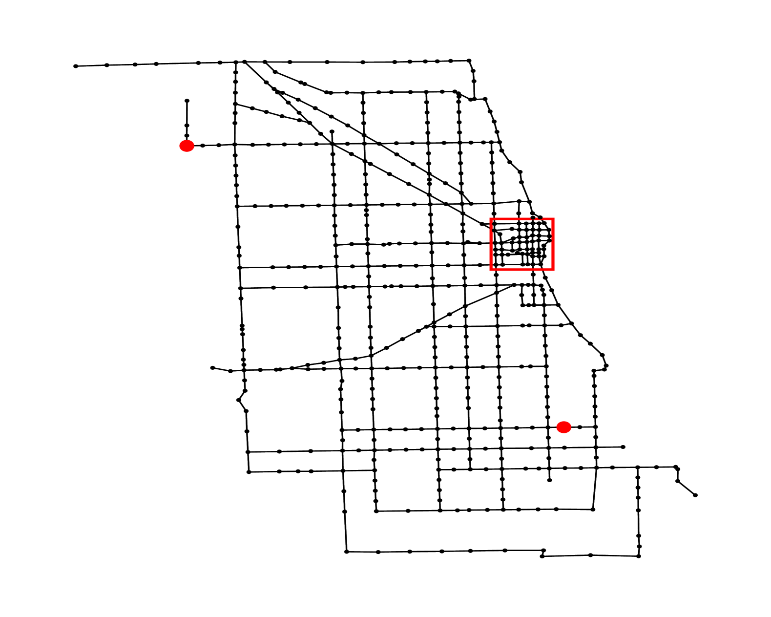
(a) Graph of a real road network in Chicago. The extracted city center scenario is marked by the red rectangle.

(b) Extracted graph of the city center of Chicago.

Figure 3. Used graphs for the experiments. The start and end point of the shortest path are marked in red.

Recall that the used framework aims at finding solutions for a new instance, while both optimizing the problem specific objective function as well as improving the explainability of the found solution. The explainability is based on the most similar instances from $S^{\leq}_{\epsilon}$. In other words, we seek a solution that aligns most closely with the solutions of the $k$ most similar instances while also remaining close to optimality. We set $k=5$ for the remainder of the section.

The role of features is crucial in determining the most similar instances. In [2], the distance metric is defined using all given input features, which in the presented experiments for the shortest path problem were edge weights of the graph. In the following experiments we show that it is beneficial to first select the most relevant features, before applying the framework.

To perform feature selection, we first require a comprehensive list of candidate features. For this purpose, we primarily utilized specific features that we call grid features. To this end, the graph was divided into a grid of rows and columns as shown in Figure 4. For each resulting cell, the weights of all edges whose midpoints fall within the cell were summed up. This ensures that every edge contributes to exactly one feature, providing a simple yet effective way to represent the graph’s structure.

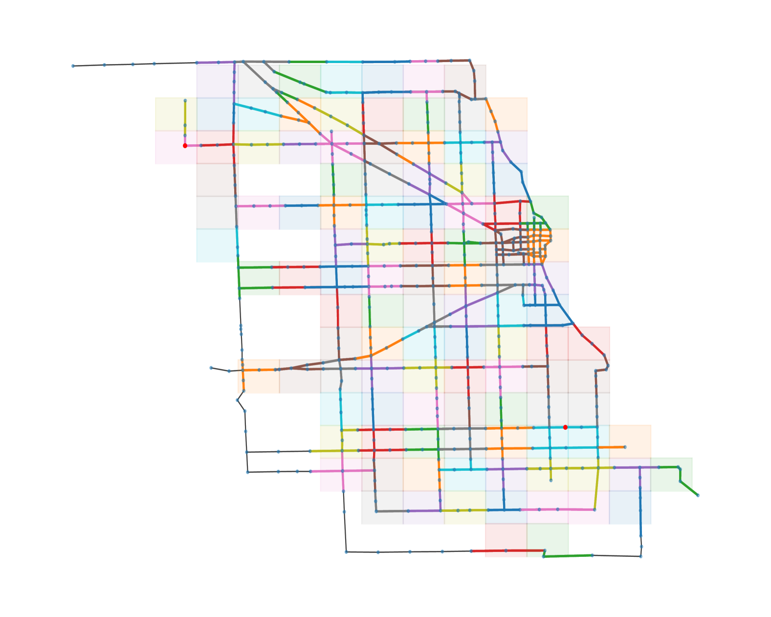
(a) Visualization of 110 grid features on the Chicago graph.

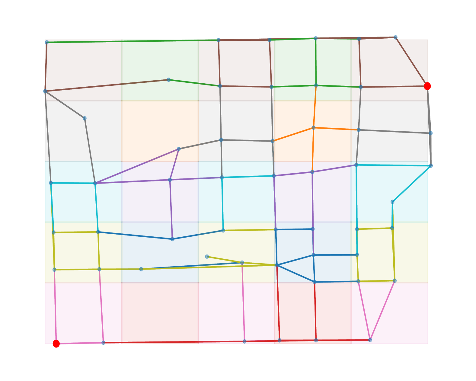
(b) Visualization of 20 grid features on the city center graph. Each edge is colored according to the grid cell that contains its midpoint.

Figure 4. Used grid features.

The grid dimensions were chosen individually for each scenario and experiment and will be further explained there. While finer grids provide more detailed features, they may diminish the explainability effect by fragmenting the representation. For our experiments this grid-based approach is sufficient. Additionally, unless otherwise specified, the individual edges were also included as potential features.

These feature values were stored in an instance feature vector. Additionally, a solution feature vector was created, represented as a binary vector. Each entry in this vector corresponds to an edge, taking the value 1 if the edge is part of the optimal solution for the graph and 0 otherwise. These vectors were then used in various feature selection approaches, ultimately yielding a list of $L$ selected features.

Since our primary focus is on the explainability effect, we do not consider the entire Pareto front in this evaluation but instead restrict our analysis to the optimization problem (WS-Exp) with $\alpha=0$. This parameter choice puts particular emphasis on distance features and is thus the most suitable choice to evaluate the methods presented here. Consequently, we focus on a solution that aligns most closely with the most similar instances in $S^{\leq}_{\epsilon}$ and then compute its relative length compared to the optimal path for that instance to assess the costs of explainability.

We retain the setting where all edges are selected as features as a benchmark in all plots. For the evaluation of the feature selection approaches, the only difference is the determination of $S^{\leq}_{\epsilon}$ where the feature functions $\phi_{\mathcal{I}}$ now only consider the features that were selected in the feature selection process.

In all plots, the $x$-axis represents the feature cardinality $L$ and the $y$-axis represents the relative length of the most explainable path. The red line represents results obtained by the original approach that uses all given weights as features. As an additional benchmark, we randomly selected $L$ features $100$ times for each instance set, and evaluated and averaged them as described above.

8.2. Computational Experiments

All computations were performed on a high-performance cluster using a Python implementation. The experiments were executed on a machine equipped with two Intel Xeon Gold 6326 (“Ice Lake”) processors, each featuring 2 $\times$ 16 cores clocked at 2.9 GHz. For solving the MIP models, we employed Gurobi 12.0.0.

Even for small problem sizes, it quickly became apparent that the FSP-EO (4) could not be solved to global optimality within reasonable time. To obtain results nonetheless, we reduced the problem size to $N=10$ instances of the city center graph per set, using only $2\times 3$ grid features. In this simplified setup, the FSP-EO can be solved optimally. Interestingly, in this setting, even the simplest case of the $K$-opt heuristic, the $K$-opt heuristic from Section 6 with a choice of $K=1$, consistently finds solutions that coincide with the optimal FSP-EO results. However, this observation is likely due to the simplicity of the scenario and does not necessarily generalize to more complex instances.

Since all $N$ instances in a set must be compared pairwise, the FSP-EO involves $2N^{2}$ big-M constraints. Although this complexity is substantial, the chosen number of instances allows for exact optimization. Nevertheless, the underlying problem remains NP-hard, so scalability quickly becomes a limiting factor.

When increasing the number of instances per set to $N=20$, the FSP-EO frequently exhibited a gap of 80–90% after one hour of computation. For smaller problem sizes, this is likely due to slow improvements in the dual bound, whereas for larger instances, the 1-opt heuristic consistently outperforms the best FSP-EO solutions obtained within the time limit. This indicates that the FSP-EO remains far from optimality in these cases. Similar challenges arise for the pessimistic FSP-EO (7) and the affine variant (9), both of which struggle to produce feasible solutions or exhibit prohibitively large optimality gaps. While we have not yet explored heuristic alternatives for the affine variant, the pessimistic FSP-EO can leverage the same 1-opt heuristic (with only a small change how to decide if two instances have equal distance) as its optimistic counterpart. Given these computational challenges, we focus our analysis on the heuristic approach, which provides reliable results within reasonable runtime.

In the first full-scale experiment, we again used the smaller city center graph but increased the number of instances per set to $N=200$. The feature list, from which $L$ features were to be selected, included $4\times 5$ grid features and additional edge features, resulting in a total of 121 candidate features. We chose the $4\times 5$ grid to strike a balance between meaningful feature representation and good explainability for the end user.

In Figure 5, we observe that even with this relatively small number of features, our approach of first selecting relevant features, often performs better than the original approach where costs of every single edge were used as features to find similar instances. Our approach not only produces better solutions but also enhances explainability, as the end-user compares only carefully selected features rather than all individual edge costs. The random feature selection as other benchmark to beat leads to the worst explainability values. A small number of meticulously selected features outperforms the full edge features benchmark.

Interestingly, the selected features frequently included a balanced mix of individual edges and grid features. This suggests that a well-designed combination of both feature types could provide the best explainability. While the grid features were initially placed at equidistant intervals, a more detailed analysis of the city’s structure could further refine their selection, potentially enhancing interpretability.

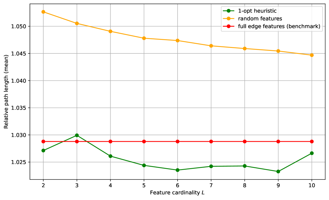
Figure 5. In the plot we see the relative length of the most explainable path as a function of the feature cardinality $L$. We have done a feature selection process on 10 sets out of $N=200$ instances of the city center graph. The feature list contained 20 grid features as well as all the edges.

To demonstrate this, we conducted the next experiment using the full Chicago graph. This time, the graph was divided into a $15\times 15$ grid, considering only the resulting grid features and excluding any edge features. Since many of these grid cells fall outside the graph, the feature candidate list consisted of 110 grid features. This grid size was chosen to achieve a similar number of features as in the city center graph experiment, ensuring comparability between the two setups.

In Figure 6, we observe that with these features, our approach currently cannot outperform the approach of using all costs as features. We still get close to the performance of the full edge features benchmark, but in this case we only have to look at the traffic volume of some regions instead of every single edge. This offers significantly higher explainability for the end user. Specifically, we can now provide insights such as, Focus on these regions of the city to compare traffic with other scenarios and identify optimal paths, rather than analyzing every single edge individually.

Figure 6. In the plot we see the relative length of the most explainable path as a function of the feature cardinality $L$. We have done a feature selection process on 10 sets out of $N=200$ instances of the complete Chicago graph. The feature list contained 110 grid features.

In the final experiment, we shift both the start and end points of the shortest path to the lower part of the graph. As a result, most edges in the upper region are never used for path selection, and their traffic load is likely uncorrelated with this section of the network (see Figure 7).

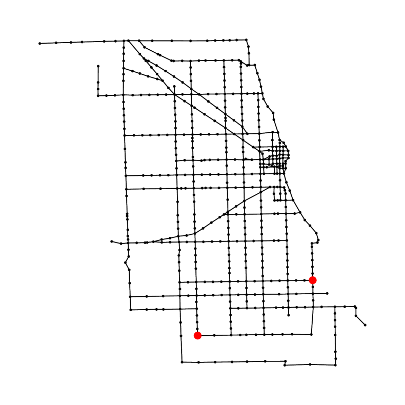
Figure 7. For this experiment, we again used the Chicago instance, but this time, the shortest path is determined between the two red dots in the lower half. As a result, the traffic in most of the network has little to no impact on the pathfinding process.

We use the same feature set as in the previous experiment, relying exclusively on grid features. However, in this setting, the feature selection approach outperforms the full edge features benchmark (see Figure 8). This is because it focuses only on features representing traffic in the relevant lower part of the graph, whereas the benchmark still evaluates the overall traffic distribution across the entire network.

This highlights the importance of feature selection in ensuring meaningful comparisons. Without it, irrelevant parts of the network—such as unused edges in this case—can distort the similarity assessment. By selecting only the most relevant features, we improve the explainability of the results and ensure that comparisons focus on the truly influential aspects of the network, leading to more reliable conclusions.

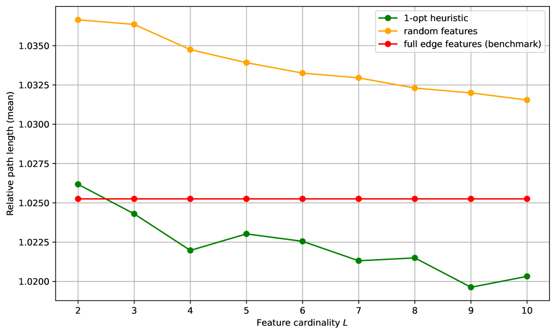
Figure 8. In the plot, we see the relative length of the most explainable path as a function of the feature cardinality $L$. This experiment considers only the shortest paths in the lower part of the graph, where many edges have little to no influence on the pathfinding process.

9. Conclusions and Outlook

Explainability of solutions is of key importance when applying optimization methods in practice. The best solution will, in the end, remain worthless if it is not accepted by practitioners. This paper picks up a recently introduced, data-driven concept of explainability in optimization and asks the question how to define features that are used to describe instances. We would like to pick a set of features that is not too large, so that they remain easily understandable. Furthermore, we should design them in a way that they are effective in the explanation process; in our context, this means that instance features are chosen so that similar instances lead to similar solutions.

To break ties between instances that have the same distance, we introduced an optimistic and pessimistic problem variant. We showed that both are NP-hard to solve, and introduced a mixed-integer programming formulation for each. Due to the problem hardness, we proposed a local search heuristic that iteratively exchanges features to improve the solution quality. A possible extension of this concept is to use affine combinations of features, which enables us to weight the importance of features against each other, and even put negative weight on them. While this approach makes the proposed framework more flexible, it also comes at the cost of a more involved mixed-integer programming formulation.

In extensive computational experiments using real-world shortest path data, we compared our feature selection approach with randomly chosen features and with an approach that measures differences on each edge of the graph as benchmarks. Our results show that by using far fewer features than the latter approach, we can obtain a comparable performance in our setting. Even more, if not all data in the instance is relevant, using all edges can even be misleading, and our approach outperforms the benchmark while using fewer features.

Several avenues for further research emerge. This paper only considered the side of instance features, which means that similar considerations for solution features remain open. Furthermore, we assume that a set of feature candidates is given, of which we select a small subset. In a further step, we may consider how to find such a set, i.e., generalize from feature selection problems towards feature generation problems, both for solution and for instance features. Finally, the proposed framework of explainability is a first step in this direction, but we believe that many alternative definitions of explainability are conceivable and should be studied in the future.

References

- AAV [19] Sina Aghaei, Mohammad Javad Azizi, and Phebe Vayanos. Learning optimal and fair decision trees for non-discriminative decision-making. Proceedings of the AAAI Conference on Artificial Intelligence, 33(01):1418–1426, Jul. 2019.
- AGH+ [24] Kevin-Martin Aigner, Marc Goerigk, Michael Hartisch, Frauke Liers, and Arthur Miehlich. A framework for data-driven explainability in mathematical optimization. Proceedings of the AAAI Conference on Artificial Intelligence, 38(19):20912–20920, Mar. 2024.
- BD [19] Peter Bugata and Peter Drotár. Weighted nearest neighbors feature selection. Knowledge-Based Systems, 163:749–761, 2019.
- BMS [98] Paul S Bradley, Olvi L Mangasarian, and W Nick Street. Feature selection via mathematical programming. INFORMS Journal on Computing, 10(2):209–217, 1998.
- CBC+ [25] GianCarlo A. P. I. Catalano, Alexander E. I. Brownlee, David Cairns, John A. W. McCall, Martin Fyvie, and Russell Ainslie. Explaining a staff rostering problem using partial solutions. In Max Bramer and Frederic Stahl, editors, Artificial Intelligence XLI, pages 179–193, Cham, 2025. Springer Nature Switzerland.
- CDG [19] André Chassein, Trivikram Dokka, and Marc Goerigk. Algorithms and uncertainty sets for data-driven robust shortest path problems. European Journal of Operational Research, 274(2):671–686, 2019.
- CGMS [24] Salvatore Corrente, Salvatore Greco, Benedetto Matarazzo, and Roman Slowiński. Explainable interactive evolutionary multiobjective optimization. Omega, 122:102925, 2024.
- ČLL [21] Kristijonas Čyras, Myles Lee, and Dimitrios Letsios. Schedule explainer: An argumentation-supported tool for interactive explanations in makespan scheduling. In International Workshop on Explainable, Transparent Autonomous Agents and Multi-Agent Systems, pages 243–259. Springer, 2021.
- ČLMT [19] Kristijonas Čyras, Dimitrios Letsios, Ruth Misener, and Francesca Toni. Argumentation for explainable scheduling. Proceedings of the AAAI Conference on Artificial Intelligence, 33(01):2752–2759, Jul. 2019.
- CMP [19] Anna Collins, Daniele Magazzeni, and Simon Parsons. Towards an argumentation-based approach to explainable planning. In ICAPS 2019 Workshop XAIP Program Chairs, 2019.
- CRAM [24] Emilio Carrizosa, Jasone Ramírez-Ayerbe, and Dolores Romero Morales. Mathematical optimization modelling for group counterfactual explanations. European Journal of Operational Research, 319(2):399–412, 2024.
- DA [22] Pradip Dhal and Chandrashekhar Azad. A comprehensive survey on feature selection in the various fields of machine learning. Applied Intelligence, 52(4):4543–4581, 2022.
- DBCDC+ [23] Koen W De Bock, Kristof Coussement, Arno De Caigny, Roman Slowiński, Bart Baesens, Robert N Boute, Tsan-Ming Choi, Dursun Delen, Mathias Kraus, Stefan Lessmann, et al. Explainable AI for operational research: A defining framework, methods, applications, and a research agenda. European Journal of Operational Research, 2023.
- DCD [24] Koen W. De Bock, Kristof Coussement, and Arno De Caigny. Explainable analytics for operational research. European Journal of Operational Research, 317(2):243–248, 2024.
- EK [21] Martin Erwig and Prashant Kumar. Explainable dynamic programming. Journal of Functional Programming, 31:e10, 2021.
- Fei [95] Uriel Feige. A threshold of for approximating set cover. Journal of the ACM, 45:634–652, 1995.
- FMC+ [23] Martin Fyvie, John AW McCall, Lee A Christie, Alexandru-Ciprian Zăvoianu, Alexander EI Brownlee, and Russell Ainslie. Explaining a staff rostering problem by mining trajectory variance structures. In International Conference on Innovative Techniques and Applications of Artificial Intelligence, pages 275–290. Springer, 2023.
- FPV [23] Alexandre Forel, Axel Parmentier, and Thibaut Vidal. Explainable data-driven optimization: From context to decision and back again. In International Conference on Machine Learning, pages 10170–10187. PMLR, 2023.
- GH [23] Marc Goerigk and Michael Hartisch. A framework for inherently interpretable optimization models. European Journal of Operational Research, 310(3):1312–1324, 2023.
- GHMS [24] Marc Goerigk, Michael Hartisch, Sebastian Merten, and Kartikey Sharma. Feature-based interpretable surrogates for optimization. arXiv preprint arXiv:2409.01869, 2024.
- JMB [20] Dominik Janzing, Lenon Minorics, and Patrick Blöbaum. Feature relevance quantification in explainable AI: A causal problem. In International Conference on artificial intelligence and statistics, pages 2907–2916. PMLR, 2020.
- JOZ [24] Erik Johannesson, James A Ohlson, and Sophia Weihuan Zhai. The explanatory power of explanatory variables. Review of Accounting Studies, 29:3053–3083, 2024.
- KBdH [24] Jannis Kurtz, Ş İlker Birbil, and Dick den Hertog. Counterfactual explanations for linear optimization. arXiv preprint arXiv:2405.15431, 2024.
- LBMR [24] Teddy Lazebnik, Svetlana Bunimovich-Mendrazitsky, and Avi Rosenfeld. An algorithm to optimize explainability using feature ensembles. Applied Intelligence, 54(2):2248–2260, 2024.
- LCW+ [17] Jundong Li, Kewei Cheng, Suhang Wang, Fred Morstatter, Robert P Trevino, Jiliang Tang, and Huan Liu. Feature selection: A data perspective. ACM computing surveys (CSUR), 50(6):1–45, 2017.
- LMMRC [19] Martine Labbé, Luisa I. Martínez-Merino, and Antonio M. Rodríguez-Chía. Mixed integer linear programming for feature selection in support vector machine. Discrete Applied Mathematics, 261:276–304, 2019. GO X Meeting, Rigi Kaltbad (CH), July 10–14, 2016.
- MALM [22] Giovanni Misitano, Bekir Afsar, Giomara Lárraga, and Kaisa Miettinen. Towards explainable interactive multiobjective optimization: R-ximo. Autonomous Agents and Multi-Agent Systems, 36(2):43, 2022.
- Nd [10] Minh Hoai Nguyen and Fernando de la Torre. Optimal feature selection for support vector machines. Pattern Recognition, 43(3):584–591, 2010.
- NGGDdC [25] Manuel Navarro-García, Vanesa Guerrero, María Durban, and Arturo del Cerro. Feature and functional form selection in additive models via mixed-integer optimization. Computers & Operations Research, 176:106945, 2025.
- ODV [20] Nir Oren, Kees van Deemter, and Wamberto W Vasconcelos. Argument-based plan explanation. In Knowledge Engineering Tools and Techniques for AI Planning, pages 173–188. Springer, 2020.
- RGG [19] Miao Rong, Dunwei Gong, and Xiaozhi Gao. Feature selection and its use in big data: challenges, methods, and trends. IEEE Access, 7:19709–19725, 2019.
- Rud [19] Cynthia Rudin. Stop explaining black box machine learning models for high stakes decisions and use interpretable models instead. Nature Machine Intelligence, 1(5):206–215, 2019.
- SMSV [24] Breno Serrano, Stefan Minner, Maximilian Schiffer, and Thibaut Vidal. Bilevel optimization for feature selection in the data-driven newsvendor problem. European Journal of Operational Research, 315(2):703–714, 2024.
- SSG [18] Roykrong Sukkerd, Reid Simmons, and David Garlan. Toward explainable multi-objective probabilistic planning. In 2018 IEEE/ACM 4th International Workshop on Software Engineering for Smart Cyber-Physical Systems (SEsCPS), pages 19–25. IEEE, 2018.
- TBBN [22] Kevin Tierney, Kaja Balzereit, Andreas Bunte, and Oliver Niehörster. Explaining solutions to multi-stage stochastic optimization problems to decision makers. In 2022 IEEE 27th International Conference on Emerging Technologies and Factory Automation (ETFA), pages 1–4. IEEE, 2022.
- WBC [21] Aidan Wallace, Alexander EI Brownlee, and David Cairns. Towards explaining metaheuristic solution quality by data mining surrogate fitness models for importance of variables. In Artificial Intelligence XXXVIII: 41st SGAI International Conference on Artificial Intelligence, AI 2021, Cambridge, UK, December 14–16, 2021, Proceedings 41, pages 58–72. Springer, 2021.
- YKK [24] William B Yates, Edward C Keedwell, and Ahmed Kheiri. Explainable optimisation through online and offline hyper-heuristics. ACM Transactions on Evolutionary Learning, 2024.
- ZTK [23] Shudian Zhao, Calvin Tsay, and Jan Kronqvist. Model-based feature selection for neural networks: A mixed-integer programming approach. In International Conference on Learning and Intelligent Optimization, pages 223–238. Springer, 2023.
- ZvZCH [22] Jan Zacharias, Moritz von Zahn, Johannes Chen, and Oliver Hinz. Designing a feature selection method based on explainable artificial intelligence. Electronic Markets, 32(4):2159–2184, 2022.