Abstract

In this work, we investigate the discovery reach of a new physics model, the Inert Doublet Model, at an $e^{+}e^{-}$ machine with centre-of-mass energies $\sqrt{s}$ of 240 and 365 GeV. Within this model, four additional scalar bosons ($H,\,A,\,H^{+}$ and $H^{-}$) are predicted. Due to an additional symmetry, the lightest new scalar, here chosen to be $H$, is stable and provides an adequate dark matter candidate. The search for pair production of the new scalars is investigated in final states with two electrons or two muons, in the context of the future circular collider proposal, FCC-ee. Building on previous studies in the context of the CLIC proposal, this analysis extends the search to detector-level objects, using a parametric neural network to enhance the signal contributions over the Standard Model backgrounds, and sets limits in the $M_{A}-M_{H}$ vs $M_{H}$ plane. With a total integrated luminosity of 10.8 (2.7)  ab^-1 for $\sqrt{s}=$240 (365) GeV, almost the entire phase-space available in the $M_{A}-M_{H}$ vs $M_{H}$ plane is expected to be excluded at 95% CL, reaching up to $M_{H}$$=110\,(165)$ GeV. The discovery reach is also explored, reaching $M_{H}$$=108\,(157)\,\text{G\text{eV}}$ for $M_{A}-M_{H}$$=15$ GeV  at $\sqrt{s}=$240 (365) GeV.

RBI-ThPhys-2025-08, CERN-TH-2025-069

[beforeskip=.2cm]sectionsection

1 Introduction

Despite the numerous cosmological observations pointing towards the existence of dark matter (DM) [1], the specific nature of DM is still an ever elusive mystery. This lack of understanding is further compounded by the fact that the abundance of DM is predicted to significantly outweigh that of normal matter. Assuming DM can interact directly with normal matter, it should be possible to detect it here on Earth. This can happen in a number of ways: DM passing through our solar system could directly interact with particles, imparting energy that can be detected in direct detection experiments; DM particles could modify Standard Model (SM) interactions and be detected indirectly through precision measurements; or, DM can be produced at a collider, leading for example to a missing energy signature. More details can be found in Ref. [1].

We consider the case in which DM particles are weakly interacting massive particles. A particle of this nature, however, is not contained in the SM, and as such alternatives theories — or extensions to the SM — are required to include this. In the context of extensions to the SM such as two-Higgs-doublet models, it is possible, via the addition of an exact $\mathbb{Z}_{2}$ symmetry, to make the lightest scalar boson from the additional doublet stable, and hence a suitable DM candidate. The study presented here considers a search for one such theory: the Inert Doublet Model (IDM) [2, 3, 4, 5, 6].

Although many phenomenological studies exist, dedicated studies of the IDM have not yet been performed by the experimental collaborations. Existing analyses are generally not sensitive to a large part of the parameter space due to too high requirements on the missing transverse energy, and their recast leads to very loose constraints (see e.g. discussion in [7]). In this paper, we present a search for the pair production of the extra scalars in $e^{+}e^{-}$ collisions at centre-of-mass energies ($\sqrt{s}$) of 240 and 365 GeV  in the context of the future circular collider of CERN, FCC-ee [8, 9, 10], using a final state with a pair of same-flavour leptons (electrons or muons).

This paper is organised as follows: the theoretical model is introduced in section 2. The signal and background Monte Carlo samples are detailed in section 3, with the object definitions given in section 4. Preselection and selection criteria that enhance the signal contribution and reject background processes are defined in section 5, and a multivariate analysis to further discriminate between signal and backgrounds is introduced in section 6. Finally, the results are given in section 7 and a conclusion in section 8.

2 The Inert Doublet Model

The Inert Doublet Model (IDM) is a two-Higgs-doublet model with an additional, unbroken $\mathbb{Z}_{2}$ symmetry. This model contains two scalar fields denoted $\phi_{D}$ and $\phi_{S}$, with the following transformation properties:

$$\mathbb{Z}_{2}:\quad\phi_{D}\longrightarrow-\phi_{D},\quad\quad\phi_{S}\longrightarrow\phi_{S},\quad\quad SM\longrightarrow SM.$$ (1)

With these field of the IDM, the most general, renormalisable scalar potential can be constructed:

$$\begin{split}V=-\frac{1}{2}[m^{2}_{11}(\phi_{S}^{\dagger}\phi_{S})+m^{2}_{22}(\phi_{D}^{\dagger}\phi_{D})]+\frac{\lambda_{1}}{2}(\phi_{S}^{\dagger}\phi_{S})^{2}+\frac{\lambda_{2}}{2}(\phi_{D}^{\dagger}\phi_{D})^{2}\\ \quad+\lambda_{3}(\phi_{S}^{\dagger}\phi_{S})(\phi_{D}^{\dagger}\phi_{D})+\lambda_{4}(\phi_{S}^{\dagger}\phi_{D})(\phi_{D}^{\dagger}\phi_{S})+\frac{\lambda_{5}}{2}[(\phi_{S}^{\dagger}\phi_{D})^{2}+(\phi_{D}^{\dagger}\phi_{S})^{2}].\end{split}$$ (2)

Due to the additional symmetry, electroweak symmetry breaking proceeds as in the SM. After symmetry breaking, the model contains in total seven free parameters. A suitable choice for these is e.g.

$$v,\,M_{h},\,M_{H},\,M_{A},\,M_{H^{\pm}},\,\lambda_{2},\,\lambda_{345}\,\equiv\,\lambda_{3}+\lambda_{4}+\lambda_{5},$$

where $v$ and $M_{h}$ are the vacuum expectation value (vev) and mass stemming from the SM-like doublet and are fixed through experimental measurements to $v\,\sim\,246\,\text{G\text{eV}}$ and $M_{h}\,\sim\,125\,\text{G\text{eV}}$, respectively. $H,\,A,$ and $H^{\pm}$ denote the novel so-called dark scalars, and $\lambda_{i}$ are couplings in the potential with $\lambda_{345}\equiv\lambda_{3}+\lambda_{4}+\lambda_{5}$. Here, $\lambda_{2}$ is the coupling constant for the quartic vertex between four IDM particles, and $\lambda_{345}$ is the coupling constant for the vertex between IDM particles and the SM Higgs boson. The couplings between the new scalars and the SM gauge bosons are determined solely by quantities from the SM electroweak sector. It should be noted that the scalars from the two doublets do not mix due to the $\mathbb{Z}_{2}$ symmetry, therefore there are no additional mixing parameters.

The $\mathbb{Z}_{2}$ symmetry leads to multiple interesting phenomenological features. First, the symmetry forbids any direct coupling between the IDM particles and the SM fermion fields, and as such the IDM particles only couple directly to bosons. Second, the symmetry requires that all terms in the Lagrangian involving IDM fields have an even number of IDM fields (2 or 4). As the second doublet does not acquire a vacuum expectation value, the symmetry remains exact and IDM particles are always produced in pairs. Finally, it also causes the lightest of the IDM particles to be stable and therefore a suitable DM candidate. In principle, any of the additional scalars can serve as a DM candidate. We here chose $H$, which automatically implies a mass hierarchy $M_{A}$,$M_{H^{\pm}}$$>$$M_{H}$.

Given that the IDM particles do not couple to the SM fermions, a typical signature at a collider is that of SM electroweak gauge boson plus missing energy, where the latter stems from the DM candidates. In addition, the model can also render monojet and monophoton signatures [12, 13] as well as processes containing the invisible decay of the 125 GeV SM-like scalar. This analysis focusses on the same-flavour dilepton (electrons or muons) plus missing energy final state, with example production mechanisms shown in figure 1.

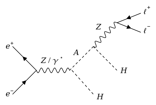
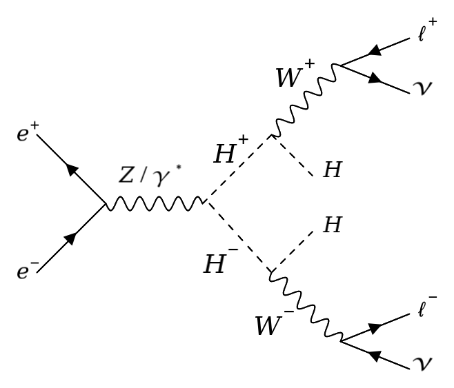
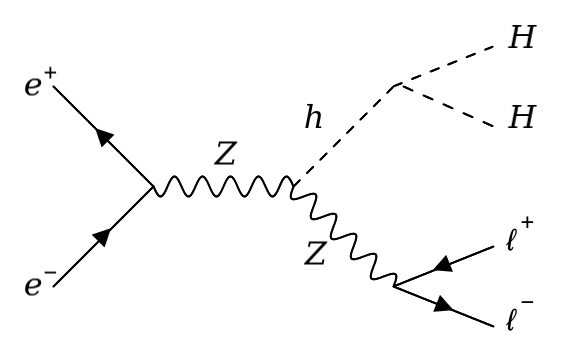
Figure 1: Leading-order Feynman diagrams of: (left) $HH\ell^{+}\ell^{-}$ production, (middle) $HH\ell^{+}\ell^{-}\nu\bar{\nu}$ production, and (right) $\mathup{{{Z}}}h\rightarrow HH\ell^{+}\ell^{-}$ production, with $\ell=e,\mu,\tau$.

The IDM is subject to a large number of theoretical and experimental constraints. In this work, we follow the scan presented in Ref. [14], with more recent updates presented in Refs [15, 16, 7, 11, 17]. In particular, we include constraints on the potential stemming from vacuum stability, perturbativity and perturbative unitarity, as well as electroweak precision observables (EWPO), evaluated through the publicly available tool 2HDMC [18, 19]. Results for the electroweak precision constraints are tested using the oblique parameters $S,\,T,\,U$ [20, 21, 22, 23] and comparing to the latest PDG values [1]. We also require that the parameter point resides in the inert vacuum [24]. We furthermore test for the most recent bound on SM Higgs boson decays to invisible particles in cases where this decay is allowed onshell, $\text{BR}\left(h\,\rightarrow\,\text{inv}\right)\,\leq\,0.11$ [25]. Regarding dark matter constraints, we calculate the predictions using Micromegas [26] and require agreement with the upper bound for relic density as measured by the Planck experiment [27]. Direct detection constraints are taken from the LuxZeplin collaboration [28]. Finally, we also make sure the mass hierarchy obeys the constraints from a recast of searches for supersymmetric neutralinos at LEP reinterpreted within the IDM [29] (referred to as LEP SUSY recast in the following), and that the particles would not contribute to the decay widths of the electroweak gauge bosons at leading order. In the remainder of this document, we will label points as allowed that fulfill all above constraints, if not mentioned otherwise. More details on the scan setup and the applied constraints can be found in the references above.

A set of benchmark points (BPs) were evaluated in Ref. [16] to identify representative regions of the phase space where the production is still allowed by existing constraints. For the analysis targeting only the same-flavour dilepton final state, the signal cross section is usually dominated by the $AH$ production, and the sensitivity will depend mostly on $M_{H}$ and $M_{A}-M_{H}$. Instead of just estimating the sensitivity on the benchmark points, we adopt a strategy to scan the parameter space in $M_{H}$ and $M_{A}-M_{H}$, with several scenarios described below to study the dependency on the other parameters: $M_{H^{\pm}}$, $\lambda_{2}$ and $\lambda_{345}$.

Diagrams involving quartic couplings between IDM scalar bosons do not participate to the production of the final state under study. Hence, there is no sensitivity to the $\lambda_{2}$ coupling, which is set to 0.1 everywhere. Concerning diagrams involving the coupling $\lambda_{345}$ of the new scalars with the SM $h$ (see Fig. 1 right) two scenarios are considered: one where $\lambda_{345}=0$ and one where $\lambda_{345}$ is set to a relatively large value estimated using a linear parametrisation in $M_{H}$, $\lambda_{345}=0.0018\,\times\,\left(M_{H}-72\,\text{G\text{eV}}\right)$. This parametrisation is chosen to approach the maximal value allowed given recent results on direct detection searches for dark matter. As DM bounds in addition depend on the mass of the unstable neutral scalar, $M_{A}$, the actual maximal value might be lower than the one given by this parametrisation.

Similarly, we investigate two scenarios that differ in the choice of $M_{H^{\pm}}$: one with $M_{H^{\pm}}$$=$$M_{A}$, and one with $M_{H^{\pm}}$$-$$M_{A}$set to be within the maximum value allowed. Maximal mass splittings are in general mainly constrained from requiring perturbative unitarity as well as electroweak precision data. Note, however, that the latter also depends on the absolute mass scale. In order to estimate the maximally allowed mass differences, we first perform a random scan where we fix $\lambda_{2}$ but let all other parameters float. The resulting allowed parameter space is shown in figure 2. The points that have been simulated according to the fixed mass differences discussed above are displayed in green. As the absolute scale also plays a role in the determination of the oblique parameters, some points we chose, although overlaying with the allowed regions of a general scan, are forbidden by EWPO for specific choices of mass differences. These are displayed in red, but we chose to keep them for the final result for consistency reasons.

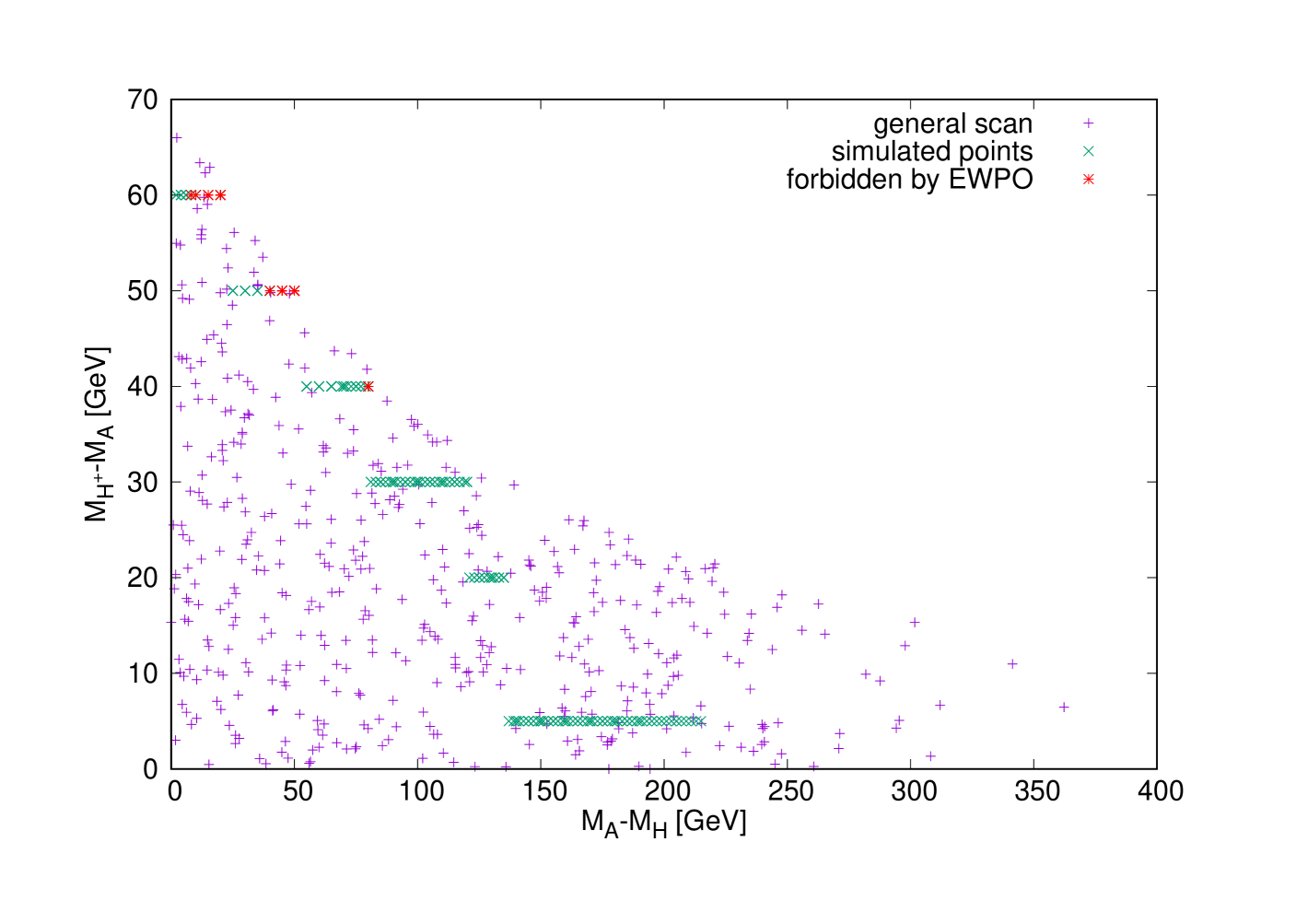
Figure 2: Allowed points in a general scan with $\lambda_{2}\,=\,0.1$ (purple, $+$), as well as points used in the simulation (green, x). Some of the latter are forbidden by electroweak precision observable constraints, which were implemented via the oblique parameters $S,\,T,\,U$ (red, $*$).

To summarise, three different scenarios are considered, where we vary $M_{H}$ and $M_{A}$, and set $\lambda_{345}$ and $M_{H^{\pm}}$to specific values:

• (S1) $M_{H^{\pm}}$$=$$M_{A}$ and $\lambda_{345}=0$;

• (S2) $M_{H^{\pm}}$$=$$M_{A}$ and $\lambda_{345}$ close to the maximum value allowed, referred to as $\lambda_{max}$; this scenario is meant to test the impact of production through the SM $h$ (see Fig. 1 right);

• (S3) within maximum $M_{H^{\pm}}$, referred to as $M_{H^{\pm}}^{max}$, and $\lambda_{max}$; this scenario is meant to test the contribution of the $H^{+}H^{-}$ production (see Fig. 1 middle).

3 Monte Carlo samples

The IDM signal samples are generated using MADGRAPH5_aMC@NLO v2.8.1 [30] interfaced with PYTHIA v8.2 [31], using $e^{+}e^{-}$ collisions at $\sqrt{s}=$240 and 365 GeV. The input UFO [32] model is taken from Ref. [33]. Instead of targeting individual pair production modes, two final states are generated directly, therefore taking into account all contributing diagrams and the proper interferences. The two final states we consider here are given by $HH\ell\ell$ and $HH\ell\ell\nu\nu$, with $\ell=e$, $\mu$ or $\tau$, and $H$ the stable dark scalar. The lepton charges are omitted in the notations. The $\tau$ leptons are decayed by PYTHIA. Typically, the former final state is obtained with a virtual or real $\mathup{{{Z}}}$ boson (Fig. 1 left), and the sensitivity will roughly depend on the mass difference between $H$ and $A$. The latter final state is mediated via a pair of $\mathup{{{W}}}$ bosons (Fig. 1 middle) and the sensitivity will instead depend on the difference in mass between $H$ and the charged scalars. The signal is generated fixing the coupling $\lambda_{2}$ to 0.1, $M_{H}$ between 70 and 115 (180) GeV in steps of 5 GeV for $\sqrt{s}$ =$240\,(365)\,\text{G\text{eV}}$, and $M_{A}-M_{H}$ between 2 GeV and the kinematic limit for on-shell production in steps of 2 to 5 GeV. Three scenarios are considered for setting $M_{H^{\pm}}$ and $\lambda_{345}$, as detailed in section 2, and 500,000 events are generated per point. The cross section values are shown in Figs. 3 and  4 in the simulated $M_{A}-M_{H}$ vs. $M_{H}$ grid plane for $\sqrt{s}=$240 and 365 GeV respectively, on the left for the $HH\ell\ell$ final state and on the right for the $HH\ell\ell\nu\nu$ final state, for the scenario S1. For the number of events generated, the Monte Carlo (MC) integration error for the cross sections is typically smaller than 0.1%. The minimum transverse momentum of the leptons, $p_{\mathrm{T}}^{\ell}$, is set at 0.5 GeV.

Figure 3: Cross section from the MG5_aMC@NLO simulation at $\sqrt{s}=$240 GeV, for the points simulated in the $M_{A}-M_{H}$ vs $M_{H}$ plane in scenario S1. All cross sections are in fb, computed for $p_{\mathrm{T}}^{\ell}>0.5$ GeV and with a numerical integration error smaller than 0.1%. Left: $HH\ell\ell$ final state, right: $HH\ell\ell\nu\nu$ final state. The dashed line shows the kinematic limit for on-shell production.

Figure 4: Cross section from the MG5_aMC@NLO simulation at $\sqrt{s}=$365 GeV, for the points simulated in the $M_{A}-M_{H}$ vs $M_{H}$ plane in scenario S1. All cross sections are in fb, computed for $p_{\mathrm{T}}^{\ell}>0.5$ GeV and with a numerical integration accuracy smaller than 0.1%. Left: $HH\ell\ell$ final state, right: $HH\ell\ell\nu\nu$ final state. The dashed line shows the kinematic limit for on-shell production.

Almost no difference is found between S2 and S1, which is expected from the range of $M_{H}$ values of interest here, $M_{H}$$>$$M_{h}$$/2$. The largest differences are for S3 in the $HH\ell\ell\nu\nu$ final state, for which $M_{H^{\pm}}$ drives the cross section. The cross section ratios between S3 and S2 are shown in Fig. 5 in the $M_{A}-M_{H}$ vs. $M_{H}$ plane for $\sqrt{s}=$240 GeV (left) and $\sqrt{s}=$365 GeV (right) for the $HH\ell\ell\nu\nu$ final state.

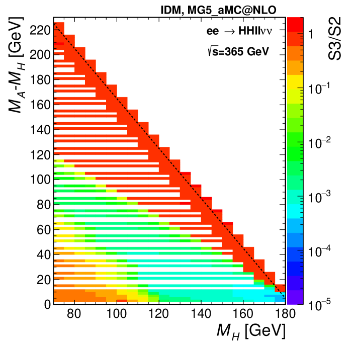
Figure 5: Cross section ratios S3/S2 in the $M_{A}-M_{H}$ vs $M_{H}$ plane, from the MG5_aMC@NLO simulation at $\sqrt{s}=$240 GeV (left) and $\sqrt{s}=$365 GeV (right), for the $HH\ell\ell\nu\nu$ final state. The dashed line shows the kinematic limit.

Background processes include diboson production ($\mathup{{{\mathup{{{W}}}}}^{\scriptstyle{+}}}\mathup{{{\mathup{{{W}}}}}^{\scriptstyle{-}}}$ and $\mathup{{{Z}}}\mathup{{{Z}}}$), inclusive $ee$, $\mu\mu$ and $\tau\tau$ production, SM Higgs boson production in association with a $\mathup{{{Z}}}$ boson, and $\mathup{{{t}}}\mathup{{\overline{{\mathup{{{t}}}}}}}$ production at $\sqrt{s}=$365 GeV. Samples were produced centrally with high statistics, within the so-called Winter2023 campaign [34], as given in Table 1 for $\sqrt{s}=$240 GeV and in Table 2 for $\sqrt{s}=$365 GeV, using PYTHIA v8.306 [35] for the diboson and $\mathup{{{t}}}\mathup{{\overline{{\mathup{{{t}}}}}}}$ samples, and WHIZARD v3.0.3 [36] interfaced with PYTHIA v6.4.28 [37] for the other processes. For the inclusive $ee$ production, a lower limit of 30 GeV is set on the invariant mass of the pair of electrons produced. The dielectron channel is hence included in the analysis only in the parameter space where the background is simulated, namely for $M_{A}-M_{H}$$>30$ GeV.

The current target values for the total integrated luminosities of the $\sqrt{s}=$240 and 365 GeV FCC-ee runs are 10.8 and 2.7  ab^-1, respectively [38].

Both signal and background samples are processed through DELPHES v3.5.1pre05 [39] with the IDEA [40] detector configuration as per the Winter2023 campaign. Events are produced using the KEY4HEP [41] framework and analysed using the FCCAnalyses package [42].

Process	N generated	cross section (pb)	Eq. $\mathcal{L}$ (ab-1)
$\mathup{{{Z}}}\mathup{{{Z}}}$	56162093	1.359	41
$\mathup{{{\mathup{{{W}}}}}^{\scriptstyle{+}}}\mathup{{{\mathup{{{W}}}}}^{\scriptstyle{-}}}$	373375386	16.4385	23
$\mathup{{{Z}}}$($ee$)$h$	1200000	0.00716	168
$\mathup{{{Z}}}$($\mu\mu$)$h$	1200000	0.00676	178
$\mathup{{{Z}}}$($\tau\tau$)$h$	1200000	0.00675	178
$\mathup{{{Z}}}$($\nu\nu$)$h$	3500000	0.0462	76
$\mathup{{{Z}}}$($\mathrm{q}\bar{\mathrm{q}}$)$h$	6700000	0.136	49
$ee$ $30<M_{ee}<150$ GeV	85400000	8.305	10
$\mu\mu$	53400000	5.288	10
$\tau\tau$	52400000	4.668	11

Table 1: Background processes generated in the Winter2023 campaign at $\sqrt{s}=$240 GeV. $\mathup{{{Z}}}\mathup{{{Z}}}$ and $\mathup{{{\mathup{{{W}}}}}^{\scriptstyle{+}}}\mathup{{{\mathup{{{W}}}}}^{\scriptstyle{-}}}$ are generated using Pythia8, whilst the others are generated with Whizard+Pythia6. The last column gives the total integrated luminosity simulated.

Process	N generated	cross section (pb)	Eq. $\mathcal{L}$ (ab-1)
$\mathup{{{Z}}}\mathup{{{Z}}}$	11470944	0.6428	18
$\mathup{{{\mathup{{{W}}}}}^{\scriptstyle{+}}}\mathup{{{\mathup{{{W}}}}}^{\scriptstyle{-}}}$	11754213	10.7165	1.1
$\mathup{{{Z}}}$($ee$)$h$	1000000	0.00739	135
$\mathup{{{Z}}}$($\mu\mu$)$h$	1200000	0.004185	287
$\mathup{{{Z}}}$($\tau\tau$)$h$	1100000	0.004172	264
$\mathup{{{Z}}}$($\nu\nu$)$h$	2200000	0.05394	41
$\mathup{{{Z}}}$($\mathrm{q}\bar{\mathrm{q}}$)$h$	2400000	0.032997	73
$ee$ $30<M_{ee}<150$ GeV	3000000	1.527	2.0
$\mu\mu$	6600000	2.2858	2.9
$\tau\tau$	12800000	2.01656	6.3
$\mathup{{{t}}}\mathup{{\overline{{\mathup{{{t}}}}}}}$	2700000	0.8	3.4

Table 2: Background processes generated in the Winter2023 campaign at $\sqrt{s}=$365 GeV. $\mathup{{{Z}}}\mathup{{{Z}}}$, $\mathup{{{\mathup{{{W}}}}}^{\scriptstyle{+}}}\mathup{{{\mathup{{{W}}}}}^{\scriptstyle{-}}}$ and $\mathup{{{t}}}\mathup{{\overline{{\mathup{{{t}}}}}}}$ are generated using Pythia8, whilst the others are generated with Whizard+Pythia6. The last column gives the total integrated luminosity simulated.

4 Definition of the objects in Delphes

The origin of the coordinate system adopted in this work is defined as having the origin centered at the nominal collision point inside the experiment. The y-axis points vertically upward, and the x-axis points radially inward toward the centre of the FCC. Thus, the z-axis points along the beam direction. The azimuthal angle $\phi$ is measured from the x-axis in the x-y plane. The polar angle $\theta$ is measured from the z-axis. Pseudorapidity is defined as $\eta=-\ln\left[\tan(\theta/2)\right]$. The momentum and energy are denoted by $p$ and $E$, respectively. Those transverse to the beam direction, denoted by $p_{\text{T}}$ and $E_{\text{T}}$, respectively, are computed from the x and y components. The imbalance of energy is denoted by $E^{miss}$, and that measured in the transverse plane by $E_{\text{T}}^{miss}$.

The parametrisation of the reconstructed objects in Delphes is summarised in Table 3. The resolution smearing for the calorimeters is defined as

$$\sigma_{E}=\sqrt{E^{2}\times c+E\times s+n}$$

with $c=0.005$ (0.01) the constant term, $s=0.03$ (0.3) GeV^1/2 the sampling term and $n=0.002$ (0.05) GeV the noise term for the electromagnetic (hadronic) parts.

Algorithm	Objects	Selection requirements	efficiency
Tracking	$e$, $\mu$, charged hadrons	$p_{\text{T}}$ $>0.1$ GeV, $|\eta|<2.56$	1
Identification	$\gamma$, $e$, $\mu$	$E>2$ GeV, $|\eta|<3$	0.99

Table 3: Efficiency and selection requirements implemented in the Delphes card for the IDEA detector configuration.

At preselection, a minimum momentum requirement of $p>5$ GeV is imposed on the Delphes reconstructed electrons, muons and photons. Events with exactly two such electrons or exactly two such muons are selected for analysis.

Jets are reclustered from Delphes reconstructed particles after removing the selected electron and muon candidates. The Durham algorithm is used, with exclusive clustering of two jets, and an energy-based scheme [43]. The missing energy is taken as given by Delphes, where the DM candidates count as invisible particles.

5 Background rejection

5.1 Selection

To remain fully sensitive to all signal points but significantly reduce the background contributions, the following preselection criteria are applied, which are inspired from previous studies performed at generator level with the CLIC setup [44, 45].

Only events with exactly two same-flavour leptons $\ell=e$ or $\mu$, $M_{\ell\ell}<120$ GeV, $|p_{z}(\ell\ell)|<70$ GeV are kept. For the $\sqrt{s}=$365 GeV setup, for several benchmark points the signal contribution has $M_{\ell\ell}$ values well above the Z invariant mass. In order to more efficiently reject the backgrounds, the selection is modified to $|p_{z}(\ell\ell)|<140$ GeV, and the selection in $M_{\ell\ell}$ is chosen to be dependent on $p_{z}(\ell\ell)$, with the formula: $M_{\ell\ell}<(-9.0/14.0\times|p_{z}(\ell\ell)|+200)$, with $M_{\ell\ell}$ and $p_{z}(\ell\ell)$ in GeV. As an example, the distribution of $M_{\mu\mu}$ as a function of $p_{z}(\mu\mu)$ is shown for the sum of the major backgrounds and a few signal representative benchmark points from Ref. [44] in Fig. 6, for $\sqrt{s}=$240 (365) GeV on the left (right). A good agreement is found with the results obtained using the CLIC setup.

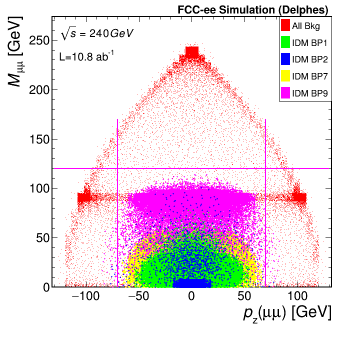
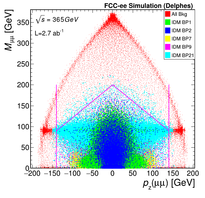
Figure 6: Dimuon mass $M_{\mu\mu}$ as a function of the dimuon $p_{z}(\mu\mu)$, for the selection of a muon pair with $e^{+}e^{-}$ collisions at $\sqrt{s}=$240 (365) GeV on the left (right). The sum of the background processes is shown in red. Several representative signal benchmark points are shown in green (BP1), blue (BP2), yellow (BP7) and pink (BP9). On the right, also BP21 is shown in cyan. The specification of the BPs can be found in Ref. [44]. The pink lines highlight the selection requirements.

With a negligible impact on the signal efficiency, the $ee\rightarrow\ell\ell,\,\tau\tau$ background is further reduced by 90% if requiring the transverse missing energy $E_{\text{T}}^{miss}$ $>5$ GeV. As no additional object is expected for signal events, a veto is applied on events with any additional electron or muon, any photon $E>5$ GeV or any jet. To further reject background, only events with the leading (subleading) lepton $p_{\text{T}}$ $<80$ (60) GeV are kept for $\sqrt{s}=$240 GeV, $p_{\text{T}}$ $<140$ (80) GeV for $\sqrt{s}=$365 GeV. Finally, events with $p_{\ell\ell}/E_{\ell\ell}>0.1$ are selected. All selection criteria are summarised in Table 4.

Step	Selection at $\sqrt{s}=$240 GeV	Selection at $\sqrt{s}=$365 GeV	target background
Preselection	$|p_{z}(\ell\ell)|<70$ GeV	$|p_{z}(\ell\ell)|<140$ GeV	$\mathup{{{Z}}}\mathup{{{Z}}}$, $ee\rightarrow\ell\ell$
	$M_{\ell\ell}<120$ GeV	$M_{\ell\ell}<(-9.0/14.0\times|p_{z}(\ell\ell)|+200)$	$\mathup{{{\mathup{{{W}}}}}^{\scriptstyle{+}}}\mathup{{{\mathup{{{W}}}}}^{\scriptstyle{-}}}$, $ee\rightarrow\ell\ell$
	$E_{\text{T}}^{miss}$ $>5$ GeV		$\mathup{{{Z}}}\mathup{{{Z}}}$, $ee\rightarrow\ell\ell$
Object veto	3rd lepton $E>5$ GeV, jet, photon $E>5$ GeV		$\mathup{{{\mathup{{{W}}}}}^{\scriptstyle{+}}}\mathup{{{\mathup{{{W}}}}}^{\scriptstyle{-}}}$, $\mathup{{{Z}}}\mathup{{{Z}}}$, $ee\rightarrow\ell\ell,\,\tau\tau$
Leptons $p_{\text{T}}$	$p_{\text{T}}$ $<80,60$ GeV	$p_{\text{T}}$ $<140,80$ GeV	$\mathup{{{\mathup{{{W}}}}}^{\scriptstyle{+}}}\mathup{{{\mathup{{{W}}}}}^{\scriptstyle{-}}}$, $\mathup{{{Z}}}\mathup{{{Z}}}$, $ee\rightarrow\tau\tau$
E/p	$p_{\ell\ell}/E_{\ell\ell}>0.1$		$ee\rightarrow\ell\ell,\,\tau\tau$

Table 4: Summary of the selection criteria and target backgrounds. Here $\ell$ is used for either electron or muon.

Just from requiring a pair of same-flavour leptons, 16% (4%) of $\mathup{{{Z}}}\mathup{{{Z}}}$ ($\mathup{{{\mathup{{{W}}}}}^{\scriptstyle{+}}}\mathup{{{\mathup{{{W}}}}}^{\scriptstyle{-}}}$) events are selected, further reduced to 5% (2%) after preselection, and 1.5% (1%) after the veto on other objects and final set of selection criteria. For the dilepton production, the preselection achieves 99% (94%) rejection of $ee$ events in the $ee$ channel for $\sqrt{s}=$240 (365) GeV, 99% for the $\mu\mu$ in $\mu\mu$ channels, and 97% for the $\tau\tau$ events in both channels. The object veto and other selection criteria reduce the $ee$, $\mu\mu$ and $\tau\tau$ backgrounds by another factor of about 40%, 70% and 35%, respectively. For the signal, after requiring a pair of same-flavour leptons with $p>5$ GeV  only 2% (0.1%) of events are selected at low mass splitting $M_{A}-M_{H}$, increasing to about 65% (6%) at higher mass splitting, for the production of $HH\ell\ell$ ($HH\ell\ell\nu\nu$) in the scenario S1.

The final number of events expected after selection are given in Table 5 with the MC statistical uncertainty, for the different background processes and several representative signal points from the scenario S1, normalised to the total integrated luminosity values of the FCC-ee runs at $\sqrt{s}=$240 and 365 GeV, namely 10.8 and 2.7  ab^-1.

Process	$ee$ $\sqrt{s}=$240 GeV	$\mu\mu$ $\sqrt{s}=$240 GeV	$ee$ $\sqrt{s}=$365 GeV	$\mu\mu$ $\sqrt{s}=$365 GeV
Background processes
$\mathup{{{Z}}}\mathup{{{Z}}}$	9.74e+04 $\pm$ 1.60e+02	1.09e+05 $\pm$ 1.69e+02	9.30e+03 $\pm$ 3.75e+01	1.05e+04 $\pm$ 3.98e+01
$\mathup{{{\mathup{{{W}}}}}^{\scriptstyle{+}}}\mathup{{{\mathup{{{W}}}}}^{\scriptstyle{-}}}$	8.02e+05 $\pm$ 6.18e+02	8.72e+05 $\pm$ 6.44e+02	8.75e+04 $\pm$ 4.64e+02	9.32e+04 $\pm$ 4.79e+02
$\mathup{{{t}}}\mathup{{\overline{{\mathup{{{t}}}}}}}$	-	-	0	0
$ee$	6.16e+05 $\pm$ 8.05e+02	0	1.34e+05 $\pm$ 4.30e+02	0
$\mu\mu$	0	9.80e+04 $\pm$ 3.24e+02	0	2.86e+04 $\pm$ 1.64e+02
$\tau\tau$	4.92e+05 $\pm$ 6.88e+02	4.80e+05 $\pm$ 6.80e+02	5.83e+04 $\pm$ 1.57e+02	5.65e+04 $\pm$ 1.55e+02
$\mathup{{{Z}}}$($ee$)$h$	1.11e+02 $\pm$ 2.68e+00	0	1.88e+01 $\pm$ 6.13e-01	9.98e-02 $\pm$ 4.46e-02
$\mathup{{{Z}}}$($\mu\mu$)$h$	6.09e-02 $\pm$ 6.09e-02	1.33e+02 $\pm$ 2.85e+00	9.42e-03 $\pm$ 9.42e-03	1.74e+01 $\pm$ 4.05e-01
$\mathup{{{Z}}}$($\nu\nu$)$h$	2.15e+03 $\pm$ 1.75e+01	2.25e+03 $\pm$ 1.79e+01	6.08e+02 $\pm$ 6.34e+00	6.72e+02 $\pm$ 6.67e+00
$\mathup{{{Z}}}$($\tau\tau$)$h$	1.62e+01 $\pm$ 9.93e-01	1.90e+01 $\pm$ 1.08e+00	2.41e+00 $\pm$ 1.57e-01	2.11e+00 $\pm$ 1.47e-01
$\mathup{{{Z}}}$($\mathup{{{q}}}\mathup{{\overline{{\mathup{{{q}}}}}}}$)$h$	0	0	0	0
Representative signal mass points
70-76 $HH\ell\ell$	6.31e+03 $\pm$ 4.16e+01	7.07e+03 $\pm$ 4.41e+01	-	-
70-76 $HH\ell\ell\nu\nu$	1.24e+03 $\pm$ 2.33e+01	1.45e+03 $\pm$ 2.53e+01	-	-
80-150 $HH\ell\ell$	1.67e+03 $\pm$ 4.55e+00	1.86e+03 $\pm$ 4.80e+00	-	-
80-150 $HH\ell\ell\nu\nu$	3.06e-05 $\pm$ 7.42e-06	3.96e-05 $\pm$ 8.44e-06	-	-
100-134 $HH\ell\ell$	8.18e+02 $\pm$ 2.25e+00	8.94e+02 $\pm$ 2.35e+00	-	-
100-134 $HH\ell\ell\nu\nu$	1.14e-06 $\pm$ 6.59e-07	3.81e-07 $\pm$ 3.81e-07	-	-
100-104 $HH\ell\ell$	-	-	1.09e+02 $\pm$ 1.59e+00	1.39e+02 $\pm$ 1.80e+00
100-104 $HH\ell\ell\nu\nu$	-	-	1.96e+01 $\pm$ 1.00e+00	1.96e+01 $\pm$ 1.00e+00
120-231 $HH\ell\ell$	-	-	1.25e+02 $\pm$ 3.47e-01	1.41e+02 $\pm$ 3.68e-01
120-231 $HH\ell\ell\nu\nu$	-	-	2.61e-04 $\pm$ 7.59e-06	2.07e-04 $\pm$ 6.77e-06
125-215 $HH\ell\ell$	-	-	3.14e+02 $\pm$ 8.65e-01	3.53e+02 $\pm$ 9.18e-01
125-215 $HH\ell\ell\nu\nu$	-	-	1.23e-02 $\pm$ 1.14e-04	9.92e-03 $\pm$ 1.03e-04
140-200 $HH\ell\ell$	-	-	3.42e+02 $\pm$ 9.29e-01	3.80e+02 $\pm$ 9.79e-01
140-200 $HH\ell\ell\nu\nu$	-	-	1.31e-02 $\pm$ 1.21e-04	1.06e-02 $\pm$ 1.09e-04
160-185 $HH\ell\ell$	-	-	2.19e+02 $\pm$ 6.29e-01	2.39e+02 $\pm$ 6.56e-01
160-185 $HH\ell\ell\nu\nu$	-	-	3.61e-03 $\pm$ 4.81e-05	2.83e-03 $\pm$ 4.26e-05

Table 5: Expected number of events after selection for both channels ($ee$ and $\mu\mu$) normalised to the total integrated luminosity values of the FCC-ee runs at $\sqrt{s}=$240 and 365 GeV, namely 10.8 and 2.7  ab^-1. The signal points are all shown for scenario S1, labelled using the simulated values of $M_{H}$ and $M_{A}$ given in GeV in that order, and separately for the two generated final states, $HH\ell\ell$ and $HH\ell\ell\nu\nu$. Different representative mass points are chosen for the different centre-of-mass scenarios. Only statistical uncertainties are included.

6 Search strategy

To maximise the sensitivity and to fully exploit the kinematic differences between the IDM and the SM backgrounds, a Neural Network (NN) is used to separate signal from background after the baseline selections. The kinematic features used as input into the model are similar to those used in Refs. [44, 45] which include both low-level and high-level, derived, event features.

The input variables are:

• the dilepton pair energy and momenta $E_{\ell\ell}$, $p_{\mathrm{T}}^{\ell\ell}$, $p_{z}^{\ell\ell}$,

• the dilepton invariant mass $M_{\ell\ell}$,

• the dilepton recoil mass calculated assuming the nominal $\sqrt{s}$,

• the dilepton Lorentz boost $p_{\ell\ell}/E_{\ell\ell}$,

• the polar angle of the dilepton pair cos$\theta$,

• the leptons $p_{\text{T}}$ and cos($\Delta\phi$), with $\Delta\phi$ the difference in $\phi$ between the two selected leptons,

• $\ell^{-}$ production angle with respect to the beam direction calculated in the dilepton centre-of-mass frame cos($\theta^{*}$),

• $\ell^{-}$ production angle with respect to the dilepton pair boost direction, calculated in the dilepton centre-of-mass frame cos($\theta_{R}$)

The dilepton pair $E_{\ell\ell}$ and invariant mass $M_{\ell\ell}$ distributions are shown in Figs. 7 and 8 for the different background processes and several representative signal points, for the $\mu\mu$ selection and at $\sqrt{s}=$240 and 365 GeV, respectively. Note that the simulation curve shown for each signal point is the sum of both the $HH\ell\ell$ and $HH\ell\ell\nu\nu$ processes. In these distributions, large variations are seen in kinematic shapes between different signal points. Therefore, to take into account these differences, the network used is a parametric Neural Network [46, 47] (pNN) in which the two signal masses, $M_{H}$ and $M_{A}$, are also used as input. This allows for training of only a single network whilst ensuring strong sensitivity to all signal points in the parameter space. For background events, which have no intrinsic IDM parameters associated with them, $M_{H}$ and $M_{A}$ are randomly chosen at the start of every training epoch from the set of IDM masses trained on. More details on pNNs and definitions of the relevant vocabulary can be found in Refs. [46, 47].

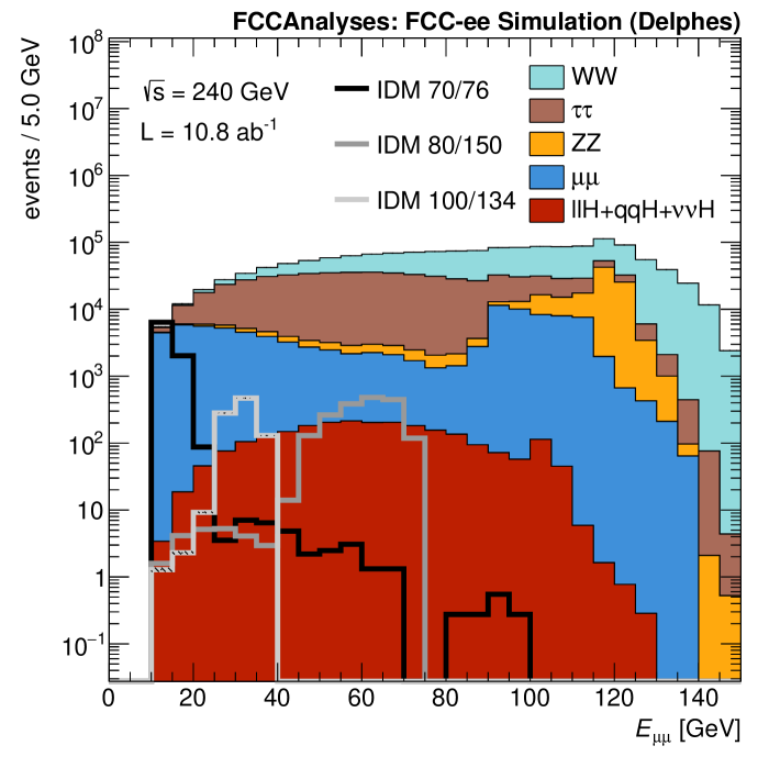
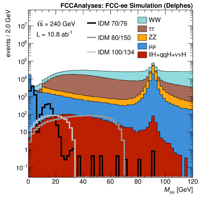
Figure 7: Distribution of the dimuon pair energy $E_{\mu\mu}$ (left) and invariant mass $M_{\mu\mu}$ (right) for $\sqrt{s}=$240 GeV, for the SM backgrounds and several selected signal mass points for the scenario S1. The signal mass points are labeled by IDM $M_{H}$/$M_{A}$ with masses given in GeV.

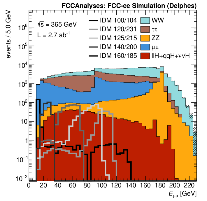
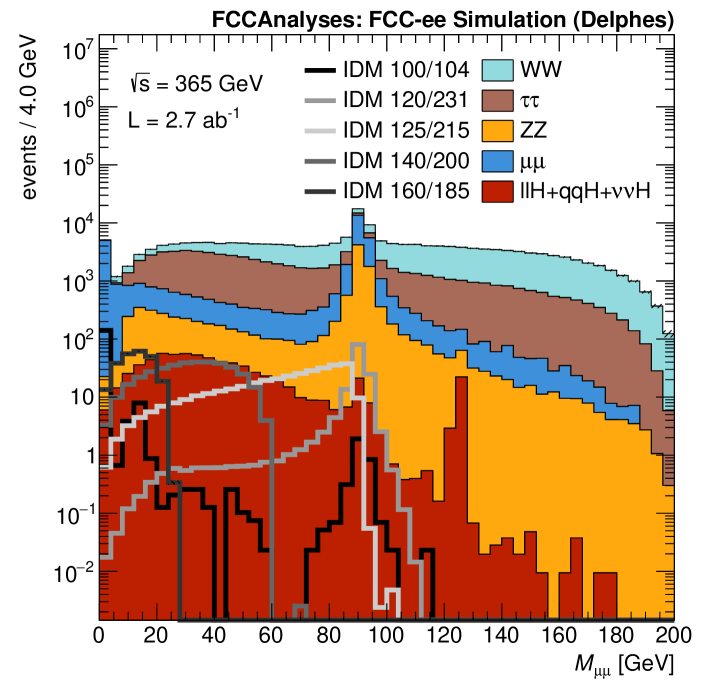
Figure 8: Distribution of the dimuon pair energy $E_{\mu\mu}$ (left) and invariant mass $M_{\mu\mu}$ (right) for $\sqrt{s}=$365 GeV, for the SM backgrounds and several selected signal mass points for the scenario S1. The signal mass points are labeled by IDM $M_{H}$/$M_{A}$ with masses given in GeV.

The pNN is implemented in PyTorch [48], and contains four sequential feed-forward layers each with 250 units and a ReLU activation function, totaling roughly 200,000 learnable parameters. The last three layers are preceded by a dropout layer with a rate of $0.2$, and the network output is passed through a sigmoid function for binary classification. The loss function for the training of the model is a weighted binary cross-entropy loss function:

$$\text{Weighted BCE}=-\frac{1}{N}\sum_{i=0}^{N}w_{i}[y_{i}\log(\text{pred}_{i})+(1-y_{i})\log(1-\text{pred}_{i})]$$ (3)

where the sum is over the samples, $\text{pred}_{i}$ is the model prediction, $y_{i}=\{0,1\}$ is the sample label, and $w_{i}$ is the sample weight. This is trained with the Adam optimiser with a learning rate of $0.0001$.

Each MC sample is split into three datasets: training, validation and test with fractions of the total dataset being 50%, 20% and 30%, respectively. The training set is used to train the model, and the validation set is used to measure the performance of the model during training. Finally, the model’s performance is evaluated using the test set.

Before training, events are re-weighted such that the sum of the signal weights equals the sum of the background weights. Moreover, the signals are re-weighted such that the sum of weights are equal for all IDM mass points to ensure that the training is not skewed towards certain signal points.

A single network is trained on both channels, $ee$ and $\mu\mu$, and all features that are passed to the pNN are standardised such that their mean is 0 and their standard deviation is 1. Training is conducted for 100 epochs, with early stopping if the validation loss does not decrease after 20 epochs. Finally, the model with the lowest validation loss is taken as the final model. No overfitting between the training, validation and test sets is found.

The pNN can smoothly interpolate to mass points not trained on when applied to the background samples. The signal distributions at intermediate points are found using cubic spline interpolation. This involves a shape parameter $\varepsilon$ that is determined by minimising the leave-one-out cross-validation error [49]. The interpolation capability of the setup was checked for several points of the parameter space, by comparing the results when those points are included or not in the training of the model. The pNN results were also compared with a simple implementation of a boosted decision tree using the same input features inside the TMVA framework [50], and comparable results were obtained on the individual IDM BPs.

The pNN distribution is shown for several representative signal mass points in Fig. 9 and 10 for $\sqrt{s}=$240 and 365 GeV, respectively. The top row shows the full distribution whilst the bottom row shows the distribution above 0.9 which is used for extracting the results in the next section.

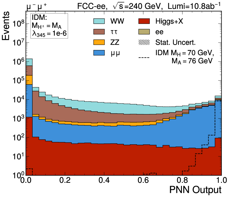
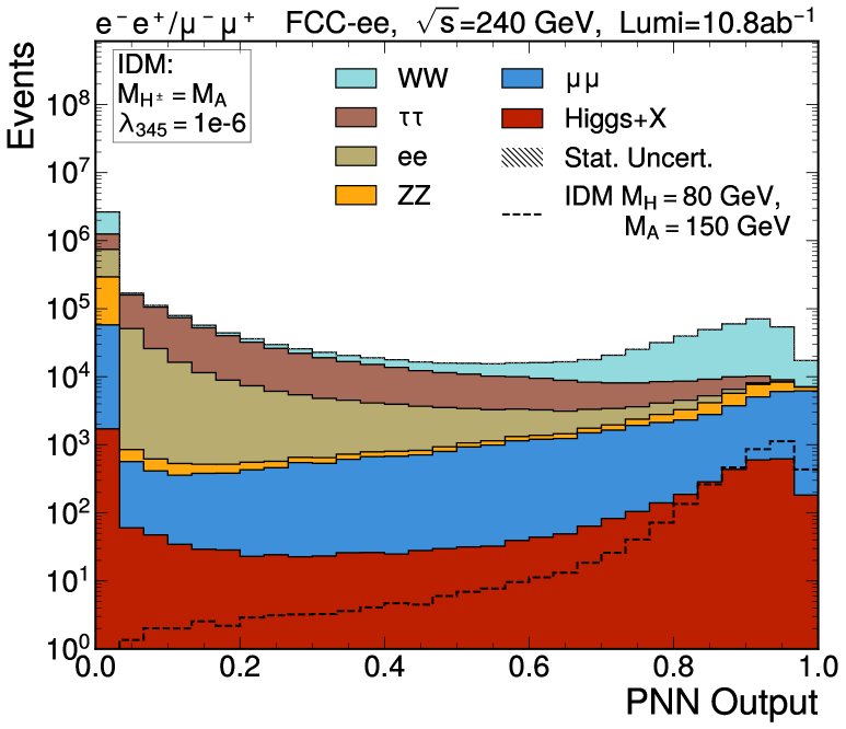
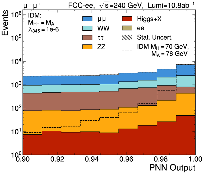
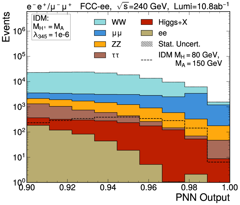
Figure 9: Output discriminator of the pNN for several signal points for $\sqrt{s}=$240 GeV samples summing $ee$ and $\mu\mu$ contributions if $M_{A}-M_{H}$$>30$ GeV, only $\mu\mu$ elsewhere. Top: full-range distribution, bottom: selection defining the signal region for the extraction of the results.

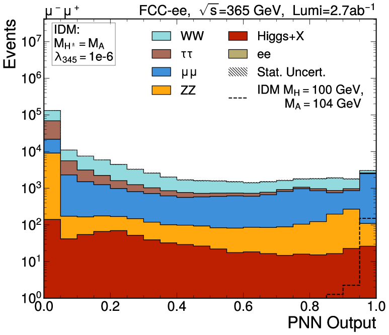
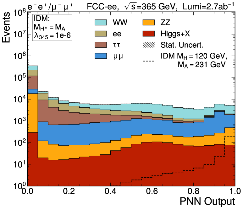
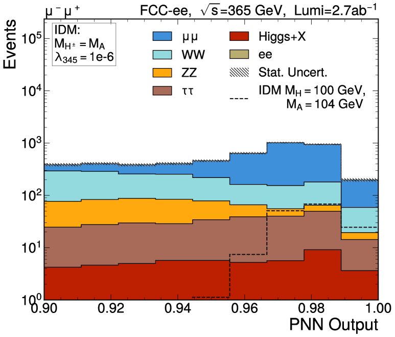
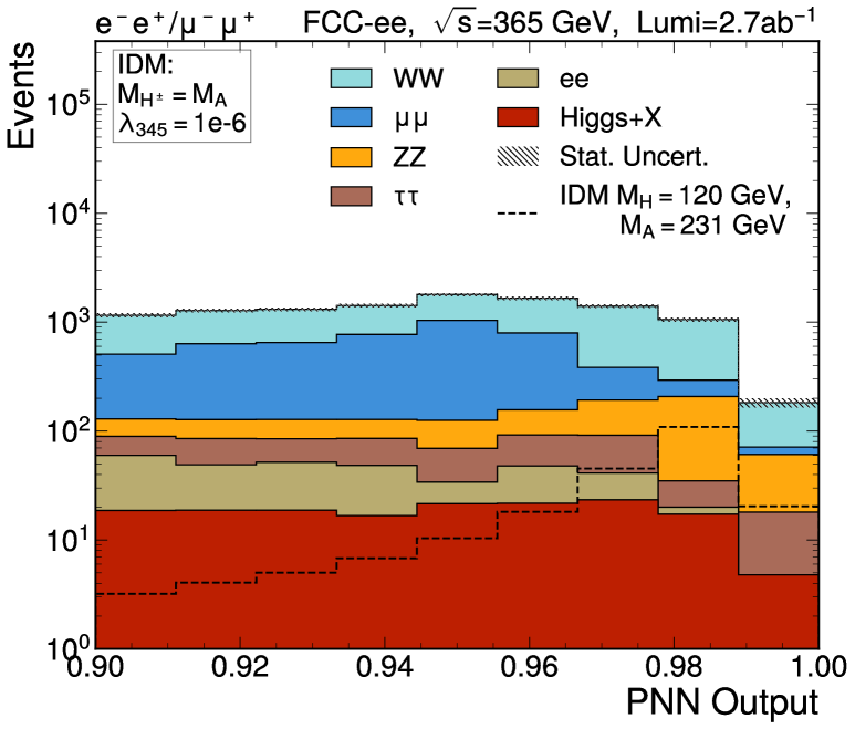
Figure 10: Output discriminator of the pNN for several signal points for $\sqrt{s}=$365 GeV samples summing $ee$ and $\mu\mu$ contributions if $M_{A}-M_{H}$$>30$ GeV, only $\mu\mu$ elsewhere. Top: full-range distribution, bottom: selection defining the signal region for the extraction of the results.

7 Results

A maximum likelihood fit of the pNN output above 0.9 is performed using the CMS Combine package [51]. A 95% confidence-level (CL) upper limit is derived using the asymptotic approximation [52]. A single source of uncertainties is included as nuisance parameters: the MC statistical uncertainties [53]. Future work should also include systematic uncertainties as additional nuisance parameters.

The $ee$ and $\mu\mu$ channels are fitted simultaneously. As the inclusive $ee$ production was simulated only for $M_{ee}>30$ GeV, the two final states $ee$ and $\mu\mu$ are combined for $M_{A}-M_{H}$$>30$ GeV, below which only the $\mu\mu$ result is shown.

The 95% CL exclusion region obtained is shown in Fig. 11 (left) in the $M_{A}-M_{H}$ vs $M_{H}$ plane, for $\sqrt{s}=$240 GeV, for the total integrated luminosity of 10.8 ab^-1. The three different scenarios defined in section 2 are shown as separate lines, well within the $\pm 1\sigma$ contour shown in green for scenario S1, including only the statistical uncertainties. The kinematic limit for on-shell production is highlighted by the dashed line. With the full luminosity of 10.8 ab^-1, almost the entire parameter space can be excluded at 95% CL, reaching $M_{H}$$=110$ GeV.

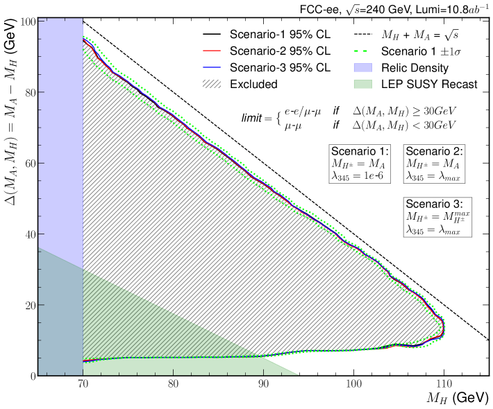
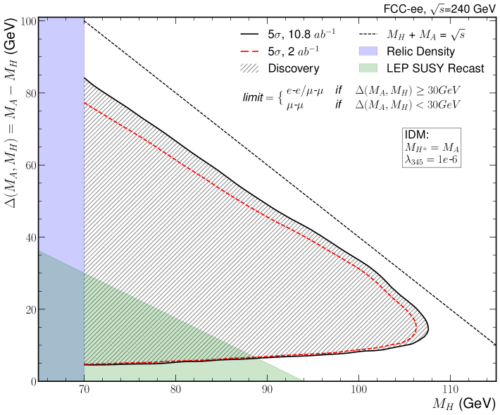
Figure 11: 95% CL expected exclusion (left) and $>5$-sigma discovery region (right) in the $M_{A}-M_{H}$ vs $M_{H}$ plane, for $\sqrt{s}=$240 GeV with total integrated luminosities of 10.8 and 2 ab^-1.

The $>5$-sigma discovery region is shown in Fig. 11 (right) for $\sqrt{s}=$240 GeV, in the scenario S1, for the total integrated luminosity of 10.8 ab^-1 and 2 ab^-1. The regions excluded by relic density constraints and LEP SUSY recast (see section 2) are overlayed. The discovery reach extends to $M_{H}$$=108\,\text{G\text{eV}}$ for $M_{A}-M_{H}$$=15$ GeV, for the nominal FCC luminosity scenario.

The 95% CL limit (left) and $>5$-sigma discovery (right) regions are shown in Fig. 12 for $\sqrt{s}=$365 GeV, for the total integrated luminosity of 2.7 ab^-1. The regions excluded by relic density constraints and LEP SUSY recast are overlayed. As for $\sqrt{s}=$240 GeV, the three different scenarios defined in section 2 are shown as separate lines and give results within the $\pm 1\sigma$ contour shown in green for scenario S1, including only the statistical uncertainties. The wedge in the distribution observed for a mass splitting around the on-shell Z boson mass is due to reduced sensitivity from reduced discrimination against background. The 95% CL excluded region reaches $M_{H}$$=165$ GeV. The discovery reach extends to $M_{H}$$=157$ GeV for $M_{A}-M_{H}$$=15$ GeV for the nominal FCC luminosity scenario, and is also shown in Fig. 12 right for a scenario with ten times less luminosity.

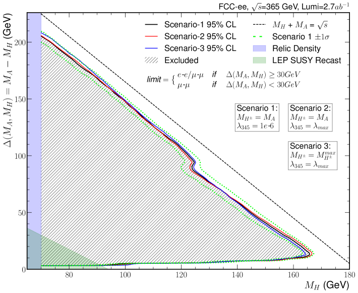
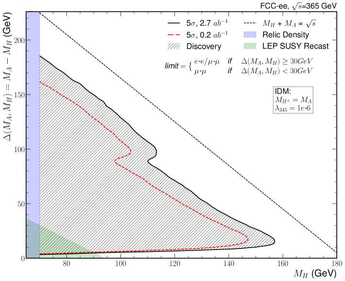
Figure 12: 95%CL limit (left) and $>5$-sigma discovery contour (right) in the $M_{A}-M_{H}$ vs $M_{H}$ plane, for $\sqrt{s}=$365 GeV with a total integrated luminosity of 2.7 ab^-1.

8 Conclusion

The Inert Doublet Model predicts additional scalars which couple only to bosons. The lighest neutral scalar, $H$, is also stable and provides an adequate dark matter candidate. The pair production of such new scalars is investigated in a final state containing two electrons or two muons, with $e^{+}e^{-}$ collisions at $\sqrt{s}=$240 and 365 GeV, in the context of the future circular collider at CERN, FCC-ee. With a total integrated luminosity of 10.8 (2.7)  ab^-1for $\sqrt{s}=$240 (365) GeV, almost the entire parameter space available in the $M_{A}-M_{H}$ vs $M_{H}$ plane is expected to be excluded at 95% CL, reaching up to $M_{H}$$=110\,(165)$ GeV, after using a parametric neural network trained to discriminate the different signal mass points against the backgrounds. The discovery reach is also explored and covers again almost the entire kinematic phase space available at $\sqrt{s}=$240 (365) GeV reaching $M_{H}$$=108\,(157)\,\text{G\text{eV}}$ for $M_{A}-M_{H}$$=15$ GeV.

References

References

- [1] S. Navas “Review of particle physics” In Phys. Rev. D 110.3, 2024, pp. 030001 DOI: 10.1103/PhysRevD.110.030001
- [2] Nilendra G. Deshpande and Ernest Ma “Pattern of Symmetry Breaking with Two Higgs Doublets” In Phys. Rev. D 18, 1978, pp. 2574 DOI: 10.1103/PhysRevD.18.2574
- [3] Riccardo Barbieri, Lawrence J. Hall and Vyacheslav S. Rychkov “Improved naturalness with a heavy Higgs: An Alternative road to LHC physics” In Phys. Rev. D 74, 2006, pp. 015007 DOI: 10.1103/PhysRevD.74.015007
- [4] Qing-Hong Cao, Ernest Ma and G. Rajasekaran “Observing the Dark Scalar Doublet and its Impact on the Standard-Model Higgs Boson at Colliders” In Phys. Rev. D 76, 2007, pp. 095011 DOI: 10.1103/PhysRevD.76.095011
- [5] Agnieszka Ilnicka, Maria Krawczyk and Tania Robens “Inert doublet model in light of LHC Run I and astrophysical data” In Physical Review D 93.5 American Physical Society (APS), 2016 DOI: 10.1103/physrevd.93.055026
- [6] Jan Kalinowski, Tania Robens, Dorota SokoÅowska and Aleksander Filip Åżarnecki “IDM Benchmarks for the LHC and Future Colliders” In Symmetry 13.6 MDPI AG, 2021, pp. 991 DOI: 10.3390/sym13060991
- [7] Daniel Dercks and Tania Robens “Constraining the Inert Doublet Model using Vector Boson Fusion” In Eur. Phys. J. C 79.11, 2019, pp. 924 DOI: 10.1140/epjc/s10052-019-7436-6
- [8] A. Abada “FCC-ee: The Lepton Collider: Future Circular Collider Conceptual Design Report Volume 2” In Eur. Phys. J. ST 228.2, 2019, pp. 261–623 DOI: 10.1140/epjst/e2019-900045-4
- [9] Alain Blondel and Patrick Janot “FCC-ee overview: new opportunities create new challenges” In Eur. Phys. J. Plus 137.1, 2022, pp. 92 DOI: 10.1140/epjp/s13360-021-02154-9
- [10] I. Agapov “Future Circular Lepton Collider FCC-ee: Overview and Status” In Snowmass 2021, 2022 arXiv:2203.08310 [physics.acc-ph]
- [11] Jan Kalinowski, Tania Robens, Dorota Sokolowska and Aleksander Filip Zarnecki “IDM Benchmarks for the LHC and Future Colliders” In Symmetry 13.6, 2021, pp. 991 DOI: 10.3390/sym13060991
- [12] A. Belyaev et al. “Advancing LHC probes of dark matter from the inert two-Higgs-doublet model with the monojet signal” In Phys. Rev. D 99.1, 2019, pp. 015011 DOI: 10.1103/PhysRevD.99.015011
- [13] Alexander Belyaev et al. “Anatomy of the Inert Two Higgs Doublet Model in the light of the LHC and non-LHC Dark Matter Searches” In Phys. Rev. D 97.3, 2018, pp. 035011 DOI: 10.1103/PhysRevD.97.035011
- [14] Agnieszka Ilnicka, Maria Krawczyk and Tania Robens “Inert Doublet Model in light of LHC Run I and astrophysical data” In Phys. Rev. D 93.5, 2016, pp. 055026 DOI: 10.1103/PhysRevD.93.055026
- [15] Agnieszka Ilnicka, Tania Robens and Tim Stefaniak “Constraining Extended Scalar Sectors at the LHC and beyond” In Mod. Phys. Lett. A 33.10n11, 2018, pp. 1830007 DOI: 10.1142/S0217732318300070
- [16] Jan Kalinowski et al. “Benchmarking the Inert Doublet Model for colliders” In JHEP 12, 2018, pp. 081 DOI: 10.1007/JHEP12(2018)081
- [17] Johannes Braathen, Martin Gabelmann, Tania Robens and Panagiotis Stylianou “Probing the Inert Doublet Model via Vector-Boson Fusion at a Muon Collider”, 2024 arXiv:2411.13729 [hep-ph]
- [18] David Eriksson, Johan Rathsman and Oscar Stal “2HDMC: Two-Higgs-Doublet Model Calculator Physics and Manual” In Comput. Phys. Commun. 181, 2010, pp. 189–205 DOI: 10.1016/j.cpc.2009.09.011
- [19] David Eriksson, Johan Rathsman and Oscar Stal “2HDMC: Two-Higgs-doublet model calculator” In Comput. Phys. Commun. 181, 2010, pp. 833–834 DOI: 10.1016/j.cpc.2009.12.016
- [20] Guido Altarelli and Riccardo Barbieri “Vacuum polarization effects of new physics on electroweak processes” In Phys. Lett. B 253, 1991, pp. 161–167 DOI: 10.1016/0370-2693(91)91378-9
- [21] Michael E. Peskin and Tatsu Takeuchi “A New constraint on a strongly interacting Higgs sector” In Phys. Rev. Lett. 65, 1990, pp. 964–967 DOI: 10.1103/PhysRevLett.65.964
- [22] Michael E. Peskin and Tatsu Takeuchi “Estimation of oblique electroweak corrections” In Phys. Rev. D 46, 1992, pp. 381–409 DOI: 10.1103/PhysRevD.46.381
- [23] I. Maksymyk, C.. Burgess and David London “Beyond S, T and U” In Phys. Rev. D 50, 1994, pp. 529–535 DOI: 10.1103/PhysRevD.50.529
- [24] I.. Ginzburg, K.. Kanishev, M. Krawczyk and D. Sokolowska “Evolution of Universe to the present inert phase” In Phys. Rev. D 82, 2010, pp. 123533 DOI: 10.1103/PhysRevD.82.123533
- [25] Georges Aad “Combination of searches for invisible decays of the Higgs boson using 139 fb1 of proton-proton collision data at s=13 TeV collected with the ATLAS experiment” In Phys. Lett. B 842, 2023, pp. 137963 DOI: 10.1016/j.physletb.2023.137963
- [26] Geneviève Bélanger et al. “micrOMEGAs5.0 : Freeze-in” In Comput. Phys. Commun. 231, 2018, pp. 173–186 DOI: 10.1016/j.cpc.2018.04.027
- [27] N. Aghanim “Planck 2018 results. VI. Cosmological parameters” [Erratum: Astron.Astrophys. 652, C4 (2021)] In Astron. Astrophys. 641, 2020, pp. A6 DOI: 10.1051/0004-6361/201833910
- [28] J. Aalbers “Dark Matter Search Results from 4.2 Tonne-Years of Exposure of the LUX-ZEPLIN (LZ) Experiment”, 2024 arXiv:2410.17036 [hep-ex]
- [29] Erik Lundstrom, Michael Gustafsson and Joakim Edsjo “The Inert Doublet Model and LEP II Limits” In Phys. Rev. D 79, 2009, pp. 035013 DOI: 10.1103/PhysRevD.79.035013
- [30] J. Alwall et al. “The automated computation of tree-level and next-to-leading order differential cross sections, and their matching to parton shower simulations” In JHEP 07, 2014, pp. 079 DOI: 10.1007/JHEP07(2014)079
- [31] Torbjörn Sjöstrand et al. “An introduction to PYTHIA 8.2” In Comput. Phys. Commun. 191, 2015, pp. 159–177 DOI: 10.1016/j.cpc.2015.01.024
- [32] Celine Degrande et al. “UFO - The Universal FeynRules Output” In Comput. Phys. Commun. 183, 2012, pp. 1201–1214 DOI: 10.1016/j.cpc.2012.01.022
- [33] A. Goudelis, B. Herrmann and O. Stål “Dark matter in the Inert Doublet Model after the discovery of a Higgs-like boson at the LHC” In JHEP 09, 2013, pp. 106 DOI: 10.1007/JHEP09(2013)106
- [34] The FCC Collaboration https://fcc-physics-events.web.cern.ch/fcc-ee/delphes/winter2023/idea/
- [35] Christian Bierlich “A comprehensive guide to the physics and usage of PYTHIA 8.3” In SciPost Phys. Codeb. 2022, 2022, pp. 8 DOI: 10.21468/SciPostPhysCodeb.8
- [36] Wolfgang Kilian, Thorsten Ohl and Jurgen Reuter “WHIZARD: Simulating Multi-Particle Processes at LHC and ILC” In Eur. Phys. J. C 71, 2011, pp. 1742 DOI: 10.1140/epjc/s10052-011-1742-y
- [37] Torbjorn Sjostrand, Stephen Mrenna and Peter Z. Skands “PYTHIA 6.4 Physics and Manual” In JHEP 05, 2006, pp. 026 DOI: 10.1088/1126-6708/2006/05/026
- [38] Patrick Janot, Christophe Grojean, Frank Zimmermann and Michael Benedikt “Integrated Luminosities and Sequence of Events for the FCC Feasibility Study Report”, 2024 DOI: 10.17181/nfs96-89q08
- [39] J. Favereau et al. “DELPHES 3, A modular framework for fast simulation of a generic collider experiment” In JHEP 02, 2014, pp. 057 DOI: 10.1007/JHEP02(2014)057
- [40] Giovanni F. Tassielli “A proposal of a drift chamber for the IDEA experiment for a future collider” In PoS ICHEP2020, 2021, pp. 877 DOI: 10.22323/1.390.0877
- [41] Gerardo Ganis, Clément Helsens and Valentin Völkl “Key4hep, a framework for future HEP experiments and its use in FCC” In Eur. Phys. J. Plus 137.1, 2022, pp. 149 DOI: 10.1140/epjp/s13360-021-02213-1
- [42] The FCC Collaboration https://github.com/HEP-FCC/FCCAnalyses
- [43] Matteo Cacciari, Gavin P. Salam and Gregory Soyez “FastJet User Manual” In Eur. Phys. J. C 72, 2012, pp. 1896 DOI: 10.1140/epjc/s10052-012-1896-2
- [44] Jan Kalinowski et al. “Exploring Inert Scalars at CLIC” In JHEP 07, 2019, pp. 053 DOI: 10.1007/JHEP07(2019)053
- [45] Aleksander Filip Zarnecki et al. “Searching Inert Scalars at Future e+e- Colliders” In International Workshop on Future Linear Colliders, 2020 arXiv:2002.11716 [hep-ph]
- [46] Pierre Baldi et al. “Parameterized neural networks for high-energy physics” In Eur. Phys. J. C 76.5, 2016, pp. 235 DOI: 10.1140/epjc/s10052-016-4099-4
- [47] Luca Anzalone, Tommaso Diotalevi and Daniele Bonacorsi “Improving Parametric Neural Networks for High-Energy Physics (and Beyond)”, 2022 DOI: 10.1088/2632-2153/ac917c
- [48] Adam Paszke et al. “PyTorch: An Imperative Style, High-Performance Deep Learning Library”, 2019 arXiv:1912.01703 [cs.LG]
- [49] Samuel Rippa “An algorithm for selecting a good value for the parameter c in radial basis function interpolation” In Advances in Computational Mathematics 11, 1999, pp. 193–210 URL: https://api.semanticscholar.org/CorpusID:3330803
- [50] A. Hoecker et al. “TMVA - Toolkit for Multivariate Data Analysis”, 2009 arXiv: https://arxiv.org/abs/physics/0703039
- [51] Aram Hayrapetyan “The CMS Statistical Analysis and Combination Tool: Combine” In Comput. Softw. Big Sci. 8.1, 2024, pp. 19 DOI: 10.1007/s41781-024-00121-4
- [52] Glen Cowan, Kyle Cranmer, Eilam Gross and Ofer Vitells “Asymptotic formulae for likelihood-based tests of new physics” [Erratum: Eur.Phys.J.C 73, 2501 (2013)] In Eur. Phys. J. C 71, 2011, pp. 1554 DOI: 10.1140/epjc/s10052-011-1554-0
- [53] J.. Conway “Incorporating Nuisance Parameters in Likelihoods for Multisource Spectra” In PHYSTAT 2011, 2011, pp. 115–120 DOI: 10.5170/CERN-2011-006.115