Towards a General-Purpose Zero-Shot Synthetic Low-Light Image and Video Pipeline

Abstract

Low-light conditions pose significant challenges for both human and machine annotation. This in turn has led to a lack of research into machine understanding for low-light images and (in particular) videos. A common approach is to apply annotations obtained from high quality datasets to synthetically created low light versions. In addition, these approaches are often limited through the use of unrealistic noise models. In this paper, we propose a new Degradation Estimation Network (DEN), which synthetically generates realistic standard RGB (sRGB) noise without the requirement for camera metadata. This is achieved by estimating the parameters of physics-informed noise distributions, trained in a self-supervised manner. This zero-shot approach allows our method to generate synthetic noisy content with a diverse range of realistic noise characteristics, unlike other methods which focus on recreating the noise characteristics of the training data. We evaluate our proposed synthetic pipeline using various methods trained on its synthetic data for typical low-light tasks including synthetic noise replication, video enhancement, and object detection, showing improvements of up to 24% KLD, 21% LPIPS, and 62% AP_50-95, respectively.

1 Introduction

The performance of computer vision methods for various image and video processing tasks (e.g. classification, action recognition, object detection, object tracking, instance segmentation, etc.) has advanced significantly in recent years. This is due primarily to advances in deep learning methods and increased computational power, allowing deeper and more complex networks to be trained. The demand for video-based research is evidenced by the numerous international challenges in recent years  [1, 2, 3, 4, 5, 6, 7]. This has, in turn, enabled many practical applications including autonomous driving, digital surveillance, augmented/virtual reality (AR/VR), media production, and entertainment.

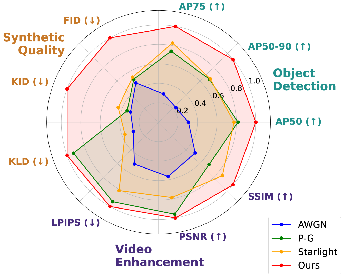
Figure 1: Comparison of our proposed method with existing synthetic noise pipelines, where our model outperforms these methods across numerous benchmarks. Results are taken from Table I and normalized for visualization. For metrics where lower is better, indicated by $\downarrow$, the results are inverted.

Despite these dramatic advances, research on processing videos captured under low-light conditions remains underdeveloped. Low light acquisition introduces numerous degradations such as low-contrast and motion blur, alongside sensor noise. All of these impact the performance of algorithms trained on normal-light data [8]. A further challenge is the lack of paired data, which is difficult to annotate accurately under low-light conditions without clear ground truth. As a result, only a limited number of datasets are available that offer adequate annotations for low-light video perception tasks [9, 10, 11, 12].

To overcome this, a common approach is to first apply low-light video enhancement (LLVE) methods [13, 14, 15, 16] before performing the desired downstream task. This enables models trained on normal-light conditions to process the video without having been trained specifically on low-light. Low-light enhancement is, however, an ill-posed problem, where a single low-light input could be mapped to multiple potential outputs. This may introduce greater variability into the system, making it more difficult to solve a downstream task with a single solution. Moreover, adding extra pre-processing steps increases computational complexity, especially for deep-learning-based methods, thereby limiting real-time applications. In addition, imperfect pre-processing of input data may produce artifacts that deteriorate the performance of downstream models  [17, 18].

An alternative approach is to generate synthetic data for training and evaluating the models. Mimicking real low-light conditions in this way removes the need to source suitable low-light datasets with the appropriate annotations; an existing clean dataset with annotations can be used instead. Although there are numerous pipelines available for creating synthetic low-light images and videos, each comes with limitations. Simpler pipelines often employ physics-informed distributions, which require manual selection of appropriate noise parameters  [19, 20] and fail to replicate sRGB-specific noise characteristics arising from in-camera processing pipelines. More complex pipelines may be tailored to specific types of noise, which significantly restricts their applications, or they may require camera-specific information that is not available in most publicly accessible datasets for downstream tasks.

In this context, we introduce a novel, general-purpose, zero-shot framework to address the limitations present in existing synthetic data pipelines. Our approach generates synthetic data with diverse, realistic noise characteristics, suitable for training models on new, noise-specific tasks. Crucially, our model operates without requiring training on individual datasets as it functions purely through inference on reference noisy data. This capability stems from our method of estimating a vector of noise parameters that maps to the corresponding physics-informed statistical distributions. By sampling from these distributions, our method can accurately replicate the noise characteristics found in any given reference input onto clean desired image or video data, enhancing the applicability and flexibility of the training data for noise-specific task models.

The main contributions are summarized as follows:

• The first general-purpose zero-shot synthetic low-light pipeline that outputs realistic low-light sRGB images and videos with the same noise characteristics as reference real low-light content. Our approach does not include any real low-light data during training, and allows desired noise characteristics to be applied onto any given input.

• Unlike the only existing zero-shot method proposed by [21], which is limited to Gaussian-distributed noise, our method offers a broad range of noise types and parameters, making it suitable for real-world applications.

• A novel Degradation Estimation Network (DEN) which can predict the parameters of physics-informed distributions to model the noise accurately onto low-light videos. This approach differs from existing works, which typically model output-specific noise based only on their specific training data.

• A novel self-supervised training strategy that exposes the DEN to a diverse distribution of noise parameters, enabling it to robustly learn and generalize across a wide range of noise characteristics.

The proposed method has been evaluated across various tasks, including synthetic noise replication, video enhancement, and object detection, demonstrating improvements of up to 24% KLD, 21% LPIPS, and 62% AP_50-95, respectively. Comparative analysis against established noise models, including Additive White Gaussian Noise (AWGN), Poisson-Gaussian noise (P-G) [19], and the Starlight noise generator [22], reveals our method’s superior performance, as shown in Fig. 1.

2 Related Work

2.1 RAW Noise Pipelines

RAW image data inherently contains various types of noise, often modeled using statistical distributions that reflect the physical processes of image capture. Many researchers make use of these physical phenomena to synthesize noisy data for training and analysis. The most commonly modeled noise type is read noise, which is typically modeled using a Gaussian distribution. Other forms of noise, such as shot noise, banding noise, or quantization noise, are also represented using appropriate statistical models. While these methods are capable of modeling many noise types using only statistics, they require manual parameter selection to ensure a realistic output. This is evidenced in work by Wei et al. [23], where meticulous experimentation was required to estimate the noise parameters for five different cameras.

More recently, there has been an increase in the use of deep-learning methods to synthesize realistic low-light images, without the need for parameter estimation [24, 25]. These methods are often ‘physics-guided’, allowing neural networks to learn the sampling of the relevant values for generating realistic low-light imagery. Cao et al. [24] developed a method that models a variety of different noise types, but it requires the availability of ISO information for the image. Meanwhile, Zhang et al. [25] proposed a more general-purpose pipeline, but solely focus on read and shot noise. Monakhova et al. [22] proposed a generative adversarial network (GAN) for synthesizing noisy RAW videos to train their denoiser. Similar to other pipelines, their method employs physics-guided noise, where the GAN initially samples from several statistical distributions with learned parameters for their dataset, followed by processing the video through a U-Net [26] to learn other complex noise types. However, their method requires re-training when applied to different cameras or datasets, highlighting a common limitation in the generalizability of current noise synthesis approaches.

2.2 sRGB Noise Pipelines

Many synthetic pipelines predominantly use the RAW format to model noise based on physics principles. However, sRGB images inherently exhibit additional degradation types which need to be considered. One of the main degradation types is spatially-correlated noise, which is often caused by compression algorithms. Due to the complex nature of noise types like this, limited research has been conducted for synthetic noisy sRGB pipelines. Deep learning approaches have been explored, but these usually require further information about the image, such as camera parameters and ISO settings. For example, Kousha et al. [27] synthesized noisy sRGB images by leveraging normalizing flows, a family of generative models which use invertible transformations to translate data from one domain to another. Their method includes a specific linear flow layer conditioned on the camera metadata and gain (ISO) to ensure accurate synthetic noisy images.

Fu et al. [28] introduced an alternative approach for generating noisy sRGB images that accounts for spatially-correlated noise without the need for ISO data of the captured image. They proposed a ‘gain estimation network’ that enables the model to autonomously synthesize noise without additional camera information. However, their method is still limited in terms of applications, as it is unable to generalize across different camera models, requiring re-training for each distinct camera.

2.3 Low-Light sRGB Pipelines

Existing pipelines for generating low-light images and videos often rely on simpler models that primarily capture common noise types such as read and shot noise, and primarily focus on modifying the brightness and contrast of the data. This approach generally lacks the sophistication required to replicate realistic noise conditions effectively.

Lv et al. [29] proposed a method for generating low-light images which mimics the image signal processing (ISP) pipeline in low-light photography. They first reduce the brightness of the images using a combination of linear and power transformations, before converting the images to a Bayer format. This synthetically creates a ‘RAW’ low-light image, where physics-informed noise types (i.e. read and shot noise) are applied, before converting back into sRGB format via demosaicing techniques. Cui et al. [30] also proposed a similar approach to simulating the ISP pipeline, but factor in further image transformations such as white balance and gamma correction to enhance realism.

For videos, Zhou et al. [31] proposed a synthetic low-light pipeline focusing on motion blur due to low-light conditions. Unlike the simpler brightness adjustment techniques, they use a modified version of Zero-DCE [13] to reduce the brightness of the image, instead of simple linear or power transformations. However, only Gaussian and Poisson noise distributions are present in their noise model.

3 Proposed Method

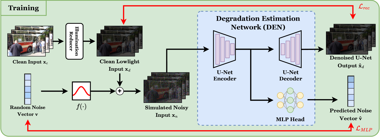
Figure 2: The outline for training with our proposed Degradation Estimation Network (DEN), including its architecture. The architecture of the DEN consists of a U-Net [26] combined with a Multi-Layer Perceptron (MLP) head after the encoder to estimate the noise vector $\hat{\mathbf{v}}$ with denoising guidance.

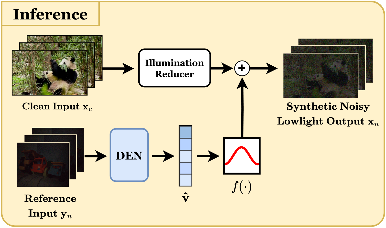
Figure 3: The process for inferencing the DEN. A real noisy video is passed into the model to obtain the noise vector $\hat{\mathbf{v}}$, which accurately describes the noise characteristics in the video. The vector is used to sample from the relevant distributions onto the clean inputs to synthetically generate low-light videos.

We propose a new zero-shot generic synthetic noise pipeline capable of generating realistic low-light videos that accurately replicates the noise characteristics observed in a given reference video. This pipeline is also applicable to images by simply reducing the temporal dimension to one. To allow for zero-shot capabilities and to ensure robustness across various camera settings and noise characteristics, we employ a self-supervised training strategy that involves the generation of images and videos with a large and representative range of noise characteristics. Our approach guarantees that our method adapts to diverse noise patterns typically seen across different camera systems or the same system with different settings. The training and inference processes are illustrated in Fig. 2, and Fig. 3, respectively.

In the training phase, our methodology begins by attenuating the brightness of clean input data using linear and power transformations, referred to as the ‘illumination reducer’ in Fig. 2. We set

$$\mathbf{x}_{d}=\alpha\mathbf{x}_{c}^{1/\gamma},$$ (1)

where $\mathbf{x}_{d}$ is the darkened image and $\mathbf{x}_{c}$ is the clean input image. The coefficients $\alpha$ and $\gamma$ are sampled from uniform distributions, empirically $\alpha\sim\mathcal{U}(0.05,0.3)$ and $\gamma\sim\mathcal{U}(0.1,1)$, to vary the intensity and gamma correction of the synthesized imagery respectively.

Following this darkening process, random values are selected for each noise type described in Section 3.1, and applied to the input data. Subsequently, we pass this video into our Degradation Estimation Network (DEN), which learns to estimate the vector of the parameters, referred to as the noise vector $\mathbf{v}$, from the distributions that the noise map is sampled from. Concurrently, the DEN is trained to perform denoising used for optimization ($\mathcal{L}_{rec}$ in Fig. 2), enhancing its ability to generalize across various noise conditions.

During the inference phase, real low-light images or videos serve as the reference inputs $\mathbf{y}_{n}$ to the DEN, which predicts the noise vector that most accurately represents the noise characteristics present in the reference video. The predicted noise vector is then used to simulate noise, effectively replicating the noise patterns found in the low-light conditions of the reference data.

The overall inference process can be summarized as

$$\begin{split}\mathbf{x}_{n}&=\mathbf{x}_{d}+f(\mathbf{\hat{v}}),\\ \mathbf{\hat{v}}&=\text{DEN}(\mathbf{y}_{n}),\end{split}$$ (2)

where $\mathbf{x}_{n}$ stands for the synthesized low-light image or video, and $\mathbf{y}_{n}$ is the reference videos with real noise. $\mathbf{\hat{v}}$ represents the estimated noise vector which contains the parameters for the noise distribution models, and $f(\cdot)$ is the noise simulation function comprised of various noise models.

Crucially, our method ultimately allows for the training of any model on any reference noise types. This process involves analyzing the input data to constrain the range of values for the random noise vector $\mathbf{v}$ used during inference of our method in the downstream model training. By doing so, the model in question can be specifically trained on targeted noise characteristics or specific downstream tasks, greatly enhancing its effectiveness.

3.1 Physics-Based Noise

In our framework, we focus on physics-based noise to accurately simulate realistic noise characteristics prevalent in low-light conditions. Five predominant noise types are modeled as follows.

Read noise and shot noise are typical in low-light imagery  [32, 33]. Read noise arises from electrical noise inherent in the signal readout process from the camera sensor. It is a combination of a variety of noise types that can generally be modeled using a Gaussian distribution [33]. Shot noise, on the other hand, results from the quantum nature of light. During image capture, some photons may not have reached the sensor, leading to image degradation. This type of noise is particularly more noticeable in low-light scenes where photon counts are low. This effect can be modeled using a Poisson distribution. To simulate both types of noise, we employ the heteroscedastic noise model proposed by Foi et al. [19], which approximates the Poisson distribution as zero-mean Gaussian. The heteroscedastic noise model is beneficial as it can approximate shot noise, a type of signal-dependent noise that is not inherently additive, to be treated in an additive manner. The heteroscedastic noise model is mathematically described for a video frame of height $H$, width $W$ and channels $C$ as

$$\mathbf{n}_{h}\sim\mathcal{N}(0,\sigma_{s}^{2}\mathbf{x}+\sigma_{r}^{2}),\quad\mathbf{n}_{h}\in\mathbb{R}^{C\times H\times W},$$ (3)

where $\mathbf{n}_{h}$, $\mathbf{x}$, $\sigma_{s}^{2}$, and $\sigma_{r}^{2}$ are the heteroscedastic noise, the clean image signal, the signal-dependent (shot noise) variance coefficient, and the signal-independent (read noise) variance, respectively.

Quantization noise arises during the process of converting the analog signal (with continuous values) into a digital signal (with discrete values). This conversion often introduces visual artifacts in the form of grainy or blocky images, which is especially noticeable in images with low bit depth. We model this using a uniform distribution

$$\mathbf{n}_{q}\sim\mathcal{U}(0,\lambda_{q}),\quad\mathbf{n}_{q}\in\mathbb{R}^{C\times H\times W},$$ (4)

where $\mathbf{n}_{q}$ is the quantization noise map, and $\lambda_{q}$ is the upper bound for the quantization noise interval.

Banding noise refers to the horizontal or vertical lines that become prominent at high ISO, commonly used in low-light photography and videography to capture content without the need for long shutter speeds (which causes motion blur). This type of noise is highly camera-specific. Banding noise, like vertical banding as outlined by Monakhova et al. [22], is modeled using a Gaussian distribution centered at zero, with the variability of band positions encapsulated by the standard deviation $\sigma_{b}$. The noise model is represented as

$$\mathbf{n}_{b}\sim\mathcal{N}(0,\sigma_{b}^{2}),\quad\mathbf{n}_{b}\in\mathbb{R}^{C\times 1\times W},$$ (5)

where $\mathbf{n}_{b}$ is the banding noise map. Additionally, we include temporal banding noise $\mathbf{n}_{b_{t}}$ (as described in [22]), where banding noise maintains consistency throughout the video, characterized by a standard deviation of $\sigma_{b_{t}}$ to model noise persistence over time.

Periodic noise appears as a repeating pattern, often caused by electrical interference during the image capturing process. It is characterized by regularly spaced artifacts such as stripes or grids. Periodic noise is distinct from banding noise due to its strictly periodic nature. Unlike random noise, periodic noise can be effectively identified in the frequency domain, where it exhibits as distinct peaks. We follow the periodic noise implementation described in [22], which is formulated by

$$\mathbf{n}_{p}[r,c]=\begin{cases}\mathcal{F}^{-1}(\mathbf{n}_{p_{1}}),&\text{if}\>\>c=0,\\ \mathcal{F}^{-1}(\mathbf{n}_{p_{2}}+\mathbf{n}_{p_{3}}i),&\text{if}\>\>c=W/4,\\ \mathcal{F}^{-1}(\mathbf{n}_{p_{2}}-\mathbf{n}_{p_{3}}i),&\text{if}\>\>c=3W/4,\\ 0,&\text{otherwise},\end{cases}$$ (6)

where $r$ and $c$ index the row and column of the image, respectively, and $\mathcal{F}^{-1}$ is the inverse Fourier transform. $\mathbf{n}_{p_{1}}$, $\mathbf{n}_{p_{2}}$ and $\mathbf{n}_{p_{3}}$ are random variables, each sampled from zero-mean Gaussian distributions with standard deviations $\sigma_{p_{1}}$, $\sigma_{p_{2}}$ and $\sigma_{p_{3}}$ respectively.

3.2 Degradation Estimation Network (DEN)

Our proposed DEN is designed to replicate the noise characteristics of a given reference low-light image or video $\mathbf{y}_{n}$. In practice, it is trained to predict a noise vector $\mathbf{\hat{v}}$ that configures the noise simulator $f(\cdot)$ with the appropriate parameters. Referring to Section 3.1, the DEN aims to predict the following parameters: $\sigma_{s}$, $\sigma_{r}$, $\lambda_{q}$, $\sigma_{b}$, $\sigma_{b_{t}}$, $\sigma_{p_{1}}$, $\sigma_{p_{2}}$ and $\sigma_{p_{3}}$.

The architecture of the DEN is built upon a U-Net framework [26], with an additional multi-layer perceptron (MLP) [34] head following the encoder. The MLP head is tasked with estimating the noise vector for simulating the noise in the reference data, whereas the decoder reconstructs the denoised version of the input video. The reasoning behind this design is to enable the encoder to effectively discriminate noise from the underlying image content, guiding the MLP head to precise noise vector predictions.

The DEN loss function comprises two components, $\mathcal{L}_{MLP}$ and $\mathcal{L}_{rec}$, to train the weights in both heads of the network. The loss function for the MLP head, $\mathcal{L}_{MLP}$, is calculated using the mean-squared error (MSE) between the predicted noise vector $\mathbf{\hat{v}}$ and the target noise vector $\mathbf{v}$, defined as

$$\mathcal{L}_{MLP}=\frac{1}{n}\sum_{i=1}^{n}(v_{i}-\hat{v}_{i})^{2},$$ (7)

where $n$ is the number of elements in vector $\mathbf{v}$, $v_{i}$ is the $i^{\text{th}}$ element in the input noise vector, and likewise, $\mathbf{\hat{v}}_{i}$ is the $i^{\text{th}}$ element in the predicted noise vector.

The second component, $L_{rec}$, is a reconstruction loss to train the decoder head to denoise the input, defined as

$$\mathcal{L}_{rec}=\frac{1}{n}\sum_{i=1}^{n}\lvert\mathbf{x}_{d}-\mathbf{\hat{x}}_{d}\rvert,$$ (8)

where $\mathbf{x}_{d}$ is the darkened clean input, and $\mathbf{\hat{x}_{d}}$ is the reconstructed denoised input. Adding the two losses together, we have

$$\mathcal{L}_{DEN}=\lambda_{1}\mathcal{L}_{MLP}+\lambda_{2}\mathcal{L}_{rec}$$ (9)

where $\lambda_{1}$ and $\lambda_{2}$ are the adjustable hyperparameters for each loss.

The denoising head employs the $\ell_{1}$ loss function due to its robustness to outliers, enhancing the stability of denoising operations. Conversely, for estimating the noise vector $\mathbf{v}$, we utilize the $\ell_{2}$ loss function, which penalizes larger deviations more heavily, ensuring that the estimated noise closely approximates actual noise characteristics observed in the data.

3.3 Noise Simulator $f(\cdot)$

The noise simulator function $f(\cdot)$ is designed to synthesize realistic noise maps present in images and videos by leveraging the physics-based noise models detailed in Section 3.1. This function takes a noise parameter vector $\mathbf{v}$, predicted by the DEN using the real noisy input. The vector $\mathbf{v}$ compiles the necessary parameters to control the intensity and characteristics of each noise type: $\mathbf{v}=[\sigma_{s},\sigma_{r},\lambda_{q},\sigma_{b},\sigma_{b_{t}},\sigma_{p_{1}},\sigma_{p_{2}},\sigma_{p_{3}}]$.

Most of the noise types used in this simulation are signal-independent and modeled as additive noise, while shot noise is signal-dependent and is typically applied onto the image. However, by adopting the heteroscedatic noise model [19], read-shot noise can be approximated as additive, allowing for easier calculations. As a result, the final simulated noise map is defined as the summation of all individual noise components, expressed as

$$f(\mathbf{v})=\mathbf{n}_{h}+\mathbf{n}_{q}+\mathbf{n}_{b}+\mathbf{n}_{b_{t}}+\mathbf{n}_{p},$$ (10)

where $\mathbf{n}_{h},\mathbf{n}_{q},\mathbf{n}_{b},\mathbf{n}_{b_{t}}$ and $\mathbf{n}_{p}$ represent the specific noise maps generated by sampling from their respective distributions or applying their defined procedures (as detailed in Equations 3-6) using the parameters contained within the input vector $\mathbf{v}$.

4 Experimental Results and Discussion

4.1 Implementation Details

We utilize the YouTube-VOS dataset [3] for training our network, which includes 3,471 videos representative of diverse real-world scenarios. It also features extensive variability in both object types and movement dynamics for greater generalizability. We train our method for 10 epochs with a batch size of 2 and 16 frames per video. We employ the Adam optimizer with a learning rate of 0.0002, $\beta_{1}$ of 0.5 and $\beta_{2}$ of 0.999. Weights $\lambda_{1}$ and $\lambda_{2}$ are both set to 1.

For performance benchmarking, we compare our framework against several noise models, including Additive White Gaussian Noise (AWGN), Poisson-Gaussian noise (P-G) as approximated by Foi et al. [19], and the Starlight noise generator proposed by Monakhova et al. [22]. The Starlight model is fully re-trained under identical settings as ours and adapted for processing sRGB videos instead of RAW inputs. The consistent training strategy ensures a fair comparison. Importantly, we do not compare our model against other sRGB deep-learning pipelines, such as [27, 28], as they require camera metadata, which would otherwise result in an unfair comparison, and this information is unknown in many real-world cases.

TABLE I: Quantitative Results of Synthetic Pipelines Across Multiple Experiments. The best performers are highlighted in bold, and the second best are underlined.

Method	Synthetic Quality			LLVE					Object Detection
	KLD$\downarrow$	FID$\downarrow$	KID$\downarrow$	PSNR$\uparrow$	SSIM$\uparrow$	LPIPS$\downarrow$	CLIP-IQA$\uparrow$	NIQE$\downarrow$	AP50-95(%)$\uparrow$	AP50(%)$\uparrow$	AP75(%)$\uparrow$
AWGN	0.458	258.635	0.450	29.716	0.849	0.165	0.205	6.234	18.474	20.328	19.812
P-G [19]	0.358	254.760	0.444	30.222	0.855	0.134	0.199	5.943	25.213	29.167	27.083
Starlight [22]	0.444	252.610	0.428	30.006	0.860	0.143	0.260	5.812	25.337	28.465	28.465
Ours	0.347	211.219	0.337	30.272	0.864	0.130	0.200	5.565	29.919	32.343	31.291

4.2 Synthetic Quality Assessment

For a quantitative analysis of the performance of each synthetic pipeline, we calculate the Kullback–Leibler divergence (KLD), Fréchet Inception Distance (FID) [35] and Kernel Inception Distance (KID) [36] between the real noise maps and the synthetic noise maps. KL divergence is a broadly-applied statistical measure for quantifying the distance between probability distributions, and therefore is a highly suitable metric for our assessment. FID and KID are two popular metrics used in image generation tasks for measuring the performance of generative models. FID measures the distance between two multivariate Gaussians fitted to feature representations of the input dataset against those of the target set. Unlike FID, KID does not assume a Gaussian distribution but instead uses Maximum Mean Discrepancy.

We use the SIDD-Small dataset [37] for evaluation as it covers a wide range of noise characteristics, which are influenced by various ISO levels, shutter speeds, illuminant temperatures, lighting conditions) across 5 different camera models. Moreover, the clean images are provided, allowing for the computation of real noise maps. The results, presented in Table I (under ‘Synthetic Quality’), demonstrate that our synthetic noise pipeline achieves the best results for all 3 metrics relative to the real noise, indicating a higher fidelity in noise replication. We would like to note that the FID scores are inflated, reflecting the metric’s strong bias with respect to sample size.

We also present visual comparisons of the results from each synthetic pipeline in Fig. 4 for qualitative analysis. Our method exhibits superior performance, adapting noise parameters dynamically to the noisy reference input. Subjectively, our results appear closer to the reference (noted as ‘Real’ in the figure) and do not overestimate noise like other methods. However, as shown in Fig. 4, there is evident noise reduction applied in the real noisy images, but our pipeline does not incorporate blur effects or other in-camera post-processing. These complex degradations will be addressed in our future work.

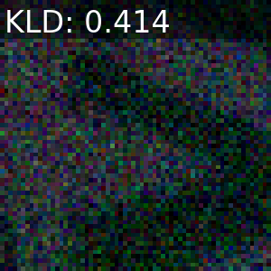
AWGN

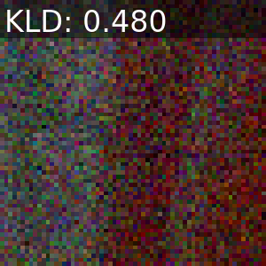
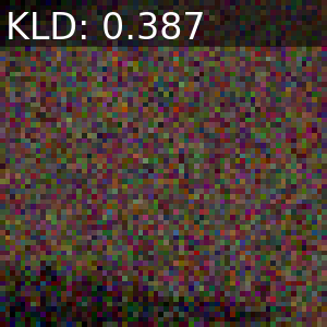
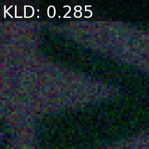
P-G [19]

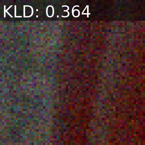
Starlight [22]

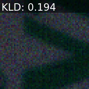
Ours

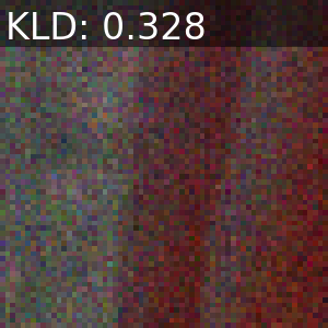
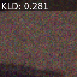
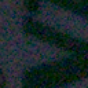
Real

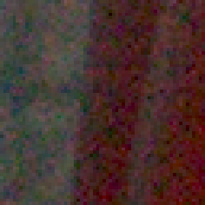
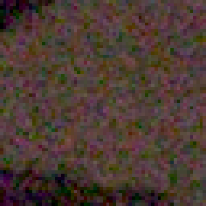
Figure 4: Visual comparison of different synthetic pipelines compared against the real low-light images from the SIDD-Small dataset [37]. The KL divergence for each synthetic image is also provided.

4.3 Low-Light Video Enhancement (LLVE)

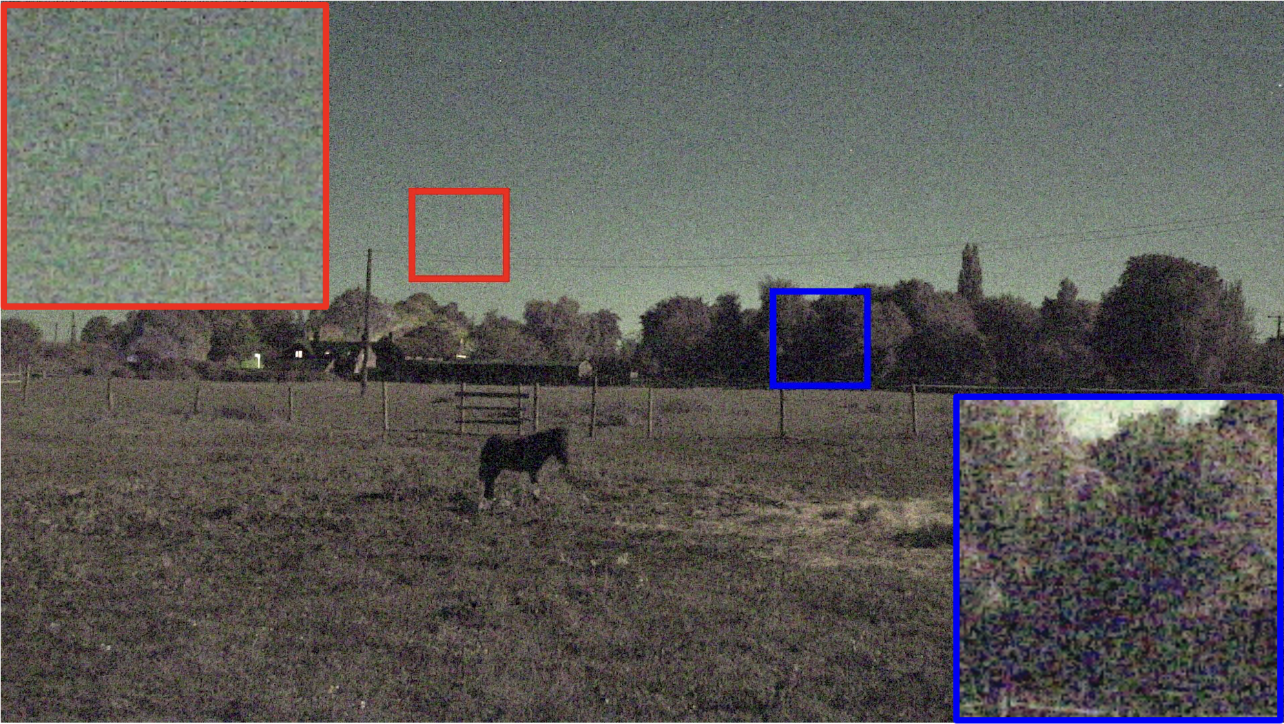
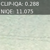
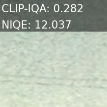
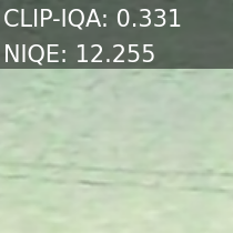
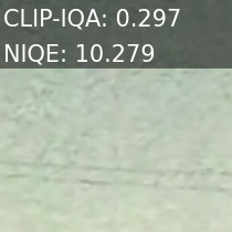
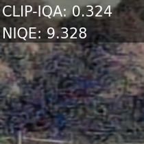
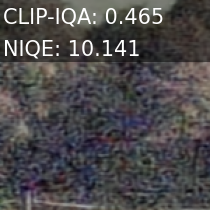
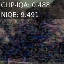
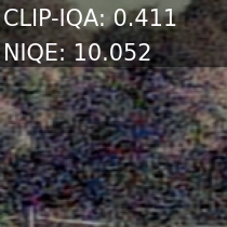
AWGN

P-G [19]

Starlight [22]

Ours

Figure 5: Qualitative comparison of the outputs of four BVI-Mamba [38] models trained with their respective noise pipelines on an extreme example of low-light noise. Simpler models are unable to capture the high degree of variability in the scene’s noise, while more sophisticated models such as Starlight and ours allow BVI-Mamba to learn to denoise more effectively.

We assess the performance of our noise simulator on low-light video enhancement through quantitative and qualitative analysis. Given that most low-light enhancement methods are proposed for images, and because there are fewer video-specific methods due to the increased computational costs, we select a pre-trained low-light video enhancement model BVI-Mamba [38], which reduces computational complexity by employing Visual State Space (VSS) blocks. The dataset used for pre-training is the BVI-RLV [38] dataset, which offers over 30K fully registered HD paired video frames in normal and dark conditions with predefined training and testing video sets.

We conduct testing using a real noisy low-light HD video, referred to as the ‘horse’ video, captured outdoors after sunset with a Canon ML-105 camera (Fig. 5 left). Our synthetic noise is generated using the DEN model, with this ‘horse’ video serving as $\mathbf{y}_{n}$. For training, synthetic noise from each pipeline is added to the BVI-RLV training set following Equation 1.

The first experiment analyzes how well the low-light enhancer can learn different noise characteristics. We independently apply the same synthetic noise from each pipeline to the BVI-RLV testing sets. The enhanced outputs are then compared with the clean, normal-light ground truths. Objective metrics including Peak Signal-to-Noise Ratio (PSNR), Structural Similarity Index Measure (SSIM), and perceptual similarity metrics like LPIPS [39], are used to evaluate the performance of four different pipelines. The quantitative results can be seen in Table I.

The second analysis evaluates how closely the noise simulators can replicate the characteristics of the ’horse’ video. We enhance this real video using models trained with various synthetic noises. As there is no ground truth available, we calculate no-reference metrics CLIP Image Quality Assessment (CLIP-IQA) [40] and Naturalness Image Quality Evaluator (NIQE) [41], for a quantitative comparison. Higher CLIP-IQA scores and lower NIQE scores indicate better perceptual quality. The prompts used for CLIP-IQA are ‘quality’, ‘brightness’, and ‘noisiness’. Visual comparisons are shown in Fig. 5. Models trained with synthetic noise from our pipeline achieve a better balance between perceptual quality and naturalness. In smooth, bright regions such as the sky, shown in the top row, our method achieves the best NIQE scores compared to all other pipelines. Although Starlight has the highest CLIP-IQA, it produces artifacts like color distortion. In textured, dark areas, such as the tree region shown in the bottom row, Starlight and P-G achieve better CLIP-IQA scores, suggesting they might be better at enhancing brightness or details in those regions. However, results trained on our pipeline still maintain competitive NIQE scores.

We further evaluate the impact of enhancement on object detection performance by using the pre-trained YOLOv11n model to detect a horse located in the middle of a scene. Importantly, this object was not detectable in the original noisy video due to the provided model being trained only on clean images. Post-enhancement results, depicted in Fig. 6, reveal that the YOLOv11n model successfully detects the horse in the output enhanced by BVI-Mamba trained on our synthetic data. In contrast, the horse is mislabeled when using the enhancer trained on Starlight data. When enhanced with AWGN data, the model erroneously predicts the presence of both a cow and a horse. Although the P-G data allows for successful horse detection, the confidence of the YOLOv11n model is notably lower compared to its performance with our synthetic data.

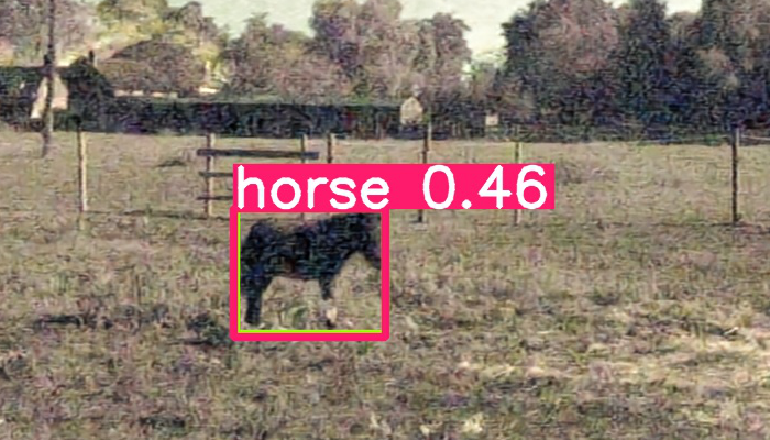
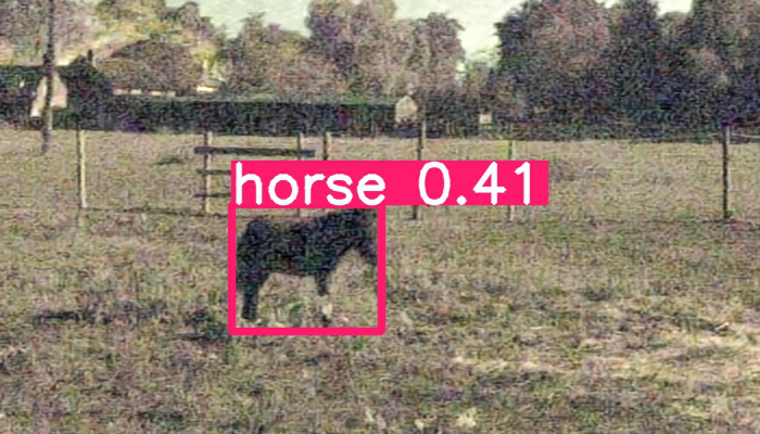
AWGN

P-G [19]

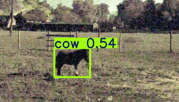
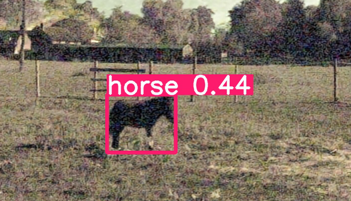
Starlight [22]

Ours

Figure 6: Qualitative comparison of the pre-trained YOLOv11n [42] on outputs of four BVI-Mamba models trained with their respective noise pipelines. The denoiser trained using our approach allows successful detection of a horse, while the model trained using Starlight results in the detection of a cow.

4.4 Object Detection

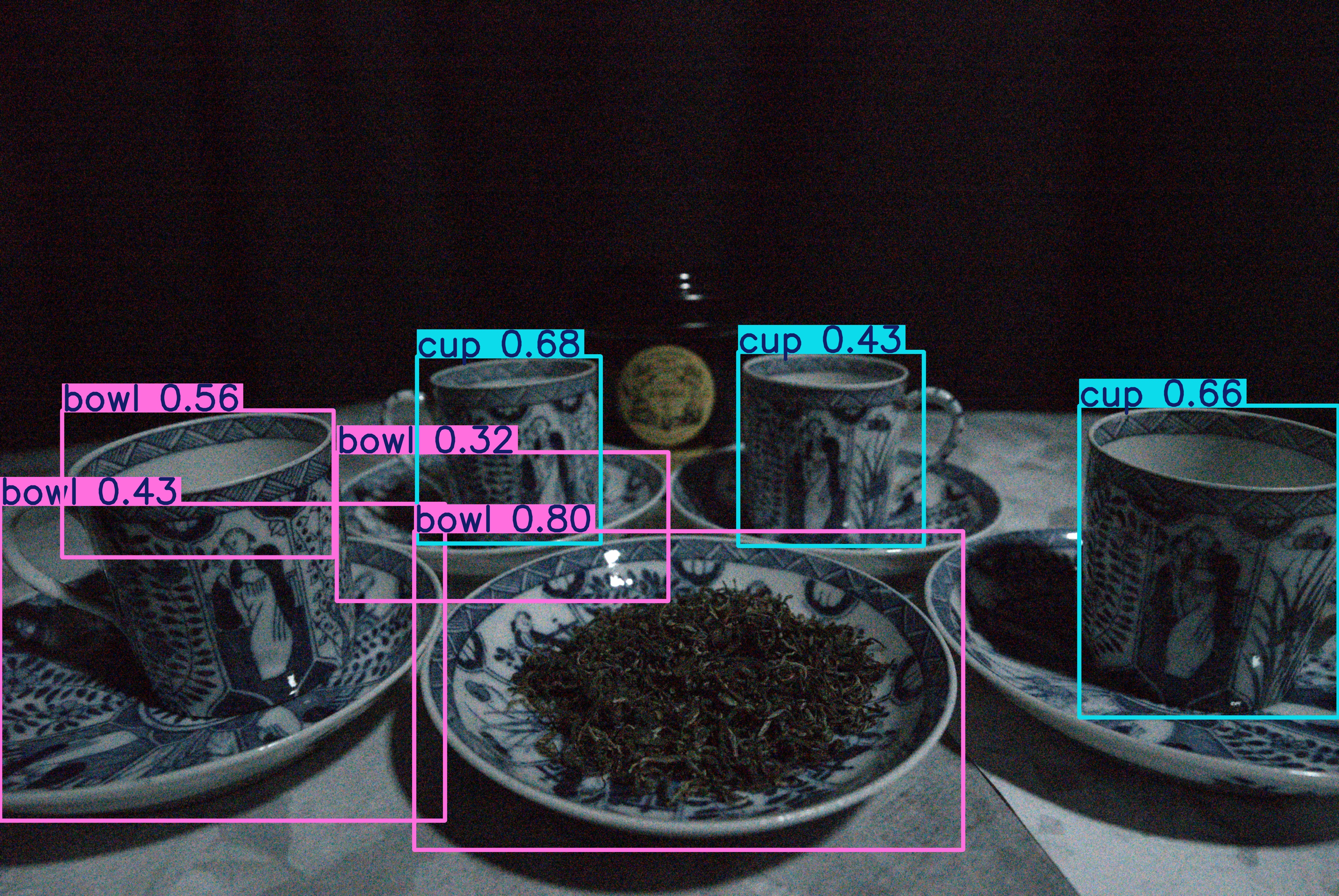
(a) Pre-trained YOLOv11n on noisy input.

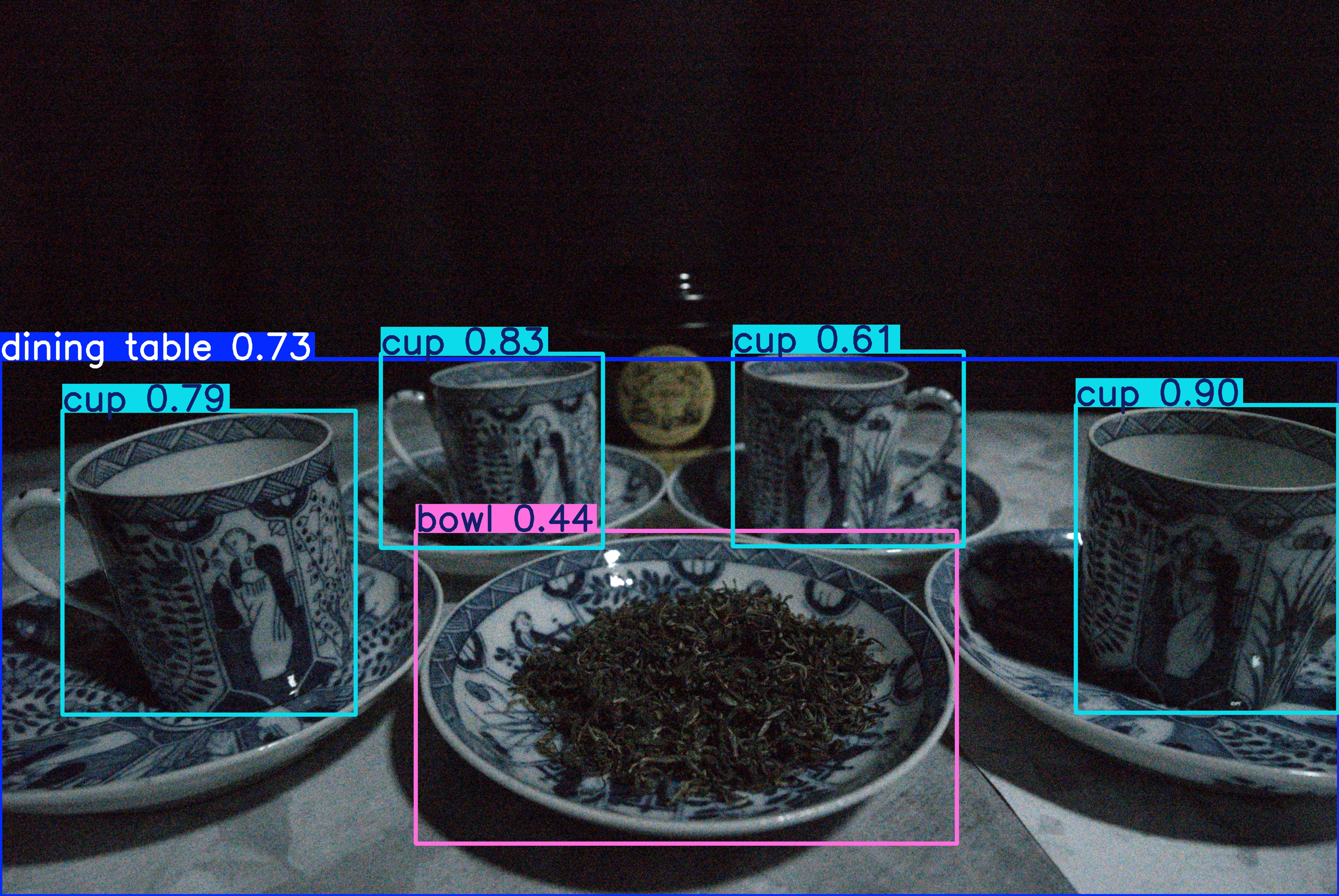
(b) Our YOLOv11n on noisy input.

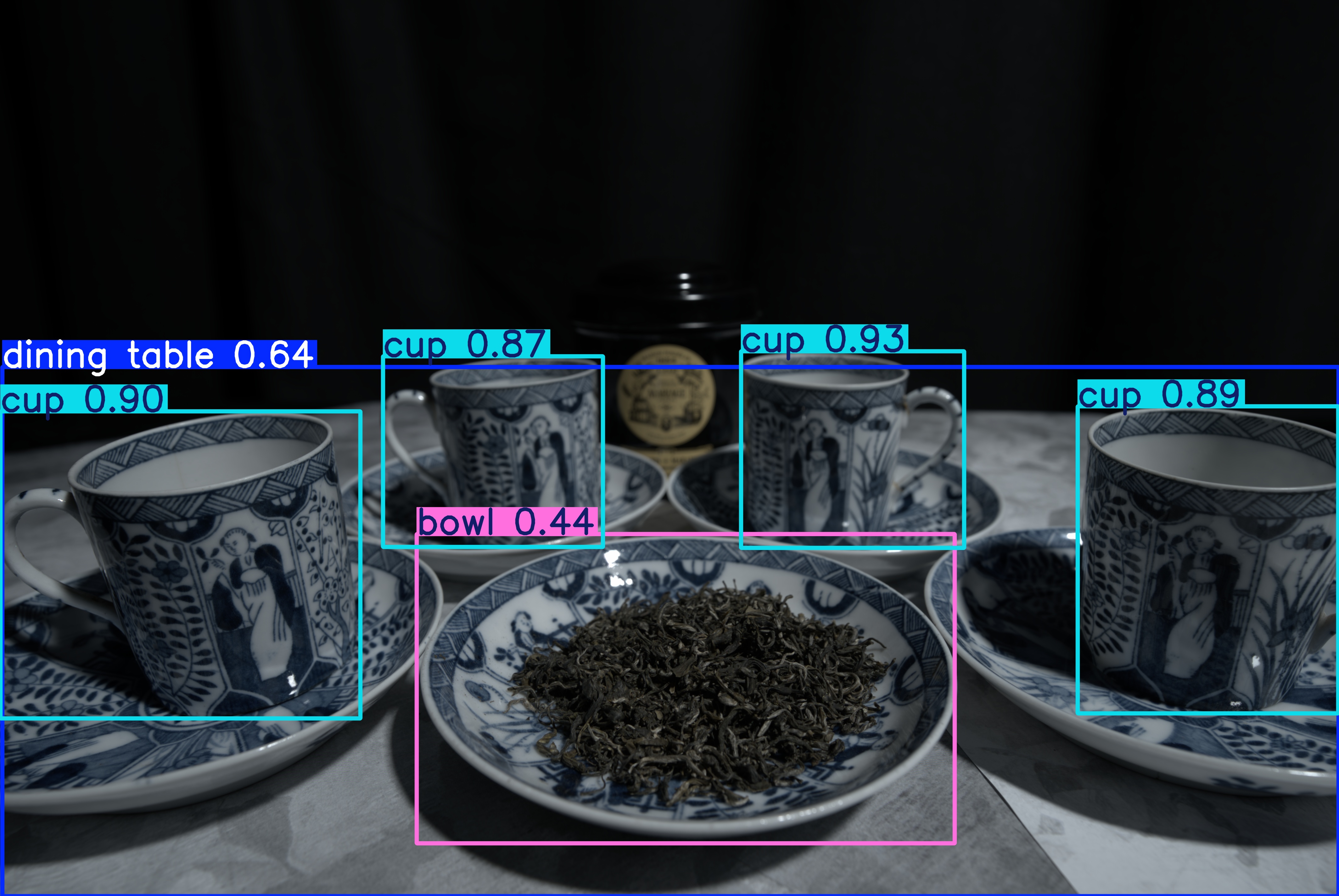
(c) Pre-trained YOLOv11n on clean input.

Figure 7: Qualitative comparison showing the benefits of using our approach to train an object detection model for use in low-light conditions. Our model closely matches the performance of the pre-trained model on the clean scene, without the need for a denoising pre-processing step.

To determine the effectiveness of our synthetic pipeline for downstream tasks separate to video enhancement, we conduct object detection experiments under real low-light conditions. We select the smallest model, ‘nano’, of the ubiquitous YOLOv11 [42] as our test model, due to its excellent performance-to-speed ratio. For each of the four different synthetic pipelines, we train a YOLOv11n model on the popular Microsoft COCO dataset [43]. The synthetic noise is inserted after simulating low-light conditions, using Equation 1. Each model is trained on its respective synthetic low-light data for 100 epochs, and the best hyperparameters are selected from the validation split, which has the same synthetic noise type as the training dataset.

The models are evaluated on the highest ISO Sony frames from the real low-light image dataset [44], which exhibits higher noise levels relative to the other existing real low-light datasets. The performance of each model is tested using pseudo-ground-truth annotations generated by applying the pre-trained YOLOv11n onto the clean ISO-100 videos. In 4 of the 20 scenes, the pre-trained model does not detect any instances of the 80 COCO classes, so those scenes are removed from the test set. We measure this performance using the standard object detection metric of Average Precision (AP), over various Intersection over Union (IoU) thresholds. Specifically, we calculate AP_50-95, in steps of 5, AP₅₀, and AP₇₅.

As shown in Table I (under ‘Object Detection’), training the YOLOv11n model using our training approach results in improved precision across all the thresholds. This demonstrates that our synthetic noise most closely resembles the characteristics of the real low-light test set and enhances the noise handling and feature extraction capabilities of the object detector more effectively. Qualitative results are shown in Fig. 7, along with an example of the limitations of applying a clean model to noisy input. Without training directly on noisy images, the pre-trained YOLOv11n struggles to differentiate cups and bowls, and ignores the presence of a dining table. However, training using our synthetic noise, sampled from the noise vectors predicted by the DEN on the dataset, results in much greater performance.

It is noted that the pre-trained YOLOv11n applied to the clean image is not without fault. It fails to detect the other four bowls in the image with high confidence, and only exhibits particularly high confidence for the cups in the scene. In addition, these three cases exhibit higher performance due to the relatively high light conditions.

4.5 Ablation Study

We characterize the significance of each component in our network through an ablation study. We conduct 3 experiments, each with a different combination of the components, calculating KLD, FID and KID of the noise maps for each experiment. For model v1 in the ablation study, we simply train a U-Net [26] to generate a synthetic noisy image, without employing $f(\cdot)$. This model predictably performs the worst, as the network cannot easily learn to generate appropriate noise characteristics using only a clean input and training data of varying noise characteristics without additional physics-based guidance. For model v2, we consider a network architecture with an encoder and an MLP head. This network was trained to directly estimate the noise vector used to synthesize the noise characteristics from the reference input. This iteration showed some improvements by mostly generating plausible noise, but failed to capture the exact features of the desired noise. Model v3 is the network architecture that we propose for the DEN, comprised of an encoder, with both MLP and decoder heads. This method improves upon model v2 due to the added decoder head and accompanying $\mathcal{L}_{rec}$, forcing the model to learn the specifics of the reference noise.

We highlight the importance of our MLP head, demonstrating a major performance increase when added to the U-Net, with a substantial improvement of 382.916 in FID score between model v1 and model v2, and therefore it is a crucial component for allowing our network to mimic the noise characteristics accurately. Furthermore, we verify that our $\mathcal{L}_{rec}$ improves our network performance by assisting in understanding noise in an image/video. This ablation study confirms the significance of each component in our proposed DEN. The results are shown in Table II.

TABLE II: Ablation Study of the DEN Architecture.

Model	Encoder	Decoder	MLP	KLD$\downarrow$	FID$\downarrow$	KID$\downarrow$
v1	✓	✓	✗	0.425	604.363	1.043
v2	✓	✗	✓	0.379	221.447	0.361
v3	✓	✓	✓	0.347	211.219	0.337

5 Conclusion

We propose a novel general-purpose zero-shot synthetic low-light image and video pipeline which is capable of synthesizing realistic noise from unseen real low-light sources. Unlike other synthetic sRGB deep-learning pipelines, our Degradation Estimation Network does not need information regarding the video capture, enabling seamless application in downstream tasks. Furthermore, our method is applicable to a diverse range of noise characteristics without the need for training targeting individual datasets; making our method easier to generate realistic low-light videos for training deep-learning models. We verify the robustness of our pipeline with our comprehensive study, achieving improvements up to 24% KLD, 21% LPIPS, and 62% AP_50-95.

In our future work, we will focus on video blur, as most existing synthetic pipelines focus on image-only degradations. We would also like to address more complex noise types, such as spatially-correlated noise due to compression, and noise from in-camera processing. Future work could also explore the use of unsupervised algorithms for the network to group similar noise characteristics, to synthesize camera-specific noise patterns without explicit camera information. Furthermore, our model currently focuses on noise synthesis in low-light videos. We would like to expand our method to also map the illumination of the video from normal-light to low-light in a realistic manner, allowing easier low-light synthesis for downstream tasks.

References

- [1] G. A. Sigurdsson, G. Varol, X. Wang, I. Laptev, A. Farhadi, and A. Gupta, “Hollywood in homes: Crowdsourcing data collection for activity understanding,” ArXiv e-prints, 2016. [Online]. Available: http://arxiv.org/abs/1604.01753
- [2] F. Perazzi, J. Pont-Tuset, B. McWilliams, L. Van Gool, M. Gross, and A. Sorkine-Hornung, “A benchmark dataset and evaluation methodology for video object segmentation,” in Computer Vision and Pattern Recognition, 2016.
- [3] N. Xu, L. Yang, Y. Fan, D. Yue, Y. Liang, J. Yang, and T. S. Huang, “Youtube-vos: A large-scale video object segmentation benchmark,” CoRR, vol. abs/1809.03327, 2018. [Online]. Available: http://arxiv.org/abs/1809.03327
- [4] D. Damen, H. Doughty, G. M. Farinella, S. Fidler, A. Furnari, E. Kazakos, D. Moltisanti, J. Munro, T. Perrett, W. Price, and M. Wray, “Scaling egocentric vision: The epic-kitchens dataset,” in European Conference on Computer Vision (ECCV), 2018.
- [5] L. Yang, Y. Fan, and N. Xu, “Video instance segmentation,” in ICCV, 2019.
- [6] L. Huang, X. Zhao, and K. Huang, “Got-10k: A large high-diversity benchmark for generic object tracking in the wild,” IEEE Transactions on Pattern Analysis and Machine Intelligence, vol. 43, no. 5, pp. 1562–1577, 2021.
- [7] N. Anantrasirichai, F. Zhang, and D. Bull, “Artificial intelligence in creative industries: Advances prior to 2025,” 2025. [Online]. Available: https://arxiv.org/abs/2501.02725
- [8] A. Yi and N. Anantrasirichai, “A comprehensive study of object tracking in low-light environments,” arXiv:2312.16250, 2024.
- [9] J. Ye, C. Fu, Z. Cao, S. An, G. Zheng, and B. Li, “Tracker Meets Night: A Transformer Enhancer for UAV Tracking,” IEEE Robotics and Automation Letters, vol. 7, no. 2, pp. 3866–3873, 2022.
- [10] H. Li, J. Wang, J. Yuan, Y. Li, W. Weng, Y. Peng, Y. Zhang, Z. Xiong, and X. Sun, “Event-assisted low-light video object segmentation,” in Proceedings of the IEEE/CVF Conference on Computer Vision and Pattern Recognition (CVPR), June 2024, pp. 3250–3259.
- [11] X. Wang, K. Ma, Q. Liu, Y. Zou, and Y. Fu, “Multi-object tracking in the dark,” in Proceedings of the IEEE/CVF Conference on Computer Vision and Pattern Recognition (CVPR), June 2024, pp. 382–392.
- [12] Y. Liu, A. Mahmood, and M. H. Khan, “Nt-vot211: A large-scale benchmark for night-time visual object tracking,” in Proceedings of the Asian Conference on Computer Vision (ACCV), December 2024, pp. 194–212.
- [13] C. G. Guo, C. Li, J. Guo, C. C. Loy, J. Hou, S. Kwong, and R. Cong, “Zero-reference deep curve estimation for low-light image enhancement,” in Proceedings of the IEEE conference on computer vision and pattern recognition (CVPR), June 2020, pp. 1780–1789.
- [14] R. Wang, X. Xu, C.-W. Fu, J. Lu, B. Yu, and J. Jia, “Seeing dynamic scene in the dark: High-quality video dataset with mechatronic alignment,” in ICCV, 2021.
- [15] H. Fu, W. Zheng, X. Wang, J. Wang, H. Zhang, and H. Ma, “Dancing in the dark: A benchmark towards general low-light video enhancement,” in Proceedings of the IEEE/CVF International Conference on Computer Vision (ICCV), October 2023, pp. 12 877–12 886.
- [16] R. Lin, N. Anantrasirichai, A. Malyugina, and D. Bull, “A spatio-temporal aligned sunet model for low-light video enhancement,” in 2024 IEEE International Conference on Image Processing (ICIP), 2024, pp. 1480–1486.
- [17] J. Lin, N. Anantrasirichai, and D. Bull, “Multi-scale denoising in the feature space for low-light instance segmentation,” in ICASSP 2025 - 2025 IEEE International Conference on Acoustics, Speech and Signal Processing (ICASSP), 2025, pp. 1–5.
- [18] H. Chen and K. Ma, “Enhancing vision: Harmonizing frequency for imaging quality and perception accuracy,” in ICASSP 2025 - 2025 IEEE International Conference on Acoustics, Speech and Signal Processing (ICASSP), April 2025, pp. 1–5.
- [19] A. Foi, M. Trimeche, V. Katkovnik, and K. Egiazarian, “Practical poissonian-gaussian noise modeling and fitting for single-image raw-data,” IEEE Transactions on Image Processing, vol. 17, no. 10, pp. 1737–1754, 2008.
- [20] N. Anantrasirichai, J. Burn, and D. R. Bull, “Robust texture features based on undecimated dual-tree complex wavelets and local magnitude binary patterns,” in 2015 IEEE International Conference on Image Processing (ICIP), 2015, pp. 3957–3961.
- [21] R. Luo, W. Wang, W. Yang, and J. Liu, “Similarity min-max: Zero-shot day-night domain adaptation,” in ICCV, 2023.
- [22] K. Monakhova, S. R. Richter, L. Waller, and V. Koltun, “Dancing under the stars: Video denoising in starlight,” in Proceedings of the IEEE/CVF Conference on Computer Vision and Pattern Recognition (CVPR), June 2022, pp. 16 241–16 251.
- [23] K. Wei, Y. Fu, Y. Zheng, and J. Yang, “Physics-based noise modeling for extreme low-light photography,” IEEE Transactions on Pattern Analysis and Machine Intelligence, vol. 44, no. 11, pp. 8520–8537, 2021.
- [24] Y. Cao, M. Liu, S. Liu, X. Wang, L. Lei, and W. Zuo, “Physics-guided iso-dependent sensor noise modeling for extreme low-light photography,” in Proceedings of the IEEE/CVF Conference on Computer Vision and Pattern Recognition (CVPR), June 2023, pp. 5744–5753.
- [25] F. Zhang, B. Xu, Z. Li, X. Liu, Q. Lu, C. Gao, and N. Sang, “Towards general low-light raw noise synthesis and modeling,” in Proceedings of the IEEE/CVF International Conference on Computer Vision (ICCV), October 2023, pp. 10 820–10 830.
- [26] O. Ronneberger, P. Fischer, and T. Brox, “U-net: Convolutional networks for biomedical image segmentation,” in Medical Image Computing and Computer-Assisted Intervention – MICCAI 2015, N. Navab, J. Hornegger, W. M. Wells, and A. F. Frangi, Eds. Cham: Springer International Publishing, 2015, pp. 234–241.
- [27] S. Kousha, A. Maleky, M. S. Brown, and M. A. Brubaker, “Modeling srgb camera noise with normalizing flows,” in Proceedings of the IEEE/CVF Conference on Computer Vision and Pattern Recognition (CVPR), June 2022, pp. 17 463–17 471.
- [28] Z. Fu, L. Guo, and B. Wen, “srgb real noise synthesizing with neighboring correlation-aware noise model,” in Proceedings of the IEEE/CVF Conference on Computer Vision and Pattern Recognition (CVPR), June 2023, pp. 1683–1691.
- [29] F. Lv, Y. Li, and F. Lu, “Attention guided low-light image enhancement with a large scale low-light simulation dataset,” International Journal of Computer Vision, vol. 129, no. 7, pp. 2175–2193, 2021.
- [30] Z. Cui, G.-J. Qi, L. Gu, S. You, Z. Zhang, and T. Harada, “Multitask aet with orthogonal tangent regularity for dark object detection,” in Proceedings of the IEEE/CVF International Conference on Computer Vision (ICCV), October 2021, pp. 2553–2562.
- [31] S. Zhou, C. Li, and C. C. Loy, “Lednet: Joint low-light enhancement and deblurring in the dark,” in ECCV, 2022.
- [32] A. El Gamal and H. Eltoukhy, “Cmos image sensors,” IEEE Circuits and Devices Magazine, vol. 21, no. 3, pp. 6–20, 2005.
- [33] C. Boncelet, “Chapter 7 - image noise models,” in The Essential Guide to Image Processing, A. Bovik, Ed. Boston: Academic Press, 2009, pp. 143–167. [Online]. Available: https://www.sciencedirect.com/science/article/pii/B978012374457900007X
- [34] F. Rosenblatt, “The perceptron: A probabilistic model for information storage and organization in the brain,” Psychological Review, vol. 65, no. 6, pp. 386–408, 1958.
- [35] M. Heusel, H. Ramsauer, T. Unterthiner, B. Nessler, and S. Hochreiter, “Gans trained by a two time-scale update rule converge to a local nash equilibrium,” in Advances in Neural Information Processing Systems, I. Guyon, U. V. Luxburg, S. Bengio, H. Wallach, R. Fergus, S. Vishwanathan, and R. Garnett, Eds., vol. 30. Curran Associates, Inc., 2017. [Online]. Available: https://proceedings.neurips.cc/paper_files/paper/2017/file/8a1d694707eb0fefe65871369074926d-Paper.pdf
- [36] M. Bińkowski, D. J. Sutherland, M. Arbel, and A. Gretton, “Demystifying MMD GANs,” in International Conference on Learning Representations, 2018. [Online]. Available: https://openreview.net/forum?id=r1lUOzWCW
- [37] A. Abdelhamed, S. Lin, and M. S. Brown, “A high-quality denoising dataset for smartphone cameras,” in IEEE Conference on Computer Vision and Pattern Recognition (CVPR), June 2018.
- [38] R. Lin, N. Anantrasirichai, G. Huang, J. Lin, Q. Sun, A. Malyugina, and D. Bull, “BVI-RLV: A fully registered dataset and benchmarks for low-light video enhancement,” arXiv preprint arXiv:2407.03535, 2024.
- [39] R. Zhang, P. Isola, A. A. Efros, E. Shechtman, and O. Wang, “The unreasonable effectiveness of deep features as a perceptual metric,” in CVPR, 2018.
- [40] J. Wang, K. C. Chan, and C. C. Loy, “Exploring clip for assessing the look and feel of images,” in AAAI, 2023.
- [41] A. Mittal, R. Soundararajan, and A. C. Bovik, “Making a “completely blind” image quality analyzer,” IEEE Signal Processing Letters, vol. 20, no. 3, pp. 209–212, 2013.
- [42] G. Jocher, J. Qiu, and A. Chaurasia, “Ultralytics YOLO,” Jan. 2023. [Online]. Available: https://github.com/ultralytics/ultralytics
- [43] T.-Y. Lin, M. Maire, S. Belongie, J. Hays, P. Perona, D. Ramanan, P. Dollár, and C. L. Zitnick, “Microsoft coco: Common objects in context,” in European Conference on Computer Vision, 2014, pp. 740–755.
- [44] N. Anantrasirichai, R. Lin, A. Malyugina, and D. Bull, “Bvi-lowlight: Fully registered benchmark dataset for low-light video enhancement,” arXiv preprint arXiv:2402.01970, 2024.