$D^{0}-\bar{D}^{0}$ mixing in the Dyson-Schwinger approach

Abstract

In view of difficulty to reproduce observables in the $D^{0}-\bar{D}^{0}$ mixing via the operator product expansion, we discuss the Dyson-Schwinger approach to this process. Formulated by the parameterization of quark propagators, SU(3) breaking relevant to charm mixing is evaluated in such a way that properly takes account of dynamical chiral symmetry breaking. The $\bar{D}^{0}\to D^{0}$ transition is discussed in the vacuum-insertion approximation with locality of the light valence-quark field, represented by the decay constant of $D^{0}$ meson as well as relevant momentum integrals. It is found that dimensionless mass-difference observable in this approach leads to $|x|=(1.3-2.9)\times 10^{-3}$, the order of magnitude comparable to the HFLAV data, and thereby offering a certain improvement as a theoretical framework.

I Introduction

Owing to the notable development of heavy quark physics in 90’s, strong interaction of $b$ quark system can be systematically handled, which enables us to analyze a variety of observables to date. Armed with those formulations, precise determinations of the Cabibbo-Kobayashi-Maskawa (CKM) matrix elements Cabibbo:1963yz , as well as search for physics beyond the standard model, have been implemented in recent flavor-factory experiments. In contrast to the mature status in $B$-meson system, however, there still exist difficulties in regards to the charm sector. In particular, dominance of long-distance effects for the $D^{0}-\bar{D}^{0}$ mixing has been remarked Donoghue:1985hh , and therefore requiring dedicated analysis incorporating nonperturbative dynamics.

The conventional theoretical methods for the $D^{0}-\bar{D}^{0}$ mixing are classified as two types: The exclusive and inclusive approaches. The former offers parametrization of decay amplitudes, with specific methods given by topological diagram approach Cheng:2010rv ; Cheng:2024hdo , factorization-assisted topological approach Jiang:2017zwr or flavor symmetry approach Gronau:2012kq and yields the data-driven formalism to predicts the observables in the $D^{0}-\bar{D}^{0}$ mixing. This methodology takes finite sum over hadronic intermediate states of $\bar{D^{0}}\to\textrm{hadrons}\to D^{0}$, reproducing approximately a half of the experimental data relevant to width difference Cheng:2010rv ; Jiang:2017zwr ; Cheng:2024hdo .

As for the inclusive approach Golowich:2005pt ; Bobrowski:2010xg (a recent work is found in Ref. Melic:2024oqj ), the primary formulation is based on the operator product expansion (OPE) Wilson:1969zs . In a sharp contrast to the mentioned status in the exclusive approach, the inclusive one gives predictions that are much smaller than the experimental data: If we take a dimensionless mass-difference observable as an example, the comparison between the OPE value at the next-to-leading order (NLO) in Ref. Golowich:2005pt and the experimental result from the heavy flavor averaging group (HFLAV) HeavyFlavorAveragingGroupHFLAV:2024ctg reads,

$$x_{\rm Th.}=6\times 10^{-7},\qquad x_{\rm Exp.}=(4.07\pm 0.44)\times 10^{-3},$$ (1)

where the definition of $x$ is properly introduced later in Sec. II.1. As shown in Eq. (1), there exists a gap between the two results in four orders of magnitude.

The difficulty in reproducing the data for the inclusive approach is attributed to the extreme suppression that originates from the Glashow-Iliopoulos-Maiani (GIM) mechanism Glashow:1970gm . As a consequence of this, in the limit where the product of the CKM matrix elements $(V_{cb}V_{ub}^{*})$ vanishes, the observables in the $D^{0}-\bar{D}^{0}$ mixing are proportional to SU(3) breaking as was remarked in Ref. Kingsley:1975fe . In order to capture the relevant size of the observables, proper evaluation of hadronic (or nonperturbative) SU(3) breaking plays a crucial role. See Refs. Bigi:2000wn ; Bobrowski:2010xg ; Falk:2001hx ; Falk:2004wg for further discussions.

For the $c\to u\gamma$ decay, the difficulty similar to the $D^{0}-\bar{D}^{0}$ mixing is also found: In Ref. Greub:1996wn , branching ratio of inclusive radiative decay, $\Delta\textrm{Br}[D^{0}\xrightarrow{\Delta S=0}X\gamma]_{c\to u\gamma}$, is obtained as $2.5\times 10^{-8}$, much smaller than the particle data group (PDG) value of one exclusive channel, $\textrm{Br}[D^{0}\to\rho^{0}\gamma]=(1.82\pm 0.32)\times 10^{-5}$ ParticleDataGroup:2024cfk . For this, robust enhancement of the result is confirmed Greub:1996wn , if one replaces the current-quark masses for $s$ and $d$ quarks by ones of the constituent-quark masses. Even though the process is different, a similar enhancement in a larger magnitude is expected for charm mixing. Furthermore, for the $D^{0}-\bar{D}^{0}$ mixing in the OPE-based approaches, the condensate contributions Bigi:2000wn , as well as nonlocal chiral condensates Melic:2024oqj , are discussed as power-suppressed terms that can avoid severe GIM suppression, and thereby leading to large corrections. Those previous works generically imply the importance of chiral symmetry breaking in charm mixing.

In this work, we evaluate an observable in the $D^{0}-\bar{D}^{0}$ mixing based on the Dyson-Schwinger equation (DSE) approach Roberts:1994dr . Formulated by the propagators for intermediate $d$ and $s$ quarks, the dimensionless mass-difference parameter is analyzed, with SU(3) breaking properly incorporated. To this end, the parametrization Burden:1991gd ; Burden:1995ve ; Kalinovsky:1996ii ; Ivanov:1997yg ; Ivanov:1998ms accommodating confinement and dynamical chiral symmetry breaking (DCSB) as well as asymptotic freedom is adopted. This framework enables us to estimate the size of observables with nonperturbative SU(3) breaking via the relevant momentum integrals of the quark propagators.

This paper is organized as follows: In Sec. II.1, theoretical formulae for the $D^{0}-\bar{D^{0}}$ mixing, as well as definitions of mixing parameters, are introduced. In Sec. II.2, the OPE approach to the $D^{0}-\bar{D^{0}}$ mixing is briefly recapitulated. In Sec. II.3, SU(3) breaking that originates from the GIM mechanism is discussed with some replacements of quark masses. In Sec. III, the mixing parameter is estimated in the DSE approach, giving numerical results in this work. The concluding remarks are addressed in Sec. IV.

II $D^{0}-\bar{D}^{0}$ mixing

II.1 Mixing parameters

Here formulae for charm mixing are given in the CPT-conserving limit HeavyFlavorAveragingGroupHFLAV:2024ctg . Taking the phase convention of CP transform as $\textrm{CP}\ket{D^{0}}=-\ket{\bar{D}^{0}}$, we introduce mass eigenstates,

$$\ket{D_{1,2}} = p\ket{D^{0}}\mp q\ket{\bar{D}^{0}},$$ (2)

where $|p|^{2}+|q|^{2}=1$. In the CP-conserving case of $p=q$, $D_{1}~(D_{2})$ is reduced to a CP-even (CP-odd) state. The matrix element for the $\bar{D}^{0}\to D^{0}$ transition is divided into the dispersive and absorptive parts,

$$M_{12}-\frac{i}{2}\Gamma_{12} = \frac{\braket{D^{0}|\mathcal{H}_{\rm eff}|\bar{D}^{0}}}{2M_{D^{0}}},\qquad\mathcal{H}_{\rm eff}=\mathcal{H}_{\rm disp}-\frac{i}{2}\mathcal{H}_{\rm abs},$$ (3)

or equivalently,

$$M_{12} = \frac{\braket{D^{0}|\mathcal{H}_{\rm disp}|\bar{D}^{0}}}{2M_{D^{0}}},\qquad\Gamma_{12}=\frac{\braket{D^{0}|\mathcal{H}_{\rm abs}|\bar{D}^{0}}}{2M_{D^{0}}}.$$ (4)

In our convention, $D^{0}$ and $\bar{D}^{0}$ states are relativistically normalized,

$$\braket{D^{0}(\mathbf{p})|D^{0}(\mathbf{p}^{\prime})}=\braket{\bar{D}^{0}(\mathbf{p})|\bar{D}^{0}(\mathbf{p}^{\prime})}=2E_{\mathbf{p}}(2\pi)^{3}\delta^{(3)}(\mathbf{p}-\mathbf{p}^{\prime}).$$ (5)

The observables are defined by,

$$x=\displaystyle\frac{\Delta m}{\Gamma},\qquad y=\displaystyle\frac{\Delta\Gamma}{2\Gamma},$$ (6)

$$\Delta m=m_{1}-m_{2},\qquad\Delta\Gamma=\Gamma_{1}-\Gamma_{2},\qquad\Gamma=\displaystyle\frac{\Gamma_{1}+\Gamma_{2}}{2}.$$ (7)

In what follows, we take the CP-conserving limit, leading to,

$$M_{12}=\textrm{Re}\displaystyle\frac{\braket{D^{0}|\mathcal{H}_{\rm eff}|\bar{D}^{0}}}{2M_{D^{0}}},\qquad\Gamma_{12}=-2\textrm{Im}\frac{\braket{D^{0}|\mathcal{H}_{\rm eff}|\bar{D}^{0}}}{2M_{D^{0}}}.$$ (8)

The effective Hamiltonian for the $\Delta C=1$ transition is defined by,

$$\mathcal{H}_{\rm eff} = \frac{(-i)^{2}}{2!}i\int\textrm{T}[\mathcal{H}_{\Delta C=1}(x)\mathcal{H}_{\Delta C=1}(0)]d^{4}x.$$ (9)

In the case where CKM-suppressed contributions of $b$ quark are neglected, the Hamiltonian reads,

$$\mathcal{H}_{\Delta C=1} = \displaystyle\sum_{i=d}^{s}\displaystyle\sum_{j=d}^{s}\mathcal{H}_{ij},$$ (10)

$$\mathcal{H}_{ij} = \frac{4G_{F}}{\sqrt{2}}V_{ci}V_{uj}^{*}(C_{1}O_{1}+C_{2}O_{2}),$$ (11)

$$O_{1} = (\bar{c}^{\alpha}\gamma^{\mu}P_{L}q^{\beta}_{i})(\bar{q}^{\beta}_{j}\gamma_{\mu}P_{L}u^{\alpha}),$$ (12)

$$O_{2} = (\bar{c}^{\alpha}\gamma^{\mu}P_{L}q^{\alpha}_{i})(\bar{q}^{\beta}_{j}\gamma_{\mu}P_{L}u^{\beta}).$$ (13)

The sum over color indices denoted as $\alpha$ and $\beta$ are understood in Eqs. (12, 13). In what follows, the dispersive part, which is of our current interest, is analyzed.

II.2 OPE approach

We recapitulate the conventional inclusive approach Hagelin:1981zk ; Cheng:1982hq ; Buras:1984pq ; Datta:1984jx ; Golowich:2005pt ; Bobrowski:2010xg at the leading order (LO). One can implement the replacement,

$$\mathcal{H}_{\Delta C=1}(x)\mathcal{H}_{\Delta C=1}(0)\to\displaystyle\sum_{i,j}^{d,s}\mathcal{H}_{ij}(x)\mathcal{H}_{ji}(0).$$ (14)

Furthermore, with $\lambda_{i}=V_{ci}V_{ui}^{*}$, the unitarity of the CKM matrix leads to,

$$\lambda_{d}+\lambda_{s}+\lambda_{b}=0.$$ (15)

In the limit of $\lambda_{b}\simeq 0$, one can eliminate $\lambda_{d}$ and write the result only in terms of $\lambda_{s}$. This procedure renders Eq. (9) recast into the form (see, e.g., Ref. Golowich:2005pt ),

$$\mathcal{H}_{\rm disp} \simeq -\frac{G_{F}^{2}m_{c}^{2}}{8\pi^{2}}\lambda_{s}^{2}[C_{2}^{2}Q_{1}+2(C_{2}^{2}-2C_{1}C_{2}-N_{c}C_{1}^{2})Q_{2}]\left(\frac{m_{s}^{2}-m_{d}^{2}}{m_{c}^{2}}\right)^{2},$$ (16)

$$Q_{1} = [\bar{c}^{\alpha}\gamma^{\mu}(1-\gamma^{5})u^{\alpha}][\bar{c}^{\beta}\gamma^{\mu}(1-\gamma^{5})u^{\beta}],$$ (17)

$$Q_{2} = [\bar{c}^{\alpha}(1-\gamma^{5})u^{\alpha}][\bar{c}^{\beta}(1-\gamma^{5})u^{\beta}],$$ (18)

where $Q_{i}~(i=1,2)$ is the $\Delta C=2$ operator. The matrix elements for Eqs. (17, 18) are defined with bag parameters,

$$\braket{D^{0}|Q_{1}|\bar{D}^{0}} = \frac{8}{3}M_{D^{0}}^{2}f_{D^{0}}^{2}B_{1},$$ (19)

$$\braket{D^{0}|Q_{2}|\bar{D}^{0}} = -\frac{5}{3}\left(\frac{M_{D^{0}}}{m_{c}+m_{u}}\right)^{2}M_{D^{0}}^{2}f_{D^{0}}^{2}B_{2},$$ (20)

leading to ($N_{c}=3$),

$$M_{12} \simeq -\frac{G_{F}^{2}f_{D^{0}}^{2}M_{D^{0}}m_{c}^{2}}{6\pi^{2}}\lambda_{s}^{2}\left[C_{2}^{2}B_{1}-\frac{5}{4}(C_{2}^{2}-2C_{1}C_{2}-N_{c}C_{1}^{2})\left(\frac{M_{D^{0}}}{m_{c}+m_{u}}\right)^{2}B_{2}\right]\left(\frac{m_{s}^{2}-m_{d}^{2}}{m_{c}^{2}}\right)^{2}.\qquad$$ (21)

It is evident that $M_{12}$ vanishes in the SU(3) limit, $m_{s}=m_{d}$, as a consequence of the GIM mechanism with $\lambda_{b}=0$.

II.3 GIM suppression factor

One can estimate the size of the last factor in Eq. (21): If one fixes masses for $s$, $d$ and $c$ to the $\overline{\rm MS}$ masses at the scale of charm quark mass, where renormalization group evolution (RGE) for $m_{s}$ and $m_{d}$ are evaluated by RunDec Chetyrkin:2000yt with input parameters of $m_{c}(m_{c})$, $m_{d}(2~\textrm{GeV})$ and $m_{s}(2~\textrm{GeV})$ in Ref. ParticleDataGroup:2024cfk , we obtain,

$$\left(\frac{m_{s}^{2}-m_{d}^{2}}{m_{c}^{2}}\right)^{2}=5.2\times 10^{-5},$$ (22)

giving the extreme suppression in Eq. (21).

Here we consider the replacement of the current-quark masses by the constituent-quark masses similarly to Ref. Greub:1996wn for $c\to u\gamma$ decays. Specifically, the constituent-quark mass in the relativistic constituent quark model (RCQM) Schlumpf:1992vq and the Euclidean constituent-quark mass, obtained as a solution of $M^{2}(p^{2}_{E})=p^{2}_{E}$ with $M(p^{2}_{E})$ determined in the DSE approach Ivanov:1998ms , are adopted for illustrating the size of the factor. If we take $m_{s}^{\rm con}=0.49~\textrm{GeV}~\textrm{and}~m_{d}^{\rm con}=0.36~\textrm{GeV}$ Ivanov:1998ms as an example, the factor corresponding to Eq. (22) is,

$$\left[\frac{(m_{s}^{\rm con})^{2}-(m_{d}^{\rm con})^{2}}{m_{c}^{2}}\right]^{2}=4.6\times 10^{-3},$$ (23)

which is two orders of magnitude larger than Eq. (22). The resulting observable is also enhanced by the mentioned factor.

In order to obtain the numerical result, we adopt $M_{D^{0}}=1.86484~\textrm{GeV}$ in PDG ParticleDataGroup:2024cfk and $f_{D^{0}}=0.2120~\textrm{GeV}$ in lattice QCD Carrasco:2014poa (see also FlavourLatticeAveragingGroupFLAG:2024oxs ). As to the CKM matrix elements in the CP-conserving limit, we adopt the absolute values in PDG, $|V_{cs}|=0.975$ and $|V_{us}|=0.22431$ ParticleDataGroup:2024cfk for $\lambda_{s}^{2}$ in Eq. (21). For the bag parameters, they are computed via lattice QCD in Refs. Gupta:1996yt ; Carrasco:2014uya ; Carrasco:2015pra ; Bazavov:2017weg , with central values of Ref. Carrasco:2015pra in Eqs. (55, 56, 57) adopted for our analysis. The corrections from RGE to the bag parameters and the Wilson coefficients are given in App. A. The $u$ quark mass in Eq. (21) is fixed to the $\overline{\rm MS}$ mass at the scale of $m_{c}$ via the RunDec Chetyrkin:2000yt .

In Tab. 1, values of $|x|$ with different masses for $s$ and $d$ quarks are compared. As can be seen in Tab. 1, the cases with constituent-quark masses give larger $|x|$ than that with the $\overline{\rm MS}$ masses. The resulting enhancement is highly sensitive to the values of $m_{s}^{\rm con}$ and $m_{d}^{\rm con}$.

Table 1: The dimensionless mass-difference observable $(|x|)$ with different values of quark-mass parameters: (a) $\overline{\rm MS}$ mass. (b) (c) and (f) RCQM with the harmonic oscillator wavefunction. (d) Constituent-quark mass adopted in $c\to u\gamma$ study. (e) and (g) the Euclidean constituent-quark mass in the DSE approach. For the constituent-quark masses, the isospin limit, $m_{u}^{\rm con}=m_{d}^{\rm con}$, is adopted.

	$|x|$	$m_{s}^{(\textrm{con})}/\textrm{GeV}$	$m_{d}^{(\textrm{con})}/\textrm{GeV}$	Method/Model	Reference
(a)	$2.5\times 10^{-6}$	$0.108$	0.0055	$\overline{\rm MS}$ mass	ParticleDataGroup:2024cfk ; Chetyrkin:2000yt
(b)	$1.1\times 10^{-4}$	$0.38$	0.26	RCQM	Schlumpf:1992vq
(c)	$1.5\times 10^{-4}$	$0.40$	0.267	RCQM	Schlumpf:1992vq
(d)	$2.3\times 10^{-4}$	$0.45$	0.30	Constituent-quark mass	Greub:1996wn
(e)	$2.3\times 10^{-4}$	$0.49$	0.36	DSE	Ivanov:1998ms
(f)	$6.9\times 10^{-4}$	$0.55$	0.33	RCQM	Schlumpf:1992vq
(g)	$5.8\times 10^{-4}$	$0.70$	0.56	DSE	Ivanov:1998ms

It should be noted, however, that momentum dependence of the quark propagators is not fully incorporated in the simple replacement for the quark masses in Eq. (23) and also in the numerical results of Tab. 1 (b)-(g). In the next section, the integral over the relevant momenta is carried out using the DSE approach.

III DSE approach

III.1 Quark propagator

The quark propagator in the Minkowski notation is denoted as,

$$S_{i}(x,y)=\int\frac{d^{4}p}{(2\pi)^{4}}i[\not{p}\sigma_{V}^{i}(-p^{2})+\sigma_{S}^{i}(-p^{2})]e^{-ip\cdot(x-y)}.\quad(i=d,s)$$ (24)

In Eq. (24), $\sigma_{V}^{i}(-p^{2})$ and $\sigma_{S}^{i}(-p^{2})$ represent the vector and the scalar parts, respectively, with the sign of the argument taken as negative for the later convenience of the Euclidean notation. In Refs. Burden:1991gd ; Burden:1995ve ; Kalinovsky:1996ii ; Ivanov:1997yg ; Ivanov:1998ms , the parameterization of the $\sigma_{V,\>S}$ has been discussed. One can incorporate DCSB, which is not explicitly seen for the OPE at the leading power approximation, in this method. Color confinement is also accommodated in the sense that the parameterization does not possess the Lehmann representation Burden:1991gd . The explicit forms for $\sigma_{V,\>S}$ are given by Burden:1991gd ; Burden:1995ve ; Kalinovsky:1996ii ; Ivanov:1997yg ; Ivanov:1998ms ,

$$\sigma_{V}^{i}(p_{E}^{2}) = \frac{\bar{\sigma}_{V}^{i}(x)}{2D},\qquad\sigma_{S}^{i}(p_{E}^{2})=\frac{\bar{\sigma}_{S}^{i}(x)}{\sqrt{2D}},$$ (25)

$$\bar{\sigma}_{V}^{i}(x) = \frac{2(x+\bar{m}_{i}^{2})-1+e^{-2(x+\bar{m}_{i}^{2})}}{2(x+\bar{m}_{i}^{2})^{2}},$$ (26)

$$\bar{\sigma}_{S}^{i}(x) = 2\bar{m}_{i}\mathcal{F}(2(x+\bar{m}_{i}^{2}))+\mathcal{F}(b_{1}^{i}x)\mathcal{F}(b_{3}^{i}x)[b_{0}^{i}+b_{2}^{i}\mathcal{F}(\epsilon x)],$$ (27)

where $p_{E}^{2}=-p^{2}$, $x=p_{E}^{2}/(2D),\bar{m}_{i}=\tilde{m}_{i}/\sqrt{2D}$ and $\mathcal{F}(z)=(1-e^{-z})/z$ while $b_{n}^{i}~(n=0,1,2,3),D$ and $\epsilon$ are parameters determined in the previous work Ivanov:1997yg .

In order to illustrate typical momentum dependence of the quark propagators, $\sigma_{S}/\sigma_{V}$, corresponding to the quark mass function, is plotted in Fig. 1, clearly showing DCSB. The parameters in Eqs. (25, 26, 27) are fixed by Ivanov:1997yg $D=0.160~\textrm{GeV}$, $\epsilon=10^{-4}$ and,

$$\tilde{m}_{u}=0.00897~\textrm{GeV},~b_{0}^{u}=0.131,~b_{1}^{u}=2.90,b_{2}^{u}=0.603,~b_{3}^{u}=0.185,$$ (28)

$$\tilde{m}_{s}=0.224~\textrm{GeV},~b_{0}^{s}=0.105,~b_{1}^{s}=2.90,b_{2}^{s}=0.740,~b_{3}^{s}=0.185.$$ (29)

We take the isospin limit for Eq. (28), i.e., the equality of the parameters for $u$ and $d$ quarks.

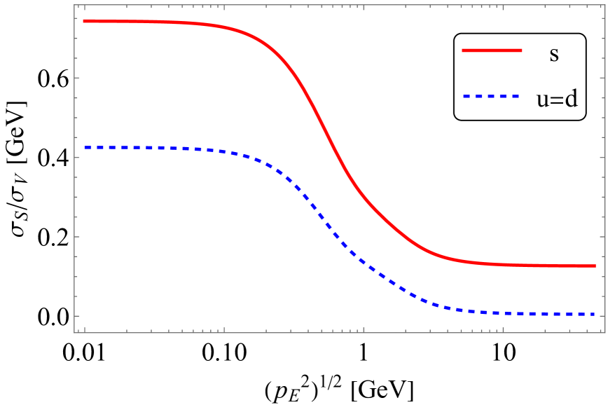
Figure 1: Momentum dependence of $\sigma_{S}/\sigma_{V}$ in the DSE approach based on the previous work Ivanov:1997yg .

III.2 Dispersive part of $\bar{D}^{0}\to D^{0}$ transition

By implementing the Fierz transform, the $\Delta C=1$ operator in Eq. (12) is rewritten by,

$$O_{1} = (\bar{c}^{\alpha}\gamma^{\mu}P_{L}u^{\alpha})(\bar{q}^{\beta}_{j}\gamma_{\mu}P_{L}q^{\beta}_{i}).$$ (30)

Hereafter, the operator basis in Eqs. (30) and (13) are used for analyzing the $D^{0}-\bar{D}^{0}$ mixing. In this case, the color flow and the flavor flow are identical in a given diagram.

Contributions to the dispersive Hamiltonian are divided into four parts from the $\Delta C=1$ operators (sum over $i,j=d,s$ is not taken),

$$M_{12}^{ij} = \frac{2iG_{F}^{2}}{M_{D}}\lambda_{i}\lambda_{j}\int d^{4}x\>\textrm{tr}[X_{\mu\nu}^{ij}(x)]$$ (31)

$$\times \{N_{c}C_{1}^{2}\bra{D^{0}}T[\bar{c}^{\alpha}(x)\gamma^{\mu}P_{L}u^{\alpha}(x)][\bar{c}^{\beta}(0)\gamma^{\nu}P_{L}u^{\beta}(0)]\ket{\bar{D}^{0}}$$

$$+ C_{2}^{2}\bra{D^{0}}T[\bar{c}^{\alpha}(x)\gamma^{\mu}P_{L}u^{\beta}(x)][\bar{c}^{\beta}(0)\gamma^{\nu}P_{L}u^{\alpha}(0)]\ket{\bar{D}^{0}}$$

$$+ C_{1}C_{2}\bra{D^{0}}T[\bar{c}^{\alpha}(x)\gamma^{\mu}P_{L}u^{\alpha}(x)][\bar{c}^{\beta}(0)\gamma^{\nu}P_{L}u^{\beta}(0)]\ket{\bar{D}^{0}}$$

$$+ C_{2}C_{1}\bra{D^{0}}T[\bar{c}^{\alpha}(x)\gamma^{\mu}P_{L}u^{\alpha}(x)][\bar{c}^{\beta}(0)\gamma^{\nu}P_{L}u^{\beta}(0)]\ket{\bar{D}^{0}}\}.$$

As shown above, the terms proportional to $C_{1}C_{2}$ and $C_{2}C_{1}$ yield identical contributions. In Eq. (31), the intermediate flavor dependence, represented by the indices of $i$ and $j$, is included only in $\lambda_{i}\lambda_{j}$ and $X_{\mu\nu}^{ij}$ defined by,

$$X_{\mu\nu}^{ij}(x)=S_{i}(0,x)\gamma_{\mu}P_{L}S_{j}(x,0)\gamma_{\nu}P_{L}.$$ (32)

In Eq. (31), the trace denoted as $\textrm{tr}[X_{\mu\nu}^{ij}(x)]$ runs over only the Dirac indices, not for color or flavor indices. It should be noted that $\sigma_{S}$ in Eq. (24) does not contribute to $\textrm{tr}[X_{\mu\nu}^{ij}(x)]$ due to its chirality structure, similarly to the conventional OPE analysis at LO.

In order to estimate Eq. (31), one inserts vacua in between the two currents for the matrix element, corresponding to the vacuum-insertion approximation (VIA). At this stage, care must be taken for multiple ways of contracting fermion fields in the matrix element to valence quarks in the $D$-meson states, leading to

$$\bra{D^{0}}T[\bar{c}^{\alpha}(x)\gamma^{\mu}P_{L}u^{\alpha}(x)][\bar{c}^{\beta}(0)\gamma^{\nu}P_{L}u^{\beta}(0)]\ket{\bar{D}^{0}}$$ (33)

$$\simeq \bra{D^{0}}\bar{c}^{\alpha}(x)\gamma^{\mu}P_{L}u^{\alpha}(x)\ket{0}\bra{0}\bar{c}^{\beta}(0)\gamma^{\nu}P_{L}u^{\beta}(0)\ket{\bar{D}^{0}}$$

$$+ \bra{D^{0}}\bar{c}^{\beta}(0)\gamma^{\nu}P_{L}u^{\beta}(0)\ket{0}\bra{0}\bar{c}^{\alpha}(x)\gamma^{\mu}P_{L}u^{\alpha}(x)\ket{\bar{D}^{0}}$$

$$- \bra{D^{0}}\bar{c}_{a}^{\alpha}(x)u_{d}^{\beta}(0)\ket{0}\bra{0}\bar{c}_{c}^{\beta}(0)u_{b}^{\alpha}(x)\ket{\bar{D}^{0}}(\gamma^{\mu}P_{L})_{ab}(\gamma^{\nu}P_{L})_{cd}$$

$$- \bra{D^{0}}\bar{c}_{c}^{\beta}(0)u^{\alpha}_{b}(x)\ket{0}\bra{0}\bar{c}_{a}^{\alpha}(x)u^{\beta}_{d}(0)\ket{\bar{D}^{0}}(\gamma^{\mu}P_{L})_{ab}(\gamma^{\nu}P_{L})_{cd},$$

where $a,b,c$ and $d$ represent the Dirac indices. For the third and fourth terms in Eq. (33), one can rearrange the color indices,

$$[\bar{c}^{\alpha}u^{\beta}][\bar{c}^{\beta}u^{\alpha}] = \frac{1}{N_{c}}[\bar{c}^{\alpha}u^{\alpha}][\bar{c}^{\beta}u^{\beta}]+2[\bar{c}^{\alpha}T^{a}_{\alpha\beta}u^{\beta}][\bar{c}^{\gamma}T^{a}_{\gamma\delta}u^{\delta}],$$ (34)

which follows from $T^{a}_{\alpha\beta}T^{a}_{\gamma\delta}=(\delta_{\alpha\delta}\delta_{\gamma\beta}-\delta_{\alpha\beta}\delta_{\gamma\delta}/N_{c})/2$. Since the Bethe-Salpeter amplitude is diagonal in color indices, $\bra{\bar{D^{0}}}u^{\alpha}\bar{c}^{\beta}\ket{0}\propto\delta^{\alpha\beta}$ (see, e.g., Ref. Kugo:1993rd ), the matrix element of the second term in Eq. (34) vanishes due to $\textrm{tr}(T^{a})=0$. Furthermore, for the third and fourth terms in Eq. (33), one can implement the Fierz transform,

$$(\gamma^{\mu}P_{L})_{ab}(\gamma^{\nu}P_{L})_{cd}=\frac{1}{2}(\gamma^{\mu}\gamma^{\rho}\gamma^{\nu}P_{L})_{ad}(\gamma_{\rho}P_{L})_{cb}.$$ (35)

By noting that parity must be preserved so that the matrix element of the form, $\bra{D^{0}}\bar{c}\gamma^{\mu}u\ket{0}$, vanishes, we rewrite Eq. (33),

$$\bra{D^{0}}T[\bar{c}^{\alpha}(x)\gamma^{\mu}P_{L}u^{\alpha}(x)][\bar{c}^{\beta}(0)\gamma^{\nu}P_{L}u^{\beta}(0)]\ket{\bar{D}^{0}}$$ (36)

$$\simeq \frac{1}{4}\bra{D^{0}}\bar{c}^{\alpha}(x)\gamma^{\mu}\gamma^{5}u^{\alpha}(x)\ket{0}\bra{0}\bar{c}^{\beta}(0)\gamma^{\nu}\gamma^{5}u^{\beta}(0)\ket{\bar{D}^{0}}$$

$$+ \frac{1}{4}\bra{D^{0}}\bar{c}^{\beta}(0)\gamma^{\nu}\gamma^{5}u^{\beta}(0)\ket{0}\bra{0}\bar{c}^{\alpha}(x)\gamma^{\mu}\gamma^{5}u^{\alpha}(x)\ket{\bar{D}^{0}}$$

$$- \frac{1}{2N_{c}}\bra{D^{0}}\bar{c}^{\alpha}(x)\gamma^{\mu}\gamma^{\rho}\gamma^{\nu}P_{L}u^{\alpha}(0)\ket{0}\bra{0}\bar{c}^{\beta}(0)\gamma_{\rho}P_{L}u^{\beta}(x)\ket{\bar{D}^{0}}$$

$$- \frac{1}{2N_{c}}\bra{D^{0}}\bar{c}^{\alpha}(0)\gamma_{\rho}P_{L}u^{\alpha}(x)\ket{0}\bra{0}\bar{c}^{\beta}(x)\gamma^{\mu}\gamma^{\rho}\gamma^{\nu}P_{L}u^{\beta}(0)\ket{\bar{D}^{0}}.$$

Formulas similar to Eq. (36) are found for the terms proportional to $C^{2}_{2},C_{1}C_{2}$ and $C_{2}C_{1}$ in Eq. (31) due to the analogous procedure.

By using the decomposition in Eq. (36), one finds that the Hamiltonian in Eq. (9) includes diagrams in Fig. 2. As shown in the figure, there are eight types of diagrams, corresponding to terms proportional to $C_{1}^{2},C_{2}^{2},C_{1}C_{2}$ and $C_{2}C_{1}$, each of which has two types of different contractions, explicitly displayed in Fig. 2. $N_{c}$ dependence of each diagram can be read off by counting the number of color traces. In addition to those diagrams, there are further eight diagrams, where the roles of the two $\Delta C=1$ vertices are simply interchanged for each of A-H, which we denote A^′-H^′.

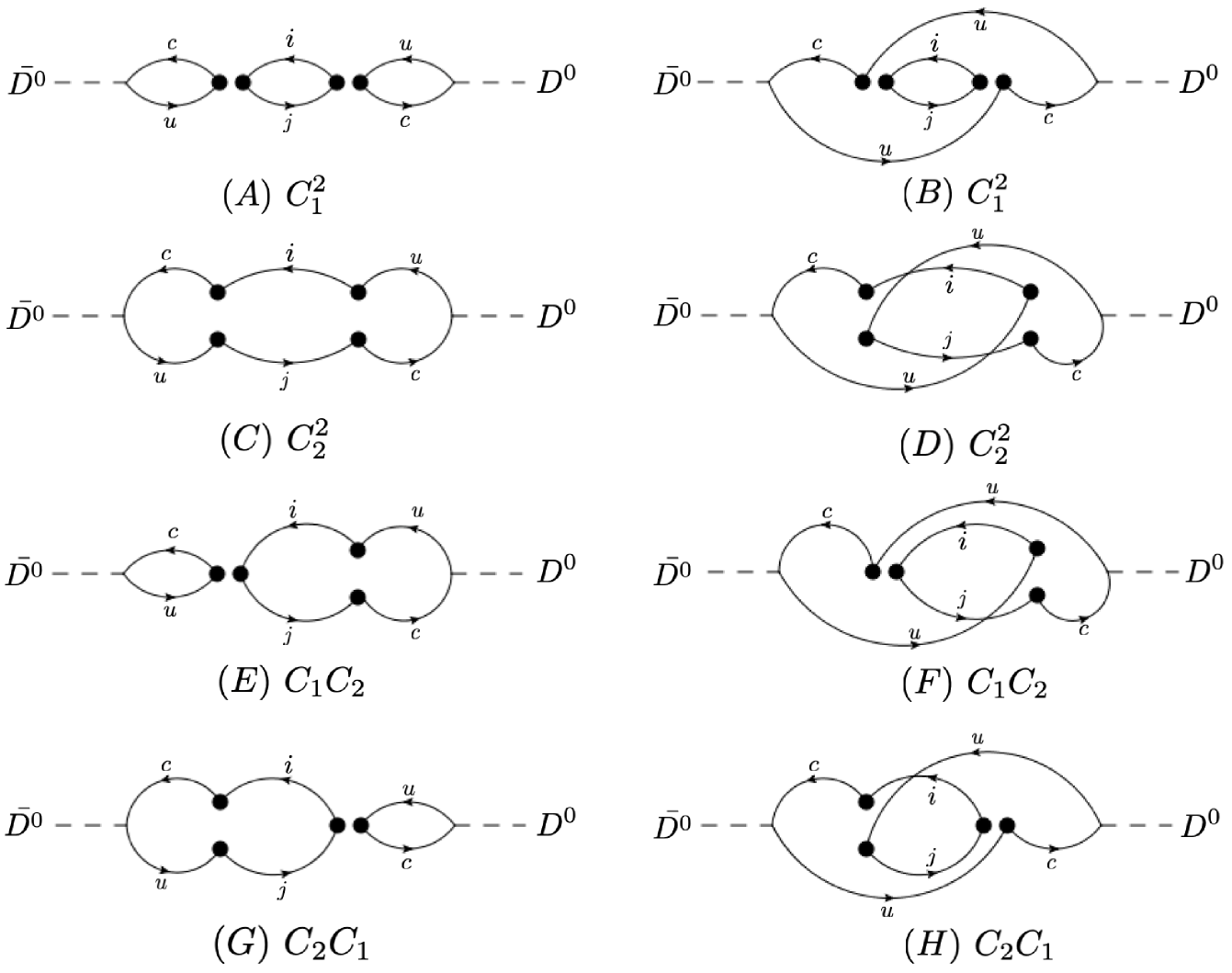
Figure 2: Diagrams for $\bar{D}^{0}\to D^{0}$ transition in the DSE approach with $i,j=d,s$. The black dots denote the Dirac matrix of the form, $\gamma^{\mu}P_{L}$. The fermion lines represent dressed quark propagators with the arrows denoting flavor and color flows. The similar diagrams where the roles of the left and right vertices are interchanged are not displayed.

By evaluating the left-side of the diagrams plus corresponding primed ones in Fig. 2, partial contributions to $M_{12}$ are,

$$M_{12}^{ij}|_{A+A^{\prime}} = N_{c}C_{1}^{2}N_{I}^{ij},\quad M_{12}^{ij}|_{C+C^{\prime}}=\frac{C_{1}^{2}}{N_{c}}N_{I}^{ij},$$ (37)

$$M_{12}^{ij}|_{E+E^{\prime}} = C_{1}C_{2}N_{I}^{ij},\quad M_{12}^{ij}|_{G+G^{\prime}}=C_{2}C_{1}N_{I}^{ij}.$$ (38)

where we introduced,

$$N_{I}^{ij} = \frac{iG_{F}^{2}}{2M_{D}}\lambda_{i}\lambda_{j}\int d^{4}x\>\textrm{tr}[X_{\mu\nu}^{ij}(x)][\bra{D^{0}}\bar{c}^{\alpha}(x)\gamma^{\mu}\gamma^{5}u^{\alpha}(x)\ket{0}$$ (39)

$$\times\bra{0}\bar{c}^{\beta}(0)\gamma^{\nu}\gamma^{5}u^{\beta}(0)\ket{\bar{D}^{0}}+(x\leftrightarrow 0)].$$

In the above relation, the term denoted as $(x\leftrightarrow 0)$ represents a primed diagram. The matrix elements in Eq. (39) are written by the decay constant,

$$\bra{D^{0}}\bar{c}^{\alpha}(x)\gamma^{\mu}\gamma^{5}u^{\alpha}(x)\ket{0}\bra{0}\bar{c}^{\beta}(0)\gamma^{\nu}\gamma^{5}u^{\beta}(0)\ket{\bar{D}^{0}}=f_{D^{0}}^{2}p^{\mu}p^{\nu}e^{ip\cdot x}.$$ (40)

In Eq. (40), $p$ is the momentum of the $D$ mesons satisfying the onshell condition, $p^{2}=M_{D^{0}}^{2}$.

One can similarly evaluate the right-side of the diagrams plus corresponding primed ones in Fig. 2. The third and fourth terms in Eq. (36) are simplified via the relation for gamma matrices ($\epsilon^{0123}=-\epsilon_{0123}=1$),

$$\gamma^{\mu}\gamma^{\rho}\gamma^{\nu}=g^{\mu\rho}\gamma^{\nu}+g^{\rho\nu}\gamma^{\mu}-g^{\mu\nu}\gamma^{\rho}-i\epsilon^{\mu\nu\rho\sigma}\gamma_{\sigma}\gamma_{5}.$$ (41)

Using the mentioned algebra, we obtain,

$$M_{12}^{ij}|_{B+B^{\prime}} = C_{1}^{2}N_{J}^{ij},\quad\hskip 15.07996ptM_{12}^{ij}|_{D+D^{\prime}}=C_{2}^{2}N_{J}^{ij},$$ (42)

$$M_{12}^{ij}|_{F+F^{\prime}} = \frac{C_{1}C_{2}}{N_{c}}N_{J}^{ij},\quad M_{12}^{ij}|_{H+H^{\prime}}=\frac{C_{2}C_{1}}{N_{c}}N_{J}^{ij}.$$ (43)

In the above relations, the following quantity is introduced,

$$N_{J}^{ij} = -i\frac{G_{F}^{2}}{4M_{D}}\lambda_{i}\lambda_{j}\int d^{4}x\>\textrm{tr}[X_{\mu\nu}^{ij}(x)](g^{\mu\rho}g^{\nu\sigma}+g^{\nu\rho}g^{\mu\sigma}-g^{\nu\mu}g^{\rho\sigma})$$ (44)

$$\times [\bra{D^{0}}\bar{c}^{\alpha}(x)\gamma_{\rho}\gamma_{5}u^{\alpha}(0)\ket{0}\bra{0}\bar{c}^{\beta}(0)\gamma_{\sigma}\gamma_{5}u^{\beta}(x)\ket{\bar{D}^{0}}+(x\leftrightarrow 0)].$$

The matrix elements in Eq. (44) is evaluated in the approximation where light quark field is local, $u(x)\simeq u(0)$. This procedure leads to a relation similar to Eq. (40),

$$\bra{D^{0}}\bar{c}^{\alpha}(x)\gamma_{\rho}\gamma_{5}u^{\alpha}(0)\ket{0}\bra{0}\bar{c}^{\beta}(0)\gamma_{\sigma}\gamma_{5}u^{\beta}(x)\ket{\bar{D}^{0}}\simeq f_{D^{0}}^{2}p_{\rho}p_{\sigma}e^{ip\cdot x}.$$ (45)

The contribution of A^′ to $M_{12}$ is merely equal to the one from A, i.e., $M_{12}^{ij}|_{A}=M_{12}^{ij}|_{A^{\prime}}$. The analogous relations are valid also for B, C, $\cdots$, H and the corresponding primed ones.

III.3 Expressions for $M_{12}$

By assembling the obtained results, the sum over the diagrams and intermediate flavors is carried out straightforwardly,

$$M_{12}^{(\alpha)} \equiv M_{12}^{A+A^{\prime}+C+C^{\prime}+E+E^{\prime}+G+G^{\prime}}=2G_{F}^{2}f_{D^{0}}^{2}M_{D^{0}}^{3}\lambda_{s}^{2}\left(N_{c}C_{1}^{2}+\frac{C_{2}^{2}}{N_{c}}+2C_{1}C_{2}\right)I,$$ (46)

$$M_{12}^{(\beta)} \equiv M_{12}^{B+B^{\prime}+D+D^{\prime}+F+F^{\prime}+H+H^{\prime}}=4G_{F}^{2}f_{D^{0}}^{2}M_{D^{0}}^{3}\lambda_{s}^{2}\left(C_{1}^{2}+C_{2}^{2}+\frac{2}{N_{c}}C_{1}C_{2}\right)J,$$ (47)

where the unitarity of the CKM matrix is used in a way similar to the OPE analysis. In Eqs. (46, 47), $I$ and $J$ are momentum integrals that consist of contributions which depend on intermediate flavors,

$$K=K_{dd}+K_{ss}-K_{sd}-K_{ds}.\quad(K=I,J)$$ (48)

It should be noted that $I$ and $J$ work as SU(3) breaking factors corresponding to $[(m_{s}^{2}-m_{d}^{2})/m_{c}^{2}]^{2}$ in Eq. (21) for the perturbative case, up to normalization. Each term in Eq. (48) is defined by,

$$I_{ij} = i\int\frac{d^{4}l}{(2\pi)^{4}}\left[\frac{l^{2}+p\cdot l}{M_{D^{0}}^{2}}-2\frac{(p\cdot l)^{2}}{M_{D^{0}}^{4}}\right]\sigma_{V}^{i}(-(l-p)^{2})\sigma_{V}^{j}(-l^{2}),$$ (49)

$$J_{ij} = i\int\frac{d^{4}l}{(2\pi)^{4}}\frac{p\cdot l}{M_{D^{0}}^{2}}\left(\frac{p\cdot l-M_{D^{0}}^{2}}{M_{D^{0}}^{2}}\right)\sigma_{V}^{i}(-(l-p)^{2})\sigma_{V}^{j}(-l^{2}).$$ (50)

We evaluate the integrals in Eqs. (49, 50) at the rest frame of the $D$ meson, $p=(M_{D^{0}},\mathbf{0})$, by performing the Wick rotation, where relevant Euclidean variables are introduced by, $l_{0}=il_{4}$ and $l^{2}=-l^{2}_{E}$ (see, e.g., Ref. Roberts:2000aa ). The expressions read,

$$I_{ij} = \int_{0}^{\Lambda_{\rm cut}}da\int_{0}^{\pi}d\omega\frac{a^{3}}{4\pi^{3}}\sin^{2}\omega\left(\frac{a^{2}}{M_{D^{0}}^{2}}-\frac{2a^{2}}{M_{D^{0}}^{2}}\cos^{2}\omega-i\frac{a}{M_{D^{0}}}\cos\omega\right)$$ (51)

$$\times \sigma_{V}^{i}(a^{2}-M_{D^{0}}^{2}+2iM_{D^{0}}a\cos\omega)\sigma_{V}^{j}(a^{2}),$$

$$J_{ij} = \int_{0}^{\Lambda_{\rm cut}}da\int_{0}^{\pi}d\omega\frac{a^{3}}{4\pi^{3}}\sin^{2}\omega\frac{a\cos\omega}{M_{D^{0}}}\left(\frac{a\cos\omega}{M_{D^{0}}}+i\right)$$ (52)

$$\times \sigma_{V}^{i}(a^{2}-M_{D^{0}}^{2}+2iM_{D^{0}}a\cos\omega)\sigma_{V}^{j}(a^{2}),$$

regulated by ultraviolet cutoff ($\Lambda_{\rm cut}$). It should be noted that $I$ and $J$ in Eq. (48) are finite and do not depend on the cutoff for sufficiently large $\Lambda_{\rm cut}$. Equations (51, 52) can be evaluated with the vector part of the quark propagators in Eqs. (25, 26). The expression for the entire $M_{12}$ is obtained by summing over Eqs. (46, 47), i.e., $M_{12}=M_{12}^{(\alpha)}+M_{12}^{(\beta)}$.

III.4 Numerical result

For numerical input, we consider the following parameter set:

• $f_{D^{0}}=0.212~\textrm{GeV}$ (lattice QCD Carrasco:2014poa ) and $M_{D^{0}}=1.86484~\textrm{GeV}$ (PDG ParticleDataGroup:2024cfk )

• $f_{D^{0}}=0.227~\textrm{GeV}$ and $M_{D^{0}}=1.87~\textrm{GeV}$ (DSE approach Ivanov:1997yg )

• $f_{D^{0}}=0.272~\textrm{GeV}$ and $M_{D^{0}}=1.87~\textrm{GeV}$ (DSE approach Ivanov:1997yg )

The decay constants in the second and third cases in the DSE approach are larger than the value in lattice QCD by 7$\%$ and $28\%$, respectively. As for the ultraviolet cutoff in Eqs. (51, 52), we fix $\Lambda_{\rm cut}=10^{2}~\textrm{GeV}$. We verified that the numerical result is reasonably stable under the variation of $\Lambda_{\rm cut}$. Furthermore, the following two cases are discussed,

$$\textrm{Case [A]}: \>\textrm{VIA, local limit of $u(x)$,}~\Delta C=1\textrm{~weak~coupling}:~C_{1}(m_{c}),~~C_{2}(m_{c})$$

$$\textrm{Case [B]}: \>\textrm{VIA, local limit of $u(x)$, no QCD for}~\Delta C=1\textrm{~weak~coupling}:~C_{1}=0,~~C_{2}=1,$$

where specific values of $C_{1}(m_{c})$ and $C_{2}(m_{c})$ are fixed to the ones for the OPE analysis in Sec. II.3. Other parameters such as CKM matrix elements are also fixed as the previous values.

Table 2: $|x|$ in this work compared with previous results. The first to the sixth rows show the results in the present work based on Cases [A] and [B] (see main texts) and varying $f_{D^{0}}$ and $M_{D^{0}}$. The seventh, eighth and ninth rows give the previous OPE-based results. For the seventh row, the result of $(\Delta m)_{HqEFT}\approx(0.9-3.5)\cdot 10^{-17}~\textrm{GeV}$ Ohl:1992sr is converted to $|x|$ via the $D^{0}$-meson lifetime data in Ref. HeavyFlavorAveragingGroupHFLAV:2024ctg . The tenth row gives the experimental value.

This work	$|x|=$	$1.7$	$\times 10^{-3}$	DSE ([A] $f_{D^{0}}=0.212~\textrm{GeV},M_{D^{0}}=1.86484~\textrm{GeV}$)
This work	$|x|=$	$1.3$	$\times 10^{-3}$	DSE ([B] $f_{D^{0}}=0.212~\textrm{GeV},M_{D^{0}}=1.86484~\textrm{GeV}$)
This work	$|x|=$	$2.0$	$\times 10^{-3}$	DSE ([A] $f_{D^{0}}=0.227~\textrm{GeV},M_{D^{0}}=1.87~\textrm{GeV}$)
This work	$|x|=$	$1.5$	$\times 10^{-3}$	DSE ([B] $f_{D^{0}}=0.227~\textrm{GeV},M_{D^{0}}=1.87~\textrm{GeV}$ )
This work	$|x|=$	$2.9$	$\times 10^{-3}$	DSE ([A] $f_{D^{0}}=0.272~\textrm{GeV},M_{D^{0}}=1.87~\textrm{GeV}$ )
This work	$|x|=$	$2.2$	$\times 10^{-3}$	DSE ([B] $f_{D^{0}}=0.272~\textrm{GeV},M_{D^{0}}=1.87~\textrm{GeV}$)
Ref. Ohl:1992sr	$|x|=$	$(5.6-22)$	$\times 10^{-6}$	OPE (HQET)
Ref. Golowich:2005pt	$|x|=$	$6$	$\times 10^{-7}$	OPE (NLO)
Ref. Melic:2024oqj	$|x^{NLC}|=$	$7.7$	$\times 10^{-6}$	OPE (Nonlocal condensate)
HFLAV HeavyFlavorAveragingGroupHFLAV:2024ctg	$x=$	$(4.07\pm 0.44)$	$\times 10^{-3}\qquad$	Experiment

Table 3: Partial contribution to $x$ in this work separately taking the left-side ($x^{(\alpha)}$) and right-side ($x^{(\beta)}$) of the diagrams in Fig. 2.

$|x^{(\alpha)}|=$	$1.2\times 10^{-6}$	$|x^{(\beta)}|=$	$1.7\times 10^{-3}$	[A] $f_{D^{0}}=0.212~\textrm{GeV},M_{D^{0}}=1.86484~\textrm{GeV}$
$|x^{(\alpha)}|=$	$0.20\times 10^{-3}$	$|x^{(\beta)}|=$	$1.5\times 10^{-3}$	[B] $f_{D^{0}}=0.212~\textrm{GeV},M_{D^{0}}=1.86484~\textrm{GeV}$
$|x^{(\alpha)}|=$	$1.4\times 10^{-6}$	$|x^{(\beta)}|=$	$2.0\times 10^{-3}$	[A] $f_{D^{0}}=0.227~\textrm{GeV},M_{D^{0}}=1.87~\textrm{GeV}$
$|x^{(\alpha)}|=$	$0.24\times 10^{-3}$	$|x^{(\beta)}|=$	$1.8\times 10^{-3}$	[B] $f_{D^{0}}=0.227~\textrm{GeV},M_{D^{0}}=1.87~\textrm{GeV}$
$|x^{(\alpha)}|=$	$2.1\times 10^{-6}$	$|x^{(\beta)}|=$	$2.9\times 10^{-3}$	[A] $f_{D^{0}}=0.272~\textrm{GeV},M_{D^{0}}=1.87~\textrm{GeV}$
$|x^{(\alpha)}|=$	$0.34\times 10^{-3}$	$|x^{(\beta)}|=$	$2.5\times 10^{-3}$	[B] $f_{D^{0}}=0.272~\textrm{GeV},M_{D^{0}}=1.87~\textrm{GeV}$

The numerical results in the DSE approach are exhibited and compared with the previous works in Tab. 2. One finds that the results in the DSE approach are $|x|=(1.3-2.9)\times 10^{-3}$, the order of magnitude comparable to the experimental value. This leads to a certain improvement compared to the OPE-based approaches, in which case the order of magnitude is far below the data. In addition, we find that the results in the DSE approach are sensitive to the parameters of $f_{D^{0}}$, $C_{1}$ and $C_{2}$ and slightly to $M_{D^{0}}$.

Numerical results which separately consider the left-side and right-side of the diagrams in Fig. 2 are respectively extracted by,

$$x^{(\alpha)}=\frac{2M_{12}^{(\alpha)}}{\Gamma},\quad x^{(\beta)}=\frac{2M_{12}^{(\beta)}}{\Gamma},$$ (53)

where $M_{12}^{(\alpha)}$ and $M_{12}^{(\beta)}$ are defined in Eqs. (46, 47). The results of $x^{(\alpha)}$ and $x^{(\beta)}$ are exhibited in Tab. 3 with different input parameters for $f_{D^{0}},M_{D^{0}},C_{1}$ and $C_{2}$, as well as Tab. 2. We find that for Case [A], the value of $|x^{(\alpha)}|$ is of $\mathcal{O}(10^{-6})$, much smaller than $|x^{(\beta)}|=\mathcal{O}(10^{-3})$. This is caused by the accidental cancellation for the Wilson coefficients in Eq. (46),

$$N_{c}C_{1}^{2}+\frac{C_{2}^{2}}{N_{c}}+2C_{1}C_{2}\approx 0.002\ll 2\left(C_{1}^{2}+C_{2}^{2}+\frac{2}{N_{c}}C_{1}C_{2}\right)\approx 2.3.$$ (54)

As for Case [B] in Tab. 3, one finds that $|x^{(\alpha)}|=\mathcal{O}(10^{-4})$ and $|x^{(\beta)}|=\mathcal{O}(10^{-3})$. The slightly small value of $|x^{(\alpha)}|$ can be partially understood by taking $C_{2}\to 1$ and $C_{1}\to 0$ in Eq. (54), leading to $N_{c}^{-1}<2$.

IV Conclusion

In this work, we have discussed the $D^{0}-\bar{D}^{0}$ mixing in such a way that chiral symmetry breaking is properly taken into account. In the conventional OPE approach, the factor proportional to SU(3) breaking, which originates from the GIM mechanism, gives the extreme suppression so that $x$ at the lowest order is significantly smaller than the HFLAV data. We have assessed how this result is altered when the current-quark masses are replaced by the constituent-quark masses. It is found that the order of the magnitude is enhanced typically by $\mathcal{O}(10^{2})$ although the detailed values are sensitive to the constituent-quark masses.

In order to incorporate the entire momentum dependence of the quark propagators, not just replacing the quark masses, the DSE approach is discussed to evaluate the mixing parameter. On the basis of the parametrization for quark propagators in the previous works Burden:1991gd ; Burden:1995ve ; Kalinovsky:1996ii ; Ivanov:1997yg ; Ivanov:1998ms , DCSB is appropriately taken into account. With the $\Delta C=1$ local operators, the $\bar{D}^{0}\to D^{0}$ transition is evaluated in the VIA, formulated by the decay constant of $D^{0}$ meson, as well as relevant momentum integrals. This procedure enables us to estimate the SU(3) breaking that arises from DCSB.

In the local limit of the fermion field corresponding to the valence light quark of $D$ meson, the dimensionless mass-difference observable is numerically investigated. It is shown that the result is sensitive to the values of the decay constant, $\Delta C=1$ Wilson coefficients and (slightly) $D^{0}$-meson mass. The contributions of the two different types of diagrams, denoted as $x^{(\alpha)}$ and $x^{(\beta)}$, are discussed separately. We have found that for $C_{1}=C_{1}(m_{c})$ and $C_{2}=C_{2}(m_{c})$, the accidental cancellation occurs between some of the diagrams, resulting in suppression for $x^{(\alpha)}$. For $C_{1}=0$ and $C_{2}=1$, $|x^{(\alpha)}|<|x^{(\beta)}|$ is still realized, partially understandable via the large-$N_{c}$ counting.

The obtained numerical results for the observable read $|x|=(1.3-2.9)\times 10^{-3}$, where the uncertainty range comes from the variation of $f_{D^{0}}$, $M_{D^{0}},C_{1}$ and $C_{2}$, while experimental 95$\%$ confidence-level interval is given by $x=[3.20,4.93]\times 10^{-3}$ HeavyFlavorAveragingGroupHFLAV:2024ctg . As such, the order of magnitude of $x$ is comparable to the data in the DSE approach, which leads to a certain improvement from the OPE-based approaches. Further scrutinization of the result is foreseen PREP in such a way that takes account of nonlocality for the light quark field by means of the Bethe-Salpeter approach.

V Acknowledgement

The authors would like to thank Shinya Matsuzaki for reading the manuscript and giving us useful comments. This work is supported by the National Science Foundation of China (NSFC) under Grant No. 12405111 and the Seeds Funding of Jilin University.

Appendix A RGE at LO in OPE

Here we denote $\mu_{L}=3~\mathrm{GeV}$, $\mu_{c}=m_{c}(m_{c})$ and $\mu_{b}=m_{b}(m_{c})$, with the masses given by the $\overline{\rm MS}$ scheme at the scale of the charm-quark mass. The bag parameters from the ETM collaboration Carrasco:2015pra are,

$$B_{1}(3~\mathrm{GeV}) = 0.757(27)(4),$$ (55)

$$B_{2}(3~\mathrm{GeV}) = 0.65(3)(2),$$ (56)

$$B_{3}(3~\mathrm{GeV}) = 0.96(8)(2).$$ (57)

In order to evaluate Eq. (21), $B_{1}(\mu_{c})$ and $B_{2}(\mu_{c})$ are required. These quantities can be straightforwardly obtainable from the discussion in Ref. Buras:2001ra , resulting in at LO,

$$B_{1}(\mu_{c}) = B_{1}(\mu_{\rm L})\left[\frac{\alpha_{s}(\mu_{c})}{\alpha_{s}(\mu_{\rm L})}\right]^{\frac{\gamma^{\rm VLL}}{2\beta_{0}(4)}},$$

$$B_{2}(\mu_{c}) = (U_{11}^{\rm SLL}+4U_{21}^{\rm SLL})B_{2}(\mu_{\rm L})-\frac{8}{5}U_{21}^{\rm SLL}B_{3}(\mu_{\rm L}),$$ (58)

where the factors in regards to the RGE are Buras:2001ra ,

$$\beta_{0}(N_{f}) = 11-\frac{2}{3}N_{f},$$ (59)

$$\gamma^{\rm VLL} = 4,$$ (60)

$$U^{\rm{SLL}} = V^{\rm SLL}\rm{diag}\left\{\left[\frac{\alpha_{s}(\mu_{\rm{}_{c}})}{\alpha_{s}(\mu_{\rm L})}\right]^{\frac{{\gamma^{SLL}}}{2\beta_{0}(4)}}\right\}(V^{\rm SLL})^{-1},$$ (61)

$$\vec{\gamma}^{\mathrm{SLL}} = \left(\frac{2}{3}+\frac{2}{3}\sqrt{241},\quad\frac{2}{3}-\frac{2}{3}\sqrt{241}\right),$$ (62)

$$V^{\mathrm{SLL}} = \begin{pmatrix}-60&-60\\ 16+\sqrt{241}&16-\sqrt{241}\end{pmatrix}.$$ (63)

In Eq. (59), $N_{f}$ represents the number of quarks.

As for the RGE for the Wilson coefficients of the current-current operators, these are obtained in a standard way in Ref. Buchalla:1995vs and references therein: By introducing,

$$C_{\pm}(\mu)=C_{2}(\mu)\pm C_{1}(\mu),$$ (64)

and using $C_{1}(M_{W})=0$ and $C_{2}(M_{W})=1$ at LO,

$$C_{\pm}(\mu_{c}) = \left[\frac{\alpha_{s}(\mu_{b})}{\alpha_{s}(\mu_{c})}\right]^{\frac{\gamma_{\pm}}{2\beta_{0}(4)}}\left[\frac{\alpha_{s}(M_{W})}{\alpha_{s}(\mu_{b})}\right]^{\frac{\gamma_{\pm}}{2\beta_{0}(5)}},$$ (65)

$$\gamma_{\pm} = \pm 6\frac{N_{c}\mp 1}{N_{c}}.$$ (66)

The values of $C_{1}(\mu_{c})$ and $C_{2}(\mu_{c})$ are determined by solving Eq. (64) with Eq. (65). Numerically, those LO values are $C_{1}(\mu_{c})\approx-0.35$ and $C_{2}(\mu_{c})\approx 1.13$.

References

- (1) N. Cabibbo, “Unitary Symmetry and Leptonic Decays,” Phys. Rev. Lett. 10, 531-533 (1963); M. Kobayashi and T. Maskawa, “CP Violation in the Renormalizable Theory of Weak Interaction,” Prog. Theor. Phys. 49, 652-657 (1973).
- (2) J. F. Donoghue, E. Golowich, B. R. Holstein and J. Trampetic, “Dispersive Effects in Mixing,” Phys. Rev. D 33, 179 (1986).
- (3) H. Y. Cheng and C. W. Chiang, “Long-Distance Contributions to Mixing Parameters,” Phys. Rev. D 81, 114020 (2010) [arXiv:1005.1106 [hep-ph]].
- (4) H. Y. Cheng and C. W. Chiang, “Updated analysis of , and decays: Implications for asymmetries and mixing,” Phys. Rev. D 109, no.7, 073008 (2024) [arXiv:2401.06316 [hep-ph]].
- (5) H. Y. Jiang, F. S. Yu, Q. Qin, H. n. Li and C. D. Lü, “- mixing parameter in the factorization-assisted topological-amplitude approach,” Chin. Phys. C 42, no.6, 063101 (2018) [arXiv:1705.07335 [hep-ph]].
- (6) M. Gronau and J. L. Rosner, “Revisiting mixing using U-spin,” Phys. Rev. D 86, 114029 (2012) [arXiv:1209.1348 [hep-ph]].
- (7) J. S. Hagelin, “Mass Mixing and CP Violation in the system,” Nucl. Phys. B 193, 123-149 (1981).
- (8) H. Y. Cheng, “CP Violating Effects in Heavy Meson Systems,” Phys. Rev. D 26, 143 (1982).
- (9) A. J. Buras, W. Slominski and H. Steger, “ Mixing, CP Violation and the B Meson Decay,” Nucl. Phys. B 245, 369-398 (1984).
- (10) A. Datta and D. Kumbhakar, “ Mixing: A Possible Test of Physics Beyond the Standard Model,” Z. Phys. C 27, 515 (1985).
- (11) H. Georgi, “ mixing in heavy quark effective field theory,” Phys. Lett. B 297, 353-357 (1992) [arXiv:hep-ph/9209291 [hep-ph]].
- (12) T. Ohl, G. Ricciardi and E. H. Simmons, “ mixing in heavy quark effective field theory: The Sequel,” Nucl. Phys. B 403, 605-632 (1993) [arXiv:hep-ph/9301212 [hep-ph]].
- (13) H. N. Li, H. Umeeda, F. Xu and F. S. Yu, “ meson mixing as an inverse problem,” Phys. Lett. B 810, 135802 (2020) [arXiv:2001.04079 [hep-ph]].
- (14) H. n. Li, “Dispersive analysis of neutral meson mixing,” Phys. Rev. D 107, no.5, 054023 (2023) [arXiv:2208.14798 [hep-ph]].
- (15) I. I. Y. Bigi and N. G. Uraltsev, “ oscillations as a probe of quark hadron duality,” Nucl. Phys. B 592, 92-106 (2001) [arXiv:hep-ph/0005089 [hep-ph]].
- (16) T. Jubb, M. Kirk, A. Lenz and G. Tetlalmatzi-Xolocotzi, “On the ultimate precision of meson mixing observables,” Nucl. Phys. B 915, 431-453 (2017) [arXiv:1603.07770 [hep-ph]].
- (17) H. Umeeda, “Quark-hadron duality for heavy meson mixings in the ’t Hooft model,” JHEP 09, 066 (2021) [arXiv:2106.06215 [hep-ph]].
- (18) E. Golowich and A. A. Petrov, “Short distance analysis of mixing,” Phys. Lett. B 625, 53-62 (2005) [arXiv:hep-ph/0506185 [hep-ph]].
- (19) M. Bobrowski, A. Lenz, J. Riedl and J. Rohrwild, “How Large Can the SM Contribution to CP Violation in Mixing Be?,” JHEP 03, 009 (2010) [arXiv:1002.4794 [hep-ph]].
- (20) B. Melić, L. Dulibić and A. A. Petrov, “ mixings from nonlocal condensate contributions,” PoS ICHEP2024, 413 (2025) [arXiv:2410.14382 [hep-ph]].
- (21) K. G. Wilson, “Nonlagrangian models of current algebra,” Phys. Rev. 179, 1499-1512 (1969).
- (22) S. Banerjee et al. [Heavy Flavor Averaging Group (HFLAV)], “Averages of -hadron, -hadron, and -lepton properties as of 2023,” [arXiv:2411.18639 [hep-ex]].
- (23) S. L. Glashow, J. Iliopoulos and L. Maiani, “Weak Interactions with Lepton-Hadron Symmetry,” Phys. Rev. D 2, 1285-1292 (1970).
- (24) R. L. Kingsley, S. B. Treiman, F. Wilczek and A. Zee, “Weak Decays of Charmed Hadrons,” Phys. Rev. D 11, 1919 (1975).
- (25) A. F. Falk, Y. Grossman, Z. Ligeti and A. A. Petrov, “SU(3) breaking and mixing,” Phys. Rev. D 65, 054034 (2002) [arXiv:hep-ph/0110317 [hep-ph]].
- (26) A. F. Falk, Y. Grossman, Z. Ligeti, Y. Nir and A. A. Petrov, “The mass difference from a dispersion relation,” Phys. Rev. D 69, 114021 (2004) [arXiv:hep-ph/0402204 [hep-ph]].
- (27) C. Greub, T. Hurth, M. Misiak and D. Wyler, “The contribution to weak radiative charm decay,” Phys. Lett. B 382, 415-420 (1996) [arXiv:hep-ph/9603417 [hep-ph]].
- (28) S. Navas et al. [Particle Data Group], “Review of particle physics,” Phys. Rev. D 110, no.3, 030001 (2024).
- (29) C. D. Roberts and A. G. Williams, “Dyson-Schwinger equations and their application to hadronic physics,” Prog. Part. Nucl. Phys. 33, 477-575 (1994) [arXiv:hep-ph/9403224 [hep-ph]].
- (30) C. J. Burden, C. D. Roberts and A. G. Williams, “Singularity structure of a model quark propagator,” Phys. Lett. B 285, 347-353 (1992).
- (31) C. J. Burden, C. D. Roberts and M. J. Thomson, “Electromagnetic form-factors of charged and neutral kaons,” Phys. Lett. B 371, 163-168 (1996) [arXiv:nucl-th/9511012 [nucl-th]].
- (32) Y. Kalinovsky, K. L. Mitchell and C. D. Roberts, “ and transition form-factors,” Phys. Lett. B 399, 22-28 (1997) [arXiv:nucl-th/9610047 [nucl-th]].
- (33) M. A. Ivanov, Y. L. Kalinovsky, P. Maris and C. D. Roberts, “Semileptonic decays of heavy mesons,” Phys. Lett. B 416, 29-35 (1998) [arXiv:nucl-th/9704039 [nucl-th]].
- (34) M. A. Ivanov, Y. L. Kalinovsky and C. D. Roberts, “Survey of heavy meson observables,” Phys. Rev. D 60, 034018 (1999) [arXiv:nucl-th/9812063 [nucl-th]].
- (35) K. G. Chetyrkin, J. H. Kuhn and M. Steinhauser, “RunDec: A Mathematica package for running and decoupling of the strong coupling and quark masses,” Comput. Phys. Commun. 133, 43-65 (2000) [arXiv:hep-ph/0004189 [hep-ph]].
- (36) F. Schlumpf, “Relativistic constituent quark model of electroweak properties of baryons,” Phys. Rev. D 47, 4114 (1993) [erratum: Phys. Rev. D 49, 6246 (1994)] [arXiv:hep-ph/9212250 [hep-ph]].
- (37) N. Carrasco, P. Dimopoulos, R. Frezzotti, P. Lami, V. Lubicz, F. Nazzaro, E. Picca, L. Riggio, G. C. Rossi and F. Sanfilippo, et al. “Leptonic decay constants and with twisted-mass lattice QCD,” Phys. Rev. D 91, no.5, 054507 (2015) [arXiv:1411.7908 [hep-lat]]; A. Bazavov, C. Bernard, N. Brown, C. Detar, A. X. El-Khadra, E. Gámiz, S. Gottlieb, U. M. Heller, J. Komijani and A. S. Kronfeld, et al. “- and -meson leptonic decay constants from four-flavor lattice QCD,” Phys. Rev. D 98, no.7, 074512 (2018) [arXiv:1712.09262 [hep-lat]].
- (38) Y. Aoki et al. [Flavour Lattice Averaging Group (FLAG)], “FLAG Review 2024,” [arXiv:2411.04268 [hep-lat]].
- (39) R. Gupta, T. Bhattacharya and S. R. Sharpe, “Matrix elements of four fermion operators with quenched Wilson fermions,” Phys. Rev. D 55, 4036-4054 (1997) [arXiv:hep-lat/9611023 [hep-lat]].
- (40) N. Carrasco et al., “ mixing in the standard model and beyond from =2 twisted mass QCD,” Phys. Rev. D 90, no.1, 014502 (2014) [arXiv:1403.7302 [hep-lat]].
- (41) N. Carrasco et al. [ETM], “ and bag parameters in the standard model and beyond from Nf=2+1+1 twisted-mass lattice QCD,” Phys. Rev. D 92, no.3, 034516 (2015) [arXiv:1505.06639 [hep-lat]].
- (42) A. Bazavov et al., “Short-distance matrix elements for -meson mixing for lattice QCD,” Phys. Rev. D 97, no.3, 034513 (2018) [arXiv:1706.04622 [hep-lat]].
- (43) T. Kugo, M. G. Mitchard and Y. Yoshida, “Isgur-Wise function from Bethe-Salpeter amplitude,” Prog. Theor. Phys. 91, 521-540 (1994) [arXiv:hep-ph/9312267 [hep-ph]].
- (44) C. D. Roberts and S. M. Schmidt, “Dyson-Schwinger equations: Density, temperature and continuum strong QCD,” Prog. Part. Nucl. Phys. 45, S1-S103 (2000) [arXiv:nucl-th/0005064 [nucl-th]].
- (45) J. Zhu, H. Umeeda and X. Xie, “ mixing in the Bethe-Salpeter approach”, in preparation.
- (46) A. J. Buras, S. Jager and J. Urban, “Master formulae for NLO QCD factors in the standard model and beyond,” Nucl. Phys. B 605, 600-624 (2001) [arXiv:hep-ph/0102316 [hep-ph]].
- (47) G. Buchalla, A. J. Buras and M. E. Lautenbacher, “Weak decays beyond leading logarithms,” Rev. Mod. Phys. 68, 1125-1144 (1996) [arXiv:hep-ph/9512380 [hep-ph]].