Climate-economy projections under
shared socioeconomic pathways
and net-zero scenarios

Abstract

We examine future trajectories of the social cost of carbon, global temperatures, and carbon concentrations using the cost-benefit Dynamic Integrated Climate-Economy (DICE) model calibrated to the five Shared Socioeconomic Pathways (SSPs) under two mitigation scenarios: achieving net-zero carbon emissions by 2050 and by 2100. The DICE model is calibrated to align industrial and land-use carbon emissions with projections from six leading process-based integrated assessment models (IAMs): IMAGE, MESSAGE–GLOBIOM, AIM/CGE, GCAM, REMIND–MAgPIE and WITCH–GLOBIOM. We find that even with aggressive mitigation (net-zero by 2050), global temperatures are projected to exceed $2^{\circ}\text{C}$ above preindustrial levels by 2100, with estimates ranging from $2.5^{\circ}\text{C}$ to $2.7^{\circ}\text{C}$ across all SSPs and IAMs considered. Under the more lenient mitigation scenario (net-zero by 2100), global temperatures are projected to rise to between $3^{\circ}\text{C}$ and $3.7^{\circ}\text{C}$ by 2100. Additionally, the social cost of carbon is estimated to increase from approximately USD 30–50 in 2025 to USD 250–400 in 2100.

Keywords: Climate change, social cost of carbon, integrated climate-economy modelling, shared socioeconomics pathways, representative concentration pathways, net-zero emission scenarios

1 Introduction

The impacts of climate change on global warming have become increasingly more evident worldwide, prompting the negotiation of the Paris Agreement in 2015 by 196 parties United Nations Treaty Collection (2015). This landmark treaty aims to limit the global temperature increase to $2^{\circ}\text{C}$ above preindustrial levels, with a preferred target of $1.5^{\circ}\text{C}$. To achieve these goals, many countries, cities, businesses, and other institutions have committed to achieving net-zero carbon emissions—where the greenhouse gases released into the atmosphere are balanced by those removed. Hereafter, “carbon emission” refers to the emission of all greenhouse gases. Over 140 countries, including China, India, and the European Union countries, have set targets to reach net-zero emissions by around 2050. This has resulted in more public and private funds being provided for green projects involving renewable energy and energy conservation, as the world works to mitigate the effects of global climate change.

Since the early 1990s, Integrated Assessment Models (IAMs) have become a central analytical tool in climate change economics. See reviews in Weyant (2017). The mitigation and climate impact assessments in the Intergovernmental Panel on Climate Change (IPCC) Assessment Reports have primarily relied on IAMs developed by various research groups. These models can be broadly categorized into two types: cost-benefit IAMs, which estimate optimal mitigation strategies by balancing economic costs and climate damages, and process-based IAMs, which form the basis of IPCC’s assessments of transformation pathways towards temperature targets. However, most cost-benefit IAMs have historically relied on a single reference pathway and have not systematically incorporated the full range of Shared Socioeconomic Pathway (SSP) scenarios. As a result, there is a lack of integrated research that quantitatively aligns the baseline assumptions of process-based IAMs with cost-benefit modelling frameworks under alternative net-zero emission trajectories.

The climate change research community has developed five socioeconomic narratives, known as Shared Socioeconomic Pathways (SSPs): SSP1 – SSP5. These scenarios cover a broad spectrum of future challenges to mitigation and adaptation, offering projections on key factors such as demographics, economic growth, energy use, land use, and air pollution. The SSP framework was initially proposed by Moss et al. (2010) and Van Vuuren et al. (2012), with its quantified version published several years later Riahi et al. (2017). It serves as a foundation for integrated analyses of climate mitigation and adaptation strategies. SSPs are also used as inputs for the latest climate models, with their outputs informing the IPCC assessment reports.

In addition, researchers have developed the Representative Concentration Pathways (RCPs), which describe different trajectories of greenhouse gas concentrations leading to specific levels of radiative forcing (measured in watts per square meter) by 2100. The SSP and RCP frameworks are designed to be complementary: RCPs define pathways for greenhouse gas concentrations, while SSPs provide socioeconomic contexts that influence emission reductions. Together, an SSP-RCP combination represents a possible future scenario. The SSP baseline scenario assumes the absence of any concerted international effort to address climate change, beyond those already adopted by countries.

In this paper, we study the question whether zero emission targets can lead to a temperature increase under $2^{\circ}\text{C}$ by 2100 or more ambitious policies should be adopted. We study this using the cost-benefit dynamic integrated climate-economy (DICE) model calibrated to baseline SSPs and emissions from the leading process-based models. DICE was orginally proposed more than 30 years ago in Nordhaus et al. (1992) and was regularly refined with the latest beta version update in 2023. It is cost-benefit IAM that estimates optimal mitigation levels relative to the economic costs of climate impacts. DICE model is one of the three main IAMs used by the United States government to determine the social cost of carbon; see Interagency Working Group on Social Cost of Greenhouse Gases (2016). The other two are PAGE (Policy Analysis of the Greenhouse Effect model, see Hope (2008)) and FUND (Climate Framework for Uncertainty, Negotiation, and Distribution model, see Anthoff and Tol (2010)). Even though the DICE model has limitations in the model structure and model parameters debated in the literature Grubb et al. (2021); Pindyck (2017), it has become the typical reference point for climate-economy modelling, and is used in our study.

In our study, to calibrate DICE emissions under the baseline SSPs, we use all process-based IAMs available in the SSP database hosted in the International Institute for Applied Systems Analysis (IIASA) hereafter referred to as SSPdata-IIASA. These six IAMs are: IMAGE (Integrated Model to Assess the Global Environment), MESSAGE-GLOBIOM (Model for Energy Supply Systems And their General Environmental Impact – Global Biosphere Management Model), AIM/CGE (Asia-Pacific Integrated Model/ Computable General Equilibrium), GCAM (Global Change Analysis Model) and REMIND-MAgPIE (Regional Model of Investment and Development – Model of Agricultiral Production and its Impact on the Environment), and WITCH-GLOBIOM (World Induced Technical Change Hybrid – Global Biosphere Management Model). See Van Beek et al. (2020) for a description of the historical context of IAMs and their growing popularity in the climate-economy literature.

Almost any process-based IAM can be run for different SSPs. Among these, for each SSP a single IAM interpretation was selected as the so-called representative marker scenario for recommended use by future analyses of climate change, its impacts, and response measures. These are referred as marker SSPs, discussed in detail in e.g. Riahi et al. (2017) and defined in Section 2.2. For example, marker SSP1 corresponds to SSP1 run using IMAGE. The selection of markers was guided by two main considerations: the internal consistency of the full set of SSP markers, and the ability of the different models to represent distinct characteristics of the storylines. The SSP data and process-based IAMs forecasts are available from SSPdata-IIASA. This database does not include cost-benefit IAMs such as DICE. Even though marker SSPs are standard references, non-marker SSPs are also considered to be important since they provide insights into possible alternative scenario interpretations of the same basic SSP elements and storylines. In our study, we calculate results for DICE model calibrated to baseline scenarios of all five marker SSPs; we also calculate non-marker scenarios when IAM data are available for all five SSPs.

Our study is motivated by paper Yang et al. (2018) that examines DICE results under SSP1–SSP5, where the results of the China Climate Change integrated assessment model (C³IAM) were used to re-estimate some parameters in the DICE model. In our study, we re-calibrate the DICE model to match the SSP baseline scenarios and IAMs forecasts for the emission of greenhouse gases. Then, re-calibrated DICE model is used to produce scenarios of future for climate and economy variables under SSP1–SSP5 and assuming scenarios for carbon emission reduction leading to net-zero carbon emission in 2050 and 2100 (we also calculated scenarios for zero industrial emission only). The main observation is that even if a zero emission target is achieved worldwide by 2050, the temperature increased by 2100 will be larger than 2^∘C in the range 2.5-2.7^∘C. For this scenario, the social cost of carbon is increasing about 10 times from USD 30-50 in 2025 to USD 250-400 in 2100 depending on SSP-IAM. This provides a carbon price benchmark for policy makers and is generally consistent with Riahi et al. (2022) and Yang et al. (2018).

We made two contributions. First, we systematically calibrated DICE to the full set of baseline SSP pathways, utilising outputs from the main six process-based integrated assessment models rather than a single reference scenario. This provides a more comprehensive outlook on socio-economic uncertainty and potential variations in emissions trajectories. Second, introducing net-zero emission (and zero industrial emission) scenarios within this calibrated framework provides policy-relevant insights on the potential to achieve stringent temperature targets, such as the 1.5–2°C target set out in the Paris Agreement.

The remainder of this paper proceeds as follows. The model and methodology are defined in Section 2. The results are presented in Section 3, and some concluding remarks are given in Section 4.

2 Methodology

In this section, we outline the main DICE model equations and the calibration of the DICE exogenous functions to the SSP-IAM data. The results for climate-economy trajectories under DICE calibrated to different SSPs-IAMs will be presented in the next section.

2.1 Model

In our study, we calculate the climate-economy projections using DICE-2016. Specifically, we use the version DICE2016R-091916ap.gms. We note that beta 2023 version is available but we prefer to use the 2016 version, which is well tested and analysed in various studies. For details of DICE, we refer to Nordhaus (2017) and the references therein. This model maximises the social welfare function

$$W=\sum_{t=0}^{\infty}U(C_{t},L_{t})\rho^{t},$$ (1)

where $C_{t}$ is the consumption and $L_{t}$ is the population in the world in billions at time $t$, $U(C_{t},L_{t})=L_{t}(C_{t}/L_{t})^{1-\alpha}/(1-\alpha)$ is the utility per period, $\alpha=1.45$ is the risk aversion parameter, $\rho$ is a utility discounting factor; and time index $t=0,1,...$ corresponds to $\Delta=5$-year time step. This deterministic DICE-2016 model features six state variables: world produced economic capital $K_{t}$ in trillions of USD as of 2010, carbon concentrations (in billions of tons) in the atmosphere, the upper oceans, and the lower oceans $M_{t}^{\mathrm{AT}}$, $M_{t}^{\mathrm{UP}}$ and $M_{t}^{\mathrm{LO}}$ respectively, the global mean surface temperature $T_{t}^{\mathrm{AT}}$, and the mean temperature of the deep oceans $T_{t}^{\mathrm{LO}}$ (both temperatures are measured in degrees of ^∘C above the temperature during the year 1900).

The DICE model also features the carbon emission control $\mu_{t}\geq 0$ (industrial carbon emission reduction rate) for each $t$ defined such that the annual industrial $\mathrm{CO}_{2}$ emission is given by

$$E_{t}^{\mathrm{Ind}}=(1-\mu_{t})\sigma_{t}Y_{t},$$ (2)

where $Y_{t}$ is the gross annual economy output and $\sigma_{t}$ is the carbon intensity or the $\mathrm{CO}_{2}$-output ratio. The total emission of $\mathrm{CO}_{2}$ (in billions of tons per year) is $E_{t}=E_{t}^{\mathrm{Ind}}+E_{t}^{\mathrm{Land}}$, where $E_{t}^{\mathrm{Land}}$ is the exogenous deterministic function of land emission.

The evolution of economic capital is given by

$$K_{t+1}=K_{t}(1-\delta_{K})^{\Delta}+\Delta\times(Q_{t}-C_{t}),$$ (3)

where $\delta_{K}$ is depreciation parameter and $Q_{t}=\Omega_{t}Y_{t}$ is the net economic annual output in a period $t$. The gross output is modelled by Cobb–Douglas production function of capital, labor, and technology

$$Y_{t}=A_{t}K_{t}^{\gamma}L_{t}^{1-\gamma},$$ (4)

where $\gamma=0.3$ and $A_{t}$ is the total factor productivity representing technological progress and efficiency improvements over time. The damage-abatement factor is

$$\Omega_{t}=1-\theta_{1,t}\mu_{t}^{\theta_{2}}-\pi_{2}\times(T^{\mathrm{AT}}_{t})^{2},$$ (5)

where the second term is abatemant cost and the third term is the damage cost both as the fraction of the output; $\theta_{2}=2.6$, $\pi_{2}=0.00236$ and $\theta_{1,t}$ are parameters specified in DICE. The evolutions of carbon concentration $M_{t}=(M_{t}^{\mathrm{AT}},M_{t}^{\mathrm{UP}},M_{t}^{\mathrm{LO}})^{\top}$ and global temperature $T_{t}=(T_{t}^{\mathrm{AT}},T_{t}^{\mathrm{LO}})^{\top}$ are modelled as

$$M_{t+1} =\Phi_{M}M_{t}+\Delta\times(\beta E_{t},0,0)^{\top},$$ (6)

$$T_{t+1} =\Phi_{T}T_{t}+(\xi_{1}F_{t+1},0)^{\top},$$ (7)

where $F_{t}=\eta\log_{2}({M_{t}^{\mathrm{AT}}}/{{M}_{\ast}^{\mathrm{AT}}})+F_{t}^{\mathrm{EX}}$ is radiative forcing, ${M}_{\ast}^{\mathrm{AT}}=588$ is pre-industrial carbon concentration, and $F_{t}^{\mathrm{EX}}$ is external forcing function. $\Phi_{M}$ is a 3 by 3 matrix of coefficients for the evolution of concentrations and $\Phi_{T}$ is a 2 by 2 matrix of coefficients for the evolution of temperatures. Here, we also note that $\beta=3.666$ represents the $\mathrm{CO}_{2}$ to carbon mass transformation coefficient, i.e., under the model parameterisation, emission is measured in tons of carbon dioxide while concentration is in tons of carbon. For a detailed discussion and all parameter values of the DICE model, we refer to Nordhaus (2018) and the GAMS code of DICE-2016. The functions $L_{t}$, $A_{t}$, $\sigma_{t}$, $E^{\mathrm{Land}}$ and $F_{t}^{\mathrm{EX}}$ are exogenous functions estimated in the original DICE2016 using various data sources, see Nordhaus (2018), different from SSP-IAM data.

The DICE model finds optimal carbon emission control $\mu_{t}$ and optimal consumption $C_{t}$ for each $t$ maximising the welfare function (1) with infinity time horizon replaced by $N=100$:

$$V_{0}(X_{0})=\sup_{\bm{C},\bm{\mu}}\sum_{t=0}^{N}U(C_{t},L_{t})\rho^{t},$$ (8)

where $\bm{C}=(C_{0},C_{1},...,C_{N})$ and $\bm{\mu}=(\mu_{0},\mu_{1},...,\mu_{N})$ are controls and $X_{t}$ is the vector of state variables $X_{t}=(K_{t},M_{t}^{\mathrm{AT}},M_{t}^{\mathrm{UP}},M_{t}^{\mathrm{LO}},T_{t}^{\mathrm{AT}},T_{t}^{\mathrm{LO}})^{\top}$ evolving in time according to equations (3,6,7) that can be written as a deterministic Markov decision process $X_{t+1}=\mathcal{T}_{t}(X_{t},C_{t},\mu_{t})$. This is a standard optimal control problem that can be solved using the Bellman equation backward in time for $t=N,N-1,...,0$ (see e.g. Bäuerle and Rieder, 2011)

$$V_{t}(X_{t})=\sup_{C_{t},\mu_{t}}(U(C_{t},L_{t})+\rho V_{t+1}(X_{t+1})),\;V_{N+1}=0$$

with optimal strategy calculated as

$$(C^{\ast}_{t}(X_{t}),\mu^{\ast}_{t}(X_{t}))=\arg\sup_{C_{t},\mu_{t}}(U(C_{t},L_{t})+\rho V_{t+1}(X_{t+1})).$$

The orignal DICE solution in GAMS and Excel is brute force maximization in (8) with respect to $C_{0},...,C_{N}$ and $\mu_{0},...,\mu_{N}$.

The social cost of carbon (SCC), representing economic damage expressed in dollars per additional ton of $\mathrm{CO}_{2}$ can be defined under the DICE model as

$$SCC_{t}=-1000\beta\frac{\partial V_{t}/\partial M_{t}^{\mathrm{AT}}}{\partial V_{t}/\partial K_{t}}\;\mbox{or}\;SCC_{t}=-1000\frac{\partial W/\partial E_{t}}{\partial W/\partial C_{t}}.$$ (9)

The second formula is used in the original GAMS code implementation of DICE with derivatives calculated numerically using small perturbation of the arguments in the welfare function from their optimal values; this representation is somewhat confusing in the original DICE literature, and we refer the reader to Braun et al. (2024) for precise mathematical formulation details. In our paper, we use R-code implementation of DICE producing identical results to the GAMS code subject to computational precision. For computational efficiency, we calculate $SCC_{t}$ directly as the net present value of damages by calculating the total discounted economic damages of the additional ton of $\mathrm{CO}_{2}$ released in year $t$ (the additional ton of $\mathrm{CO}_{2}$ yields reduced economic consumption in the future as the result of a climate damage function). This gives virtually the same results for SCC as obtained by the original GAMS code (p.284 Nordhaus, 2014); see also Braun et al. (2024) for the numerical calculation of SCC using different methods.

In this study, instead of optimal emission control, we consider deterministic scenarios for $\mu_{t}$ and maximize the welfare function with respect to the consumption only. Given scenarios for $\mu_{t}$ and optimal consumption values $C_{t}$, the trajectories of the economic and state variables are calculated using (3,6,7).

Note that $\mu_{t}=1$ corresponds to zero industrial carbon emission, i.e., $E_{t}^{\mathrm{Ind}}=0$. However, net-zero targets correspond to zero of the total carbon emission $E_{t}^{\mathrm{Ind}}+E_{t}^{\mathrm{Land}}$. To consider net-zero scenarios we re-parameterise the model to have emission control $\widetilde{\mu}_{t}$ so that the total emission is

$$E_{t}=(1-\widetilde{\mu}_{t})(\sigma_{t}Y_{t}+E_{t}^{\mathrm{Land}}),$$

i.e. $E_{t}=0$, when $\widetilde{\mu}_{t}=1$. The original emission control under this parameterisation is calculated as $\mu_{t}=\widetilde{\mu}_{t}\left(1+E_{t}^{\mathrm{Land}}/(\sigma_{t}Y_{t})\right)$.

2.2 DICE calibration

Population $L_{t}$, total factor productivity $A_{t}$, land emission $E_{t}^{\mathrm{Land}}$, and decorbanisation $\sigma_{t}$ are exogenous parametric functions specified in DICE. In the original DICE, these were estimated using various data sources, resulting in a single scenario of the future for the economy and climate. In this study we estimate these exogenous functions from population, GDP and emission data of the baseline SSPs and process-based IAMs, i.e. we get many plausible scenarios that allow to assess the possible trajectories of climate and economic variables in the future.

The SSPs provide quantitative projections and qualitative descriptions. Quantitative projections include population and economic growth. A detailed description of SSPs can be found in Riahi et al. (2017). In short, they are referred as:

• SSP1 – “Sustainability - taking the Green Road” (low challenges to mitigation and adaptation), representing the sustainable development;

• SSP2 – “Middle of the Road” (medium challenges to mitigation and adaptation), implies a development pathway consistent with typical historical patterns;

• SSP3 – “Regional Rivalry – A Rocky Road” (high challenges to mitigation and adaptation), characterized by international fragmentation and regional rivalry;

• SSP4 – “Inequality – A Road Divided (low challenges to mitigation, high challenges to adaptation)”, featuring low challenges to mitigation but high challenges to adaptation emphasizing extreme inequality;

• SSP5 – “Fossil-fueled Development – Taking the Highway” (high challenges to mitigation, low challenges to adaptation), representing high challenges to mitigation and low challenges to adaptation.

The SSP baseline scenarios provide a description of future developments in the absence of new climate policies beyond those in place today, as well as mitigation scenarios which explore the implications of climate change mitigation policies. The baseline SSP scenarios are reference cases for mitigation, climate impacts, and adaptation analyses.

There are many process-based IAMs. These are detailed, multi-region, large-scale computer simulation models to assesses policy options for stabilizing the global climate. They couple representations of the economy, the energy system, the agricultural and land use system, and the climate system. The specific IAMs considered in our study will be described below.

In principle, each process-based IAM can be run for each SSP. However, for reference, for each SSP a single IAM interpretation was selected as the so-called representative marker scenario for recommended use by future analyses of climate change, its impacts, and response measures. These are the so-called marker SSPs selected as representative of the broader developments of each SSP, guided by the internal consistency and the ability of the different models to represent distinct characteristics of the storylines. Below is a summary list of marker SSPs:

• marker SSP1: SSP1 with IMAGE Van Vuuren et al. (2017);

• marker SSP2: SSP2 with MESSAGE-GLOBIOM Fricko et al. (2017);

• marker SSP3: SSP3 with AIM/CGE Fujimori et al. (2017);

• marker SSP4: SSP4 with GCAM Calvin et al. (2017);

• marker SSP5: SSP5 with REMIND-MAgPIE Kriegler et al. (2017).

For a detailed discussion, see also Riahi et al. (2017). Figure 1 shows the data for GDP, population and emission under five marker SSPs (baselines). Here, we note that only under SSP3, world population keeps growing from now to 2100. Under other SSPs, the population peaks at around 2050-2070. GDP grows over time under all SSPs and is smallest under SSP3. Industry emission grows under SSP2 and SSP3. It increases until 2050-2060 for SSP1 and SSP4, and then decreases. Under SSP5, emission is the largest, growing fast until around 2080 where it flattens. Under SSP1, emission is the lowest.

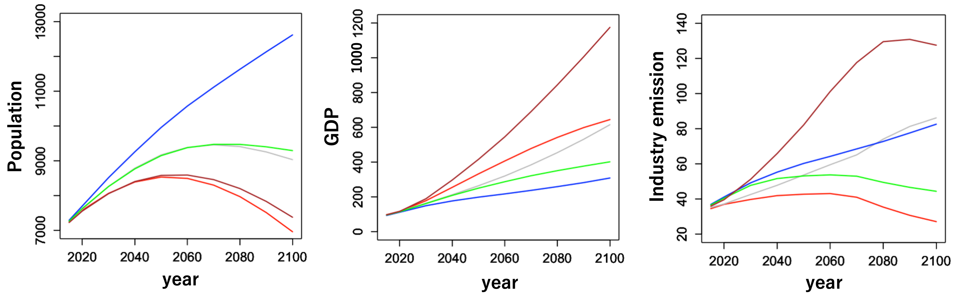
Figure 1: Global population (millions), GDP (trillions 2005 USD per year), and industrial $\mathrm{CO}_{2}$ emission (Gigaton) scenarios by marker SSPs (Red: SSP1, Grey: SSP2, Blue: SSP3, Green: SSP4, Brown: SSP5).

The data are available from the SSPdata-IIASA database. In addition to data from marker SSPs, we also considered data for non-marker SSPs. Not all IAMs can run for all SSPs. For non-marker scenarios, we consider four IAMs: AIM/CGE, GCAM, IMAGE and WITCH-GLOBIOM Emmerling et al. (2016) that have results under all five SSPs.

We use the baseline SSP scenarios from the process-based IAMs to estimate the DICE exogenous functions as follows (the corresponding variables taken from the SSP-IAM scenario are indicated by $\widehat{}$ ).

• The population $L_{t}$ is taken from the SSP-IAM scenario, i.e. $L_{t}=\widehat{L}_{t}$.

• The decarbonisation function $\sigma_{t}$ is estimated as $\sigma_{t}=\widehat{E}^{\mathrm{Ind}}_{t}$/$\widehat{Y}_{t}$, where $\widehat{E}^{\mathrm{Ind}}_{t}$ is taken from the IAM baseline scenarios and $\widehat{Y}_{t}$ is the gross GDP in the baseline SSPs.

• Land emission $E^{\mathrm{Land}}_{t}$ is taken from SSPs, i.e., $E^{\mathrm{Land}}_{t}=\widehat{E}^{\mathrm{Land}}_{t}$.

• The total productivity factor $A_{t}$ is calibrated so that the gross GDP $Y_{t}$ from DICE matches $\widehat{Y}_{t}$ the gross GDP in the baseline SSPs. This calibration involves iterative process described in Yang et al. (2018) that, for each iteration $m=1,2,...$ calculates the DICE trajectories of $Y^{(m)}_{t}$ and model state variables $X^{(m)}_{t}$, $t=0,1,...,N$ using

  $$A^{(m)}_{t}=\frac{\widehat{Y}_{t}}{\big{(}K^{(m-1)}_{t}\big{)}^{\gamma}\widehat{L}_{t}^{1-\gamma}},\;t=0,1,...,N$$ (10)

  until trajectory of $Y^{(m)}_{t}$ approximates the SSP trajectory of $\widehat{Y}_{t}$ closely. Each iteration involves solving the DICE model (optimizing the welfare function with respect to the consumption) without climate damage and abatement costs, $K^{(0)}_{t}$ is taken from the original DICE solution, and convergence is achieved after few iterations.

Then for each baseline SSP and process-based IAM we solve DICE (miximising the welfare function wrt consumption $C_{t}$) resulting in determinstic trajectory for temperature, carbon concentration and social cost of carbon. We do not optimise welfare function in DICE for emission control $\widetilde{\mu}_{t}\in[0,1]$ but we consider scenarios when net-zero emission is achieved by a specific year as follows:

• Net-zero in 2050: $\tilde{\mu}_{t}$ increases linearly from 0 in 2015 to 1 in the year 2050 and remains 1 afterward; and

• Net-zero in 2100: $\tilde{\mu}_{t}$ increases linearly from 0 in 2015 to 1 in the year 2100 and remains 1 afterward.

We also consider emission control scenarios of achieving zero industrial emission:

• zero industrial emission in 2050: $\mu_{t}$ increases linearly from 0 in 2015 to 1 in 2050 and remains 1 afterward; and

• zero industrial emission in 2100: $\mu_{t}$ is increases linearly from 0 in 2015 to 1 in year 2100 and remains 1 afterward.

For comparison, under the original DICE-2016 model, optimal $\mu_{t}$ reaches 1 in 2115. The idea of considering scenarios for greenhouse gas emission $\mu_{t}$ under the DICE framework is not new. For example, it was previously attempted under DICE-2008 in Howarth et al. (2014) and Gerst et al. (2013), where the emission control rate scenario rises from a value of zero in 2010 to unity in the year 2270.

It is important to note that GDP in the SSP database is in 2005 USD year rate while the DICE model assumes 2010 year rate. The SSP’s GDP is converted to the 2010 year rate by multiplying 1.14 that is the corresponding growth rate of the consumer price index (CPI) evaluated by the CPI Inflation Calculator from the US Bureau of Labor Statistics (https://www.bls.gov/data/inflation_calculator.htm). Finally, since SSPs are available only until 2100, to run the DICE model, we project the SSP-IAM population, GDP, and carbon emission scenarios after 2100 using log-linear trend extrapolation method, e.g. see Yamagata et al. (2015).

3 Results

Figure 2 shows the DICE results for the trajectories of atmospheric temperature, atmospheric concentration and social cost of carbon under five SSP markers from 2015 to 2100. Each subplot in Figure 2 shows the trajectory under the original DICE (black dashed line), the trajectory under the scenario of achieving net-zero emissions in 2050 (red line) and the trajectory under the scenario of achieving net-zero emission in 2100 (blue line). Here, the original DICE trajectory is for benchmarking.

As expected we can see that the temperature under the scenario of net-zero in 2050 is lower than under the scenario of net-zero in 2100 across all SSPs. Under the 2050 net-zero scenario, the temperature in 2100 is about 2.5^∘C for all SSPs while under the 2100 net-zero scenario, temperature in 2100 is just under 3^∘C for SSP1 and materially larger than 3^∘C for SSP2-SSP5. This is of course not surprising because SSP1 corresponds to “Green road” scenario. The original DICE trajectory of temperature is close 2100 net-zero scenario. This is somewhat expected because the optimal $\mu_{t}$ under original DICE reaches 1 in 2115 onwards.

Consistently with this behaviour of temperature, the carbon concentration under the 2050 net-zero scenario is always significantly lower than under the 2100 net-zero scenario. Concentration under 2050 net-zero scenario does not vary much across SSPs, while under the 2100 net-zero scenario concentration is the highest under SSP5 and the lowest under SSP1.

Another observation from Figure 2 is that SCC trajectories are very different across SSPs but almost the same between the 2050 and 2100 net-zero scenarios. Under SSP5, SCC is the largest achieving $400 per ton in 2100, about $150 under SSP3 and SSP4, about $250 under SSP2 and about $200 under SSP1. Note that SSP5 is the scenario of “Fossil fueled development” and thus leading to the largest social cost of carbon. In 2025, SCC is approximately $30-50 across SSP markers and close to the original DICE results.

In addition to plots, the temperature results under the marker SSPs for the year 2100 are shown in Table 1. Here, we show results for the net-zero scenarios and zero industrial emission scenarios. There is almost no difference between net-zero and zero industrial emission scenarios. Repeating what we observed in Figure 2, the smallest temperature 2.5^∘C is achieved under SSP1 and net-zero in 2050, and it is larger to 2.6^∘C under other marker SSPs for net zero in 2050. For the 2100 net-zero scenario, SSPs lead to more variation in temperature ranging from 3^∘C under SSP1 to 3.6^∘C under SSP5.

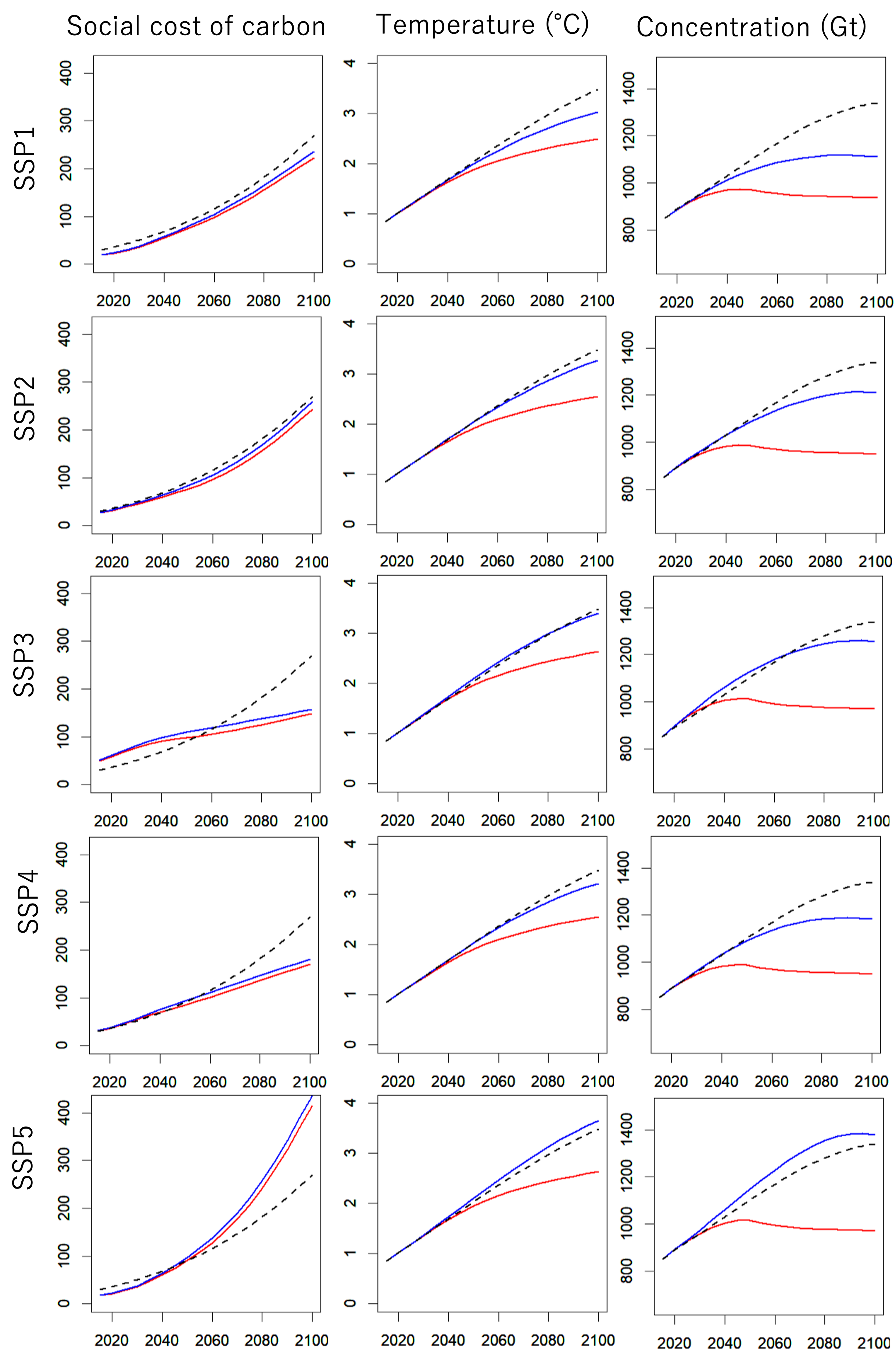
Figure 2: DICE results for social cost of carbon ($SCC_{t}$, $ per ton of $\mathrm{CO}_{2}$), temperature ($T_{t}^{\mathrm{AT}}$), and carbon concentration ($M_{t}^{\mathrm{AT}}$) under five marker SSPs under the scenarios achieving net-zero emissions in 2050 (red) and 2100 (blue). Black dashed line denotes the original DICE model results.

Table 1: Atmospheric temperature $T^{\mathrm{AT}}$ in 2100 under net-zero and zero industry emission mitigation scenarios for marker SSPs.

	SSP1	SSP2	SSP3	SSP4	SSP5
Net-zero in 2050	2.50	2.55	2.63	2.55	2.63
Net-zero in 2100	3.03	3.26	3.40	3.22	3.65
Zero industrial emission in 2050	2.49	2.62	2.75	2.63	2.68
Zero industrial emission in 2100	3.02	3.29	3.45	3.25	3.66

One can also observe that zero industrial emission scenario under marker SSP1 leads to slightly smaller temperature compared to the net-zero scenario. This is because the land-use emission is negative from 2050 under marker SSP1 (i.e. under SSP1-IMAGE) while positive under other marker SSPs. Negative land emission leads to negative total emission for zero industrial emission scenario, while net-zero scenario leads to only zero total emission resulting in the slightly higher temperature under the net-zero scenario.

For non-marker scenarios, we consider four IAMs: AIM/CGE, GCAM, IMAGE and WITCH-GLOBIOM that have results under all five SSPs in the SSPdata-IIASA database. Table 2 shows atmospheric temperature in the year 2100 produced by the DICE model calibrated to the non-marker scenarios. Here, we see results similar to Table 1. Net-zero and zero industry emission scenarios lead to approximately the same results. Under the 2050 net-zero scenario, temperature range is 2.5-2.7^∘C across SSPs and IAMs. Under the 2100 net-zero scenario, temperature range is 3.0-3.7^∘C. We also calculated trajectories of atmospheric temperature, atmospheric concentration and social cost of carbon under non-marker scenarios from 2015 to 2100 presented in Figures 3-6. These results are not materially different from the DICE results under the marker scenarios in Figure 2, confirming the consistency in predictions across considered process-based IAMs.

Table 2: Atmospheric temperature $T^{\mathrm{AT}}$ in 2100 under net-zero and zero industry emission mitigation scenarios for non-marker scenarios: five SSPs under four IAMs (AIM/CGE, GCAM, IMAGE, WITCH-GLOBIOM).

	Net-zero in 2050					Zero industrial emission in 2050
SSP	AIM	GCAM	IMAGE	WITCH		AIM	GCAM	IMAGE	WITCH
1	2.5	2.5	2.5	2.5		2.5	2.4	2.5	2.5
2	2.6	2.6	2.6	2.6		2.7	2.6	2.7	2.6
3	2.6	2.6	2.6	2.6		2.8	2.8	2.8	2.7
4	2.6	2.6	2.5	2.5		2.7	2.6	2.6	2.5
5	2.6	2.6	2.7	2.6		2.7	2.6	2.7	2.7
	Net-zero in 2100					Zero industrial emission in 2100
SSP	AIM	GCAM	IMAGE	WITCH		AIM	GCAM	IMAGE	WITCH
1	3.0	3.1	3.0	3.1		3.0	3.0	3.0	3.1
2	3.3	3.3	3.3	3.3		3.4	3.3	3.3	3.3
3	3.4	3.4	3.3	3.4		3.5	3.5	3.4	3.4
4	3.1	3.2	3.2	3.2		3.2	3.3	3.2	3.2
5	3.5	3.6	3.6	3.6		3.5	3.6	3.7	3.6

4 Conclusions

In this paper we analysed climate-economy trajectories using the cost-benefit DICE model calibrated to five baseline SSPs and six main process-based IAMs. For emission mitigation control, we considered two scenarios: achieving net-zero in 2050 and in 2100. We also considered scenarios of achieving zero industrial emission in 2050 and in 2100.

The main observation is that even if net-zero emission (or zero industrial emission) is achieved by 2050, the temperature will exceed $2^{\circ}\text{C}$ by 2100 (ranging from $2.5^{\circ}\text{C}$ to $2.7^{\circ}\text{C}$) under all five SSPs and six IAMs considered. For more lenient mitigation achieving zero emission by 2100, the temperature will be in the range between $3^{\circ}\text{C}$ and $3.7^{\circ}\text{C}$ by 2100 depending on the SSP-IAM. The social cost of carbon is raising from USD 30-50 in 2025 to USD 250-400 in 2100 depending on SSP-IAM with only very marginal impact from net-zero scenarios. This is generally consistent with other literature, see e.g. Riahi et al. (2022) and Yang et al. (2018) and provides a carbon price benchmark for policy makers. SCC does not depend significantly on the emission mitigation scenario because it measures the marginal damage to the economy from carbon emissions.

As expected, the smallest temperature corresponds to SSP1 and largest to SSP5. Here, we note, that temperature trajectories in Yang et al. (2018) are in the range 3.75-4.5 ^∘C in 2100 across five SSPs higher than in our study because they are calculated for optimal emission reduction $\mu_{t}$ while our results correspond to scenarios for $\mu_{t}$ leading to zero emissions in 2050 and 2100. The results are aligned with the findings in Tol (2023) that the Paris Agreement temperature targets cannot be met without very rapid reduction of greenhouse gas emissions and removal of carbon dioxide from the atmosphere using negative emission technologies Santos et al. (2019). The latter requires perhaps prohibitively large subsidies.

Many sources of uncertainty can be considered in the DICE model, such as uncertainties in the damage function, total productivity growth, or decarbonisation function decline rate that have a significant impact on the future trajectories of climate and economy not considered in our study. These have been studied as parameter uncertainties in Nordhaus (2018). Stochastic versions of DICE where optimal policy is calculated as a decision under uncertainty solving optimal stochastic control problem are also considered in Traeger (2014); Cai and Lontzek (2019); Arandjelović et al. (2024); Shevchenko et al. (2022). Considering stochastic DICE models with exogenous functions calibrated to SSPs should also provide important benchmarks and will be considered in our future studies.

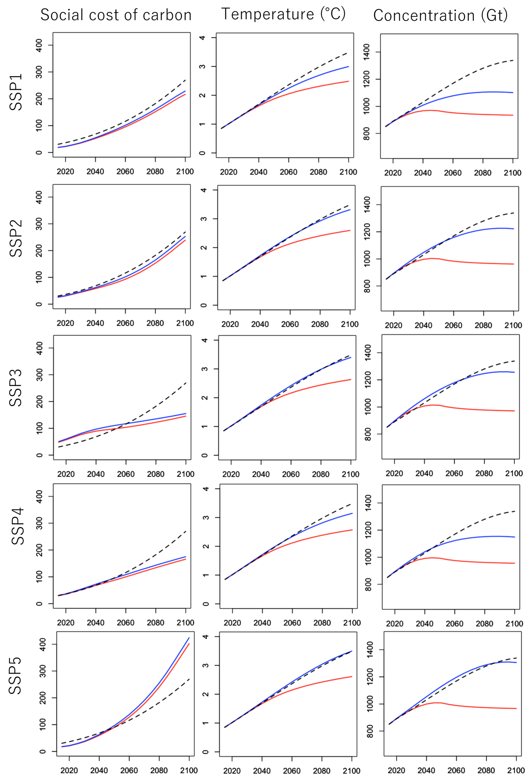
Figure 3: Social cost of carbon ($SCC_{t}$, $ per ton of $\mathrm{CO}_{2}$), temperature ($T_{t}^{\mathrm{AT}}$), and carbon concentration ($M_{t}^{\mathrm{AT}}$) from the DICE model calibrated to baseline SSPs in AIM for scenarios of achieving net-zero emissions in 2050 (red) and 2100 (blue). Black dashed line denotes the original DICE model results.

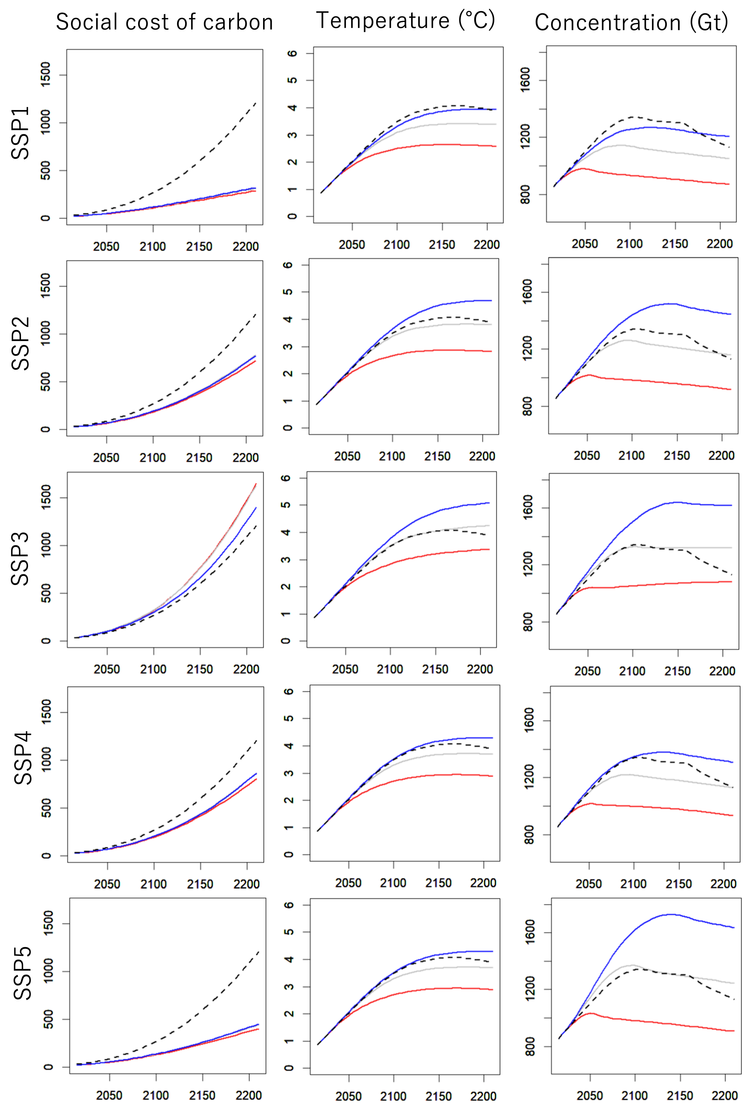
Figure 4: Social cost of carbon ($ per ton of $\mathrm{CO}_{2}$), temperature, and carbon concentration from the DICE model calibrated to baseline SSPs in GCAM for scenarios of achieving net-zero emissions in 2050 (red) and 2100 (blue). Black dashed line denotes the original DICE model results.

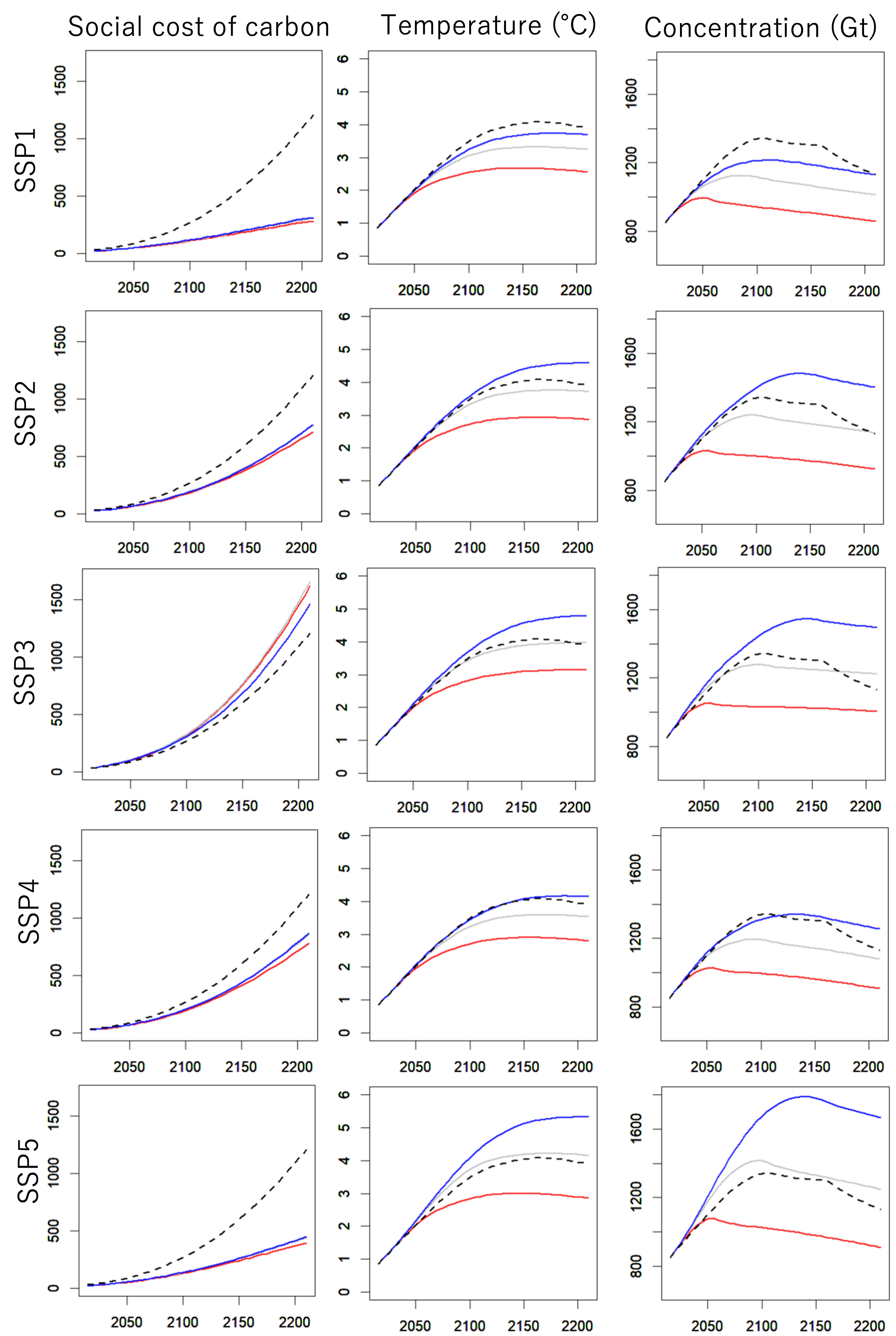
Figure 5: Social cost of carbon ($SCC_{t}$, $ per ton of $\mathrm{CO}_{2}$), temperature ($T_{t}^{\mathrm{AT}}$), and carbon concentration ($M_{t}^{\mathrm{AT}}$) from the DICE model calibrated to baseline SSPs in IMAGE for scenarios of achieving zero emissions in 2050 (red) and 2100 (blue). Black dashed line denotes the original DICE model results.

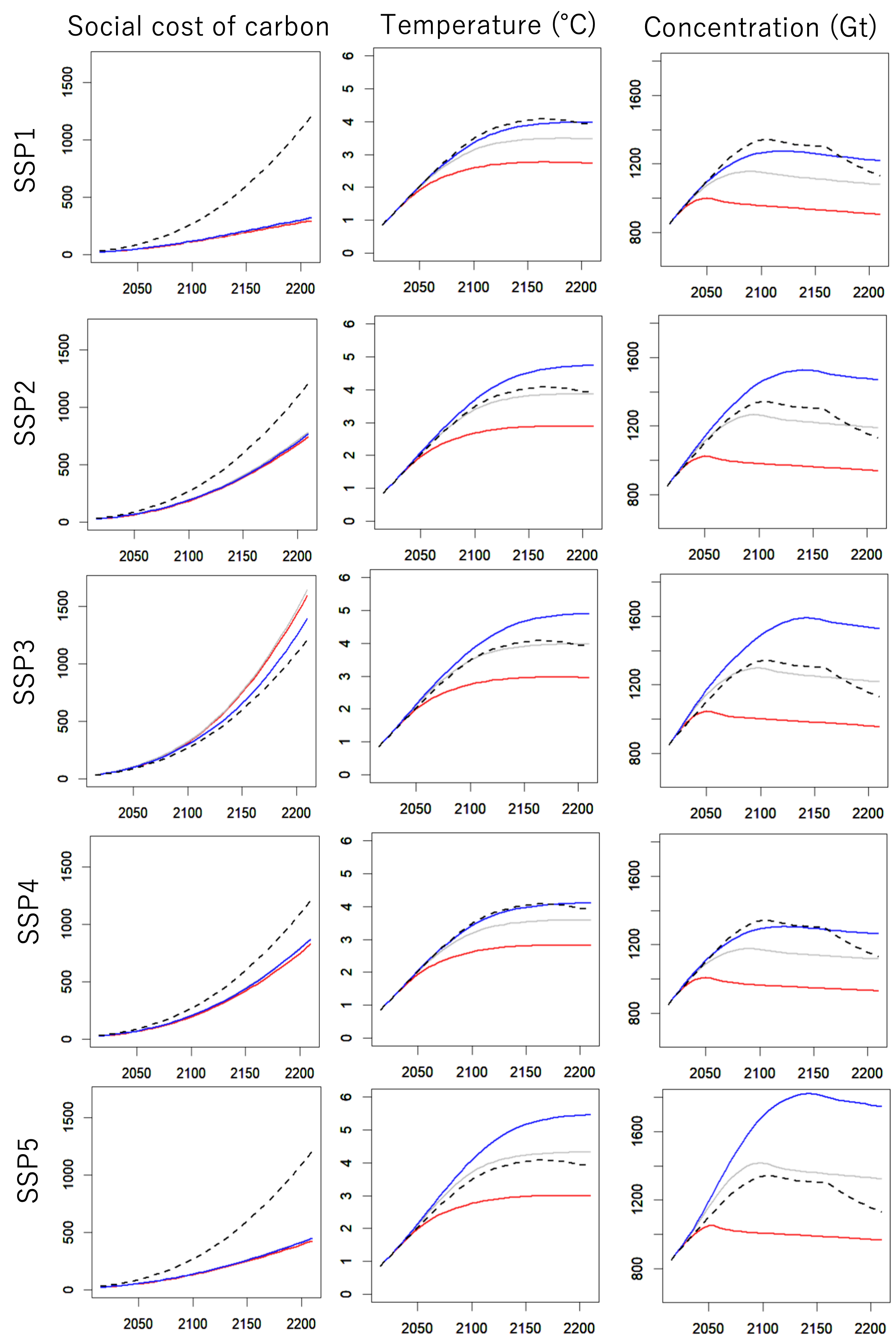
Figure 6: Social cost of carbon ($SCC_{t}$, $ per ton of $\mathrm{CO}_{2}$), temperature ($T_{t}^{\mathrm{AT}}$), and carbon concentration ($M_{t}^{\mathrm{AT}}$) from the DICE model calibrated to baseline SSPs in WITCH-GLOBIOM for scenarios of achieving net-zero emissions in 2050 (red) and 2100 (blue). Black dashed line denotes the original DICE model results.

References

- Anthoff and Tol (2010) Anthoff, D., Tol, R., 2010. The Climate Framework for Uncertainty, Negotiation and Distribution (FUND), Technical Description, Version 3.5. Technical Report. Economic and Social Research Institute, Dublin.
- Arandjelović et al. (2024) Arandjelović, A., Shevchenko, P.V., Matsui, T., Murakami, D., Myrvoll, T.A., 2024. Solving stochastic climate-economy models: A deep least-squares Monte Carlo approach. arXiv preprint arXiv:2408.09642 .
- Bäuerle and Rieder (2011) Bäuerle, N., Rieder, U., 2011. Markov decision processes with applications to finance. Springer Science & Business Media.
- Braun et al. (2024) Braun, P., Faulwasser, T., Grüne, L., Kellett, C.M., Semmler, W., Weller, S.R., 2024. On the social cost of carbon and discounting in the dice model. AIMS Environmental Science 11, 471–495. DOI: 10.3934/environsci.2024024.
- Cai and Lontzek (2019) Cai, Y., Lontzek, T.S., 2019. The social cost of carbon with economic and climate risks. Journal of Political Economy 127, 2684–2734.
- Calvin et al. (2017) Calvin, K., Bond-Lamberty, B., Clarke, L., Edmonds, J., Eom, J., Hartin, C., Kim, S., Kyle, P., Link, R., Moss, R., et al., 2017. The ssp4: A world of deepening inequality. Global Environmental Change 42, 284–296.
- Emmerling et al. (2016) Emmerling, J., Drouet, L., Reis, L.A., Bevione, M., Berger, L., Bosetti, V., Carrara, S., De Cian, E., D’Aertrycke, G.D.M., Longden, T., et al., 2016. The WITCH 2016 model-documentation and implementation of the shared socioeconomic pathways. Technical Report. Nota di Lavoro.
- Fricko et al. (2017) Fricko, O., Havlik, P., Rogelj, J., Klimont, Z., Gusti, M., Johnson, N., Kolp, P., Strubegger, M., Valin, H., Amann, M., et al., 2017. The marker quantification of the shared socioeconomic pathway 2: A middle-of-the-road scenario for the 21st century. Global Environmental Change 42, 251–267.
- Fujimori et al. (2017) Fujimori, S., Hasegawa, T., Masui, T., Takahashi, K., Herran, D.S., Dai, H., Hijioka, Y., Kainuma, M., 2017. Ssp3: Aim implementation of shared socioeconomic pathways. Global Environmental Change 42, 268–283.
- Gerst et al. (2013) Gerst, M.D., Howarth, R.B., Borsuk, M.E., 2013. The interplay between risk attitudes and low probability, high cost outcomes in climate policy analysis. Environmental Modelling & Software 41, 176–184.
- Grubb et al. (2021) Grubb, M., Wieners, C., Yang, P., 2021. Modeling myths: On DICE and dynamic realism in integrated assessment models of climate change mitigation. Wiley Interdisciplinary Reviews: Climate Change 12, e698.
- Hope (2008) Hope, C.W., 2008. Optimal carbon emissions and the social cost of carbon over time under uncertainty. Integrated Assessment Journal 8.
- Howarth et al. (2014) Howarth, R.B., Gerst, M.D., Borsuk, M.E., 2014. Risk mitigation and the social cost of carbon. Global Environmental Change 24, 123–131.
- Interagency Working Group on Social Cost of Greenhouse Gases (2016) Interagency Working Group on Social Cost of Greenhouse Gases, 2016. Technical Support Document: Social Cost of Carbon for Regulatory Impact Analysis Under Executive Order 12866. Technical Report. United States Government.
- Kriegler et al. (2017) Kriegler, E., Bauer, N., Popp, A., Humpenöder, F., Leimbach, M., Strefler, J., Baumstark, L., Bodirsky, B.L., Hilaire, J., Klein, D., et al., 2017. Fossil-fueled development (ssp5): An energy and resource intensive scenario for the 21st century. Global environmental change 42, 297–315.
- Moss et al. (2010) Moss, R.H., Edmonds, J.A., Hibbard, K.A., Manning, M.R., Rose, S.K., Van Vuuren, D.P., Carter, T.R., Emori, S., Kainuma, M., Kram, T., et al., 2010. The next generation of scenarios for climate change research and assessment. Nature 463, 747–756.
- Nordhaus (2014) Nordhaus, W., 2014. Estimates of the social cost of carbon: concepts and results from the dice-2013r model and alternative approaches. Journal of the Association of Environmental and Resource Economists 1, 273–312.
- Nordhaus (2018) Nordhaus, W., 2018. Projections and uncertainties about climate change in an era of minimal climate policies. American Economic Journal: Economic Policy 10, 333–360.
- Nordhaus (2017) Nordhaus, W.D., 2017. Revisiting the social cost of carbon. Proceedings of the National Academy of Sciences 114, 1518–1523.
- Nordhaus et al. (1992) Nordhaus, W.D., et al., 1992. The ‘DICE’ model: background and structure of a dynamic integrated climate-economy model of the economics of global warming. Technical Report. Cowles Foundation for Research in Economics, Yale University.
- Pindyck (2017) Pindyck, R.S., 2017. The use and misuse of models for climate policy. Review of Environmental Economics and Policy 11, 100–114.
- Riahi et al. (2022) Riahi, K., Schaeffer, R., Arango, J., Calvin, K., Guivarch, C., Hasegawa, T., Jiang, K., Kriegler, E., Matthews, R., Peters, G., Rao, A., Robertson, S., Sebbit, A.M., Steinberger, J., Tavoni, M., van Vuuren, D., 2022. Mitigation pathways compatible with long-term goals, in: Shukla, P., Skea, J., Slade, R., Khourdajie, A.A., van Diemen, R., McCollum, D., Pathak, M., S. Some, P.V., R. Fradera, M.B., Hasija, A., Lisboa, G., Luz, S., Malley, J. (Eds.), IPCC, 2022: Climate Change 2022 - Mitigation of Climate Change: Working Group III Contribution to the Sixth Assessment Report of the Intergovernmental Panel on Climate Change. Cambridge University Press, pp. 295–408. doi: 10.1017/9781009157926.005.
- Riahi et al. (2017) Riahi, K., Van Vuuren, D.P., Kriegler, E., Edmonds, J., O’neill, B.C., Fujimori, S., Bauer, N., Calvin, K., Dellink, R., Fricko, O., et al., 2017. The shared socioeconomic pathways and their energy, land use, and greenhouse gas emissions implications: An overview. Global Environmental Change 42, 153–168.
- Santos et al. (2019) Santos, F.M., Gonçalves, A.L., Pires, J.C., 2019. Negative emission technologies, in: Bioenergy with carbon capture and storage. Elsevier. chapter 1, pp. 1–13. https://doi.org/10.1016/B978-0-12-816229-3.00001-6.
- Shevchenko et al. (2022) Shevchenko, P.V., Murakami, D., Matsui, T., Myrvoll, T.A., 2022. Impact of covid-19 type events on the economy and climate under the stochastic DICE model. Environmental Economics and Policy Studies 24, 459–476.
- Tol (2023) Tol, R.S., 2023. Costs and benefits of the paris climate targets. Climate Change Economics 14, 2340003.
- Traeger (2014) Traeger, C.P., 2014. A 4-stated DICE: Quantitatively addressing uncertainty effects in climate change. Environmental and Resource Economics 59, 1–37.
- United Nations Treaty Collection (2015) United Nations Treaty Collection, 2015. Paris Agreement. https://treaties.un.org/pages/ViewDetails.aspx?src=TREATY&mtdsg_no=XXVII-7-d&chapter=27&clang=_en.
- Van Beek et al. (2020) Van Beek, L., Hajer, M., Pelzer, P., van Vuuren, D., Cassen, C., 2020. Anticipating futures through models: the rise of integrated assessment modelling in the climate science-policy interface since 1970. Global Environmental Change 65, 102191.
- Van Vuuren et al. (2012) Van Vuuren, D.P., Riahi, K., Moss, R., Edmonds, J., Thomson, A., Nakicenovic, N., Kram, T., Berkhout, F., Swart, R., Janetos, A., et al., 2012. A proposal for a new scenario framework to support research and assessment in different climate research communities. Global Environmental Change 22, 21–35.
- Van Vuuren et al. (2017) Van Vuuren, D.P., Stehfest, E., Gernaat, D.E., Doelman, J.C., Van den Berg, M., Harmsen, M., de Boer, H.S., Bouwman, L.F., Daioglou, V., Edelenbosch, O.Y., et al., 2017. Energy, land-use and greenhouse gas emissions trajectories under a green growth paradigm. Global Environmental Change 42, 237–250.
- Weyant (2017) Weyant, J., 2017. Some contributions of integrated assessment models of global climate change. Review of Environmental Economics and Policy 11, 115–137.
- Yamagata et al. (2015) Yamagata, Y., Murakami, D., Seya, H., 2015. A comparison of grid-level residential electricity demand scenarios in japan for 2050. Applied Energy 158, 255–262.
- Yang et al. (2018) Yang, P., Yao, Y.F., Mi, Z., Cao, Y.F., Liao, H., Yu, B.Y., Liang, Q.M., Coffman, D., Wei, Y.M., 2018. Social cost of carbon under shared socioeconomic pathways. Global Environmental Change 53, 225–232.