Out-of-equilibrium dynamics across the first-order quantum transitions
of one-dimensional quantum Ising models

Abstract

We study the out-of-equilibrium dynamics of one-dimensional quantum Ising models in a transverse field $g$, driven by a time-dependent longitudinal field $h$ across their magnetic first-order quantum transition at $h=0$, for sufficiently small values of $|g|$. We consider nearest-neighbor Ising chains of size $L$ with periodic boundary conditions. We focus on the out-of-equilibrium behavior arising from Kibble-Zurek protocols, in which $h$ is varied linearly in time with time scale $t_{s}$, i.e., $h(t)=t/t_{s}$. The system starts from the ground state at $h_{i}\equiv h(t_{i})<0$, where the longitudinal magnetization $M$ is negative. Then it evolves unitarily up to positive values of $h(t)$, where $M(t)$ becomes eventually positive. We identify several scaling regimes characterized by a nontrivial interplay between the size $L$ and the time scale $t_{s}$, which can be observed when the system is close to one of the many avoided level crossings that occur for $h\geq 0$. In the $L\to\infty$ limit, all these crossings approach $h=0^{+}$, making the study of the thermodynamic limit, defined as the limit $L\to\infty$ keeping $t$ and $t_{s}$ constant, problematic. We study such limit numerically, by first determining the large-$L$ quantum evolution at fixed $t_{s}$, and then analyzing its behavior with increasing $t_{s}$. Our analysis shows that the system switches from the initial state with $M<0$ to a positively magnetized state at $h=h_{\star}(t_{s})>0$, where $h_{\star}(t_{s})$ decreases with increasing $t_{s}$, apparently as $h_{\star}\sim 1/\ln t_{s}$. This suggests the existence of a scaling behavior in terms of the rescaled time $\Omega=t\ln t_{s}/t_{s}$. The numerical results also show that the system converges to a nontrivial stationary state in the large-$t$ limit, characterized by an energy significantly larger than that of the corresponding homogeneously magnetized ground state.

I Introduction

Out-of-equilibrium phenomena at first-order phase transitions have been much investigated both in classical statistical models (see the reviews Binder-87 ; PV-24 and, e.g., Refs. NN-75 ; FB-82 ; PF-83 ; FP-85 ; CLB-86 ; BK-90 ; LK-91 ; BK-92 ; VRSB-93 ; MM-00 ; LFGC-09 ; NIW-11 ; TB-12 ; ICA-14 ; PV-15 ; PV-16 ; PV-17 ; PV-17-dyn ; LZ-17 ; PPV-18 ; Fontana-19 ; CCP-21 ; CCEMP-22 ) and in quantum many-body systems at zero temperature (see the reviews Pfleiderer-05 ; RV-21 ; PV-24 and, e.g., Refs. AC-09 ; YKS-10 ; JLSZ-10 ; LMSS-12 ; CNPV-14 ; CNPV-15 ; CPV-15 ; CPV-15-iswb ; PRV-18 ; PRV-18-fowb ; YCDS-18 ; RV-18 ; PRV-18-def ; SW-18 ; LZW-19 ; PRV-20 ; DRV-20 ; SCD-21 ; TV-22 ; TS-23 ). Since first-order transitions appear in several different physical contexts, any progress in the theoretical understanding of related nonequilibrium phenomena is of great phenomenological importance. The condensation of water, the melting of ice, etc., are some examples of first-order classical transitions at finite temperature. First-order transitions driven by quantum fluctuations occur in quantum Hall systems PPBWJ-99 , itinerant ferromagnets VBKN-99 ; BKV-99 , heavy fermion metals UPH-04 ; Pfleiderer-05 ; KRLF-09 , SU($N$) magnets DK-16 ; DK-20 , quantum spin systems LMSS-12 ; CNPV-14 ; LZW-19 , etc. They display notable equilibrium and out-of-equilibrium scaling behaviors, like classical and quantum continuous transitions (see, e.g., Refs. Fisher-74 ; Wilson-83 ; ZJ-book ; PV-02 ; Sachdev-book ; CPV-14 ; RV-21 ). In particular, classical and quantum systems at first-order transitions turn out to be particularly sensitive to the boundary conditions. Actually, the sensitivity of the large-distance or low-energy properties to the boundary conditions is one of the main distinctive differences between the behaviors of finite-size systems at continuous and first-order transitions PV-24 .

In this paper we discuss the dynamics of one-dimensional quantum Ising models in a transverse field, driven by a time-varying longitudinal homogeneous field $h$ across the magnetic first-order quantum transition (FOQT) at $h=0$. We consider periodic boundary conditions, which preserve the ${\mathbb{Z}}_{2}$ symmetry of the model at $h=0$. Moreover, they preserve translational invariance, which allows us to focus on translation-invariant states, significantly simplifying the numerical analysis. We investigate the out-of-equilibrium behavior arising from Kibble-Zurek (KZ) protocols, in which $h$ varies linearly with time with time scale $t_{s}$, i.e., $h(t)=t/t_{s}$. The system starts from the negatively magnetized ground state at $h_{i}\equiv h(t_{i})<0$, and then evolves unitarily up to a positive value $h(t)$, eventually leading to states with positive longitudinal magnetization.

In the KZ dynamics, the time-dependent observables monitoring the system develop an out-of-equilibrium finite-size scaling (OFSS) behavior PV-24 ; RV-21 ; PRV-18 ; PRV-18-fowb ; RV-18 ; PRV-20 ; TV-22 ; TS-23 when $t_{s}\sim T(L)$, where $T(L)$ is the typical time it takes the system to make a transition from a magnetized state to the opposite one. The time scale $T(L)$ is related to the exponentially small gap $\Delta\sim e^{-bL}$ at $h=0$, i.e., $T(L)\sim L/\Delta^{2}$. Thus, $T(L)\sim e^{2bL}$ (apart from powers of $L$) increases very rapidly with the system size. When $t_{s}\gg T(L)$, the system evolves adiabatically for $h\approx 0$, switching from the negatively magnetized ground state to the positive one. On the other hand, for $t_{s}\ll T(L)$, the passage through the $h=0$ avoided level crossing is effectively instantaneous, so the system persists in the wrongly magnetized state ($M<0$) for $h(t)>0$, as in the analogous Landau-Zener problem for two-level systems Landau-32 ; Zener-32 ; VG-96 . Therefore, the OFSS for $h\approx 0$ can be observed only for relatively small systems or very large time scales $t_{s}$ RV-21 ; PV-24 .

Beside the avoided level crossing at $h=0$, the low-energy spectrum of finite-size systems shows a sequence of avoided level crossings between the ${\rm wrongly}$ magnetized state and a discrete series of zero-momentum kink-antikink states, labeled by $k=1,2,\ldots$. We can associate a time scale $T_{k}(L)$ with each crossing, which is relevant for the dynamics of the system when $t_{s}\ll T(L)$. Since, the time scales satisfy $T(L)\gg T_{1}(L)\gg T_{2}(L)\gg\ldots$, the time scale $t_{s}$ can be tuned in such a way to select at which avoided crossing the system magnetization changes sign. More precisely, for $t_{s}\ll T(L)$, the negatively magnetized state effectively survives across the $h=0$ and the first $k-1$ avoided level crossings up to the one satisfying $t_{s}\approx T_{k}(L)$. When $h(t)\approx h_{k}(L)$, the system jumps to a kink-antikink state with positive magnetization. A similar behavior was also observed in Ref. SCD-21 .

Since, the additional avoided crossings are localized at $h_{k}(L)=a/L+a_{1k}/L^{5/3}+O(L^{-2})$, they all collapse to $h=0^{+}$, for $L\to\infty$. Thus, their role in the thermodynamic limit, defined as the limit $L\to\infty$ keeping $t$ and $t_{s}$ constant, becomes unclear and likely irrelevant. We study such thermodynamic limit numerically, by first determining the large-$L$ quantum evolution at fixed $t_{s}$, and then analyzing the behavior with increasing $t_{s}$. As we shall see, our results unveil the emergence of a peculiar infinite-size scaling behavior. We observe that the negatively magnetized state jumps to states with positive magnetization at values $h_{\star}(t_{s})>0$ that approach $h=0$ with increasing $t_{s}$, apparently as $h_{\star}(t_{s})\sim 1/\ln t_{s}$. This suggests an infinite-size scaling behavior in terms of the scaling variable $\Omega=t\ln t_{s}/t_{s}$. Another notable feature of the dynamics is that the quantum Ising system approaches a nontrivial stationary state in the large-$t$ limit, characterized by an energy significantly larger than that of the corresponding magnetized ground state. This difference is related to the average work done to vary the field in the KZ protocol.

The paper is organized as follows. In Sec. II we present the quantum Ising chain and discuss its low-energy spectrum along the FOQT line. In particular, we discuss the small-$h$ behavior of the energy of the lowest kink-antikink bound states, characterized by nonanalytic $h^{2/3}$ corrections. We also identify a sequence of avoided crossings between kink-antikink states and the wrongly magnetized state, which plays a major role in the finite-size KZ dynamics. In Sec. III we discuss the equilibrium finite-size scaling close to such avoided level crossings. In Sec. IV we outline the KZ protocol, while in Sec. V we analyze the OFSS behavior for $h(t)\approx 0$. In Sec. VI we extend the previous discussion to the avoided level crossings that occur for $h>0$. The KZ dynamics in the infinite-size limit is numerically investigated in Sec. VII. In Sec. VIII we summarize and draw our conclusions. Finally, App. A reports some analytical computations of the spectrum of the relevant kink-antikink bound states at small transverse and longitudinal external fields.

II First-order quantum transitions in quantum Ising chains

II.1 The model

The nearest-neighbor quantum Ising chain in a transverse field is a paradigmatic model showing continuous and FOQTs. Its Hamiltonian reads

$$H_{\rm Is}=-J\,\sum_{\langle x,y\rangle}\sigma^{(1)}_{x}\sigma^{(1)}_{y}-g\,\sum_{x}\sigma^{(3)}_{x}-h\,\sum_{x}\sigma^{(1)}_{x},$$ (1)

where $\sigma^{(k)}$ are the spin-$1/2$ Pauli matrices ($k=1,2,3$), the first sum is over all nearest-neighbor bonds $\langle x,y\rangle$, while the second and the third sums are over the $L$ sites of the chain. The Hamiltonian parameters $g$ and $h$ represent homogeneous transverse and longitudinal fields, respectively. Without loss of generality, we assume $J=1$, $g>0$. We also set the Planck constant $\hslash=1$.

At zero temperature, and for $g=1$, $h=0$, the model (1) undergoes a continuous quantum transition belonging to the two-dimensional Ising universality class, separating a disordered phase ($g>1$) from an ordered ($g<1$) one. For any $g<1$, the longitudinal field $h$ drives FOQTs along the $h=0$ line.

The low-energy properties at FOQTs crucially depend on the boundary conditions, even in the $L\to\infty$ limit (see, e.g., Refs. CNPV-14 ; CNPV-15 ; CPV-15 ; CPV-15-iswb ; PRV-18-fowb ; LMSS-12 ; RV-21 ; PV-24 ). We consider periodic boundary conditions, preserving the ${\mathbb{Z}}_{2}$ symmetry and translational invariance. The lowest energy levels for any $g<1$ and $h=0$ are the magnetized states $|+\rangle$ and $|-\rangle$ along the longitudinal direction, which spontaneously break the ${\mathbb{Z}}_{2}$ symmetry in the thermodynamic limit. When varying $h$ across one of the FOQT transition points ($h=0$, $g<1$), their (avoided) level crossing gives rise to a discontinuity in the longitudinal magnetization of the ground state $|\Psi_{0}\rangle$,

$$M={1\over L}\langle\Psi_{0}|\sum_{x}\sigma_{x}^{(1)}|\Psi_{0}\rangle,$$ (2)

in the thermodynamic limit Pfeuty-70 :

$$\lim_{h\to 0^{\pm}}\lim_{L\to\infty}M=\pm\,m_{0},\qquad m_{0}=(1-g^{2})^{1/8}.$$ (3)

II.2 The spectrum

In a finite system of size $L$ with periodic boundary conditions, quantum tunneling effects lift the degeneracy of the two lowest magnetized states, which is present for $h=0$. The Hamiltonian eigenstates are superpositions of the magnetized $|\pm\rangle$ states,

$$|0\rangle={1\over\sqrt{2}}\left(|+\rangle+|-\rangle\right),\qquad|1\rangle={1\over\sqrt{2}}\left(|+\rangle-|-\rangle\right).$$ (4)

Their energy difference

$$\Delta(L)\equiv E_{1}(L)-E_{0}(L)$$ (5)

vanishes exponentially as $L$ increases. Indeed, its asymptotic large-$L$ behavior is given by Pfeuty-70 ; CJ-87

$$\Delta(L)\approx{2\over\sqrt{\pi L}}\,g^{L}.$$ (6)

The differences $E_{n}(L)-E_{0}(L)$ at the transition point $h=0$, between the higher excited states ($n>1$) and the ground state, approach instead finite values for $L\to\infty$. We also recall that the size dependence of the energy difference $\Delta(L)$ between the lowest levels may drastically change when considering other boundary conditions CNPV-14 ; RV-21 ; PV-24 . For example, in the case of antiperiodic and opposite fixed boundary conditions, where the lowest levels are single-kink configurations, the gap $\Delta(L)$ decays as $L^{-2}$ along the FOQT line, for any $g<1$ (see, e.g., Refs. CNPV-14 ; CPV-15-iswb ).

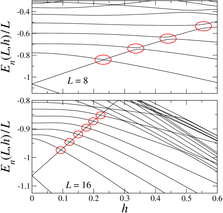
Figure 1: Spectrum of the quantum Ising chain (1) with periodic boundary conditions at zero momentum, as a function of the longitudinal field $h$. Here and in all following figures, we set $g=0.5$. We plot the energy levels $E_{n}(L,h)$ as a function of $h$, for $L=8$ (top) and $L=16$ (bottom). Red circles denote the avoided crossings involving the magnetized state $|-\rangle$ and the lowest-energy zero-momentum kink-antikink states. Data are shown for $h\geq 0$, since the ${\mathbb{Z}}_{2}$ symmetry of the model implies that the spectrum is invariant under $h\to-h$. For the sake of clarity, in the bottom panel we report only the first 20 energy levels.

As for the excitation spectrum, we first recall that periodic boundary conditions preserve translational invariance, implying momentum conservation even in finite systems. This allows us to restrict our analysis of the spectrum to the zero-momentum states, the only ones that are relevant also in dynamic processes preserving translational invariance, i.e., when the initial condition and the external field driving the dynamics are homogeneous. Since the spectrum is symmetric with respect to sign changes of the longitudinal field, i.e., under $h\to-h$, it is sufficient to consider only nonnegative values ($h\geq 0$).

For sufficiently small values of $h$, the relevant low-energy states, beside the magnetized $|\pm\rangle$ states, are zero-momentum superpositions of states like

$$|k_{w}\rangle=|\cdots\uparrow_{x-1}\>\uparrow_{x}\>\downarrow_{x+1}\>\downarrow_{x+2}\cdots\downarrow_{x+w}\>\uparrow_{x+w+1}\cdots\rangle,$$ (7)

which may be interpreted as kink-antikink bound states. Results for their energies in the presence of small longitudinal and transverse fields can be found in Refs. MW-78 ; Rutkevich-08 ; Coldea-etal-10 ; Rutkevich-10 . In App. A we reanalyze the problem, obtaining exact finite-size results for their energy and magnetization. These results allow us to determine the pattern of the locations of the avoided level crossings that characterize the low-energy spectrum of the quantum Ising chain along the FOQT line. Notice that the classification of the low-energy Hamiltonian eigenstates in terms of kink-antikink states is valid only if the magnetic energy $hL$ is small enough, so that the states with no kinks, with one kink and one antikink, with two kinks and two antikinks, etc, are separated in the spectrum. For $g=0$, the separation of these classes of states is $4J$, so this requirement implies $hL\ll 4J$, i.e., $h\ll 4/L$ for $J=1$ and small values of $g$.

We supplement the above-mentioned analytic results with numerical analyses of the spectrum of the quantum Ising chain (1) for $g=1/2$. For this purpose, since the Ising-chain Hamiltonian is nonintegrable for any $h\neq 0$, we use exact diagonalization methods. Lanczos-based techniques allow us to compute the exact representation of the first low-lying zero-momentum eigenstates, for sizes up to $L\sim 26$ in the relevant Hilbert subspace, which has a dimension of approximately $2.6\times 10^{6}$ Sandvik-10 .

In Fig. 1 we show the zero-momentum energy levels for $g=1/2$, as a function of $h$ and for two different sizes $L$, as obtained by exact diagonalization. We note the presence of several avoided crossings. The first one at $h=0$ has been discussed above. The degeneracy of the magnetized states $|\pm\rangle$ at $h=0$, is lifted for finite $L$, with an exponentially small gap, Eq. (6). Other avoided level crossings occur for $h>0$ (red circles), involving the wrongly magnetized state $|-\rangle$ and the kink-antikink states. As it occurs for $h=0$, for finite values of $L$ the degeneracy is lifted with an exponentially small energy gap in the large-$L$ limit. To specify the location of the avoided level crossings, we determine the size-dependent longitudinal field $h_{k}(L)>0$ where the difference between the energies of the $k$th kink-antikink state and of the magnetized state $|-\rangle$ takes its minimim value $\Delta_{m,k}(L)$:

$$\Delta_{m,k}(L)=\mathop{\rm min}_{h}\,[E_{k}(L)-E_{-}(L)],\quad k=1,2,\ldots,\;$$ (8)

As $L$ increases, this quantity behaves as $\Delta_{m,k}\sim e^{-b_{k}L}$, see Fig. 2. A numerical analysis of the data shows that, for a fixed value of $L$, the gap $\Delta_{m,k}(L)$ increases with $k$, at least for the first few values of $k$; moreover, it always satisfies $\Delta_{m,k}(L)>\Delta(L)$, where $\Delta(L)$ is the gap between the lowest states at $h=0$. Indeed, a fit of our numerical results (the colored data sets in Fig 2) with $18\leq L\leq 26$ to the Ansatz

$$\ln\Delta_{m,k}=c_{k}-b_{k}\,L\,,$$ (9)

gives $b_{1}\approx 0.506$, $b_{2}\approx 0.458$, $b_{3}\approx 0.416$, which decrease with $k$ and are always smaller than $b\approx 0.693$, the decay rate of the $h=0$ ground-state gap, obtained from Eq. (6) with $g=1/2$.

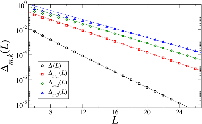
Figure 2: Exact-diagonalization results for the minimum energy differences $\Delta_{m,k}(L)$ between the magnetized state $|-\rangle$ and the first three zero-momentum kink-antikink states (colored data sets), as a function of the lattice size $L$. We also show the energy gap $\Delta(L)$ of the lowest magnetized states at the integrable point $h=0$ (in this case we only considered sizes up to $L=24$, so that $\Delta(L)>10^{-8}$, ensuring numerical convergence of our data). The dashed lines are the results of fits of the data for the largest chain sizes, typically for $L\geq 18$.

The data for the zero-momentum spectrum in Fig. 1 also show that the positions $h_{k}(L)$ of the avoided crossings approach $h=0$ approximately as $h_{k}(L)\sim 1/L$ with increasing $L$. This statement can be justified more rigorously for small values of $g$, by using the exact results (see App. A and Refs. MW-78 ; Rutkevich-08 ; Coldea-etal-10 ; Rutkevich-10 ) obtained in the perturbative $g$ limit. For sufficiently small values of $h$, the energy of the magnetized state $|-\rangle$ can be written as

$$E_{-}(L,h)\approx E_{-}(L,0)+m_{0}\,hL\,.$$ (10)

On the other hand, the energy of the zero-momentum kink-antikink states is (see App. A.2)

$$E_{k}(L,h)=E_{k}(L,0)-m_{0}\,hL+e_{k}\,g^{1/3}h^{2/3}+O(h),\;$$ (11)

where $k=1,2,\ldots$ labels the discrete levels, and the coefficient $e_{k}>0$ increases with increasing $k$. As discussed in App. A.2, the expansion (11) holds when $h$ is small, but still satisfies $h\gg g/L^{3}$, and, in particular, in the finite-size limit $h\to 0$, $L\to\infty$, at fixed (but not too large, as discussed above) $hL$. Subleading corrections (for fixed values of $hL$) decay as $h^{m/3}$, with $m$ integer. The coefficient $e_{k}$ can be exactly computed: $e_{k}=2|\alpha_{k}|$, where $\alpha_{k}<0$ is the $k$th zero of the Airy function. Moreover, we have $m_{0}=1$, as it also occurs for the energy of $|-\rangle$, cf. Eq. (10). Therefore, the relevant kink states are fully magnetized for large values of $L$, as discussed in App. A.3. Equation (11) has been derived for small values of $g$.

We conjecture that a similar expansion holds for all values of $g<1$ in the finite-size limit $h\to 0$, $L\to\infty$, at fixed $hL$. Namely, we assume

$$E_{k}(L,h) = E_{k}(L,0)-m_{0}hL$$ (12)

$$+g^{1/3}h^{2/3}\Bigl{(}e_{k}+\sum_{m=1}^{\infty}e_{k,m}\,h^{m/3}\Bigr{)},\quad$$

where $e_{k}$ and $e_{k,m}$ are functions of $g$ and of $hL$, and the prefactor $g^{1/3}$ has been added for consistency with Eq. (11). Eq. (12) also predicts the behavior of the magnetization of the kink states, since

$$M_{k}(L,h) = -{1\over L}{\partial E_{k}\over\partial h}$$ (13)

$$= m_{0}-{1\over 3L}\left({g\over h}\right)^{1/3}\sum_{m=0}^{\infty}(m+2)e_{k,m},\quad$$

where $e_{k,0}=e_{k}$. Note that the correction term is of order $h^{-1/3}L=1/(hL^{3})^{1/3}$, which is small for $hL^{3}\gg 1$, the regime in which Eqs. (12) and (13) apply.

The location $h_{k}(L)$ of the (avoided) level crossing between the negatively magnetized state and the $k$th kink-antikink state can be obtained by equating the energies

$$E_{-}(L,h_{k})=E_{k}(L,h_{k}).$$ (14)

Note that, for $h=0$, the difference

$$E_{k}(L,0)-E_{-}(L,0)=4+O(g)>0$$ (15)

is finite in the large-$L$ limit and it is independent of $k$, since the energy separation of the zero-momentum kink-antikink states vanishes as $1/L^{2}$ for $h=0$ (see Eq. (58) for $g$ small). Therefore, at leading order, we obtain

$$h_{k}(L)={a\over L},\qquad a={E_{k}(L,0)-E_{-}(L,0)\over 2m_{0}},$$ (16)

where $a$ is independent of $k$. Thus, the avoided crossings occur for values of the magnetic field $h$, where the expansion (12) holds. Solving it perturbatively, we obtain the asymptotic expansion

$$h_{k}(L)={a\over L}+\frac{a_{k}}{L^{5/3}}+\frac{a_{2k}}{L^{2}}+\frac{a_{3k}}{L^{7/3}}+\ldots\,,$$ (17)

with $a_{k}=g^{1/3}e_{k}a^{2/3}/(2m_{0})$. Eq. (17) implies that the difference of the locations of two different level crossings is of order $L^{-5/3}$; more precisely, it behaves as

$$h_{k^{\prime}}(L)-h_{k}(L)={a_{1,kk^{\prime}}\over L^{5/3}}+{a_{2,kk^{\prime}}\over L^{2}}+{a_{3,kk^{\prime}}\over L^{7/3}}+\ldots\,.$$ (18)

Of course, this analysis neglects the interaction terms that cause the crossings to be avoided for finite sizes. However, the region where the avoided level crossing takes place is exponentially small for sufficiently large $L$, so Eq. (17) can be applied to the positions of the avoided crossings, defined by considering the minimum of the energy difference between the two levels.

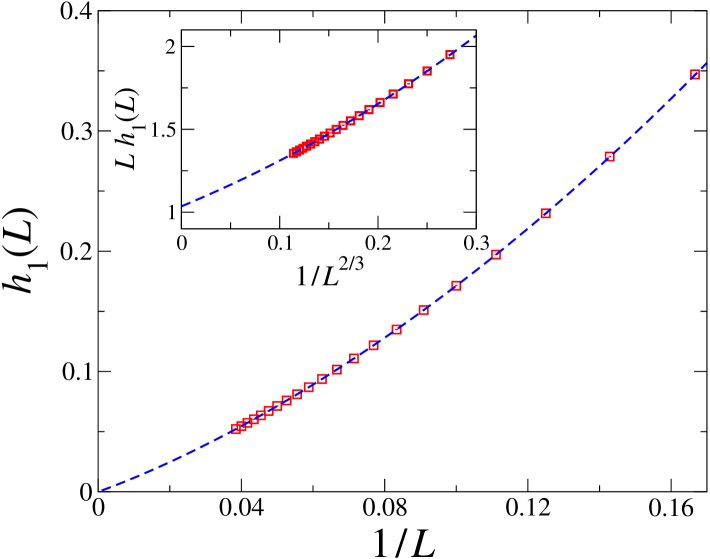
Figure 3: Location $h_{1}(L)$ of the level crossing between the negatively magnetized state and the lowest-energy kink-antikink state as a function of the inverse size $1/L$. The absolute precision of the estimates of $h_{1}(L)$ is approximately $10^{-6}$ for $L\leq 11$, $10^{-7}$ for $12\leq L\leq 15$, and $10^{-9}$ for $16\leq L\leq 26$. The errors are too small to be visible in the figure. The dashed line corresponds to the curve obtained by a four-parameter fit of the data for sizes $L\geq 19$ ($\chi^{2}/{\rm d.o.f}\approx 0.5$) to the expansion (17), see also the text. The inset shows a plot of $L\,h_{1}(L)$ versus $L^{-2/3}$, to highlight the predicted $L^{-2/3}$ subleading behavior, see Eq. (17).

The asymptotic large-$L$ predictions in Eqs. (17) and (18) are supported by the analysis of the numerical data for $g=1/2$. In Fig. 3 we plot the available data for $h_{1}(L)$, the value of $h$ where $E_{1}(L)-E_{-}(L)$ takes its minimum, up to $L=26$. Fits to the Ansatz (17) with four free parameters including only data with $L\geq L_{\rm min}$ give results which are barely dependent on $L_{\rm min}$. In particular, for $L_{\rm min}=19$ (we include the 8 largest sizes) we obtain $a=1.0352(1)$, $a_{1}=2.521(4)$, $a_{21}=-0.50(1)$, and $a_{31}=3.97(2)$ with $\chi^{2}/{\rm d.o.f}\approx 0.5$. The corresponding curve is displayed in dashed blue color.

As discussed in Ref. PRV-18-fowb , in the case of fixed parallel boundary conditions the location of the avoided crossing between the magnetized and lowest-energy kink-antikink state also has an expansion as reported in Eq. (17). Moreover, as discussed in App. A.4, the coefficient $a$ of the $1/L$ term should be the same as for periodic boundary conditions. This is confirmed by our results. The estimate $a\approx 1.0352$ obtained here for periodic boundary conditions is substantially consistent with the result $a=1.0370(5)$ reported in Ref. PRV-18-fowb for fixed parallel boundary conditions. We may also compare the estimate of $a_{1}$ with the small-$g$ approximation $a_{1}\approx e_{1}g^{1/3}a^{2/3}/(2m_{0})$ with $e_{1}=2|\alpha_{1}|$ ($\alpha_{1}$ is the smallest zero of the Airy function, $|\alpha_{1}|\approx 2.338$), see Eq. (77). We obtain $a_{1}\approx 1.97$ for $g=1/2$ (using $a\approx 1.035$ and $m_{0}\approx 0.96$), which is reasonably close to the actual estimate $a_{1}\approx 2.52$ obtained by the fit of our data for $g=1/2$.

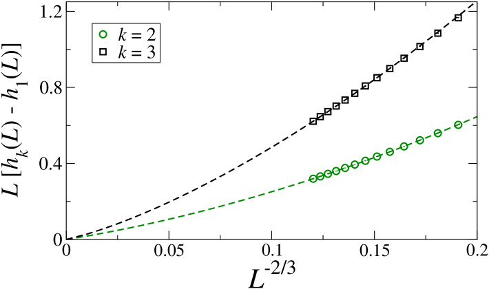
Figure 4: Plot of $L[h_{k}(L)-h_{1}(L)]$ versus $L^{-2/3}$, to highlight the expected behavior $h_{k}(L)-h_{1}(L)\sim L^{-5/3}$. The precision of the estimates of $h_{k}(L)$ with $k=2,3$ is approximately $10^{-6}$ for $L\leq 11$ and $10^{-7}$ for $L\geq 12$.

Finally, in Fig. 4 we show the differences $h_{k}(L)-h_{1}(L)$ for $k=2$ and $k=3$, up to $L=24$. Their behavior is consistent with the asymptotic formula (18). Three-parameter fits to that expansion give $a_{1,12}=1.65(1)$ (using data for $19\leq L\leq 24$, with $\chi^{2}/{\rm d.o.f.}\approx 0.6$) and $a_{1,13}=1.98(4)$ (using data for $L\geq 21$, with $\chi^{2}/{\rm d.o.f.}\approx 0.6$).

III Equilibrium finite-size scaling at the avoided level crossings

At FOQTs the low-energy properties satisfy general equilibrium finite-size scaling (EFSS) laws as a function of the field $h$ and of the system size $L$ CNPV-14 ; PRV-18-fowb ; CNPV-15 ; PV-24 . In the EFSS framework, when the boundary conditions preserve the $h\to-h$ symmetry, the relevant scaling variable is the ratio CNPV-14

$$\Phi={\delta E(L,h)\over\Delta(L)}={2m_{0}hL\over\Delta(L)},$$ (19)

where $\delta E(L,h)=E(L,h)-E(L,-h)=2m_{0}hL$ is the energy difference of the magnetized state when changing the sign of $h$ for small $h$, which quantifies the magnetic energy due to addition of the longitudinal field $h$, while $\Delta(L)\equiv\Delta(L,h=0)$ in the denominator is the ground-state energy gap at $h=0$. The zero-temperature EFSS limit corresponds to $L\to\infty$ and $h\to 0$, keeping $\Phi$ fixed. In this limit, the ground-state magnetization $M(L,h)$ and the energy difference $\Delta(L,h)$ of the lowest levels asymptotically behave as CNPV-14

$$M(L,h)\approx m_{0}\,{\cal M}(\Phi)\,,\quad\Delta(L,h)\approx\Delta(L)\,{\cal D}(\Phi)\,.$$ (20)

An analogous EFSS behavior is expected for other observables, such as the ground-state fidelity RV-18 , and at finite temperature RV-21 .

Unlike continuous quantum transitions, the EFSS at FOQTs drastically depends on the nature of the boundary conditions CNPV-14 ; PRV-18 ; PRV-18-fowb ; RV-21 ; PV-24 . In particular, this is evident when the scaling variable $\Phi$ is expressed in terms of $L$ and $h$, given that the size behavior of $\Delta(L)$ at the FOQT crucially depends on the boundary conditions. Indeed, as already mentioned, the gap $\Delta$ may have either an exponential or a power dependence on $L$, depending on the boundary conditions, although in all cases the finite-size structure of the low-energy spectrum must lead to the discontinuous equilibrium behavior characterizing the FOQTs in the thermodynamic limit. On the opposite side, in continuous quantum transitions the critical power behavior cannot be changed by the boundary conditions.

With neutral boundary conditions, such as periodic boundary conditions, the magnetized states $|\pm\rangle$ represent the lowest-energy excitations. As discussed in Sec. II.2, $\Delta(L)\sim e^{-bL}$ at the FOQT point, while the energy differences $\Delta_{n}\equiv E_{n}-E_{0}$ associated with the higher excited states ($n>1$) are finite (more generally, $\Delta/\Delta_{n}$ decreases exponentially, with possible power corrections) in the large-$L$ limit. For sufficiently large $L$ and $h\ll 1$, the low-energy properties close to the avoided level crossing can be obtained by restricting the theory to the two lowest-energy states $|0\rangle$ and $|1\rangle$, or equivalently to the magnetized states $|+\rangle$ and $|-\rangle$ CNPV-14 ; PRV-18 . In this restricted Hilbert space, the lowest two-level spectrum can be effectively described by a two-level Hamiltonian

$$H_{2{\rm lev}}=\varepsilon\,\sigma^{(3)}+\zeta\,\sigma^{(1)},$$ (21)

where the parameters correspond to $\varepsilon=m_{0}hL$ and $\zeta=\Delta(L)/2$. This effective two-level reduction allows us to exactly compute the EFSS functions of the magnetization $M(L,h)$ and gap $\Delta(L,h)$ CNPV-14 . The convergence to the asymptotic two-level EFSS behavior is generally fast, being controlled by the ratio between the exponentially suppressed gap $\Delta$ and the energy-level differences with the higher states, which are finite for $L\to\infty$.

We remark that the above two-level EFSS behavior arises because only two states, the magnetized states $|\pm\rangle$, are degenerate in the infinite-volume limit at $h=0$. A different behavior emerges in other cases, as for antiperiodic boundary conditions. Indeed, in that situation, an infinite number of states (the single-kink states) become degenerate in the infinite-volume limit. The presence of this infinite tower of degenerate states changes the size behavior of $\Delta(L)$, that scales as $1/L^{2}$ and not exponentially in $L$. Thus, the scaling behavior (20) in terms of the variable $\Phi$ defined in Eq. (19) still holds, but a two-level description of the scaling behavior is no longer valid (see, e.g., Refs. CNPV-14 ; PRV-18-fowb ; RV-21 ; PV-24 ).

The two-level truncation and the corresponding scaling behavior relies on a single basic assumption, that the energy difference $\Delta(L)$ between the two considered states vanishes in the large-$L$ limit faster than the energy differences $\Delta_{n}(L)$ with the neglected states, i.e., $\Delta(L)/\Delta_{n}(L)\to 0$ as $L\to\infty$. Under this condition, two-level scaling holds, provided the variable $\Phi$ (or the equivalent variable $\varepsilon$) vanishes at the avoided crossing. Thus, the numerator in the definition of $\Phi$ should be equal to $2m_{0}(h-h_{\rm cr})L$, where $h_{\rm cr}$ is the value of the magnetic field at the avoided crossing. Such a scaling behavior was indeed verified for localized magnetic fields CNPV-14 and for fixed boundary conditions PRV-18-fowb .

Figure 5: The gap $\Delta_{1}$ (top) and the magnetization $M_{1,1}$ (bottom) close to the avoided crossing of the negatively magnetized state and of the lowest-energy kink-antikink state occurring at $h\approx a/L+a_{1}/L^{5/3}$, with $a\approx 1.035$ and $a_{1}=2.52$. We report the data for different values of the longitudinal field, as a function of the scaling variable $\Phi_{1}$ defined in Eq. (22). We consider the magnetization of the state that has the lowest energy. The various data sets refer to different chain lengths, from $L=8$ to $24$ (see legend). These results can be also interpreted as the behavior at the pseudocritical transition $h=h_{1}(L)$ for the reduced model (25).

The previous conditions are satisfied at all avoided crossings discussed in Sec. II.2, thus we expect a two-level scaling behavior also in those cases. For $h$ close to $h_{k}(L)$, we expect a scaling behavior in terms of

$$\Phi_{k}={2m_{0}[h-h_{k}(L)]L\over\Delta_{m,k}(L)},$$ (22)

where $h_{k}(L)$ is the position of the avoided crossing and $\Delta_{m,k}(L)$ is the corresponding gap. The magnetization of the two levels asymptotically behaves as

$$M_{k,a}(L,h)\approx{\cal M}_{a}(\Phi_{k}),$$ (23)

where $a=1,2$ labels the two states present at the crossing, while the energy gap scales as

$$\Delta_{k}(L,h)\approx\Delta_{m,k}(L)\,{\cal E}(\Phi_{k}).$$ (24)

These EFSS behaviors are nicely supported by our numerical results shown in Fig. 5 for $k=1$. The scaling functions can be computed using the effective two-level model, as discussed in Ref. PRV-18-fowb .

The behavior mentioned above also emerges if one considers a reduced Hamiltonian in which one of the two magnetized states is projected out, i.e., if one considers the reduced Hamiltonian

$$H_{{\rm Is}-0}=[1-\Pi_{0}(h)]\,H_{\rm Is}[1-\Pi_{0}(h)],$$ (25)

where $\Pi_{0}(h)$ is, for each $h$, the projector on the ground state of the system. This model also undergoes a FOQT. Indeed, if we take the infinite-size limit at fixed $h>0$, we obtain $M=m_{0}$ for the magnetization: As soon as $L>a/h$ [$a$ is the constant defined in Eq. (16)], the ground state is the positively magnetized kink-antikink state. Analogously, by symmetry, $M=-m_{0}$ for $h<0$. Thus, the magnetization is discontinuous for $h=0$, signaling the FOQT. However, the discontinuity is not related to a closing gap for $h=0$, as the gap between the lowest states remains finite in the $L\to\infty$ limit at $h=0$. A vanishing gap can be observed, however, by taking a less conventional infinite-size limit, i.e., we take $L\to\infty$ and $h=0$ simultaneously, keeping $hL$ fixed. In this case for $hL=a$ we have a pseudotransition, with an exponentially small ground-state gap and a discontinuous ground-state magnetization. For $hL>a$ we have $M=m_{0}$, as the kink state is the ground state of the model, while, for $hL<a$, we have $M=-m_{0}$, as the ground state of the model is the $|-\rangle$ state. Note that the same type of behavior can be observed changing the boundary conditions. If we fix the boundary spins to $-1$—it represents an equivalent method to project out the positively magnetized state—we obtain the same behavior PRV-18-fowb .

As a final comment, note that the FOQT is quite robust and indeed, it would survive even after projecting out both magnetized states: we would obtain a behavior similar to that observed for antiperiodic boundary conditions. In this case, the kink-antikink bound states represent the lowest-energy states of the model.

IV Dynamic protocol across first-order quantum transitions

To investigate the out-of-equilibrium behavior that arises when crossing the FOQTs of the quantum Ising chain, we focus on a dynamic protocol in which the longitudinal field varies across the value $h=0$, for $g<1$. We consider the simplest linear time dependence

$$h(t)=t/t_{s},$$ (26)

where $t_{s}$ is the corresponding time scale. For $t=0$, the longitudinal field vanishes and the system goes across the FOQT. The evolution starts at time $t_{i}=h_{i}t_{s}<0$ (we assume $h_{i}<0$) so that $h(t_{i})=h_{i}<0$, from the corresponding ground state $|\Psi(t=t_{i})\rangle\equiv|\Psi_{0}(h_{i})\rangle$, with negative magnetization

$$M_{i}=\langle\Psi_{0}(h_{i})|\sigma_{x}^{(1)}|\Psi_{0}(h_{i})\rangle\lesssim-m_{0}.$$ (27)

If $|h_{i}|$ is sufficiently small, then $M_{i}\approx-m_{0}$. For $t>t_{i}$, the field varies according to Eq. (26) and the system evolves unitarily according to the Schrödinger equation

$$i{{\rm d}\,|\Psi(t)\rangle\over{\rm d}t}=H[h(t)]\,|\Psi(t)\rangle\,,$$ (28)

up to a time $t=t_{f}>0$, corresponding to $h(t_{f})=h_{f}>0$, which is sufficiently large to obtain states $|\Psi(t)\rangle$ with positive longitudinal magnetization. This protocol resembles the one considered for the study of the so-called KZ problem, i.e., of the scaling behavior of the amount of defects when a system slowly moves across a continuous quantum transition Kibble-76 ; Kibble-80 ; Zurek-85 ; Zurek-96 ; ZDZ-05 ; PG-08 ; PSSV-11 ; CEGS-12 ; RV-21 . An analogous KZ protocol for quantum Ising chains at their FOQTs was considered in Ref. SCD-21 .

The time behavior of the system for $t>t_{i}$ can be monitored by computing the instantaneous longitudinal magnetization

$$M(t)={1\over L}\sum_{x=1}^{L}\langle\Psi(t)|\sigma_{x}^{(1)}|\Psi(t)\rangle.$$ (29)

In particular, with periodic boundary conditions, $M(t)=\langle\Psi(t)|\sigma_{x}^{(1)}|\Psi(t)\rangle$, due to translational invariance. We also consider the excess energy, defined as the difference between the time-dependent energy density and the energy density of the ground state at the instantaneous field $h(t)$,

$$E_{\rm ex}(t) = {1\over L}\langle\Psi(t)\,|\,H_{\rm Is}[h(t)]\,|\Psi(t)\rangle$$ (30)

$$-{1\over L}\langle\Psi_{0}[h(t)]\,|\,H_{\rm Is}[h(t)]\,|\Psi_{0}[h(t)]\rangle.\qquad$$

We also define an alternative quantity, considering only the hopping term of the Hamiltonian (1),

$$K_{\rm ex}(t) = -{1\over L}\langle\Psi(t)\,|\sum_{\langle x,y\rangle}\sigma^{(1)}_{x}\sigma^{(1)}_{y}\,|\Psi(t)\rangle$$ (31)

$$+{1\over L}\langle\Psi_{0}[h(t)]\,|\sum_{\langle x,y\rangle}\sigma^{(1)}_{x}\sigma^{(1)}_{y}\,|\Psi_{0}[h(t)]\rangle.\qquad$$

Of course, $E_{\rm ex}(t=t_{i})=K_{\rm ex}(t=t_{i})=0$. The differences $E_{\rm ex}(t)$ and $K_{\rm ex}(t)$ somehow quantify the degree of nonadiabaticity of the evolution. Another quantity that provides useful information on the evolving state is the adiabaticity function, defined as

$$A(t)=|\langle\Psi_{0}[h(t)]\,|\,\Psi(t)\rangle|,$$ (32)

see, e.g., Ref. TV-22 .

We have implemented the KZ protocol numerically. The Schrödinger equation (28) is integrated by means of a standard fourth-order Runge-Kutta approach. We choose a sufficiently small time step $dt=2.5\times 10^{-3}$, to ensure convergence of all our results up to the largest considered sizes ($L=20$) and times ($t_{s}=10^{6}$).

V Out-of-equilibrium finite-size scaling

To study the out-of-equilibrium behavior arising in the KZ protocol outlined in Sec. IV, we identify dynamic scaling regimes for large $L$ and $t_{s}$, essentially related to the avoided level crossings of the spectrum. In this section we adopt the OFSS framework developed for FOQTs (see, e.g., Refs. PRV-18 ; PRV-18-def ; PRV-20 ; RV-21 ; PV-24 ).

V.1 Out-of-equilibrium finite-size scaling at the $h=0$ avoided crossing

In the simultaneous limits $t_{s}\to\infty$ and $L\to\infty$, the system undergoes an OFSS behavior for $h=0$, due to the avoided crossing of the two magnetized states. Since the EFSS behavior should be recovered when $t_{s}$ is much larger than the time scale of the low-energy modes, one scaling variable should be identified with the corresponding equilibrium scaling variable. Replacing $h$ with $h(t)$ in the definition (19) of $\Phi$, we obtain

$$\widehat{\Phi}\equiv{2m_{0}h(t)L\over\Delta(L)}={2m_{0}tL\over t_{s}\Delta(L)}\,.$$ (33)

The second scaling variable can be naturally defined as

$$\Theta\equiv t\,\Delta(L)\,.$$ (34)

It is useful to define an additional scaling variable that does not depend on the time t, which can be interpreted as the ratio between $t_{s}$ and the time scale $T(L)$ that characterizes the crossing of the transition point $h=0$ for a system of size $L$:

$$\Upsilon={\Theta\over\widehat{\Phi}}={t_{s}\over T(L)},\qquad T(L)={2m_{0}L\over\Delta(L)^{2}}\,.$$ (35)

The OFSS limit corresponds to $t,t_{s},L\,\to\infty$, keeping $\widehat{\Phi}$ and $\Upsilon$ fixed. In this limit, the magnetization is expected to scale as PRV-18-def ; PRV-20 ; RV-21 ; PV-24

$$M(t,t_{s},h_{i},L)\approx m_{0}\,{\cal M}(\Upsilon,\widehat{\Phi})\,,$$ (36)

independently of $h_{i}<0$. The adiabatic limit corresponds to $t,t_{s}\to\infty$ at fixed $L$ and $t/t_{s}$, i.e., to $\Upsilon\to\infty$. In this limit, ${\cal M}(\Upsilon,\widehat{\Phi})$ should reproduce the EFSS behavior (20) with $\widehat{\Phi}=\Phi$. The scaling functions are expected to be universal (i.e., independent of $g$ along the FOQT line, for a given class of boundary conditions).

Note that the OFSS occurs in a narrow interval of longitudinal fields. Indeed, since $\widehat{\Phi}$ is kept fixed in the OFSS limit, the relevant scaling behavior develops in the interval

$$|h(t)|\lesssim L^{-1}\Delta(L),$$ (37)

which rapidly shrinks with increasing $L$, as $|h|\sim e^{-bL}$, apart from powers of $L$. This implies that the OFSS behavior must be independent of the initial value $h_{i}<0$, when it is kept fixed in the large-$L$ limit.

The OFSS functions can be computed by exploiting a two-level effective theory. Indeed, since the low-energy behavior is controlled by the two lowest-energy states, we can again consider the effective Hamiltonian (21), which now becomes time-dependent:

$$H_{r}= \>\>\varepsilon(t)\,\sigma^{(3)}+\zeta\,\sigma^{(1)},$$

$$\varepsilon(t)= \>\>{m_{0}\,h(t)\,L}={m_{0}\,tL\over t_{s}}\,,\quad\zeta={\Delta(L)\over 2}.$$ (38)

The system is thus equivalent to a two-level quantum system in which the energy separation of the two levels is a linear function of time, with the correspondence

$$\widehat{\Phi}={\varepsilon(t)\over\zeta},\qquad\Upsilon={2\zeta^{2}t\over\varepsilon(t)}.$$ (39)

This dynamics was first investigated by Landau and Zener Landau-32 ; Zener-32 and then solved exactly in Ref. VG-96 . The OFSS function ${\cal M}(\Upsilon,\widehat{\Phi})$ defined in Eq. (36) can be computed by taking the expectation value of $\sigma^{(3)}$ over the solution $|\Psi_{2l}(t)\rangle$ of the Schrödinger equation with the initial condition $|\Psi_{2l}(t_{i})\rangle=|-\rangle$ (where $|-\rangle$ is the eigenstate of $\sigma^{(3)}$ with negative eigenvalue), i.e. PRV-18-def ; PRV-20

$${\cal M}(\Upsilon,\widehat{\Phi}) = \langle\Psi_{2l}(t)|\sigma^{(3)}|\Psi_{2l}(t)\rangle$$

$$= -1+\tfrac{1}{2}\Upsilon e^{-{\pi\Upsilon\over 8}}\left|D_{-1+i{\Upsilon\over 4}}(e^{i{3\pi\over 4}}\widehat{\Phi}\,\Upsilon^{1\over 2})\right|^{2},$$

where $D_{\nu}(x)$ is the parabolic cylinder function AS-1964 . In the large-time limit, or, equivalently, for $\widehat{\Phi}\to\infty$ keeping $\Upsilon$ fixed, we obtain

$${\cal M}_{t\to\infty}(\Upsilon)={\cal M}(\Upsilon,\widehat{\Phi}\to\infty)=1-2\,e^{-{\pi\Upsilon\over 2}}.$$ (41)

Therefore, the large-time magnetization remains negative, ${\cal M}_{t\to\infty}(\Upsilon)<0$, for $\Upsilon<{2\ln 2/\pi}$. In particular, ${\cal M}_{t\to\infty}=-1$ for $\Upsilon\to 0$, i.e., for $t_{s}\ll T(L)$. In this case, the system is still negatively magnetized as at the beginning of the dynamics, because the passage across $h=0$ is effectively instantaneous. Instead, for large values of $\Upsilon$, corresponding to $t_{s}\gg T(L)$, the magnetization is positive, ${\cal M}_{t\to\infty}(\Upsilon)>0$ and, in particular, ${\cal M}_{t\to\infty}(\Upsilon)\to 1$ for $\Upsilon\to\infty$.

It is important to note that the thermodynamic limit may formally be obtained by taking the limit $\Upsilon\to 0$ in the previous equations, keeping the $L$-independent scaling variable

$$W={t^{2}\ln|t|\over t_{s}}$$ (42)

fixed ($W$ can be derived by appropriately combining $\widehat{\Phi}$ and $\Theta$). However, the scaling behavior (V.1) becomes trivial in this limit PRV-18-def , reflecting the fact that the limit $\Upsilon\to 0$ corresponds to small values of $t_{s}$, which do not allow the system to make a transition to the positive magnetized state. Moreover, the interval of values of $h$ in which OFSS applies shrinks to zero. As we shall see below, in the infinite-volume limit a more complex behavior emerges, involving successive avoided level crossings with a peculiar, apparently independent, scaling behavior.

V.2 Out-of-equilibrium finite-size scaling at the avoided level crossings for $h>0$

Let us now investigate whether it is possible to identify additional out-of-equilibrium scaling regimes associated with the other avoided crossings that occur for $h=h_{k}(L)>0$. We show here that one can observe further nontrivial OFSS behaviors whenever the time scale $t_{s}$ is significantly smaller that the time scale $T(L)$, defined in Eq. (35), which controls the dynamics at $h=0$. Indeed, for $t_{s}\ll T(L)$, corresponding to $\Upsilon\ll 1$, the system does not jump to the positively magnetized state when crossing the transition $h=0$. The dynamics is so fast that the passage can be considered as effectively instantaneous. The question is whether the system, which is still negatively magnetized, can then make a transition to the positively magnetized lowest-energy kink state at $h\approx h_{1}(L)$, with a corresponding OFSS regime.

To define an OFSS regime for $h(t)\approx h_{1}(L)$, we simply generalize the definitions given in Sec. V.1, as already done in Ref. PRV-18-fowb for fixed parallel boundary conditions. We define

$$\hat{t}\equiv t+h_{1}(L)\,t_{s},$$ (43)

such that $\hat{t}=0$ corresponds to the pseudo-transition point at $h=h_{1}(L)$. The natural scaling variables are

$$\widehat{\Phi}_{1}={2m_{0}L\over\Delta_{m,1}(L)}{\hat{t}\over t_{s}},\qquad\Theta_{1}\equiv\hat{t}\,\Delta_{m,1}(L),$$ (44)

and

$$\Upsilon_{1}={\Theta_{1}\over\widehat{\Phi}_{1}}={t_{s}\over T_{1}(L)},\qquad T_{1}(L)={2m_{0}L\over\Delta_{m,1}(L)^{2}}.$$ (45)

OFSS is obtained by taking $\hat{t},t_{s},L\,\to\infty$, keeping the scaling variables $\Upsilon_{1}$ and $\Gamma_{1}$ fixed. In this limit, the magnetization obeys the asymptotic OFSS behavior

$$M(L,t_{s},t)\approx{\cal M}_{1}(\Upsilon_{1},\widehat{\Phi}_{1}).$$ (46)

The OFSS functions can again be computed using an effective two-level model, but now we should take into account that the magnetization of the two relevant states can be different. This issue is discussed in Ref. PRV-18-fowb . In particular, if the magnetization of the kink is $m_{k}$ and $r_{k}=m_{k}/m_{0}$, Eq. (41) is replaced by

$${\cal M}(\Upsilon_{1},\widehat{\Phi}_{1}\to\infty)=r_{k}-(1+r_{k})e^{-{\pi\over 1+r_{k}}\Upsilon}.$$ (47)

Since $\Delta_{m,1}(L)/\Delta(L)\sim e^{(b-b_{1})L}\gg 1$ (see Sec.II.2), the ratio

$$T_{1}(L)/T(L)\sim e^{-2(b-b_{1})L},\qquad b-b_{1}>0,$$ (48)

is exponentially small in the large-$L$ limit. Thus, there is an interval of values of $t_{s}$, $T_{1}(L)\lesssim t_{s}\ll T(L)$, for which no transition to $|+\rangle$ is observed for $h\approx 0$, while a jump to the lowest-energy positively magnetized kink-antikink state is observed for $h\approx h_{1}(L)$. If instead $t_{s}$ is also much smaller than $T_{1}(L)$, no jump is observed for $h\approx h_{1}(L)$: the system is stuck in the wrongly magnetized state $|-\rangle$ also for $h\gtrsim h_{1}(L)$.

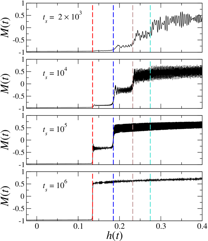
Figure 6: The magnetization in the quantum Ising chain with $L=12$ sites as a function of $h(t)$, for the KZ protocol defined in Eq. (26). Each panel shows data for a different value of $t_{s}$, varying from $2\times 10^{3}$ to $10^{6}$. Vertical dashed lines denote the positions of the avoided crossings between the $|-\rangle$ state and the first four zero-momentum kink-antikink states. The corresponding time scales $T_{k}(L=12)$ are $T_{k}\approx 3.9\times 10^{5}$, $3.6\times 10^{4}$, $1.0\times 10^{4}$, and $4.7\times 10^{3}$, for $k=1,2,3,4$, respectively [see Eq. (45)]. The time scale of the dynamics for $h\approx 0$ is $T(L=12)\approx 4.4\times 10^{9}$, which is much larger than the largest $t_{s}$ considered.

To illustrate the previous scenario, in Fig. 6 we show some results for the magnetization, as obtained for $L=12$ and some values of $t_{s}\ll T(L)\approx 4.4\times 10^{9}$. We observe that, as expected, the magnetization does not change abruptly to a positive value for $h(t)\approx 0$, where it shows a smooth time dependence. The behavior of the data for $h\approx h_{1}(L)$ (red dashed line in Fig. 6), depends on $\Upsilon_{1}=t_{s}/T_{1}(L)$, where $T_{1}(L)=3.9\times 10^{5}$. For $t_{s}=10^{6}>T_{1}(L)$ (bottom panel), the magnetization makes a sudden jump, indicating that the system has essentially moved to the kink-antikink state that makes the avoided level crossing with the negatively magnetized state. Note that magnetization after the jump is approximately 0.5, which should be identified with the magnetization of the kink-antikink state for such a small value of $L$. Equation (13) predicts $M=m_{0}(1-4a_{1}/(3aL^{2/3})$ for $h=h_{1}(L)$. Using $m_{0}\approx 0.96$, $a=1.035$, $a_{1}=2.52$, we obtain $M=0.37$, which is close to the value we observe.

On the other hand, when $t_{s}\ll T_{1}(L)$ (first two top panels) no jump is observed for $h\approx h_{1}(L)$. As discussed below, the transition to a kink-antikink state occurs at one of the following avoided level crossings. Finally, for $t_{s}=10^{5}\sim T_{1}(L)$, corresponding to $\Upsilon_{1}=0.256$, we observe a jump to an intermediate value of $M$, in agreement with the two-level predictions. If one uses $m_{k}\approx 0.5$, Eq. (47) predicts $M\approx-0.38$ as soon as $h(t)$ is larger than $h_{1}(L)$.

VI Multiple avoided level crossings and KZ dynamics

The arguments and results reported in the previous section can be extended to the avoided level crossings occurring for $h=h_{k}(L)$, $k\geq 2$. Each crossing is characterized by a different, yet exponentially large, time scale $T_{k}(L)\sim L/\Delta_{m,k}(L)^{2}$, which decreases with increasing $k$. For a given lattice size $L$ and time scale $t_{s}\ll T(L)$, there is a relevant avoided level crossing $k$ characterized by $t_{s}\ll T_{k-1}(L)$ and $t_{s}\gtrsim T_{k}(L)$. Under these conditions, the system is stuck in the negatively magnetized state $|-\rangle$ for $t<t_{s}h_{k}(L)$. At $h(t)=h_{k}(L)$ the system jumps to a positively magnetized kink-antikink state.

The above scenario is demonstrated by the numerical results of Fig. 7, corresponding to $t_{s}=10^{6}$ and different sizes $L$. For $L=6$ (top panel), the time scale $T(L)$ is one order of magnitude smaller than $t_{s}$ [$T(L=6)\approx 2.4\times 10^{5}$]. As a consequence, the system jumps to the $|+\rangle$ state for $h(t)\approx 0$. For $L=8$, $T(L)=6\times 10^{6}$, which is not much larger than $t_{s}$. Thus, the magnetization of the system is able to make a small jump: For $h\gtrsim 0$ the system goes in a superposition of the $|+\rangle$ state, with a small amplitude, and of the $|-\rangle$ state. At $h(t)\approx h_{1}(L)$, since $t_{s}\gg T_{1}(L)$ [$T_{1}(L=8)\approx 5.3\times 10^{3}$], the $|-\rangle$ state is replaced by the lowest-energy kink-antikink state. For $L=10$ and $12$, no jump occurs at $h=0$, since $t_{s}\ll T(L)$. On the contrary, since $t_{s}\gtrsim T_{1}(L)$ in both cases, we observe a single jump for $h(t)=h_{1}(L)$. The behavior for $L=14$ (bottom) is more complex. Since $t_{s}$ is only slightly smaller than $T_{1}(L)=3.3\times 10^{6}$, we observe a partial jump in the magnetization, indicating that the state is a superposition of the $|-\rangle$ state and of the lowest-energy kink-antikink state for $h\gtrsim h_{1}(L)$. Since $T_{2}(L=14)\approx 2.3\times 10^{5}<t_{s}$, the $|-\rangle$ state disappears at the second avoided level crossing, thus, for $h(t)>h_{2}(L)$, the system is mainly in a superposition of the two lowest-energy kink-antikink states. We observe fast oscillations (with period $T\approx 7$, not visible in the figure) of the magnetization which can be directly related to the energy difference between the two levels [$2\pi/(E_{2}-E_{1})\approx 7.83$], indicating that the matrix element of the magnetization between different kink states is not small. Analogous oscillating behaviors are observed in Fig. 6 for $t_{s}\leq 10^{5}$.

It is interesting to observe that, as $t_{s}$ decreases, the behavior may become more complex, as for $t_{s}=2\times 10^{3}$ in Fig. 6. Indeed, the system may perform several small jumps, becoming eventually a superposition of several kink-antikink states. Moreover, the level spacing of the kink-antikink states decreases as $k$ increases (for $g$ small $E_{k+1}(L)-E_{k}(L)\approx c_{k}L^{-2/3}$ with $c_{k}\sim k^{-1/3}$, see App. A.2) while the gap $\Delta_{k,m}(L)$ increases with $k$. Thus, we may end up in a situation in which the two-level truncation is no longer valid, with several states involved in the crossing. Moreover, as $L$ increases, the kink-antikink levels get closer, so this phenomenon may become more pronounced for large $L$. In the same limit, the different avoided crossings also become closer and closer, since $h_{k+1}(L)-h_{k}(L)\sim L^{-5/3}$, eventually collapsing towards the first crossing $h_{1}(L)\approx a/L$, which might be interpreted as a size-dependent spinodal point.

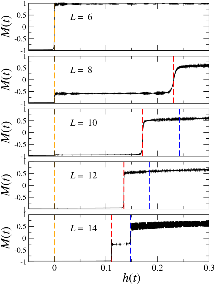
Figure 7: Time-dependence of the magnetization for the KZ protocol, at fixed $t_{s}=10^{6}$ and for different chain sizes ($L=6,\,8,\,10,\,12,\,14$, from top to bottom). The vertical dashed lines indicate the position of the FOQT point $h=0$ (orange) and of the first avoided crossings $h_{k}(L)$, for $k=1$ (red) and $k=2$ (blue). Note that, for the smallest size $L=6$, the dynamics is adiabatic at the FOQT point ($h=0$), where the system exhibits a sudden jump from $|-\rangle$ to $|+\rangle$. In contrast, for $L\gtrsim 8$, the system at $h\approx 0$ remains in the $|-\rangle$ state, until one of the next avoided crossings $h_{k}(L)$ is reached.

We mention that the a similar qualitative behavior for the KZ dynamics in finite-size systems has also been highlighted in Ref. SCD-21 , where it was interpreted as a phenomenon of quantized nucleation. Note, however, that our analysis provides a more thorough description of these out-of-equilibrium phenomena at the FOQTs of quantum Ising models. Indeed, we provide an exact numerical characterization, which is confirmed by an exact perturbative computation, of the size dependence of the values $h_{k}(L)$ of the longitudinal magnetic field where the crossings occur [see Eq. (17)]. In particular, this implies their collapse onto a single (spinodal) point in the limit in which the magnetic energy $hL$ is kept fixed as $L\to\infty$. Finally, we provide a general EFSS theory for the avoided crossings, which allows us to provide a quantitative estimate of the time scales $T_{k}(L)$. These results are crucial to quantitatively interpret how the observed behavior depends on $t_{s}$.

VII The KZ protocol in the thermodynamic limit

We finally turn to the investigation of the out-of-equilibrium behavior arising in the KZ evolution in the thermodynamic limit. The analysis presented in the previous sections is only valid in the finite-size limit, in which $hL$ is fixed and not too large. On the other hand, if we consider the behavior for $L\to\infty$ and fixed magnetic field, the avoided level crossings collapse towards $h=0$. Therefore, if a scaling behavior occurs in this limit, it may not be described by a straightforward extension of the OFSS results.

In the absence of a theoretical framework, we investigate the KZ dynamics in the infinite-size limit numerically. Unfortunately, even after exploiting momentum conservation, the numerics based on exact diagonalization is limited to relatively small system sizes, up to a few tens of sites. Nevertheless, as we shall see, an appropriate analysis of the finite-size data allows us to unveil a scaling picture of the behavior of the KZ dynamics in the thermodynamic limit.

To study the infinite-size limit at fixed $h$, we follow the following two-step procedure: (i) we first determine the large-$L$ limit at fixed time scale $t_{s}$, by sequentially increasing $L$ until the relevant observables $O(t,t_{s},L)$ approach essentially $L$-independent quantities $O_{\infty}(t,t_{s})$, as a function of $h(t)=t/t_{s}$; (ii) we study the behavior of the infinite-size limits $O_{\infty}(t,t_{s})$ as a function of $t_{s}$, looking for a scaling behavior in terms of the variables $t$ and $t_{s}$, for large values of $t_{s}$.

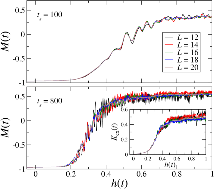
Figure 8: Evolution of the magnetization $M(t)$ in the KZ protocol, for $t_{s}=100$ (top) and $t_{s}=800$ (bottom), and for various values of $L$ (see legend). Data are plotted versus $h(t)=t/t_{s}$. The inset in the bottom panel shows the time behavior of the excess energy $K_{\rm ex}(t)$ defined in Eq. (31). In all cases the data appear to approach a well defined large-$L$ limit.

The procedure corresponding to step (i) is exemplified in Fig. 8, which displays the time evolution of the longitudinal magnetization $M(t)$ defined in Eq. (29) for $t_{s}=100$ (top) and $t_{s}=800$ (bottom), and various values of $L$. For $t_{s}=800$, we also report data for the excess energy $K_{\rm ex}(t)$ defined in Eq. (31). We observe that the different data sets apparently converge to an asymptotic large-$L$ behavior, which provides the time dependence of the infinite-size magnetization $M_{\infty}(t,t_{s})$ and of the excess energy $K_{{\rm ex},\infty}(t,t_{s})$ at the given value of $t_{s}$. Convergence is faster for small time scales, as is visible from the top panel. In contrast, when $t_{s}$ increases, fast oscillations in time emerge, although their amplitude decreases with $L$ and a qualitative asymptotic behavior can be recognized already for moderate chain lengths $L\approx 20$ (bottom panel). The behavior of the excess energy $E_{\rm ex}(t)$ defined in Eq. (30) (not shown) resembles that of $K_{\rm ex}(t)$, although with wider time oscillations, which are induced by the transverse-field energy contribution.

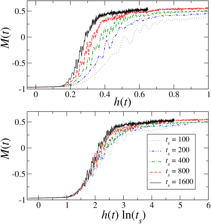
Figure 9: The infinite-size magnetization for different KZ protocols, plotted versus $h(t)=t/t_{s}$ (top panel) and versus $\Omega\equiv h(t)\ln t_{s}$ (bottom panel). The dynamics starts from $h_{i}=-0.05$ in all cases. Data are for a system of size $L=20$, ensuring that the large-$L$ limit is approached for all the considered values of $t_{s}$. Note that the curves tend to collapse on a single curve for sufficiently large values of $t_{s}$, when they are plotted versus $\Omega$ (bottom panel). This suggests the existence of a nontrivial large-$t_{s}$ scaling limit in terms of $\Omega$.

In step (ii) we compare the infinite-size time evolutions of the observables for several increasing time scales $t_{s}$, looking for the emergence of a scaling behavior. The top panels of Figs. 9 and 10 show some results for the longitudinal magnetization $M(t)$ and for the excess energy $K_{\rm ex}(t)$ versus $h(t)$, respectively. The different curves correspond to $t_{s}$ varying from $100$ to $1600$; for these values of $t_{s}$, we have a sufficiently good numerical evidence that the time evolutions obtained for $L=20$ (see Fig. 8) can be effectively considered as infinite-size behaviors. We note that the magnetization changes sign for values of $h$ that decrease with increasing $t_{s}$, suggesting that the sign change occurs for values of $h$ that approach $h(t)=0$ (thus $t=0$) as $t_{s}\to\infty$.

The plots reported in the lower panels of Figs. 9 and 10 show an apparent collapse of the infinite-size magnetization and excess-energy curves when plotted versus

$$\Omega(t)=h(t)\,\ln t_{s}={t\ln t_{s}\over t_{s}}.$$ (49)

Therefore, they suggest a peculiar infinite-size scaling behavior for large values of $t_{s}$, that is

$$M_{\infty}(t,t_{s}) \approx m_{0}\,{\cal M}_{\infty}(\Omega),$$ (50)

$$K_{{\rm ex},\infty}(t,t_{s}) \approx {\cal K}_{{\rm ex},\infty}(\Omega).$$ (51)

Notice that $\Omega$ definitely differs from the naive large-size scaling variable $W$ that is derived in the OFSS framework, cf. Eq. (42). Equation (50) predicts that the longitudinal magnetization changes sign for a fixed value of $\Omega$ and therefore for $h(t)\sim 1/\ln t_{s}$, somehow resembling a spinodal-like behavior. Further studies are required to make this scenario more solid.

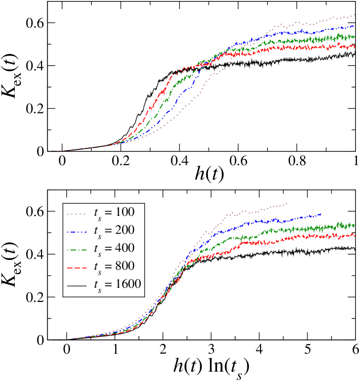
Figure 10: The excess energy $K_{\rm ex}$, as defined in Eq. (31), for the same KZ evolutions reported in Fig. 9. Data are for $L=20$, ensuring that the large-$L$ limit is obtained. As for the magnetization, we observe an apparent data collapse, when they are plotted versus $\Omega$. The data show a slower approach to the scaling curve in the large-$\Omega$ region, $\Omega\gtrsim 4$, where the magnetization is almost constant and independent of $t_{s}$ ($M\approx 0.5$, for these values of $\Omega$, see Fig. 9).

We conclude by noting that the magnetization, displayed in Fig. 9, is almost constant (apart from short-time fluctuations), $M_{\infty}(t\to\infty,t_{s})\approx 0.5$, for sufficiently large values of $\Omega$. The significant deviation from 1, which is the ground-state value for $h\to\infty$, can be explained by the large energy excess, therefore by the fact that the KZ protocol has injected a relatively large amount of energy (work to change $h$) in the system, giving rise to a significant departure from the ground state of the Hamiltonian at large times. This is clearly evident in the behavior of the excess energy $E_{\rm ex}$ (not shown), which is qualitatively analogous to the curves of $K_{\rm ex}$ reported in Fig. 10.

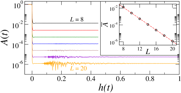
Figure 11: The adiabaticity function $A(t)$ for KZ protocols starting from $h_{i}=-0.05$ and with a time scale $t_{s}=800$. Results for different system sizes $L=8,\,10,\,12,\,14,\,16,\,18,\,20$ (top to bottom curves). The inset shows the value $\bar{A}$ obtained by averaging the numerical data for $h(t)\in[0.5,1]$; the straight line is an exponential fit $\bar{A}=A_{0}\exp(-\alpha L)$, with $\alpha\approx 0.772$.

To gain further insight on the features of such stationary states, in Fig. 11 we focus on the adiabaticity function defined in Eq. (32). For $h\approx 0$, we observe a sudden drop of $A(t)$ to a stationary value $\bar{A}$ close to zero, meaning that, as soon as the FOQT point is crossed, the state of the system becomes nearly orthogonal to the instantaneous ground state at the corresponding field $h(t)$. As discussed in the previous Sections, this happens as soon as the KZ time scale $t_{s}$ is much smaller than $T(L)$, the characteristic time associated with the avoided level crossing at $h=0$. Indeed, $T(L)$ varies from $T(L\!=\!8)\approx 7.28\times 10^{6}$ to $T(L\!=\!20)\approx 8.36\times 10^{14}$, and is in all cases much larger than $t_{s}=800$, the value used in the KZ dynamics considered in the figure. We remark that the asymptotic stationary value $\bar{A}$ is almost insensitive to the choice of the time scale $t_{s}\ll T(L)$, while it decreases exponentially with the system size $L$, as reported in the inset. In particular, a numerical fit of our data obtained with $t_{s}=800$ gives $\bar{A}(L)\sim e^{-\alpha L}$, with $\alpha\approx 0.772$.

Finally, in Fig. 12 we show the connected part of the correlation function of the longitudinal magnetization, for a system with $L=20$ spins. Assuming translational invariance, it is defined as

$$C_{c}(r,t)=\langle\Psi(t)|\sigma^{(1)}_{x}\sigma^{(1)}_{x+r}|\Psi(t)\rangle-\langle\Psi(t)|\sigma^{(1)}_{x}|\Psi(t)\rangle^{2}.$$ (52)

Our data are plagued by oscillations in time, whose frequency increases with $t_{s}$. Such oscillations diminish for larger system sizes, which, unfortunately, we were only able to increase up to $L\approx 20$. Nonetheless we observe that, apart from the intermediate-time transient region around $h(t)\approx 0.3$, corresponding to the time at which the magnetization changes sign (compare with the dashed red curve for $t_{s}=800$ in the top panel of Fig. 9), the system is always weakly spatially correlated and the correlation length is of the order of one.

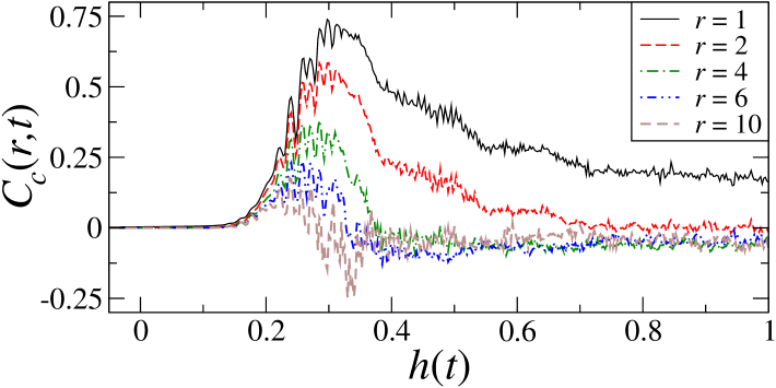
Figure 12: Connected correlation function of the longitudinal magnetization $C_{c}(r,t)$, evaluated at various distances $r\leq L/2$, for a chain of length $L=20$. Results are for the same KZ evolutions considered in Fig. 11.

VIII Summary and conclusions

We have addressed the out-of-equilibrium dynamics of quantum Ising models in a transverse field, driven across their FOQTs by a homogeneous longitudinal external field $h$. Specifically, we focus on the quantum spin chain with Hamiltonian (1) and periodic boundary conditions, which provides a paradigmatic model for which we can obtain accurate numerical results that can be used to verify our theoretical predictions. We consider a dynamic KZ protocol in which the longitudinal field $h$ is varied linearly in time, with a time scale $t_{s}$, i.e, $h(t)=t/t_{s}$, across the FOQT at $h=0$. The system starts from the negatively magnetized ground state at $h_{i}\equiv h(t_{i})<0$, and then it evolves unitarily according to the Schrödinger equation for $t>t_{i}$, up to positive values of $h(t)$, eventually leading to states with positive longitudinal magnetization. We analyze the time evolution of some relevant observables, such as the longitudinal magnetization and the excess energy, identifying scaling regimes involving the system size $L$ and the time scale $t_{s}$ of the KZ protocol. We also discuss the behavior in the infinite-size limit, keeping $t_{s}$ fixed.

In finite-size systems, we identify an OFSS regime whenever the system is close to one of the avoided level crossings that characterize the spectrum in the presence of the longitudinal field $h$. In particular, at the FOQTs for $g<1$, since periodic boundary conditions preserve the ${\mathbb{Z}}_{2}$ symmetry of the model, an avoided level crossing occurs for $h=0$, where the actual eigenstates are superposition of the positively and negatively magnetized states, with an energy gap $\Delta(L)$ that decays exponentially with $L$, i.e., $\Delta(L)\sim e^{-bL}$ with $b\approx-\ln g$. The quantum evolution of finite-size systems driven across $h=0$ shows an OFSS behavior PV-24 ; RV-21 ; PRV-18-def ; PRV-20 , when $L\to\infty$ and $t_{s}\to\infty$ simultaneously, keeping appropriate combinations of $L,t_{s},t$ fixed. A crucial scaling variable is the time-scale ratio $\Upsilon=t_{s}/T(L)$, where $T(L)\sim L\Delta(L)^{-2}$ is the time scale associated with the passage across the avoided level crossing. In particular, if $t_{s}\gg T(L)$ the system evolves adiabatically, thus switching from the negatively magnetized state to the positively magnetized one as it crosses $h=0$. On the other hand, if $t_{s}\ll T(L)$, the passage across $h=0$ is effectively instantaneous, so that the system persists in the wrongly magnetized state ($M<0$) for $h(t)>0$.

Besides the avoided crossing at $h=0$, the spectrum of finite-size systems shows a sequence of avoided level crossings between the ${\rm wrongly}$ magnetized state and a discrete series of zero-momentum kink-antikink states, labeled by $k=1,2,\ldots$. These avoided crossings are localized at $h_{k}(L)=a/L+a_{1k}/L^{5/3}+O(L^{-2})$, where the leading term does not depend on $k$, so that they get closer and closer with increasing $L$, as $h_{k}-h_{k^{\prime}}\sim L^{-5/3}$. The minimum energy differences $\Delta_{m,k}$ at each avoided crossing are exponentially small with increasing $L$, i.e., $\Delta_{m,k}\sim e^{-b_{k}L}$. Moreover, $\Delta_{m,k}(L)$ increases with $k$, $\Delta_{m,k}(L)<\Delta_{m,k+1}(L)$, and is always larger than $\Delta(L)$. These predictions have been verified numerically for $k$ up to 5 on systems of size up to $L=26$. We conjecture that these features also hold for higher excited states, for sufficiently low energies, smaller than the values where qualitatively different states appear (for example, we must require at least $k/L\lesssim 1/2$).

The dynamic behavior across these additional avoided crossings is analogous to that discussed for the avoided level crossing at $h=0$. They also admit an OFSS description in terms of the analogous scaling variable $\Upsilon_{k}=t_{s}/T_{k}(L)$, where $T_{k}(L)\sim L\Delta_{m,k}(L)^{-2}$. Such OFSS behavior can be observed because it occurs in a very small range of values of $h$ around $h_{k}(L)$, i.e., for $|h-h_{k}(L)|\sim\Delta_{m,k}(L)/L$, much smaller than the $O(L^{-5/3})$ spacing between subsequent level crossings. Note that $T(L)\gg T_{1}(L)\gg T_{2}(L)\gg\ldots$ since $\Delta(L)\ll\Delta_{m,1}(L)\ll\Delta_{m,2}(L)\ldots$.

The previous results allow us to predict the behavior of the system along the KZ evolution. According to the OFSS theory, if the system starts in the ground state for $h<0$, i.e., in the negatively magnetized state, it may jump to a state with positive magnetization at $h_{k}(L)$ only if $t_{s}\gtrsim T_{k}(L)$. Since the time scales satisfy $T(L)\gg T_{1}(L)\gg T_{2}(L)\gg\ldots$, the time scale $t_{s}$ of the KZ protocol can be tuned in such a way to select at which avoided crossing the system magnetization changes sign. More precisely, when $t_{s}$ is large but still satisfies $t_{s}\ll T(L)$, the negatively magnetized state effectively survives across the $h=0$ and the first $k-1$ avoided level crossings up to the one satisfying $t_{s}\approx T_{k}(L)$. When $h(t)\approx h_{k}(L)$, then the system jumps to a kink-antikink state with positive magnetization. We have shown that this scenario is actually realized, by reporting numerical results for the quantum evolution of systems along KZ protocols up to $L=20$ and $t_{s}=10^{6}$.

As already stressed, the avoided level crossings related to kink-antikink bound states collapse to $h=0^{+}$ in the infinite-size limit. This makes the study of the thermodynamic limit (defined as the limit $L\to\infty$ keeping $t$ and $t_{s}$, and therefore $h(t)$, constant) problematic. We study such limit numerically, by first determining the large-volume behavior at fixed $t_{s}$, and then analyzing the behavior with increasing $t_{s}$, looking for the scaling behavior that characterizes the out-of-equilibrium behavior of the infinite-size systems across the FOQT. Our analysis shows that the negatively magnetized state jumps to states with positive magnetization at values $h_{\star}(t_{s})>0$ that approach $h=0$ with increasing $t_{s}$. On the basis of the numerical results, we conjecture that $h_{\star}(t_{s})\sim 1/\ln t_{s}$, which suggests an infinite-size scaling behavior in terms of the scaling variable $\Omega=t\ln t_{s}/t_{s}$. Another notable feature of the dynamics is that the quantum Ising system approaches a nontrivial stationary state in the large-$t$ limit, characterized by an energy significantly larger than that of the corresponding magnetized ground state. This large energy difference is clearly related to the average work done when varying $h$ in the KZ protocol. It is important to stress that this infinite-size behavior is not obtained by a straightforward extension of the finite-size analyses based on the OFSS behaviors across the avoided level crossings. Of course, additional computations are called for to conclusively support the above infinite-volume scenario. In particular, to improve the evidence of the scaling behavior, results for larger sizes would be highly desirable.

We finally remark that the spinodal-like behavior observed here shows notable similarities with that observed when short-range classical systems are driven across a first-order transition by varying a Hamiltonian parameter with time, even if the dynamics is different: results with a purely relaxational dynamics are reported, e.g., in Refs. PV-17 ; PV-25 .

Although the above results have been obtained for quantum Ising chains with periodic boundary conditions, we believe that several features have general validity. For example, apart from specific details, the general scenario for finite-size and infinite-size systems should apply to open and parallel fixed boundary conditions. This is desirable from a numerical point of view, since one could employ methods, such as the density-matrix renormalization group, which are best suited to simulate chains with open ends and which would enable us to obtain results for larger system sizes, potentially up to $L\gtrsim 100$. Some differences are expected when considering antiperiodic and opposite fixed boundary conditions, since the lowest-energy states are kink states CNPV-14 ; PRV-18-fowb ; PRV-20 , separating regions with different magnetization. It would be tempting to understand how the infinite-volume out-of-equilibrium behavior is realized there. We believe that a similar scaling behavior should also emerge in higher dimensions, such as in the two- and three-dimensional quantum Ising models. Another interesting issue is related to the role of dissipation, which can be introduced by using, e.g., the Lindblad framework RV-21 ; DRV-20 .

We point out that the out-of-equilibrium scaling behaviors reported in this paper have been numerically observed in relatively small systems. Therefore, given the need for high accuracy without necessarily reaching scalability to large sizes, it would be tempting to employ the available technology to check these predictions experimentally, using, for instance, ultracold atoms in optical lattices Bloch-08 ; Simon-etal-11 , trapped ions Edwards-etal-10 ; Islam-etal-11 ; LMD-11 ; Kim-etal-11 ; Richerme-etal-14 ; Jurcevic-etal-14 ; Debnath-etal-16 , as well as Rydberg atoms in arrays of optical microtraps Labuhn-etal-16 ; Guardado-etal-18 ; Keesling-etal-19 ; BL-20 or even quantum computing architectures based on superconducting qubits Barends-etal-16 ; Gong-etal-16 ; CerveraLierta-18 ; Ali-etal-24 . Some recent experiments have already addressed the dynamics and the excitation spectrum of quantum Ising-like chains Gong-etal-16 ; LTDR-24 ; DMEFY-24 , thus opening possible avenues where the envisioned behaviors at FOQTs can be observed in the near future.

Appendix A Kink-antikink states: scaling analysis of the energies and magnetizations

In this Appendix we compute the energy and the magnetization of the kink-antikink states for a chain of $L$ spins, to first order in the transverse magnetic field $g$. We mainly consider periodic boundary conditions, but we will also address systems with fixed parallel boundary fields. We will obtain exact results for the energies of kink-antikink states for finite values of $L$, generalizing the results of Refs. MW-78 ; Rutkevich-08 ; Coldea-etal-10 ; Rutkevich-10 . We then obtain scaling results for small values of $h$ and large values of $L$, more precisely, for $g$ small and in the finite-size scaling regime in which $h\to 0$ and $L\to\infty$ simultaneously, keeping the magnetic energy $hL$ fixed. Phenomenologically, the scaling regime occurs when $h/g$ is small, but still satisfies the condition $h/g\gg L^{-3}$. Note that the perturbative approach also requires the magnetic energy $hL$ to be small with respect to the spacing $4J$ of the levels for $g=h=0$, thus our results hold only for $h\ll 4/L$ (we recall that $J=1$).

A.1 Secular equation

The spectrum of the model has been discussed in Sec. II.2. For $g=h=0$ the kink-antikink states are degenerate with energy $E_{k}=4J+E_{gs}$, where $E_{gs}$ is the energy of the fully magnetized lowest-energy degenerate states. To determine the energy for $g\not=0$, we note that, because of the periodic boundary conditions, the Hamiltonian is translation invariant. This implies that the Hamiltonian restricted to the subspace spanned by the kink-antikink states is the sum of $L$ blocks, each of them of size $L-1$. Each block is specified by a momentum $p=2\pi k/L$, with $k=0,\ldots,L-1$, with basis (we write it explicitly for $L=4$):

$$|p,1\rangle = \tfrac{1}{2}\left(|-1,1,1,1\rangle+e^{ip}|1,-1,1,1\rangle+\right.$$

$$\quad\left.e^{2ip}\ |1,1,-1,1\rangle+e^{3ip}\ |1,1,1,-1\rangle\right),$$

$$|p,2\rangle = \tfrac{1}{2}\left(|-1,-1,1,1\rangle+e^{ip}\ |1,-1,-1,1\rangle+\right.$$

$$\quad\left.e^{2ip}\ |1,1,-1,-1\rangle+e^{3ip}\ |-1,1,1,-1\rangle\right),$$

$$|p,3\rangle = \tfrac{1}{2}\left(|-1,-1,-1,1\rangle+e^{ip}\ |1,-1,-1,-1\rangle+\right.$$

$$\quad\left.e^{2ip}\ |-1,1,-1,-1\rangle+e^{3ip}\ |-1,-1,1,-1\rangle\right).$$

The Hamiltonian restricted to each block takes a tridiagonal form. The only nonvanishing elements are

$$H_{n,n} = 4J+E_{\rm gs}+2hn-hL,$$

$$H_{n,m} = g(1+e^{ip}),\qquad\,\,\,\,n-m=1,$$

$$H_{n,m} = g(1+e^{-ip}),\qquad n-m=-1,$$ (54)

where $1\leq n,m\leq L-1$. Note that the Hermitian conjugate of $H(p)$ is $H(2\pi-p)$, so, for $p\not=0,\pi$, the spectrum is doubly degenerate, a result which is not specific of the perturbative analysis, but holds in general.

To determine the spectrum of $H$, we compute

$$D(\ell,{E})=\det(H-{E}I)\,,$$ (55)

where $I$ is the identity matrix and $\ell=L-1$ is the dimension of the matrix associated with $H$. To simplify the notation, we define

$$b={1\over 2h}(4J+E_{gs}+hL),\quad z={2g\over h}\cos(p/2),\quad f=2h,$$ (56)

so that $H-{E}I$ takes the form (again we write it explicitly for $L=4$)

$$\begin{pmatrix}f(b-3)-{E}&{1\over 2}fze^{-ip/2}&0\\[5.69054pt] {1\over 2}fze^{ip/2}&f(b-2)-{E}&{1\over 2}fze^{-ip/2}\\[5.69054pt] 0&{1\over 2}fze^{ip/2}&f(b-1)-{E}\end{pmatrix}\,.$$ (57)

For $h=0$, the determinant and the spectrum of $H$ is easily determined (see, e.g., App. B.2 of Ref. CPV-15-iswb ). The energies of the $n$ levels are:

$$E_{n}=E_{gs}+4J-4g\cos{p\over 2}\cos{\pi n\over L}.$$ (58)

Here we will use the same methods to obtain an exact result for $h\not=0$.

By using the properties of the determinant (we expand with respect to the last row), we obtain the recursion relation:

$$D(\ell,E) = [f(b-1)-{E}]D(\ell-1,{E}+f)$$ (59)

$$-{f^{2}z^{2}\over 4}D(\ell-2,{E}+2f)\,,$$

which holds for any $\ell\geq 2$, provided we set $D(1,{E})=f(b-1)-{E}$ and $D(0,{E})=1$. To solve it, we fix $\ell$ and define

$$a_{k}=\left({fz\over 2}\right)^{-k}D[k,{E}+(L-1-k)f].$$ (60)

By replacing $\ell$ with $k+1$ and ${E}$ with ${E}-(k+2-L)f$, we obtain

$$a_{k+1}={2\over z}(k+c)a_{k}-a_{k-1},\quad c=b-L+1-{E}/f.$$ (61)

The solution of the recursion can be obtained by noting that the Bessel function of the first kind $J_{\nu}(z)$ and the Neumann-Weber function (Bessel function of the second kind) $N_{\nu}(z)$ satisfy a similar recursion relation. Using Eq. (8.417) of Ref. GradRi with $\nu=k+c$ we find

$$Z_{k+c+1}(z)={2\over z}(k+c)Z_{k+c}(z)-Z_{k+c-1}(z)$$ (62)

with $Z=J$ or $Z=N$. Thus, we can write the general solution as

$$a_{k}=AJ_{k+c}(z)+BN_{k+c}(z).$$ (63)

The coefficients $A$ and $B$ are fixed by the condition that $a_{0}=1$ and $a_{1}=2c/z$. We obtain

$$A = -{1\over C}\left[2cN_{c}(z)-zN_{1+c}(z)\right],$$

$$B = {1\over C}\left[2cJ_{c}(z)-zJ_{1+c}(z)\right],$$

$$C = z\left[J_{c}(z)N_{1+c}(z)-J_{1+c}(z)N_{c}(z)\right].$$ (64)

Using Eq. (8.477) of Ref. GradRi , $C=-2/\pi$. Moreover, from Eq. (62) with $k=0$, we finally obtain

$$A={\pi z\over 2}N_{-1+c}(z),\quad B=-{\pi z\over 2}J_{-1+c}(z).$$ (65)

We have thus an exact expression for $a_{k}$. Setting $k=\ell=L-1$ we obtain an exact result for the determinant:

$$D(\ell,{E})={\pi z\over 2}\left({fz\over 2}\right)^{L-1}\times$$ (66)

$$\quad\times\Bigl{[}N_{-1+c}(z)J_{L-1+c}(z)-J_{-1+c}(z)N_{L-1+c}(z)\Bigr{]},$$

which depends on the energy $E$ only through the variable $c$ defined in Eq. (61).

A.2 Spectrum

Using Eq. (66) we can obtain the spectrum of $H$. Indeed, for given $p,h$, and $L$, we can first compute $z$ and then determine the solutions $\nu_{n}(z)$ of the equation

$$N_{\nu}(z)J_{\nu+L}(z)-J_{\nu}(z)N_{\nu+L}(z)=0,$$ (67)

where we set $\nu=c-1$. The energies are given by

$${E}_{n}=E_{gs}+4J-hL-2h\nu_{n}(z).$$ (68)

We now wish to determine the behavior of ${E}_{n}$ for $L\to\infty$, $h\to 0$, keeping the ratio $hL$ fixed. We assume $h$ positive, so that $z\to+\infty$ in the $h\to 0$ limit. As for $\nu$, we have numerically verified that the solutions of the secular equation (67), also diverge ($\nu_{n}(z)\to+\infty$) but the ratio $\nu_{n}(z)/z$ converges to a constant in the limit. Under these conditions, a systematic use of the expansion (8.452) of Ref. GradRi allows us to prove that the ratio

$${N_{\nu}(z)\,J_{\nu+L}(z)\over J_{\nu}(z)\,N_{\nu+L}(z)}$$ (69)

vanishes exponentially in the infinite-length limit. Thus, with exponential precision we obtain that the quantities $\nu_{n}(z)$ satisfy the equation

$$J_{\nu}(z)=0.$$ (70)

Asymptotic results for the Bessel function in the limit of large $\nu$ and $z$ are reported in Refs. Olver-54a ; Olver-54b ; JL-12 . In particular, an asymptotic formula for the zeroes is reported in Ref. Olver-54b , see Eq. (7.1). To leading order, they can be obtained by solving

$$\mathop{\rm Ai}(\nu^{2/3}\zeta)=0,$$ (71)

where $\mathop{\rm Ai}(z)$ is the Airy function and $\zeta$ is a function of $y=z/\nu$. The zeroes of the Airy function all belong to the negative real axis Olver-54b , and this requires the function $\zeta$ to be negative which only occurs for $y>1$. In this interval of values of $y$, $\zeta$ is given by

$$\zeta(y)=-\left({3\over 2}\right)^{2/3}\left[\sqrt{y^{2}-1}-\arccos(1/y)\right]^{2/3}.$$ (72)

Note that $\zeta(y)$ goes to zero for $y\to 1$ as

$$\zeta(y)\approx-2^{1/3}(y-1)\left[1-{3\over 10}(y-1)\right].$$ (73)

Thus, if $\alpha_{n}$ are the zeroes of the Airy function ($\alpha_{n}<0$), we have

$$\nu_{n}(z)\approx\nu_{{\rm e},n}=z\,(1-|\alpha_{n}|2^{-1/3}z^{-2/3}).$$ (74)

The approximation becomes exact for $z\to\infty$, since

$$J_{\nu_{{\rm e},n}}(z)\sim z^{-1}.$$ (75)

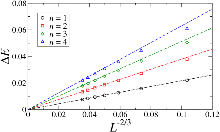
Figure 13: Plot of $\Delta E={E}-E_{gs}-4J+hL+4g$, for $hL=1/10$, $g=1/100$, $p=0$, and values of $L$ ranging from 30 to 150. We report the four lowest energies. The straight lines are obtained by using the approximate formula (77).

Collecting all these results and using the explicit expression for $z$, Eq. (56), we end up with

$${E}_{n} \approx E_{gs}+4J-hL$$

$$-4g\cos(p/2)\left[1-{|\alpha_{n}|\over 2}\left({h\over g\cos(p/2)}\right)^{2/3}\right].$$

Note that the nonanalytic term is of order $L^{-2/3}$ at fixed $hL$. Corrections are of order $1/L$. Finally, note that $p$ vanishes as $1/L$. Thus, to order $L^{-2/3}$, there is no $p$ dependence: We expect the degeneracy in $p$ to be lifted only at order $1/L^{2}$, as in the absence of magnetic field. We thus obtain

$${E}_{n}=E_{gs}+4J-hL-4g\left[1-{|\alpha_{n}|\over 2}\left({h\over g}\right)^{2/3}\right]+O(L^{-1}).$$ (77)

It is important to stress that this result only holds in the limit $h\to 0$, $L\to\infty$ at fixed $hL$. More precisely, it does not hold for $h\to 0$ at fixed $L$, since for finite sizes the behavior is analytic in $h$. In this limit, the magnetic-field corrections are of order $h^{2}$ at fixed $L$, because of the symmetry under $h\to-h$. This analytic behavior should be observed when the magnetic energy, of order $hL$, is much smaller than the splitting of the levels due to the transverse field, which is of the order of $g/L^{2}$ [more precisely, $E_{n}-E_{1}\approx 2\pi^{2}g(n^{2}-1)/L^{2}$, see Eq. (58)], i.e., for $h\ll gL^{-3}$. Equation (77) applies instead for $h\gg gL^{-3}$. Indeed, if this condition holds, the magnetic energy $hL$ is much larger than the correction term of order $g^{1/3}h^{2/3}$.

The expansion depends on the zeroes of the Airy function. The smallest zeroes correspond to $\alpha_{n}=-2.33811,\,-4.08795,\,-5.52056,\,-6.78671,\,-7.94413$ for $n=1,2,3,4,5$. For larger values of $n$, we can use the asymptotic formula

$$\alpha_{n}\approx-\left[{3\pi\over 8}(4n-1)\right]^{2/3}.$$ (78)

This is a reasonable approximation even for $n=1$, as it predicts $\alpha_{1}\approx-2.32$, which should be compared with the exact result $\alpha_{1}=-2.33811\ldots$. For the spacing of the levels we thus predict

$$E_{n+1}-E_{n}\approx c_{n}\left({h\over g}\right)^{2/3},$$ (79)

where $c_{n}$ decreases with $n$ ($c_{n}\sim n^{-1/3}$ for $n$ not too small).

A.3 Magnetization

We now focus on the behavior of the magnetization $M$, defined as

$$M={1\over L}\langle\Psi|\sum_{x}\sigma_{x}^{(1)}|\Psi\rangle,$$ (80)

where $|\Psi\rangle$ is a generic normalized state. To determine its scaling behavior, we define a density function $\rho(m)$. If

$$|\Psi\rangle=\sum_{i}B_{i}|\Psi_{i}\rangle,$$ (81)

where $|\Psi_{i}\rangle$ is an eigenstate of the magnetization operator with eigenvalue $m_{i}$, $\rho(m)$ is defined so that

$$\int_{a}^{b}dm\,\rho(m)=\sum_{i:a\leq m_{i}\leq b}|B_{i}|^{2},$$ (82)

for any $-1\leq a\leq b\leq 1$. The density $\rho(m)$ satisfies

$$\int_{-1}^{1}dm\,\rho(m)=1,\qquad\int_{-1}^{1}dm\,m\rho(m)=M.$$ (83)

We have determined $\rho(m)$ for the lowest eigenstates of the kink-antikink Hamiltonian, finding that $\rho(m)$ is strongly peaked around $m\approx 1$, with a width that goes to zero as $L\to\infty$. More precisely, it satisfies the scaling law (see Fig. 14)

$$\rho(m)\approx L^{2/3}F(X),\qquad X=(1-m)L^{2/3},$$ (84)

which in turn implies

$$M\approx 1-L^{-2/3}\int dX\,XF(X),$$ (85)

We thus conclude that, in the infinite-size limit, the kink-antikink states are fully magnetized as the ground state, with corrections of order $L^{-2/3}$.

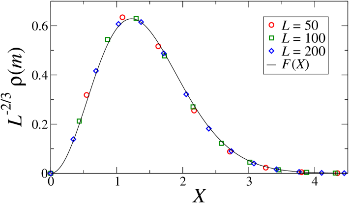
Figure 14: Plot of $L^{-2/3}\rho(m)$ versus $X=(1-m)L^{2/3}$, for $hL=1/10$, $g=1/100$, $p=0$ and three values of $L$. We consider the lowest-energy ($n=1$) kink-antikink state. We also report the scaling furve $F_{n}(X)$ computed using Eq. (94).

To verify Eq. (84) and compute the scaling function $F(X)$, let us expand the eigenstates of the kink-antikink Hamiltonian in terms of the vectors $|p,i\rangle$ defined in Eq. (A.1), which are eigenstates of the magnetization operator with eigenvalue $m_{i}=1-2i/L$:

$$|\Psi\rangle=\sum_{i}B_{i}\,|p,i\rangle.$$ (86)

The coefficients $B_{i}$ satisfy the recursion relation

$$e^{ip/2}B_{k-1}+{2\over z}(k+c-1)B_{k}+e^{-ip/2}B_{k+1}=0,$$ (87)

$k=1,\ldots,L-1$, with boundary conditions $B_{0}=B_{L}=0$. This is the analogue of Eq. (61). The general solution is

$$B_{k}=d(-1)^{k}e^{ipk/2}\left[N_{\nu}(z)J_{k+\nu}(z)-J_{\nu}(z)N_{k+\nu}(z)\right],$$ (88)

satisfying the condition $B_{L}=0$, because of Eq. (67). Here $d$ is a function of the system parameters that is fixed by the normalization condition $\langle\Psi|\Psi\rangle=1$. As before, we have defined $\nu=c-1$.

The previous result is exact for any value of $L$. For large sizes, we can use the fact that the secular equation can be simply written as $J_{\nu}(z)=0$. Therefore, we obtain

$$B_{k}=d^{\prime}(-1)^{k}e^{ipk/2}J_{k+\nu}(z),$$ (89)

with $d^{\prime}=dN_{\nu}(z)$. Note that the momentum $p$ appears only as a phase, and thus the results for the magnetization depend on $p$ only through the variable $z$. The function $\rho(m)$ can be estimated by setting

$$\rho(m)={L\over 2}|B_{k}|^{2}\qquad\hbox{for}\;\;{(2k-1)\over L}\leq 1-m\leq{(2k+1)\over L}.$$ (90)

The scaling function $F(X)$ is then defined as

$$F(X)=\tfrac{1}{2}L^{1/3}|B_{XL^{1/3}/2}|^{2}.$$ (91)

To evaluate the scaling function, we need the asymptotic expansion of $J_{k+\nu}(z)$ for $z\to\infty$ and $\nu=\nu_{n}(z)$. Using the results of Refs. Olver-54a ; Olver-54b ; JL-12 , in the scaling limit we obtain the asymptotic expansion

$$J_{k+\nu}(z)=2^{1/3}z^{-1/3}\mathop{\rm Ai}(\xi_{n}(X))[1+O(z^{-2/3})],$$ (92)

where

$$\xi_{n}(X) = \alpha_{n}+2^{1/3}z^{-1/3}k$$ (93)

$$= \alpha_{n}+\left[{hL\over g\cos(p/2)}\right]^{1/3}{X\over 2}.$$

As before, since $p\sim 1/L$, only subleading corrections depend on $p$, so we can set $p=0$. The scaling function for the $n^{\rm th}$ kink-antikink state is given by

$$F_{n}(X)={1\over 2N_{1,n}}\left({hL\over g}\right)^{1/3}\mathop{\rm Ai}[\xi_{n}(X)]^{2},$$ (94)

where the prefactor has been determined by requiring $F(X)$ to be normalized. The constant $N_{1,n}$ is given by

$$N_{1,n}=\int_{\alpha_{n}}^{\infty}dx\,\mathop{\rm Ai}(x)^{2};$$ (95)

for $n=1$, we have $N_{1,1}\approx 0.491697$. The scaling result (94) is reported in Fig. 14: the agreement with the numerical data is excellent.

To check the previous results, we compare the magnetization computed using Eq. (94) with the expression that follows from the Hellmann-Feynman theorem:

$${M}_{n} = -{1\over L}{\partial{E}_{n}\over\partial h}$$ (96)

$$= 1-{4|\alpha_{n}|\over 3}\left({g\over hL}\right)^{1/3}L^{-2/3}.$$

If we use Eq. (94), we obtain the same scaling behavior. The constant $4|\alpha_{n}|/3$ is replaced by $N_{2,n}$ where

$$N_{2,n}={2\over N_{1,n}}\int_{\alpha_{n}}^{\infty}dx\,(x-\alpha_{n})\mathop{\rm Ai}(x)^{2}.$$ (97)

We have verified numerically, with 12-digit precision, that indeed $4|\alpha_{n}|/3=N_{2,n}$, confirming the correctness of the previous computation.

Again, we stress that the result (96) only holds in the limit $h\to 0$, $L\to\infty$ at fixed $hL$. This is evident from the expression (96) that does not admit a finite limit for $h\to 0$ at fixed $L$. In the latter case $M_{n}\sim h$ for small values of $h$. As a final remark, note that $\alpha_{n}$ scales as $n^{2/3}$ for $n$ not too small, see Eq. (78), and thus the effective length scale that controls the corrections at fixed $hL$ is $L/n$, implying that larger and larger lattice sizes are needed to observe the asymptotic behavior of the energy or of the magnetization of the $n^{\rm th}$ kink-antikink level, as $n$ increases.

A.4 Comparison with the spectrum of kink-antikink states for systems with fixed parallel boundary fields

It is interesting to compare the spectrum results for different boundary conditions. Here we focus on systems with parallel boundary fields that force the boundary spins to be parallel. As before, we consider the restriction of $H$ to the space of kink-antikink states (the states of energy $E_{\rm gs}+4J$ for $h=g=0$) , which is spanned by the eigenstates $|s_{1},\ldots s_{L}\rangle$ of $\sigma_{x}^{(1)}$ with $s_{1}=s_{L}=-1$. Numerically, we have determined the spectrum of $H_{2k}$ for parallel boundary fields and periodic boundary conditions. In the case of parallel boundary fields, we indicate with ${E}_{k,{\rm PBF}}$ the lowest energies of the spectrum (the energies increase with increasing $k$), $k=0,\ldots$. In the case of periodic boundary conditions, we indicate with ${E}_{k,{\rm PBC}}$ the ground-state energies of the system with $p=2\pi k/L$. They indeed represent the lowest energies of the spectrum as $L$ increases. Note that we are not taking into account the degeneracy of the levels with $p\not=0$, as this is related to the symmetry of the system with periodic boundary conditions under spin inversion, a symmetry which is not present for parallel boundary fields. Finally, we consider

$$\Delta E_{k}(L)={E}_{k,{\rm PBF}}-{E}_{k,{\rm PBC}}.$$ (98)

We have studied this quantity for $1\leq k\leq 10$ for $g=1/100$ and different values of $hL$, considering chains of length $10\leq L\leq 50$. In all cases we observe that $\Delta E_{k}(L)\sim L^{-\beta}$ for $L\to\infty$, with an exponent that depends on the sign of $hL$.

For $hL=-0.1$, data with $k=0$ and $1$ are fitted quite precisely by a power law $\Delta E_{k}(L)=AL^{-\beta}$, with $\beta\approx 2.01$, and $\beta\approx 2.67$, respectively, which suggest the exact results $\beta=2$ and $8/3$ in the two cases. Results for $hL=-0.2$ and $-0.02$ are consistent, confirming the estimates of $\beta$. For $k\geq 2$, data do not appear to be asymptotic and we can only obtain the lower bound $\beta\gtrsim 1.8$, which would suggest $\beta=2$, as for $k=0$. For positive values of $hL$—we consider $hL=0.002,0.1,$ and 0.2—fits of the data with $k=0,1,2$ give estimates that satisfy $0.6\lesssim\beta\lesssim 0.75$, with significant corrections that can be taken in into account by assuming $\Delta E_{k}(L)=AL^{-\beta}+BL^{-1}$. These results suggest $\beta=2/3$ in all cases.

The previous results allow us to relate the size behavior of $h_{1}(L)$, the magnetic field where the lowest-energy kink-antikink state and the magnetic state $|-\rangle$ have an (avoided) crossing, for periodic boundary conditions and parallel boundary fields, the case studied in Ref. PRV-18-fowb . In both cases, Eq. (17) holds, with the same constant $a$, as a consequence of the above-reported analysis: Boundary conditions only affect the next-to-leading coefficients. Numerical results are in excellent agreement with this preditions. Indeed, we find $a=1.0352(1)$ for periodic boundary conditions, see Sec. II.2, to be compared with $a=1.0370(5)$ reported in Ref. PRV-18-fowb .

References

- (1) K. Binder, Theory of first-order phase transitions, Rep. Prog. Phys. 50, 783 (1987).
- (2) A. Pelissetto, E. Vicari, Scaling behaviors at quantum and classical first-order transitions, in 50 years of the renormalization group, chapter 27, dedicated to the memory of Michael E. Fisher, edited by A. Aharony, O. Entin-Wohlman, D. Huse, and L. Radzihovsky, World Scientific (2024) [arXiv:2302.08238]
- (3) B. Nienhuis and M. Nauenberg, First-Order Phase Transitions in Renormalization-Group Theory, Phys. Rev. Lett. 35, 477 (1975).
- (4) M. E. Fisher and A. N. Berker, Scaling for first-order phase transitions in thermodynamic and finite systems, Phys. Rev. B 26, 2507 (1982).
- (5) V. Privman and M. E. Fisher, Finite-size effects at first-order transitions, J. Stat. Phys. 33, 385 (1983).
- (6) M. E. Fisher and V. Privman, First-order transitions breaking O symmetry: Finite-size scaling, Phys. Rev. B 32, 447 (1985).
- (7) M. S. S. Challa, D. P. Landau, and K. Binder, Finite-size effects at temperature-driven first-order transitions, Phys. Rev. B 34, 1841 (1986).
- (8) C. Borgs and R. Kotecky, A rigorous theory of finite-size scaling at first-order phase transitions, J. Stat. Phys. 61, 79 (1990).
- (9) J. Lee and J. M. Kosterlitz, Finite-size scaling and Monte Carlo simulations of first-order phase transitions. Phys. Rev. B 43, 3265 (1991).
- (10) C. Borgs and R. Kotecky, Finite-Size Effects at Asymmetric First-Order Phase Transitions. Phys. Rev. Lett. 68, 1734 (1992).
- (11) K. Vollmayr, J. D. Reger, M. Scheucher, and K. Binder, Finite size effects at thermally-driven first order phase transitions: A phenomenological theory of the order parameter distribution, Z. Phys. B 91, 113 (1993).
- (12) J. L. Meunier and A. Morel, Condensation and metastability in the 2D Potts model, Eur. Phys. J. B 13, 341 (2000).
- (13) E. S. Loscar, E. E. Ferrero, T. S. Grigera, and S. A. Cannas, Nonequilibrium characterization of spinodal points using short time dynamics, J. Chem. Phys. 131, 024120 (2009).
- (14) T. Nogawa, N. Ito, and H. Watanabe, Static and dynamical aspects of the metastable states of first order transition systems, Physics Procedia 15, 76 (2011).
- (15) A. Tröster and K. Binder, Microcanonical determination of the interface tension of flat and curved interfaces from Monte Carlo simulations, J. Phys.: Condens. Matter 24, 284107 (2012).
- (16) M. Ibàñez Berganza, P. Coletti, and A. Petri, Anomalous metastability in a temperature-driven transition, Europhys. Lett. 106, 56001 (2014).
- (17) H. Panagopoulos and E. Vicari, Off-equilibrium scaling across a first-order transition, Phys. Rev. E 92, 062107 (2015).
- (18) A. Pelissetto and E. Vicari, Off-equilibrium scaling behaviors driven by time-dependent external fields in three-dimensional O() vector models, Phys. Rev. E 93, 032141 (2016).
- (19) A. Pelissetto and E. Vicari, Dynamic off-equilibrium transition in systems slowly driven across thermal first-order transitions, Phys. Rev. Lett. 118, 030602 (2017).
- (20) A. Pelissetto and E. Vicari, Dynamic finite-size scaling at first-order transitions, Phys. Rev. E 96, 012125 (2017).
- (21) N. Liang and F. Zhong, Renormalization-group theory for cooling first-order phase transitions in Potts models, Phys. Rev. E 95 032124 (2017).
- (22) H. Panagopoulos, A. Pelissetto, and E. Vicari, Dynamic scaling behavior at thermal first-order transitions in systems with disordered boundary conditions, Phys. Rev. D 98, 074507 (2018).
- (23) P. Fontana, Scaling behavior of Ising systems at first-order transitions, J. Stat. Mech. 063206 (2019).
- (24) F. Chippari, L. F. Cugliandolo, and M. Picco, Low-temperature universal dynamics of the bidimensional Potts model in the large limit, J. Stat. Mech. 093201 (2021).
- (25) F. Corberi, L. F. Cugliandolo, M. Esposito, O. Mazzarisi, and M. Picco, How many phases nucleate in the bidimensional Potts model?, J. Stat. Mech. 073204 (2022).
- (26) C. Pfleiderer, Why first order quantum phase transitions are interesting, J. Phys. Condens. Matter 17, S987 (2005).
- (27) D. Rossini and E. Vicari, Coherent and dissipative dynamics at quantum phase transitions, Phys. Rep. 936, 1 (2021).
- (28) M. H. S. Amin and V. Choi, First-order quantum phase transition in adiabatic quantum computation, Phys. Rev. A 80, 062326 (2009).
- (29) A. P. Young, S. Knysh, and V. N. Smelyanskiy, First order phase transition in the quantum adiabatic algorithm, Phys. Rev. Lett. 104, 020502 (2010).
- (30) T. Jörg, F. Krzakala, G. Semerjian, and F. Zamponi, First-order transitions and the performance of quantum algorithms in random optimization problems, Phys. Rev. Lett. 104, 207206 (2010).
- (31) C. R. Laumann, R. Moessner, A. Scardicchio, and S. L. Sondhi, Quantum adiabatic algorithm and scaling of gaps at first-order quantum phase transitions, Phys. Rev. Lett. 109, 030502 (2012).
- (32) M. Campostrini, J. Nespolo, A. Pelissetto, and E. Vicari, Finite-size scaling at first-order quantum transitions, Phys. Rev. Lett. 113, 070402 (2014).
- (33) M. Campostrini, J. Nespolo, A. Pelissetto, and E. Vicari, Finite-size scaling at first-order quantum transitions of quantum Potts chains, Phys. Rev. E 91, 052103 (2015).
- (34) M. Campostrini, A. Pelissetto, and E. Vicari, Quantum transitions driven by one-bond defects in quantum Ising rings, Phys. Rev. E 91, 042123 (2015).
- (35) M. Campostrini, A. Pelissetto, and E. Vicari, Quantum Ising chains with boundary terms, J. Stat. Mech. P11015 (2015).
- (36) A. Pelissetto, D. Rossini, and E. Vicari, Dynamic finite-size scaling after a quench at quantum transitions, Phys. Rev. E 97, 052148 (2018).
- (37) A. Pelissetto, D. Rossini, and E. Vicari, Finite-size scaling at first-order quantum transitions when boundary conditions favor one of the two phases, Phys. Rev. E 98, 032124 (2018).
- (38) A. Yuste, C. Cartwright, G. De Chiara, and A. Sanpera, Entanglement scaling at first order quantum phase transitions, New J. Phys. 20, 043006 (2018).
- (39) D. Rossini and E. Vicari, Ground-state fidelity at first-order quantum transitions, Phys. Rev. E 98, 062137 (2018).
- (40) A. Pelissetto, D. Rossini, and E. Vicari, Out-of-equilibrium dynamics driven by localized time-dependent perturbations at quantum phase transitions, Phys. Rev. B 97, 094414 (2018).
- (41) S. Scopa and S. Wald, Dynamical off-equilibrium scaling across magnetic first-order phase transitions, J. Stat. Mech. 113205 (2018).
- (42) Q. Luo, J. Zhao, and X. Wang, Intrinsic jump character of first-order quantum phase transitions, Phys. Rev. B 100, 121111(R) (2019).
- (43) A. Pelissetto, D. Rossini, and E. Vicari, Scaling properties of the dynamics at first-order quantum transitions when boundary conditions favor one of the two phases, Phys. Rev. E 102, 012143 (2020).
- (44) G. Di Meglio, D. Rossini, and E. Vicari, Dissipative dynamics at first-order quantum transitions, Phys. Rev. B 102 (2020) 224302.
- (45) A. Sinha, T. Chanda, and J. Dziarmaga, Nonadiabatic dynamics across a first-order quantum phase transition: Quantized bubble nucleation, Phys. Rev. B 103, L220302 (2021).
- (46) F. Tarantelli and E. Vicari, Out-of-equilibrium dynamics arising from slow round-trip variations of Hamiltonian parameters across quantum and classical critical points, Phys. Rev. B 105, 235124 (2022).
- (47) F. Tarantelli and S. Scopa, Out-of-equilibrium scaling behavior arising during round-trip protocols across a quantum first-order transition, Phys. Rev. B 108, 104316 (2023).
- (48) V. Piazza, V. Pellegrini, F. Beltram, W. Wegscheider, T. Jungwirth, and A. H. MacDonald, First-order phase transitions in a quantum Hall ferromagnet, Nature (London) 402, 638 (1999).
- (49) T. Vojta, D. Belitz, T. R. Kirkpatrick, and R. Narayanan, Quantum critical behavior of itinerant ferromagnets, Ann. Phys. (Leipzig) 8, 593 (1999).
- (50) D. Belitz, T. R. Kirkpatrick, and T. Vojta, First order transitions and multicritical points in weak itinerant ferromagnets, Phys. Rev. Lett. 82, 4707 (1999).
- (51) M. Uhlarz, C. Pfleiderer, and S. M. Hayden, Quantum phase transitions in the itinerant ferromagnet ZrZn2, Phys. Rev. Lett. 93, 256404 (2004).
- (52) W. Knafo, S. Raymond, P. Lejay, and J. Flouquet, Antiferromagnetic criticality at a heavy-fermion quantum phase transition, Nat. Phys. 5, 753 (2009).
- (53) J. D’Emidio and R. K. Kaul, First-order superfluid to valence-bond solid phase transitions in easy-plane SU() magnets for small , Phys. Rev. B 93, 054406 (2016).
- (54) N. Desai and R. K. Kaul, First-order phase transitions in the square-lattice easy-plane J-Q model, Phys. Rev. B 102, 195135 (2020).
- (55) M. E. Fisher, The renormalization group in the theory of critical behavior, Rev. Mod. Phys. 46, 597 (1974).
- (56) K. G. Wilson, The renormalization group and critical phenomena, Rev. Mod. Phys. 55, 583 (1983).
- (57) J. Zinn-Justin, Quantum field theory and critical phenomena (Clarendon Press, Oxford, 2002).
- (58) A. Pelissetto and E. Vicari, Critical phenomena and renormalization group theory, Phys. Rep. 368, 549 (2002).
- (59) S. Sachdev, Quantum Phase Transitions (Cambridge University, Cambridge, England, 1999).
- (60) M. Campostrini, A. Pelissetto, and E. Vicari, Finite-size scaling at quantum transitions, Phys. Rev. B 89, 094516 (2014).
- (61) L. D. Landau, On the theory of transfer of energy at collisions II, Phys. Z. Sowjetunion 2, 46 (1932).
- (62) C. Zener, Non-adiabatic crossing of energy levels, Proc. R. Soc. Lond. A 137, 696 (1932).
- (63) N. V. Vitanov and B. M. Garraway, Landau-Zener model: Effects of finite coupling duration, Phys. Rev. A 53, 4288 (1996).
- (64) P. Pfeuty, The one-dimensional Ising model with a transverse field, Ann. Phys. 57, 79 (1970).
- (65) G. G. Cabrera and R. Jullien, Role of boundary conditions in the finite-size Ising model, Phys. Rev. B 35, 7062 (1987).
- (66) B. M. McCoy and T. T. Wu, Two-dimensional Ising field theory in a magnetic field: breakup of the cut in the two-point function, Phys. Rev. D 4, 1259 (1978).
- (67) S. B. Rutkevich, Energy spectrum of bound-spinons in the quantum Ising spin-chain ferromagnet, J. Stat. Phys. 131, 917 (2008).
- (68) R. Coldea, D. A. Tennant, E. M. Wheeler, E. Wawrzynska, D. Prabhakaran, M. Telling, K. Habicht, P. Smeibidl, and K. Kiefer, Quantum criticality in an Ising chain: experimental evidence of the emergent symmetry, Science 327, 177 (2010).
- (69) S. B. Rutkevich, On the weak confinement of kinks in the one-dimensional quantum ferromagnet CoNb2O6, J. Stat. Mech. (2010) P07015.
- (70) A. W. Sandvik, Computational studies of quantum spin systems, AIP Conf. Proc. 1297, 135 (2010).
- (71) T. W. B. Kibble, Topology of cosmic domains and strings, J. Phys. A 9, 1387 (1976).
- (72) T. W. B. Kibble, Some implications of a cosmological phase transition, Phys. Rep. 67, 183 (1980).
- (73) W. H. Zurek, Cosmological experiments in superfluid helium?, Nature 317, 505 (1985).
- (74) W. H. Zurek, Cosmological experiments in condensed matter systems, Phys. Rep. 276, 177 (1996).
- (75) W. H. Zurek, U. Dorner, and P. Zoller, Dynamics of a quantum phase transition, Phys. Rev. Lett. 95, 105701 (2005).
- (76) A. Polkovnikov and V. Gritsev, Breakdown of the adiabatic limit in low-dimensional gapless systems, Nature Phys. 4, 477 (2008).
- (77) A. Polkovnikov, K. Sengupta, A. Silva, and M. Vengalattore, Colloquium: Nonequilibrium dynamics of closed interacting quantum systems, Rev. Mod. Phys. 83, 863 (2011).
- (78) A. Chandran, A. Erez, S. S. Gubser, and S. L. Sondhi, Kibble-Zurek problem: Universality and the scaling limit, Phys. Rev. B 86, 064304 (2012).
- (79) M. Abramowitz and I. A. Stegun, Handbook of Mathematical Functions, (Dover, New York, 1964).
- (80) A. Pelissetto and E. Vicari, Out-of-equilibrium spinodal-like scaling behaviors at the first-order transitions of short-ranged Ising-like systems, in preparation.
- (81) I. Bloch, Quantum coherence and entanglement with ultracold atoms in optical lattices, Nature 453, 1016 (2008).
- (82) J. Simon, W. S. Bakr, R. Ma, M. E. Tai, P. M. Preiss, and M. Greiner, Quantum simulation of antiferromagnetic spin chains in an optical lattice, Nature 472, 307 (2011).
- (83) E. E. Edwards, S. Korenblit, K. Kim, R. Islam, M.-S. Chang, J. K. Freericks, G.-D. Lin, L.-M. Duan, and C. Monroe, Quantum simulation and phase diagram of the transverse-field Ising model with three atomic spins, Phys. Rev. B 82, 060412(R) (2010).
- (84) R. Islam, E. E. Edwards, K. Kim, S. Korenblit, C. Noh, H. Carmichael, G.-D. Lin, L.-M. Duan, C.-C. Joseph Wang, J. K. Freericks, and C. Monroe, Onset of a quantum phase transition with a trapped ion quantum simulator, Nat. Commun. 2, 377 (2011).
- (85) G.-D. Lin, C. Monroe, and L.-M. Duan, Sharp Phase Transitions in a Small Frustrated Network of Trapped Ion Spins, Phys. Rev. Lett. 106, 230402 (2011).
- (86) K. Kim, S. Korenblit, R. Islam, E. E. Edwards, M.-S. Chang, C. Noh, H. Carmichael, G.-D. Lin, L.-M. Duan, C. C. Joseph Wang, J. K. Freericks, and C. Monroe, Quantum simulation of the transverse Ising model with trapped ions, New J. Phys. 13, 105003 (2011).
- (87) P. Richerme, Z.-X. Gong, A. Lee, C. Senko, J. Smith, M. Foss-Feig, S. Michalakis, A. V. Gorshkov, and C. Monroe, Non-local propagation of correlations in long-range interacting quantum systems, Nature 511, 198 (2014).
- (88) P. Jurcevic, B. P. Lanyon, P. Hauke, C. Hempel, P. Zoller, R. Blatt, and C. F. Roos, Observation of entanglement propagation in a quantum many-body system, Nature 511, 202 (2014).
- (89) S. Debnath, N. M. Linke, C. Figgatt, K. A. Landsman, K. Wright, and C. Monroe, Demonstration of a small programmable quantum computer with atomic qubits, Nature 536, 63 (2016).
- (90) H. Labuhn, D. Barredo, S. Ravets, S. de Leseleuc, T. Macri, T. Lahaye, and A. Browaeys, Tunable two-dimensional arrays of single Rydberg atoms for realizing quantum Ising models, Nature 534, 667 (2016).
- (91) E. Guardado-Sanchez, P. T. Brown, D. Mitra, T. Devakul, D. A. Huse, P. Schauss, and W. S. Bakr, Probing the quench dynamics of antiferromagnetic correlations in a 2D quantum Ising spin system, Phys. Rev. X 8, 021069 (2018).
- (92) A. Keesling, A. Omran, H. Levine, H. Bernien, H. Pichler, S. Choi, R. Samajdar, S. Schwartz, Pietro Silvi, S. Sachdev, P. Zoller, M. Endres, M. Greiner, V. Vuletić, and M. D. Lukin, Quantum Kibble-Zurek mechanism and critical dynamics on a programmable Rydberg simulator, Nature 568, 207 (2019).
- (93) A. Browaeys and T. Lahaye, Many-body physics with individually controlled Rydberg atoms, Nat. Phys. 16, 132 (2020).
- (94) R. Barends, A. Shabani, L. Lamata, J. Kelly, A. Mezzacapo, U. L. Heras, R. Babbush, A. G. Fowler, B. Campbell, Y. Chen, et al., Digitized adiabatic quantum computing with a superconducting circuit, Nature 534, 222 (2016).
- (95) M. Gong, X. Wen, G. Sun, D.-W. Zhang, D. Lan, Y. Zhou, Y. Fan, Y. Liu, X. Tan, H. Yu, Y. Yu, S.-L. Zhu, S. Han, and P. Wu, Simulating the Kibble-Zurek mechanism of the Ising model with a superconducting qubit system, Sci. Rep. 6, 22667 (2016).
- (96) Alba Cervera-Lierta, Exact Ising model simulation on a quantum computer, Quantum 2, 114 (2018).
- (97) A. Ali, H. Xu, W. Bernoudy, A. Nocera, A. D. King, and A. Banerjee, Quantum quench dynamics of geometrically frustrated Ising models, Nat Commun 15, 10756 (2024).
- (98) C. Lamb, Y. Tang, R. Davis, and A. Roy, Ising meson spectroscopy on a noisy digital quantum simulator, Nat Commun 15, 5901 (2024).
- (99) C. B. Dag, H. Ma, P. Myles Eugenio, F. Fang, S. F. Yelin, Emergent disorder and sub-ballistic dynamics in quantum simulations of the Ising model using Rydberg atom arrays, arXiv:2411.13643 (2024).
- (100) I. S. Gradshteyn and I. M. Rizhik, Tables of Integrals, Series, and Products (Academic Press, San Diego, 1980).
- (101) F. W. J. Olver, The asymptotic solution of linear differential equations of the second order for large values of a parameter, Phil. Trans. R. Soc. London A 247, 307 (1954).
- (102) F. W. J. Olver, The asymptotic expansion of Bessel functions of large order, Phil. Trans. R. Soc. London A 247, 328 (1954).
- (103) U. D. Jentschura and E. Lötstedt, Numerical calculation of Bessel, Hankel and Airy function, Comp. Phys. Comm. 183, 506 (2012).