A new perspective on modulus stabilization

Abstract

In the original Randall-Sundrum (RS) two-brane model, the radion potential was fine-tuned to zero, leaving the extra-dimensional modulus undetermined. Goldberger and Wise (GW) introduced a stabilization mechanism by incorporating a massive bulk scalar field, leading to a radion potential with a stable minimum. In this work, we examine the impact of the intrinsic stability of the GW scalar field on the modulus stabilization procedure. To elucidate this relationship, we test the stabilization scheme across several relevant scenarios using methods of singular perturbation theory. Our analysis consistently indicates a one-to-one correspondence between the stability of the GW scalar and successful modulus stabilization. Additionally, we highlight that certain classes of GW bulk potentials demonstrate such a correspondence explicitly, and provide checks which any GW bulk potential must satisfy in order to ensure modulus stabilization.

I Introduction

The gauge hierarchy problem in Standard Model (SM) of particle physics results into the well known fine-tuning problem in connection to the Higgs mass which acquires a quadratic divergence due to the large radiative corrections in perturbation theory. In order to confine the Higgs mass parameter within TeV scale, one needs to consider theories beyond SM. Among many such attempts, the two-brane Randall-Sundrum (RS) warped extra-dimensional scenario has earned special attention for following reasons [1]: (a) it potentially resolves the gauge hierarchy problem without introducing any other intermediate scale in the theory and (b) the extra-dimensional modulus can be stabilized by introducing a bulk scalar field in the setup [2].

One of the crucial aspects of this braneworld model is to stabilize the distance between the two branes (known as modulus or radion). For this, one needs to generate an appropriate potential for the radion field with a stable minimum consistent with the value proposed in RS model in order to solve the gauge hierarchy problem. Goldberger and Wise (GW) [2, 3] proposed a very useful mechanism to achieve this by introducing a bulk scalar field with suitable bulk and brane potentials. They showed that one can indeed stabilize the modulus without any unnatural fine-tuning of the parameters though they ignored effects of the backreaction of the bulk scalar on the background metric.

Since GW, different stabilization procedures have been proposed and among these, DeWolfe et al. [4] is one of the most important ones as it provided an exact solve including the backreaction, which was missing in the original GW proposal. Later on, Chacko et al. [5, 6] revisited the GW stabilization including the gravitational contribution to radion potential and also including self interaction terms for the bulk potential, though neglecting backreaction. They heavily relied on an approximate solution for the scalar field profile (for a non-trivial bulk potential) and this is something we have discussed in some detail here as well. We also highlight that several variants of the RS model, their respective modulus stabilization and cosmological implications were explored previously in Refs. [7, 8, 9, 10, 11, 12, 13, 14, 15, 16, 17, 18]. Quantum effects in such theory were studied in Refs. [19, 20].

Given all this research, an evident question to ask is how does the scalar field profile - in other words, the stability of the scalar field affect the modulus stabilization procedure? Is there a one-one correspondence between the two stabilities? This is the problem we set out to explore in this work. Apparently, the relationship between the two stabilities seems highly non-trivial because of the sheer number of steps involved in reaching upto the radion potential starting from the scalar field profile. So, the way we wish to tackle this problem is by exploring the modulus stabilization scheme taking different forms for the scalar action, incorporating different forms for the bulk potentials.

The primary scenarios that we discuss and provide a detailed analysis for are the following:

• Flipped signs in the original GW proposal i.e. a phantom or tachyon instability.

• Bulk cubic interaction.

• Bulk quartic interaction.

• Bulk double-well potential.

• Bazeia-Furtado-Gomes (BFG) type bulk potentials.

• Mishra-Randall ansatz bulk potentials.

Each of these cases is discussed in depth and most of them (as we will see eventually) hint at the one-one correspondence we mentioned. We also prove the heightened possibility of such a correspondence in some classes of bulk scalar potentials that further solidify our intuition. Lastly, we provide a simplified criterion that any general GW bulk potential must satisfy to enable modulus stabilization.

The structure of the paper is as follows. Sec.II provides the RS-I setup and lays out the original GW prescription. Sec.III discusses a more general form of the GW scheme involving gravitational contributions to radion potential and bulk interaction terms for the GW scalar. Sec.IV deals with the six different scenarios we mentioned previously . Sec.V presents the GW potential classes where this correspondence is highly probable. Sec.VI provides the criterion on any bulk scalar potential to achieve modulus stabilization. A short conclusion is provided in Sec.VII.

II RS-I and GW

II.1 The RS-I Model

• The geometry is nonfactorizable with following form of metric tensor:

  $$\begin{split}ds^{2}=G_{MN}dx^{M}dx^{N}=e^{-2\sigma}\eta_{\mu\nu}dx^{\mu}dx^{\nu}\\ -r_{c}^{2}d\phi^{2}\end{split}$$ (1)

  where $\sigma$ is the warp factor, the greek index runs from 0 to 3 while the latin index runs from 0 to 5, excluding 4 with 5 signifying the fifth spatial dimension, and $r_{c}$ is the radius of compactification of the extra dimension. We work with the mostly negative metric signature.

• The topology of the extra dimension is $S^{1}/\mathbb{Z}_{2}$. The fifth coordinate is angular in nature with $(x,\phi)$ identified with $(x,-\phi)$.

• The 3-branes extending in $x^{\mu}$ direction are located at $\phi=0$ and $\phi=\pi$ .

• The induced metrics on the branes are given by:

  $$g_{\mu\nu}^{vis}(x^{\mu})\equiv G_{\mu\nu}(x^{\mu},\phi=\pi),\ \ \ g_{\mu\nu}^{hid}(x^{\mu})\equiv G_{\mu\nu}(x^{\mu},\phi=0)$$ (2)

The classical action for the setup is given by:

$$S = S_{gravity}+S_{vis}+S_{hid}$$

$$S_{gravity} = \int d^{4}x\int_{-\pi}^{\pi}d\phi\sqrt{-G}\{-\Lambda_{b}-2M^{3}R\}$$

$$S_{vis} = \int d^{4}x\sqrt{-g_{vis}}\{{\cal L}_{vis}-T_{vis}\}$$

$$S_{hid} = \int d^{4}x\sqrt{-g_{hid}}\{{\cal L}_{hid}-T_{hid}\}$$ (3)

where M is the 5D Planck mass. It is to be noted that $T_{vis}$ and $T_{hid}$ are vacuum energies of the branes which act as gravitational sources even in the absence of matter on the branes. Thus, without putting matter on the branes, we obtain the following equation by varying the action with respect to the bulk metric:

$$\begin{split}\sqrt{-G}(R_{MN}-{1\over 2}G_{MN}R)=-\frac{1}{4M^{3}}[\Lambda\sqrt{-G}G_{MN}+T_{vis}\\ \sqrt{-g_{vis}}g_{\mu\nu}^{vis}\delta^{\mu}_{M}\delta^{\nu}_{N}\delta(\phi-\pi)+T_{hid}\sqrt{-g_{hid}}g_{\mu\nu}^{hid}\delta^{\mu}_{M}\delta^{\nu}_{N}\delta(\phi)]\end{split}$$ (4)

The solution satisfying four dimensional Poincare invariance in the $x^{\mu}$ direction and respecting the orbifold symmtery is given by

$$\sigma=r_{c}|\phi|\sqrt{\frac{-{\Lambda_{b}}}{24M^{3}}}$$ (5)

with the following consistency criteria for the brane tensions

$$T_{hid}=-T_{vis}=24M^{3}k,~~\Lambda_{b}=-24M^{3}k^{2}$$ (6)

where $k=\sqrt{\frac{-{\Lambda_{b}}}{24M^{3}}}$. From Eq.(5), we get that $\Lambda_{b}$ has to be negative resulting in the bulk spacetime between the branes being a slice of an $AdS_{5}$ geometry. Hence, our solution for the bulk metric is then given by

$$ds^{2}=e^{-2kr_{c}|\phi|}\eta_{\mu\nu}dx^{\mu}dx^{\nu}-r_{c}^{2}d\phi^{2}$$ (7)

II.2 Why modulus stabilization?

The 5D RS action without any bulk scalar is given by Eq.(II.1). Starting from this 5D action involving gravity only, the effective 4D action involving the 4D graviton and radion fields is found out by plugging in the 5D Ricci scalar $\mathcal{R}$ and integrating over the extra dimension. Consequently, the RS metric that we use is (we promote the metric and modulus to be dynamical fields)

$$ds^{2}=e^{-2kr(x)|\phi|}g_{\mu\nu}dx^{\mu}dx^{\nu}-r^{2}(x)d\phi^{2}$$ (8)

In absence of the 4D graviton, $g_{\mu\nu}\rightarrow\eta_{\mu\nu}$ as in the original RS prescription. Defining $\varphi\equiv Ae^{-k\pi r(x)}$, where $A=\sqrt{24M^{3}/k}$ to be the canonical radion field, one obtains the following form for the gravitational contribution to radion potential [5]

$$\begin{split}V_{GR}(\varphi)=\frac{k^{4}}{A^{4}}\left(\tau\>\varphi^{4}+\Lambda_{4D}\right)\end{split}$$ (9)

where $\Lambda_{4D}=\Big{(}T_{hid}+\frac{\Lambda_{b}}{k}\Big{)}/k^{4}$ is the $4D$ cosmological constant which we tune to be small, and $\tau=\Big{(}T_{vis}-\frac{\Lambda_{b}}{k}\Big{)}/k^{4}$. Thus, the potential is essentially $V_{GR}(\varphi)=\tau(k\varphi/A)^{4}$. Originally, [1] set this potential to zero through fine tunings of the brane tensions i.e. $T_{vis}=-T_{hid}=\Lambda_{b}/k$ (see Eq.6). However, then the radion field could take up any possible value. To fix this, one needed a stabilization mechanism that fixes the interbrane separation and makes the radion acquire a mass.

II.3 Goldberger-Wise Stabilization

In a realistic RS scenario, a mechanism is needed to stabilize the geometry and give the radion a mass. Such a mechanism was proposed by Goldberger and Wise [2]. In this construction, a massive $5D$ field $\Phi$ is sourced at the boundaries and acquires a VEV whose value depends on the location in the extra dimension. After integrating over the extra dimension, this generates a radion potential in the low energy effective theory. In the original GW construction, the quartic potential for the radion from the gravity sector was tuned to zero, and only the dynamics of the scalar field $\Phi$ contributed to the radion potential.

We add to the original RS action a scalar field $\Phi$ with the following bulk action

$$S_{b}={1\over 2}\int d^{4}x\int_{-\pi}^{\pi}d\phi\sqrt{G}\left(G^{AB}\partial_{A}\Phi\partial_{B}\Phi-m^{2}\Phi^{2}\right)$$ (10)

where $G_{AB}$ with $A,B=\mu,\phi$ is given by Eq.(7). We also include interaction terms on the hidden and visible branes (at $\phi=0$ and $\phi=\pi$ respectively) given by

$$S_{h}=-\int d^{4}x\sqrt{-g_{h}}\lambda_{h}\left(\Phi^{2}-v_{h}^{2}\right)^{2}$$ (11)

and

$$S_{v}=-\int d^{4}x\sqrt{-g_{v}}\lambda_{v}\left(\Phi^{2}-v_{v}^{2}\right)^{2}$$ (12)

We get a $\phi$-dependent vacuum expectation value $\Phi(\phi)$ which is determined classically by solving the differential equation (Euler-Lagrange equation for the scalar field $\Phi$),

$$\begin{split}-{1\over r_{c}^{2}}\partial_{\phi}(e^{-4\sigma}\partial_{\phi}\Phi)+m^{2}e^{-4\sigma}\Phi+4e^{-4\sigma}\lambda_{v}\Phi(\Phi^{2}-v_{v}^{2})\\ \frac{\delta(\phi-\pi)}{r_{c}}\mbox{}+4e^{-4\sigma}\lambda_{h}\Phi(\Phi^{2}-v_{h}^{2})\frac{\delta(\phi)}{r_{c}}=0\end{split}$$ (13)

where $\sigma(\phi)=kr_{c}|\phi|$. The bulk solution for $\Phi$ is then given by

$$\Phi(\phi)=e^{2\sigma}[Ae^{\nu\sigma}+Be^{-\nu\sigma}]$$ (14)

with $\nu=\sqrt{4+m^{2}/k^{2}}$. Plugging this solution back into the scalar field action and integrating over $\phi$ yields an effective four-dimensional potential $V_{\Phi}$ for $r_{c}$ which involves the constants A and B. These are determined from the boundary conditions i.e. matching with the delta functions. In the limit of large $\lambda_{h}$, $\lambda_{v}$ and $kr_{c}$, by taking $\Phi(0)=v_{h}$ and $\Phi(\pi)=v_{v}$, we get

$$A=v_{v}e^{-(2+\nu)kr_{c}\pi}-v_{h}e^{-2\nu kr_{c}\pi}$$ (15)

$$B=v_{h}(1+e^{-2\nu kr_{c}\pi})-v_{v}e^{-(2+\nu)kr_{c}\pi}$$ (16)

where subleading powers of $\exp(-kr_{c}\pi)$ have been neglected. Suppose that $m/k\ll 1$ so that $\nu=2+\epsilon,$ with $\epsilon\approx m^{2}/4k^{2}$ a small quantity. Plugging these back into the expression for $V_{\Phi}(r_{c})$ and taking the large $kr_{c}$ limit, the potential becomes

$$\begin{split}V_{\Phi}(r_{c})=k\epsilon v_{h}^{2}+4ke^{-4kr_{c}\pi}(v_{v}-v_{h}e^{-\epsilon kr_{c}\pi})^{2}\left(1+\frac{\epsilon}{4}\right)\\ -k\epsilon v_{h}e^{-(4+\epsilon)kr_{c}\pi}(2v_{v}-v_{h}e^{-\epsilon kr_{c}\pi})\end{split}$$ (17)

where terms of order $\epsilon^{2}$ are neglected though $\epsilon kr_{c}$ is not neglected. Ignoring terms proportional to $\epsilon$, this potential has a minimum at

$$kr_{c}=\left(\frac{4}{\pi}\right)\frac{k^{2}}{m^{2}}\ln\left[\frac{v_{h}}{v_{v}}\right]$$ (18)

Using $v_{h}/v_{v}=1.5$ and $m/k=0.2$ in Eq.(18) yields $kr_{c}\approx 12$ and as one can see, no unnatural fine-tuning of parameters is required to solve the hierarchy problem.

III Generalized Goldberger-Wise: CMS Method

In the original Goldberger-Wise (GW) construction, the quartic potential for the radion $V_{GR}(\varphi)$ was fine-tuned to zero, leaving the dynamics of the scalar field $\Phi$ as the sole contributor to the radion potential. However, it is possible to relax this constraint by allowing a non-zero quartic contribution from the gravitational potential and incorporating self-interaction terms in the bulk potential of the GW scalar. This generalized approach has been effectively explored by Chacko, Mishra, and Stolarski in Ref.[5]. We henceforth call this approach the CMS method, after the authors of Ref.[5].

III.1 Approximate solution for the scalar field profile

The action for the GW scalar is given by

$$\begin{split}\mathcal{S}_{GW}=\int d^{4}x\>d\phi\>[\sqrt{G}\>(\frac{1}{2}G^{AB}\partial_{A}\Phi\partial_{B}\Phi-V_{b}(\Phi))\\ -\sum_{i=\{vis,hid\}}\delta(\phi-\phi_{i})\>\sqrt{-G_{i}}\>V_{i}(\Phi)]\;\end{split}$$ (19)

where $\Phi$ is the GW scalar, $V_{b}(\Phi)$ is the bulk scalar potential and $V_{hid}(\Phi)$ ($V_{vis}(\Phi)$) is the brane potential on the hidden (visible) brane. In the Chacko et al. parametrization, the radion does not couple to the hidden brane at $\phi_{h}=0$. Hence, we need not specify any form of $V_{hid}$, but only require that it sets $\Phi$ at $\phi=0$ to be $k^{3/2}v$ and that it does not contribute to the hidden brane tension. One such choice for the hidden brane potential is $\gamma(\Phi^{2}-k^{3}v^{2})^{2}$. On the visible brane, they consider a linear potential for $\Phi$ of the form

$$V_{vis}(\Phi) = 2k^{5/2}\alpha\>\Phi\;$$ (20)

where $\alpha$ is a dimensionless number. As Ref.[5] states, the choice of a linear potential for $\Phi$ on the visible brane is natural and is generally expected when $\Phi$ is not charged under any symmetries. The bulk potential for the GW scalar $\Phi$ has the general form

$$V_{b}(\Phi)=\frac{1}{2}m^{2}\Phi^{2}+\frac{1}{3!}\eta\Phi^{3}+...\;\;\;$$ (21)

Given the action, we can solve for the scalar field profile $\Phi(\phi)$ in the RS-I background. The equation satisfied by $\Phi$ in the bulk with the boundary conditions resulting from brane potentials is given by

$$\partial_{\phi}^{2}\Phi-4kr_{c}\partial_{\phi}\Phi-r_{c}^{2}V_{b}^{\prime}(\Phi)=0$$

$$\phi=0\qquad:\qquad\Phi=k^{3/2}v$$

$$\phi=\pi\qquad:\qquad\partial_{\phi}\Phi=-\alpha k^{3/2}kr_{c}\;\;\$$ (22)

We consider solutions for $0\leq\phi\leq\pi$ because of the ${\mathbb{Z}}_{2}$ orbifold symmetry. It follows that in the limit of large $4kr_{c}$, two independent approximate solutions to Eq.(III.1) can be obtained in the following way: once by dropping the $\partial_{\phi}^{2}\Phi$ term, and once by dropping the potential term. This is motivated by methods of singular perturbation theory. These two equations are denoted as the outer region (OR) and boundary region (BR) equations respectively. The OR solution holds in the bulk, while the BR solution holds close to the visible brane where a boundary layer is formed with thickness of the order $\sim 1/4kr_{c}$.

$$\frac{d\Phi}{d\phi}=-\frac{r_{c}}{4k}V_{b}^{\prime}(\Phi)\;\;\;\;\;\;\;\;\textbf{(OR)}$$ (23)

$$\;\;\frac{d^{2}\Phi}{d\phi^{2}}=4kr_{c}\frac{d\Phi}{d\phi}\;\;\;\;\;\;\;\;\textbf{(BR)}$$ (24)

The BR solution being independent of the bulk potential $V_{b}$ is readily solved. On applying the boundary condition at $\phi=\pi$, the BR solution is given by

$$\Phi_{BR}(\phi)=-\frac{k^{3/2}\alpha}{4}e^{4kr_{c}(\phi-\pi)}+C\;$$ (25)

The constant $C$ is determined by asymptotic matching to the OR solution [21]. Hence, we get a smooth solution that very well approximates the two independent solutions in their regions of relevance. The parameters $\alpha$ and $v$ are chosen to be small and almost of the same order.

III.2 Getting the stabilized modulus

On getting the approximate scalar field solution, we plug it back into the GW action (Eq.19) along with the corresponding bulk and brane potentials. We then integrate over the extra dimension, add gravitational contributions to it i.e. $V_{GR}(\varphi)$ and work up to the leading order to get the radion potential. Effectively, in presence of the GW scalar, the $\tau$ in $V_{GR}(\varphi)$ will receive additional corrections. At the minimum of this radion potential, we say that the modulus is stabilized and the corresponding value of $r_{c}$ is what we seek (see Appendix B, [5] for details).

IV In search of a stabilized modulus

IV.1 Flipping signs in the original GW setup

Suppose we flip the sign of the kinetic term (phantom instability) or the mass term (tachyon instability) in Eq. (10). We wish to now know whether we still find a stabilized modulus for our model. We should follow same steps as previously and write down the new classical equation of motion for the bulk scalar,

$$\partial^{2}_{\phi}\Phi-4\frac{\sigma}{\phi}\partial_{\phi}\Phi+m^{2}r_{c}^{2}\Phi=0$$ (26)

where $\sigma=kr_{c}|\phi|$. The general solution to Eq.(26) is given by

$$\Phi=e^{2\sigma}[Ae^{\gamma\sigma}+Be^{-\gamma\sigma}]$$ (27)

where $\gamma=\sqrt{4-\frac{m^{2}}{k^{2}}}$. Thus, to get a real scalar field (avoiding oscillatory solutions), we need to have $m^{2}\leq 4k^{2}$. This is well in agreement with [22] which says that in AdS space, the mass squared parameter $m^{2}$ for the GW scalar $\Phi$ can be negative without giving rise to instabilities as long as the condition $m^{2}/k^{2}+4>0$ is satisfied.

The intermediate equations (as in Sec. II(C)) get reproduced in the same manner except the $\nu$ getting replaced by $\gamma$ in all the expressions.

Taking $m/k<<1$ so that $\gamma=2-\epsilon$ with $\epsilon=m^{2}/4k^{2}$, the potential takes the form

$$\begin{split}V_{\Phi}(r_{c})=-k\epsilon v_{h}^{2}+4ke^{-4kr_{c}\pi}(v_{v}-v_{h}e^{\epsilon kr_{c}\pi})^{2}\left(1-\frac{\epsilon}{4}\right)\\ +k\epsilon v_{h}e^{-(4-\epsilon)kr_{c}\pi}(2v_{v}-v_{h}e^{\epsilon kr_{c}\pi})\end{split}$$ (28)

Ignoring terms proportional to $\epsilon$, the potential has a minimum at

$$kr_{c}=\left(\frac{4}{\pi}\right)\frac{k^{2}}{m^{2}}\ln\left[\frac{v_{v}}{v_{h}}\right]$$ (29)

Thus, we see that if $v_{v}$ and $v_{h}$ retain their previously assigned values (i.e. keeping the brane potentials fixed) which made the original GW scenario stable, we no longer have a modulus stabilization. The reason for this is that we had $v_{v}<v_{h}$ in the original setup which renders $kr_{c}$ to be negative (unphysical) from Eq.(29). What it essentially means is that we get a monotonic radion potential in the positive $r_{c}$ sector. Hence, we see that given fixed brane potentials, flipping sign of either term in the GW action results in modulus destabilization. An obvious question is - what if both the terms were made to flip signs? That would result in a violation of the weak energy condition (WEC) for the energy-momentum (EM) tensor of the scalar field (the original EM tensor for the scalar field was assumed to satisfy the WEC - so the new EM tensor which is just the negative of the previous no longer satisfies WEC). It is worth mentioning now that for each of the cases that we discuss here, when we discuss the inverted potential, we would be working with the same brane potentials and boundary conditions. This is essential to ensure a consistent comparison. In other words, we could have chosen the brane potentials such that we get a minimum in the inverted case but under the same conditions, we would not get an extremum in the original GW case.

Here, we comment that whenever we flip the sign of the potential term keeping a canonical kinetic term, it is equivalent to having the original potential and a phantom kinetic term. This is because the bulk scalar equation would be identical for either case as is evident from Eq.(19).

IV.2 Bulk cubic interaction

Consider a cubic self interaction term in the bulk potential.

$$V_{b}(\Phi)=\frac{1}{2}m^{2}\Phi^{2}+\frac{1}{3!}\eta\,\Phi^{3}\;$$ (30)

We now employ the CMS scheme. In the limit where the cubic dominates the potential, the OR solution is given by

$$\Phi_{OR}(\phi)=\frac{k^{3/2}v}{1+\xi kr_{c}\phi}\;$$ (31)

where $\xi=\eta v/8\sqrt{k}$ and we have imposed the boundary condition $\Phi(0)=k^{3/2}v$. Combining the OR and the BR solutions, we obtain the complete solution for $\Phi$ as

$$\Phi_{approx}(\phi)=-\frac{k^{3/2}\alpha}{4}e^{4kr_{c}(\phi-\pi)}+\frac{k^{3/2}v}{1+\xi kr_{c}\phi}\;$$ (32)

Note that this solution is ill-defined at $kr_{c}\phi=-1/\xi$ which is an artifact of the analytic solution failing to be a good approximation. By appropriately choosing $\xi$, we can ensure $-1/\xi>>k\pi r_{c}$ and hence trust our solution. The radion potential coming from the GW part of the action is then given by

$$\begin{split}V_{GW}(r)=\int_{0}^{\pi}d\phi\>\frac{1}{r}e^{-4kr\phi}\Big{(}\partial_{\phi}\Phi\;\partial_{\phi}\Phi+\frac{r^{2}\,\eta}{3}\Phi^{3}\Big{)}\\ +e^{-4kr\pi}2\alpha k^{5/2}\Phi(\pi)\;\end{split}$$ (33)

By plugging the solution for $\Phi$ (Eq.32) into the GW action and integrating over the extra dimension, we get the GW contribution to radion potential. Including the gravitational (GR) contribution and taking upto the leading order in $v$, the radion potential is given by [5]

$$V(\varphi)=k^{4}\left(\frac{\varphi}{A}\right)^{4}\left[\tau+\frac{1}{1-\xi\log(\varphi/A)}\left(2\alpha v+\frac{\alpha^{2}\xi}{8}\right)\right]\;$$ (34)

The potential is minimized at $\left<\varphi\right>=f$ as

$$\begin{split}\tau+\frac{w}{1-\xi\log(f/A)}=0\;\implies\left[\frac{f}{A}\right]^{\xi}\equiv e^{-\xi kr_{c}\pi}\\ =e^{1+w/\tau}+\mathcal{O}(\xi)\;\end{split}$$ (35)

where $w=2\alpha v+\frac{\alpha^{2}\xi}{8}$. In terms of the stabilized modulus, this translates to

$$k\pi r_{c}\approx-\frac{\tau+w}{\xi\tau}\approx-\frac{1}{\xi}\;$$ (36)

Thus, we see that the stabilized modulus depends directly on $\xi$ (thus $\eta$) and hence its signature. For a positive $\eta$, we get $r_{c}$ to be negative - hence, unphysical and no modulus stabilization (assuming $v$ to be positive). Thus, $\eta$ is chosen to be negative to ensure consistency, yielding a stabilized modulus. To obtain a large warp factor $k\pi r_{c}$ must be larger than one. This condition is satisfied if $v$ is of order $10^{-2}$ which validates the last approximation in Eq.(36).

We notice from Eq.(34) that if $\tau$ was neglected, the radion potential would be of the form $\frac{(2\alpha v+\frac{\alpha^{2}\xi}{8})}{1+\xi k\pi r_{c}}k^{4}e^{-4k\pi r_{c}}$. This, as we can see, goes to zero (its minimum) only when $r_{c}\to\infty$, unlike the previous case where we had a finite $r_{c}$. This would imply no modulus stabilization. This is especially interesting as it tells us something poignant about the underlying physics - the GW contribution alone cannot stabilize the modulus in the case of a bulk cubic interaction in the absence of gravitational contribution (as was in the original GW prescription). It is indeed the gravitational part of the radion potential which comes to the rescue. As a dominating bulk cubic interaction would imply an unbounded bulk potential for the GW scalar, this again provides evidence for a one-one correspondence between the GW scalar instability and modulus destabilization.

IV.3 Bulk quartic interaction

We consider the bulk potential where the quartic term dominates,

$$V_{b}(\Phi)=\frac{1}{4!}\zeta\Phi^{4}$$ (37)

We follow the CMS method to obtain the following approximate solution for $\Phi$,

$$\Phi_{approx}(\phi)=-\frac{k^{3/2}\alpha}{4}e^{4kr_{c}(\phi-\pi)}+\frac{k^{3/2}v}{\sqrt{1+\eta kr_{c}\phi}}$$ (38)

where $\eta=\frac{kv^{2}\zeta}{12}$. The ill-definition of the solution as the denominator vanishes can be tackled in the same fashion as before. Now, plugging this in the GW action and integrating over the extra dimension gives us the radion potential:

$$\begin{split}V_{GW}(r_{c})=\int_{0}^{\pi}d\phi\>\frac{1}{r_{c}}e^{-4kr_{c}\phi}\Big{(}\partial_{\phi}\Phi\;\partial_{\phi}\Phi+\frac{r_{c}^{2}\,\zeta}{12}\Phi^{4}\Big{)}\\ +e^{-4kr_{c}\pi}2\alpha k^{5/2}\Phi(\pi)\;\end{split}$$ (39)

Calculating all the terms explicitly and ignoring higher powers of $e^{-4kr_{c}\pi}$, we get,

$$\begin{split}V_{GW}(R)=[\int_{0}^{R}dye^{-4ky}(1+\eta ky)^{-3}[\frac{k^{5}\eta^{2}v^{2}}{4}+\eta k^{5}v^{2}\\ (1+\eta ky)]]+e^{-4kR}[-\frac{\alpha^{2}k^{4}}{2}+2\alpha k^{4}v(1+\eta kR)^{-1/2}]\end{split}$$ (40)

where we define $R=\pi r_{c}$ and $y=\phi r_{c}$. Instead of solving for this humongous expression, we just set its first derivative to zero (we employ Leibniz’s rule to the integral part of Eq.40) to solve for the minimum.

$$\partial_{R}V_{GW}(R)=0$$ (41)

$$\begin{split}\implies e^{-4kR}[\frac{k^{5}\eta^{2}v^{2}}{4}(1+\eta kR)^{-3}+\eta k^{5}v^{2}(1+\eta kR)^{-2}\\ -8\alpha k^{5}v(1+\eta kR)^{-1/2}-\alpha\eta vk^{5}(1+\eta kR)^{-3/2}+2\alpha^{2}k^{5}]=0\end{split}$$ (42)

As $v$ is a small parameter, $\eta kR<<1$. Thus, we can use $(1+\eta kR)^{n}\approx 1+n\eta kR$ which gives us,

$$\begin{split}k\pi r_{c}[-\frac{3}{4}\eta^{3}v^{2}-2\eta^{2}v^{2}+4\alpha v\eta+\frac{3}{2}\alpha\eta^{2}v]=\alpha\eta v+8\alpha v\\ -\frac{\eta^{2}v^{2}}{4}-\eta v^{2}-2\alpha^{2}\end{split}$$ (43)

Assuming $\alpha\approx v$, $|\zeta|$ to be small and ignoring terms of order higher than $\mathcal{O}(v^{4})$, we get the expression for the stabilized modulus as

$$k\pi r_{c}\approx\frac{3}{2\eta}=\frac{18}{kv^{2}\zeta}$$ (44)

Thus, we arrive at an expression for the stabilized modulus for a bulk quartic scalar potential. It is indeed easy to see from Eq.(44) that if we were to work with an inverted quartic well ($\zeta\rightarrow-\zeta$), $r_{c}$ acquires a negative value which is unphysical, taking v to be positive. Hence, just like the standard GW case, we do not get modulus stabilization for the inverted case.

It is to be noted that in our analysis, we tuned $|\zeta|$ to be small (upto cubic coefficients were even smaller). This indicates a light radion. However, coefficients of all the terms in the bulk potential could be small as well which would physically correspond to the GW scalar field being a pseudo-Goldstone boson.

IV.4 Bulk double-well potential

Let the potential for the GW scalar in the bulk have the form

$$V_{b}(\Phi)=\lambda(\Phi^{2}-b^{2})^{2}$$ (45)

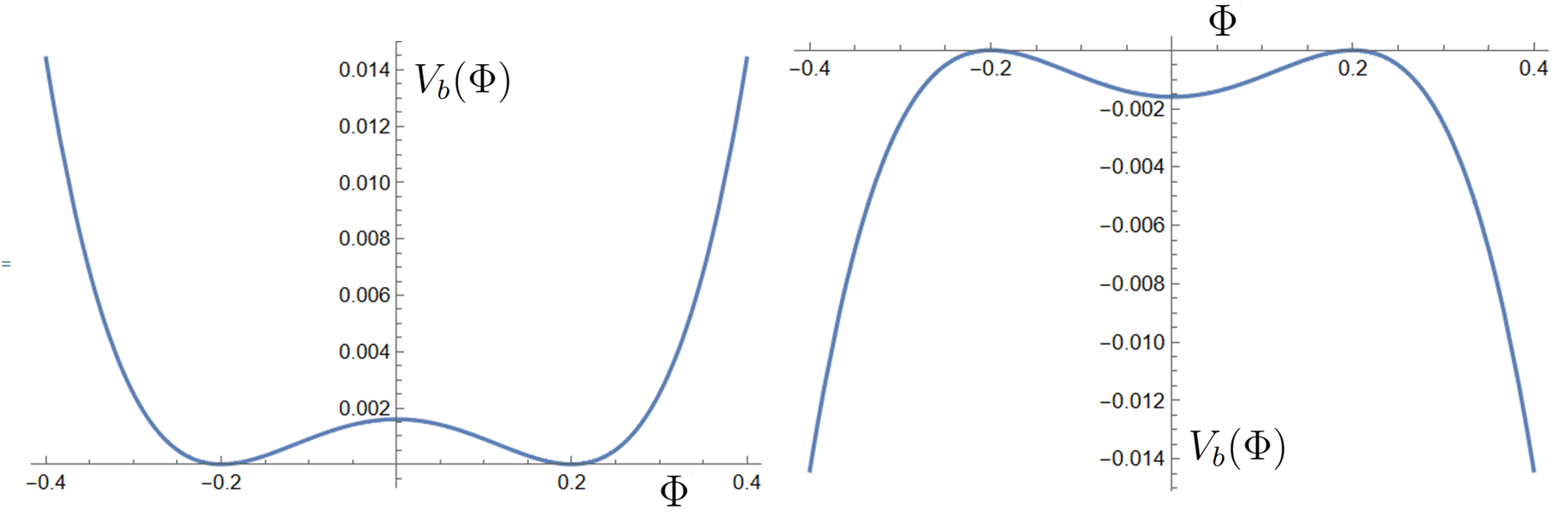
Figure 1: Form of the bulk potential $V_{b}(\Phi)$ with $b=0.2$ for $\lambda=1$ (left) and $\lambda=-1$ (right)

We again follow the CMS method for this more general form of bulk potential as the classical equation of motion for $\Phi$ is certainly difficult to solve analytically.

$$\partial^{2}_{\phi}\Phi-4kr_{c}\partial_{\phi}\Phi+4\lambda r_{c}^{2}\Phi(\Phi^{2}-b^{2})=0$$ (46)

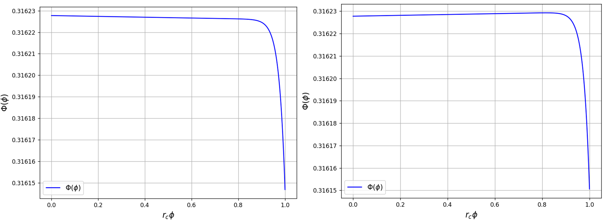
Figure 2: Scalar field profile for parameter values $b=0.2,v=0.01,k=10,\alpha=10^{-5}$ with $\lambda=0.001$ (left) and $\lambda=-0.001$ (right)

We use Eq.(23) to find the OR solution for $\Phi$ which takes the form

$$\Phi_{OR}(\phi)=\frac{b}{\sqrt{1-e^{2b^{2}(a\phi+d)}}}$$ (47)

where $a=-\frac{r_{c}\lambda}{k}$ and $d=\frac{1}{2b^{2}}\ln[1-\frac{b^{2}}{k^{3}v^{2}}]$. The integral constant ‘d’ is found out by using the boundary condition

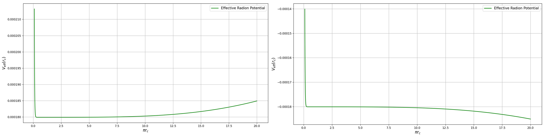
Figure 3: Effective radion potential for parameter values $b=0.2,v=0.01,k=10,\alpha=10^{-5}$ with $\lambda=0.001$ (left) and $\lambda=-0.001$ (right)

$\Phi(\phi=0)=k^{3/2}v$. Matching with the BR solution Eq.(25), we get the approximate solution for $\Phi$ as

$$\Phi_{approx}(\phi)=-\frac{k^{3/2}\alpha}{4}e^{4kr_{c}(\phi-\pi)}+\frac{b}{\sqrt{1-e^{2b^{2}(a\phi+d)}}}$$ (48)

Note that this solution is ill-defined when $a\phi+d=0$ which implies $r_{c}\phi=\frac{k}{2b^{2}\lambda}\ln[1-\frac{b^{2}}{k^{3}v^{2}}]$. Now, $(1-\frac{b^{3}}{k^{3}v^{2}})$ is certainly less than 1, k being positive, resulting in a negative value of $r_{c}$ which is unphysical. Thus, the solution is well defined along the entire positive $r_{c}$ (physical) axis. As with the original GW scheme, we fine-tune the brane tensions to make the gravitational contribution to the radion potential vanish. So, the only contribution is of the GW type. Hence, we take the scalar field profile given by Eq.(48) and plug it in Eq.(19) with the brane potentials:

$$V_{h} = \lambda_{h}(\Phi^{2}-k^{3}v^{2})^{2}$$ (49)

$$V_{v} = 2\alpha k^{5/2}\Phi$$ (50)

We then integrate over the extra dimension i.e. $\phi$ to get the expression for the effective radion potential. It is quite cumbersome to get the analytic expression. So, we resort to the numerical results (see Fig. 3) which do provide the necessary insights.

What we get is that the effective potential has a global minimum for a double well bulk potential i.e. the modulus gets stabilized to a non-trivial non-zero value, which for our benchmark choice of parameters in Fig. 3 turns out to be 0.31. As a result, $k\pi r_{c}\approx 31$ which very well solves the hierarchy problem. However, for the inverted double well, the modulus gets destabilized (no minimum). Thus, we get another example which hints at a one-one correspondence between both the stabilities.

IV.5 Bazeia-Furtado-Gomes type bulk potential

Bazeia, Furtado and Gomes (BFG); in [23], introduced a set of bulk scalar potentials which are generated from a class of superpotentials of the form

$$W_{p}(\Phi)=\frac{2p}{2p-1}\,\Phi^{\frac{2p-1}{p}}-\frac{2p}{2p+1}\,\Phi^{\frac{2p+1}{p}}$$ (51)

where p is an odd integer, and the bulk potential given by [taking $\kappa^{2}=2$]:

$$V_{p}(\Phi)=\frac{1}{8}\left(\frac{dW_{p}}{d\Phi}\right)^{2}-\frac{1}{3}W^{2}_{p}$$ (52)

The metric ansatz we use is

$$ds^{2}=e^{2A(y)}\eta_{\mu\nu}dx^{\mu}dx^{\nu}-dy^{2}$$ (53)

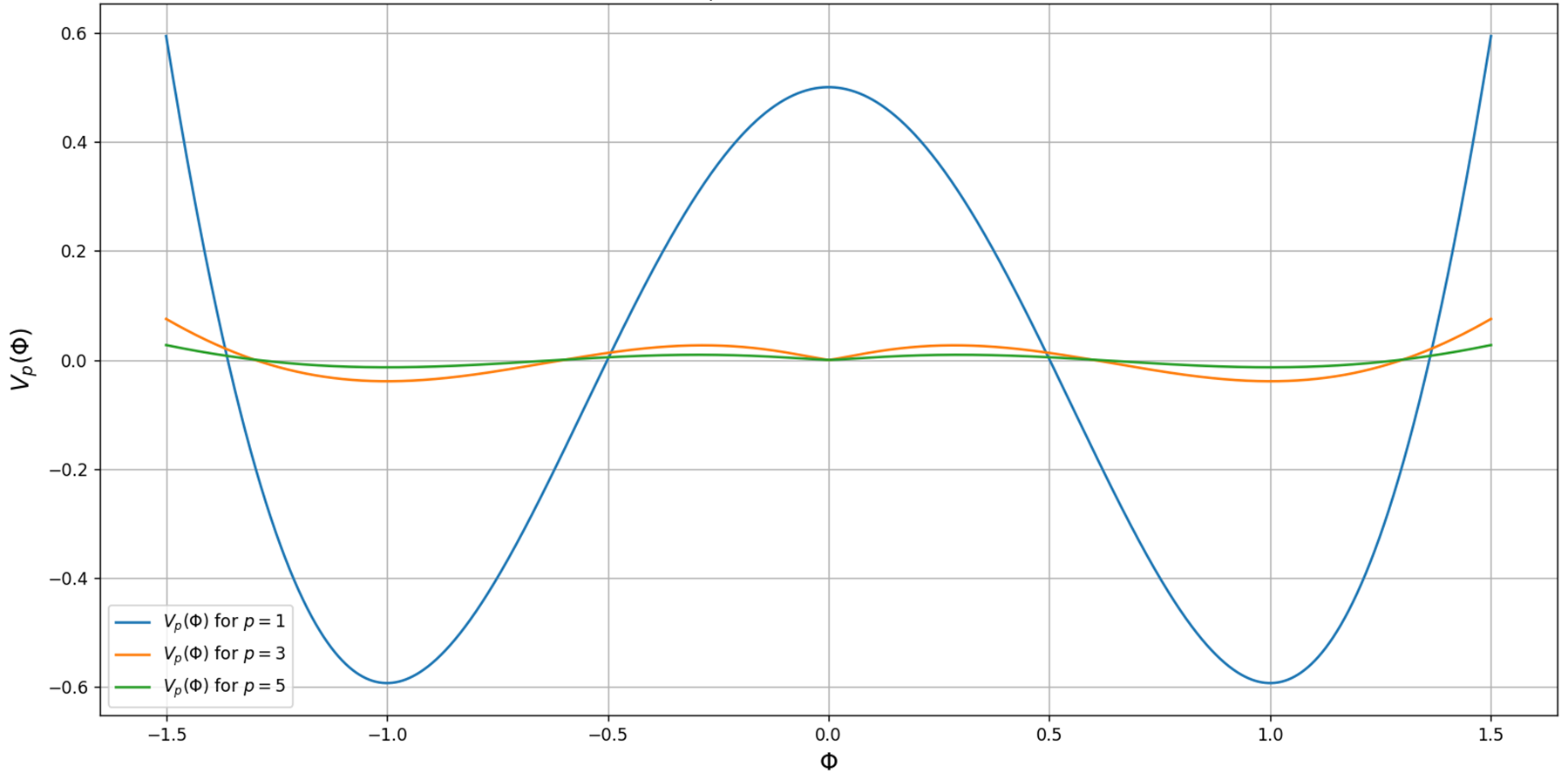
Figure 4: BFG potentials for different p values

The speciality of these potentials is that the coupled gravity-scalar system gives rise to thick brane solutions. What we do here is take such forms of bulk potentials and plug them in the RS-I background with proper brane potentials - hence solving for the scalar profile and backreacted metric using the superpotential approach of Ref. [4] (see Appendix A). The next step is to calculate the effective radion potential and check the behaviour for the entire class of superpotentials. A final question is if we can establish a relation between the value of the stabilized modulus ($r_{c}$) [if it gets stabilized] and the parameter p, which is addressed in Appendix B.

Following the steps as in Appendix A, we obtain the following solutions for the scalar profile and the warp factor [23]:

$$\Phi_{p}(y)=\tanh^{p}\left(\frac{y}{p}\right)$$

$$\begin{split}\noindent A_{p}(y)\!\!=\!\!-\frac{1}{3}\frac{p}{2p+1}\tanh^{2p}\left(\frac{y}{p}\right)-\frac{2}{3}\left(\frac{p^{2}}{2p-1}-\frac{p^{2}}{2p+1}\right)\\ \biggl{\{}\ln[\cosh\left(\frac{y}{p}\right)\biggr{]}-\sum_{n=1}^{p-1}\frac{1}{2n}\tanh^{2n}\left(\frac{y}{p}\right)\biggr{\}}\end{split}$$ (54)

One should notice that, unlike all the cases till now, this is an exact solution involving the backreaction. The additional inputs that we need to give are the brane potentials which are precisely determined by Eqs. (48) and (49). Hence, putting in the scalar field solution and modified warp factor into the combined gravity-scalar action, integrating over the extra dimension and adding the contribution due to brane potentials; we get the effective radion potential . In this scenario as well, the calculations are quite cumbersome to do analytically, especially when our sole purpose is to determine the presence of modulus stabilization. So, we resort to a numerical approach.

Figure 5: Effective radion potential for p = 1 (top left), p = 3 (top right) and p = 5 (bottom)

From Fig. 5, we see that one gets modulus stabilization for BFG type bulk scalar potentials at least for p till 19 which has been checked numerically - The computational resources required for the numerical calculations increase as the value of p increases. But, since the potentials for all further p values retain the same structure (see Fig. 5), we conjecture that one gets modulus stabilization for the entire class of BFG type bulk scalar potentials.

As the scalar field solution is a tan hyperbolic raised to an odd power, it has values between plus and minus one. This restricts the domain of the bulk potentials and hence, the bulk potentials are bounded from below by their values at $\pm 1$. Given the nature of our argument for all the cases till now, we would have naturally expected modulus stabilization in these scenarios which is indeed what we get.

IV.6 Mishra-Randall ansatz

Recently, Mishra and Randall [18] explored the effect of including bulk interaction terms for the GW scalar on RS cosmology. In particular, they were interested in the form of the beta function ($\beta=1/T$), where T is the

Figure 6: GW bulk potentials [($\epsilon_{2}<0,\epsilon_{3}<0$);($\epsilon_{2}<0,\epsilon_{3}>0$); ($\epsilon_{3}<0,\epsilon_{2}>0$); ($\epsilon_{2}>0,\epsilon_{3}>0$)]: from left to right

Figure 7: Radion potentials [($\epsilon_{2}<0,\epsilon_{3}<0$);($\epsilon_{2}<0,\epsilon_{3}>0$); ($\epsilon_{3}<0,\epsilon_{2}>0$); ($\epsilon_{2}>0,\epsilon_{3}>0$)]: from left to right

black hole temperature whose origin lies in its Hawking radiation. In the RS background, this function could take up any value. For no bulk interaction of the GW scalar, the beta function is a constant, and higher-order terms in the GW bulk potential correspond to higher-order terms in the beta function. With this in mind (to model the additional terms in beta), they considered an ansatz of the form:

$$V_{b}(\Phi)=2\epsilon_{2}\Phi^{2}+\frac{4}{3}\epsilon_{3}\Phi^{3}$$ (55)

The brane potentials that they consider are of the form

$$V_{hid}(\Phi)=\beta_{hid}(\Phi-v_{hid})^{2}\>,\;\>\beta_{hid}\to\infty\>,\\ \>V_{vis}(\Phi)=2\alpha_{vis}\Phi$$ (56)

The scalar field profile, as given by the CMS scheme is

$$\Phi_{\text{RS}}(r)=-\frac{\alpha_{vis}}{4}e^{4(r-r_{vis})}+\frac{v_{hid}e^{-\epsilon_{2}r}}{1+v_{hid}\epsilon_{3}\left(\frac{1-e^{-\epsilon_{2}r}}{\epsilon_{2}}\right)}$$ (57)

with $0\leq r\leq r_{vis}$. Plugging everything into the GW action and integrating over the fifth dimension gives the following form for the radion potential [18]

$$\begin{split}V(\varphi)=24M_{5}^{3}\kappa^{4}\,\varphi^{4}(1+\frac{a_{2}}{24M_{5}^{3}\kappa^{4}}\frac{\lambda\varphi^{\epsilon_{2}}}{1-\lambda\varphi^{\epsilon_{2}}}\\ -\frac{a_{3}}{24M_{5}^{3}\kappa^{4}}\,\log(1-\lambda\varphi^{\epsilon_{2}}))\end{split}$$ (58)

with

$$\begin{split}\qquad\varphi=e^{-r_{vis}},\>\lambda=\frac{v_{\text{hid}}\epsilon_{32}}{1+v_{\text{hid}}\epsilon_{32}},\>\epsilon_{32}=\frac{\epsilon_{3}}{\epsilon_{2}},\\ \>a_{2}=-\frac{1}{32}\epsilon_{2}\alpha_{vis}^{2}-\frac{\epsilon_{2}}{\epsilon_{3}}\alpha_{vis}+2\alpha_{vis},\\ \>a_{3}=\frac{1}{2}\frac{\epsilon_{2}}{\epsilon_{3}}\alpha_{vis}\end{split}$$ (59)

We now work with a specific choice of parameters, which was part of the benchmark choice in Ref.[18] as well: $\kappa=10^{-1/4},\epsilon_{2}=-1/25,\epsilon_{3}=-1/90,\alpha_{ir}=5/2,v_{uv}=1/5$. The resulting radion potential has a minimum at $0.86\>X\>10^{-16}$ corresponding to $r_{vis}\approx 36.98$ which certainly solves the hierarchy problem. Now, we work with the same magnitudes for $\epsilon_{2}$ and $\epsilon_{3}$ but with different sign combinations: namely one of $\epsilon_{2}$ or $\epsilon_{3}$ being positive or both being positive. In both cases, we do not get modulus stabilization as $r_{c}$ either vanishes or is driven to infinity. In the first case, we get a monotonically decreasing radion potential with a minimum at $\varphi=1$, corresponding to $r_{vis}=0$ and in the second case, the radion potential is monotonically increasing and hence, attains its minimum at $\varphi=0$ i.e. $r_{vis}\to\infty$ [see Figs. 6,7]. These results do not aid us in etching a correspondence between the two stabilities as we have done till now and may be linked to the fact that the bulk potentials here do not have a global minimum or maximum like the other cases.

We get modulus stabilization for the $\epsilon_{3}=0,\epsilon_{2}<0$ case as is shown in Ref.[18]. However, the interesting case is $\epsilon_{2}=0$ i.e. only cubic contribution. We see from Eq.(59) that in this limit, $a_{2}=2\alpha_{vis},a_{3}=0,\epsilon_{32}\to\infty$ and hence, $\lambda\to 1$. Plugging these in Eq.(58), we see that the third term becomes zero while the second term is non-zero but blows up. The most important thing to notice here is that as all the $\phi$ contributions within the brackets were raised to the power $\epsilon_{2}$, we are left with no $\phi$ dependance for the quartic coefficient now - it is a constant. Thus, the radion VEV is either zero or driven to infinity depending on the sign of this constant implying no modulus stabilization irrespective of the sign of $\epsilon_{3}$. This is certainly what we expected as this was our conclusion when we independently examined the cubic bulk potential GW scenario without the gravitational contributions. Thus, it serves as a good check that our results match under proper limits.

V Addressing the correspondence

Here, we discuss two classes of the GW bulk potential (the potential satisfying certain properties) that clearly indicate the one-one correspondence between GW scalar stability and successful modulus stabilization. It is worthwhile to note that the below proofs include some approximations and hence, we would be critical and say that the correspondence is not exact - rather the possibilty of it being valid is incredibly high.

V.1 Global minimum for $V_{b}(\Phi)$

The existence of a global minimum for the bulk scalar potential has strong implications for the OR solution of $\Phi$ (see Eq.23). Particularly, the OR equation of Eq.(23) indicates the existence of a stable fixed point for $\Phi_{OR}$ at $\Phi_{0}$ - the scalar field value at which $V_{b}(\Phi)$ attains its global minimum. As a result, the profile of $\Phi_{OR}$ is such that it gets a lot of contribution from the global minimum well, around $\Phi_{0}$. This allows us to treat the bulk potential as an expansion around its minimum. As we are interested in the nature of the potential, we can take the global minimum at the origin i.e. $\Phi_{0}=0$ and $V(\Phi_{0})=0$. The rescaling essentially implies corrections to the bulk cosmological constant which is assumed to still remain negative ($AdS_{5}$). We alternatively call $V_{b}(\Phi)$ as $V(\Phi)$ and $V_{b}^{\prime\prime}(\Phi)|_{\Phi=\Phi_{0}}$ as $V^{\prime\prime}$ for brevity.

$$V(\Phi)=V(\Phi_{0})+\frac{1}{2}V^{\prime\prime}(\Phi)|_{\Phi=\Phi_{0}}(\Phi-\Phi_{0})^{2}=\frac{1}{2}V^{\prime\prime}(\Phi)|_{\Phi=\Phi_{0}}\Phi^{2}$$ (60)

neglecting the higher order terms. Note that $V^{\prime\prime}\geq 0$ as it is a minimum but for this proof, we restrict to $V^{\prime\prime}>0$. In the discussion below, by “conditions”, we mean boundary conditions and brane couplings.

V.1.1 GW conditions

With GW conditions [as defined in Sec.II(C)], the analysis is exactly the same as Sec.II(C) except $V^{\prime\prime}(\Phi)|_{\Phi=\Phi_{0}}$ representing the squared mass of the bulk scalar. Hence, we get modulus stabilization.

Under GW conditions, if the bulk scalar potential has a global minimum satisfying $V^{\prime\prime}>0$, then it implies modulus stabilization.

V.1.2 CMS conditions

We write the OR solution as

$$\Phi_{OR}=\Phi_{0}+\epsilon(\phi)=\epsilon(\phi)$$ (61)

Plugging these expressions into the OR equation $\frac{d\Phi_{OR}}{d\phi}=-\frac{r_{c}}{4k}V^{\prime}(\Phi)$, we get the following solution for $\Phi_{OR}$,

$$\Phi_{OR}(\phi)=\epsilon_{0}e^{-r_{c}V^{\prime\prime}\phi/4k}$$ (62)

with $\epsilon_{0}$ being the integration constant which is determined by the boundary condition $\Phi(0)=k^{3/2}v$. Finally, combining with the BR solution, the resulting scalar field profile is given by

$$\Phi(\phi)=-\frac{k^{3/2}\alpha}{4}e^{4kr_{c}(\phi-\pi)}+k^{3/2}ve^{-r_{c}V^{\prime\prime}\phi/4k}$$ (63)

The GW part of the radion potential is obtained by using this solution in Eq.(19) with the choice for visible brane potential determined by Eq.(20).

$$\begin{split}V(r_{c})=\frac{k^{4}\alpha^{2}}{4}e^{-8kr_{c}\pi}(e^{4kr_{c}\pi}-1)\\ -\frac{(V^{\prime\prime})^{2}}{8k}\frac{k^{3}v^{2}}{V^{\prime\prime}+8k^{2}}(e^{-(\frac{r_{c}V^{\prime\prime}}{2k}+4kr_{c})\pi}-1)\\ -k^{4}\alpha ve^{-4kr_{c}\pi}(e^{-r_{c}V^{\prime\prime}\pi/4k}-1)\\ -2k^{4}v^{2}\frac{V^{\prime\prime}}{V^{\prime\prime}+8k^{2}}(e^{-(\frac{r_{c}V^{\prime\prime}}{2k}+4kr_{c})\pi}-1)\\ -\frac{k^{4}\alpha^{2}}{2}e^{-4kr_{c}\pi}+2k^{4}\alpha ve^{-(\frac{r_{c}V^{\prime\prime}}{4k}+4kr_{c})\pi}\end{split}$$ (64)

We now calculate the derivatives of the radion potential,

$$\begin{split}V^{\prime}(r_{c})=k^{5}\alpha^{2}\pi e^{-4kr_{c}\pi}-4k^{5}\alpha\pi ve^{-4kr_{c}\pi}+2k^{5}\alpha^{2}\pi e^{-8kr_{c}\pi}\\ +\frac{k\pi}{16}v^{2}(V^{\prime\prime})^{2}e^{-(\frac{r_{c}V^{\prime\prime}}{2k}+4kr_{c})\pi}+k^{4}\alpha\pi v(4k+\frac{V^{\prime\prime}}{4k})e^{-(\frac{r_{c}V^{\prime\prime}}{4k}+4kr_{c})\pi}\\ +k^{3}v^{2}\pi V^{\prime\prime}e^{-(\frac{r_{c}V^{\prime\prime}}{2k}+4kr_{c})\pi}-2\alpha k^{4}v\pi(\frac{V^{\prime\prime}}{4k}+4k)e^{-(\frac{r_{c}V^{\prime\prime}}{4k}+4kr_{c})\pi}\end{split}$$ (65)

The fact that $4kr_{c}>>1$ allows us to neglect the $e^{-8kr_{c}\pi}$ term. At the extremum (supposing it exists) say $r_{c}^{*}$, Eq.(65) vanishes. The second derivative of the radion potential at extremum $r_{c}^{*}$ is then given by

$$\begin{split}V^{\prime\prime}(r_{c})|_{r_{c}^{*}}=\frac{k^{2}\pi^{2}\alpha v}{16}V^{\prime\prime}(V^{\prime\prime}+16k^{2})e^{-(\frac{r_{c}V^{\prime\prime}}{4k}+4kr_{c})\pi}\end{split}$$ (66)

where we have dropped $\mathcal{O}(e^{-(\frac{r_{c}V^{\prime\prime}}{2k}+4kr_{c})\pi})$ terms in favour of $\mathcal{O}(e^{-(\frac{r_{c}V^{\prime\prime}}{4k}+4kr_{c})\pi})$ terms and used the fact that Eq.(65) vanishes at $r_{c}^{*}$. As $V^{\prime\prime}>0$, we can see that Eq.(66) is strictly positive as long as $\alpha v>0$ (we can always impose this by boundary conditions). Thus, the extremum is surely a minimum.

Under CMS conditions, if the bulk scalar potential has a global minimum satisfying $V^{\prime\prime}>0$ and the corresponding radion potential has an extremum for a positive value of $r_{c}$, then the extremum is certainly a minimum of the radion potential, implying modulus stabilization.

V.2 Global maximum but no global minimum for $V_{b}(\Phi)$

The analysis follows as same except now, the perturbative solution for the scalar field is a runaway solution as the point of maximum is an unstable fixed point of the system and there exists no global minimum. The bulk potential can be approximated as same except $V^{\prime\prime}\leq 0$ - for the proof, we take it to be $V^{\prime\prime}<0$.

V.2.1 GW conditions

The analysis is as given in Sec.IV(A). We deal with a negative mass term which essentially results in modulus destabilization as we showed previously.

Under GW conditions, if the bulk scalar potential has a global maximum satisfying $V^{\prime\prime}>0$, then the corresponding radion potential has no extremum for a positive value of $r_{c}$ implying no modulus stabilization.

V.2.2 CMS conditions

$V^{\prime\prime}>0$ allows us to only consider the terms involving $e^{-\frac{r_{c}V^{\prime\prime}\pi}{4k}}$ and $e^{-\frac{r_{c}V^{\prime\prime}\pi}{2k}}$ in Eq.(65) as they are increasing exponentials, $V^{\prime\prime}$ being negative. Supposing the extremum exists, then the second derivative of the radion potential at the extremum $r_{c}^{*}$ is given by

$$V^{\prime\prime}(r_{c})|_{r_{c}^{*}}=-\frac{k^{2}\pi^{2}\alpha v}{8}V^{\prime\prime}(V^{\prime\prime}+16k^{2})e^{-(\frac{r_{c}V^{\prime\prime}}{4k}+4kr_{c})\pi}$$ (67)

where we have used the vanishing of the first derivative at extremum. $V^{\prime\prime}$ being negative and ensuring $\alpha v>0$ as in the previous proof, we have two cases: (a) $V^{\prime\prime}<-16k^{2}$ indicates a maximum and (b) $-16k^{2}<V^{\prime\prime}<0$ indicates a minimum. Thus we get to the following theorem,

Under CMS conditions, if the bulk scalar potential has a global maximum but no global minimum, and the corresponding radion potential has an extremum for a positive value of $r_{c}$, then the extremum is a maximum of the radion potential if $V^{\prime\prime}<-16k^{2}$ or a minimum of the radion potential if $-16k^{2}<V^{\prime\prime}<0$ implying modulus destabilization or stabilization respectively.

Though the $V^{\prime\prime}=0$ case was not included here, we suspect that the above results hold for such scenarios as well. The case study of Sec.IV(C) supports this belief.

Thus, from these, we can conclude that if the bulk GW potential has a global minimum, then modulus stabilization is guaranteed. However, for GW bulk potentials with a global maximum and no global minimum, we saw that modulus stabilization may or may not be achieved depending on the choice of our parameters for the bulk potential. Note that these deductions are consistent with but do not explain the case studies for bulk cubic interaction and the Mishra-Randall ansatz.

It must be noted that we went for a full expansion of the radion potential for the CMS proofs unlike Ref.[5] which calculates only to the leading order in $v$ albeit incorporating gravitational sector contribution.

VI Criteria for bulk potential to ensure modulus stabilization

In this section, we will frequently use tools from Sec. III. Firstly, note that for a general bulk scalar potential $V(\Phi)$ and defining $z=r_{c}\phi$, the general scalar solution is given by

$$\Phi(z)=\Phi_{BR}(z)+\Phi_{OR}(z)=-\frac{k^{3/2}\alpha}{4}e^{4k(z-\pi r_{c})}+\Phi_{OR}(z)$$ (68)

Using the OR equation, we can now write

$$\begin{split}\partial_{z}\Phi|_{\pi r_{c}}=-k^{5/2}\alpha-\frac{V^{\prime}(\Phi_{OR})|_{\pi r_{c}}}{4kr_{c}}\\ \partial_{z}V(\Phi)|_{\pi r_{c}}=V^{\prime}(\Phi)|_{\pi r_{c}}(-k^{5/2}\alpha-\frac{V^{\prime}(\Phi_{OR})|_{\pi r_{c}}}{4kr_{c}})\end{split}$$

We write $V^{\prime}(\Phi)|_{\pi r_{c}}$ as $V^{\prime}(\Phi)$ and $V^{\prime}(\Phi_{OR})|_{\pi r_{c}}$ as $V^{\prime}(\Phi_{OR})$ for brevity. Then, plugging these along with the brane potentials defined in Sec.III into Eq.(19), applying Leibniz’s rule to get the first derivative of the radion potential $U(r_{c})$ and setting it to zero (we demand the existence of an extremum at $r_{c}^{*}$) gives us the following relation evaluated at $r_{c}^{*}$

$$\begin{split}\frac{\pi}{2}k^{5}\alpha^{2}+\frac{\pi(V^{\prime}(\Phi_{OR}))^{2}}{32k^{2}r_{c}^{*2}}+\frac{\pi k^{3/2}\alpha V^{\prime}(\Phi_{OR})}{4r_{c}^{*}}-\pi k^{5/2}\alpha V^{\prime}(\Phi)\\ -\frac{\pi V^{\prime}(\Phi)V^{\prime}(\Phi_{OR})}{4kr_{c}^{*}}+2\pi\alpha^{2}k^{5}-8\alpha\pi k^{7/2}\Phi_{OR}(\pi r_{c}^{*})\\ +2\alpha k^{5/2}\frac{d\Phi_{OR}(\pi r_{c})}{dr_{c}}|_{r_{c}^{*}}=0\end{split}$$ (69)

$\Phi_{OR}(\pi r_{c})$ is small as the outer region solution is suppressed at the boundary and $V^{\prime}(\Phi)$ is assumed to be small at the boundary as per the CMS scheme. Thus, the terms $V^{\prime}(\Phi)$ and $V^{\prime}(\Phi_{OR})$ are small and we ignore their quadratics. This reduces Eq.(69) to

$$\frac{5}{2}\alpha k^{7/2}+\frac{V^{\prime}(\Phi_{OR})}{4r_{c}^{*}}-kV^{\prime}(\Phi)-8k^{2}\Phi_{OR}(\pi r_{c})+2k\Phi_{OR}^{\prime}(\pi r_{c})=0$$ (70)

We now evaluate $U^{\prime\prime}(r_{c})$ at $r_{c}^{*}$.

$$\begin{split}U^{\prime\prime}(r_{c})|_{r_{c}^{*}}=e^{-4kr_{c}^{*}\pi}[\frac{V^{\prime\prime}(\Phi_{OR})}{4r_{c}^{*}}.\frac{d\Phi_{OR}(\pi r_{c})}{dr_{c}}\\ -kV^{\prime\prime}(\Phi)\frac{d\Phi(\pi r_{c})}{dr_{c}}-8k^{2}\frac{d\Phi_{OR}(\pi r_{c})}{dr_{c}}\\ +\frac{2k}{\pi}\frac{d^{2}\Phi_{OR}(\pi r_{c})}{dr_{c}^{2}}-\frac{1}{4r_{c}^{*2}}V^{\prime}(\Phi_{OR})]\end{split}$$ (71)

It should be remembered that the derivatives in the above expression are all evaluated at $r_{c}^{*}$. Also, from Eq.(68), we see that $\frac{d\Phi(\pi r_{c})}{dr_{c}}=\frac{d\Phi_{OR}(\pi r_{c})}{dr_{c}}$. To ensure positivity of the radion mass and modulus stabilization, Eq.(71) must be positive which results in the following criterion

$$\begin{split}\frac{2k}{\pi}\frac{d^{2}\Phi_{OR}(\pi r_{c})}{dr_{c}^{2}}|_{r_{c}^{*}}>[8k^{2}+kV^{\prime\prime}(\Phi)|_{r_{c}^{*}}\\ -\frac{V^{\prime\prime}(\Phi_{OR})|_{r_{c}^{*}}}{4r_{c}^{*}}]\frac{d\Phi_{OR}(\pi r_{c})}{dr_{c}}|_{r_{c}^{*}}+\frac{1}{4r_{c}^{*2}}V^{\prime}(\Phi_{OR})|_{r_{c}^{*}}\end{split}$$ (72)

Using Eq.(70) to substitute $\frac{d\Phi_{OR}(\pi r_{c})}{dr_{c}}|_{r_{c}^{*}}$ in Eq.(72), we get the expression

$$\begin{split}(\frac{2k}{\pi})^{2}\frac{d^{2}\Phi_{OR}(\pi r_{c})}{dr_{c}^{2}}|_{r_{c}^{*}}>[8k^{2}+kV^{\prime\prime}(\Phi)-\frac{V^{\prime\prime}(\Phi_{OR})}{4r_{c}^{*}}]\\ [kV^{\prime}(\Phi)+8k^{2}\Phi_{OR}(\pi r_{c}^{*})-\frac{V^{\prime}(\Phi_{OR})}{4r_{c}^{*}}-\frac{5}{2}\alpha k^{7/2}]\\ +\frac{k}{2\pi r_{c}^{*2}}V^{\prime}(\Phi_{OR})\end{split}$$ (73)

where on the right hand side, the “evaluated at $r_{c}^{*}$” is implicit. As one can see, the Eqs.(70) and (73) are completely determined by the bulk scalar potential (note that $\Phi(z)$ depends only on $V^{\prime}(\Phi)$). Thus, these are the two relations that any general bulk potential must satisfy in order for the radion potential to have a stable minimum. It should again be noted that these results hold under our assumed boundary conditions.

We did a quick check for the case with no bulk interaction i.e. $V(\Phi)=\frac{1}{2}m^{2}\Phi^{2}$ with a set of parameters for which modulus stabilization is possible (see Eq.(2.22), [5]): $\alpha=0.2,k=1,v=0.05,\epsilon=\frac{m^{2}}{4k^{2}}=0.5$. This satisfies Eqs.(70) and (73) with $r_{c}^{*}=1.156$. Similarly, one can do the checking for other potentials but these relations are guaranteed to hold as they are derived generally.

VII Conclusion

Our analysis brings out a deep correlation between the stability of the scalar field (which has been employed for modulus stabilization) and the corresponding existence of a stable minimum for the modulus. The outcomes can be summarized as follows: (1) Existence of a global minimum for the scalar sector immediately ensures a stable minimum for the modulus. (2) On the contrary, the scalar sector which does not have a global minimum may or may not lead to modulus stabilization. It is to be noted that the results are subject to the two types of boundary conditions that we assumed. (3) Our calculations addressed various scalar field actions to explore the resulting stabilization of the moduli sector. This included a canonical kinetic term as well as phantom like term for the scalar sector. Moreover, choosing different forms of the scalar field potentials, we carefully examined the possibility of a corresponding modulus stabilization. (4) It may further be observed that such different stabilizing scalar sectors in the scalar-tensor models have direct correspondence with higher curvature gravity models and thus, our calculations indirectly include various viable f(R) models which may lead to modulus stabilization. The results therefore provide us with a powerful tool to test modulus stabilization for different bulk stabilizing fields.

Appendix A Including backreaction - The Superpotential Method

In GW scenarios, we neglected the back-reaction of the metric to the presence of the scalar field in the bulk but this is important indeed and therefore, it would be very nice to simultaneously solve the Einstein and the bulk scalar equations, to have the back-reaction exactly under control. DeWolfe et al. [4] provides us with such a formalism. Denote the scalar field in the bulk by $\Phi$, and consider the action

$$\begin{split}\int d^{5}x\sqrt{g}\left[-M^{3}R++\frac{1}{2}(\nabla\Phi)^{2}-V(\Phi)\right]\\ -\int d^{4}x\sqrt{g_{4}}\lambda_{hid}(\Phi)-\int d^{4}x\sqrt{g_{4}}\lambda_{vis}(\Phi)\end{split}$$ (74)

We look for an ansatz of the background metric again of the generic form as in the RS case to maintain 4D Lorentz invariance:

$$ds^{2}=e^{-2A(y)}\eta_{\mu\nu}dx^{\mu}dx^{\nu}-dy^{2}$$ (75)

Using this metric, we get the Einstein equations and bulk scalar equation of the form

$$4A^{\prime 2}-A^{\prime\prime} =-\frac{2\kappa^{2}}{3}V(\Phi_{0})-\frac{\kappa^{2}}{3}\sum_{i=vis,hid}\lambda_{i}(\Phi_{0})\delta(y-y_{i}),$$ (76)

$$A^{\prime 2} =\frac{\kappa^{2}}{12}\Phi_{0}^{\prime 2}-\frac{\kappa^{2}}{6}V(\Phi_{0}),$$ (77)

$$\Phi_{0}^{\prime\prime}-4A^{\prime}\Phi_{0}^{\prime} =\frac{\partial V}{\partial\Phi_{0}}+\sum_{i}\frac{\partial\lambda_{i}(\Phi_{0})}{\partial\Phi}\delta(y-y_{i}).$$ (78)

The jump conditions at the branes are then given by

$$[A^{\prime}]_{i}=\frac{\kappa^{2}}{3}\lambda_{i}(\Phi_{0})$$

$$[\Phi_{0}^{\prime}]_{i}=\frac{\partial\lambda_{i}(\Phi_{0})}{\partial\Phi}$$ (79)

The bulk equations Eqs. (76-78) along with the boundary conditions Eq. (A) form the coupled gravity-scalar system. We can now define the function $W(\Phi)$ via the equations

$$A^{\prime}\equiv\frac{\kappa^{2}}{6}W(\Phi_{0})$$

$$\Phi_{0}^{\prime}\equiv\frac{1}{2}\frac{\partial W}{\partial\Phi}$$ (80)

Plugging in these expressions into the bulk equations, we find that all the equations are satisfied simultaneously if the following consistency criterion holds,

$$V(\Phi)=\frac{1}{8}\left(\frac{\partial W}{\partial\Phi}\right)^{2}-\frac{\kappa^{2}}{6}W(\Phi)^{2}$$ (81)

The jump conditions translate to:

$$\frac{1}{2}[W(\Phi_{0})]_{i}=\lambda_{i}(\Phi_{0})$$

$$\frac{1}{2}[\frac{\partial W}{\partial\Phi}]_{i}=\frac{\partial\lambda_{i}(\Phi_{0})}{\partial\Phi}$$ (82)

Thus, we see that that the coupled second order differential equations now reduce to ordinary first order equations. The difficulty one has to entail is to find the superpotential $W(\Phi)$ given the potential $V(\Phi)$ which generally is a hard task. However, if we only need a superpotential which produces a family of potentials with some very general properties, then this prescription certainly simplifies our working.

Appendix B A relation between $r_{c}$ and p for the BFG case

Given that we take our conjecture holds true that there is indeed modulus stabilization for all BFG type potentials, a natural question to ask is whether we can establish some relation between $r_{c}$ and the only parameter in the problem p. We listed down all known $r_{c}$ values till p = 19, plotted $r_{c}$ vs p and found the empirical expression which best-fits the curve as

$$\pi r_{c}=ap^{1/b}+c$$ (83)

with a = 1.16, b = 0.82 and c = -0.69.

References

- Randall and Sundrum [1999] L. Randall and R. Sundrum, Large mass hierarchy from a small extra dimension, Phys. Rev. Lett. 83, 3370 (1999).
- Goldberger and Wise [1999] W. D. Goldberger and M. B. Wise, Modulus stabilization with bulk fields, Phys. Rev. Lett. 83, 4922 (1999).
- Goldberger and Wise [2000] W. D. Goldberger and M. B. Wise, Phenomenology of a stabilized modulus, Physics Letters B 475, 275 (2000).
- DeWolfe et al. [2000] O. DeWolfe, D. Z. Freedman, S. S. Gubser, and A. Karch, Modeling the fifth dimension with scalars and gravity, Phys. Rev. D 62, 046008 (2000).
- Chacko et al. [2013] Z. Chacko, R. K. Mishra, and D. Stolarski, Dynamics of a stabilized radion and duality, J. High Energy Phys. 2013.
- Chacko et al. [2015] Z. Chacko, R. K. Mishra, D. Stolarski, and C. B. Verhaaren, Interactions of a stabilized radion and duality, Phys. Rev. D 92, 056004 (2015).
- Csáki et al. [2001] C. Csáki, M. L. Graesser, and G. D. Kribs, Radion dynamics and electroweak physics, Phys. Rev. D 63, 065002 (2001).
- Lesgourgues and Sorbo [2004] J. Lesgourgues and L. Sorbo, Goldberger-wise variations: Stabilizing brane models with a bulk scalar, Phys. Rev. D 69, 084010 (2004).
- Anand et al. [2015] S. Anand, D. Choudhury, A. A. Sen, and S. SenGupta, Geometric approach to modulus stabilization, Phys. Rev. D 92, 026008 (2015).
- Das et al. [2008] S. Das, D. Maity, and S. SenGupta, Cosmological constant, brane tension and large hierarchy in a generalized randall-sundrum braneworld scenario, Journal of High Energy Physics 2008, 042 (2008).
- Dey et al. [2007] A. Dey, D. Maity, and S. SenGupta, Critical analysis of goldberger-wise stabilization of the randall-sundrum braneworld scenario, Phys. Rev. D 75, 107901 (2007).
- Das et al. [2018] A. Das, H. Mukherjee, T. Paul, and S. SenGupta, Radion stabilization in higher curvature warped spacetime, The European Physical Journal C 78, 10.1140/epjc/s10052-018-5603-9 (2018).
- Paul [2017] T. Paul, ”brane localized energy density” stabilizes the modulus in higher dimensional warped spacetime (2017), arXiv:1702.03722 [hep-th] .
- Banerjee et al. [2021] I. Banerjee, T. Paul, and S. SenGupta, Critical analysis of modulus stabilization in a higher dimensional gravity, Phys. Rev. D 104, 104018 (2021).
- Banerjee and SenGupta [2017] I. Banerjee and S. SenGupta, Modulus stabilization in a non-flat warped braneworld scenario, The European Physical Journal C 77, 10.1140/epjc/s10052-017-4857-y (2017).
- Das et al. [2017] A. Das, D. Maity, T. Paul, and S. SenGupta, Bouncing cosmology from warped extra dimensional scenario, Eur. Phys. J. C 77, 813 (2017), arXiv:1706.00950 [hep-th] .
- Banerjee et al. [2019] I. Banerjee, S. Chakraborty, and S. SenGupta, Radion induced inflation on nonflat brane and modulus stabilization, Phys. Rev. D 99, 023515 (2019).
- Mishra and Randall [2023] R. K. Mishra and L. Randall, Consequences of a stabilizing field’s self-interactions for rs cosmology, Journal of High Energy Physics 2023, 10.1007/jhep12(2023)036 (2023).
- Milton et al. [2002] K. A. Milton, S. D. Odintsov, and S. Zerbini, Bulk versus brane running couplings, Phys. Rev. D 65, 065012 (2002).
- Brevik et al. [2001] I. Brevik, K. A. Milton, S. Nojiri, and S. D. Odintsov, Quantum (in)stability of a brane-world universe at nonzero temperature, Nuclear Physics B 599, 305–318 (2001).
- Bender and Orszag [2010] C. M. Bender and S. A. Orszag, Advanced mathematical methods for scientists and engineers I (Springer, New York, NY, 2010).
- Breitenlohner and Freedman [1982] P. Breitenlohner and D. Z. Freedman, Stability in Gauged Extended Supergravity, Annals Phys. 144, 249 (1982).
- Bazeia et al. [2004] D. Bazeia, C. Furtado, and A. R. Gomes, Brane structure from a scalar field in warped spacetime, Journal of Cosmology and Astroparticle Physics 2004 (02), 002.
- Arkani–Hamed et al. [1998] N. Arkani–Hamed, S. Dimopoulos, and G. Dvali, The hierarchy problem and new dimensions at a millimeter, Physics Letters B 429, 263 (1998).
- Csaki [2004] C. Csaki, Tasi lectures on extra dimensions and branes (2004), arXiv:hep-ph/0404096 [hep-ph] .
- Rubakov [2001] V. A. Rubakov, Large and infinite extra dimensions, Physics-Uspekhi 44, 871–893 (2001).
- Sundrum [2005] R. Sundrum, Tasi 2004 lectures: To the fifth dimension and back (2005), arXiv:hep-th/0508134 [hep-th] .
- Das et al. [2016] A. Das, T. Paul, and S. SenGupta, Modulus stabilisation in a backreacted warped geometry model via goldberger-wise mechanism (2016), arXiv:1609.07787 [hep-ph] .
- Koley et al. [2009] R. Koley, J. Mitra, and S. SenGupta, Modulus stabilization of the generalized randall-sundrum model with a bulk scalar field, Europhysics Letters 85, 41001 (2009).