Abstract

Estimating the Kullback–Leibler (KL) divergence between language models has many applications, e.g., reinforcement learning from human feedback (RLHF), interpretability, and knowledge distillation. However, computing the exact KL divergence between two arbitrary language models is intractable. Thus, practitioners often resort to the use of sampling-based estimators. While it is easy to fashion a simple Monte Carlo (MC) estimator that provides an unbiased estimate of the KL divergence between language models, this estimator notoriously suffers from high variance, and can even result in a negative estimate of the KL divergence, a non-negative quantity. In this paper, we introduce a Rao–Blackwellized estimator that is also unbiased and provably has variance less than or equal to that of the standard Monte Carlo estimator. In an empirical study on sentiment-controlled fine-tuning, we show that our estimator provides more stable KL estimates and reduces variance substantially in practice. Additionally, we derive an analogous Rao–Blackwellized estimator of the gradient of the KL divergence, which leads to more stable training and produces models that more frequently appear on the Pareto frontier of reward vs. KL compared to the ones trained with the MC estimator of the gradient.

https://github.com/rycolab/kl-rb

1 Introduction

The Kullback–Leibler (KL; Kullback and Leibler, 1951) divergence is a statistical divergence that quantifies how one probability distribution differs from another. Measuring the KL divergence between probability distributions is a well-established problem that has been studied extensively in the statistics literature (Csiszár, 1967; Gibbs and Su, 2002, inter alia). In some special cases, e.g., in the case that we wish to measure the KL divergence between two Gaussian measures, the KL divergence has an analytical solution. However, in the general case, exact computation of the KL divergence is not analytically tractable or approximable with an efficient algorithm (Hershey and Olsen, 2007). This paper treats the case of computing the KL divergence between two language models (LMs), a fundamental task in natural language processing with numerous practical applications.

• In reinforcement learning from human feedback (RLHF Christiano et al., 2017; Stiennon et al., 2020; Ouyang et al., 2022) the KL divergence serves as a regularization term that constrains the distance between the language model and a reference model, typically the language model prior to fine-tuning. Specifically, constraining the KL divergence from the reference model prevents reward over-optimization and ensures that the model retains fluency while incorporating feedback from humans. Importantly, optimizing the RLHF objective needs more than just estimating the KL divergence; we also need to estimate its gradient with respect to the model’s parameters.

• In research on the interpretability of neural language models, the KL divergence is used to quantify how a specific prompt affects the language model conditioned on the prompt, e.g., researchers have applied the KL divergence between the model’s distribution before and after prompting the model in a controlled fashion (Pezeshkpour, 2023; Du et al., 2024a; Stoehr et al., 2024).

• As an evaluation metric, the KL divergence between the two language models serves as a metric for how well a neural language model has learned a target distribution. For example, Borenstein et al. (2024) and Svete et al. (2024) assess the learnability of probabilistic finite-state automata by measuring the KL divergence between a neural language model and the target distribution defined by the automata. Another example is evaluating language models after fine-tuning for human preference alignment, where we expect the model to stay close to the reference model (Rafailov et al., 2023).

• In knowledge distillation, when training a student language model to approximate a teacher model, minimizing the divergence between their distribution is a common objective, e.g., Agarwal et al. (2024) optimize a token-level application of the KL divergence for this purpose.

The points above demonstrate that measuring the KL divergence between two language models is useful and widespread. However, in the case of neural language models, it is far from straightforward. It is easy to see why: Given an alphabet of symbols $\Sigma$ and two language models $p$ and $q$, distributions over $\Sigma^{*}$, the KL divergence is given by the following expression

$$\textsc{kl}(p\mid\mid q)=\sum_{\boldsymbol{y}\in\Sigma^{*}}p(\boldsymbol{y})\log\frac{p(\boldsymbol{y})}{q(\boldsymbol{y})}\geq 0.$$ (1)

Recalling that $\Sigma^{*}$ is a countably infinite set, we cannot expect, in general, to compute Eq. 1 exactly in finite time without additional assumptions. While in some very special cases, e.g., where $p$ and $q$ are deterministic finite-state automata, there exist efficient algorithms, (Lehmann, 1977; Li and Eisner, 2009; Borenstein et al., 2024), we should not expect such an algorithm to exist in the case where $p$ and $q$ are neural language models, e.g., those based on the transformer (Vaswani et al., 2017; Radford et al., 2019; Meta, 2023). Thus, most researchers turn to approximation. A popular form of approximation resorts to stochastic approximation through Monte Carlo.

The naive Monte Carlo estimator for KL divergence (Eq. 1) involves sampling $M$ strings $\boldsymbol{Y}^{(1)},\ldots,\boldsymbol{Y}^{(M)}\mathrel{\stackrel{{\scriptstyle\textnormal{i.i.d.}}}{{\sim}}}p$ and then averaging $\log\frac{p(\boldsymbol{Y}^{(m)})}{q(\boldsymbol{Y}^{(m)})}$. Even though this estimator is unbiased, it often exhibits high variance. More pathologically, the naive Monte Carlo estimator can result in negative estimates of KL, which may be undesirable in practice. To address these issues, practitioners adopt alternative techniques to ensure non-negativity. For example, Schulman (2020) proposes an unbiased, non-negative KL estimator that is widely used in practice (von Werra et al., 2020; Havrilla et al., 2023). However, it offers no theoretical variance improvement over the Monte Carlo estimator and, as we show empirically, can exhibit unbounded variance.

In this paper, we derive an improved estimator of KL using Rao–Blackwellization (Gelfand and Smith, 1990; Casella and Robert, 1996), a well-established variance reduction technique from statistics. This results in an estimator that is provably unbiased and has a variance that is always less than or equal to that of the standard Monte Carlo estimator, while requiring no additional computational overhead. As a point of comparison to our Rao–Blackwellized estimator, we also provide a comprehensive formal analysis of various existing methods for estimating KL divergence, examining their bias and variance.

We empirically validate our theoretical findings using the well-established sentiment-controlled generation task (Rafailov et al., 2023) as a testbed. Specifically, we measure the KL divergence between a GPT-2 model (Radford et al., 2019) before and after fine-tuning, where the fine-tuning objective is to steer the model toward generating positive movie reviews. Our experimental results confirm that the Rao–Blackwellized estimator significantly reduces the variance of the Monte Carlo estimator, yielding the most stable and reliable estimates among all methods studied. In contrast, alternative estimators from the literature fail to achieve meaningful variance reduction, and in some cases, lead to unbounded variance. We further examine how using our derived estimator in the fine-tuning loop of RLHF impacts the downstream performance. Our results suggest that using our Rao–Blackwellized estimator reduces the instability across different RLHF runs. We further look at the Pareto frontier of average rewards achieved by the model vs. its KL divergence with the reference model. We observe that models fine-tuned using the Rao–Blackwellized estimator appear significantly more often on the Pareto frontier of reward vs. KL compared to the models fine-tuned with the MC estimator.

2 Preliminaries

2.1 Language Modeling

Let $\Sigma$ be an alphabet, a finite, non-empty set of symbols. A string is a finite sequence of symbols drawn from the alphabet. The Kleene closure of an alphabet $\Sigma^{*}$ is the set of all strings with symbols drawn from $\Sigma$. A language model $p$ is a distribution over $\Sigma^{*}$. The prefix probability function $\vec{p}$ of a prefix $\boldsymbol{x}\in\Sigma^{*}$ is

$$\vec{p}(\boldsymbol{x})\mathrel{\stackrel{{\scriptstyle\textnormal{def}}}{{=}}}\sum_{\boldsymbol{y}\in\Sigma^{*}}p(\boldsymbol{x}\boldsymbol{y}),$$ (2)

which is the cumulative probability of all strings in the language that have $\boldsymbol{x}$ as their prefix. We denote the conditional prefix probability as follows

$$\vec{p}(\boldsymbol{x}\mid\boldsymbol{y})=\frac{\vec{p}(\boldsymbol{x}\boldsymbol{y})}{\vec{p}(\boldsymbol{y})}$$ (3)

where we additionally define $\vec{p}(\textsc{eos}\mid\boldsymbol{y})\mathrel{\stackrel{{\scriptstyle\textnormal{def}}}{{=}}}\frac{p(\boldsymbol{y})}{\vec{p}(\boldsymbol{y})}$.

Language models can be factored into the product of distributions using the chain rule of probability, i.e., for any string $\boldsymbol{y}=y_{1}\cdots y_{N}\in\Sigma^{*}$ we can write

$$p(\boldsymbol{y})=\vec{p}(\textsc{eos}\mid\boldsymbol{y})\prod_{n=1}^{N}\vec{p}(y_{n}\mid\boldsymbol{y}_{<n}),$$ (4)

where $\boldsymbol{y}_{<n}\mathrel{\stackrel{{\scriptstyle\textnormal{def}}}{{=}}}y_{1}\cdots y_{n-1}$ and $\textsc{eos}\notin\Sigma$ is a distinguished end-of-string symbol. Let $\overline{\Sigma}\mathrel{\stackrel{{\scriptstyle\textnormal{def}}}{{=}}}\Sigma\cup\{\textsc{eos}\}$. In Eq. 4, each $\vec{p}(\cdot\mid\boldsymbol{y}_{<n})$ can fruitfully be viewed as a distribution over $\overline{\Sigma}$. Despite the overloading of the notation, whether $\vec{p}(\cdot\mid\boldsymbol{y}_{<n})$ refers to a prefix probability, a function which takes an argument from $\Sigma^{*}$, or a distribution over $\overline{\Sigma}$ will always be clear from context. Throughout this paper, we use $\boldsymbol{Y}$ to represent the string-valued random variable sampled from $p$. When taking $M$ samples from $p$, we use $\boldsymbol{Y}^{(m)}$ to denote the $m^{\text{th}}$ sample.

Let $p$ and $q$ be language models over a common alphabet $\Sigma$. The KL divergence between $p$ and $q$ is defined as follows:

$$\textsc{kl}(p\mid\mid q)\mathrel{\stackrel{{\scriptstyle\textnormal{def}}}{{=}}}\sum_{\boldsymbol{y}\in\Sigma^{*}}p(\boldsymbol{y})\log\frac{p(\boldsymbol{y})}{q(\boldsymbol{y})}=\operatorname*{\mathbb{E}}\left[f(\boldsymbol{Y})\right],$$ (5)

where the function that we want to estimate is denoted with $f$, which in this case is $\log\frac{p(\boldsymbol{Y})}{q(\boldsymbol{Y})}$. Indeed, for the remainder of the paper, we define $f(\boldsymbol{Y})\mathrel{\stackrel{{\scriptstyle\textnormal{def}}}{{=}}}\log\frac{p(\boldsymbol{Y})}{q(\boldsymbol{Y})}$. Note that while the exact KL value is always non-negative, $f(\boldsymbol{Y})$ may be positive or negative. Importantly, the exact computation of Eq. 5 involves iterating over all strings in $\Sigma^{*}$.

In conditional generation tasks, such as dialogue generation or summarization, language models are typically prompted with an input string $\boldsymbol{x}\in\Sigma^{*}$. Therefore, the prompted language model defines a conditional distribution over strings given a prompt $\boldsymbol{x}$ denoted as $p(\cdot\mid\boldsymbol{x})$. In such cases, the average KL divergence between the language models over a corpus of prompts is reported. For notational simplicity, however, we omit the explicit conditioning on $\boldsymbol{x}$ and simply write $p(\boldsymbol{y})$. The results presented here generalize to the conditional setting.

2.2 Monte Carlo Estimation of KL

The most common way to estimate the KL divergence is with the Monte Carlo estimator defined as

$$\delta_{\textsc{mc}} =\frac{1}{M}\sum_{m=1}^{M}\log\frac{p(\boldsymbol{Y}^{(m)})}{q(\boldsymbol{Y}^{(m)})}$$ (6a)

$$=\frac{1}{M}\sum_{m=1}^{M}f(\boldsymbol{Y}^{(m)}),$$ (6b)

where $\boldsymbol{Y}^{(1)},\ldots,\boldsymbol{Y}^{(M)}\mathrel{\stackrel{{\scriptstyle\textnormal{i.i.d.}}}{{\sim}}}p$. Throughout the paper, we assume that the KL divergence is finite, i.e., $\textsc{kl}(p\mid\mid q)<\infty$. It is straightforward to show $\delta_{\textsc{mc}}$ is unbiased, i.e., $\operatorname*{\mathbb{E}}[\delta_{\textsc{mc}}]=\textsc{kl}(p\mid\mid q)$. The variance of this estimator is

$$\mathop{\mathrm{Var}}\left[{\normalcolor\delta_{\textsc{mc}}}\right] =\frac{1}{M^{2}}\mathop{\mathrm{Var}}\left[{\normalcolor\sum_{m=1}^{M}f(\boldsymbol{Y}^{(m)})}\right]$$ (7a)

$$=\frac{1}{M}\mathop{\mathrm{Var}}\left[{\normalcolor f(\boldsymbol{Y})}\right].$$ (7b)

The true KL divergence is always non-negative, but Monte Carlo estimates can sometimes be negative. This happens because the estimate is based on a limited number of samples, and some sample draws can lead to negative values. This can be problematic during RLHF that depends on the KL divergence being non-negative.

In App. A we discuss the Horvitz–Thompson estimator, which is another unbiased estimator of the KL divergence.

2.3 Control Variate Monte Carlo

A general technique to reduce the variance of any estimator is by introducing control variates (§8.2; Ross, 2002). In the context of estimating the KL divergence between two language models, control variate Monte Carlo was popularized by Schulman (2020) and is commonly implemented in many RLHF libraries (Havrilla et al., 2023; Hu et al., 2024; Sheng et al., 2024). Formally, a control variate is any function $g\colon\Sigma^{*}\to\mathbb{R}$ for which $G\mathrel{\stackrel{{\scriptstyle\textnormal{def}}}{{=}}}\operatorname*{\mathbb{E}}\left[g(\boldsymbol{Y})\right]$ can be efficiently computed. Armed with a control variate, we define the control variate Monte Carlo as []

$$\!\!\!\delta_{\textsc{cv}}=\frac{1}{M}\!\sum_{m=1}^{M}\!f(\boldsymbol{Y}^{(m)})+\alpha\cdot(g(\boldsymbol{Y}^{(m)})-G).\!\!$$ (8)

Proposition 1.

Consider the control variate Monte Carlo estimator $\delta_{\textsc{cv}}$ defined in Eq. 8, and assume that $\operatorname*{\mathbb{E}}[g(\boldsymbol{Y})]<\infty$. Then $\delta_{\textsc{cv}}$ is an unbiased estimator, and its variance is given by

$$\mathop{\mathrm{Var}}\left[{\normalcolor\delta_{\textsc{cv}}}\right]=\frac{\mathop{\mathrm{Var}}\left[{\normalcolor f}\right]+\alpha^{2}\mathop{\mathrm{Var}}\left[{\normalcolor g}\right]+2\alpha\mathop{\mathrm{Cov}}\left[{\normalcolor f,g}\right]}{M}.$$ (9)

Proof.

See App. B. ∎

Assume $\mathop{\mathrm{Var}}\left[{\normalcolor g}\right]<\infty$. It is straightforward to show that $-\mathop{\mathrm{Cov}}\left[{\normalcolor f,g}\right]/\mathop{\mathrm{Var}}\left[{\normalcolor g}\right]$ is the value for $\alpha$ that minimizes the variance the most. If we plug this optimal value for $\alpha$ in Eq. 9, we see

$$\mathop{\mathrm{Var}}\left[{\normalcolor\delta_{\textsc{cv}}}\right] =\frac{1}{M}\mathop{\mathrm{Var}}\left[{\normalcolor f}\right]-\frac{1}{M}\frac{\mathop{\mathrm{Cov}}\left[{\normalcolor f,g}\right]^{2}}{\mathop{\mathrm{Var}}\left[{\normalcolor g}\right]}$$ (10a)

$$=\frac{1}{M}\mathop{\mathrm{Var}}\left[{\normalcolor f}\right]\Big{(}1-\frac{\mathop{\mathrm{Cov}}\left[{\normalcolor f,g}\right]^{2}}{\mathop{\mathrm{Var}}\left[{\normalcolor g}\right]\mathop{\mathrm{Var}}\left[{\normalcolor f}\right]}\Big{)}$$ (10b)

$$=\frac{1}{M}\mathop{\mathrm{Var}}\left[{\normalcolor f}\right]\Big{(}1-\underset{}{\mathrm{Corr}}\left[{\normalcolor f,g}\right]^{2}\Big{)},$$ (10c)

which directly translates to reducing the variance of the Monte Carlo estimator (compare Eq. 7b and Eq. 10c). The greater the correlation between $f$ and $g$, the more we reduce the variance. Note that the value of $\alpha$ may be estimated from a pilot sample when it cannot be computed analytically.

2.4 KL Estimation with a Control Variate

A specific control variate for KL estimation was proposed by Schulman (2020), who defined $g(\boldsymbol{Y})=\frac{q(\boldsymbol{Y})}{p(\boldsymbol{Y})}-1$. Substituting this into Eq. 8, the MC estimator for KL divergence with the control variate is given by

$$\!\!\delta_{\textsc{cv}}=\frac{1}{M}\sum_{m=1}^{M}\log\frac{p(\boldsymbol{Y}^{(m)})}{q(\boldsymbol{Y}^{(m)})}+\alpha\left(\frac{q(\boldsymbol{Y}^{(m)})}{p(\boldsymbol{Y}^{(m)})}-1\right).$$ (11)

This proposal has some notable properties. First, $G=\operatorname*{\mathbb{E}}\left[\frac{q(\boldsymbol{Y})}{p(\boldsymbol{Y})}-1\right]=0$, meaning $G$ is known in advance. Second, as we prove in Prop. 2, the covariance between $g(\boldsymbol{Y})$ and $f(\boldsymbol{Y})$ is non-positive.

Proposition 2.

Given the random variable $\boldsymbol{Y}\sim p$, let $f(\boldsymbol{Y})=\log\frac{p(\boldsymbol{Y})}{q(\boldsymbol{Y})}$ and $g(\boldsymbol{Y})=\frac{q(\boldsymbol{Y})}{p(\boldsymbol{Y})}-1$. We have $\mathop{\mathrm{Cov}}\left[{\normalcolor f,g}\right]=-\textsc{kl}(p\mid\mid q)-\textsc{kl}(q\mid\mid p)$.

Proof.

See App. C. ∎

For convenience, Schulman (2020) proposes setting $\alpha$ to $1$. Importantly, since $\log$ is a concave function, we have $\log r\leq r-1$, which means that the estimator is always positive. Note that in cases where the optimal value for $\alpha$ is greater than $1$, setting $\alpha=1$ still reduces variance, albeit not optimally. In general, however, there is no guarantee that this choice of $\alpha$ results in an estimator that is at least as good as the MC estimator in terms of variance.

3 Rao–Blackwellized Monte Carlo

In this article, we propose the application of another classical technique to reduce the variance of the Monte Carlo estimation of the KL divergence—Rao–Blackwellization (Gelfand and Smith, 1990; Casella and Robert, 1996). Despite its standing in the statistics literature, a Rao–Blackwellized Monte Carlo estimator has yet to gain traction in the context of RLHF (von Werra et al., 2020; Havrilla et al., 2023; Hu et al., 2024; Sheng et al., 2024). The starting point of Rao–Blackwellization is the following inequality involving the conditional variance

$$\mathop{\mathrm{Var}}\left[{\normalcolor\operatorname*{\mathbb{E}}[\delta\mid T]}\right]\leq\mathop{\mathrm{Var}}\left[{\normalcolor\delta}\right],$$ (12)

where $\delta$ is an unbiased estimator of $\operatorname*{\mathbb{E}}[f]$ and $T$ is an additional random variable for which we can explicitly compute $\operatorname*{\mathbb{E}}[\delta\mid T]$. This technique is often referred to as Rao–Blackwellization because the inequality is associated with the Rao–Blackwell theorem (Lehmann and Casella, 1998). Note that in the Rao–Blackwell theorem, we get the stronger result that when $T$ is a sufficient statistic, $\mathop{\mathrm{Var}}\left[{\normalcolor\operatorname*{\mathbb{E}}[\delta\mid T]}\right]$ is optimal, i.e., it is the minimal variance unbiased estimator. However, we can perform Rao–Blackwellization even when $T$ is not sufficient and are still guaranteed that the variance is no worse (Robert and Casella, 2004).

We now apply Rao–Blackwellization to construct an unbiased estimator for KL divergence. We begin by lifting the language model to language process (Meister et al., 2023; Du et al., 2024b). A language process is a sequence $\langle\overline{Y}_{n}\rangle_{n=1}^{\infty}$ of $\overline{\Sigma}$-valued random variables where

$$\mathbb{P}(\overline{Y}\!_{n}=\overline{y}\mid\overline{\boldsymbol{Y}}_{<n}=\boldsymbol{y})=\vec{p}(\overline{y}\mid\boldsymbol{y}),$$ (13)

for $\boldsymbol{y}\in\Sigma^{*}$ and we further define

$$\mathbb{P}(\overline{Y}\!_{n}=\overline{y}\mid\overline{\boldsymbol{Y}}_{<n}=\overline{\boldsymbol{y}})=\begin{cases}1&\text{if }\overline{y}=\textsc{eos}\\ 0&\text{otherwise}\end{cases},$$ (14)

where $\overline{\boldsymbol{y}}\in\overline{\Sigma}^{*}\setminus\Sigma^{*}$ and $\overline{\boldsymbol{Y}}_{<n}=\overline{Y}\!_{1}\cdots\overline{Y}\!_{n-1}$, i.e., the concatenation of the first $n-1$ random variables in the language process. We will also write $\overline{\boldsymbol{Y}}$ for the $\overline{\Sigma}^{\infty}$-valued random variable. In the language of Markov chains, eos constitutes an absorbing state, i.e., once the language process generates eos, it cannot generate any other symbol. Moreover, because $p$ is distribution over $\Sigma^{*}$, the set of all finite strings, we are guaranteed that $\lim_{n\rightarrow\infty}\mathbb{P}(\overline{Y}_{n}=\textsc{eos})=1$, i.e., eos is generated by the language process almost surely.

Given the above formulation, we introduce the length-conditioned Monte Carlo estimator of the KL divergence as

$$\delta_{\textsc{mc}}^{N} \mathrel{\stackrel{{\scriptstyle\textnormal{def}}}{{=}}}\frac{1}{M}\sum_{m=1}^{M}\log\frac{\vec{p}(\overline{\boldsymbol{Y}}_{\leq N}^{(m)})}{\vec{q}(\overline{\boldsymbol{Y}}_{\leq N}^{(m)})}$$ (15a)

$$=\frac{1}{M}\sum_{m=1}^{M}\log\prod_{n=1}^{N}\frac{\vec{p}(\overline{Y}_{n}^{(m)}\mid\overline{\boldsymbol{Y}}^{(m)}_{<n})}{\vec{q}(\overline{Y}_{n}^{(m)}\mid\overline{\boldsymbol{Y}}^{(m)}_{<n})}$$ (15b)

$$=\frac{1}{M}\sum_{m=1}^{M}\sum_{n=1}^{N}\log\frac{\vec{p}(\overline{Y}_{n}^{(m)}\mid\overline{\boldsymbol{Y}}^{(m)}_{<n})}{\vec{q}(\overline{Y}_{n}^{(m)}\mid\overline{\boldsymbol{Y}}^{(m)}_{<n})}$$ (15c)

$$=\sum_{n=1}^{N}\underbrace{\frac{1}{M}\sum_{m=1}^{M}\log\frac{\vec{p}(\overline{Y}_{n}^{(m)}\mid\overline{\boldsymbol{Y}}^{(m)}_{<n})}{\vec{q}(\overline{Y}_{n}^{(m)}\mid\overline{\boldsymbol{Y}}^{(m)}_{<n})}}_{\mathrel{\stackrel{{\scriptstyle\textnormal{def}}}{{=}}}\delta_{\textsc{mc}}^{n}}$$ (15d)

$$=\sum_{n=1}^{N}\delta_{\textsc{mc}}^{n}.$$ (15e)

In the limit as $N\rightarrow\infty$, the length-conditioned Monte Carlo estimator of the KL divergence converges to the Monte Carlo estimator, defined in Eq. 6a.

Lemma 3.

The length-conditioned MC estimator $\delta_{\textsc{mc}}^{N}$ converges to $\delta_{\textsc{mc}}$ as $N$ goes to $\infty$, i.e., $\lim_{N\rightarrow\infty}\delta_{\textsc{mc}}^{N}=\delta_{\textsc{mc}}$.

Proof.

See § E.1. ∎

The identity $\delta_{\textsc{mc}}^{N}=\sum_{n=1}^{N}\delta_{\textsc{mc}}^{n}$ shows that we can view $\delta_{\textsc{mc}}^{N}$ as the sum of step-wise Monte Carlo estimators $\delta_{\textsc{mc}}^{n}$. We now apply Rao–Blackwellization to each step-wise estimator $\delta_{\textsc{mc}}^{n}$. Concretely, we define

$$T_{n}(\overline{\boldsymbol{Y}})=\overline{\boldsymbol{Y}}_{<n}$$ (16)

and apply Rao–Blackwellization to each $\delta_{\textsc{mc}}^{n}$ as follows

$$\delta_{\textsc{rb}}^{N} \mathrel{\stackrel{{\scriptstyle\textnormal{def}}}{{=}}}\sum_{n=1}^{N}\operatorname*{\mathbb{E}}\left[\delta_{\textsc{mc}}^{n}\mid T_{n}\right]$$ (17a)

$$=\sum_{n=1}^{N}\frac{1}{M}\sum_{m=1}^{M}\operatorname*{\mathbb{E}}_{\overline{Y}_{n}}\left[\log\frac{\vec{p}(\overline{Y}_{n}\mid\overline{\boldsymbol{Y}}^{(m)}_{<n})}{\vec{q}(\overline{Y}_{n}\mid\overline{\boldsymbol{Y}}^{(m)}_{<n})}\right],$$ (17b)

where the expectation in Eq. 17b is the exact KL divergence between the conditional distributions and is computed as: $\sum_{\overline{Y}_{n}\in\overline{\Sigma}}\vec{p}(\overline{Y}_{n}\mid\overline{\boldsymbol{Y}}^{(m)}_{<n})\log\frac{\vec{p}(\overline{Y}_{n}\mid\overline{\boldsymbol{Y}}^{(m)}_{<n})}{\vec{q}(\overline{Y}_{n}\mid\overline{\boldsymbol{Y}}^{(m)}_{<n})}$. The following theorem establishes that $\delta_{\textsc{rb}}^{N}$ is an unbiased estimator of $\delta_{\textsc{mc}}^{N}$, and furthermore, that $\delta_{\textsc{rb}}^{N}$ has lower or equal variance compared to $\delta_{\textsc{mc}}^{N}$.

Lemma 4.

With regard to the estimator $\delta_{\textsc{rb}}^{N}$ defined in Eq. 17a, the following two properties hold

1. $\operatorname*{\mathbb{E}}[\delta_{\textsc{rb}}^{N}]-\operatorname*{\mathbb{E}}[\delta_{\textsc{mc}}^{N}]=0$ (unbiasedness)

2. $\mathop{\mathrm{Var}}\left[{\normalcolor\delta_{\textsc{rb}}^{N}}\right]\leq\mathop{\mathrm{Var}}\left[{\normalcolor\delta_{\textsc{mc}}^{N}}\right]$ (variance reduction)

Proof.

See § E.2. ∎

We then define the general case as $\delta_{\textsc{rb}}\mathrel{\stackrel{{\scriptstyle\textnormal{def}}}{{=}}}\lim_{N\rightarrow\infty}\delta_{\textsc{rb}}^{N}$. The following theorem shows that $\delta_{\textsc{rb}}$ is an unbiased estimator of the KL divergence with variance less than or equal to $\delta_{\textsc{mc}}$.

Theorem 5.

Assume that both MC and RB estimators have finite variance, i.e., $\mathop{\mathrm{Var}}\left[{\normalcolor\delta_{\textsc{mc}}}\right]<\infty,\mathop{\mathrm{Var}}\left[{\normalcolor\delta_{\textsc{rb}}}\right]<\infty$, then following properties regarding $\delta_{\textsc{rb}}$ hold

1. $\operatorname*{\mathbb{E}}\big{[}\delta_{\textsc{rb}}\big{]}-\textsc{kl}(p\mid\mid q)=0$ (unbiasedness)

2. $\mathop{\mathrm{Var}}\left[{\normalcolor\delta_{\textsc{rb}}}\right]\leq\mathop{\mathrm{Var}}\left[{\normalcolor\delta_{\textsc{mc}}}\right]$ (variance reduction)

Proof.

See § E.3. ∎

Notably, $\delta_{\textsc{rb}}$ is guaranteed to be non-negative. Each step-wise estimator computes the exact KL divergence between the two distributions, conditioned on the sampled context $\boldsymbol{y}_{<n}^{(m)}$. Since all terms in Eq. 17a are non-negative, $\delta_{\textsc{rb}}$ remains non-negative as well.

Complexity analysis.

At first glance, computing the Rao–Blackwellized estimator in Eq. 17a might seem more computationally expensive than the standard Monte Carlo estimator in Eq. 6a, since it requires evaluating the exact KL divergence at each token position. However, this added computation does not change the overall runtime complexity. To sample $M$ strings of at most length $N$, we perform a forward pass through the language model for $N$ tokens, followed by the final transformation and a softmax. Assuming that the model representations live in $\mathbb{R}^{d}$, the next token prediction step requires ${\color[rgb]{0,0,0}\mathcal{O}\!\left(MNd|\Sigma|\right)}$ operations, where $|\Sigma|$ is the size of the alphabet. Thus, the total time complexity of sampling $M$ strings is ${\color[rgb]{0,0,0}\mathcal{O}\!\left(MT_{N}+MNd|\Sigma|\right)}$, where $T_{N}$ denotes the time complexity of performing a forward pass for a single string of length $N$. For KL estimation, computing the MC estimator requires an additional ${\color[rgb]{0,0,0}\mathcal{O}\!\left(MN\right)}$ operations, while the Rao–Blackwellized estimator requires ${\color[rgb]{0,0,0}\mathcal{O}\!\left(MN|\Sigma|\right)}$. Therefore, despite the additional computation in the Rao–Blackwellized estimator, its overall runtime complexity is the same as the standard Monte Carlo estimator. In general, $N$ is itself a random variable. Thus, a more fine-grained, randomized analyze would yield the bound ${\color[rgb]{0,0,0}\mathcal{O}\!\left(MT_{\mathbb{E}[N]}+M\mathbb{E}[N]d|\Sigma|\right)}$ where $\mathbb{E}[N]$ is the expected string length under $p$.

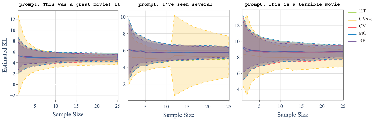
Figure 1: Comparing the bias, variance, and consistency of the estimators as the sample size increases. The $\delta_{\textsc{cv}}$ estimator with $\alpha=1$ exhibits a higher standard deviation, particularly for neutral and negative prompts, where the variance becomes extremely large. In contrast, the Rao–Blackwellized estimator, $\delta_{\textsc{rb}}$, achieves the lowest standard deviation.

4 Estimating the Gradient

KL estimation plays a crucial role in various applications, particularly in fine-tuning large language models to minimize KL divergence. One prominent example is reinforcement learning from human feedback (RLHF), where the objective function typically includes a KL regularization term to balance reward maximization with constraint adherence.

In this setting, the language model is a differentiable function of a real-valued parameter vector $\boldsymbol{\theta}$, and $\boldsymbol{\theta}$ is updated via gradient descent to maximize the KL-regularized RL objective. Therefore, an essential step in this optimization process is to compute the gradient of the KL divergence with respect to the model’s parameters, i.e.,

$$\nabla_{\boldsymbol{\theta}}\textsc{kl}(p_{\boldsymbol{\theta}}\mid\mid q)=\nabla_{\boldsymbol{\theta}}\sum_{\boldsymbol{y}\in\Sigma^{*}}p_{\boldsymbol{\theta}}(\boldsymbol{y})\log\frac{p_{\boldsymbol{\theta}}(\boldsymbol{y})}{q(\boldsymbol{y})}.$$ (18)

The standard approach to estimating the gradient is to apply the gradient operator inside the summation and then use the log-derivative trick to arrive at the following:

$$\nabla_{\boldsymbol{\theta}}\textsc{kl} =\sum_{\boldsymbol{y}\in\Sigma^{*}}\nabla_{\boldsymbol{\theta}}p_{\boldsymbol{\theta}}(\boldsymbol{y})\log\frac{p_{\boldsymbol{\theta}}(\boldsymbol{y})}{q(\boldsymbol{y})}+\nabla_{\boldsymbol{\theta}}p_{\boldsymbol{\theta}}(\boldsymbol{y})$$ (19a)

$$=\operatorname*{\mathbb{E}}\left[\left(\log\frac{p_{\boldsymbol{\theta}}(\boldsymbol{Y})}{q(\boldsymbol{Y})}+1\right)\nabla_{\boldsymbol{\theta}}\log p_{\boldsymbol{\theta}}(\boldsymbol{Y})\right].$$ (19b)

Since $\operatorname*{\mathbb{E}}[\nabla_{\boldsymbol{\theta}}\log p_{\boldsymbol{\theta}}(\boldsymbol{Y})]=0$, the gradient simplifes to

$$\nabla_{\boldsymbol{\theta}}\textsc{kl}(p_{\boldsymbol{\theta}}\mid\mid q)=\operatorname*{\mathbb{E}}\left[\log\frac{p_{\boldsymbol{\theta}}(\boldsymbol{Y})}{q(\boldsymbol{Y})}\nabla_{\boldsymbol{\theta}}\log p_{\boldsymbol{\theta}}(\boldsymbol{Y})\right].$$ (20)

Therefore, the Monte Carlo estimator of the gradient is

$$\nabla\delta_{\textsc{mc}}=\frac{1}{M}\sum_{m=1}^{M}\log\frac{p_{\boldsymbol{\theta}}(\boldsymbol{Y}^{(m)})}{q(\boldsymbol{Y}^{(m)})}\nabla_{\boldsymbol{\theta}}\log p_{\boldsymbol{\theta}}(\boldsymbol{Y}^{(m)}).$$ (21)

Next, we derive the Rao–Blackwellized Monte Carlo estimator of the gradient. However, we first restate Theorem 2.2 in (Malagutti et al., 2024), which will prove useful.

Theorem 6 (Malagutti et al. (2024); Theorem 2.2).

Let $p_{\boldsymbol{\theta}}$ and $q$ be two language models over $\Sigma$. Furthermore, let $\vec{p}$ be the prefix probability function of $p$. Furthermore, we assume that $\mathrm{H}(p,q)<\infty$. Then, the following equality holds

$$\textsc{kl}(p\mid\mid q)=\sum_{\boldsymbol{y}\in\Sigma^{*}}\vec{p}(\boldsymbol{y})\textsc{kl}\left(\vec{p}\left(\cdot\mid\boldsymbol{y}\right)\mid\mid\vec{q}\left(\cdot\mid\boldsymbol{y}\right)\right),$$ (22)

where we treat $\vec{p}(\cdot\mid\boldsymbol{y})$ and $\vec{q}\left(\cdot\mid\boldsymbol{y}\right)$ as probability distributions over $\overline{\Sigma}$.

We refer the reader to Malagutti et al. (2024) for the proof. Next, to derive the Rao–Blackwellized Monte Carlo estimator of the gradient, we take the gradient of the local KL as stated in the following theorem.

Theorem 7 (Gradient of the local KL).

Let $p_{\boldsymbol{\theta}}$ and $q$ be two language models over $\Sigma$ and $\vec{p}_{\boldsymbol{\theta}}$ the prefix probability function of $p_{\boldsymbol{\theta}}$. Furthermore, we assume that $\mathrm{H}(p_{\boldsymbol{\theta}},q)<\infty$. Then, the following equality holds

$$\begin{split}\nabla_{\boldsymbol{\theta}}\textsc{kl}(p_{\boldsymbol{\theta}}\mid\mid q)=\sum_{\boldsymbol{y}\in\Sigma^{*}}\vec{p}_{\boldsymbol{\theta}}(\boldsymbol{y})\operatorname*{\mathbb{E}}_{\overline{Y}}\Big{[}\log\frac{\vec{p}_{\boldsymbol{\theta}}(\overline{Y}\mid\boldsymbol{y})}{\vec{q}(\overline{Y}\mid\boldsymbol{y})}\\ \cdot\left(\nabla_{\boldsymbol{\theta}}\log\vec{p}_{\boldsymbol{\theta}}(\overline{Y}\mid\boldsymbol{y})+\nabla_{\boldsymbol{\theta}}\log\vec{p}_{\boldsymbol{\theta}}(\boldsymbol{y})\right)\Big{]}.\end{split}$$ (23)

Proof.

See App. F. ∎

We then construct the Monte Carlo estimator of the gradient using the above theorem, which naturally results in an unbiased Rao–Blackwellized Monte Carlo estimator of the gradient.

$$\begin{split}\nabla\delta_{\textsc{rb}}=\frac{1}{M}\sum_{m=1}^{M}\lim_{N\rightarrow\infty}\sum_{n=1}^{N}\operatorname*{\mathbb{E}}_{\overline{Y}_{n}}\Big{[}\log\frac{\vec{p}_{\boldsymbol{\theta}}(\overline{Y}_{n}\mid\overline{\boldsymbol{Y}}^{(m)}_{<n})}{\vec{q}(\overline{Y}_{n}\mid\overline{\boldsymbol{Y}}^{(m)}_{<n})}\\ \cdot\left(\nabla_{\boldsymbol{\theta}}\log\vec{p}_{\boldsymbol{\theta}}(\overline{\boldsymbol{Y}}^{(m)}_{<n})+\nabla_{\boldsymbol{\theta}}\log\vec{p}_{\boldsymbol{\theta}}(\overline{Y}_{n}\mid\overline{\boldsymbol{Y}}^{(m)}_{<n})\right)\Big{]}.\end{split}$$ (24)

The above estimator is unbiased, as it is the Monte Carlo estimator of the local KL gradient.

Theorem 8.

Let $p_{\boldsymbol{\theta}}$ and $q$ be two language models over $\Sigma$ and $\vec{p}_{\boldsymbol{\theta}}$ the prefix probability function of $p_{\boldsymbol{\theta}}$. Let $\nabla\delta_{\textsc{mc}}$ be the Monte Carlo estimator of the true gradient, denoted with $G\mathrel{\stackrel{{\scriptstyle\textnormal{def}}}{{=}}}\nabla_{\boldsymbol{\theta}}\textsc{kl}(p_{\boldsymbol{\theta}}\mid\mid q)$, as defined in Eq. 21 and $\nabla\delta_{\textsc{rb}}$ be the Rao–Blackwellized estimator of the gradient defined in Eq. 24. Assuming $\mathrm{H}(p_{\boldsymbol{\theta}},q)<\infty,\mathop{\mathrm{Var}}\left[{\normalcolor\nabla\delta_{\textsc{rb}}}\right]<\infty,\mathop{\mathrm{Var}}\left[{\normalcolor\nabla\delta_{\textsc{mc}}}\right]<\infty$, we have

$$\operatorname*{\mathbb{E}}\left[\left\lVert\nabla\delta_{\textsc{rb}}-G\right\rVert^{2}\right]\leq\operatorname*{\mathbb{E}}\left[\left\lVert\nabla\delta_{\textsc{mc}}-G\right\rVert^{2}\right].$$ (25)

Proof.

See § F.1. ∎

4.1 Off-policy Gradient

So far, we have discussed how to estimate the gradient of $\textsc{kl}(p_{\boldsymbol{\theta}}\mid\mid q)$ using samples drawn from the current policy $p_{\boldsymbol{\theta}}$. Importantly, the reason that we discussed the gradient of the estimators separately, rather than relying on the automatic differentiation, is that the samples are drawn from the $p_{\boldsymbol{\theta}}$, which depends on $\boldsymbol{\theta}$.

	$M=1$	$M=5$	$M=10$
$\delta_{\textsc{mc}}$	$6.76\pm 0.16$	$6.76\pm 0.07$	$6.76\pm 0.05$
$\delta_{\textsc{ht}}$	$6.76\pm 0.16$	$6.76\pm 0.07$	$6.76\pm 0.05$
$\delta_{\textsc{cv}},{\scriptstyle\alpha=1}$	$6.28\pm 2.54$	$6.28\pm 1.13$	$6.28\pm 0.79$
$\delta_{\textsc{cv}}$	$6.76\pm 0.16$	$6.76\pm 0.07$	$6.76\pm 0.05$
$\delta_{\textsc{rb}}$	$6.76\pm\mathbf{0.11}$	$6.76\pm\mathbf{0.05}$	$6.76\pm\mathbf{0.03}$

Table 1: Estimated value $\pm$ empirical standard deviation of different estimators. When aggregating over prompts, $\delta_{\textsc{ht}}$ and $\delta_{\textsc{cv}}$ fail to significantly reduce the variance of $\delta_{\textsc{mc}}$. Rao–Blackwellized estimator, however, achieves the lowest standard deviation.

Although on-policy reinforcement learning algorithms sample from the same policy that is being optimized, in practice and for efficiency reasons, we often collect large batches of samples in parallel with the optimization loop. As a result, these samples may be generated from a slightly outdated version of the policy, denoted $p_{\boldsymbol{\theta}_{\text{old}}}$. To compute the KL divergence using samples from $p_{\boldsymbol{\theta}_{\text{old}}}$, we first write the KL as the expectation under $p_{\boldsymbol{\theta}_{\text{old}}}$ as

$$\textsc{kl}(p_{\boldsymbol{\theta}}\mid\mid q)=\operatorname*{\mathbb{E}}_{\boldsymbol{Y}\sim p_{\boldsymbol{\theta}_{\text{old}}}}\left[\frac{p_{\boldsymbol{\theta}}(\boldsymbol{Y})}{p_{\boldsymbol{\theta}_{\text{old}}}(\boldsymbol{Y})}\log\frac{p_{\boldsymbol{\theta}}(\boldsymbol{Y})}{q(\boldsymbol{Y})}\right].$$ (26)

Therefore, the Monte Carlo estimator using samples $\boldsymbol{Y}^{(1)},\cdots,\boldsymbol{Y}^{(M)}\mathrel{\stackrel{{\scriptstyle\textnormal{i.i.d.}}}{{\sim}}}p_{\boldsymbol{\theta}_{\text{old}}}$ is

$$\delta_{\textsc{mc}}^{\text{old}}=\frac{1}{M}\sum_{m=1}^{M}\frac{p_{\boldsymbol{\theta}}(\boldsymbol{Y}^{(m)})}{p_{\boldsymbol{\theta}_{\text{old}}}(\boldsymbol{Y}^{(m)})}\log\frac{p_{\boldsymbol{\theta}}(\boldsymbol{Y}^{(m)})}{q(\boldsymbol{Y}^{(m)})}.$$ (27)

Given the unbiasedness proof of the Rao–Blackwellization in Thm. 5, we can similarly write

$$\begin{split}\textsc{kl}(p_{\boldsymbol{\theta}}\mid\mid q)=\operatorname*{\mathbb{E}}_{\boldsymbol{Y}\sim p_{\boldsymbol{\theta}_{\text{old}}}}\Bigg{[}\frac{p_{\boldsymbol{\theta}}(\boldsymbol{Y})}{p_{\boldsymbol{\theta}_{\text{old}}}(\boldsymbol{Y})}\lim_{N\rightarrow\infty}\sum_{n=1}^{N}\\ \operatorname*{\mathbb{E}}_{\overline{Y}_{n}}\left[\log\frac{\vec{p}_{\boldsymbol{\theta}}(\overline{Y}_{n}\mid\overline{\boldsymbol{Y}}_{<n})}{\vec{q}(\overline{Y}_{n}\mid\overline{\boldsymbol{Y}}_{<n})}\right]\Bigg{]}.\end{split}$$ (28)

Therefore, the Rao–Blackwellized Monte Carlo estimator using samples $\overline{\boldsymbol{Y}}^{(1)},\cdots,\overline{\boldsymbol{Y}}^{(M)}\mathrel{\stackrel{{\scriptstyle\textnormal{i.i.d.}}}{{\sim}}}p_{\boldsymbol{\theta}_{\text{old}}}$ is

$$\begin{split}\delta_{\textsc{rb}}^{\text{old}}=\frac{1}{M}\sum_{m=1}^{M}\frac{p_{\boldsymbol{\theta}}(\boldsymbol{Y}^{(m)})}{p_{\boldsymbol{\theta}_{\text{old}}}(\boldsymbol{Y}^{(m)})}\lim_{N\rightarrow\infty}\sum_{n=1}^{N}\quad\quad\\ \operatorname*{\mathbb{E}}_{\overline{Y}_{n}}\left[\log\frac{\vec{p}_{\boldsymbol{\theta}}(\overline{Y}_{n}\mid\overline{\boldsymbol{Y}}_{<n}^{(m)})}{\vec{q}(\overline{Y}_{n}\mid\overline{\boldsymbol{Y}}_{<n}^{(m)})}\right].\end{split}$$ (29)

Since $\delta_{\textsc{mc}}^{\text{old}}$ and $\delta_{\textsc{rb}}^{\text{old}}$ use samples from the old policy that does not depend on $\boldsymbol{\theta}$, we can apply automatic differentiation to compute the estimate of the KL gradient by computing the gradient of $\delta_{\textsc{mc}}^{\text{old}}$ and $\delta_{\textsc{rb}}^{\text{old}}$.

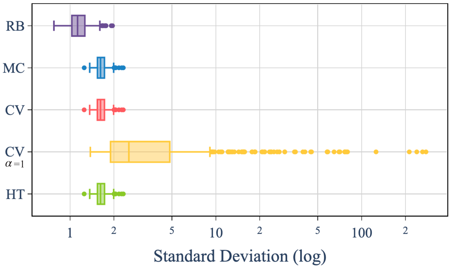
Figure 2: Standard deviation of different KL estimators across various prompts in the IMDB evaluation set, displayed on a logarithmic scale. The KL divergence is measured between a GPT-2 model before and after direct preference optimization. The $\delta_{\textsc{cv}}$ estimator with $\alpha=1$ shows considerable instability for certain prompts, whereas the Rao–Blackwellized estimator consistently yields the lowest standard deviation, indicating more stable estimates.

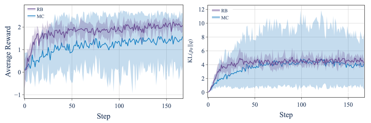
Figure 3: Comparison of the Monte Carlo (MC) and Rao–Blackwellized (RB) estimators in the RLHF fine-tuning loop. We perform RLHF with each estimator $5$ times and plot the mean and standard deviation (in shades) of the average reward values and the KL at each fine-tuning step. We observe that the MC estimator is not as stable as the RB estimator and its performance varies significantly across different runs. However, RB estimator reliably offers a good balance between achieving low KL and high reward values in all runs.

5 Experiments

We use the sentiment control task as the testbed to empirically evaluate our theoretical findings on the KL estimators. Concretely, the reference model, denoted as $q$, is the GPT-IMDB model, i.e., a GPT-2 (Radford et al., 2019) model fine-tuned on imdb corpus (Maas et al., 2011). The goal of the task is to fine-tune this language model such that the samples from it are movie reviews with a positive sentiment. The fine-tuned language model is denoted with $p_{\boldsymbol{\theta}}$. In the following experiments, we estimate the KL divergence between $p_{\boldsymbol{\theta}}$ and $q$.

5.1 Understanding the KL Estimators

In this experiment, we empirically evaluate the bias, variance, and consistency of various KL estimators. To obtain $p_{\boldsymbol{\theta}}$, we fine-tune $q$ with direct preference optimization (DPO; Rafailov et al., 2023) on a sample of 5,000 data points from the IMDB training set. To create the preference data required for DPO training, following Rafailov et al. (2023), we sample $4$ responses for each prompt and create $6$ pairs per prompt. To determine the preferred response in each pair, we employ a binary sentiment classifier, selecting the response with the higher probability of positive sentiment. Upon successful fine-tuning, $p_{\boldsymbol{\theta}}$ should assign a higher probability mass to movie reviews with positive sentiment while maintaining a low KL divergence with $q$. We then evaluate this KL divergence using our estimators to assess their reliability in measuring distributional shifts induced by fine-tuning.

We sample 512 examples from the evaluation set of the IMDB corpus. For each example, we randomly select a prefix length between 2 and 8 tokens and use it as the prompt. Then, for each prompt, we generate 4000 samples from the DPO fine-tuned model, $p_{\boldsymbol{\theta}}$. Using these samples, we compute the MC, CV, and RB estimators and empirically estimate their standard deviation. We further implement and compare the Horvitz–Thompson estimator; we refer the reader to App. A for a detailed discussion. We compute the Monte Carlo estimator with control variate, $\delta_{\textsc{cv}}$, twice: once using the optimal $\alpha$ value derived from 1000 samples and once with $\alpha=1$, matching the setup of Schulman (2020).

In Tab. 1, we report the expected KL estimate along with the empirical standard deviation of different estimators evaluated at sample sizes $M=1,5,10$. To obtain these estimates, we compute each estimator using $M$ samples, repeating the process $4000/M$ times to estimate both the expected value and the standard deviation of the estimates. Our findings confirm that all estimators except one ($\delta_{\textsc{cv}},\alpha=1$), are unbiased and report an expected KL divergence of $6.76$. We also observe that the CV estimators fail to significantly reduce the variance of the standard Monte Carlo estimator. Importantly, Rao–Blackwellized Monte Carlo estimator achieves the lowest standard deviation and offers a more robust estimate compared to the MC estimator. Interestingly, when setting $\alpha=1$, the control variate Monte Carlo estimator exhibits both noticeable bias and high variance. To investigate this further, we next examine KL divergence estimates at the level of individual prompts.

In Fig. 1, we visualize the KL estimates for three different prompts: (left) a positive prompt, (middle) a neutral prompt, and (right) a negative adversarial prompt. The traces represent the average estimates from all the repetitions, while the shaded regions indicate the standard deviation. Except $\delta_{\textsc{cv}},\alpha=1$, all other estimators are unbiased and consistent. We observe that the $\delta_{\textsc{cv}}$ estimator exhibits a noticeable bias and high standard deviation when $\alpha=1$, i.e., when it is not set to its optimal value. The bias arises from numerical instability during the computation of $g(\boldsymbol{Y})=\frac{q(\boldsymbol{Y})}{p(\boldsymbol{Y})}-1$. The high variance is due to large values of $\mathop{\mathrm{Var}}\left[{\normalcolor g(\boldsymbol{Y})}\right]$. Specifically, for certain prompts, $\mathop{\mathrm{Var}}\left[{\normalcolor g(\boldsymbol{Y})}\right]$ can be unbounded. As the sample size increases, the chance of sampling from the tail of $p_{\boldsymbol{\theta}}$ also increases. These tail samples often correspond to negative movie reviews that had a high probability under the language model prior to fine-tuning, i.e., $q$, leading to extremely large values of $g(\boldsymbol{Y})$ and, consequently, a high standard deviation. This effect indeed depends on the prompt and is particularly pronounced for neutral and adversarial prompts.

Since the robustness of the estimators depends on the choice of the prompt, we further analyze their estimated standard deviations across all prompts. Fig. 2 presents a box plot of standard deviations (log scale) for each estimator. The $\delta_{\textsc{cv}}$ estimator with $\alpha=1$ shows significant instability for certain prompts, with numerous outliers indicating high variance. In contrast, the $\delta_{\textsc{mc}}$ and the standard $\delta_{\textsc{cv}}$ estimators exhibit comparable standard deviations. Notably, the Rao–Blackwellized estimator consistently achieves the lowest standard deviation, suggesting it provides the most stable estimates.

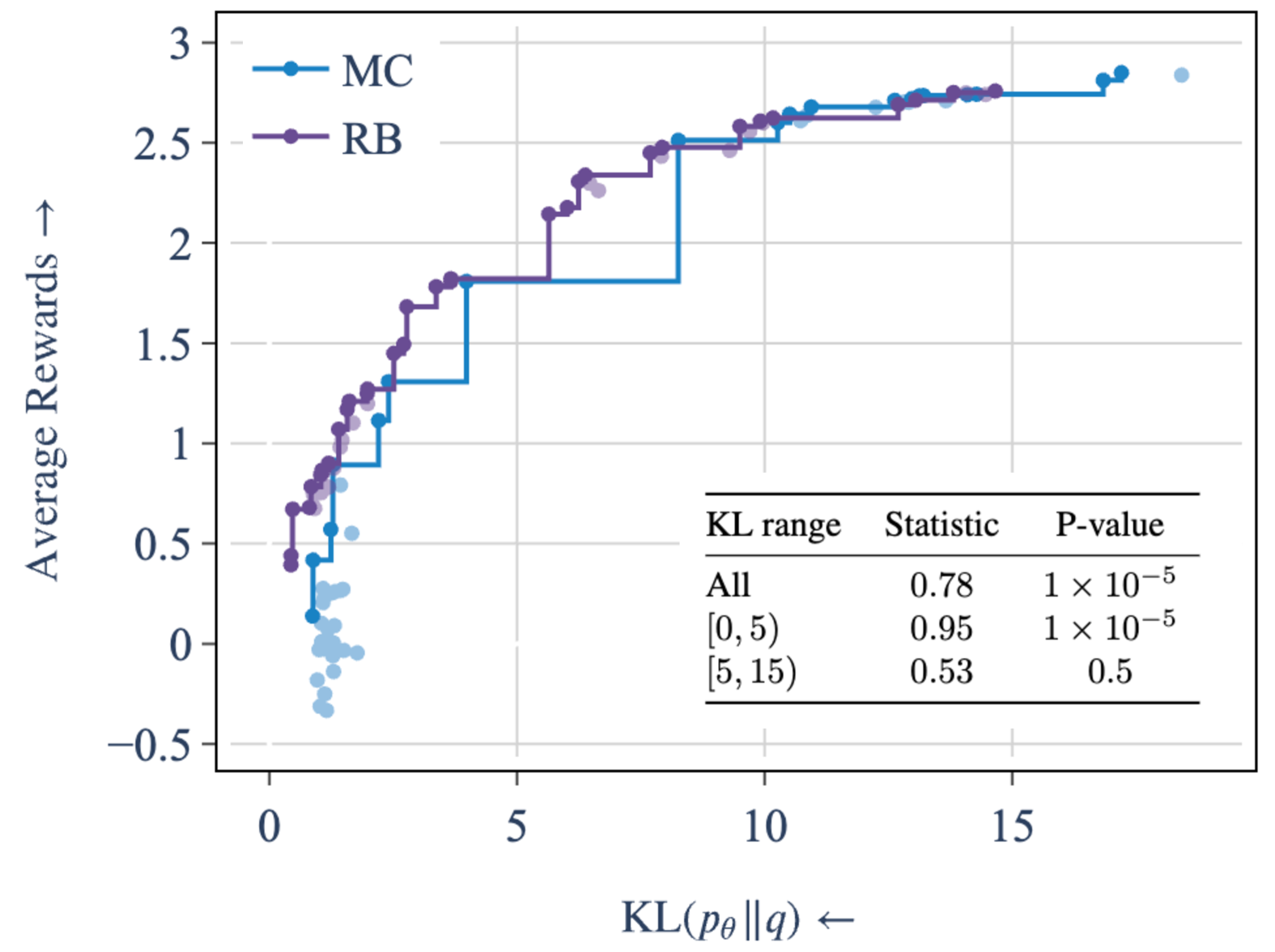
Figure 4: In comparison to models that are trained under the MC estimator, models that are trained with the RB estimator appear on the overall Pareto front $76\%$ of the time. We visualize the Pareto front for each estimator and show the fine-tuning runs that do not end up on the Pareto front with a lower opacity. RB estimator is more effective compared to the MC estimator in constraining the model to maintain a low KL while achieving reasonable rewards.

5.2 KL Estimation and RLHF Training Dynamics

A key application of KL estimation is in the RLHF training loop. From the previous experiment, we observed that the Rao–Blackwellized estimator significantly reduces the standard deviation of the Monte Carlo estimator. Therefore, it is natural to ask how this affects RLHF performance when this estimator is used in the training loop. The RLHF objective consists of two terms: (i) the expected rewards for samples generated by the language model $p_{\boldsymbol{\theta}}$, which in this case is the samples’ score under a sentiment classifier, and (ii) the negative KL divergence between the fine-tuned model $p_{\boldsymbol{\theta}}$ and the reference model $q$, which represents the language model before fine-tuning.

We compare the Monte Carlo and Rao–Blackwellized estimators for computing the gradient of the KL divergence term in the RLHF training loop. We use the RL algorithm proposed by Ahmadian et al. (2024), which is an improved version of the reinforce algorithm (Williams, 1992). We track two metrics throughout fine-tuning: (i) the average reward associated with samples drawn from $p_{\boldsymbol{\theta}}$, and (ii) the KL divergence between $p_{\boldsymbol{\theta}}$ and $q$. The results are visualized in Fig. 3. The purple trace represents the training run where the $\delta_{\textsc{rb}}$ is used in the optimization loop to estimate the gradient of the KL divergence, while the blue trace represents the run using $\delta_{\textsc{mc}}$. The x-axis denotes the fine-tuning step, with the left plot showing the evolution of the average reward and the right plot displaying the KL divergence between $p_{\boldsymbol{\theta}}$ and $q$ over the course of fine-tuning. We repeat each experiment $5$ times and report the mean and standard deviation of each metric. Notably, the KL values in the right plot are estimated using the Rao–Blackwellized estimator. However, we observe the same overall trend when using the Monte Carlo estimator for evaluation.

As illustrated in Fig. 3, the performance of the models trained using the MC estimator varies significantly across the $5$ experiments, resulting in a large standard deviation in both average rewards and the KL divergence. However, Rao–Blackwellized estimator consistantly achieves high rewards and reasonable KL values across all runs. This observation suggests that reducing the variance of the KL estimator makes the RLHF more reliable.

Finally, we vary the KL coefficient, $\beta$, in $[0.01,0.1]$ range and fine-tune $18$ models with each estimator. For each estimator, we plot the Pareto frontier of average rewards versus KL divergence in Fig. 4, displaying models that do not appear on the Pareto front with reduced opacity. Overall, we find that fine-tuning with the RB estimator is more effective at achieving high rewards while maintaining a low KL divergence from the reference model. To quantify this effect, we compute the fraction of RB fine-tuned models that appear on the overall Pareto front—i.e., the frontier obtained when considering all models fine-tuned with either estimator. We then conduct a permutation test and report the results in Fig. 4. We find that $76\%$ of the points on the overall Pareto front come from RB fine-tuned models. Restricting to models with KL values below $5$, this fraction rises to $95\%$, with both results being statistically significant.

6 Conclusion

In this paper, we study the problem of estimating the KL divergence between language models. We provide a comprehensive formal analysis of various KL estimators, with a focus on their bias and variance. We introduce a Rao–Blackwellized Monte Carlo estimator, which is provably unbiased and has variance at most equal to that of the standard Monte Carlo estimator. This estimator applies the well-known Rao–Blackwellization technique to reduce the variance of the standard Monte Carlo method. Our empirical results show that the Rao–Blackwellized estimator significantly reduces the variance compared to the Monte Carlo estimator, while other estimators fail to achieve meaningful variance reduction or, in some cases, suffer from unbounded variance. Additionally, we find that using our proposed Rao–Blackwellized estimator makes RLHF more stable and produces models that more frequently lie on the Pareto frontier of reward versus KL, compared to models fine-tuned with the Monte Carlo estimator.

Impact Statement

In this paper, we investigate the fundamental problem of estimating KL divergence between language models. One key application of KL estimation is in RLHF, which aims to enhance fluency while aligning language models with user preferences. However, RLHF can also be misused by bad actors to optimize models for generating misleading, biased, or harmful content. While our work provides a deeper understanding of KL estimation techniques, it is purely foundational research and does not introduce new risks or directly contribute to harmful applications.

Appendix A Horvitz–Thompson Estimation

When estimating the KL divergence between two language models $p$ and $q$, we have access not only to samples from $p$ but also to the probability assigned by $p$ to any string $\boldsymbol{y}$. This enables the use of a more informed estimator, which leverages these probabilities during its construction. Notably, this estimator is a specific instance of the Horvitz–Thompson (HT) estimator (Horvitz and Thompson, 1952), defined as []

$$\delta_{\textsc{ht}}=\sum_{\boldsymbol{y}\in S}\frac{p(\boldsymbol{y})}{\pi_{S}(\boldsymbol{y})}\log\frac{p(\boldsymbol{y})}{q(\boldsymbol{y})}=\sum_{\boldsymbol{y}\in S}\frac{p(\boldsymbol{y})}{\pi_{S}(\boldsymbol{y})}f(\boldsymbol{y}),$$ (30)

where $S$ is the random variable representing the set of all sampled strings. Any sampling design can be specified to generate the elements of $S$. The inclusion probability, denoted by $\pi_{S}(\boldsymbol{y})$, is the probability that a particular string $\boldsymbol{y}$ is included in $S$, or equivalently, $\operatorname*{\mathbb{E}}\left[\mathbbm{1}\{\boldsymbol{y}\in S\}\right]$.

Proposition 9.

$\delta_{\textsc{ht}}$ is an unbiased estimator of the KL divergence, i.e., $\operatorname*{\mathbb{E}}\big{[}\delta_{\textsc{ht}}\big{]}-\textsc{kl}(p\mid\mid q)=0$.

Proof.

The bias of the estimator is as follows:

$$\operatorname*{\mathbb{E}}_{S}\Big{[}\delta_{\textsc{ht}}\Big{]}-\textsc{kl}(p\mid\mid q) =\operatorname*{\mathbb{E}}_{S}\Big{[}\sum_{\boldsymbol{y}\in S}\frac{p(\boldsymbol{y})}{\pi_{S}(\boldsymbol{y})}\log\frac{p(\boldsymbol{y})}{q(\boldsymbol{y})}\Big{]}-\textsc{kl}(p\mid\mid q) \delta_{\textsc{ht}}$$ (definition of ) (31a)

$$=\operatorname*{\mathbb{E}}_{S}\Big{[}\sum_{\boldsymbol{y}\in\Sigma^{*}}\frac{p(\boldsymbol{y})}{\pi_{S}(\boldsymbol{y})}\log\frac{p(\boldsymbol{y})}{q(\boldsymbol{y})}\,\cdot\,\mathbbm{1}\{\boldsymbol{y}\in S\}\Big{]}-\textsc{kl}(p\mid\mid q)$$ (31b)

$$=\sum_{\boldsymbol{y}\in\Sigma^{*}}\frac{p(\boldsymbol{y})}{\pi_{S}(\boldsymbol{y})}\log\frac{p(\boldsymbol{y})}{q(\boldsymbol{y})}\,\cdot\,\operatorname*{\mathbb{E}}_{S}\Big{[}\mathbbm{1}\{\boldsymbol{y}\in S\}\Big{]}-\textsc{kl}(p\mid\mid q)$$ (linearity of expectation) (31c)

$$=\sum_{\boldsymbol{y}\in\Sigma^{*}}\frac{p(\boldsymbol{y})}{\cancel{\pi_{S}(\boldsymbol{y})}}\log\frac{p(\boldsymbol{y})}{q(\boldsymbol{y})}\,\cdot\,\cancel{\pi_{S}(\boldsymbol{y})}-\textsc{kl}(p\mid\mid q) \pi_{S}(\boldsymbol{y})$$ (definition of ) (31d)

$$=0.$$ (31e)

∎

Similar to the MC estimator, the HT estimator does not necessarily return a non-negative estimate of the KL. In principle, however, we should prefer Eq. 30 to Eq. 6a because it exploits more information—namely, the knowledge of $p$. Whether the HT estimator yields lower variance than the MC estimator depends on the sampling design used to construct $S$. In our experiments in App. G, we used the sampling-with-replacement design, where $\pi_{S}(\boldsymbol{y})=1-\left(1-p(\boldsymbol{y})\right)^{M}$. Compared to the MC estimator, we observed no significant reduction in variance in our experiments.

Appendix B Proof of Prop. 1

See 1

Proof.

First, we remind the reader that the control variate Monte Carlo estimator was defined in Eq. 8 as See 4

Note that $\{\boldsymbol{Y}^{(m)}\}_{m=1}^{M}\mathrel{\stackrel{{\scriptstyle\textnormal{i.i.d.}}}{{\sim}}}p$. Next, we compute the bias and variance of this estimator as follows:

$$\operatorname*{\mathbb{E}}\left[\delta_{\textsc{cv}}\right]-\textsc{kl}=\frac{1}{M}\sum_{m=1}^{M}\operatorname*{\mathbb{E}}\left[f(\boldsymbol{Y}^{(m)})\right]+\alpha\underbrace{(\operatorname*{\mathbb{E}}\left[g(\boldsymbol{Y}^{(m)})\right]-G)}_{=0}-\textsc{kl}=\operatorname*{\mathbb{E}}\left[f(\boldsymbol{Y})\right]-\textsc{kl}=0$$ (32a)

$$\mathop{\mathrm{Var}}\left[{\normalcolor\delta_{\textsc{cv}}}\right]=\frac{1}{M}\mathop{\mathrm{Var}}\left[{\normalcolor f+\alpha(g-G)}\right]=\frac{1}{M}\mathop{\mathrm{Var}}\left[{\normalcolor f}\right]+\frac{\alpha^{2}}{M}\mathop{\mathrm{Var}}\left[{\normalcolor g}\right]+\frac{2\alpha}{M}\mathop{\mathrm{Cov}}\left[{\normalcolor f,g}\right].$$ (32b)

∎

Appendix C Proof of Prop. 2

See 2

Proof.

$$\mathop{\mathrm{Cov}}\left[{\normalcolor f,g}\right] =\operatorname*{\mathbb{E}}\left[\left(\log\frac{p(\boldsymbol{Y})}{q(\boldsymbol{Y})}-\operatorname*{\mathbb{E}}\left[\log\frac{p(\boldsymbol{Y})}{q(\boldsymbol{Y})}\right]\right)\left(\frac{q(\boldsymbol{Y})}{p(\boldsymbol{Y})}-\underbrace{\operatorname*{\mathbb{E}}\left[\frac{q(\boldsymbol{Y})}{p(\boldsymbol{Y})}\right]}_{=1}\right)\right]$$ (33a)

$$=\operatorname*{\mathbb{E}}\left[\frac{q(\boldsymbol{Y})}{p(\boldsymbol{Y})}\log\frac{p(\boldsymbol{Y})}{q(\boldsymbol{Y})}-\cancel{\log\frac{p(\boldsymbol{Y})}{q(\boldsymbol{Y})}}-\operatorname*{\mathbb{E}}\left[\log\frac{p(\boldsymbol{Y})}{q(\boldsymbol{Y})}\right]\frac{q(\boldsymbol{Y})}{p(\boldsymbol{Y})}+\cancel{\operatorname*{\mathbb{E}}\left[\log\frac{p(\boldsymbol{Y})}{q(\boldsymbol{Y})}\right]}\right]$$ (33b)

$$=\operatorname*{\mathbb{E}}\left[\frac{q(\boldsymbol{Y})}{p(\boldsymbol{Y})}\log\frac{p(\boldsymbol{Y})}{q(\boldsymbol{Y})}\right]-\operatorname*{\mathbb{E}}\left[\log\frac{p(\boldsymbol{Y})}{q(\boldsymbol{Y})}\right]\underbrace{\operatorname*{\mathbb{E}}\left[\log\frac{q(\boldsymbol{Y})}{p(\boldsymbol{Y})}\right]}_{=1}$$ (33c)

$$=\operatorname*{\mathbb{E}}\left[-\frac{q(\boldsymbol{Y})}{p(\boldsymbol{Y})}\log\frac{q(\boldsymbol{Y})}{p(\boldsymbol{Y})}\right]-\operatorname*{\mathbb{E}}\left[\log\frac{p(\boldsymbol{Y})}{q(\boldsymbol{Y})}\right]$$ (33d)

$$=-\textsc{kl}(q\mid\mid p)-\textsc{kl}(p\mid\mid q).$$ (33e)

∎

Appendix D Connection to Bregman Divergence

Bregman divergence (Bregman, 1967) is a measure of the difference between a convex function and its tangent plane. Let $F:\Omega\rightarrow\mathbb{R}$ be a strictly convex function, where $\Omega$ is a convex set. Bregman divergence associated with $F$ is defined as

$$D_{F}(p,q)=F(p)-F(q)-\langle\nabla_{\boldsymbol{\theta}}F(q),p-q\rangle.$$ (34)

Proposition 10.

Let $F(p)=-\mathrm{H}(p)$, defined as $\mathrm{H}(p)=\sum_{\boldsymbol{y}\in\Sigma^{*}}-p(\boldsymbol{y})\log p(\boldsymbol{y})$. Then, the Bregman divergence $D_{F}(p,q)=\textsc{kl}(p\mid\mid q)$.

Proof.

$$D_{F}(p,q) \mathrel{\stackrel{{\scriptstyle\textnormal{def}}}{{=}}}\sum_{\boldsymbol{y}\in\Sigma^{*}}p(\boldsymbol{y})\log p(\boldsymbol{y})-q(\boldsymbol{y})\log q(\boldsymbol{y})-\big{(}\log q(\boldsymbol{y})+1\big{)}\big{(}p(\boldsymbol{y})-q(\boldsymbol{y})\big{)}$$ (35a)

$$=\sum_{\boldsymbol{y}\in\Sigma^{*}}p(\boldsymbol{y})\log p(\boldsymbol{y})-q(\boldsymbol{y})\log q(\boldsymbol{y})+q(\boldsymbol{y})\log q(\boldsymbol{y})-p(\boldsymbol{y})\log q(\boldsymbol{y})-p(\boldsymbol{y})+q(\boldsymbol{y})$$ (35b)

$$=\sum_{\boldsymbol{y}\in\Sigma^{*}}p(\boldsymbol{y})\Big{(}\log\frac{p(\boldsymbol{y})}{q(\boldsymbol{y})}+\frac{q(\boldsymbol{y})}{p(\boldsymbol{y})}-1\Big{)}$$ (35c)

$$=\sum_{\boldsymbol{y}\in\Sigma^{*}}p(\boldsymbol{y})\log\frac{p(\boldsymbol{y})}{q(\boldsymbol{y})}+\cancelto{0}{\sum_{\boldsymbol{y}\in\Sigma^{*}}q(\boldsymbol{y})-p(\boldsymbol{y})}$$ (35d)

$$=\textsc{kl}(p\mid\mid q).$$ (35e)

∎

We can rewrite Eq. 35c as

$$D_{F}(p,q)=\operatorname*{\mathbb{E}}\left[\log\frac{p(\boldsymbol{Y})}{q(\boldsymbol{Y})}+\frac{q(\boldsymbol{Y})}{p(\boldsymbol{Y})}-1\right],$$ (36)

where $\boldsymbol{Y}\sim p$. Note that the estimator $\delta_{\textsc{cv}}$ Eq. 11 (with $\alpha=1$) is nothing but an MC estimator for Eq. 36.

Appendix E Rao–Blackwellized Estimator

E.1 Proof of Lemma 3

See 3

Proof.

$$\delta_{\textsc{mc}} =\frac{1}{M}\sum_{m=1}^{M}\log\frac{p(\boldsymbol{Y}^{(m)})}{q(\boldsymbol{Y}^{(m)})}$$ (37a)

$$=\frac{1}{M}\sum_{m=1}^{M}\log\frac{\vec{p}(\textsc{eos}\mid\boldsymbol{Y}^{(m)})}{\vec{q}(\textsc{eos}\mid\boldsymbol{Y}^{(m)})}\prod_{n=1}^{|\boldsymbol{Y}^{(m)}|}\log\frac{\vec{p}(Y^{(m)}_{n}\mid\boldsymbol{Y}^{(m)}_{<n})}{\vec{q}(Y^{(m)}_{n}\mid\boldsymbol{Y}^{(m)}_{<n})}$$ (37b)

$$=\frac{1}{M}\sum_{m=1}^{M}\log\prod_{n=1}^{\infty}\frac{\vec{p}(\overline{Y}^{(m)}_{n}\mid\overline{\boldsymbol{Y}}^{(m)}_{<n})}{\vec{q}(\overline{Y}^{(m)}_{n}\mid\overline{\boldsymbol{Y}}^{(m)}_{<n})}$$ (37c)

$$=\frac{1}{M}\sum_{m=1}^{M}\log\lim_{N\rightarrow\infty}\prod_{n=1}^{N}\frac{\vec{p}(\overline{Y}^{(m)}_{n}\mid\overline{\boldsymbol{Y}}^{(m)}_{<n})}{\vec{q}(\overline{Y}^{(m)}_{n}\mid\overline{\boldsymbol{Y}}^{(m)}_{<n})}$$ (37d)

$$=\lim_{N\rightarrow\infty}\frac{1}{M}\sum_{m=1}^{M}\log\prod_{n=1}^{N}\frac{\vec{p}(\overline{Y}^{(m)}_{n}\mid\overline{\boldsymbol{Y}}^{(m)}_{<n})}{\vec{q}(\overline{Y}^{(m)}_{n}\mid\overline{\boldsymbol{Y}}^{(m)}_{<n})}$$ (37e)

$$=\lim_{N\rightarrow\infty}\frac{1}{M}\sum_{m=1}^{M}\log\frac{\vec{p}(\overline{\boldsymbol{Y}}^{(m)}_{\leq N})}{\vec{q}(\overline{\boldsymbol{Y}}^{(m)}_{\leq N})}$$ (37f)

$$=\lim_{N\rightarrow\infty}\delta_{\textsc{mc}}^{N}.$$ (37g)

Note that going from Eq. 37b to Eq. 37c, we lift the language model to a language process using the construction given in § E.2. ∎

E.2 Proof of Lemma 4

See 4

Proof.

In the proof below, we consider the case where $M=1$. The proof easily generalizes to $M>1$ using the i.i.d. assumption. Additionally, we write $\delta_{\textsc{rb}}^{N}(\overline{\boldsymbol{Y}})$, rather than suppressing the argument to the estimator as we do in the main text. We begin by proving the unbiasedness property of the estimator.

$$\operatorname*{\mathbb{E}}\big{[}\delta_{\textsc{rb}}^{N}\big{]}-\operatorname*{\mathbb{E}}[\delta_{\textsc{mc}}^{N}] =\operatorname*{\mathbb{E}}_{\overline{\boldsymbol{Y}}^{\prime}}\Big{[}\sum_{n=1}^{N}\operatorname*{\mathbb{E}}_{\overline{\boldsymbol{Y}}}\big{[}\delta_{\textsc{mc}}^{n}(\overline{\boldsymbol{Y}})\mid\overline{\boldsymbol{Y}}_{<n}=\overline{\boldsymbol{Y}}^{\prime}_{<n}\big{]}\Big{]}-\operatorname*{\mathbb{E}}[\delta_{\textsc{mc}}^{N}] \delta_{\textsc{rb}}^{N}$$ (definition of ) (38a)

$$=\sum_{n=1}^{N}\operatorname*{\mathbb{E}}_{\overline{\boldsymbol{Y}}^{\prime}}\Big{[}\operatorname*{\mathbb{E}}_{\overline{\boldsymbol{Y}}}\big{[}\delta_{\textsc{mc}}^{n}(\overline{\boldsymbol{Y}})\mid\overline{\boldsymbol{Y}}_{<n}=\overline{\boldsymbol{Y}}^{\prime}_{<n}\big{]}\Big{]}-\operatorname*{\mathbb{E}}[\delta_{\textsc{mc}}^{N}]$$ (linearity of expectation) (38b)

$$=\sum_{n=1}^{N}\operatorname*{\mathbb{E}}_{\overline{\boldsymbol{Y}}}\left[\delta_{\textsc{mc}}^{n}(\overline{\boldsymbol{Y}})\right]-\operatorname*{\mathbb{E}}[\delta_{\textsc{mc}}^{N}]$$ (law of total expectation) (38c)

$$=\operatorname*{\mathbb{E}}_{\overline{\boldsymbol{Y}}}\left[\sum_{n=1}^{N}\delta_{\textsc{mc}}^{n}(\overline{\boldsymbol{Y}})\right]-\operatorname*{\mathbb{E}}[\delta_{\textsc{mc}}^{N}]$$ (linearity of expectation) (38d)

$$=0. \delta_{\textsc{mc}}^{N}=\sum_{n=1}^{N}\delta_{\textsc{mc}}^{n}$$ () (38e)

Next, we prove the variance reduction property:

$$\mathop{\mathrm{Var}}\left[{\normalcolor\delta_{\textsc{rb}}^{N}}\right] =\operatorname*{\mathbb{E}}_{\overline{\boldsymbol{Y}}^{\prime}}\left[\left(\sum_{n=1}^{N}\operatorname*{\mathbb{E}}_{\overline{\boldsymbol{Y}}}\left[\delta_{\textsc{mc}}^{n}(\overline{\boldsymbol{Y}})\,\middle|\,\overline{\boldsymbol{Y}}_{<n}=\overline{\boldsymbol{Y}}^{\prime}_{<n}\right]-\operatorname*{\mathbb{E}}[\delta_{\textsc{rb}}^{N}]\right)^{2}\right]$$ (39a)

$$\begin{subarray}{c}\text{{\color[rgb]{.5,.5,.5}(defintion of $\delta_{\textsc{rb}}^{N}$)}}\end{subarray}$$

$$=\operatorname*{\mathbb{E}}_{\overline{\boldsymbol{Y}}^{\prime}}\left[\left(\sum_{n=1}^{N}\operatorname*{\mathbb{E}}_{\overline{\boldsymbol{Y}}^{n}}\left[\delta_{\textsc{mc}}^{n}(\overline{\boldsymbol{Y}}^{n})\,\middle|\,\overline{\boldsymbol{Y}}^{n}_{<n}=\overline{\boldsymbol{Y}}^{\prime}_{<n}\right]-\operatorname*{\mathbb{E}}[\delta_{\textsc{rb}}^{N}]\right)^{2}\right]$$ (39b)

$$\begin{subarray}{c}\text{{\color[rgb]{.5,.5,.5}($\{\overline{\boldsymbol{Y}}^{n}\}_{n=1}^{N}$ are i.i.d. )}}\end{subarray}$$

$$=\operatorname*{\mathbb{E}}_{\overline{\boldsymbol{Y}}^{\prime}}\left[\left(\sum_{n=1}^{N}\operatorname*{\mathbb{E}}_{\overline{\boldsymbol{Y}}^{n}}\left[\delta_{\textsc{mc}}^{n}(\overline{\boldsymbol{Y}}^{n})-\operatorname*{\mathbb{E}}[\delta_{\textsc{rb}}^{N}]\,\middle|\,\overline{\boldsymbol{Y}}^{n}_{<n}=\overline{\boldsymbol{Y}}^{\prime}_{<n}\right]\right)^{2}\right]$$ (39c)

$$\begin{subarray}{c}\text{{\color[rgb]{.5,.5,.5}(linearity of expectation)}}\end{subarray}$$

$$=\operatorname*{\mathbb{E}}_{\overline{\boldsymbol{Y}}^{\prime}}\left[\left(\operatorname*{\mathbb{E}}_{\overline{\boldsymbol{Y}}^{1}}\left[\cdots\operatorname*{\mathbb{E}}_{\overline{\boldsymbol{Y}}^{N}}\left[\sum_{n=1}^{N}\delta_{\textsc{mc}}^{n}(\overline{\boldsymbol{Y}}^{n})-\operatorname*{\mathbb{E}}[\delta_{\textsc{rb}}^{N}]\,\middle|\,\overline{\boldsymbol{Y}}^{N}_{<N}=\overline{\boldsymbol{Y}}^{\prime}_{<N}\right]\cdots\,\middle|\,\overline{\boldsymbol{Y}}^{1}_{<1}=\overline{\boldsymbol{Y}}^{\prime}_{<1}\right]\right)^{2}\right]$$ (39d)

$$\begin{subarray}{c}\text{{\color[rgb]{.5,.5,.5}(linearity of expectation)}}\end{subarray}$$

$$\leq\operatorname*{\mathbb{E}}_{\overline{\boldsymbol{Y}}^{\prime}}\left[\operatorname*{\mathbb{E}}_{\overline{\boldsymbol{Y}}^{1}}\left[\cdots\operatorname*{\mathbb{E}}_{\overline{\boldsymbol{Y}}^{N}}\left[\left(\sum_{n=1}^{N}\delta_{\textsc{mc}}^{n}(\overline{\boldsymbol{Y}}^{n})-\operatorname*{\mathbb{E}}[\delta_{\textsc{rb}}^{N}]\right)^{2}\,\middle|\,\overline{\boldsymbol{Y}}^{N}_{<N}=\overline{\boldsymbol{Y}}^{\prime}_{<N}\right]\cdots\,\middle|\,\overline{\boldsymbol{Y}}^{1}_{<1}=\overline{\boldsymbol{Y}}^{\prime}_{<1}\right]\right]$$ (39e)

$$\begin{subarray}{c}\text{{\color[rgb]{.5,.5,.5}(Jensen's inequality)}}\end{subarray}$$

$$=\operatorname*{\mathbb{E}}_{\overline{\boldsymbol{Y}}^{1}}\left[\cdots\operatorname*{\mathbb{E}}_{\overline{\boldsymbol{Y}}^{N}}\left[\left(\sum_{n=1}^{N}\delta_{\textsc{mc}}^{n}(\overline{\boldsymbol{Y}}^{n})-\operatorname*{\mathbb{E}}[\delta_{\textsc{rb}}^{N}]\right)^{2}\right]\right]$$ (39f)

$$\begin{subarray}{c}\text{{\color[rgb]{.5,.5,.5}(law of total expectation)}}\end{subarray}$$

$$=\operatorname*{\mathbb{E}}_{\overline{\boldsymbol{Y}}}\left[\left(\sum_{n=1}^{N}\delta_{\textsc{mc}}^{n}(\overline{\boldsymbol{Y}})-\operatorname*{\mathbb{E}}[\delta_{\textsc{rb}}^{N}]\right)^{2}\right]$$ (39g)

$$\begin{subarray}{c}\text{{\color[rgb]{.5,.5,.5}($\{\overline{\boldsymbol{Y}}^{n}\}_{n=1}^{N}$ are i.i.d. )}}\end{subarray}$$

$$=\operatorname*{\mathbb{E}}_{\overline{\boldsymbol{Y}}}\left[\left(\delta_{\textsc{mc}}^{N}(\overline{\boldsymbol{Y}})-\operatorname*{\mathbb{E}}[\delta_{\textsc{mc}}^{N}]\right)^{2}\right]$$ (39h)

$$\begin{subarray}{c}\text{{\color[rgb]{.5,.5,.5}($\delta_{\textsc{mc}}^{N}(\boldsymbol{Y})=\sum_{n=1}^{N}\delta_{\textsc{mc}}^{n}(\boldsymbol{Y}_{\leq n})$)}}\end{subarray}$$

$$=\mathop{\mathrm{Var}}\left[{\normalcolor\delta_{\textsc{mc}}^{N}}\right].$$ (39i)

$$\begin{subarray}{c}\text{{\color[rgb]{.5,.5,.5}(definition of variance)}}\end{subarray}$$

∎

E.3 Proof of Thm. 5

See 5

Proof.

First, in the following lemma, we prove that $\delta_{\textsc{mc}}$ can be decomposed into steps for the unbounded case as well. In the rest of the proof, we consider the special case of $M=1$. The proof easily generalizes to $M>1$ using the i.i.d. assumption. Additionally, we write $\delta_{\textsc{rb}}(\overline{\boldsymbol{Y}})$, rather than suppressing the argument to the estimator as we do in the main text. We begin with proving the unbiasedness of the estimator.

$$\operatorname*{\mathbb{E}}\big{[}\delta_{\textsc{rb}}(\overline{\boldsymbol{Y}})\big{]}-\textsc{kl}(p\mid\mid q) =\operatorname*{\mathbb{E}}_{\overline{\boldsymbol{Y}}^{\prime}}\Big{[}\lim_{N\rightarrow\infty}\sum_{n=1}^{N}\operatorname*{\mathbb{E}}_{\overline{\boldsymbol{Y}}}\big{[}\delta_{\textsc{mc}}^{n}(\overline{\boldsymbol{Y}})\mid\overline{\boldsymbol{Y}}_{<n}=\overline{\boldsymbol{Y}}^{\prime}_{<n}\big{]}\Big{]}-\textsc{kl}(p\mid\mid q)$$ (40a)

$$=\lim_{N\rightarrow\infty}\sum_{n=1}^{N}\operatorname*{\mathbb{E}}_{\overline{\boldsymbol{Y}}^{\prime}}\Big{[}\operatorname*{\mathbb{E}}_{\overline{\boldsymbol{Y}}}\big{[}\delta_{\textsc{mc}}^{n}(\overline{\boldsymbol{Y}})\mid\overline{\boldsymbol{Y}}_{<n}=\overline{\boldsymbol{Y}}^{\prime}_{<n}\big{]}\Big{]}-\textsc{kl}(p\mid\mid q)$$ (40b)

$$\begin{subarray}{c}\text{{\color[rgb]{.5,.5,.5}(Tonelli's Theorem)}}\end{subarray}$$

$$=\lim_{N\rightarrow\infty}\sum_{n=1}^{N}\operatorname*{\mathbb{E}}_{\overline{\boldsymbol{Y}}}\left[\delta_{\textsc{mc}}^{n}(\overline{\boldsymbol{Y}})\right]-\textsc{kl}(p\mid\mid q)$$ (40c)

$$\begin{subarray}{c}\text{{\color[rgb]{.5,.5,.5}(\lx@cref{creftypecap~refnum}{lemma:rb})}}\end{subarray}$$

$$=\operatorname*{\mathbb{E}}_{\overline{\boldsymbol{Y}}}\left[\lim_{N\rightarrow\infty}\sum_{n=1}^{N}\delta_{\textsc{mc}}^{n}(\overline{\boldsymbol{Y}})\right]-\textsc{kl}(p\mid\mid q)$$ (40d)

$$\begin{subarray}{c}\text{{\color[rgb]{.5,.5,.5}(Fubini's Theorem,$\operatorname*{\mathbb{E}}\left[\sum_{n=1}^{\infty}|\delta_{\textsc{mc}}^{n}(\overline{\boldsymbol{Y}})|\right]<\infty$)}}\end{subarray}$$

$$=\operatorname*{\mathbb{E}}_{\overline{\boldsymbol{Y}}}\left[\delta_{\textsc{mc}}(\overline{\boldsymbol{Y}})\right]-\textsc{kl}(p\mid\mid q)$$ (40e)

$$\begin{subarray}{c}\text{{\color[rgb]{.5,.5,.5}(\lx@cref{creftypecap~refnum}{lemma:ntoinf})}}\end{subarray}$$

$$=0.$$ (40f)

$$\begin{subarray}{c}\text{{\color[rgb]{.5,.5,.5}(unbiasedness of $\delta_{\textsc{mc}}$)}}\end{subarray}$$

Finally, we prove the variance reduction property.

$$\mathop{\mathrm{Var}}\left[{\normalcolor\delta_{\textsc{rb}}}\right] =\operatorname*{\mathbb{E}}_{\overline{\boldsymbol{Y}}^{\prime}}\left[\left(\lim_{N\rightarrow\infty}\sum_{n=1}^{N}\operatorname*{\mathbb{E}}_{\overline{\boldsymbol{Y}}}\big{[}\delta_{\textsc{mc}}^{n}(\overline{\boldsymbol{Y}})\mid\overline{\boldsymbol{Y}}_{<n}=\overline{\boldsymbol{Y}}^{\prime}_{<n}\big{]}-\textsc{kl}(p\mid\mid q)\right)^{2}\right]$$ (41a)

$$\begin{subarray}{c}\text{{\color[rgb]{.5,.5,.5}(Definition of $\delta_{\textsc{rb}}(\boldsymbol{Y})$)}}\end{subarray}$$

$$=\lim_{N\rightarrow\infty}\operatorname*{\mathbb{E}}_{\overline{\boldsymbol{Y}}^{\prime}}\left[\left(\sum_{n=1}^{N}\operatorname*{\mathbb{E}}_{\overline{\boldsymbol{Y}}}\big{[}\delta_{\textsc{mc}}^{n}(\overline{\boldsymbol{Y}})\mid\overline{\boldsymbol{Y}}_{<n}=\overline{\boldsymbol{Y}}^{\prime}_{<n}\big{]}-\textsc{kl}(p\mid\mid q)\right)^{2}\right]$$ (41b)

$$\begin{subarray}{c}\text{{\color[rgb]{.5,.5,.5}(dominated convergence theorem, $\mathop{\mathrm{Var}}\left[{\normalcolor\delta_{\textsc{rb}}}\right]<\infty$)}}\end{subarray}$$

$$\leq\lim_{N\rightarrow\infty}\operatorname*{\mathbb{E}}_{\overline{\boldsymbol{Y}}}\left[\left(\sum_{n=1}^{N}\delta_{\textsc{mc}}^{n}(\overline{\boldsymbol{Y}})-\textsc{kl}(p,q)\right)^{2}\right]$$ (41c)

$$\begin{subarray}{c}\text{{\color[rgb]{.5,.5,.5}(\lx@cref{creftypecap~refnum}{lemma:rb}, variance reduction)}}\end{subarray}$$

$$=\operatorname*{\mathbb{E}}_{\overline{\boldsymbol{Y}}}\left[\lim_{N\rightarrow\infty}\left(\sum_{n=1}^{N}\delta_{\textsc{mc}}^{n}(\overline{\boldsymbol{Y}})-\textsc{kl}(p,q)\right)^{2}\right]$$ (41d)

$$\begin{subarray}{c}\text{{\color[rgb]{.5,.5,.5}(dominated convergence theorem, $\mathop{\mathrm{Var}}\left[{\normalcolor\delta_{\textsc{mc}}}\right]<\infty$)}}\end{subarray}$$

$$=\operatorname*{\mathbb{E}}_{\overline{\boldsymbol{Y}}}\left[\left(\delta_{\textsc{mc}}(\overline{\boldsymbol{Y}})-\textsc{kl}(p\mid\mid q)\right)^{2}\right]$$ (41e)

$$\begin{subarray}{c}\text{{\color[rgb]{.5,.5,.5}(\lx@cref{creftypecap~refnum}{lemma:ntoinf})}}\end{subarray}$$

$$=\mathop{\mathrm{Var}}\left[{\normalcolor\delta_{\textsc{mc}}}\right].$$ (41f)

∎

Appendix F Rao–Blackwellized Estimator of the Gradient

See 7

Proof.

$$\nabla_{\boldsymbol{\theta}}\textsc{kl}(p\mid\mid q) =\sum_{\boldsymbol{y}\in\Sigma^{*}}\textsc{kl}\left(\vec{p}_{\boldsymbol{\theta}}(\cdot\mid\boldsymbol{y})\mid\mid\vec{q}(\cdot\mid\boldsymbol{y})\right)\nabla_{\boldsymbol{\theta}}\vec{p}_{\boldsymbol{\theta}}(\boldsymbol{y})+\vec{p}_{\boldsymbol{\theta}}(\boldsymbol{y})\nabla_{\boldsymbol{\theta}}\textsc{kl}\left(\vec{p}_{\boldsymbol{\theta}}(\cdot\mid\boldsymbol{y})\mid\mid\vec{q}(\cdot\mid\boldsymbol{y})\right)$$ (42a)

$$=\sum_{\boldsymbol{y}\in\Sigma^{*}}\textsc{kl}\left(\vec{p}_{\boldsymbol{\theta}}(\cdot\mid\boldsymbol{y})\mid\mid\vec{q}(\cdot\mid\boldsymbol{y})\right)\nabla_{\boldsymbol{\theta}}\vec{p}_{\boldsymbol{\theta}}(\boldsymbol{y})+\vec{p}_{\boldsymbol{\theta}}(\boldsymbol{y})\sum_{\overline{y}\in\overline{\Sigma}}\nabla_{\boldsymbol{\theta}}\vec{p}_{\boldsymbol{\theta}}(\overline{y}\mid\boldsymbol{y})\log\frac{\vec{p}_{\boldsymbol{\theta}}(\overline{y}\mid\boldsymbol{y})}{\vec{q}(\overline{y}\mid\boldsymbol{y})}$$ (42b)

$$=\sum_{\boldsymbol{y}\in\Sigma^{*}}\textsc{kl}\left(\vec{p}_{\boldsymbol{\theta}}(\cdot\mid\boldsymbol{y})\mid\mid\vec{q}(\cdot\mid\boldsymbol{y})\right)\nabla_{\boldsymbol{\theta}}\vec{p}_{\boldsymbol{\theta}}(\boldsymbol{y})+\vec{p}_{\boldsymbol{\theta}}(\boldsymbol{y})\sum_{\overline{y}\in\overline{\Sigma}}\log\frac{\vec{p}_{\boldsymbol{\theta}}(\overline{y}\mid\boldsymbol{y})}{\vec{q}(\overline{y}\mid\boldsymbol{y})}\nabla_{\boldsymbol{\theta}}\vec{p}_{\boldsymbol{\theta}}(\overline{y}\mid\boldsymbol{y})+\nabla_{\boldsymbol{\theta}}\vec{p}_{\boldsymbol{\theta}}(\overline{y}\mid\boldsymbol{y})$$ (42c)

$$=\sum_{\boldsymbol{y}\in\Sigma^{*}}\textsc{kl}\left(\vec{p}_{\boldsymbol{\theta}}(\cdot\mid\boldsymbol{y})\mid\mid\vec{q}(\cdot\mid\boldsymbol{y})\right)\nabla_{\boldsymbol{\theta}}\vec{p}_{\boldsymbol{\theta}}(\boldsymbol{y})+\vec{p}_{\boldsymbol{\theta}}(\boldsymbol{y})\operatorname*{\mathbb{E}}_{\overline{Y}}\left[\left(\log\frac{\vec{p}_{\boldsymbol{\theta}}(\overline{Y}\mid\boldsymbol{y})}{\vec{q}(\overline{Y}\mid\boldsymbol{y})}+1\right)\nabla_{\boldsymbol{\theta}}\log\vec{p}_{\boldsymbol{\theta}}(\overline{Y}\mid\boldsymbol{y})\right]$$ (42d)

$$=\sum_{\boldsymbol{y}\in\Sigma^{*}}\textsc{kl}\left(\vec{p}_{\boldsymbol{\theta}}(\cdot\mid\boldsymbol{y})\mid\mid\vec{q}(\cdot\mid\boldsymbol{y})\right)\nabla_{\boldsymbol{\theta}}\vec{p}_{\boldsymbol{\theta}}(\boldsymbol{y})+\vec{p}_{\boldsymbol{\theta}}(\boldsymbol{y})\operatorname*{\mathbb{E}}_{\overline{Y}}\left[\log\frac{\vec{p}_{\boldsymbol{\theta}}(\overline{Y}\mid\boldsymbol{y})}{\vec{q}(\overline{Y}\mid\boldsymbol{y})}\nabla_{\boldsymbol{\theta}}\log\vec{p}_{\boldsymbol{\theta}}(\overline{Y}\mid\boldsymbol{y})\right]$$ (42e)

$$=\sum_{\boldsymbol{y}\in\Sigma^{*}}\operatorname*{\mathbb{E}}_{\overline{Y}}\left[\log\frac{\vec{p}_{\boldsymbol{\theta}}(\overline{Y}\mid\boldsymbol{y})}{\vec{q}(\overline{Y}\mid\boldsymbol{y})}\right]\nabla_{\boldsymbol{\theta}}\vec{p}_{\boldsymbol{\theta}}(\boldsymbol{y})+\vec{p}_{\boldsymbol{\theta}}(\boldsymbol{y})\operatorname*{\mathbb{E}}_{\overline{Y}}\left[\log\frac{\vec{p}_{\boldsymbol{\theta}}(\overline{Y}\mid\boldsymbol{y})}{\vec{q}(\overline{Y}\mid\boldsymbol{y})}\nabla_{\boldsymbol{\theta}}\log\vec{p}_{\boldsymbol{\theta}}(\overline{Y}\mid\boldsymbol{y})\right]$$ (42f)

$$=\sum_{\boldsymbol{y}\in\Sigma^{*}}\vec{p}_{\boldsymbol{\theta}}(\boldsymbol{y})\operatorname*{\mathbb{E}}_{\overline{Y}}\left[\log\frac{\vec{p}_{\boldsymbol{\theta}}(\overline{Y}\mid\boldsymbol{y})}{\vec{q}(\overline{Y}\mid\boldsymbol{y})}\right]\nabla_{\boldsymbol{\theta}}\log\vec{p}_{\boldsymbol{\theta}}(\boldsymbol{y})+\vec{p}_{\boldsymbol{\theta}}(\boldsymbol{y})\operatorname*{\mathbb{E}}_{\overline{Y}}\left[\log\frac{\vec{p}_{\boldsymbol{\theta}}(\overline{Y}\mid\boldsymbol{y})}{\vec{q}(\overline{Y}\mid\boldsymbol{y})}\nabla_{\boldsymbol{\theta}}\log\vec{p}_{\boldsymbol{\theta}}(\overline{Y}\mid\boldsymbol{y})\right]$$ (42g)

$$=\sum_{\boldsymbol{y}\in\Sigma^{*}}\vec{p}_{\boldsymbol{\theta}}(\boldsymbol{y})\operatorname*{\mathbb{E}}_{\overline{Y}}\left[\log\frac{\vec{p}_{\boldsymbol{\theta}}(\overline{Y}\mid\boldsymbol{y})}{\vec{q}(\overline{Y}\mid\boldsymbol{y})}\left(\nabla_{\boldsymbol{\theta}}\log\vec{p}_{\boldsymbol{\theta}}(\overline{Y}\mid\boldsymbol{y})+\nabla_{\boldsymbol{\theta}}\log\vec{p}_{\boldsymbol{\theta}}(\boldsymbol{y})\right)\right].$$ (42h)

∎

F.1 Variance Reduction Proof

The proof structure is as follows: We first prove that the inequality holds when we constrain $\overline{\boldsymbol{Y}}$ to have length less than or equal to $N$. We then generalize to the infinite-length sequences by analyzing as $N\rightarrow\infty$. We begin with defining the length-conditioned MC and RB estimators. Let $\nabla\delta_{\textsc{mc}}^{N}$ be the length-conditioned MC estimator of the gradient:

$$\nabla\delta_{\textsc{mc}}^{N}=\sum_{n=1}^{N}\frac{1}{M}\sum_{m=1}^{M}\log\frac{\vec{p}_{\boldsymbol{\theta}}(\overline{Y}_{n}^{(m)}\mid\overline{\boldsymbol{Y}}_{<n}^{(m)})}{\vec{q}(\overline{Y}_{n}^{(m)}\mid\overline{\boldsymbol{Y}}_{<n}^{(m)})}\nabla_{\boldsymbol{\theta}}\log\vec{p}_{\boldsymbol{\theta}}(\overline{\boldsymbol{Y}}_{\leq N}^{(m)}).$$ (43)

Let $\nabla\delta_{\textsc{rb}}^{N}$ be the length-conditioned RB estimator:

$$\nabla\delta_{\textsc{rb}}^{N}=\frac{1}{M}\sum_{m=1}^{M}\sum_{n=1}^{N}\operatorname*{\mathbb{E}}_{\overline{Y}_{n}}\left[\log\frac{\vec{p}_{\boldsymbol{\theta}}(\overline{Y}_{n}\mid\overline{\boldsymbol{Y}}^{(m)}_{<n})}{\vec{q}(\overline{Y}_{n}\mid\overline{\boldsymbol{Y}}^{(m)}_{<n})}\left(\nabla_{\boldsymbol{\theta}}\log\vec{p}_{\boldsymbol{\theta}}(\overline{Y}_{n}\mid\overline{\boldsymbol{Y}}^{(m)}_{<n})+\nabla_{\boldsymbol{\theta}}\log\vec{p}_{\boldsymbol{\theta}}(\overline{\boldsymbol{Y}}^{(m)}_{<n})\right)\right].$$ (44)

Lemma 11.

The length-conditioned MC estimator of the gradient $\nabla\delta_{\textsc{mc}}^{N}$ converges to $\nabla\delta_{\textsc{mc}}$ as $N$ goes to $\infty$, i.e., $\lim_{N\rightarrow\infty}\nabla\delta_{\textsc{mc}}^{N}=\nabla\delta_{\textsc{mc}}$.

Proof.

$$\nabla\delta_{\textsc{mc}} =\frac{1}{M}\sum_{m=1}^{M}\log\frac{\vec{p}_{\boldsymbol{\theta}}(\boldsymbol{Y}^{(m)})}{\vec{q}(\boldsymbol{Y}^{(m)})}\nabla_{\boldsymbol{\theta}}\log\vec{p}_{\boldsymbol{\theta}}(\boldsymbol{Y}^{(m)})$$ (45)

$$=\frac{1}{M}\sum_{m=1}^{M}\log\frac{\vec{p}_{\boldsymbol{\theta}}(\textsc{eos}\mid\boldsymbol{Y}^{(m)})}{\vec{q}(\textsc{eos}\mid\boldsymbol{Y}^{(m)})}\prod_{n=1}^{|\boldsymbol{Y}^{(m)}|}\frac{\vec{p}_{\boldsymbol{\theta}}(Y_{n}\mid\boldsymbol{Y}_{<n}^{(m)})}{\vec{q}(Y_{n}\mid\boldsymbol{Y}_{<n}^{(m)})}\nabla_{\boldsymbol{\theta}}\log\vec{p}_{\boldsymbol{\theta}}(\boldsymbol{Y}^{(m)})$$ (46)

$$=\frac{1}{M}\sum_{m=1}^{M}\log\prod_{n=1}^{\infty}\frac{\vec{p}_{\boldsymbol{\theta}}(\overline{Y}_{n}\mid\overline{\boldsymbol{Y}}_{<n}^{(m)})}{\vec{q}(\overline{Y}_{n}\mid\overline{\boldsymbol{Y}}_{<n}^{(m)})}\nabla_{\boldsymbol{\theta}}\log\vec{p}_{\boldsymbol{\theta}}(\overline{\boldsymbol{Y}}^{(m)})$$ (47)

$$=\frac{1}{M}\sum_{m=1}^{M}\log\lim_{N\rightarrow\infty}\prod_{n=1}^{N}\frac{\vec{p}_{\boldsymbol{\theta}}(\overline{Y}_{n}\mid\overline{\boldsymbol{Y}}_{<n}^{(m)})}{\vec{q}(\overline{Y}_{n}\mid\overline{\boldsymbol{Y}}_{<n}^{(m)})}\nabla_{\boldsymbol{\theta}}\log\vec{p}_{\boldsymbol{\theta}}(\overline{\boldsymbol{Y}}_{\leq N}^{(m)})$$ (48)

$$=\frac{1}{M}\sum_{m=1}^{M}\lim_{N\rightarrow\infty}\log\prod_{n=1}^{N}\frac{\vec{p}_{\boldsymbol{\theta}}(\overline{Y}_{n}\mid\overline{\boldsymbol{Y}}_{<n}^{(m)})}{\vec{q}(\overline{Y}_{n}\mid\overline{\boldsymbol{Y}}_{<n}^{(m)})}\nabla_{\boldsymbol{\theta}}\log\vec{p}_{\boldsymbol{\theta}}(\overline{\boldsymbol{Y}}_{\leq N}^{(m)})$$ (49)

$$=\lim_{N\rightarrow\infty}\frac{1}{M}\sum_{m=1}^{M}\log\frac{\vec{p}_{\boldsymbol{\theta}}(\overline{\boldsymbol{Y}}_{\leq N}^{(m)})}{\vec{q}(\overline{\boldsymbol{Y}}_{\leq N}^{(m)})}\nabla_{\boldsymbol{\theta}}\log\vec{p}_{\boldsymbol{\theta}}(\overline{\boldsymbol{Y}}_{\leq N}^{(m)})$$ (50)

$$=\lim_{N\rightarrow\infty}\nabla\delta_{\textsc{mc}}^{N}.$$ (51)

∎

Lemma 12.

The following identity holds:

$$\nabla_{\boldsymbol{\theta}}\log\vec{p}_{\boldsymbol{\theta}}(\overline{\boldsymbol{Y}}_{\leq n})=\operatorname*{\mathbb{E}}_{\overline{\boldsymbol{Y}}^{\prime}}\left[\nabla_{\boldsymbol{\theta}}\log\vec{p}_{\boldsymbol{\theta}}(\overline{\boldsymbol{Y}}_{\leq N}^{\prime})\,\middle|\,\overline{\boldsymbol{Y}}^{\prime}_{\leq n}=\overline{\boldsymbol{Y}}_{\leq n}\right],$$ (52)

for any $N>n$.

Proof.

Note that $\vec{p}_{\boldsymbol{\theta}}(\overline{\boldsymbol{Y}}_{\leq n})=\sum_{\overline{\boldsymbol{y}}^{\prime}\in\overline{\Sigma}^{N-n}}\vec{p}_{\boldsymbol{\theta}}(\overline{\boldsymbol{Y}}_{\leq n}\overline{\boldsymbol{y}}^{\prime})$ for any $N>n$. Therefore, we have

$$\nabla_{\boldsymbol{\theta}}\log\vec{p}_{\boldsymbol{\theta}}(\overline{\boldsymbol{Y}}_{\leq n})=\frac{\nabla_{\boldsymbol{\theta}}\vec{p}_{\boldsymbol{\theta}}(\overline{\boldsymbol{Y}}_{\leq n})}{\vec{p}_{\boldsymbol{\theta}}(\overline{\boldsymbol{Y}}_{\leq n})} =\sum_{\overline{\boldsymbol{y}}^{\prime}\in\overline{\Sigma}^{N-n}}\frac{\nabla_{\boldsymbol{\theta}}\vec{p}_{\boldsymbol{\theta}}(\overline{\boldsymbol{Y}}_{\leq n}\overline{\boldsymbol{y}}^{\prime})}{\vec{p}_{\boldsymbol{\theta}}(\overline{\boldsymbol{Y}}_{\leq n})}$$ (53a)

$$=\sum_{\overline{\boldsymbol{y}}^{\prime}\in\overline{\Sigma}^{N-n}}\frac{\vec{p}_{\boldsymbol{\theta}}(\overline{\boldsymbol{Y}}_{\leq n}\overline{\boldsymbol{y}}^{\prime})}{\vec{p}_{\boldsymbol{\theta}}(\overline{\boldsymbol{Y}}_{\leq n})}\nabla_{\boldsymbol{\theta}}\log\vec{p}_{\boldsymbol{\theta}}(\overline{\boldsymbol{Y}}_{\leq n}\overline{\boldsymbol{y}}^{\prime})$$ (53b)

$$=\sum_{\overline{\boldsymbol{y}}^{\prime}\in\overline{\Sigma}^{N-n}}\frac{\vec{p}_{\boldsymbol{\theta}}(\overline{\boldsymbol{y}}^{\prime}\mid\overline{\boldsymbol{Y}}_{\leq n})\vec{p}_{\boldsymbol{\theta}}(\overline{\boldsymbol{Y}}_{\leq n})}{\vec{p}_{\boldsymbol{\theta}}(\overline{\boldsymbol{Y}}_{\leq n})}\nabla_{\boldsymbol{\theta}}\log\vec{p}_{\boldsymbol{\theta}}(\overline{\boldsymbol{Y}}_{\leq n}\overline{\boldsymbol{y}}^{\prime})$$ (53c)

$$=\sum_{\overline{\boldsymbol{y}}^{\prime}\in\overline{\Sigma}^{N-n}}\vec{p}_{\boldsymbol{\theta}}(\overline{\boldsymbol{y}}^{\prime}\mid\overline{\boldsymbol{Y}}_{\leq n})\nabla_{\boldsymbol{\theta}}\log\vec{p}_{\boldsymbol{\theta}}(\overline{\boldsymbol{Y}}_{\leq n}\overline{\boldsymbol{y}}^{\prime})$$ (53d)

$$=\operatorname*{\mathbb{E}}_{\overline{\boldsymbol{Y}}^{\prime}}\left[\nabla_{\boldsymbol{\theta}}\log\vec{p}_{\boldsymbol{\theta}}(\overline{\boldsymbol{Y}}_{\leq N}^{\prime})\,\middle|\,\overline{\boldsymbol{Y}}^{\prime}_{\leq n}=\overline{\boldsymbol{Y}}_{\leq n}\right]$$ (53e)

∎

Lemma 13.

Let $\nabla\delta_{\textsc{mc}}^{N}$ be the length-conditioned MC estimator of the gradient defined in Eq. 43 and $\nabla\delta_{\textsc{rb}}^{N}$ the length-conditioned RB estimator of the gradient defined in Eq. 44. Define $G_{N}\mathrel{\stackrel{{\scriptstyle\textnormal{def}}}{{=}}}\operatorname*{\mathbb{E}}[\nabla\delta_{\textsc{mc}}^{N}]=\operatorname*{\mathbb{E}}[\nabla\delta_{\textsc{rb}}^{N}]$. We have

$$\operatorname*{\mathbb{E}}\left[\left\lVert\nabla\delta_{\textsc{rb}}^{N}-G_{N}\right\rVert^{2}\right]\leq\operatorname*{\mathbb{E}}\left[\left\lVert\nabla\delta_{\textsc{mc}}^{N}-G_{N}\right\rVert^{2}\right].$$ (54)

Proof.

Without loss of generality, we assume $M=1$. The proof generalizes to $M>1$ with the i.i.d. assumption.

$$\operatorname*{\mathbb{E}}\left[\left\lVert\nabla\delta_{\textsc{rb}}^{N}-G_{N}\right\rVert^{2}\right]$$ (55a)

$$=\operatorname*{\mathbb{E}}_{\overline{\boldsymbol{Y}}^{\prime}}\left[\left\lVert\sum_{n=1}^{N}\operatorname*{\mathbb{E}}_{\overline{\boldsymbol{Y}}}\left[\delta_{\textsc{mc}}^{n}(\overline{\boldsymbol{Y}}_{\leq n})\underbrace{\left(\nabla_{\boldsymbol{\theta}}\log\vec{p}_{\boldsymbol{\theta}}(\overline{\boldsymbol{Y}}_{<n})+\nabla_{\boldsymbol{\theta}}\log\vec{p}_{\boldsymbol{\theta}}(\overline{Y}_{n}\mid\overline{\boldsymbol{Y}}_{<n})\right)}_{\nabla_{\boldsymbol{\theta}}\log\vec{p}_{\boldsymbol{\theta}}(\overline{\boldsymbol{Y}}_{\leq n})}-G_{N}\,\middle|\,\overline{\boldsymbol{Y}}_{<n}=\overline{\boldsymbol{Y}}^{\prime}_{<n}\right]\right\rVert^{2}\right]$$ (55b)

$$\begin{subarray}{c}\text{{\color[rgb]{.5,.5,.5}(definition of $\nabla\delta_{\textsc{rb}}^{N}$)}}\end{subarray}$$

$$=\operatorname*{\mathbb{E}}_{\overline{\boldsymbol{Y}}^{\prime}}\left[\left\lVert\sum_{n=1}^{N}\operatorname*{\mathbb{E}}_{\overline{\boldsymbol{Y}}^{n}}\left[\delta_{\textsc{mc}}^{n}(\overline{\boldsymbol{Y}}^{n}_{\leq n})\nabla_{\boldsymbol{\theta}}\log\vec{p}_{\boldsymbol{\theta}}(\overline{\boldsymbol{Y}}^{n}_{\leq n})-G_{N}\,\middle|\,\overline{\boldsymbol{Y}}^{n}_{<n}=\overline{\boldsymbol{Y}}^{\prime}_{<n}\right]\right\rVert^{2}\right]$$ (55c)

$$\begin{subarray}{c}\text{{\color[rgb]{.5,.5,.5}($\overline{\boldsymbol{Y}}^{1},\cdots,\overline{\boldsymbol{Y}}^{N}$ are i.i.d)}}\end{subarray}$$

$$=\operatorname*{\mathbb{E}}_{\overline{\boldsymbol{Y}}^{\prime}}\left[\left\lVert\operatorname*{\mathbb{E}}_{\overline{\boldsymbol{Y}}^{1}}\left[\cdots\operatorname*{\mathbb{E}}_{\overline{\boldsymbol{Y}}^{N}}\left[\sum_{n=1}^{N}\delta_{\textsc{mc}}^{n}(\overline{\boldsymbol{Y}}^{n}_{\leq n})\nabla_{\boldsymbol{\theta}}\log\vec{p}_{\boldsymbol{\theta}}(\overline{\boldsymbol{Y}}^{n}_{\leq n})-G_{N}\,\middle|\,\overline{\boldsymbol{Y}}^{N}_{<N}=\overline{\boldsymbol{Y}}^{\prime}_{<N}\right]\cdots\,\middle|\,\overline{\boldsymbol{Y}}^{1}_{<1}=\overline{\boldsymbol{Y}}^{\prime}_{<1}\right]\right\rVert^{2}\right]$$ (55d)

$$\begin{subarray}{c}\text{{\color[rgb]{.5,.5,.5}(linearity of expectation)}}\end{subarray}$$

$$\leq\operatorname*{\mathbb{E}}_{\overline{\boldsymbol{Y}}^{\prime}}\left[\operatorname*{\mathbb{E}}_{\overline{\boldsymbol{Y}}^{1}}\left[\cdots\operatorname*{\mathbb{E}}_{\overline{\boldsymbol{Y}}^{N}}\left[\left\lVert\sum_{n=1}^{N}\delta_{\textsc{mc}}^{n}(\overline{\boldsymbol{Y}}^{n}_{\leq n})\nabla_{\boldsymbol{\theta}}\log\vec{p}_{\boldsymbol{\theta}}(\overline{\boldsymbol{Y}}^{n}_{\leq n})-G_{N}\right\rVert^{2}\,\middle|\,\overline{\boldsymbol{Y}}^{N}_{<N}=\overline{\boldsymbol{Y}}^{\prime}_{<N}\right]\cdots\,\middle|\,\overline{\boldsymbol{Y}}^{1}_{<1}=\overline{\boldsymbol{Y}}^{\prime}_{<1}\right]\right]$$ (55e)

$$\begin{subarray}{c}\text{{\color[rgb]{.5,.5,.5}(Jensen's inequality)}}\end{subarray}$$

$$=\operatorname*{\mathbb{E}}_{\overline{\boldsymbol{Y}}^{1}}\left[\cdots\operatorname*{\mathbb{E}}_{\overline{\boldsymbol{Y}}^{N}}\left[\left\lVert\sum_{n=1}^{N}\delta_{\textsc{mc}}^{n}(\overline{\boldsymbol{Y}}^{n}_{\leq n})\nabla_{\boldsymbol{\theta}}\log\vec{p}_{\boldsymbol{\theta}}(\overline{\boldsymbol{Y}}^{n}_{\leq n})-G_{N}\right\rVert^{2}\right]\right]$$ (55f)

$$\begin{subarray}{c}\text{{\color[rgb]{.5,.5,.5}(law of total expectation)}}\end{subarray}$$

$$=\operatorname*{\mathbb{E}}_{\overline{\boldsymbol{Y}}}\left[\left\lVert\sum_{n=1}^{N}\delta_{\textsc{mc}}^{n}(\overline{\boldsymbol{Y}}_{\leq n})\nabla_{\boldsymbol{\theta}}\log\vec{p}_{\boldsymbol{\theta}}(\overline{\boldsymbol{Y}}_{\leq n})-G_{N}\right\rVert^{2}\right]$$ (55g)

$$\begin{subarray}{c}\text{{\color[rgb]{.5,.5,.5}($\overline{\boldsymbol{Y}}^{1},\cdots,\overline{\boldsymbol{Y}}^{N}$ are i.i.d)}}\end{subarray}$$

$$\leq\operatorname*{\mathbb{E}}_{\overline{\boldsymbol{Y}}}\left[\left\lVert\sum_{n=1}^{N}\delta_{\textsc{mc}}^{n}(\overline{\boldsymbol{Y}}_{\leq n})\operatorname*{\mathbb{E}}_{\overline{\boldsymbol{Y}}^{\prime}}\left[\nabla_{\boldsymbol{\theta}}\log\vec{p}_{\boldsymbol{\theta}}(\overline{\boldsymbol{Y}}_{\leq N}^{\prime})\mid\overline{\boldsymbol{Y}}^{\prime}_{\leq n}=\overline{\boldsymbol{Y}}_{\leq n}\right]-G_{N}\right\rVert^{2}\right]$$ (55h)

$$\begin{subarray}{c}\text{{\color[rgb]{.5,.5,.5}(\lx@cref{creftypecap~refnum}{lemm:prefixgrad})}}\end{subarray}$$

$$=\operatorname*{\mathbb{E}}_{\overline{\boldsymbol{Y}}}\left[\left\lVert\sum_{n=1}^{N}\operatorname*{\mathbb{E}}_{\overline{\boldsymbol{Y}}^{\prime}}\left[\delta_{\textsc{mc}}^{n}(\overline{\boldsymbol{Y}}^{\prime}_{\leq n})\nabla_{\boldsymbol{\theta}}\log\vec{p}_{\boldsymbol{\theta}}(\overline{\boldsymbol{Y}}_{\leq N}^{\prime})-G_{N}\,\middle|\,\overline{\boldsymbol{Y}}^{\prime}_{\leq n}=\overline{\boldsymbol{Y}}_{\leq n}\right]\right\rVert^{2}\right]$$ (55i)

$$\begin{subarray}{c}\text{{\color[rgb]{.5,.5,.5}(linearity of expectation)}}\end{subarray}$$

$$=\operatorname*{\mathbb{E}}_{\overline{\boldsymbol{Y}}}\left[\left\lVert\operatorname*{\mathbb{E}}_{\overline{\boldsymbol{Y}}^{\prime 1}}\left[\cdots\operatorname*{\mathbb{E}}_{\overline{\boldsymbol{Y}}^{\prime N}}\left[\sum_{n=1}^{N}\delta_{\textsc{mc}}^{n}(\overline{\boldsymbol{Y}}^{\prime n}_{\leq n})\nabla_{\boldsymbol{\theta}}\log\vec{p}_{\boldsymbol{\theta}}(\overline{\boldsymbol{Y}}_{\leq N}^{\prime n})-G_{N}\,\middle|\,\boldsymbol{Y}^{\prime N}_{\leq N}=\boldsymbol{Y}_{\leq N}\right]\cdots\,\middle|\,\boldsymbol{Y}^{\prime 1}_{\leq 1}=\overline{\boldsymbol{Y}}_{\leq 1}\right]\right\rVert^{2}\right]$$ (55j)

$$\begin{subarray}{c}\text{{\color[rgb]{.5,.5,.5}(linearity of expectation)}}\end{subarray}$$

$$\leq\operatorname*{\mathbb{E}}_{\overline{\boldsymbol{Y}}}\left[\operatorname*{\mathbb{E}}_{\overline{\boldsymbol{Y}}^{\prime 1}}\left[\cdots\operatorname*{\mathbb{E}}_{\overline{\boldsymbol{Y}}^{\prime N}}\left[\left\lVert\sum_{n=1}^{N}\delta_{\textsc{mc}}^{n}(\overline{\boldsymbol{Y}}^{\prime n}_{\leq n})\nabla_{\boldsymbol{\theta}}\log\vec{p}_{\boldsymbol{\theta}}(\overline{\boldsymbol{Y}}_{\leq N}^{\prime n})-G_{N}\right\rVert^{2}\,\middle|\,\overline{\boldsymbol{Y}}^{\prime N}_{\leq N}=\overline{\boldsymbol{Y}}_{\leq N}\right]\cdots\,\middle|\,\overline{\boldsymbol{Y}}^{\prime 1}_{\leq 1}=\overline{\boldsymbol{Y}}_{\leq 1}\right]\right]$$ (55k)

$$\begin{subarray}{c}\text{{\color[rgb]{.5,.5,.5}(Jensen's inequality)}}\end{subarray}$$

$$=\operatorname*{\mathbb{E}}_{\overline{\boldsymbol{Y}}^{\prime 1}}\left[\cdots\operatorname*{\mathbb{E}}_{\overline{\boldsymbol{Y}}^{\prime N}}\left[\left\lVert\sum_{n=1}^{N}\delta_{\textsc{mc}}^{n}(\overline{\boldsymbol{Y}}^{\prime n}_{\leq n})\nabla_{\boldsymbol{\theta}}\log\vec{p}_{\boldsymbol{\theta}}(\overline{\boldsymbol{Y}}_{\leq N}^{\prime n})-G_{N}\right\rVert^{2}\right]\right]$$ (55l)

$$\begin{subarray}{c}\text{{\color[rgb]{.5,.5,.5}(law of total expectation)}}\end{subarray}$$

$$=\operatorname*{\mathbb{E}}_{\overline{\boldsymbol{Y}}^{\prime}}\left[\left\lVert\sum_{n=1}^{N}\delta_{\textsc{mc}}^{n}(\overline{\boldsymbol{Y}}^{\prime}_{\leq n})\nabla_{\boldsymbol{\theta}}\log\vec{p}_{\boldsymbol{\theta}}(\overline{\boldsymbol{Y}}_{\leq N}^{\prime})-G_{N}\right\rVert^{2}\right]$$ (55m)

$$\begin{subarray}{c}\text{{\color[rgb]{.5,.5,.5}($\overline{\boldsymbol{Y}}^{\prime 1},\cdots,\overline{\boldsymbol{Y}}^{\prime N}$ are i.i.d)}}\end{subarray}$$

$$=\operatorname*{\mathbb{E}}_{\overline{\boldsymbol{Y}}}\left[\left\lVert\nabla\delta_{\textsc{mc}}^{N}(\overline{\boldsymbol{Y}})-G_{N}\right\rVert^{2}\right].$$ (55n)

$$\begin{subarray}{c}\text{{\color[rgb]{.5,.5,.5}(definition of $\nabla\delta_{\textsc{mc}}^{N}$)}}\end{subarray}$$

∎

See 8

Proof.

Without loss of generality, we assume $M=1$. The proof generalizes to $M>1$ with the i.i.d. assumption.

$$\operatorname*{\mathbb{E}}\left[\left\lVert\nabla\delta_{\textsc{rb}}-G\right\rVert^{2}\right] =\operatorname*{\mathbb{E}}\left[\left\lVert\lim_{N\rightarrow\infty}\nabla\delta_{\textsc{rb}}^{N}-G_{N}\right\rVert^{2}\right] \nabla\delta_{\textsc{rb}}$$ (definition of ) (56a)

$$=\lim_{N\rightarrow\infty}\operatorname*{\mathbb{E}}\left[\left\lVert\nabla\delta_{\textsc{rb}}^{N}-G_{N}\right\rVert^{2}\right] \mathop{\mathrm{Var}}\left[{\normalcolor\nabla\delta_{\textsc{rb}}}\right]<\infty$$ (dominated convergence theorem, ) (56b)

$$\leq\lim_{N\rightarrow\infty}\operatorname*{\mathbb{E}}\left[\left\lVert\nabla\delta_{\textsc{mc}}^{N}-G_{N}\right\rVert^{2}\right]$$ (Lemma 13) (56c)

$$=\operatorname*{\mathbb{E}}\left[\left\lVert\lim_{N\rightarrow\infty}\nabla\delta_{\textsc{mc}}^{N}-G_{N}\right\rVert^{2}\right] \mathop{\mathrm{Var}}\left[{\normalcolor\nabla\delta_{\textsc{mc}}}\right]<\infty$$ (dominated convergence theorem, ) (56d)

$$=\operatorname*{\mathbb{E}}\left[\left\lVert\nabla\delta_{\textsc{mc}}-G\right\rVert^{2}\right].$$ (Lemma 11) (56e)

∎

F.2 A Note on Rao–Blackwellizing KL in Trust Region Algorithms

The conventional Monte Carlo estimator of $\textsc{kl}(p_{\boldsymbol{\theta}}\mid\mid q)$ used in the PPO algorithm in open-sourced RLHF libraries, e.g., (von Werra et al., 2020; Havrilla et al., 2023), is as follows:

$$\delta_{\textsc{mc}}^{\textsc{ppo}}=\frac{1}{M}\sum_{m=1}^{M}\frac{p_{\boldsymbol{\theta}}(\boldsymbol{Y}^{(m)})}{p_{\boldsymbol{\theta}_{\text{old}}}(\boldsymbol{Y}^{(m)})}\log\frac{p_{\boldsymbol{\theta}_{\text{old}}}(\boldsymbol{Y}^{(m)})}{q(\boldsymbol{Y}^{(m)})},$$ (57)

where $\boldsymbol{Y}^{(1)},\cdots,\boldsymbol{Y}^{(M)}\mathrel{\stackrel{{\scriptstyle\textnormal{i.i.d.}}}{{\sim}}}p_{\boldsymbol{\theta}_{\text{old}}}$. Notably, the expected value of the above estimator is not equal to $\textsc{kl}(p_{\boldsymbol{\theta}}\mid\mid q)$ and is

$$\operatorname*{\mathbb{E}}[\delta_{\textsc{mc}}^{\textsc{ppo}}]=\operatorname*{\mathbb{E}}_{\boldsymbol{Y}\sim p_{\boldsymbol{\theta}_{\text{old}}}}\left[\frac{p_{\boldsymbol{\theta}}(\boldsymbol{Y})}{p_{\boldsymbol{\theta}_{\text{old}}}(\boldsymbol{Y})}\log\frac{p_{\boldsymbol{\theta}_{\text{old}}}(\boldsymbol{Y})}{q(\boldsymbol{Y})}\right]=\operatorname*{\mathbb{E}}_{\boldsymbol{Y}\sim p_{\boldsymbol{\theta}}}\left[\log\frac{p_{\boldsymbol{\theta}_{\text{old}}}(\boldsymbol{Y})}{q(\boldsymbol{Y})}\right].$$ (58)

A natural question at this point is: what is the relationship between $\delta_{\textsc{mc}}^{\textsc{ppo}}$ and $\delta_{\textsc{mc}}$, and why is minimizing $\delta_{\textsc{mc}}^{\textsc{ppo}}$ a valid proxy for minimizing $\delta_{\textsc{mc}}$? Crucially, the KL divergence between $p_{\boldsymbol{\theta}}$ and $q$ can be decomposed into the sum of $\operatorname*{\mathbb{E}}[\delta_{\textsc{mc}}^{\textsc{ppo}}]$ and the KL divergence between $p_{\boldsymbol{\theta}}$ and $p_{\boldsymbol{\theta}_{\text{old}}}$, as shown in the following equation:

$$\underbrace{\operatorname*{\mathbb{E}}_{\boldsymbol{Y}\sim p_{\boldsymbol{\theta}}}\left[\log\frac{p_{\boldsymbol{\theta}_{\text{old}}}(\boldsymbol{Y})}{q(\boldsymbol{Y})}\right]}_{\operatorname*{\mathbb{E}}[\delta_{\textsc{mc}}^{\textsc{ppo}}]}+\underbrace{\operatorname*{\mathbb{E}}_{\boldsymbol{Y}\sim p_{\boldsymbol{\theta}}}\left[\log\frac{p_{\boldsymbol{\theta}}(\boldsymbol{Y})}{p_{\boldsymbol{\theta}_{\text{old}}}(\boldsymbol{Y})}\right]}_{\text{trust region},\textsc{kl}(p_{\boldsymbol{\theta}},p_{\boldsymbol{\theta}_{\text{old}}})}=\operatorname*{\mathbb{E}}_{\boldsymbol{Y}\sim p_{\boldsymbol{\theta}}}\left[\log\frac{p_{\boldsymbol{\theta}}(\boldsymbol{Y})}{q(\boldsymbol{Y})}\right]=\textsc{kl}(p_{\boldsymbol{\theta}}\mid\mid q).$$ (59)

Therefore, minimizing $\textsc{kl}(p_{\boldsymbol{\theta}}\mid\mid q)$ is equivalent to minimizing both $\operatorname*{\mathbb{E}}[\delta_{\textsc{mc}}^{\textsc{ppo}}]$ and $\textsc{kl}(p_{\boldsymbol{\theta}}\mid\mid p_{\boldsymbol{\theta}_{\text{old}}})$. Notably, since the KL divergence between the current policy and the old policy, $\textsc{kl}(p_{\boldsymbol{\theta}}\mid\mid p_{\boldsymbol{\theta}_{\text{old}}})$, is already constrained by PPO’s clipping mechanism, the algorithm effectively focuses on penalizing only the first term, using $\delta_{\textsc{mc}}^{\textsc{ppo}}$.

A naïve approach to Rao–Blackwellizing $\delta_{\textsc{mc}}^{\textsc{ppo}}$ defined in Eq. 57, is as follows:

$$\delta_{\textsc{rb}}^{\textsc{ppo}}=\frac{1}{M}\sum_{m=1}^{M}\frac{p_{\boldsymbol{\theta}}(\boldsymbol{Y}^{(m)})}{p_{\boldsymbol{\theta}_{\text{old}}}(\boldsymbol{Y}^{(m)})}\lim_{N\rightarrow\infty}\sum_{n=1}^{N}\operatorname*{\mathbb{E}}_{Y_{n}\sim p_{\boldsymbol{\theta}_{\text{old}}}}\left[\log\frac{\vec{p}_{\boldsymbol{\theta}_{\text{old}}}(Y_{n}\mid\boldsymbol{Y}_{<n}^{(m)})}{\vec{q}(Y_{n}\mid\boldsymbol{Y}^{(m)}_{<n})}\right].$$ (60)

Importantly, $\delta_{\textsc{rb}}^{\textsc{ppo}}$ does not give an unbiased estimate of $\operatorname*{\mathbb{E}}_{\boldsymbol{Y}\sim p_{\boldsymbol{\theta}}}\left[\log\frac{p_{\boldsymbol{\theta}_{\text{old}}}(\boldsymbol{Y})}{q(\boldsymbol{Y})}\right]$, i.e.,

$$\operatorname*{\mathbb{E}}\left[\delta_{\textsc{rb}}^{\textsc{ppo}}\right]=\operatorname*{\mathbb{E}}_{\boldsymbol{Y}\sim p_{\boldsymbol{\theta}}}\left[\lim_{N\rightarrow\infty}\sum_{n=1}^{N}\operatorname*{\mathbb{E}}_{\overline{Y}_{n}\sim p_{\boldsymbol{\theta}_{\text{old}}}}\left[\log\frac{\vec{p}_{\boldsymbol{\theta}_{\text{old}}}(\overline{Y}_{n}\mid\overline{\boldsymbol{Y}}_{<n})}{\vec{q}(\overline{Y}_{n}\mid\overline{\boldsymbol{Y}}_{<n})}\right]\right]\neq\operatorname*{\mathbb{E}}_{\boldsymbol{Y}\sim p_{\boldsymbol{\theta}}}\left[\log\frac{p_{\boldsymbol{\theta}_{\text{old}}}(\boldsymbol{Y})}{q(\boldsymbol{Y})}\right].$$ (61)

Therefore, we caution the reader against using this estimator as a replacement for $\delta_{\textsc{mc}}^{\textsc{ppo}}$ in practice.

Appendix G Experimental Details

In App. G, we include the hyperparameters used with the RLOO algorithm for the sentiment control experiment.

Hypterparameter	Value
Optimizer	AdamW ($\epsilon=1\mathrm{e-}5$, lr$=3\mathrm{e-}6$)
Scheduler	Linear
Batch Size	$32$
$\beta$	$0.07$
$k$	$2$
Number of RLOO Updates Iteration Per Epoch	$4$
Clip range	$0.2$
Sampling Temperature	$1$