Heat operator approach to quantum stochastic thermodynamics in the strong-coupling regime

Abstract

Open quantum systems exchange heat with their environments and the fluctuations of this heat carry crucial signatures of the underlying dynamical processes. Within the well-established two-point measurement scheme and employing thermofield dynamics, we identify a ‘heat operator,’ whose moments with respect to the vacuum state correspond to the stochastic moments of the heat exchanged with a thermal bath. This recasts the computation of heat statistics as a standard unitary time-evolution problem, allowing us to leverage powerful tensor-network techniques for simulating quantum dynamics. In particular, we exploit the chain mapping of thermodynamic reservoirs to compute heat fluctuations in the Ohmic spin-boson model. The method, however, is general and applies to arbitrary open quantum systems coupled to non-interacting (bosonic or fermionic) thermal environments, offering a powerful, non-perturbative framework for understanding heat transfer in open quantum systems.

In open quantum systems, heat exchanged with the environment is not only a fundamental source of decoherence [1] and dissipation [2, 3] but can also be exploited for technological benefit, e.g. to drive useful autonomous machines [4, 5] or characterize unknown noise sources [6]. Moreover, quantum coherence can induce non-classical heat fluctuations [7, 8], whose important consequences range from dramatically increased dissipation during the erasure of quantum information [9] to reduced power fluctuations in quantum thermal machines [10, 11, 12, 13, 14, 15]. Typically, however, open quantum systems are impacted significantly by their surroundings due to their small size, leading to complex phenomena including non-Markovian dynamics [16, 17], level broadening [18, 19], and modified equilibrium states [20, 21], which are absent from conventional thermodynamic frameworks. Predicting fluctuating heat exchange in open quantum systems at strong system-environment coupling is thus an important yet challenging problem, driving the recent development of advanced computational methods [22, 23, 24, 25, 26, 27].

Tensor-network algorithms provide powerful tools to simulate open quantum system dynamics in the strong-coupling regime. Various strategies exist, including mapping the environment onto a chain that is amenable to exact simulation [28, 29, 30, 31], representing the environment’s influence by a process tensor [32, 33, 34, 35], or approximating the environment by a collection of damped pseudomodes [36, 37, 38, 39, 40, 41]. A prominent method in the first category is the time-evolving density matrix with orthogonal polynomials algorithm (TEDOPA) introduced in [28], which has the advantage of providing full access to the system-environment state along the evolution. However, none of the aforementioned methods can be straightforwardly used to predict heat fluctuations, because heat is not a state function (i.e., an observable). Rather, heat is a process-dependent quantity that depends on the outcomes of (at least) two measurements at different times [42, 43]. Recent works have sought to solve this problem in the strong-coupling regime, either by targeting the characteristic function while sacrificing the trace-preserving character of the evolution [44, 45, 46, 47], or by exploiting a Markovian embedding [48, 49] to perform stochastic unraveling of the dynamics [50, 51], at the cost of sampling a large number of trajectories. These difficulties are compounded for environments with complex spectral features or low temperatures, since more pseudomodes or higher bond dimensions are required to capture the associated non-Markovian effects.

In this work, we take a different approach by introducing a ‘heat operator’, which acts on an extended Hilbert space that furnishes a purification of the environment’s initial thermal state. We show that the moments of this quantum operator are equal to the statistical moments of the stochastic heat distribution. Remarkably, this recasts two-point measurement statistics as single-time expectation values, albeit with a modified (yet still unitary) time evolution starting from a vacuum state of the extended environment. Our approach thus enables power-ful unitary time-evolution algorithms to be used for computing heat statistics at strong system-environment coupling. In particular, here we exploit the chain mapping together with matrix-product state (MPS) propagation methods, thus extending TEDOPA beyond mere environment observables to the study of stochastic heat exchanges. Our approach is especially well suited for handling non-Markovian dynamics at low temperature and simplifies drastically in the zero-temperature limit.

In the following, we describe our approach in detail and then apply it to the example of the Ohmic spin-boson model, computing heat statistics in both the solvable independent-boson limit [44] and across the localization quantum phase transition [52]. However, we emphasize that our method is general and can be applied to multipartite, interacting, driven systems coupled strongly to multiple baths at different temperatures, beyond the linear-response regime. Our work thus paves the way for numerically exact studies of fluctuating heat transport in complex open quantum systems far from equilibrium.

Setup.— We consider an open quantum system $S$ with Hamiltonian $\hat{H}_{S}(t)$, whose time dependence takes into account any non-dissipative control or driving on $S$ by an external agent. The environment comprises some number $N$ of macroscopic baths, $B_{j}$, where $j=1,\ldots,N$. These baths, which can either be bosonic or fermionic, are described by free Hamiltonians $\hat{H}_{B,j}=\sum\nolimits_{\nu}\omega_{j\nu}\hat{a}^{\dagger}_{j\nu}\hat{a}_{j\nu}$. We will take $\hbar=1$. The mode operators $\hat{a}_{j\nu}$ satisfy the standard canonical bosonic or fermionic algebra. We assume that $S$ couples independently to each $B_{j}$ through a linear interaction Hamiltonian

$$\hat{H}_{I,j}=\sum_{\nu}g_{j\nu}\hat{L}^{\dagger}_{j}\hat{a}_{j\nu}+\text{h.c.},$$ (1)

with coupling constants $g_{j\nu}$ and arbitrary system operators $\hat{L}_{j}$, leading to the total system-bath Hamiltonian

$$\hat{H}(t)=\hat{H}_{S}(t)+\sum_{j}\hat{H}_{I,j}+\hat{H}_{B,j}.$$ (2)

In this setting, the effect of each bath on the system’s evolution is characterized by the spectral density, $J_{j}(\omega)=2\pi\sum\nolimits_{\nu}|g_{j\nu}|^{2}\ \delta(\omega-\omega_{j\nu})$, which becomes a continuous function in the limit of an infinite bath and a smooth density of states [53, 54]. We assume that the baths are initially in thermal equilibrium and uncorrelated with the system, leading to the initial global density matrix $\hat{\rho}(0)=\hat{\rho}_{S}(0)\otimes\hat{\pi}_{\beta_{1}}\ldots\otimes\hat{\pi}_{\beta_{N}}$, where $\hat{\pi}_{\beta_{j}}$ is a thermal state of bath $j$ at inverse temperature $\beta_{j}$. The state then evolves as $\hat{\rho}(t)=\mathcal{U}_{t}[\hat{\rho}(0)]\equiv\hat{U}(t)\hat{\rho}(0)\hat{U}^{\dagger}(t)$, where $\hat{U}(t)$ is the unitary operator generated by Eq. (2).

Direct simulation of this unitary evolution is a formidable task due to the infinite nature of the baths; however, it can be achieved efficiently using TEDOPA [28]. The crux of TEDOPA is an exact unitary transformation of any Gaussian bath into a 1D chain of modes with nearest-neighbor coupling. This transformation is generated by the family of orthogonal polynomials determined by the couplings $g_{j\nu}$ entering the linear interaction Hamiltonian (1). While there exist other ways to discretize a continuum of modes, it was shown in Ref. [55] that the orthogonal polynomial strategy is optimal for a quadratic bath Hamiltonian. A short summary of this method is presented in Appendix C. A key feature of TEDOPA is that the environment’s state is directly accessible. Heat, however, is not a state function, being defined by the two-time measurement described below.

Quantum heat statistics.—Following standard nomenclature [2, 3], we identify the energy change of each bath as heat; however, we note that other approaches to heat at strong coupling [20, 56] have been proposed in the recent literature . For the sake of simplicity, we consider a single bath, i.e. $N=1$, and omit the redundant index $j$ in the rest of the paper, but our approach generalizes straightforwardly to multiple baths. The heat $Q(t)$ is a stochastic variable defined by a projective two-point measurement of the bath Hamiltonian $\hat{H}_{B}$ at the initial time $0$ and final time $t$ [42, 43]. We decompose $\hat{H}_{B}$ as $\sum_{n}E_{n}\hat{\Pi}_{n}$, where $\{\hat{\Pi}_{n}\}$ is the unique family of projection operators corresponding to the eigenvalues $\{E_{n}\}$ of $\hat{H}_{B}$. Born’s rule gives us the joint probability of fluctuation from $E_{m}$ to $E_{n}$ to be $P[E_{n},E_{m}]=\text{Tr}\{\hat{\Pi}_{n}\mathcal{U}_{t}[\hat{\Pi}_{m}\hat{\rho}(0)\hat{\Pi}_{m}]\}$. The probability distribution of heat fluctuations is then given by $P(Q,t)=\sum_{m,n}P[E_{n},E_{m}]\delta(Q+E_{m}-E_{n})$. Using this distribution, we determine the $n^{\rm th}$ moment of $Q(t)$ as

$$\langle Q^{n}(t)\rangle=\int dQP(Q,t)Q^{n}=(-i)^{n}\partial^{n}_{\lambda}\chi(\lambda,t)\big{|}_{\lambda=0},$$ (3)

where $\chi(\lambda,t)=\int dQ\ P(Q,t)\,e^{i\lambda Q}$ is called the characteristic function of $P(Q,t)$ and $\lambda$ is the counting field. The characteristic function uniquely determines the probability distribution $P(Q,t)$, and can be expressed as follows (see Appendix A)

$$\chi(\lambda,t)=\text{Tr}\left\{e^{i\lambda\hat{H}_{B}}\,\mathcal{U}_{t}[e^{-i\lambda\hat{H}_{B}}\hat{\rho}(0)]\right\}.$$ (4)

Thus, we recover the first moment as the mean energy change of the bath, $\langle Q(t))\rangle=\text{Tr}\{\hat{H}_{B}(\hat{\rho}(t)-\hat{\rho}(0))\}$. The second moment $\langle Q^{2}(t)\rangle$ is related to the variance of heat as $\langle\langle Q^{2}(t)\rangle\rangle=\langle Q^{2}(t)\rangle-\langle Q(t)\rangle^{2}$, and so on. Unlike the first moment, however, higher moments do not have a simple expression in terms of quantum expectation values. An efficient procedure to evaluate $\chi(\lambda,t)$ or its derivatives is therefore crucial, and we describe our method below.

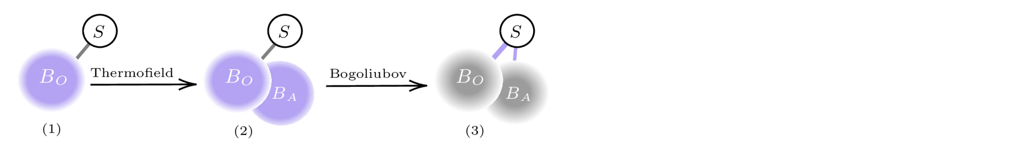
Figure 1: Schematic of the proposed method for the calculation of heat moments for a given system $S$ coupled to a bath $B$, first subjected to a thermofield doubling on $B$ (1 $\rightarrow$ 2), obtaining $B_{O}$ (real) and $B_{A}$ (auxiliary) (Eq.(5)). Second, a Bogoliubov transformation (2 $\rightarrow$ 3) that squeezes the bath modes to vacuum state $\phi$ (Eq.(7)) while transferring the temperature information in the corresponding spectral densities.

Purification scheme.—The form of Eq. (4) poses two apparent obstacles to a direct numerical evaluation of $\chi(\lambda,t)$. The first stems from initialization of the thermal state of the bath $\hat{\pi}_{\beta}$, which can be achieved by imaginary time evolution starting from a maximally mixed state. This procedure is costly for certain representations of the bath modes, including the 1D chain geometry pertinent for TEDOPA. In the language of tensor networks, imaginary-time evolution generates a large bond dimension (which is a measure of correlations) of the matrix-product operator (MPO) [58, 59, 60, 61] representing the bath state, especially for low, nonzero temperatures. Second, the propagator in Eq. (4) is dressed by the counting field via the operators $e^{\pm i\lambda H_{B}}$, leading to a non-unitary (trace-decreasing) overall time evolution, which can be unstable for standard tensor-network methods.

We sidestep both these issues using the thermofield approach [62, 63] that introduces a decoupled (otherwise identical) auxiliary environment (denoted by $A$) to the original system-bath Hamiltonian (denoted as $S$ and $O$ respectively) [64, 65]; see Fig. 1 for an illustration. Bath $A$ consists of modes $\hat{b}_{\nu}$ of frequency $-\omega_{\nu}$ that correspond to every mode $\hat{a}_{\nu}$ of frequency $\omega_{\nu}$ in bath $O$. This effectively doubles the Hilbert space of the bath, akin to a purification scheme. The total Hamiltonian in (2) is then transformed to,

$$\tilde{H}(t)=\hat{H}(t)-\hat{H}_{B,A},\quad\hat{H}_{B,A}=\sum\nolimits_{\nu}\omega_{\nu}\hat{b}^{\dagger}_{\nu}\hat{b}_{\nu}.$$ (5)

The initial state of bath $O$ which is a Gaussian state, $\hat{\pi}_{\beta}$, then gets mapped to a pure state in the extended Hilbert space of $OA$ (original + auxiliary), referred to as the ‘thermofield double’ or ‘thermal vacuum’ state: $\tilde{\tau}_{\beta}=|\psi(\beta)\rangle_{\text{\tiny$OA$}}\langle\psi(\beta)|_{\text{\tiny$OA$}}$. The thermofield transformation ensures that

$$\text{Tr}_{A}[\tilde{\tau}_{\beta}]=\hat{\pi}_{\beta}=\frac{e^{-\beta(\hat{H}_{B}-\mu\hat{N})}}{\text{Tr}[e^{-\beta(\hat{H}_{B}-\mu\hat{N})}]}.$$ (6)

Here, for generality, we have included a chemical potential $\mu$ coupled to the particle number $\hat{N}$ of the bath. The purification, which is a linear operation, preserves the Gaussianity of the state $\tilde{\tau}_{\beta}$. Now, there always exists a Bogoliubov transformation [66, 67, 68], $\mathcal{G}_{\text{\tiny$\beta$}}$, that squeezes $\tilde{\tau}_{\beta}$ to the vacuum state of $OA$:

$$\tilde{\Phi}=\mathcal{G}_{\text{\tiny{\hbox{\beta}}}}[\tilde{\tau}_{\text{\tiny{\hbox{\beta}}}}]=\bigotimes_{\nu}\,\phi_{\nu,O}\otimes\phi_{\nu,A}$$ (7)

where we denote the zero occupation state of mode $\nu$ as $\phi_{\nu}=|0_{\nu}\rangle\langle 0_{\nu}|$. The transformation $\mathcal{G}_{\beta}$ is canonical, i.e. it preserves the bosonic or fermionic (anti-)commutation relations, and it can be shown [69, 70] that $\mathcal{G}_{\beta}[\bullet]=e^{-i\hat{G}_{\beta}}\bullet e^{i\hat{G}_{\beta}}$ is generated by the Hermitian operator $\hat{G}_{\text{\tiny$\beta$}}=-i\sum\nolimits_{\nu}\theta_{\text{\tiny$\beta$},\nu}(\hat{a}_{\nu}^{\dagger}\hat{b}_{\nu}^{\dagger}-\hat{b}_{\nu}\hat{a}_{\nu})$. This transformation mixes the modes of the $O$ and $A$ baths as follows:

$$\mathcal{G}_{\text{\tiny$\beta$}}[\hat{a}_{\nu}]=u_{\text{\tiny$\beta$},\nu}\hat{a}_{\nu}+v_{\text{\tiny$\beta$},\nu}\hat{b}_{\nu}^{\dagger},$$

$$\mathcal{G}_{\beta}[\hat{b}_{\nu}]=u_{\text{\tiny$\beta$},\nu}\hat{b}_{\nu}+(-1)^{\eta+1}v_{\text{\tiny$\beta$},\nu}\hat{a}_{\nu}^{\dagger},$$ (8)

with $v_{\text{\tiny$\beta$},\nu}=\text{sin}((-i)^{\eta}\theta_{\text{\tiny$\beta$},\nu})=\sqrt{n_{\text{\tiny$\beta$},\nu}}$ and $u_{\text{\tiny$\beta$},\nu}^{2}+(-1)^{\eta}v_{\text{\tiny$\beta$},\nu}^{2}=1$, $u_{\text{\tiny$\beta$},\nu}\geq 0$. Here, $\eta=0$ or $\eta=1$ for fermions or bosons, respectively, while the thermal occupation of the $\nu^{\rm th}$ mode is $n_{\beta,\nu}=[e^{\beta(\omega_{\nu}-\mu)}+(-1)^{\eta}]^{-1}$.

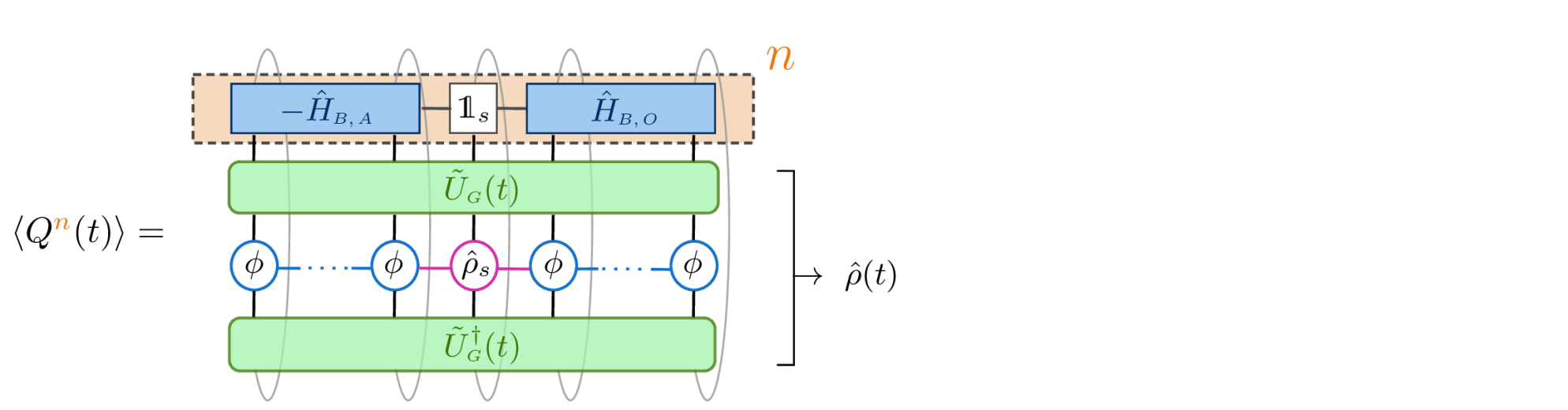
Figure 2: Diagram illustrating the evaluation of heat moments in Eq. (12). The heat operator (shaded in orange) defined in (9) is applied $n$ times to the time-evolved state $\hat{\rho}(t)$ (denoted with circles) defined on $S$ and the extended bath $OA$.

Main result.—We now introduce the ‘heat operator’ defined on $OA$,

$$\tilde{\mathcal{Q}}:=\hat{H}_{B,O}-\hat{H}_{B,A}.$$ (9)

For any Gaussian initial bath state, we prove in Appendix B that

$$\chi(\lambda,t)=\text{Tr}\left\{e^{i\lambda\tilde{\mathcal{Q}}}\,\mathcal{U}^{\text{\tiny{\hbox{G}}}}_{t}[\hat{\rho}_{\text{\tiny{\hbox{S}}}}(0)\otimes\tilde{\Phi}]\right\}.$$ (10)

Here, $\mathcal{U}^{\text{\tiny$G$}}_{t}[\bullet]=\tilde{U}_{G}(t)\bullet\tilde{U}_{G}^{\dagger}(t)$ and $\tilde{U}_{G}(t)$ is the unitary time evolution operator generated by $\tilde{H}_{G}(t)=\mathcal{G}_{\text{\tiny$\beta$}}[\tilde{H}(t)]$, which is given explicitly by

$$\tilde{H}_{G}(t)=\tilde{H}(t)+\sum_{\nu}\left(u_{\nu}g_{\nu}\hat{L}^{\dagger}\hat{a}_{\nu}+v_{\nu}g_{\nu}\hat{b}_{\nu}\hat{L}+\text{h.c.}\right).$$ (11)

It follows from Eq. (10) that

$$\langle Q^{n}(t)\rangle=\langle\tilde{\mathcal{Q}}^{n}(t)\rangle\equiv\text{Tr}\left\{\tilde{\mathcal{Q}}^{n}\,\mathcal{U}^{\text{\tiny{\hbox{G}}}}_{t}[\hat{\rho}_{\text{\tiny{\hbox{S}}}}(0)\otimes\tilde{\Phi}]\right\},$$ (12)

which states that each moment of the stochastic heat equals the corresponding moment of the heat operator $\tilde{\mathcal{Q}}(t)$, where time evolution is generated by the transformed Hamiltonian $\tilde{H}_{G}(t)$ and the expectation value is taken with respect to an initial vacuum state $\tilde{\Phi}$ of the extended $OA$ bath.

Eqs. (10) and (12) are the main results of our paper. They recast the computation of quantum heat statistics as a single-time expectation value in an extended Hilbert space, which can be tackled using standard unitary time-evolution algorithms. In particular, Eqs. (12) and (10) are now in a form that is amenable to simulation using TEDOPA. The environments $O$ and $A$ are mapped onto independent 1D chains, where each chain mapping is generated by the family of orthogonal polynomials determined by the couplings ($u_{\nu}g_{\nu}$ or $v_{\nu}g_{\nu}$) entering the linear interaction Hamiltonian in Eq. (11). In this basis, the modified Hamiltonian $\tilde{H}_{G}$ involves only two-body, nearest-neighbor interaction terms. Moreover, assuming $\hat{\rho}_{S}(0)=|\psi_{S}(0)\rangle\langle\psi_{S}(0)|$ is pure, the initial state of the entire setup is pure and can be represented by a trivial MPS (i.e. with bond dimension one). Finally, the heat operator and its powers $\tilde{\mathcal{Q}}^{n}$ are trivial MPOs. Evaluation of the heat moments using Eq. (12) therefore requires only standard MPS time evolution followed by a simple expectation value, as depicted in Fig. 2. Extracting the full characteristic function from Eq. (10) requires an additional (one-sided) unitary time evolution $e^{i\lambda\tilde{\mathcal{Q}}}$ before taking the expectation value, which can again be achieved using standard time evolution techniques. Here, we leave the analysis of the full characteristic function for future work, and extract the moments directly using Eq. (12).

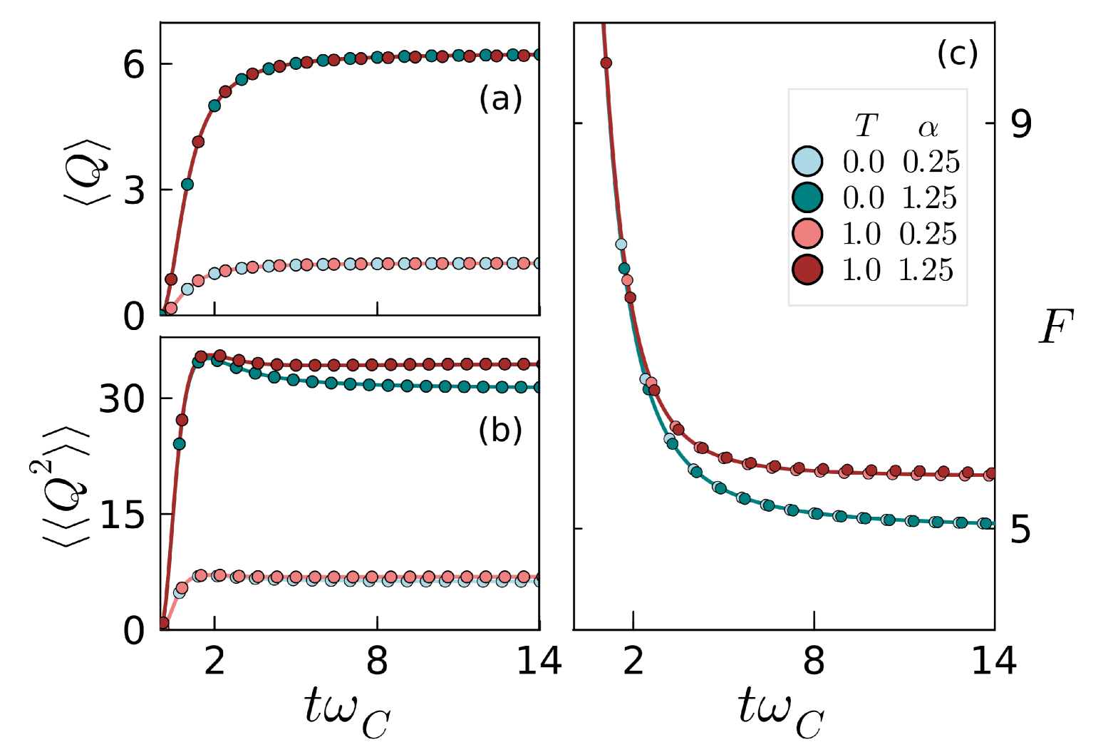
Figure 3: Evolution of (a) mean, (b) variance, and (c) Fano factor of heat fluctuations in the independent-boson model ($\epsilon_{0}=0,\ \Delta=1,\ \omega_{c}=5$). The initial state of the spin is the $|+\rangle$ eigenstate of $\hat{S}_{x}$. Exact solutions for this model are plotted as solid lines.

Heat statistics in the spin-boson model.—As an example implementation of our method, we consider the Ohmic spin-boson model, which describes a two-level system (spin) interacting with a harmonic-oscillator bath and stands as a cornerstone of quantum dissipation theory [53]. It is described by the Hamiltonian $\hat{H}=\epsilon_{0}\hat{S}_{z}+\Delta\hat{S}_{x}+\sum_{\nu}\omega_{\nu}\hat{a}^{\dagger}_{\nu}\hat{a}_{\nu}+\hat{S}_{x}\otimes\sum\nolimits_{\nu}g_{\nu}(\hat{a}_{\nu}+\hat{a}^{\dagger}_{\nu})$, with $\hat{S}_{x,z}$ the spin-1/2 angular momentum operators and $\hat{a}_{\nu}$ the bosonic annihilation operator for the bath mode $\nu$. The two-level system can be understood as representing the two lowest-energy states of a particle confined in a double-well potential. The energy splitting, $\epsilon_{0}$, corresponds to an asymmetry between the wells, while the tunneling amplitude, $\Delta$, quantifies the coupling between the two localized states due to tunneling through the central barrier. We assume the bath spectral density to be of Ohmic type, $J(\omega)=2\alpha\omega\,\text{exp}(-\omega/\omega_{C})$, with $\alpha$ a dimensionless coupling strength and $\omega_{C}$ a cutoff frequency.

We first consider the independent-boson limit with $\epsilon_{0}=0$. The heat statistics in this case are exactly solvable and independent of the initial spin state [44], and we use these exact results to verify our method. Fig. 3 shows the time evolution of the mean $\langle Q(t)\rangle$ and variance $\langle\langle Q^{2}(t)\rangle\rangle$ for the independent-boson model, taking $\Delta=1$ and the initial state $\hat{\rho}_{S}(0)=|+\rangle\langle+|$, where $\hat{S}_{x}|+\rangle=|+\rangle$. We have used both time-evolving block decimation [71] and time-dependent variational principle [72] algorithms for MPS time evolution in the chain geometry, finding the latter has somewhat better performance. We see excellent agreement between our numerical data and the exact solution at all times for both zero and finite temperatures, and both weak ($\alpha<1$) and strong ($\alpha\gtrsim 1$) bath couplings. In particular, we verify that the Fano factor, $F(t)=\langle\langle Q^{2}(t)\rangle\rangle/\langle Q(t)\rangle$, is independent of $\alpha$, in agreement with the exact solution which predicts that all heat cumulants are proportional to $\alpha$ [44].

Next, we study the nonintegrable regime ($\epsilon_{0}=1$ and $\Delta=0$) of the Ohmic spin-boson model. In this case, the spin undergoes a quantum phase transition from the delocalized to the localized regime in the $\hat{S}_{x}$ eigenbasis when the bath coupling constant $\alpha$ exceeds the critical value $\alpha_{c}=1+\mathcal{O}(\epsilon_{0}/\omega_{c})$ [52, 73]. In Fig. 4, we again take the initial spin state to be the $|+\rangle$ eigenstate of $\hat{S}_{x}$, and examine the heat statistics for coupling strengths on either side of the critical point. For both zero and finite temperatures, the mean and variance of the heat is larger for stronger coupling. For couplings beyond the critical point, the heat statistics approach the predictions of the independent-boson model, which is expected since the spin dynamics is effectively frozen and the energetics are dominated by the system-bath interaction. At weaker coupling, the mean heat quickly equilibrates while the variance exhibits two well separated timescales: a fast increase followed by a slow decrease, with the latter dictated by the equilibration of the spin. These features are most evident in the Fano factor, which depends significantly on both temperature and coupling strength, in contrast to the independent-boson behavior of Fig. 3.

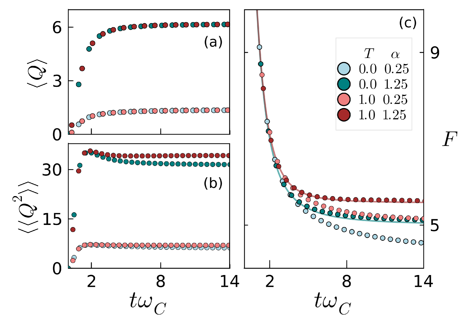
Figure 4: Evolution of (a) mean, (b) variance, and (c) Fano factor of heat fluctuations in the spin-boson model ($\epsilon_{0}=1,\ \Delta=0,\ \omega_{C}=5$). The initial state of the spin is the $|+\rangle$ eigenstate of $\hat{S}_{x}$. Curves from Fig. 3 are shown as solid colored lines for reference.

Discussion.—Heat exchange is a crucial aspect of open quantum dynamics, but its characterization in the strong-coupling regime has proved elusive, partly because of the two-time measurement implicit in its definition. We bypass this issue by defining the heat operator (9), in terms of which the heat statistics can be extracted from dynamical pure-state expectation values on an extended Hilbert space, as in Eq. (12). This approach is especially useful when only a few moments of the heat distribution are needed, since it avoids the need to numerically differentiate or Fourier transform with respect to a counting field. Nevertheless, the full counting-field dependent characteristic function can also be mapped out using Eq. (10). It is straightforward to cast this as a survival amplitude, $\chi(\lambda,t)=\langle\Psi_{G}(t)|e^{i\lambda\mathcal{\tilde{Q}}}|\Psi_{G}(t)\rangle$, where $|\Psi_{G}(t)\rangle=\tilde{U}_{G}(t)|\psi_{S}(0)\rangle\otimes|\tilde{\Phi}\rangle$ and $\tilde{\Phi}=|\tilde{\Phi}\rangle\langle\tilde{\Phi}|$ is the initial vacuum state of $OA$. Once the state $|\Psi_{G}(t)\rangle$ is prepared for a given time $t$, computing $\chi(\lambda,t)$ requires only a single unitary time evolution over the counting field $\lambda$. Since it is defined via a thermofield purification, this survival amplitude differs from the overlap that appears when measuring heat by an ancilla-assisted interferometric protocol [74]. Such ancilla-based protocols have previously been exploited in tensor-network simulations of the characteristic functions for work [75] or charge [76] fluctuations in many-body lattice systems.

Our preliminary analysis of the spin-boson model in Fig. 4 indicates nontrivial dynamics of the Fano factor at moderately weak coupling strengths, due to competition between the spin energy splitting and the system-bath interaction. In future work, we will apply our method to perform a detailed investigation of heat fluctuations across the entire phase diagram, covering a range of temperatures and initial system states. Note that, while we have only considered pure initial preparations for the system, mixtures are easily incorporated by averaging Eqs. (10) or (12) over the initial distribution in $\hat{\rho}_{S}(0)$. The heat operator approach can be further generalized to describe multiple baths in the presence of chemical or thermal gradients, including interactions or driving within the open quantum system, by adding more chains to describe each bath. The same purification technique can also be adapted to other thermodynamic quantities such as particle-current statistics. Our work thus substantially expands the toolkit of quantum stochastic thermodynamics into the strong-coupling regime.

Data availability.—The open-source code used in our simulations is based on the ITensor library [77] and can be accessed at Ref. [78].

Acknowledgments.—We thank Saulo V. Moreira, Antonio Verdú, and Hari Kumar Yadalam for helpful discussions and suggestions regarding the manuscript. We warmly acknowledge Kesha for the use of her computational resources. This project is co-funded by the European Union (Quantum Flagship project ASPECTS, Grant Agreement No. 101080167) and UK Research and Innovation (UKRI). Views and opinions expressed are, however those of the authors only and do not necessarily reflect those of the European Union, Research Executive Agency or UKRI. Neither the European Union nor UKRI can be held responsible for them. M.T.M. is supported by a Royal Society University Research Fellowship. J.P. acknowledges support from grant TED2021-130578B-I00 and grant PID2021-124965NB-C21 funded by MICIU/AEI/10.13039/501100011033 and by the “European Union NextGeneration EU/PRTR”.

Supplemental Materials for “Heat operator approach to quantum stochastic thermodynamics in the strong-coupling regime”

Appendix A Derivation of Eq. (4)

We assume an initial product state of the system and the bath, $\hat{\rho}(0)=\hat{\rho}_{\text{\tiny$S$}}(0)\otimes\hat{\pi}_{\beta}$ where the thermal state $\hat{\pi}_{\beta}$ is of the form (6). In the 2-point measurement scheme, the probability distribution of fluctuations of heat ($Q(t)$) is given by

$$P(Q,t)=\sum_{m,n}\text{Tr}\{\Pi_{n}\mathcal{U}_{t}[\Pi_{m}\hat{\rho}(0)\Pi_{m}]\}\delta(Q+E_{m}-E_{n}).$$

Thus the characteristic function of heat is given by

$$\chi(u,t) =\int dQP(Q)\,e^{i\lambda Q}$$ (S1)

$$=\sum_{m,n}\text{Tr}\{\Pi_{n}\mathcal{U}_{t}[\Pi_{m}\hat{\rho}(0)\Pi_{m}]\}\,e^{i\lambda(E_{n}-E_{m})}$$ (S2)

$$=\text{Tr}\{\sum_{n}e^{i\lambda E_{n}}\Pi_{n}\,\mathcal{U}_{t}[\sum_{m}e^{-i\lambda E_{m}}\Pi_{m}\,\hat{\rho}_{\text{\tiny$S$}}(0)\otimes\hat{\pi}_{\beta}\,\Pi_{m}]\}$$ (S3)

$$=\text{Tr}\{\sum_{n}e^{i\lambda E_{n}}\Pi_{n}\,\mathcal{U}_{t}[\sum_{m}e^{-i\lambda E_{m}}\Pi_{m}\hat{\rho}(0)]\}$$ (S4)

$$=\text{Tr}\left\{e^{iu\hat{H}_{B}}\,\mathcal{U}_{t}[e^{-i\lambda\hat{H}_{B}}\hat{\rho}(0)]\right\}$$ (S5)

Appendix B Verification of Eq. (12)

The key ingredient required in characterizing fluctuating heat exchange is the characteristic function denoted by $\chi(\lambda,t)$, that has the standard form in (4). In this section, we begin with our proposed modified characteristic function expression (10) and derive (4). This, in turn, will prove the primary statement of the article stated in Eq. (12).

We start by expanding (10):

$$\chi(\lambda,t) = \text{Tr}\left\{e^{i\lambda\tilde{\mathcal{Q}}}\,\mathcal{U}^{\text{\tiny$G$}}_{t}[\hat{\rho}_{\text{\tiny$S$}}(0)\otimes\tilde{\Phi}]\right\}$$ (S6)

$$= \text{Tr}\left\{e^{i\lambda\tilde{\mathcal{Q}}}\,\tilde{U}_{G}(t)\,(\hat{\rho}_{\text{\tiny$S$}}(0)\otimes\tilde{\Phi})\,\tilde{U}_{G}^{\dagger}(t)\,\right\}\qquad$$

$$= \text{Tr}\left\{e^{i\lambda\tilde{\mathcal{Q}}}\,\tilde{U}_{G}(t)\,e^{-i\lambda\tilde{\mathcal{Q}}}\,(\hat{\rho}_{\text{\tiny$S$}}(0)\otimes\tilde{\Phi})\,\tilde{U}^{\dagger}_{G}(t)\,\right\}\qquad\left[\because\tilde{\mathcal{Q}}(\hat{\rho}_{\text{\tiny$S$}}(0)\otimes\tilde{\Phi})=0\right]$$

$$= \text{Tr}\left\{e^{i\lambda\tilde{\mathcal{Q}}}\,\mathcal{G}_{\text{\tiny$\beta$}}[\tilde{U}(t)]\,e^{-i\lambda\tilde{\mathcal{Q}}}\,(\hat{\rho}_{\text{\tiny$S$}}(0)\otimes\tilde{\Phi})\,\mathcal{G}_{\text{\tiny$\beta$}}[\tilde{U}^{\dagger}(t)]\,\right\},$$

where $\tilde{U}(t)=\overset{\leftarrow}{\rm T}{\rm exp}[-i\int_{0}^{t}dt^{\prime}\,\tilde{H}(t^{\prime})]$ is the time-evolution operator generated by $\tilde{H}(t)$, as defined in Eq. (5). Note that $\hat{G}_{\text{\tiny$\beta$}}=-i\sum\nolimits_{\nu}\theta_{\text{\tiny$\beta$},\nu}(\hat{a}_{\nu}^{\dagger}\hat{b}_{\nu}^{\dagger}-\hat{b}_{\nu}\hat{a}_{\nu})$ commutes with $\tilde{\mathcal{Q}}$, i.e., $[\hat{G}_{\text{\tiny$\beta$}},\tilde{\mathcal{Q}}]=0$. Then one can write for any operator $\hat{x}$,

$$e^{i\lambda\mathcal{\tilde{Q}}}\mathcal{G}_{\text{\tiny{\hbox{\beta}}}}[\hat{x}]e^{-i\lambda\mathcal{\tilde{Q}}}=\mathcal{G}_{\text{\tiny{\hbox{\beta}}}}[e^{i\lambda\mathcal{\tilde{Q}}}\,\hat{x}\,e^{-i\lambda\mathcal{\tilde{Q}}}].$$ (S7)

Using (S7) and the thermal vacuum state $\tilde{\tau}_{\text{\tiny$\beta$}}=\mathcal{G}_{\text{\tiny$\beta$}}^{-1}[\tilde{\Phi}]$ from Eq. (7), we get

$$\chi(\lambda,t) = \text{Tr}\left\{\mathcal{G}_{\text{\tiny$\beta$}}[e^{i\lambda\tilde{\mathcal{Q}}}\,\tilde{U}(t)\,e^{-i\lambda\tilde{\mathcal{Q}}}]\,(\hat{\rho}_{\text{\tiny$S$}}(0)\otimes\tilde{\Phi})\,\mathcal{G}_{\text{\tiny$\beta$}}[\tilde{U}^{\dagger}(t)]\,\right\}$$ (S8)

$$= \text{Tr}\left\{e^{i\lambda\tilde{\mathcal{Q}}}\,\tilde{U}(t)\,e^{-i\lambda\tilde{\mathcal{Q}}}\,(\hat{\rho}_{\text{\tiny$S$}}(0)\otimes\tilde{\tau}_{\text{\tiny$\beta$}})\,\tilde{U}^{\dagger}(t)\right\}$$ (S9)

In the following, we use $\tilde{H}(t)=\hat{H}(t)-\hat{H}_{B,A}$ (Eq. (5)) and that $[\hat{H},\hat{H}_{B,A}]=[\hat{H}_{B,O},\hat{H}_{B,A}]=0$, from which it follows that $\tilde{U}(t)=\hat{U}(t)e^{it\hat{H}_{B,A}}=e^{it\hat{H}_{B,A}}\hat{U}(t)$, where $\hat{U}(t)=\overset{\leftarrow}{\rm T}{\rm exp}[-i\int_{0}^{t}dt^{\prime}\,\hat{H}(t^{\prime})]$ is generated by the original Hamiltonian $\hat{H}(t)$ in Eq. (2). Finally, tracing out the auxiliary bath $A$ (Eq. (6)), we recover the standard expression for heat characteristic function in Eq. (4).

$$\chi(\lambda,t) = \text{Tr}\left\{e^{i\lambda(\hat{H}_{B,O}-\hat{H}_{B,A})}\,\tilde{U}(t)\,e^{-i\lambda(\hat{H}_{B,O}-\hat{H}_{B,A})}\,(\hat{\rho}_{\text{\tiny$S$}}(0)\otimes\tilde{\tau}_{\text{\tiny$\beta$}})\,\tilde{U}^{\dagger}(t)\,\right\}$$ (S10)

$$= \text{Tr}_{O}\left\{e^{i\lambda\hat{H}_{B,O}}\,\hat{U}(t)\,e^{-i\lambda\hat{H}_{B,O}}\,(\hat{\rho}_{\text{\tiny$S$}}(0)\otimes\text{Tr}_{A}\left\{\tilde{\tau}_{\text{\tiny$\beta$}}\right\})\,\hat{U}^{\dagger}(t)\,\right\}$$

$$= \text{Tr}_{O}\left\{e^{i\lambda\hat{H}_{B,O}}\,\hat{U}(t)\,e^{-i\lambda\hat{H}_{B,O}}\,(\hat{\rho}_{\text{\tiny$S$}}(0)\otimes\hat{\pi}_{\text{\tiny$\beta$}})\,\hat{U}^{\dagger}(t)\,\right\}$$

$$= \text{Tr}_{O}\left\{e^{i\lambda\hat{H}_{B,O}}\,\mathcal{U}_{t}[e^{-i\lambda\hat{H}_{B,O}}\hat{\rho}(0)]\right\},$$

which proves Eq. (10). Using the definition in Eq. (3), we can state that indeed the $n^{\rm th}$ moment of heat is given by,

$$\langle Q^{n}(t)\rangle=\text{Tr}\left\{\tilde{\mathcal{Q}}^{n}\,\mathcal{U}^{\text{\tiny{\hbox{G}}}}_{t}[\hat{\rho}_{\text{\tiny{\hbox{S}}}}(0)\otimes\tilde{\Phi}]\right\}.$$ (S11)

This concludes the proof of our main result in Eq. (12).

Appendix C TEDOPA

Given that the environment comprises reservoirs, each characterized by a spectral density $J_{j}(\omega)$, TEDOPA presents an exact unitary transformation $U_{j,n}(\omega)$ mapping the continuum of bosonic or fermionic modes to discrete semi-infinite chains (each corresponding to a single bath) with only nearest-neighbor interactions. For each bath $B_{j}$, $U_{j,n}(\omega)=g_{j}(\omega)p_{j,n}(\omega)$ is defined such that $\int d\omega\,U_{j,m}(\omega)U_{j,n}(\omega)=\delta_{mn}$. That is, $\{p_{j,n}(\omega)\}_{n}$ is the set of orthogonal polynomials with respect to the measure $d\mu(\omega)=g_{j}^{2}(\omega)d\omega$. The system-bath coupling strengths $g_{j}(\omega)$ (see Eq.(1)) thus determines the chain-mapped bath operators

$$\hat{b}_{j,n}=\int d\omega\,U_{j,n}(\omega)\hat{a}_{j,\omega}.$$ (S12)

The chain-mapped bath operators $\{\hat{b}_{j,n}\}$ satisfy the standard commutation relations for the respective baths. The Hamiltonian (Eq. (2)) after chain mapping (S12) becomes,

$$\hat{H}_{CM}=\hat{H}_{S}+c_{0}\hat{A}(b_{0}+b_{0}^{\dagger})+\sum_{n=0}^{\infty}\omega_{n}b_{n}^{\dagger}b_{n}+t_{n}(b_{n+1}^{\dagger}b_{n}+b_{n}^{\dagger}b_{n+1}).$$ (S13)

Here $c_{0}^{2}=\int d\mu(\omega)$ is the coupling of the system with the first site of the chain-mapped bath. The tunneling frequencies $t_{n}$ and mode frequencies $\omega_{n}$ are the recurrence coefficients corresponding to the measure $d\mu(\omega)$.

References

- Popovic et al. [2023] M. Popovic, M. T. Mitchison, and J. Goold, Proc. Roy. Soc. A 479, 20230040 (2023).
- Landi and Paternostro [2021] G. T. Landi and M. Paternostro, Rev. Mod. Phys. 93, 035008 (2021).
- Strasberg and Winter [2021] P. Strasberg and A. Winter, PRX Quantum 2, 030202 (2021).
- Aamir et al. [2025] M. A. Aamir, P. Jamet Suria, J. A. Marín Guzmán, C. Castillo-Moreno, J. M. Epstein, N. Yunger Halpern, and S. Gasparinetti, Nature Physics , 1 (2025).
- Antonio Marín Guzmán et al. [2024] J. Antonio Marín Guzmán, P. Erker, S. Gasparinetti, M. Huber, and N. Yunger Halpern, Rep. Prog. Phys. 87, 122001 (2024).
- Spiecker et al. [2023] M. Spiecker, P. Paluch, N. Gosling, N. Drucker, S. Matityahu, D. Gusenkova, S. Günzler, D. Rieger, I. Takmakov, F. Valenti, P. Winkel, R. Gebauer, O. Sander, G. Catelani, A. Shnirman, A. V. Ustinov, W. Wernsdorfer, Y. Cohen, and I. M. Pop, Nature Physics 19, 1320 (2023).
- Levy and Lostaglio [2020] A. Levy and M. Lostaglio, PRX Quantum 1, 010309 (2020).
- Kerremans et al. [2022] T. Kerremans, P. Samuelsson, and P. P. Potts, SciPost Phys. 12, 168 (2022).
- Miller et al. [2020] H. J. D. Miller, G. Guarnieri, M. T. Mitchison, and J. Goold, Phys. Rev. Lett. 125, 160602 (2020).
- Ptaszyński [2018] K. Ptaszyński, Phys. Rev. B 98, 085425 (2018).
- Agarwalla and Segal [2018] B. K. Agarwalla and D. Segal, Phys. Rev. B 98, 155438 (2018).
- Brandner et al. [2018] K. Brandner, T. Hanazato, and K. Saito, Phys. Rev. Lett. 120, 090601 (2018).
- Guarnieri et al. [2019] G. Guarnieri, G. T. Landi, S. R. Clark, and J. Goold, Phys. Rev. Research 1, 033021 (2019).
- Kalaee et al. [2021] A. A. S. Kalaee, A. Wacker, and P. P. Potts, Phys. Rev. E 104, L012103 (2021).
- Rignon-Bret et al. [2021] A. Rignon-Bret, G. Guarnieri, J. Goold, and M. T. Mitchison, Phys. Rev. E 103, 012133 (2021).
- Rivas et al. [2014] Á. Rivas, S. F. Huelga, and M. B. Plenio, Rep. Prog. Phys. 77, 094001 (2014).
- Breuer et al. [2016] H.-P. Breuer, E.-M. Laine, J. Piilo, and B. Vacchini, Rev. Mod. Phys. 88, 021002 (2016).
- Josefsson et al. [2018] M. Josefsson, A. Svilans, A. M. Burke, E. A. Hoffmann, S. Fahlvik, C. Thelander, M. Leijnse, and H. Linke, Nature Nanotechnology 13, 920 (2018).
- Josefsson et al. [2019] M. Josefsson, A. Svilans, H. Linke, and M. Leijnse, Phys. Rev. B 99, 235432 (2019).
- Talkner and Hänggi [2020] P. Talkner and P. Hänggi, Rev. Mod. Phys. 92, 041002 (2020).
- Trushechkin et al. [2022] A. S. Trushechkin, M. Merkli, J. D. Cresser, and J. Anders, AVS Quantum Science 4, 012301 (2022).
- Wang et al. [2014] J.-S. Wang, B. K. Agarwalla, H. Li, and J. Thingna, Frontiers of Physics 9, 673 (2014).
- Carrega et al. [2016] M. Carrega, P. Solinas, M. Sassetti, and U. Weiss, Phys. Rev. Lett. 116, 240403 (2016).
- Segal and Agarwalla [2016] D. Segal and B. K. Agarwalla, Annual Review of Physical Chemistry 67, 185 (2016).
- Song and Shi [2017] L. Song and Q. Shi, Phys. Rev. B 95, 064308 (2017).
- Kilgour et al. [2019] M. Kilgour, B. K. Agarwalla, and D. Segal, The Journal of Chemical Physics 150, 084111 (2019).
- Yadalam et al. [2022] H. K. Yadalam, B. K. Agarwalla, and U. Harbola, Phys. Rev. A 105, 062219 (2022).
- Prior et al. [2010] J. Prior, A. W. Chin, S. F. Huelga, and M. B. Plenio, Phys. Rev. Lett. 105, 050404 (2010).
- Prior et al. [2013] J. Prior, I. de Vega, A. W. Chin, S. F. Huelga, and M. B. Plenio, Physical Review A—Atomic, Molecular, and Optical Physics 87, 013428 (2013).
- Tamascelli et al. [2019] D. Tamascelli, A. Smirne, J. Lim, S. F. Huelga, and M. B. Plenio, Phys. Rev. Lett. 123, 090402 (2019).
- Nüßeler et al. [2020] A. Nüßeler, I. Dhand, S. F. Huelga, and M. B. Plenio, Phys. Rev. B 101, 155134 (2020).
- Strathearn et al. [2018] A. Strathearn, P. Kirton, D. Kilda, J. Keeling, and B. W. Lovett, Nature Communications 9, 3322 (2018).
- Jørgensen and Pollock [2019] M. R. Jørgensen and F. A. Pollock, Phys. Rev. Lett. 123, 240602 (2019).
- Thoenniss et al. [2023] J. Thoenniss, M. Sonner, A. Lerose, and D. A. Abanin, Phys. Rev. B 107, L201115 (2023).
- Cygorek et al. [2022] M. Cygorek, M. Cosacchi, A. Vagov, V. M. Axt, B. W. Lovett, J. Keeling, and E. M. Gauger, Nature Physics 18, 662 (2022).
- Somoza et al. [2019] A. D. Somoza, O. Marty, J. Lim, S. F. Huelga, and M. B. Plenio, Phys. Rev. Lett. 123, 100502 (2019).
- Wójtowicz et al. [2020] G. Wójtowicz, J. E. Elenewski, M. M. Rams, and M. Zwolak, Phys. Rev. A 101, 050301 (2020).
- Lotem et al. [2020] M. Lotem, A. Weichselbaum, J. von Delft, and M. Goldstein, Phys. Rev. Res. 2, 043052 (2020).
- Brenes et al. [2020] M. Brenes, J. J. Mendoza-Arenas, A. Purkayastha, M. T. Mitchison, S. R. Clark, and J. Goold, Phys. Rev. X 10, 031040 (2020).
- Purkayastha et al. [2021] A. Purkayastha, G. Guarnieri, S. Campbell, J. Prior, and J. Goold, Phys. Rev. B 104, 045417 (2021).
- Cirio et al. [2023] M. Cirio, N. Lambert, P. Liang, P.-C. Kuo, Y.-N. Chen, P. Menczel, K. Funo, and F. Nori, Phys. Rev. Res. 5, 033011 (2023).
- Esposito et al. [2009] M. Esposito, U. Harbola, and S. Mukamel, Rev. Mod. Phys. 81, 1665 (2009).
- Talkner and Hänggi [2020] P. Talkner and P. Hänggi, Rev. Mod. Phys. 92, 041002 (2020).
- Popovic et al. [2021] M. Popovic, M. T. Mitchison, A. Strathearn, B. W. Lovett, J. Goold, and P. R. Eastham, PRX Quantum 2, 020338 (2021).
- Brenes et al. [2023] M. Brenes, G. Guarnieri, A. Purkayastha, J. Eisert, D. Segal, and G. Landi, Phys. Rev. B 108, L081119 (2023).
- Shubrook et al. [2024] M. Shubrook, J. Iles-Smith, and A. Nazir, Quantum Science and Technology (2024).
- Valli et al. [2024] A. Valli, C. P. Moca, M. A. Werner, M. Kormos, Ž. Krajnik, T. Prosen, and G. Zaránd, arXiv preprint arXiv:2409.14442 (2024).
- Woods et al. [2014] M. P. Woods, R. Groux, A. W. Chin, S. F. Huelga, and M. B. Plenio, J. Math. Phys. 55, 032101 (2014).
- Tamascelli et al. [2018] D. Tamascelli, A. Smirne, S. F. Huelga, and M. B. Plenio, Phys. Rev. Lett. 120, 030402 (2018).
- Menczel et al. [2024] P. Menczel, K. Funo, M. Cirio, N. Lambert, and F. Nori, Phys. Rev. Res. 6, 033237 (2024).
- Bettmann et al. [2024] L. P. Bettmann, M. J. Kewming, G. T. Landi, J. Goold, and M. T. Mitchison, Quantum stochastic thermodynamics in the mesoscopic-leads formulation (2024), arXiv:2404.06426 [cond-mat, physics:quant-ph] .
- Leggett et al. [1987] A. J. Leggett, S. Chakravarty, A. T. Dorsey, M. P. A. Fisher, A. Garg, and W. Zwerger, Rev. Mod. Phys. 59, 1 (1987).
- Weiss [2012] U. Weiss, An Introduction to Stochastic Thermodynamics From Basic to Advanced (WORLD SCIENTIFIC, 2012).
- Breuer and Petruccione [2007] H.-P. Breuer and F. Petruccione, The Theory of Open Quantum Systems (2007).
- de Vega et al. [2015] I. de Vega, U. Schollwöck, and F. A. Wolf, Phys. Rev. B 92, 155126 (2015).
- Colla and Breuer [2022] A. Colla and H.-P. Breuer, Phys. Rev. A 105, 052216 (2022).
- Note [1] Our approach aligns with the framework of Ref. [20] so long as the system-environment interaction is assumed to be switched on and off at the beginning and end of the evolution time , which is fully consistent with our assumption of a product initial condition.
- Zwolak and Vidal [2004] M. Zwolak and G. Vidal, Phys. Rev. Lett. 93, 207205 (2004).
- Verstraete et al. [2004] F. Verstraete, J. J. García-Ripoll, and J. I. Cirac, Phys. Rev. Lett. 93, 207204 (2004).
- Hartmann et al. [2009] M. J. Hartmann, J. Prior, S. R. Clark, and M. B. Plenio, Phys. Rev. Lett. 102, 057202 (2009).
- [61] I. P. McCulloch, Infinite size density matrix renormalization group, revisited.
- Takahashi and Umezawa [1996] Y. Takahashi and H. Umezawa, Int. J. Mod. Phys. B 10, 1755 (1996).
- Das [1989] A. Das, Physica A: Statistical Mechanics and its Applications 158, 1 (1989).
- Karrasch et al. [2012] C. Karrasch, J. H. Bardarson, and J. E. Moore, Phys. Rev. Lett. 108, 227206 (2012).
- de Vega and Bañuls [2015] I. de Vega and M.-C. Bañuls, Phys. Rev. A 92, 052116 (2015).
- Bogoljubov et al. [1958] N. N. Bogoljubov, V. V. Tolmachov, and D. V. Širkov, Fortschritte der Physik 6, 605 (1958).
- Balian and Brezin [1969] R. Balian and E. Brezin, Il Nuovo Cimento B (1965-1970) 64, 37 (1969).
- Nam et al. [2016] P. T. Nam, M. Napiórkowski, and J. P. Solovej, Journal of Functional Analysis 270, 4340 (2016).
- Martino et al. [1996] S. D. Martino, S. D. Siena, and G. Vitiello, Int. J. Mod. Phys. B 10, 1615 (1996).
- Celeghini et al. [1998] E. Celeghini, S. De Martino, S. De Siena, A. Iorio, M. Rasetti, and G. Vitiello, Physics Letters A 244, 455 (1998).
- Vidal [2004] G. Vidal, Phys. Rev. Lett. 93, 040502 (2004).
- Haegeman et al. [2011] J. Haegeman, J. I. Cirac, T. J. Osborne, I. Pižorn, H. Verschelde, and F. Verstraete, Phys. Rev. Lett. 107, 070601 (2011).
- Bulla et al. [2003] R. Bulla, N.-H. Tong, and M. Vojta, Phys. Rev. Lett. 91, 170601 (2003).
- Goold et al. [2014] J. Goold, U. Poschinger, and K. Modi, Phys. Rev. E 90, 020101 (2014).
- Johnson et al. [2016] T. H. Johnson, F. Cosco, M. T. Mitchison, D. Jaksch, and S. R. Clark, Phys. Rev. A 93, 053619 (2016).
- Samajdar et al. [2024] R. Samajdar, E. McCulloch, V. Khemani, R. Vasseur, and S. Gopalakrishnan, Phys. Rev. Lett. 133, 240403 (2024).
- Fishman et al. [2022] M. Fishman, S. White, and E. M. Stoudenmire, SciPost Physics Codebases , 004 (2022).
- [78] ASPECTS code repository, https://github.com/aspects-quantum/TFlucn_tedopa.git.