Energy Matching: Unifying Flow Matching and Energy-Based Models for Generative Modeling

Abstract

Generative models often map noise to data by matching flows or scores, but these approaches become cumbersome for incorporating partial observations or additional priors. Inspired by recent advances in Wasserstein gradient flows, we propose Energy Matching, a framework that unifies flow-based approaches with the flexibility of energy-based models (EBMs). Far from the data manifold, samples move along curl-free, optimal transport paths from noise to data. As they approach the data manifold, an entropic energy term guides the system into a Boltzmann equilibrium distribution, explicitly capturing the underlying likelihood structure of the data. We parameterize this dynamic with a single time-independent scalar field, which serves as both a powerful generator and a flexible prior for effective regularization of inverse problems. Our method substantially outperforms existing EBMs on CIFAR-10 generation (FID $3.97$ compared to $8.61$), while retaining the simulation-free training of transport-based approaches away from the data manifold. Additionally, we exploit the flexibility of our method and introduce an interaction energy for diverse mode exploration. Our approach focuses on learning a static scalar potential energy—without time conditioning, auxiliary generators, or additional networks—marking a significant departure from recent EBM methods. We believe that this simplified framework significantly advances EBMs capabilities and paves the way for their broader adoption in generative modeling across diverse domains.

1 Introduction

Figure 1: Shown are trajectories (green lines) of samples traveling from a noise distribution (black dots; here, a Gaussian mixture model) to a data distribution (blue dots; here, two moons as in (Tong et al., 2023)) under four different methods: Action Matching (Neklyudov et al., 2023), Flow Matching (OT-CFM) (Tong et al., 2023), EBMs trained via contrastive divergence (Hinton, 2002), and our proposed Energy Matching. We highlight several individual trajectories in red to illustrate their distinct behaviors. Both Action Matching and Flow Matching learn time-dependent transports and are not trained for traversing the data manifold. Conversely, EBMs and Energy Matching are driven by time-independent fields that can be iterated indefinitely, allowing trajectories to navigate across modes. While samples from EBMs often require additional steps to equilibrate (see, e.g., the visible mode collapses that slow down sampling from the data manifold), Energy Matching directs samples toward the data distribution in “straight” paths, without hindering the exploration of the data manifold.

Many generative models learn a mapping from a simple, easy-to-sample distribution (e.g., a Gaussian) to the data distribution. They do so by approximating the optimal transport (OT) map—such as in flow matching (Lipman et al., 2023; Liu et al., 2023; Tong et al., 2023) — or via iterative noising-and-denoising schemes, as in diffusion models (Ho et al., 2020; Song et al., 2021). Besides being highly effective at sample generation, diffusion and flow-based models have also been used as priors to regularize ill-posed inverse problems (Chung et al., 2023; Mardani et al., 2024; Ben-Hamu et al., 2024). However, these models do not capture the unconditional data score explicitly, and instead model the score of smoothed manifolds at different noise levels. The measurement likelihood, on the other hand, is not tractable on these smoothed manifolds. As a result, existing approaches repeatedly shuttle between noised and data distributions, leading to crude approximations of complex, intractable terms Daras et al. (2024). For instance, DPS (Chung et al., 2023) approximates an intractable integral using a single sample. More recently, D-Flow (Ben-Hamu et al., 2024) optimizes the initial noise by differentiating through the simulated trajectory. To the best of our knowledge, these models lack a direct way to navigate the data manifold in search of the optimal solution without repeatedly transitioning between noised and data distributions.

EBMs (Hopfield, 1982; Hinton, 2002; LeCun et al., 2006) provide an alternative approach for approximating the data distribution by learning a scalar-valued function $E(x)$ that specifies an unnormalized density $p(x)\propto\exp\left(-E(x)\right)$. Rather than explicitly mapping noise samples onto the data manifold, EBMs assign low energies to regions of high data concentration and high energy elsewhere. This defines a Boltzmann distribution, from which one can sample by, for instance, Langevin sampling. In doing so, EBMs explicitly retain the likelihood information in $E(x)$. This likelihood information can then be leveraged in conditional generation (e.g., to solve inverse problems), possibly together with additional priors by simply adding their energy terms (Du and Mordatch, 2019). Moreover, direct examination of local curvature on the data manifold—allows the computation of local intrinsic dimension (LID) (an important proxy for data complexity)—whereas diffusion models can only approximate such curvature in the proximity of noise samples.

Despite the theoretical elegance of using a single, time-independent scalar energy, practical EBMs have historically suffered from poor generation quality, falling short of the performance of diffusion or flow matching models. Traditional methods (Song and Kingma, 2021) for training EBMs, such as contrastive divergence via Markov chain Monte Carlo (MCMC) or local score-based approaches (Song and Ermon, 2019), often fail to adequately explore the energy landscape in high-dimensional spaces, leading to instabilities and mode collapse. Consequently, many methods resort to time-conditioned ensembles (Gao et al., 2021), hierarchical latent ensembles (Cui and Han, 2024), or combine EBMs with separate generator networks (Guo et al., 2023; Zhang et al., 2024), thereby requiring significantly higher parameter counts and training complexity. Although multi-network approaches can improve sample quality, they inflate parameter counts by redundantly learning the same features across multiple networks, compromising the shared statistical strength of a unified feature set and the flexibility of time-independent models.

Contributions.

In this work, we propose Energy Matching, a two-regime training strategy that combines the strengths of EBMs and flow matching; see Figure˜1. When samples lie far from the data manifold, they are transported efficiently toward the data. Once near the data manifold, the flow transitions into Langevin steps governed by an internal energy component, enabling precise exploration of the Boltzmann-like density well around the data distribution. This straightforward approach produces a time-independent scalar energy field whose gradient both accelerates sampling and shapes the final density well—via a contrastive objective that directly learns the score at the data manifold—yet remains efficient and stable to train. Empirically, our method significantly outperforms existing EBMs on CIFAR-10 generation (FID $3.97$ vs. $8.61$) and compares favorably to flow-matching and diffusion models, without auxiliary generators or time-dependent EBM ensembles. Our proposed process complements the advantages of flow matching with an explicit likelihood modeling, enabling traversal of the data manifold without repeatedly shuffling between noise and data distributions. This simplifies both inverse problem solving and controlled generations under a prior. In addition, to encourage diverse exploration of the data distribution, we showcase how repulsive interaction energies can be easily and effectively incorporated. Finally, we also showcase how analyzing the learned energy reveals insight on the LID of the data with fewer approximations than diffusion models.

2 Energy matching

In this section, we show how a scalar potential $V(x)$ can simultaneously provide an optimal-transport-like flow from noise to data while also yielding a Boltzmann distribution that explicitly captures the unnormalized likelihood of the data.

The Jordan–Kinderlehrer–Otto (JKO) scheme.

The starting point of our approach is the JKO scheme (Jordan et al., 1998), which is the basis of the success of numerous recent generative models (Xu et al., 2023; Terpin et al., 2024; Choi et al., 2024). The JKO scheme describes the discrete-time evolution of a probability distribution $\rho_{t}$ along energy-minimizing trajectories in the Wasserstein space,

$$\rho_{t+\Delta t}=\arg\min_{\rho}\underbrace{\frac{W_{2}^{2}\left(\rho,\rho_{t}\right)}{2\Delta t}}_{\text{Transport Cost}}+\underbrace{\int V_{\theta}(x)\mathrm{d}\rho(x)}_{\text{Potential Energy}}+\underbrace{\varepsilon(t)\int\rho(x)\log\rho(x)\mathrm{d}x}_{\text{Internal Energy (-\text{Entropy)}}}.$$ (1)

Here, $\theta$ denotes the learnable parameters of the scalar potential $V_{\theta}(x)$, and $\varepsilon(t)$ is a temperature-like parameter tuning the entropic term. The transport cost is given by the Wasserstein distance,

$$W_{2}^{2}(\rho,\rho_{t})=\min_{\gamma\in\Gamma(\rho,\rho_{t})}\int_{\mathbb{R}^{d}\times\mathbb{R}^{d}}\norm{x-x_{t}}^{2}\mathrm{d}\gamma(x,x_{t}),$$ (2)

where $\Gamma(\rho,\rho_{t})$ is the set of couplings between $\rho$ and $\rho_{t}$, i.e., the set of probability distributions on $\mathbb{R}^{d}\times\mathbb{R}^{d}$ with marginals $\rho$ and $\rho_{t}$. Here, $d$ is the dimensionality of the data. Henceforth, we call OT coupling any $\gamma_{t}$ that yields the minimum in (2). When $\gamma_{t}=(\mathrm{id},T)_{\#}\rho$, i.e., it is the pushforward of the map $x\mapsto(x,T(x))$ for some function $T$, we say that $T$ is an OT map from $\rho$ to $\rho_{t}$.

Differently from most literature, we consider $\varepsilon(t)$ to be dependent on time and study the behavior of Equation˜1 as $t\to\infty$. To fix the ideas, consider, for instance, a linear scheduling:

$$\varepsilon(t)=\begin{cases}0,&0\leq t<\operatorname{\tau^{\ast}},\\ \varepsilon_{\max}\frac{t-\operatorname{\tau^{\ast}}}{1-\operatorname{\tau^{\ast}}},&\operatorname{\tau^{\ast}}\leq t\leq 1,\\ \varepsilon_{\max},&t\geq 1.\end{cases}$$ (3)

First-order optimality conditions.

We follow the approach in Terpin et al. (2024) and study (1) at each time $t$ via its first-order optimality conditions (Lanzetti et al., 2024, 2025):

$$\frac{1}{\Delta t}(x-y)+\nabla_{x}V_{\theta}(x)+\varepsilon(t)\nabla_{x}\log\rho_{t}(x)=0,\qquad(x,y)\in\mathrm{supp}(\gamma_{t})$$ (4)

where $\gamma_{t}$ is an OT plan between the distributions $\rho_{t}$ and $\rho_{t+\Delta t}$ and $\mathrm{supp}(\gamma_{t})$ is the support of $\gamma_{t}$. That is, this condition has to hold for all pairs of points in the support of $\rho_{t}$ and $\rho_{t+\Delta t}$ that are coupled by OT. Intuitively, analyzing (4) provides us with two key insights:

1. For times $t<\tau^{*}$, $\varepsilon(t)=0$ and (4) becomes

   $$\frac{1}{\Delta t}(x-y)+\nabla_{x}V_{\theta}(x)=0\qquad(x,y)\in\mathrm{supp}(\gamma_{t}).$$ (5)

   That is, the system is in an OT, flow-like, regime.

2. Near the data manifold, which we aim at modeling with the equilibrium distribution $\rho_{\text{eq}}$ of (1), $\rho_{t}\approx\rho_{\text{eq}}$ and, thus, for $t\gg 1$, $x\approx y$ for all $(x,y)\in\mathrm{supp}(\gamma_{t})$. Then, we can simplify (4) as

   $$\varepsilon_{\max}\nabla_{x}\log\rho_{\mathrm{eq}}(x)=\nabla_{x}V_{\theta}(x)\quad\Longrightarrow\quad\rho_{\mathrm{eq}}(x)\propto\exp\left(-\tfrac{V_{\theta}(x)}{\varepsilon_{\max}}\right).$$

   Thus, the equilibrium distribution is described by an EBM, $\exp\left(-E(x)\right)$, with $E(x)=\frac{V_{\theta}(x)}{\varepsilon_{\max}}$.

Our approach in a nutshell.

Combining the two insights above, we propose a generative framework that combines OT and EBMs to learn a time-independent scalar potential $V_{\theta}(x)$ whose Boltzmann distribution,

$$\rho_{\mathrm{eq}}(x)\propto\exp\left(-\frac{V_{\theta}(x)}{\varepsilon_{\max}}\right),$$ (6)

matches $\rho_{\mathrm{data}}$. To transport samples efficiently from noise $\rho_{0}$ to $\rho_{\mathrm{eq}}\approx\rho_{\mathrm{data}}$, we use two regimes:

• Away from the data manifold: $\varepsilon\approx 0$. The flow is deterministic and OT-like, allowing rapid movement across large distances in sample space.

• Near the data manifold: $\varepsilon\approx\varepsilon_{\max}$. Samples diffuse into a stable Boltzmann distribution, properly covering all data modes.

By combining the long-range transport capability of flows with the local density modeling flexibility of EBMs, we achieve tractable sampling and explicit likelihood of samples $V_{\theta}(x)$; see Figure˜1.

2.1 Training objectives

In practice, we balance the two objectives by initially training $V_{\theta}$ exclusively with the optimal-transport-like objective ($\varepsilon=0$), ensuring a stable and consistent generation of high-quality negative samples for the contrastive phase. Subsequently, we jointly optimize both the transport-based and contrastive divergence objectives, progressively increasing the effective temperature to $\varepsilon=\varepsilon_{\max}$ as samples approach equilibrium.

2.1.1 Flow-like objective $\operatorname{\mathcal{L}_{\mathrm{OT}}}$

We begin by constructing a global velocity field $\nabla_{x}V_{\theta}(x)$ that carries noise samples $\{x_{0}\}$ to data samples $\{x_{\mathrm{data}}\}$ with minimal detours. For this, we consider geodesics in the Wasserstein space (Ambrosio et al., 2008). Practically, we compute the OT coupling $\gamma^{*}$ between two uniform empirical probability distributions, one supported on a mini-batch $\{x_{\text{data}}^{(j)}\}_{j=1}^{B}$ of the data, and one supported on a set of noise samples with the same cardinality $B$. These samples are drawn from an easy-to-sample distribution; in our case, a Gaussian. Since the probability distributions are uniform and empirical with the same number of samples, a transport map $T$ is guaranteed to exist (Ambrosio et al., 2008).

Remark 2.1 (OT solver).

Depending on the approach used to compute the OT coupling, one may find an OT map or not. Similarly, if the set of noise samples has cardinality smaller or larger than $B$, the OT coupling will not be expressed by a map. In this case, one can adapt our algorithm by defining a threshold $\pi_{\mathrm{th}}$ and consider all the pairs

$$\left(x_{0}^{(j)},x_{\mathrm{data}}^{(i)}\right)\quad\text{with}\quad\gamma^{\ast}(x_{0}^{(j)},x_{\mathrm{data}}^{(i)})>\pi_{\mathrm{th}}.$$

In our experiments, we did not notice benefits in a sample size other than $B$, in line with the observations in (Tong et al., 2023), and we used the POT solver (Flamary et al., 2021).

Then, for each data point $x_{\mathrm{data}}^{(i)}$ we define the interpolation

$$x_{t}^{(i)}=(1-t)T(x_{\mathrm{data}}^{(i)})+tx_{\mathrm{data}}^{(i)},$$

which is a point along the geodesic (Ambrosio et al., 2008). The velocity of each $x_{t}^{(i)}$ is $x_{\mathrm{data}}^{(i)}-T(x_{\mathrm{data}}^{(i)})$ (i.e., the samples move from the noise to the data distribution at constant speed) and, in this regime, we would like to have $-\nabla_{x}V_{\theta}(x_{t}^{(i)})\approx x_{\mathrm{data}}^{(i)}-T(x_{\mathrm{data}}^{(i)})$. For this, we define the loss:

$$\operatorname{\mathcal{L}_{\mathrm{OT}}}=\mathbb{E}^{\begin{subarray}{c}x_{\mathrm{data}}\in\mathcal{D}\\ t\sim U(0,1)\end{subarray}}\left[\norm{\nabla_{x}V_{\theta}(x_{t}^{(i)})+x_{\mathrm{data}}^{(i)}-T({x^{(i)}_{\mathrm{data}}})}^{2}\right].$$

This objective can be interpreted as a flow-matching formulation under the assumption that the velocity field is both time-independent and given by the gradient of a scalar potential, thereby imposing a curl-free condition. This aligns naturally with OT, which also yields a velocity field of zero curl—any rotational component would add unnecessary distance to the flow and thus inflate the transport cost without benefit. Our experimental evidence adds to the recent study by (Sun et al., 2025), in which the authors observed that time-independent velocity fields can, under certain conditions, outperform time-dependent noise-conditioned fields in sample generation.

Algorithm 1 Phase 1 (warm-up).

1:Initialize model parameters $\theta$

2:for iteration $0,1,\ldots$ do

3:  Sample $\{x_{\mathrm{data}}^{(j)}\}_{j=1}^{B}\sim\mathcal{D}$ $\triangleright$ Mini-batch of data samples

4:  Sample $\{x_{0}^{(i)}\}_{i=1}^{B}\sim\mathcal{N}(0,I)$ $\triangleright$ Random Gaussian samples

5:  $T\leftarrow\mathrm{OTsolver}(\{x_{0}^{(i)}\},\{x_{\mathrm{data}}^{(j)}\})$ $\triangleright$ Compute OT map

6:  Sample $t\sim U(0,1)$

7:  $\operatorname{\mathcal{L}_{\mathrm{OT}}}(\theta)\leftarrow\sum_{i}\|\nabla_{x}V_{\theta}(x_{t}^{(i)})+x_{\mathrm{data}}^{(i)}-T(x_{\mathrm{data}}^{(i)})\|^{2}$ $\triangleright$ Loss function

8:  $\theta\leftarrow\theta-\alpha\nabla_{\theta}\mathcal{L}_{\text{OT}}(\theta)$ $\triangleright$ Gradient update with learning rate $\alpha$

9:end for

10:return $\theta$$\triangleright$ Trained $\theta$

2.1.2 Contrastive objective $\operatorname{\mathcal{L}_{\mathrm{CD}}}$

Near the data manifold, $V_{\theta}(x)$ is refined so that $\rho_{\mathrm{eq}}(x)\propto\exp\left(-V_{\theta}(x)/\varepsilon_{\max}\right)$ matches the data distribution. We adopt the contrastive divergence loss described in EBMs (Hinton, 2002),

$$\operatorname{\mathcal{L}_{\mathrm{CD}}}=\mathbb{E}_{x\sim p_{\text{data}}}\left[\frac{V_{\theta}(x)}{\varepsilon_{\max}}\right]-\mathbb{E}_{\tilde{x}\sim\mathrm{sg}(p_{\mathrm{eq}})}\left[\frac{V_{\theta}(\tilde{x})}{\varepsilon_{\max}}\right],$$

where $\tilde{x}$ are “negative” samples of the equilibrium distribution induced by $V_{\theta}$. We approximate these samples using an MCMC Langevin chain (Welling and Teh, 2011). We split the initialization for negative samples: half begin at real data, and half begin at the noise distribution. This way, $V_{\theta}(x)$ forms well-defined basins around high-density regions while also shaping regions away from the manifold, correcting the generation. The $\mathrm{sg}(\cdot)$ indicates a stop-gradient operator, which ensures gradients do not back-propagate through the sampling procedure.

2.1.3 Dual objective

To balance the flow-like loss $\operatorname{\mathcal{L}_{\mathrm{OT}}}$ with the contrastive divergence loss $\operatorname{\mathcal{L}_{\mathrm{CD}}}$, we adopt the linear temperature schedule (3). We define a sampling time $\operatorname{\tau_{s}}$. In fact, although convergence to the equilibrium distribution is guaranteed only as $\operatorname{\tau_{s}}\to\infty$, we empirically observe that sample quality (measured with Fréchet inception distance (FID)) plateaus by $\operatorname{\tau_{s}}=3.0$ on CIFAR-10; see Section˜A.2. The time discretization determines the temperature samples $\varepsilon^{(m)}\vcentcolon=\varepsilon(m\Delta t)$. We define a dataset-specific hyperparameter $\lambda_{\mathrm{CD}}$ to scale $\operatorname{\mathcal{L}_{\mathrm{CD}}}$. The resulting algorithm is described in detail in Algorithm˜1 and Algorithm˜2. Since Algorithm˜2 benefits from high-quality negatives, we begin with Algorithm˜1 (and, thus, with $\operatorname{\mathcal{L}_{\mathrm{OT}}}$ only) to ensure sufficient mixing of noise-initialized negatives. Section˜A.1 discusses how the landscape of $V_{\theta}$ evolves across these two phases. Hyper-parameters for each dataset are defined in Appendix˜C.

Algorithm 2 Phase 2 (main training).

1:$\theta\leftarrow\theta_{\text{pretrained}}$ $\triangleright$ Initialize from pretrained model (Algorithm 1)

2:for iteration $0,1,\ldots$ do

3:  Sample mini-batch $\{x_{\mathrm{data}}^{(j)}\}_{j=1}^{B}\sim\mathcal{D}$ $\triangleright$ Mini-batch of data samples

4:  $\operatorname{\mathcal{L}_{\mathrm{OT}}}\leftarrow$ Use lines 4–7 from Algorithm 1

5:  Initialize $\{x_{\mathrm{neg}}^{(0)}\}$ from noise and/or data $\triangleright$ Negative samples

6:  for $m=0,1,\ldots,M_{\text{Langevin}}$ do

7:    Sample $\eta\sim\mathcal{N}(0,I)$

8:    $x_{\mathrm{neg}}^{(m+1)}\leftarrow x_{\mathrm{neg}}^{(m)}-\Delta t\nabla_{x}V_{\mathrm{sg}(\theta)}(x_{\mathrm{neg}}^{(m)})+\sqrt{2\Delta t\varepsilon^{(m)}}\eta$ $\triangleright$ Langevin dynamics given $\varepsilon(t)$

9:    if $x_{\mathrm{neg}}^{(0)}$ initialized from data then

10:    Use $\varepsilon_{\max}$ instead of $\varepsilon^{(m)}$ $\triangleright$ Use maximum temperature if initialized at the data manifold

11:    end if

12:  end for

13:  $\mathcal{L}_{\mathrm{neg}}\leftarrow\mathbb{E}[V_{\theta}(x_{\mathrm{neg}}^{(M)})]$

14:  $\mathcal{L}_{\mathrm{pos}}\leftarrow\mathbb{E}_{\mathrm{data}}[V_{\theta}(x_{\mathrm{data}})]$$\triangleright$ Compute expected potential energy on the data

15:  $\operatorname{\mathcal{L}_{\mathrm{CD}}}\leftarrow\mathcal{L}_{\mathrm{pos}}-\mathcal{L}_{\mathrm{neg}}$

16:  $\mathcal{L}(\theta)\leftarrow\operatorname{\mathcal{L}_{\mathrm{OT}}}+\lambda_{\mathrm{CD}}\operatorname{\mathcal{L}_{\mathrm{CD}}}$

17:  Update $\theta\leftarrow\theta-\alpha\nabla_{\theta}\mathcal{L}(\theta)$ $\triangleright$ Gradient descent step

18:end for

19:return $\theta$ $\triangleright$ Trained $\theta$

3 Applications

In this section, we demonstrate the effectiveness and versatility of our proposed Energy Matching approach across three applications: (i) unconditional generation (ii) inverse problems, and (iii) LID estimation. The model architecture and all the training details are reported in Appendix˜C.

3.1 Unconditional generation

We compare four classes of generative models: (1) Diffusion models, which deliver state-of-the-art quality but typically require many sampling steps; (2) Flow-based methods, which learn OT paths for more efficient sampling with fewer steps; (3) EBMs, which directly model the log-density as a scalar field, offering flexibility for inverse problems and constraints but sometimes at the expense of sample quality; and (4) Ensembles (Diffusion + one or many EBMs), which combine diffusion’s robust sampling with elements of EBM flexibility but can become large and complex to train. Our approach, Energy Matching, offers a simple (a single time-independent scalar field) yet powerful EBM-based framework. We evaluate on CIFAR-10, reporting FID in Table˜1. Our method outperforms state-of-the-art EBMs reducing FID by $50\%$.

Table 1: FID score comparison for unconditional CIFAR-10 generation (lower is better). Unless otherwise specified, we use results for solvers that most closely match our setup (300 fixed-step Euler–Heun (Butcher, 2016)). ^∗ indicates reproduced methods, while all other entries reflect the best reported results.

Learning Unnormalized Data Likelihood		Learning Transport/Score Along Noised Trajectories
Method	FID $\downarrow$	Method	FID $\downarrow$
Ensembles: Diffusion + (one or many) EBMs		Diffusion Models
Hierarchical EBM Diffusion (Cui and Han, 2024)	8.93	DDPM∗ (Ho et al., 2020)	6.54
EGC (Guo et al., 2023)	5.36	NCSN++ (107M params, 1000 steps) (Song et al., 2021)	2.45
Cooperative DRL-large (145M params) (Zhu et al., 2024)	3.68
Energy-based Models		Flow-based Models
ImprovedCD (Du et al., 2021)	25.1	Action Matching (Neklyudov et al., 2023)	10.07
CLEL-large (38M params) (Lee et al., 2023)	8.61	Flow-matching (Lipman et al., 2023)	6.35
Energy Matching (50M params, Ours)	3.97	OT-CFM∗ (37M params) (Tong et al., 2023)	4.11

3.2 Inverse problems

In many practical applications, we are interested in recovering some data $x$ from noisy measurements $y$ generated by an operator $A$, $y=A(x)+w$, where $w$ is Gaussian noise. In this setting, the posterior distribution of $x$ given $y$ is

$$p(x|y)\propto\underbrace{\exp\left(-\|y-A(x)\|^{2}\right)}_{\displaystyle\propto p(y|x)}\underbrace{\exp\left(-E_{\theta}(x)\right)}_{\displaystyle\propto p(x)},$$ (7)

where $E_{\theta}(x)$ is an energy function which one can learn from the data, an EBM. Because we want to sample $x$ given a measurement $y$, this reconstruction task is often referred to as an inverse problem. By taking the negative logarithm of (7), the maximum a posteriori estimate of $x$ given $y$ can be obtained by minimizing

$$U_{\theta}(x;y)=\frac{1}{\zeta^{2}}\|y-A(x)\|^{2}+E_{\theta}(x).$$ (8)

Here, $\|y-Ax\|^{2}$ encodes the measurement fidelity with $\zeta$ controlling the balance between this fidelity term and the prior. We obtain the prior term $E_{\theta}(x)=\frac{V_{\theta}(x)}{\varepsilon_{\max}}$ by training $V_{\theta}(x)$ via Energy Matching. Samples from this posterior can be drawn by starting from a random sample $x^{(0)}\sim\mathcal{N}(0,I)$ and following a Langevin update.

Suppose now we want to recover two images from a masked image, while additionally encouraging diverse reconstructions. EBMs readily allow us to do so by introducing an interaction energy

$$W(x_{1},x_{2})=\frac{\norm{B(x_{1}-x_{2})}^{2}}{\sigma^{2}},$$

where $B$ is a matrix with ones in the region of interest and zeros elsewhere, thus focusing the diversity within that particular fragment of the image, and $\sigma$ is a hyper-parameter controlling the strength of the interaction. Specifically, we define

$$p(x_{1},x_{2}|y)\propto p(x_{1}|y)\cdot p(x_{2}|y)\cdot\exp\left(W(x_{1},x_{2})\right),$$

giving high probability to pairs $(x_{1},x_{2})$ that lie far apart in the specified region $B$. This encourages exploring the edges of the posterior rather than just its modes. With suitable $W$, samples shift towards rare events without needing many draws. To illustrate the interaction term’s advantages for diverse reconstruction, we apply our method to a CelebA (Liu et al., 2015) $64\times 64$ inpainting task. From a partially observed (masked) face, we aim to reconstruct two distinct high-fidelity completions:

On the left is the masked face. On the right are the reconstructions: the top pair without the interaction term and the bottom pair with it. The interaction term applies in the solid red square (where $B$ has ones, zeros elsewhere), and the measurement matrix $A$ appears in the dotted blue square (zeros inside, ones outside). The interaction yields a wider range of completions yet preserves fidelity. We detail the inverse problems generation algorithm in Algorithm˜3.

Algorithm 3 Sampling for inverse problems (with optional interaction energy)

1:for $m=1$ to $M$ do

2:  Initialize $x_{m}^{(0)}\sim\mathcal{N}(0,I)$ $\triangleright$ Start each chain from Gaussian prior

3:end for

4:$N\leftarrow\lfloor\operatorname{\tau_{s}}/\Delta t\rfloor$ $\triangleright$ Number of Langevin steps for sampling time $\operatorname{\tau_{s}}$

5:for $n=0$ to $N-1$ do

6:  for $m=1$ to $M$ do $\triangleright$ Data fidelity + prior + interaction energy

7:    $U_{\theta}\bigl{(}x_{m}^{(n)}\bigr{)}\leftarrow\frac{\varepsilon^{(n)}}{\zeta^{2}}\bigl{\lVert}y-A\bigl{(}x_{m}^{(n)}\bigr{)}\bigr{\rVert}^{2}+V_{\theta}\bigl{(}x_{m}^{(n)}\bigr{)}+\frac{\varepsilon^{(n)}}{\sigma^{2}}\sum_{k\neq m}W\bigl{(}x_{m}^{(n)},x_{k}^{(n)}\bigr{)}$

8:    $\eta\sim\mathcal{N}(0,I)$ $\triangleright$ Gaussian noise for Langevin step

9:    $x_{m}^{(n+1)}\leftarrow x_{m}^{(n)}-\Delta t\,\nabla_{x}U_{\theta}\bigl{(}x_{m}^{(n)}\bigr{)}+\sqrt{2\varepsilon^{(n)}\Delta t}\;\eta$ $\triangleright$ Langevin step

10:  end for

11:end for

12:return $\{x_{m}^{(N)}\}_{m=1}^{M}$ $\triangleright$ Final set of samples

3.3 Local intrinsic dimension estimation

Real-world datasets, despite displaying a high number of variables, they can often be represented by a lower-dimensional manifold—a concept referred to as the manifold hypothesis (Fefferman et al., 2016). The dimension of this manifold is called the intrinsic dimension. Estimating the LID (Vapnik, 1995) at a given point reveals its effective degrees of freedom or directions of variation, offering insight into data complexity and adversarial vulnerabilities. We defer the precise definition and additional details to Appendix˜B.

Diffusion-based approaches.

Recent work leverages pre-trained diffusion models to estimate the LID (Kamkari et al., 2024; Stanczuk et al., 2024) by examining the learned score function. However, because these models do not learn the score at $t=0$ (the data manifold), their estimates become unreliable there. As a result, current methods rely on approximations, for instance, by evaluating the score at small but nonzero times $t=t_{0}$, where the computations remain sufficiently reliable.

Hessian-based LID Estimation.

Unlike diffusion models, EBMs explicitly parametrize the relative data likelihood. This explicit parametrization enables efficient analysis of the curvature of the underlying data manifold – in this example, estimating the LID. To this end, we compute the Hessian matrix $\nabla_{x}^{2}V(x_{\mathrm{data}})$ at a given data point and perform its spectral decomposition. We define near-zero eigenvalues as those whose absolute values lie within a small threshold $\tau$ (in our experiments, we set $\tau=10$ for MNIST(Deng, 2012) and $\tau=2$ for CIFAR-10). The count of near-zero eigenvalues reflects the number of flat directions and thus reveals the local dimension. As shown in Table˜2, the LID estimates we obtain exhibit consistently stronger correlations with PNG compression size (evaluated on 4096 images) using Spearman’s correlation. Figure˜2 offers qualitative illustrations. Our EBM-based approach outperforms diffusion-based methods by relying on fewer approximations, since the computation is performed exactly on the data manifold rather than in its proximity.

Spearman’s correlation $\uparrow$	MNIST	CIFAR-10
ESS (Johnsson et al., 2014)	0.444	0.326
FLIPD (Kamkari et al., 2024)	0.837	0.819
NB (Stanczuk et al., 2024)	0.864	0.894
Energy Matching (Ours)	0.895	0.903

Table 2: We summarize the Spearman’s correlation coefficients of LID estimates with PNG compression rate. Benchmarks results reported in (Kamkari et al., 2024).

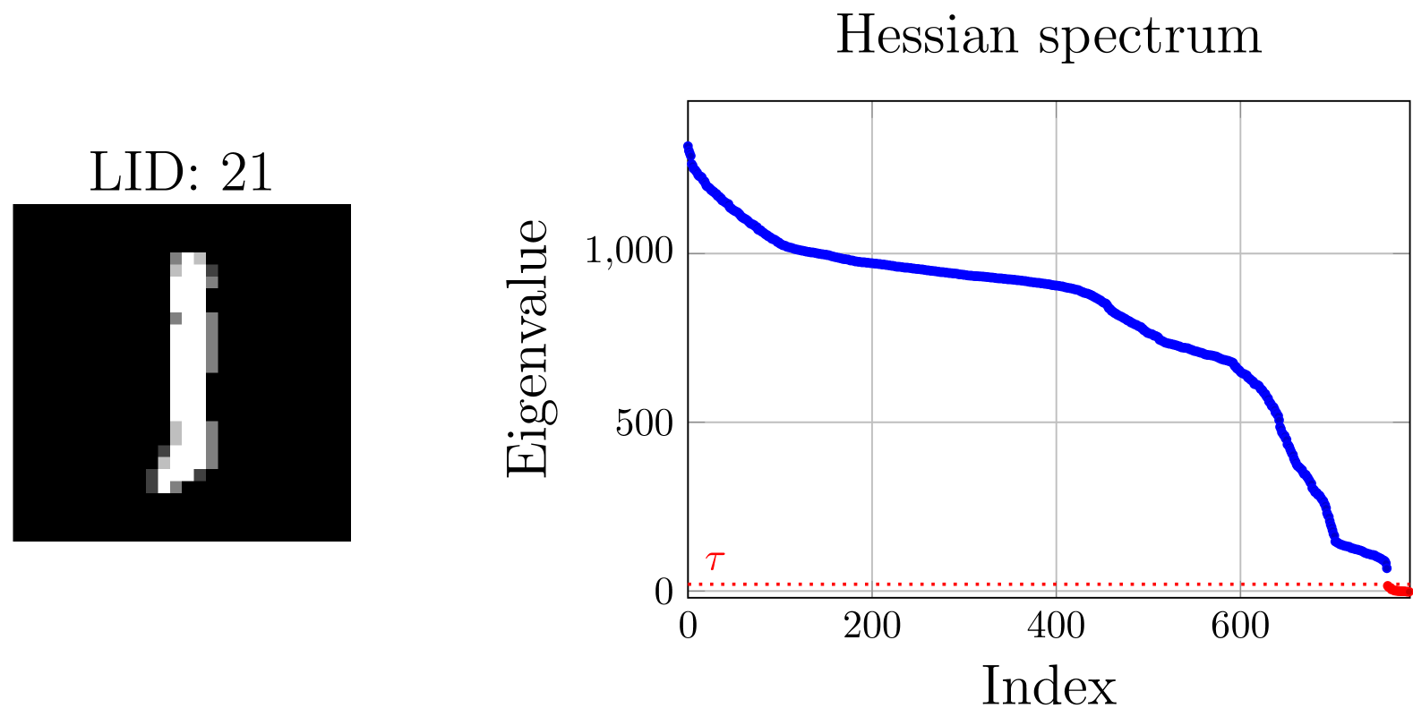
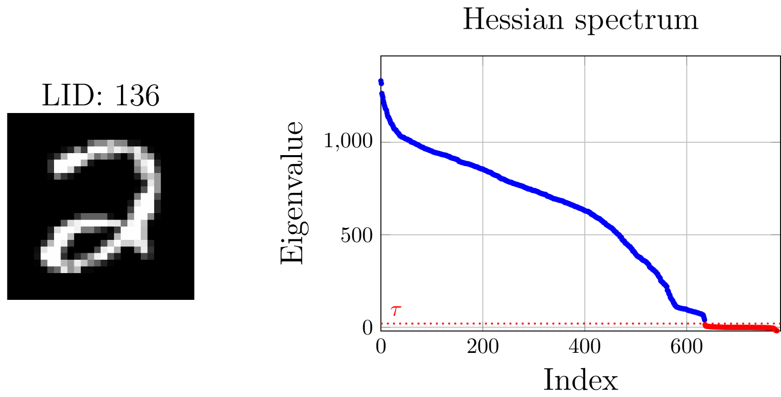
Figure 2: Qualitative results for LID estimation using the Hessian spectrum of $V_{\theta}(x)$. Left: Spectrum for a low-LID image. Right: Spectrum for a high-LID image. The eigenvalues quantify curvature along principal directions (eigenvectors). A degenerate spectrum (many near-zero eigenvalues) indicates locally "flat" regions, revealing the dimension of the local data manifold (LID). Intuitively, higher image complexity often corresponds to a higher LID.

4 Conclusion and limitations

Contributions.

We introduced a generative framework, Energy Matching, that reconciles the advantages of EBMs and OT flow matching models for simulation-free likelihood estimation and efficient high-fidelity generation. Specifically, it:

• Learns a static scalar potential energy whose gradient drives rapid high-fidelity sampling–surpassing state-of-the-art energy based models–while also forming a Boltzmann-like density well suitable for controlled generation. All without auxiliary generators.

• Offers efficient sampling from target data distributions on par with the state-of-the-art, while learning the score at the data manifold with minimal trainable parameters overhead.

• Offers a simulation-free, principled likelihood estimation framework for solving inverse problems—where additional priors can be easily introduced—and enables the estimation of a data point’s LID with fewer approximations than score-based methods.

Limitations.

First, our method requires the extra gradient computation with respect to input, which can increase GPU memory usage (e.g. 20-40%), in particular during training. Second, for very high-resolution datasets, computing the full Hessian spectrum ($O(N^{3})$) may be impractical; and partial spectrum methods like random projections or iterative solvers may be used instead.

Outlook.

In contrast to the widespread belief, we demonstrated that static curl-free methods for generative flows work and offer an exciting direction for future research. Our Energy Matching approach has the potential to yield novel insights into conditional generation and inverse problems for cancer research Weidner et al. (2024); Balcerak et al. (2024), molecules and proteins Wu et al. (2022); Bilodeau et al. (2022), and other fields where precise control over generated samples and effective integration of priors or constraints are crucial.

Appendix A Additional details on Energy Matching

In this section, we provide additional studies and visualizations on our method.

A.1 Energy landscape during training

In Figure˜3, we visualize how the potential $V_{\theta}(x)$ transitions from a flow-like regime, where the OT loss enforces nearly zero curvature away from the data manifold (a), to an EBM-like regime, where the curvature around the new data geometry (here, two moons) is adaptively increased to approximate $\log p_{\text{data}}(x)$ (b). This two-stage design yields a well-shaped landscape that is both efficient to sample (thanks to a mostly flat potential between clusters) and accurate for density estimation near the data modes. For comparison, (c) shows an EBM trained solely with contrastive divergence, exhibiting sharper but less globally consistent basins.

Figure 3: Visualization of the energy $V_{\theta}(x)$ landscapes driving the samples from eight Gaussians to two moons. See Figure˜1 for the 2D perspective. (a) The OT flow loss enforces zero curvature in $V_{\theta}(x)$ along the trajectories to the target. (b) Around the 2 Moons, the curvature of $V_{\theta}(x)$ is adjusted to approximate $\log p_{\text{moons}}(x)\propto V_{\theta}(x)$ while remaining close to the pretrained landscape elsewhere. Combining these objectives yields a potential energy landscape that is both efficient for sampling and representative of the underlying target data distribution. (c) An EBM is shown for comparison, trained using contrastive divergence loss. Visible mode collapse that slows down the equilibration. Less regular landscape away from the data as it needs many simulations to explore it.

A.2 Ablation on the sampling time

Here, we provide ablation studies on CIFAR-10 unconditional generation. Specifically, we first pretrain using $\operatorname{\mathcal{L}_{\mathrm{OT}}}$, and then fine-tune with $(\operatorname{\mathcal{L}_{\mathrm{OT}}}+\operatorname{\mathcal{L}_{\mathrm{CD}}})$. This procedure produces a stable Boltzmann distribution from which one can sample. In the case of $\operatorname{\mathcal{L}_{\mathrm{OT}}}$, the quality measure drops (FID increases) sharply when sampling at $\operatorname{\tau_{s}}>1$. The reason for this is that once the samples move close to the data manifold there is no Boltzmann-like potential well to keep them from drifting away. We report results for different $\operatorname{\tau^{\ast}}$, which influences the sampling along the paths towards the data manifold (see Equation˜3).

Figure 4: CIFAR-10 unconditional generation FID vs. sampling time $\operatorname{\tau_{s}}$ when sampling from models trained under different scenarios: pure $\operatorname{\mathcal{L}_{\mathrm{OT}}}$ and combined $(\operatorname{\mathcal{L}_{\mathrm{OT}}}+\operatorname{\mathcal{L}_{\mathrm{CD}}})$, with temperature regime switching parameter $\operatorname{\tau^{\ast}}\in\{0.9,1.0\}$. Lower FID indicates better generative quality. All results for Euler-Heun with $\Delta t=0.01$.

Appendix B Details on LID estimation

Definition.

To start, we need to introduce the concept of local mass, defined as

$$M(r)\;=\;\int_{B(x_{\text{data}};r)}p(x)\,dx,$$

where $p(x)$ is the local density and $B(x_{\text{data}},r)$ is a ball of radius $r$ around $x_{\text{data}}$, i.e. $B(x_{\text{data}},r)=\{x\in\mathbb{R}^{d}:\|x-x_{\mathrm{data}}\|\leq r\}$. The LID is then given by:

$$\mathrm{LID}(x_{\mathrm{data}})=d-\lim_{r\to 0}\frac{\log\bigl(M(r)\bigr{missing})}{\log(r)}.$$

Intuitively, $M(r)$ measures how much probability mass is concentrated in a ball of radius $r$ around $x_{\mathrm{data}}$. As we shrink this ball, the growth rate of $M(r)$ in terms of $r$ reveals the local dimensional structure of the data.

Assumptions.

In the context of contrastive divergence, we assume that data points $x_{\mathrm{data}}$ lie in well-like regions [Hyvärinen, 2006], i.e.:

$$\nabla V(x_{\mathrm{data}})\approx 0\quad\text{and}\quad\nabla^{2}V(x_{\mathrm{data}})\text{ is positive semidefinite (or nearly so).}$$

Conceptually, $V(x)$ can be thought of as an energy function; points where $\nabla V(x_{\mathrm{data}})=0$ are near local minima of this energy, and the Hessian $\nabla^{2}V(x_{\mathrm{data}})$ provides information about local curvature (see Figure˜2 for a qualitative illustration).

Energy-based density.

We define an energy-based density

$$p(x)\;\propto\;\exp\!\Bigl{(}-\tfrac{V(x)}{\varepsilon}\Bigr{)},$$

where $\varepsilon$ is a temperature parameter. Near a data point $x_{\mathrm{data}}$ satisfying $\nabla_{x}V(x_{\mathrm{data}})=0$, we can approximate $V(x)$ by its second-order Taylor expansion:

$$V(x)\approx V(x_{\mathrm{data}})+\frac{1}{2}(x-x_{\mathrm{data}})^{\top}\nabla_{x}^{2}V(x_{\mathrm{data}})(x-x_{\mathrm{data}}).$$

Consequently, in view of the assumptions above,

$$p(x)\propto\exp\left(-\frac{1}{2\varepsilon}(x-x_{\mathrm{data}})^{\top}\nabla_{x}^{2}V(x_{\mathrm{data}})(x-x_{\mathrm{data}})\right).$$

Local mass derivation and the rank of the energy Hessian.

Substituting the local quadratic form of $p(x)$ near $x_{\mathrm{data}}$ into the definition of the local mass $M(r)$, we obtain:

$$M(r)=\int_{B(x_{\text{data}},r)}p(x)dx\propto\int_{B(x_{\text{data}},r)}\exp\left(-\tfrac{1}{2\varepsilon}(x-x_{\mathrm{data}})^{\top}\nabla_{x}^{2}V(x_{\mathrm{data}})(x-x_{\mathrm{data}})\right)dx.$$

For small $r$, the dominant contribution depends on the rank of the Hessian $\nabla_{x}^{2}V(x_{\mathrm{data}})$. Let $k=\mathrm{rank}(\nabla_{x}^{2}V(x_{\mathrm{data}}))$. Then, as $r\to 0$, one can show that $M(r)=Cr^{k}$, where $C$ does not depend on $r$. We take the logarithm on both sides and divide by $\log(r)$ to get

$$\frac{\log(M(r))}{\log(r)}=\frac{\log(C)+k\log(r)}{\log(r)}=k+\frac{\log(C)}{\log(r)},$$

and the second term vanishes as $r\to 0$. Hence,

$$\mathrm{LID}(x_{\mathrm{data}})=d-k.$$

Practical estimation.

In practice, the LID at a data point $x_{\mathrm{data}}$ can be estimated through the following procedure:

1. Train $V(x)$ with Energy Matching.

2. Compute the Hessian $H=\nabla_{x}^{2}V(x_{\mathrm{data}})$.

3. Perform an eigenvalue decomposition on $H$.

Then the estimated local data-manifold dimension corresponds to the number of directions with negligible curvature (smaller magnitude than some $\tau$).

Appendix C Training Details

Below, we detail the training configurations for CIFAR-10, CelebA, and MNIST. The gradient of the potential, $\nabla_{x}V(x)$, is computed using automatic differentiation via PyTorch’s autograd.

CIFAR-10.

The architecture is shown in Figure˜5. We use the same UNet from [Tong et al., 2023] (with fixed $t=0.0$, making it effectively static) followed by a small vision transformer (ViT) [Dosovitskiy et al., 2020] to obtain a scalar output. Hyperparameters are: $\tau_{s}=3.0$, $\tau^{*}=0.9$, $\Delta t=0.01$, $M_{\text{Langevin}}=200$. We train for 200k iterations using Algorithm˜1 and then 25k more with Algorithm˜2 on 4xA100. The batch size is 128, learning rate is $8\times 10^{-4}$, $\varepsilon_{\max}=0.01$, and $\lambda_{\mathrm{CD}}=2\times 10^{-4}.$

CelebA.

We scale the CIFAR-10 model by $\sim 2\times$; see Figure˜6. We keep $\tau_{s}=3.0$, $\tau^{*}=0.9$, $\Delta t=0.01$, $M_{\text{Langevin}}=200$, and train for 250k iterations using Algorithm˜1 then 25k with Algorithm˜2 on 4xA100. The batch size is 32, learning rate is $1\times 10^{-4}$, $\varepsilon_{\max}=0.05$, and $\lambda_{\mathrm{CD}}=2\times 10^{-5}$.

MNIST.

We train on a single RTX6000 directly with Algorithm˜2 for 300k iterations using $\lambda_{\mathrm{CD}}=0.25$, $\Delta t=0.05$, and $M_{\text{Langevin}}=50$. The architecture consists of a two-stage CNN followed by a two-layer MLP, comprising a total of 2M parameters.

Hyperparameter	Value
Image size	3$\times$32$\times$32
Base channels (UNet)	128
ResBlocks	2
channel_mult	[1, 2, 2, 2]
Attention resolution	16
Attention heads (UNet)	4
Head channels (UNet)	64
Dropout	0.1
Transformer (ViT) Head
Patch size	4
Embedding dim	384
Transformer layers	8
Transformer heads	4
Output scale	1000.0

Figure 5: Diagram of our UNet+Transformer EBM for CIFAR-10. A UNet (37M params) processes a 3$\times$32$\times$32 image; its output is fed into a Transformer head (PatchEmbed + 8-layer ViT, 12M params) that produces a scalar potential. Here we employ the identical UNet architecture as in [Tong et al., 2023].

Hyperparameter	Value
Image size	3$\times$64$\times$64
Base channels (UNet)	128
ResBlocks	2
channel_mult	[1, 2, 3, 4]
Attention resolution	16
Attention heads (UNet)	4
Head channels (UNet)	64
Dropout	0.1
Transformer (ViT) Head
Patch size	4
Embedding dim	512
Transformer layers	8
Transformer heads	8
Output scale	1000.0

Figure 6: Diagram of our UNet+Transformer EBM for CelebA. A UNet (83M params) processes a 3$\times$64$\times$64 image; its output is fed into a Transformer head (PatchEmbed+8-layer ViT, 25M params) that produces a scalar potential.

References

- Ambrosio et al. [2008] L. Ambrosio, N. Gigli, and G. Savaré. Gradient flows: in metric spaces and in the space of probability measures. 2008.
- Balcerak et al. [2024] Michal Balcerak, Tamaz Amiranashvili, Andreas Wagner, Jonas Weidner, Petr Karnakov, Johannes C Paetzold, Ivan Ezhov, Petros Koumoutsakos, Benedikt Wiestler, et al. Physics-regularized multi-modal image assimilation for brain tumor localization. Advances in Neural Information Processing Systems, 37:41909–41933, 2024.
- Ben-Hamu et al. [2024] Heli Ben-Hamu, Omri Puny, Itai Gat, Brian Karrer, Uriel Singer, and Yaron Lipman. D-flow: differentiating through flows for controlled generation. In Proceedings of the 41st International Conference on Machine Learning, pages 3462–3483, 2024.
- Bilodeau et al. [2022] Camille Bilodeau, Wengong Jin, Tommi Jaakkola, Regina Barzilay, and Klavs F Jensen. Generative models for molecular discovery: Recent advances and challenges. Wiley Interdisciplinary Reviews: Computational Molecular Science, 12(5):e1608, 2022.
- Butcher [2016] John C. Butcher. Numerical Methods for Ordinary Differential Equations. John Wiley & Sons, 3rd edition, 2016.
- Choi et al. [2024] Jaemoo Choi, Jaewoong Choi, and Myungjoo Kang. Scalable wasserstein gradient flow for generative modeling through unbalanced optimal transport. In International Conference on Machine Learning, pages 8629–8650. PMLR, 2024.
- Chung et al. [2023] Hyungjin Chung, Jeongsol Kim, Michael T Mccann, Marc L Klasky, and Jong Chul Ye. Diffusion posterior sampling for general noisy inverse problems. In The Eleventh International Conference on Learning Representations, 2023.
- Cui and Han [2024] Jiali Cui and Tian Han. Learning latent space hierarchical ebm diffusion models. In Proceedings of the 41st International Conference on Machine Learning, pages 9633–9645, 2024.
- Daras et al. [2024] Giannis Daras, Hyungjin Chung, Chieh-Hsin Lai, Yuki Mitsufuji, Jong Chul Ye, Peyman Milanfar, Alexandros G Dimakis, and Mauricio Delbracio. A survey on diffusion models for inverse problems. arXiv preprint arXiv:2410.00083, 2024.
- Deng [2012] Li Deng. The mnist database of handwritten digit images for machine learning research. IEEE Signal Processing Magazine, 29(6):141–142, 2012.
- Dosovitskiy et al. [2020] Alexey Dosovitskiy, Lucas Beyer, Alexander Kolesnikov, Dirk Weissenborn, Xiaohua Zhai, Thomas Unterthiner, Mostafa Dehghani, Matthias Minderer, G Heigold, S Gelly, et al. An image is worth 16x16 words: Transformers for image recognition at scale. In International Conference on Learning Representations, 2020.
- Du and Mordatch [2019] Yilun Du and Igor Mordatch. Implicit generation and modeling with energy based models. Advances in Neural Information Processing Systems, 32, 2019.
- Du et al. [2021] Yilun Du, Shuang Li, Joshua Tenenbaum, and Igor Mordatch. Improved contrastive divergence training of energy-based models. In International Conference on Machine Learning, pages 2837–2848. PMLR, 2021.
- Fefferman et al. [2016] Charles Fefferman, Sanjoy Mitter, and Hariharan Narayanan. Testing the manifold hypothesis. Journal of the American Mathematical Society, 29(4):983–1049, 2016.
- Flamary et al. [2021] Rémi Flamary, Nicolas Courty, Alexandre Gramfort, Mokhtar Z Alaya, Aurélie Boisbunon, Stanislas Chambon, Laetitia Chapel, Adrien Corenflos, Kilian Fatras, Nemo Fournier, Léo Gautheron, Nathalie T H Gayraud, Hicham Janati, Alain Rakotomamonjy, Ievgen Redko, Antoine Rolet, Antony Schutz, Vivien Seguy, Danica J Sutherland, Romain Tavenard, Alexander Tong, and Titouan Vayer. POT: Python Optimal Transport. Journal of Machine Learning Research, 22(78):1–8, 2021.
- Gao et al. [2021] Ruiqi Gao, Yang Song, Ben Poole, Ying Nian Wu, and Diederik P Kingma. Learning energy-based models by diffusion recovery likelihood. In International Conference on Learning Representations, 2021.
- Guo et al. [2023] Qiushan Guo, Chuofan Ma, Yi Jiang, Zehuan Yuan, Yizhou Yu, and Ping Luo. Egc: Image generation and classification via a diffusion energy-based model. In 2023 IEEE/CVF International Conference on Computer Vision (ICCV), pages 22895–22905. IEEE Computer Society, 2023.
- Hinton [2002] Geoffrey E Hinton. Training products of experts by minimizing contrastive divergence. Neural computation, 14(8):1771–1800, 2002.
- Ho et al. [2020] Jonathan Ho, Ajay Jain, and Pieter Abbeel. Denoising diffusion probabilistic models. Advances in neural information processing systems, 33:6840–6851, 2020.
- Hopfield [1982] J. J. Hopfield. Neural networks and physical systems with emergent collective computational abilities. Proceedings of the National Academy of Sciences, 79(8):2554–2558, 1982.
- Hyvärinen [2006] Aapo Hyvärinen. Connections between score matching, contrastive divergence, and pseudolikelihood for continuous-valued data. Neural Computation, 18(8):1527–1550, 2006.
- Johnsson et al. [2014] Kerstin Johnsson, Charlotte Soneson, and Magnus Fontes. Low bias local intrinsic dimension estimation from expected simplex skewness. IEEE transactions on pattern analysis and machine intelligence, 37(1):196–202, 2014.
- Jordan et al. [1998] Richard Jordan, David Kinderlehrer, and Felix Otto. The variational formulation of the fokker–planck equation. SIAM Journal on Mathematical Analysis, 29(1):1–17, 1998.
- Kamkari et al. [2024] Hamid Kamkari, Brendan Ross, Rasa Hosseinzadeh, Jesse Cresswell, and Gabriel Loaiza-Ganem. A geometric view of data complexity: Efficient local intrinsic dimension estimation with diffusion models. Advances in Neural Information Processing Systems, 37:38307–38354, 2024.
- Lanzetti et al. [2024] Nicolas Lanzetti, Antonio Terpin, and Florian Dörfler. Variational analysis in the wasserstein space. arXiv preprint arXiv:2406.10676, 2024.
- Lanzetti et al. [2025] Nicolas Lanzetti, Saverio Bolognani, and Florian Dörfler. First-order conditions for optimization in the wasserstein space. SIAM Journal on Mathematics of Data Science, 7(1):274–300, 2025.
- LeCun et al. [2006] Yann LeCun, Sumit Chopra, Raia Hadsell, M Ranzato, and F Huang. A tutorial on energy-based learning. Predicting Structured Data, 1(0), 2006.
- Lee et al. [2023] Hankook Lee, Jongheon Jeong, Sejun Park, and Jinwoo Shin. Guiding energy-based models via contrastive latent variables. arXiv preprint arXiv:2303.03023, 2023.
- Lipman et al. [2023] Yaron Lipman, Ricky TQ Chen, Heli Ben-Hamu, Maximilian Nickel, and Matthew Le. Flow matching for generative modeling. In ICLR, 2023.
- Liu et al. [2023] Xingchao Liu, Chengyue Gong, et al. Flow straight and fast: Learning to generate and transfer data with rectified flow. In The Eleventh International Conference on Learning Representations, 2023.
- Liu et al. [2015] Ziwei Liu, Ping Luo, Xiaogang Wang, and Xiaoou Tang. Deep learning face attributes in the wild. In Proceedings of International Conference on Computer Vision (ICCV), December 2015.
- Mardani et al. [2024] Morteza Mardani, Jiaming Song, Jan Kautz, and Arash Vahdat. A variational perspective on solving inverse problems with diffusion models. ICLR, 2024.
- Neklyudov et al. [2023] Kirill Neklyudov, Rob Brekelmans, Daniel Severo, and Alireza Makhzani. Action matching: Learning stochastic dynamics from samples. In Proceedings of the 40th International Conference on Machine Learning, volume 202 of Proceedings of Machine Learning Research, pages 25858–25889. PMLR, 23–29 Jul 2023.
- Song and Ermon [2019] Yang Song and Stefano Ermon. Generative modeling by estimating gradients of the data distribution. Advances in neural information processing systems, 32, 2019.
- Song and Kingma [2021] Yang Song and Diederik P Kingma. How to train your energy-based models. arXiv preprint arXiv:2101.03288, 2021.
- Song et al. [2021] Yang Song, Jascha Sohl-Dickstein, Diederik P. Kingma, Abhishek Kumar, Stefano Ermon, and Ben Poole. Score-based generative modeling through stochastic differential equations. In International Conference on Learning Representations, 2021.
- Stanczuk et al. [2024] Jan Pawel Stanczuk, Georgios Batzolis, Teo Deveney, and Carola-Bibiane Schönlieb. Diffusion models encode the intrinsic dimension of data manifolds. In Forty-first International Conference on Machine Learning, 2024.
- Sun et al. [2025] Qiao Sun, Zhicheng Jiang, Hanhong Zhao, and Kaiming He. Is noise conditioning necessary for denoising generative models? arXiv preprint arXiv:2502.13129, 2025.
- Terpin et al. [2024] Antonio Terpin, Nicolas Lanzetti, Martín Gadea, and Florian Dorfler. Learning diffusion at lightspeed. Advances in Neural Information Processing Systems, 37:6797–6832, 2024.
- Tong et al. [2023] Alexander Tong, Kilian FATRAS, Nikolay Malkin, Guillaume Huguet, Yanlei Zhang, Jarrid Rector-Brooks, Guy Wolf, and Yoshua Bengio. Improving and generalizing flow-based generative models with minibatch optimal transport. Transactions on Machine Learning Research, 2023.
- Vapnik [1995] Vladimir N. Vapnik. The Nature of Statistical Learning Theory. Springer-Verlag, 1995.
- Weidner et al. [2024] Jonas Weidner, Ivan Ezhov, Michal Balcerak, Marie-Christin Metz, Sergey Litvinov, Sebastian Kaltenbach, Leonhard Feiner, Laurin Lux, Florian Kofler, Jana Lipkova, et al. A learnable prior improves inverse tumor growth modeling. IEEE Transactions on Medical Imaging, 2024.
- Welling and Teh [2011] Max Welling and Yee W Teh. Bayesian learning via stochastic gradient langevin dynamics. In Proceedings of the 28th international conference on machine learning (ICML-11), pages 681–688. Citeseer, 2011.
- Wu et al. [2022] Lemeng Wu, Chengyue Gong, Xingchao Liu, Mao Ye, and Qiang Liu. Diffusion-based molecule generation with informative prior bridges. Advances in neural information processing systems, 35:36533–36545, 2022.
- Xu et al. [2023] Chen Xu, Xiuyuan Cheng, and Yao Xie. Normalizing flow neural networks by jko scheme. Advances in Neural Information Processing Systems, 36, 2023.
- Zhang et al. [2024] Yasi Zhang, Peiyu Yu, Yaxuan Zhu, Yingshan Chang, Feng Gao, Ying Nian Wu, and Oscar Leong. Flow priors for linear inverse problems via iterative corrupted trajectory matching. arXiv preprint arXiv:2405.18816, 2024.
- Zhu et al. [2024] Yaxuan Zhu, Jianwen Xie, Ying Nian Wu, and Ruiqi Gao. Learning energy-based models by cooperative diffusion recovery likelihood. In The Twelfth International Conference on Learning Representations, 2024.