Simulating near-infrared spectroscopy on a quantum computer for enhanced chemical detection

Abstract

Near-infrared (NIR) spectroscopy is a non-invasive, low-cost, reagent-less, and rapid technique to measure chemical concentrations in a wide variety of sample types. However, extracting concentration information from the NIR spectrum requires training a statistical model on a large collection of measurements, which can be impractical, expensive, or dangerous. In this work, we propose a method for simulating NIR spectra on a quantum computer, as part of a larger workflow to improve NIR-based chemical detection. The quantum algorithm is highly optimized, exhibiting a cost reduction of many orders of magnitude relative to prior approaches. The main optimizations include the localization of vibrational modes, an efficient real-space-based representation of the Hamiltonian with a quantum arithmetic-based implementation of the time-evolution, optimal Trotter step size determination, and specific targeting of the NIR region. Overall, our algorithm achieves a $\mathcal{O}(M^{2})$ scaling, compared with the $\mathcal{O}(M^{12})$ coming from equivalent high-accuracy classical methods. As a concrete application, we show that simulating the spectrum of azidoacetylene (HC${}_{2}$N${}_{3}$), a highly explosive molecule with strong anharmonicities consisting of $M=12$ vibrational modes, requires circuits with a maximum $8.47\times 10^{8}$ T gates and $173$ logical qubits. By enhancing the training datasets of detection models, the full potential of vibrational spectroscopy for chemical detection could be unlocked across a range of applications, including pharmaceuticals, agriculture, environmental monitoring, and medical sensing.

I Introduction

Detection of harmful chemicals in the air, water and soil is a crucial first step to tackling environmental and industrial pollution [slonecker2010visible, wilson2012review, tan2019scheme, thakur2022recent]. Near-infrared absorption spectroscopy (NIRS) is particularly well-suited to this task [huck2006near, sulub2007spectral, siesler2008near, ozaki2018near, bik2020lipid, bec2022silico]: it is a non-destructive, ultrafast, reagent-less, easily miniaturized technique with broad applicability across different media, with no sample preparation requirements. Wide adoption of NIRS for tracking harmful chemicals could deliver real-time spatiotemporal data essential for addressing challenges as diverse as disaster relief [jha2008advances], disease diagnosis [adegoke2021near], agricultural soil quality monitoring [cecillon2009assessment], medical sensing [medical], and climate change [counsell2016recent, corradini2019predicting, zhao2023role].

While the near-infreared (NIR) spectrum is rich in chemical-identifying information, this information is nontrivial to extract [sulub2007spectral, palafox2017computational, bec2019breakthrough, ozaki2021near]. The NIR region of $12,500-4,000$ cm${}^{-1}$ ($800-2,500$ nm) is dominated by combination and overtone vibrational bands. These bands often include large anharmonic effects that make band assignment from harmonic frequencies virtually impossible. In addition, the combinatorial number of bands yields broad distributions of intensities across many wavelengths. Spectral fingerprinting in this NIR region thus requires to go beyond peak identification and incorporate information from the entire spectrum. It is thus necessary to collect a large amount of spectral and concentration data, and then use it to train statistical models to correlate certain global spectral patterns with chemical concentration [beebe1998chemometrics, ozaki2021near]. Such data collection is often time-consuming [nagy2022quality], expensive [grabska2017temperature, sibert2023modeling], and even dangerous [tan2019scheme, van2023rapid], depending on the chemical of interest.

Simulating NIR spectra is a promising way to augment NIR training datasets [westad2008incorporating, bec2018nir, bec2019simulated, ozaki2021advances]. It is inherently safe, inexpensive, and has the potential to alleviate many of the challenges associated with collecting training data. However, while fundamental frequencies appearing in the mid-IR region ($4,000-400$ cm${}^{-1}$) can be simulated with sufficient accuracy by inexpensive methods like harmonic analysis [bec2021introduction], the presence of combination and overtone bands in NIR necessitates the use of much more computationally demanding techniques such as vibrational configuration interaction (VCI) [ozaki2021advances, oschetzki2013azidoacetylene]. While VCI and similar approaches are capable of accurately predicting peak positions and intensities of such bands, the associated runtime and memory cost scales prohibitively with system size, motivating the need for alternative approaches. This steep cost scaling has thus far restricted the applicability of NIR simulations to industrially useful contexts [bec2021introduction].

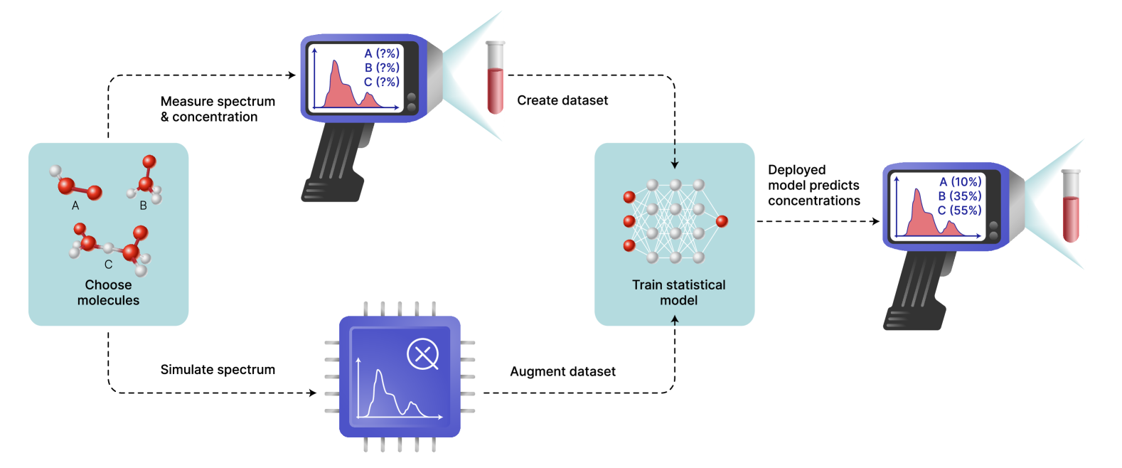
Figure 1: Chemical detection using near-infrared absorption spectra. Once a molecule is chosen, one typically needs to collect many measurements of varying concentrations and under different conditions in order to train a statistical model that can then infer the concentration of the molecule by detecting a signature of its spectrum in an unknown sample. We propose augmenting the training dataset and training process of the statistical model using simulated NIR spectra obtained on a quantum computer.

In contrast to the steep scaling from high-accuracy classical solutions, the usage of quantum computers presents a promising avenue for escalating calculations to larger systems. However, previous estimates for the cost of quantum-based simulation of vibrational systems were beyond the reach of early fault-tolerant hardware [ibm_vibrational], motivating the need for more efficient quantum algorithms. In this work, we propose a novel quantum algorithm for simulating vibrational spectra of molecules. The algorithm is shown to deliver high-accuracy NIR spectra at significantly more affordable computational cost and favourable scaling compared to classical approaches of similar accuracy. The algorithm is highly optimized to decrease constant factors in the runtime, achieving a reduction of many orders of magnitude compared with earlier quantum methods [ibm_vibrational], and already becoming competitive in runtime with state-of-the-art classical techniques for modestly-sized molecules with only seven to ten atoms.

The optimizations used in the algorithm consist of the following: mode localization techniques for reducing the required number of terms in the Hamiltonian while achieving high-accuracy [mode_loc_1, mode_loc_2, mode_loc_3, mode_loc_4], a real-space representation of the vibrational Hamiltonian [macridin_1, macridin_2], alongside its associated quantum-arithmetic-based implementation of the Trotterized time-evolution operator (adapted from the vibronic algorithm in Ref. [vibronic]), a novel and accurate estimation of the Trotter step size based on the perturbative approach from Refs. [trotter_pt, trotter_pt_2], a time-domain quantum algorithm [qpe_gqpe] with a few compilation-based optimizations to reduce its overall cost [new_xas], an optimal window selection plus initial state preparation targeting the NIR region, and usage of the active volume compilation technique [active_volume]. The overall improvements from these optimizations are summarized in Table˜1 for the example of the azidoacetylene HC${}_{2}$N${}_{3}$ molecule.

Optimization technique	Additional qubits	Total qubits	Approximate improvement	Cumulative improvement
1 - Mode localization	$0$	$49$	$\times 50$	$5\times 10^{1}$
2 - Real-space representation	$124$	$173$	$\times 8$	$4\times 10^{2}$
3 - Coefficient caching	$0$	$173$	$\times 2$	$8\times 10^{2}$
4 - Trotter perturbative step	$0$	$173$	$\times 2$	$1.6\times 10^{3}$
5 - Double measurement trick	$0$	$173$	$\times 1.5$	$2.4\times 10^{3}$
6 - Double phase trick	$0$	$173$	$\times 2$	$4.8\times 10^{3}$
7 - Initial state projection	$0$	$173$	$\times 1000$	$4.8\times 10^{6}$
8 - Active volume compilation	$327-1827$	$500-2000$	$\times 25-\times 100$	$1.2\times 10^{8}-4.8\times 10^{8}$

Table 1: List of optimizations with associated estimated improvement ratio to the total runtime required to simulate NIR spectra. The cumulative improvement column corresponds to an aggregate of all optimizations on top of the associated row, while total qubits corresponds to the associated number of qubits. Numbers shown are obtained for the azidoacetylene HC${}_{2}$N${}_{3}$ molecule with $12$ vibrational modes; some optimizations will have a larger improvement for bigger molecules. The mode localization improvement was calculated through the change of number of terms in the Hamiltonian obtained with a $2$-mode expansion instead of $3$-mode. The real-space representation improvement was calculated with respect to the second-quantized modal-based representation of the Hamiltonian [christiansen, ibm_vibrational]. The Trotter step improvement was calculated with respect to the usage of the commutator-based bounds [trotter_error]. Two different budgets of 500 and 2000 logical qubits were considered with the active volume compilation technique to showcase the different improvements.

This paper is organized as follows. In Section˜II, we describe how NIRS is used in practice for chemical detection, highlight the potential benefit of simulations, and elaborate on the challenges faced by existing simulation methods, classical and quantum. We then present the new algorithm in Section˜III, where we lay out all the optimizations that allow us to achieve the large runtime reduction. The algorithm is then benchmarked through proof-of-concept simulations in LABEL:sec:benchmark – simulations which also allow us to perform robust and careful constant-factor resource estimation. Our conclusions are presented in LABEL:sec:conclusions.

II Near-infrared spectroscopy for chemical detection

II.1 Practical spectral fingerprinting with NIRS

When NIR radiation is passed through a sample, it is partially absorbed by the constituent molecules. NIR radiation is energetically too weak to generate electronic excitations, as happens for example with UV-visible or X-ray spectroscopy: instead, incoming radiation is translated into vibrations of the atoms in the absorbing molecule. The key quantity measured in NIRS experiments is the absorption cross-section $\sigma_{A}(\omega)$, a function indicating the strength of absorption at a particular frequency of incoming radiation $\omega$. Within the dipole approximation, it is given by

$$\sigma_{A}(\omega)\propto\omega\sum_{\rho=x,y,z}\sum_{f}|\langle E_{f}\rvert\hat{\mu}_{\rho}\lvert E_{0}\rangle|^{2}\mathcal{L}_{\eta}(\omega-E_{f}+E_{0}).$$ (1)

Here $\lvert E_{0}\rangle,\lvert E_{f}\rangle$ are the ground and excited states of a molecular vibrational Hamiltonian $\hat{H}$, $\omega$ is the frequency of incoming radiation, $\hat{\mu}_{\rho}$ is the $\rho$-th Cartesian component of the molecular dipole operator, and $\mathcal{L}_{\eta}(\omega)=\eta/(\omega^{2}+\eta^{2})$ is the Lorentzian broadening with $\eta$ its half-width at half-maximum. This broadening is related to the lifetime of excited states of the system as well as the resolution of the measurement apparatus, and in practice usually takes values between $\eta=1$ cm${}^{-1}$ and $10$ cm${}^{-1}$.

The set of peak positions $E_{f}$ and absorption intensities $|\langle E_{f}\rvert\hat{\mu}_{\rho}\lvert E_{0}\rangle|^{2}$ is unique to a given molecule, being determined by the details of its ground-state potential energy surface (PES). Since peaks and their intensities completely determine the absorption spectrum, that implies the spectrum itself is a unique fingerprint of the molecule. Thus if molecular spectra are cataloged a priori, it should be possible to detect the presence of a given molecule in an unknown sample through a direct comparison against the catalog. This is indeed how chemical detection occurs with mid-IR spectra. The peaks present in the mid-IR range ($4,000-400$ cm${}^{-1}$) are fundamental vibrational excitations: there is usually no shortage of sharp, high-intensity features that are highly specific to a given molecule and thus can serve as good spectral fingerprints [haas2016advances].

However, near-IR spectroscopy has many advantages as an experimental technique, advantages that often make it more desirable than mid-IR for detection applications [huck2006near, bec2022silico]. In addition to being a low-cost and high-speed approach, weaker absorption means that it can be applied to much larger samples, as it is able to penetrate into the bulk; for the same reason, NIRS is applicable to a much wider variety of phases of matter [siesler2008near, bik2020lipid]. At the same time, the ease of miniaturization of devices operating in the NIR part of the spectrum allows for truly portable detectors [alcala2013qualitative, wiedemair2018application, adegoke2021near] – most recently even reaching an individual consumer though cheap mobile phone attachments [klakegg2016instrumenting, watanabe2016development, huang2021applications]. On the instrumentation side, the telecommunications industry has commercialized many of the technologies that enabled cheap and reliable NIRS – chiefly among those the ability to use fiber optic cables for optic light transmission [martin2002near], an approach off-limits to mid-IR due to high signal attenuation in fiber optic in the associated spectral region. Finally, since very little or no sample preparation is required during spectrum acquisition [ozaki2018near, sulub2007spectral], the method is uniquely non-destructive and non-invasive.

All these advantages make NIRS a desirable approach for chemical detection. Unfortunately, unlike their mid-IR counterparts, NIR spectra typically feature broad distributions of intensity spread across many wavelengths, rather than sharp isolated features that would make it easy to identify specific molecules by a handful of key wavelengths. While the spectra are still unique to a given molecule, a correct identification requires taking into account the global intensity pattern rather than a few isolated signature peaks [sulub2007spectral, palafox2017computational, bec2019breakthrough, ozaki2021near].

What this means in practice is that identification via direct comparison to stored spectra is no longer possible. Instead, it becomes necessary to train a statistical model to detect a given molecule using its spectrum. A typical workflow for NIR-based chemical detection consists of the steps shown in Fig.˜1 without the quantum simulation of the spectrum and associated dataset augmentation. Training statistical models requires large amounts of data to achieve high accuracy and transferability between measurement apparatuses and experimental contexts. Collecting a sufficient amount of data for model training is often expensive or otherwise challenging. This could be due to working with dangerous chemicals (e.g. toxic [tan2019scheme] or explosive [van2023rapid]), the conformers being hard to separate in the laboratory [grabska2017temperature, sibert2023modeling], or simply due to the large amount of data needed in the first place, for example when working with natural products [nagy2022quality].

Simulations of NIR spectra [bec2021current, barone2021computational, ozaki2021advances], a source of “synthetic data”, may help address these limitations [westad2008incorporating, bec2018nir, bec2019simulated, ozaki2021advances]. First, augmenting experimental datasets with simulated data could significantly alleviate the costs associated with data acquisition, and speed up the deployment process. Simulated data are also inherently safe to procure, removing any security concerns. Second, simulations provide additional information above and beyond the spectrum itself, for instance access to the underlying states and their symmetries, ability to vary geometry, environment effects, and so on. This information may be used to improve the sensitivity and specificity of statistical models, for example by selecting the key wavelengths most correlated with the property of interest on physical grounds, rather than purely statistically. And finally, this same information may also be used to aid in interpreting the results of a statistical model, building spectrum-structure relationships, thus enhancing reliability, trust, and transferability of the model [westad2008incorporating, bec2018nir, bec2022silico].

II.2 Classical simulation of NIRS

Unlike in electronic structure, computational chemistry simulations methods for vibrational problems have received comparatively less attention. Most of the techniques from the former have found their counterparts in the latter: starting with the mean-field-like vibrational self-consistent field (VSCF) [vscf_1, vscf_2, vscf_3, vscf_4], and continuing up the accuracy and complexity scale to standard vibrational perturbation theory (VPT) [nielsen1951vibration, clabo1988systematic, lutz2014reproducible] and its many variants such as deperturbed and generalized flavours [barone2005anharmonic, bloino2016aiming, krasnoshchekov2015ab, grabska2018nir], vibrational coupled cluster (VCC) [christiansen, christiansen2004vibrational, seidler2009automatic, seidler2011vibrational, faucheaux2015higher, hansen2020extended], the already mentioned vibrational configuration interaction (VCI) [fujisaki2007quantum, seidler2010vibrational, oschetzki2013azidoacetylene, schroder2022vibrational], as well as the very recently introduced vibrational density-matrix renormalization group (vDMRG) [baiardi2017vibrational, glaser2023flexible] and various selective or adaptive vibrational configuration interaction approaches [scribano2008iterative, neff2009toward, fetherolf2021vibrational, schroder2021incremental].

In practice, the VSCF approach is mostly helpful for molecules with weak anharmonicities in the PES, and is rarely used by itself in the strongly anharmonic NIR region [roy2013vibrational, lutz2014reproducible, ozaki2021advances]. However, much like its Hartree-Fock counterpart, it serves as a starting point for all the higher-complexity methods, being a source of high-quality single-mode basis wavefunctions (called modals) – linear combinations of canonical harmonic oscillator modes that best capture anharmonicity effects in a mean-field way.

The VCC and VCI approaches with a sufficiently high allowed excitation order (typically at least quadruple, e.g. VCI-SDTQ), can usually provide the accuracy needed in chemical detection applications, yielding spectra that match well to experiment [oschetzki2013azidoacetylene, samsonyuk2013configuration, ozaki2021advances]. However, their prohibitive cost generally precludes their application to molecules with more than a dozen atoms, leading to them not being very widely used in practice. Vibrational perturbation theory is a middle ground, combining relative speed of execution with reasonable accuracy. But the technique is far from universal, requiring fine-tuning as it suffers from near-degeneracies (leading to the proliferation of approaches to tackling those [barone2005anharmonic, bloino2016aiming, krasnoshchekov2015ab, grabska2018nir]), which become only more commonplace with increasing system size. While several methods have been developed to isolate and tackle such degeneracies, there are still numerous examples of where the VPT-produced spectrum differs significantly from the experimental one [bec2018spectra, piccardo2015generalized, krasnoshchekov2015nonempirical, grabska2021theoretical].

Finally, for completeness we mention here the very recently introduced vDMRG [baiardi2017vibrational, glaser2023flexible] and selective VCI [scribano2008iterative, neff2009toward, fetherolf2021vibrational, schroder2021incremental] approaches. They have shown a lot of promise, especially when it comes to the mid-IR: however, these methods are yet to be tested more broadly, especially in the strongly-anharmonic NIR region. While the electronic counterparts of vDMRG and selective VCI are state-of-the-art for predicting electronic ground-state properties, they continue to face challenges when it comes to computing spectra: this manifests as limitations in terms of achievable system sizes. These tend to be especially severe for highly-excited states – exactly the ones making up the NIR spectrum.

Limitations of existing methods have motivated a few researchers to consider quantum approaches. This has led to intriguing arguments for why quantum advantage might manifest sooner in the vibrational structure problem rather than in electronic structure [sawaya2021near]. There has also been prior work estimating the cost of computing vibrational spectra on fault-tolerant hardware, done on the example of a series of polymers of increasing size [ibm_vibrational]. However, this resource estimate was very high, casting doubt on whether a quantum approach to vibrational problems would be worthwhile. We also note that an approach has been proposed for using the variational quantum eigensolver for the ground-state vibrational problem [vqe_vib]. However, besides the convergence problems outlined in that work, it does not seem likely that the variational quantum eigensolver can be efficiently used for the spectroscopic problem where a large collection of excited states is required.

Motivated by this inability of existing classical to provide affordable high-quality training data for NIR-based chemical detection, in the rest of this paper we lay out a highly-optimized quantum algorithm for computing vibrational spectra of molecules. LABEL:app:scaling shows a deduction of the scaling of both our algorithm and VCI-SDTQ with respect to the number of modes $M$. We show how our algorithm scales as $\mathcal{O}(M^{2})$, in contrast to the $\mathcal{O}(M^{12})$ scaling of VCI-SDQT. The latter comes from the $\mathcal{O}(M^{4})$ states considered by VCI-SDTQ alongside the well-known $\mathcal{O}(N^{3})$ scaling of matrix diagonalization for a matrix of size $N$, which here corresponds to $M^{4}$. This result, alongside the modest circuit sizes required for small molecules, present an area where early fault-tolerant quantum computers could unlock the full potential of NIRS-based characterization across many industries, which has been previously not possible due to the prohibitively high cost of performing these simulations on classical hardware.

III Quantum algorithm for vibrational spectroscopy

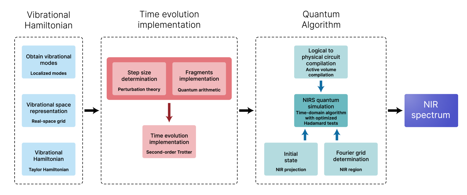
Figure 2: Workflow description for obtaining NIR spectrum on a quantum computer. Titles in bold inside sub-blocks constitute the task, with underlying text describing the associated solution. Each of the three main blocks is described in a respective subsection of Section˜III.

We now provide a full description of the quantum algorithm we propose for obtaining the NIR absorption spectrum in Eq.˜1, with a summarized description presented in Fig.˜2. When performed on an appropriate initial state, the quantum algorithm recovers not only eigenvalues of a given Hamiltonian, but directly samples the absorption spectrum while also incorporating broadening effects [qpe_xas, qpe_gqpe]. A deeper discussion of how our algorithm is connected to spectroscopy and quantum phase estimation (QPE) is presented in Ref. [qpe_gqpe], showing how to simulate linear and non-linear spectroscopic experiments on a quantum computer [qpe_gqpe]. This algorithm can be performed directly in frequency space or with a time-domain approach that performs the Fourier transform on a classical computer [qpe_lin_tong, qpe_cs, qpe_qmegs]. In this work we chose to use a time-domain implementation. An extensive optimization of all the elements that go into the algorithm was performed, allowing us to achieve a cost reduction by multiple orders of magnitude with respect to previous quantum approaches simulating vibrational systems [ibm_vibrational].

This section is organized as follows. We first explain how to construct vibrational Hamiltonians in Section˜III.1. We then describe the quantum algorithm for obtaining NIR spectra in detail in Section˜III.2. Finally, we explain all the details for implementing the time-evolution operator in Section˜III.3, noting that implementation of this operator accounts for most of the cost of the quantum algorithm.

III.1 Vibrational Hamiltonian

In this work, we choose to employ the vibrational Hamiltonian representation based on the Taylor expansion of the PES; we will refer to this as the Taylor form for brevity. The full details of how this Hamiltonian is derived from first-principles are presented in LABEL:app:taylor. This choice allows us to work with a real-space representation, which is one of the reasons for improved cost estimates for our algorithm. At the end of this section, we mention the alternative representations and briefly comment on our choice.

The starting point is the set of normal coordinates $\{q_{1},\cdots,q_{M}\}$, expressed in natural units, where each $q_{j}$ is a scalar associated with a collective displacement of the atoms. Such coordinates are normally obtained by diagonalizing the Hessian of the PES near the equilibrium geometry. Then the harmonic component of the Hamiltonian is written as

$$\hat{H}_{\rm harm}=\frac{1}{2}\sum_{j=1}^{M}\hbar\omega_{j}\left(\hat{p}_{j}^{2}+\hat{q}_{j}^{2}\right),$$ (2)

where $\hat{p}_{j}$ is the momentum operator associated with $\hat{q}_{j}$, $\omega_{j}$ is the harmonic frequency of mode $j$, and $M=3N_{\rm atoms}-6$ is the number of vibrational modes, with $M=3N_{\rm atoms}-5$ for linear molecules. The position and momentum operators follow the canonical commutation relations $[\hat{q}_{j},\hat{q}_{k}]=[\hat{p}_{j},\hat{p}_{k}]=0$ and $[\hat{q}_{j},\hat{p}_{k}]=i\hbar\delta_{jk}$. The full vibrational Hamiltonian $\hat{H}$ is then written as

$$\hat{H}=\hat{H}_{\rm harm}+\hat{H}_{\rm anh},$$ (3)

where the anharmonic component can be expressed by a Taylor expansion of the PES with respect to the normal coordinates

$$\hat{H}_{\rm anh}=\sum_{i\geq j\geq k}\Phi_{ijk}^{(3)}\hat{q}_{i}\hat{q}_{j}\hat{q}_{k}+\sum_{i\geq j\geq k\geq l}\Phi_{ijkl}^{(4)}\hat{q}_{i}\hat{q}_{j}\hat{q}_{k}\hat{q}_{l}+\cdots.$$ (4)

The Taylor coefficients can be obtained from doing a fitting of the PES; see LABEL:app:taylor for details. In the rest of this manuscript, we will refer to two attributes of a particular vibrational Hamiltonian: its maximum Taylor expansion order, which corresponds to the largest sum-total monomial power appearing in the expansion; and its $n$-mode character, where $n$ is the maximum number of distinct modes appearing together in a monomial. As an example, a Hamiltonian $\hat{H}=\hat{q}_{1}\hat{q}_{2}\hat{q}_{3}\hat{q}_{4}$ would have Taylor order four and be $4$-mode, while $\hat{H}=\hat{q}_{1}^{2}\hat{q}_{2}\hat{q}_{3}$ would also have Taylor order four while only being $3$-mode. In practice one often restricts the allowed inter-mode interactions to $3$- or even $2$-mode, while maintaining Taylor order of four: this corresponds to setting coefficients such as $\Phi_{ijkl}$ or $\Phi_{ijkk}$ to zero.

The most expensive subroutine in our algorithm is the time-evolution operator $e^{-i\hat{H}t}$. The cost of this operation is directly related to the number of terms in the Taylor expansion in Eq.˜4. Any techniques that allows us to reduce this number of terms while not hindering accuracy are particularly useful for reducing the overall cost of the quantum algorithm. In this work, we use the mode localization approach [mode_loc_1, mode_loc_2, mode_loc_3, mode_loc_4], which effectively makes the Hamiltonian more sparse and lowers the overall implementation cost. As discussed in LABEL:app:mode_loc, the usage of mode localization techniques has been shown to greatly reduce the required number of inter-mode interactions [mode_loc_1], with the example of the ethane C${}_{2}$H${}_{4}$ Hamiltonian yielding the same accuracy using a $2$-mode representation with localized modes when compared to using a $4$-mode expansion with (canonical) normal modes. By analogy to the use of localized orbitals in electronic structure calculations, mode localization redefines the vibrational modes $\hat{q}_{i}$’s so as to make the vibrations assume a more local character in the molecule. This is in contrast to the normal modes of vibration that are typically described by collective displacements of all atoms in a molecule. Mode localization yields a Hamiltonian of the form

$$\hat{H} =\sum_{i\geq j}\left(K_{ij}\hat{p}_{i}\hat{p}_{j}+\Phi_{ij}^{(2)}\hat{q}_{i}\hat{q}_{j}\right)+\sum_{i\geq j\geq k}\Phi_{ijk}^{(3)}\hat{q}_{i}\hat{q}_{j}\hat{q}_{k}$$

$$\ \ +\sum_{i\geq j\geq k\geq l}\Phi_{ijkl}^{(4)}\hat{q}_{i}\hat{q}_{j}\hat{q}_{k}\hat{q}_{l}+\cdots,$$ (5)

the main difference being the introduction of non-diagonal momentum terms. The coordinates $\hat{q}_{i}$ and coefficients $\Phi$ have been transformed, but for brevity we will use the same symbols and from now on refer exclusively to localized modes, unless explicitly stated otherwise. A more thorough discussion of how the modes are localized and the benefits of using this technique can be seen in LABEL:app:mode_loc.

We now comment on our choice of the Taylor form. Two alternative representations of the Hamiltonian are known. The most common representation is to pass from position and momentum operators $\hat{q},\hat{p}$ to the bosonic ladder operators $b,b^{\dagger}$, re-expressing the higher-order potential energy surface terms like $\hat{q}_{i}\hat{q}_{j}\hat{q}_{k}$ as powers of these creation and annihilation operators [baiardi2017vibrational]. We refer to this as the bosonic representation. A different, relatively recent approach is to use the so-called Christiansen representation (sometimes also somewhat vaguely called the occupation-number representation) first introduced in Ref. [christiansen], where the bosonic ladder of excitations for each mode is truncated and a new register is associated to each modal.

However, using the real-space representation has two concrete benefits over these second-quantized approaches. First, the real-space form discretizes each vibrational mode with exponential accuracy with respect to the used number of qubits, which alongside the compact Taylor representation of the Hamiltonian yields significantly fewer terms when compared to using a second-quantized approach. More importantly, the real-space form allows the use of highly-optimized quantum arithmetic primitives (addition and multiplication) together with the phase gradient trick to implement time-evolution [vibronic, gidney2018halving, su2021fault, quantum_arithmetic], resulting in a cheaper quantum algorithm overall. More details on the comparison between the three representations are in LABEL:app:cf_reps, and we describe how to use quantum arithmetic to implement time-evolution by the Hamiltonian in the Taylor form in Section˜III.3.

Once we have obtained the Taylor expansion constants in Eq.˜5, we need to define a qubit-based representation of the vibrational space. In this work we adopt the real-space representation as introduced in Refs. [macridin_1, macridin_2] and also used for vibrational degrees of freedom in Ref. [vibronic]. The basic idea is to have a qubit register consisting of $N$ qubits for each vibrational mode. For a given mode $q$, each of the computational basis states then encodes a point in a uniform grid that is associated to the discretization of $q$ using $2^{N}$ grid points as shown in Fig.˜3. From this we have $2^{N}$ different computational basis states for each vibrational mode: the $n$-th point in the grid for a vibrational mode $q$ has an associated computational basis state such that

$$\hat{q}\lvert n\rangle=\Delta(n-2^{N-1})\lvert n\rangle,$$ (6)

where we have defined the constant $\Delta\equiv\sqrt{2\pi/2^{N}}$ with an associated total grid width of $\sqrt{\pi 2^{N+1}}$. As thoroughly discussed in Refs. [macridin_1, macridin_2], the number of qubits $N$ required for achieving a faithful representation of vibrational excitations consisting of up to $N$ quanta in this grid scales logarithmically with respect to $N$. This exponential accuracy with respect to $N$ can be understood via the Nyquist-Shannon sampling theorem, and effectively allows for accurate encoding of the vibrational space with a small number of qubits. Applying the quantum Fourier transform (QFT) on a given mode’s qubit register is then simply a change of basis between the position and momentum representations: the transformation has the form

$$\hat{p}=\mathtt{QFT}^{\dagger}\cdot\hat{X}_{s}\cdot\hat{q}\cdot\hat{X}_{s}\cdot\mathtt{QFT},$$ (7)

where $\hat{X}_{s}$ corresponds to an $X$ gate on the most significant qubit of the register encoding the vibrational mode $q$. This $X$ gate effectively performs a “shift” in the same way as usually done for the discrete Fourier transform in classical computing, which effectively centers the Fourier transform in some range $[-a,a)$ instead of $[0,2a)$. As such we will refer to the combination $\hat{X}_{s}\cdot\mathtt{QFT}$ simply as the shifted QFT.

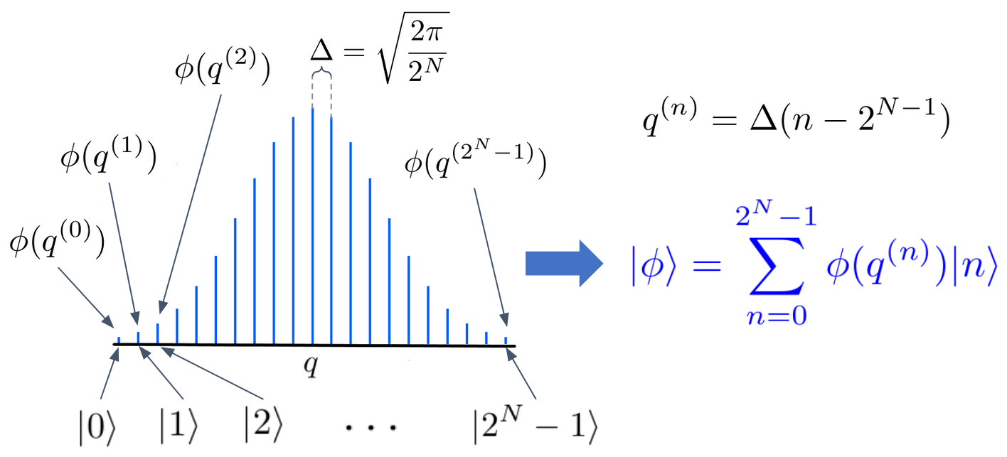
Figure 3: Real-space representation [macridin_1, macridin_2] of single vibrational mode $q$. Each of the $2^{N}$ integers associated with the $N$-qubit computational basis states are associated with a different point in the grid discretizing $q$. The wavefunction $\lvert\phi\rangle$ will then be represented by a coherent superposition over computational basis states with associated coefficients $\phi(q^{(n)})$, namely $\lvert\phi\rangle=\sum_{n}\phi(q^{(n)})\lvert q^{(n)}\rangle$.

III.2 Fourier-based algorithm for NIRS

In this section we discuss the quantum algorithm for obtaining the NIR spectrum, alongside its relationship with Fourier series, and the associated optimizations that were done in this work.

III.2.1 Fourier representation and initial state filtering

Having obtained the vibrational Hamiltonian, we can use it to obtain its absorption spectrum as shown in Eq.˜1, namely

$$\sigma_{A}(\omega)\propto\omega\sum_{\rho=x,y,z}\sum_{f}|\langle E_{f}\rvert\hat{\mu}_{\rho}\lvert E_{0}\rangle|^{2}\mathcal{L}_{\eta}(\omega-E_{f}+E_{0}).$$

As discussed in Refs. [qpe_gqpe, qpe_xas], when using an appropriate input state QPE directly samples frequencies from the associated absorption spectrum. When applied to the normalized initial state

$$\lvert\psi_{\rho}\rangle=\frac{\hat{\mu}_{\rho}\lvert E_{0}\rangle}{|\mu_{\rho}|},$$ (8)

where we use the short-hand $|\mu_{\rho}|=||\hat{\mu}_{\rho}\lvert E_{0}\rangle||$, the canonical QPE procedure returns the frequency-dependent distribution

$$P_{\rho}(\omega)=\frac{1}{|\mu_{\rho}|^{2}}\sum_{f}|\langle E_{f}\rvert\hat{\mu}_{\rho}\lvert E_{0}\rangle|^{2}\mathcal{L}(\omega-E_{f}).$$ (9)

The line shape function $\mathcal{L}(\omega)$ is linked to the initial preparation of the time/frequency register, as explained in Ref. [qpe_gqpe].

We will now show how this quantity can be expressed as a Fourier series. Before the addition of the line shape, we can write the similar Fourier integral

$$Z_{\rho}(\omega) \equiv\int_{-\infty}^{\infty}dte^{i\omega t}\langle\psi_{\rho}\rvert e^{-i\hat{H}t}\lvert\psi_{\rho}\rangle$$ (10)

$$=2\pi\sum_{f}|\langle E_{f}\rvert\hat{\mu}_{\rho}\lvert E_{0}\rangle|^{2}\delta(\omega-E_{f}).$$ (11)

From this we can obtain the target distribution as

$$P_{\rho}(\omega)=\frac{1}{2\pi|\mu_{\rho}|^{2}}Z_{\rho}(\omega)*\mathcal{L}(\omega),$$ (12)

where $*$ defines the convolution operation. Using the convolution theorem, and considering that we are targeting a Lorentzian line shape such that $\mathcal{L}(\omega)=\eta/(\omega^{2}+\eta^{2})$ with associated Fourier conjugate $e^{-\eta|t|}/2$, we arrive to

$$P_{\rho}(\omega)=\frac{1}{2\pi|\mu_{\rho}|^{2}}\int_{-\infty}^{\infty}dte^{i\omega t}\frac{e^{-\eta|t|}}{2}\langle\psi_{\rho}\rvert e^{-i\hat{H}t}\lvert\psi_{\rho}\rangle.$$ (13)

The next step is to approximate the integral on the right-hand side to some accuracy $\epsilon$ by truncating the infinite time as $\int_{-\infty}^{\infty}\rightarrow\int_{-T_{\rm max}}^{T_{\rm max}}$, which as shown in LABEL:app:max_time can be done by choosing

$$T_{\rm max}=\frac{1}{\eta}\log\frac{1}{\epsilon}.$$ (14)

This finite integral can now be expressed using a Fourier series. Noting that $P_{\rho}(\omega)$ is localized inside of some spectral range $[\omega_{\rm min},\omega_{\rm max}]$, we can use a finite Fourier series to expand $P_{\rho}(\omega)$, effectively making it periodic outside of this range. Defining the spectral width as $\Omega=\omega_{\rm max}-\omega_{\rm min}$, this effectively defines a Fourier grid for a discrete Fourier transform. We thus obtain the Fourier series approximation of the target distribution

$$P_{\rho}(\omega)\approx\frac{1}{\Omega|\mu_{\rho}|^{2}}\left[\frac{1}{2}+\sum_{k=1}^{k_{\rm max}}\operatorname{Re}\left(p_{\rho}[k]e^{2\pi ik\omega/\Omega}\right)\right]$$ (15)

where the number of Fourier coefficients is

$$k_{\rm max}=\lceil\Omega\cdot T_{\rm max}\rceil$$ (16)

and we defined the Fourier components

$$p_{\rho}[k]=e^{-2\pi\eta k/\Omega}\langle\psi_{\rho}\rvert e^{-2\pi i\hat{H}k/\Omega}\lvert\psi_{\rho}\rangle.$$ (17)

The unitary that is entering the expectation value is $e^{-2\pi i\hat{H}k/\Omega}$, which can also be thought as rescaling the Hamiltonian $\hat{H}\rightarrow\hat{H}/\Omega$ to effectively estimate the phase of $\hat{H}/\Omega$. Typically a rescaling factor $\Omega\sim\mathcal{O}(||\hat{H}||^{-1})$ is used in order to keep the spectrum in the $[-1,1]$ range and avoid aliasing in the Fourier transform that comes from making the $P_{\rho}(\omega)$ function periodic when approximating it as a Fourier series.

However, in this work we are focusing in the NIR spectrum, which consists of the range of frequencies between $4,000$ and $12,500$ cm${}^{-1}$. As seen in Fig.˜4, the mid-IR region compromises the largest absorption peaks, while the NIR region has peaks coming from overtones and combination bands that quickly decay as the excitation energy increases, while no significant vibrational excitations happen beyond this region. Since our interest is in the NIR region, it becomes unnecessary to simulate the mid-IR portion. Still, if we choose the Fourier frequency window to be only in the NIR range, the non-zero spectrum coming from mid-IR would appear as an aliasing effect due to the periodic nature of the Fourier series. In order to avoid simulating any peaks from this region, we propose a filtering procedure over the initial state $\lvert\psi_{\rho}\rangle$, which can be written in the eigenstate basis as

$$\lvert\psi_{\rho}\rangle=\sum_{k}a_{k}^{(\rho)}\lvert E_{k}\rangle.$$ (18)

The idea is to set to zero all $a_{k}^{(\rho)}$ with associated energies $E_{k}$’s outside of the NIR range. This can be written as the condition $\omega_{k0}<4,000\textrm{ cm}^{-1}$, where we have defined the excitation energy $\omega_{k0}\equiv E_{k}-E_{0}$. However, in practice we obviously do not have access to the exact eigenstates and energies. To circumvent this we start by considering some approximate eigenstates $\lvert\tilde{E}_{k}\rangle$, which in this work we obtain from the mean-field method VSCF [vscf_1, vscf_2, vscf_3, vscf_4]. We then expand the wavefunction in this basis as $\lvert\psi_{\rho}\rangle=\sum_{k}\tilde{a}_{k}^{(\rho)}\lvert\tilde{E}_{k}\rangle$. Due to the approximate nature of these eigenstates and in order to avoid removing components that could appear in the NIR spectrum, we used a padding of $250{\rm\ cm^{-1}}$, noting that VSCF energies typically approximate the exact energies in the mid-IR region within $\sim 100$ cm${}^{-1}$ [beyond_vscf]. We thus chose an energy cutoff value of $W=3,750$ cm${}^{-1}$. By considering the projector

$$\hat{\Pi}_{W}=\sum_{k|\tilde{\omega}_{k0}\geq W}\lvert\tilde{E}_{k}\rangle\langle\tilde{E}_{k}\rvert,$$ (19)

we can pass the (renormalized) initial state $\hat{\Pi}_{W}\lvert\psi_{\rho}\rangle$ to our algorithm to focus on the NIR region. From this consideration, we chose to simulate the window in the spectral range between $\omega_{\rm min}=3,500\textrm{ cm}^{-1}$ and $\omega_{\rm max}=12,500$ cm${}^{-1}$ as to guarantee that no absorption line coming from the mid-IR region appears as an aliasing component in our recovered spectrum. This yields the spectral width

$$\Omega=9,000\textrm{ cm}^{-1}.$$ (20)

Besides allowing us to simulate only the NIR region with the smaller $\Omega$, which translates to smaller $k_{\rm max}$ and maximum evolution times, the removal of these states in the mid-IR entails a renormalization of the initial wavefunction by a factor of $|\hat{\Pi}_{W}\lvert\psi_{\rho}\rangle|$. The spectrum obtained with the initial wavefunction $\hat{\Pi}_{W}\lvert\psi_{\rho}\rangle/|\hat{\Pi}_{W}\lvert\psi_{\rho}\rangle|$ carries a division by $||\hat{\Pi}_{W}\lvert\psi_{\rho}\rangle||^{2}$ when compared to the one obtained with $\lvert\psi_{\rho}\rangle$ in Eq.˜15. The overall accuracy in the NIR region is thus boosted by a factor of $||\hat{\Pi}_{W}\lvert\psi_{\rho}\rangle||^{-2}$. This manifests as a large improvement in the accuracy requirements by around two to six orders of magnitude: the $\hat{\mu}_{\rho}\lvert E_{0}\rangle$ optical excitation is typically constituted by $90$ to $99.9\%$ of states coming from the mid-IR region.

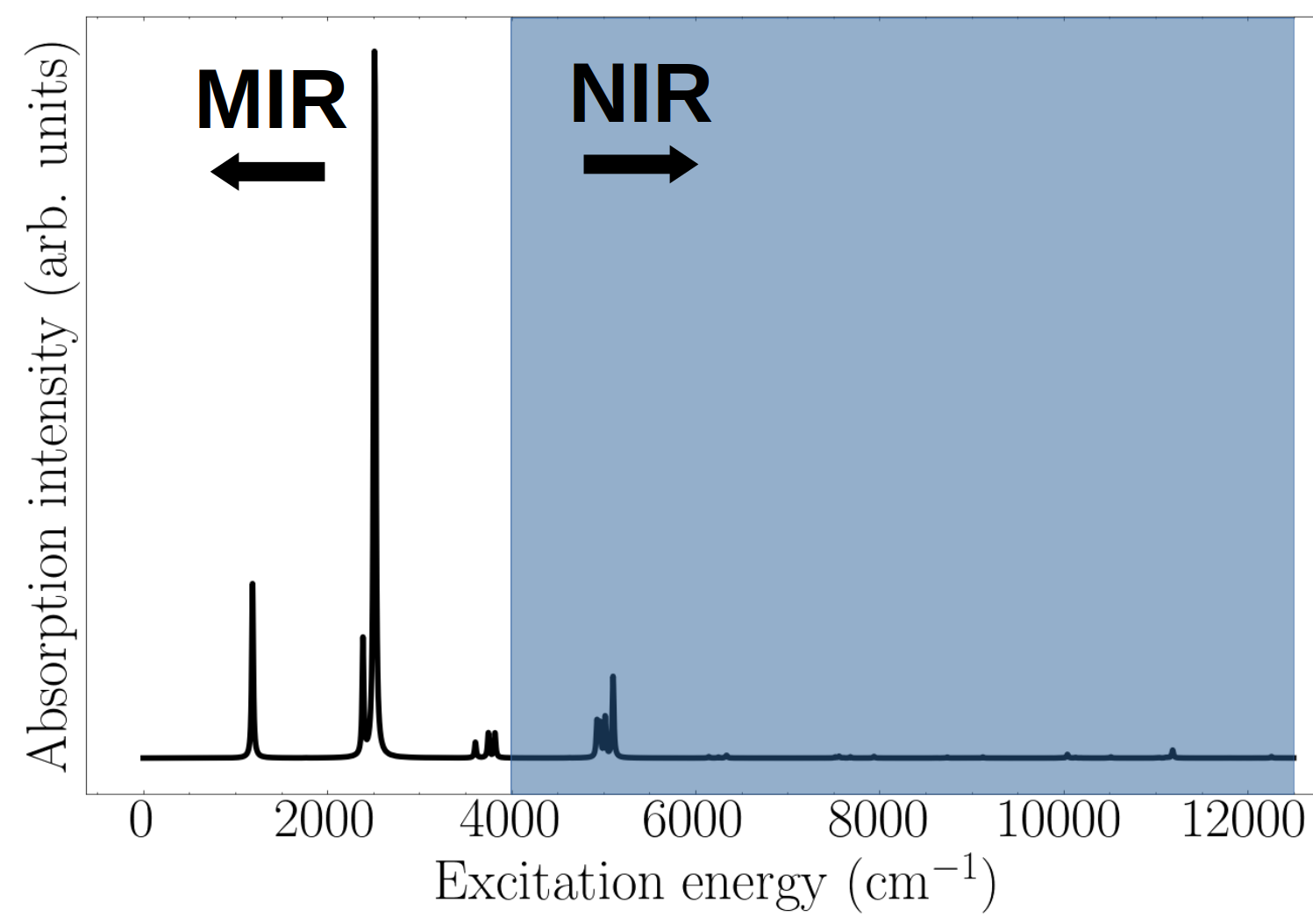
Figure 4: Simulated spectrum of hydrogen sulfide H${}_{2}$S molecule. Note how the amplitudes of the near-IR spectrum are significantly smaller than those of the mid-IR: the former come from overtones and combination bands, having a strong anharmonic character that is classically challenging to simulate.

Before continuing the discussion of the algorithm, we now explain why using a product formula implementation of the time-evolution operator is more attractive than using a qubitization-based framework [qubitization, qrom, mtd, walk_based_qpe]. Of particular interest for this comparison is the ability to focus on the NIR spectral region in our product-formula-based implementation. Being able to focus in some particular spectral region cannot be easily done when performing the so-called “walk-based QPE” approach [qrom], noting that walk-based QPE constitutes a more efficient approach for qubitization-based QPE when compared to direct implementation of the time-evolution operator through the Jacobi-Anger expansion [qubitization]. Qubitization necessitates the rescaling of the entire spectrum of $\hat{H}$ to the range $[-1,1]$ through the appearance of the 1-norm $\lambda$, where the operator $\hat{H}/\lambda$ is effectively implemented as to keep the block-encoding unitary [LCU4]. However, in practice most of the absorption in this rescaled spectrum will be trivially zero. This happens since the representation used for the Hamiltonian will have many states that are never excited but with extremely high energies. An example of such a state would correspond to having all the amplitude of a given state in the real-space representation appearing only in the borders of the grid. From this we can assert that as the system size grows and more of these states become available, $\lambda$ will quickly increase, whereas our chosen $\Omega$ has a constant value of $9,000\textrm{ cm}^{-1}$ associated with the NIR region, which is the only region where there will be some absorption after the state projection procedure. Rescaling by $\Omega$ instead of $\lambda$ then enables a vastly increased resolution in the energy x-axis. This consideration makes product-formula-based implementations of QPE-based algorithms for spectroscopy particularly attractive.

III.2.2 Time-domain quantum algorithm

Having shown how to express the target distribution as a Fourier series with associated coefficients $p_{\rho}[k]$ in Eq.˜17, these now need to be determined for each of $k=1,\cdots,k_{\max}$. The $e^{-2\pi\eta k/\Omega}$ factor makes contributions from large $k$’s vanishingly small, which in turn means that there is no need to determine the associated $p_{\rho}[k]$’s to the same high accuracy as those coming from smaller $k$’s. Overall, we will allocate a number of shots proportional to $e^{-2\pi\eta k/\Omega}$ to determine the associated $p_{\rho}[k]$, which as seen below allows us to seamlessly incorporate the Lorentzian line shape while also having a fixed accuracy for each $p_{\rho}[k]$ component.

The key component of the time-domain formulation of the algorithm is the expectation value of the self-correlation function$\langle\psi_{\rho}\rvert e^{-i\hat{H}t}\lvert\psi_{\rho}\rangle$. Shown in Fig.˜5 is the Hadamard test quantum circuit for recovering this quantity through the implementation of the time-evolution for a given time $t$: the ancilla qubit encodes the expectation value of interest as

$$p_{0}(t)-p_{1}(t)=\operatorname{Re}\left[{\langle\psi_{\rho}\rvert e^{-i\hat{H}t}\lvert\psi_{\rho}\rangle}\right].$$ (21)

The imaginary component can be obtained instead if the gate in the Hadamard test after the controlled time-evolution is $S^{\dagger}$ instead of $I$. Here $p_{0}(t)$ and $p_{1}(t)$ are the probabilities of observing the ancilla in state $0$ and $1$ respectively for the controlled time-evolution $e^{-i\hat{H}t}$.

[row sep=0.4cm] $\lvert 0\rangle$ H 1 I/S^† H
$\lvert\psi_{\rho}\rangle$ e^-i^H t

Figure 5: Hadamard test circuit for a given evolution time $t$. By obtaining expectation values over a range of times and performing the Fourier transform on classical hardware Eq.˜9 is recovered.

As shown in Refs. [qpe_qmegs, qpe_gqpe, qpe_lin_tong], if we consider a total number of shots $\mathcal{S}$, we can then run the Hadamard test circuit in Fig.˜5 for a time $t=2\pi k/\Omega$ a total of

$$\mathcal{N}_{k}=\mathcal{S}\mathcal{N}e^{-2\pi\eta k/\Omega}$$ (22)

times for both the real and imaginary components, where $\mathcal{N}=\left[2\sum_{k=1}^{k_{\max}}e^{-2\pi\eta k/\Omega}\right]^{-1}$ is a normalization constant. The $m$-th pair of real/imaginary measurements of the ancilla qubit with associated $k=k_{m}$ then yields the numbers $x_{\rho}^{(m)}$ and $y_{\rho}^{(m)}$. Here we have assigned a value of $1(-1)$ to the random variables $x_{\rho}^{(m)}$ and $y_{\rho}^{(m)}$ when the associated measurement of the Hadamard test ancilla qubit corresponds to $0(1)$, which implies that $\langle\psi_{\rho}\rvert e^{-2\pi i\hat{H}k/\Omega}\lvert\psi_{\rho}\rangle=\mathbb{E}\left[{x_{\rho}^{(m)}+iy_{\rho}^{(m)}}\right]$ . The non-uniform sampling over $k$’s then incorporates the line shape contribution to the spectrum, recovering the target spectrum as

$$P_{\rho}(\omega) \approx\frac{1}{\Omega|\mu_{\rho}|^{2}}\left[\frac{1}{2}+\frac{1}{\mathcal{N}_{0}}\sum_{m=1}^{\mathcal{S}/2}\operatorname{Re}\left[\left(x_{\rho}^{(m)}+iy_{\rho}^{(m)}\right)e^{2\pi ik\omega/\Omega}\right]\right],$$ (23)

where $\mathcal{N}_{0}$ corresponds to considering Eq.˜22 for $k=0$. To better understand the effect of the variable number of shots in the determination of the spectrum, we now provide a bound of the variance associated with the Fourier components of the spectrum [Eq.˜17], namely $p_{\rho}[k]=e^{-2\pi\eta k/\Omega}\cdot\mathbb{E}\left[x_{\rho}^{(m)}+iy_{\rho}^{(m)}\right]$. The variance after considering $\mathcal{N}_{k}$ samples of these random variables is

$${\rm Var}(p_{\rho}[k]) =\frac{1}{\mathcal{N}_{k}^{2}}[e^{-2\pi\eta k/\Omega}]^{2}\cdot{\rm Var}(x_{\rho}^{(m)}+iy_{\rho}^{(m)})$$ (24)

$$\leq\frac{1}{(\mathcal{SN})^{2}}\cdot\mathbb{E}\left[|x_{\rho}^{(m)}|^{2}+|y_{\rho}^{(m)}|^{2}\right]$$ (25)

$$=\frac{2}{(\mathcal{SN})^{2}}.$$ (26)

From this analysis we can see how the $k$-dependent shot allocation in Eq.˜22 entails a fixed maximum variance over all the different Fourier components of the spectrum.

We note that some approaches have been proposed for post-processing the obtained spectrum in Eq.˜23 by using, e.g., a matching pursuit algorithm [qpe_qmegs], which can be effectively used to remove the noise coming from finite sampling. Determination of $\mathcal{S}$ is purely a signal processing problem, corresponding to the accuracy that is required for the coefficients of a Fourier series to recover the associated signal to some accuracy, with the main quantities that determine the signal being the line shape width $\eta$ and the spectral range $\Omega$. In practice we use the quantity $\mathcal{S}_{\rm tot}=3\mathcal{S}$ to account for all three Cartesian components of the dipole appearing in the absorption spectrum. Practical choices of $\mathcal{S}_{\rm tot}$ are obtained heuristically in LABEL:sec:benchmark.

III.2.3 Hadamard test optimizations

Having shown how a measurement of the expectation values in Eq.˜21 through the Hadamard test can be used to recover the NIR spectrum, we now discuss two additional optimizations that effectively diminish the required evolution times when implementing $e^{-i\hat{H}t}$ and the required number of circuit repetitions [new_xas].

Double measurement method.

The basic idea is to re-use the output state after applying the Hadamard test to gain additional information of the associated expectation value. After performing the Hadamard circuit in Fig.˜5, by undoing the initial state preparation in the system register and measuring the system qubits we can increase the amount of information that is recovered from each Hadamard test. The circuit for performing this can be seen in Fig.˜6. For simplicity in this discussion we assume that the Hadamard test was ran obtaining the real part, noting that an analogue analysis can be done for the imaginary component. The full details of this procedure are shown in Ref. [new_xas].

We start by noting that the output state of the Hadamard test corresponds to

$$\lvert\Psi_{\rho}^{\pm}\rangle=\frac{(\hat{I}\pm\hat{U})\lvert\psi_{\rho}\rangle}{\sqrt{\langle\psi_{\rho}\rvert(1\pm\hat{U})^{\dagger}(1\pm\hat{U})\lvert\psi_{\rho}\rangle}},$$ (27)

where the $\pm$ sign is determined by the outcome from measuring the Hadamard test ancilla qubit. After applying the hermitian conjugate of the initial state preparation $\hat{U}_{\rho}$ on the system, which acts as $\hat{U}_{\rho}\lvert\vec{0}\rangle=\lvert\psi_{\rho}\rangle$, the probability of measuring all $0$’s in the system register then corresponds to

$$p^{(\pm)}_{\vec{0}}=\frac{|1\pm\langle\psi_{\rho}\rvert\hat{U}\lvert\psi_{\rho}\rangle|^{2}}{2(1\pm{\rm Re}\langle\psi_{\rho}\rvert\hat{U}\lvert\psi_{\rho}\rangle)}.$$ (28)

The full analysis of how this technique lowers the overall cost is presented in Ref. [new_xas]: the result is that the overall number of shots is reduced by a factor $\zeta\in[1,3.00]$, the factor being determined by the expectation value being measured – with an average reduction of $\zeta=1.49$.

[row sep=0.4cm] $\lvert 0\rangle$ H 1 I/S^† H n
$\lvert\vec{0}\rangle$ U_ρ U U_ρ^†

Figure 6: Double measurement Hadamard circuit which un-prepares the initial state and then measures the output of the Hadamard circuit, returning additional information about the expectation value $\langle\psi_{\rho}\rvert\hat{U}\lvert\psi_{\rho}\rangle$.

Double phase method.

The main idea of this method [new_xas, qrom, double_phase] is to change the controlled unitary that the Hadamard test implements as

$$\begin{bmatrix}\hat{1}&0\\ 0&e^{-i\hat{H}t}\end{bmatrix}\rightarrow\begin{bmatrix}e^{i\hat{H}t}&0\\ 0&e^{-i\hat{H}t}\end{bmatrix},$$ (29)

as shown in Fig.˜7. The benefit of doing this is that the ancilla qubit now encodes the expectation value of $e^{-2i\hat{H}t}$ instead of the $e^{-i\hat{H}t}$ term seen in Eq.˜21, which implies recovering the expectation value for an evolution time that is twice as long. Moreover, implementing the unitary corresponding to Eq.˜29 can be done for an even lower cost than the controlled time-evolution in the original Hadamard test. To understand this improvement, we start by considering the original Hadamard test, for which controlling the time-evolution simply necessitates controlling the addition operation to the circuit shown in LABEL:fig:poly_evolution. As explained in Section˜III.3, the coefficients coming from the Taylor expansion, e.g. $\Phi_{ij}^{(2)}$, are encoded in a quantum register, with the associated $e^{i\Phi_{ij}^{(2)}\hat{q}_{i}\hat{q}_{j}}$ operator then implemented using the phase kickback technique [phase_gradient]. Thus, instead of having to control the addition operation, the unitary in Eq.˜29 for the modified Hadamard test can be implemented by simply flipping the qubit that encodes the sign of the $\Phi_{ij}^{(2)}$ coefficient, which is done using a $\mathtt{CNOT}$ gate. When we also consider the uncomputation cost (see LABEL:fig:poly_evolution) the modified unitary in Eq.˜29 can be implemented with the same cost of the uncontrolled application of $e^{-i\hat{H}t}$, plus $2N_{\rm Taylor}$ $\mathtt{CNOT}$ gates, where $N_{\rm Taylor}$ is the total number of non-zero coefficients appearing in the Hamiltonian in Eq.˜4. This basically allows to implement the required time-evolutions for half the cost.

[row sep=0.4cm] $\lvert 0\rangle$ H 1 1 I/S^† H
$\lvert\psi_{\rho}\rangle$ e^-i^H t e^+i^H t

Figure 7: Double phase circuit which effectively doubles the time-evolution length on the Hadamard test in Fig.˜5.

III.2.4 Active volume compilation

The active volume compilation technique was introduced in Ref. [active_volume]. At an abstract algorithmic level, it can be thought of as reducing the time and resources needed to run quantum algorithms on a specific error-corrected hardware architecture. The basic idea is based on the observation that during typical computations, most of the qubits at any given time are idle. However, the computation cost is usually determined by the circuit volume, this being the number of qubits multiplied by the number of non-Clifford gates. By using additional qubits to compute chunks of logical operations that can be parallelized, these can then be applied via teleportation. The active volume is then determined by the number of logical operations making up these chunks, where each particular logical operation has an associated active volume that is measured in so-called blocks.

The overall cost of the computation is then dictated by the number of blocks instead of the circuit volume, which typically leads to one or more orders of magnitude reduction of the overall computation time. Note that the active volume compilation also already incorporates error correction for fault-tolerance through the surface code. The usage of this technique for runtime optimization and estimation reflects the kind of techniques that we expect could be used to compile our algorithm on a physical level, having that the specific technique and associated estimates would need to be tailored to the specific hardware under consideration.

The active volume compilation divides the qubits into two groups: working qubits and memory qubits. Memory qubits are used to accelerate the calculation by parallelizing blocks and storing intermediate results or ancillary states which are used in subsequent steps of the computation. The speed-up from the active volume can be estimated through the following steps:

1. Identify the required number of logical qubits for implementing a circuit of interest $Q_{L}$. For a given budget of logical qubits $Q_{B}$, set the number of working qubits as $Q_{W}=\lfloor Q_{B}/2\rfloor$. Note that the active volume compilation technique requires that $Q_{W}\geq Q_{L}$, thus at least duplicating the required number of logical qubits. The memory qubits are then allocated as $Q_{M}=Q_{W}$.

2. Calculate the active volume in blocks $B$ for the quantum algorithm of interest. This is done by first decomposing the algorithm into elementary subroutines, which are in turn decomposed into a block-based implementation. This procedure for decomposing into blocks is covered in details in Ref. [active_volume], with Table 1 summarizing the cost of most commonly used subroutines.

3. Divide the number of blocks by the number of memory qubits: this will approximate the required number of cycles to implement all operations as $N_{\rm cycles}=B/Q_{M}$. Note that the block-based implementation of the circuit already includes error correction through the use of a surface code, making the associated improvement unable to be converted back to elementary logical gates.

4. Divide the number of cycles by the clock-rate $\nu_{\rm clock}$ to obtain the total runtime of the circuit $T_{\rm runtime}=N_{\rm cycles}/\nu_{\rm clock}$.

It should be emphasized that the above constitutes a high-level description of the procedure, with additional considerations being necessary for a complete description of the active volume compilation technique. However, for the purposes of this work our description is sufficient for obtaining reasonable runtime estimates while also exploiting the associated speed-up of using the active volume compilation.

III.3 Time-evolution implementation

Having described both the quantum algorithm and the qubit mapping of the vibrational degrees of freedom, the only missing piece of the workflow is the implementation of the time-evolution operator $e^{-i\hat{H}t}$ and the circuit for initial state preparation corresponding to $\lvert\psi_{\rho}\rangle$ in Eq.˜8. As discussed in LABEL:app:init_state, this initial state can be efficiently prepared at a cost that is negligible compared with that of implementing the time-evolution. This can be understood since a small number of mean-field VSCF states can be used to represent the initial state: the initial state is extremely sparse in this basis. Given that, we now focus on the implementation of the time-evolution operator. We start by separating the Hamiltonian into its kinetic and potential components $\hat{H}=\hat{T}+\hat{V}$, where

$$\hat{T} =\sum_{i\geq j}K_{ij}\hat{p}_{i}\hat{p}_{j}=\mathtt{Q_{M}}^{\dagger}\left(\sum_{i\geq j}K_{ij}\hat{q}_{i}\hat{q}_{j}\right)\mathtt{Q_{M}}$$ (30)

$$\hat{V} =\sum_{i\geq j}\Phi_{ij}^{(2)}\hat{q}_{i}\hat{q}_{j}+\sum_{i\geq j\geq k}\Phi_{ijk}^{(3)}\hat{q}_{i}\hat{q}_{j}\hat{q}_{k}$$

$$\ \ +\sum_{i\geq j\geq k}\Phi_{ijkl}^{(4)}\hat{q}_{i}\hat{q}_{j}\hat{q}_{k}\hat{q}_{l}+\cdots,$$ (31)

where we have defined the multidimensional shifted QFT as the product of shifted QFT s over all modes:

$$\mathtt{Q_{M}}=\prod_{j=1}^{M}\hat{X}_{s,j}\cdot\mathtt{QFT}_{j}.$$ (32)

The operator $\hat{V}$ is already diagonal in the real-space representation, while conjugation with $\mathtt{Q_{M}}$ makes the kinetic term diagonal. We can then use a second-order Trotter formula to approximate the time-evolution as

$$e^{-i\hat{H}t}\approx e^{-i\hat{V}\frac{t}{2}}e^{-i\hat{T}t}e^{-i\hat{V}\frac{t}{2}}\equiv\hat{\mathcal{U}}_{2}(t).$$ (33)

In this work we chose a second-order Trotter formula since it was associated with the lowest implementation costs for achieving the required accuracy in our test systems when compared to other Trotter orders. The required evolution time for the unitary corresponding to a single time step, namely $e^{-2\pi i\hat{H}/\Omega}$, is not too long. This makes the required Trotter evolution time relatively short, which tends to benefit lower order Trotter formulas. We will refer to $\hat{\mathcal{U}}_{2}(t)$ as the Trotter oracle.

III.3.1 Trotter step size determination

Many works have addressed the problem of bounding the error to estimate the associated Trotterization cost that achieves a target accuracy [trotter_error, trotter_pt, trotter_pt_2]. However, the resulting upper bounds to the Trotter error are known to be overly pessimistic [trotter_error, trotter_error_1, trotter_error_2, trotter_error_3], with tighter estimates such as direct simulations requiring a prohibitive amount of classical resources to be obtained. One of the main contributions of this work is an alternative, cheaper-to-implement approach to more tightly control the Trotter error: instead of aiming to upper-bound the error, we estimate it using an approach based on perturbation theory. This tighter estimate is in turn used to obtain a less pessimistic step size for the Trotterized time-evolution, strongly reducing the associated cost of implementing the time-evolution operator. Inspired by the perturbation-based approach of Refs. [trotter_pt, trotter_pt_2] to estimate the Trotter error for ground-state properties, in this work we extend it to include excited states and consider a second-order Trotter formula. Still, all the discussion that follows can be straightforwardly extended to arbitrary product formulas.

We start by remembering that our algorithm for spectroscopy can be considered to an extent as performing phase estimation on the operator $2\pi\hat{H}/\Omega$. For convenience we define $\Delta t=2\pi/\Omega$, working with the operator $\hat{H}\Delta t$. The Trotterized time-evolution operator effectively implements a time evolution under an effective Hamiltonian, namely $e^{-i\hat{H}_{\rm eff}\Delta t}$. We thus need to make the eigenvalues of $\hat{H}_{\rm eff}$ that contribute to the absorption spectrum to be the same as those of $\hat{H}$ within some target accuracy $\epsilon_{\nu}$. To achieve this, we start by partitioning the Trotterized time-evolution into $r$ steps, from which we can write

$$e^{-i\hat{H}_{\rm eff}\Delta t}=\left[\hat{\mathcal{U}}_{2}\left(\frac{\Delta t}{r}\right)\right]^{r}.$$ (34)

Using the Baker-Campbell-Hausdorff formula we then arrive to

$$\hat{H}_{\rm eff}=\hat{H}+\left(\frac{\Delta t}{r}\right)^{2}\hat{\mathcal{E}}_{2}+\mathcal{O}\left(\frac{\Delta t^{4}}{r^{4}}\right).$$ (35)

Here we have defined the error operator

$$\hat{\mathcal{E}}_{2}=\frac{1}{24}\left(2[\hat{T},[\hat{T},\hat{V}]]+[\hat{V},[\hat{T},\hat{V}]]\right);$$ (36)

different fragmentation techniques for the Hamiltonian would yield different error operators depending also on nested commutators. In the above, we adopt the straightforward fragmentation into kinetic and potential energy fragments shown in Eq.˜33. We can now use perturbation theory to estimate the eigenvalues of $\hat{H}_{\rm eff}$ [trotter_pt, trotter_pt_2]. The explicit dependence on $\Delta t/r$ will make different degrees of perturbation theory be associated with different powers of $\Delta t/r$. First order perturbation theory is enough in this case to obtain the leading order. We thus obtain the eigenvalues of $\hat{H}_{\rm eff}$

$$E_{j}^{(\textrm{eff})}=E_{j}+\frac{\Delta t^{2}}{r^{2}}\langle E_{j}\rvert\hat{\mathcal{E}}_{2}\lvert E_{j}\rangle+\mathcal{O}\left(\frac{\Delta t^{4}}{r^{4}}\right),$$ (37)

which deviate from the true eigenvalues depending on the chosen step size $r$. For simplicity we now define the time step size $\tau_{j}=\Delta t/r$ such that the associated error is within some threshold, namely $|E_{j}^{(\textrm{eff})}-E_{j}|<\epsilon_{\nu}$. Note that the $\Delta t/r$ factor is not always smaller than one for the chosen $\Delta t$ and $r$’s in this work, meaning in principle we would need to consider higher-order contributions. However, choosing $r$ as to make the leading order error smaller than $\epsilon_{\nu}$ causes the remaining terms to be small as well, as long as $\epsilon_{\nu}$ is not too large. As shown in the simulations in LABEL:sec:benchmark, reasonable choices of $\epsilon_{\nu}$ yield high-quality spectra. From this, we obtain

$$\tau_{j}=\sqrt{\frac{\epsilon_{\nu}}{\langle E_{j}\rvert\hat{\mathcal{E}}_{2}\lvert E_{j}\rangle}}.$$ (38)

The physical interpretation of $\tau_{j}$ is as the largest time step that can be taken with the Trotterized time-evolution such that eigenvalue $E_{j}^{({\rm eff})}$ of the effective Hamiltonian is within the allowable error threshold $\epsilon_{\nu}$ from the true eigenvalue $E_{j}$. Since the initial state given in Eq.˜18 only has significant contributions from a small number of eigenstates and our final target quantity is the associated absorption spectrum, we can then choose to only account for the eigenstates making up the initial state: errors in the energies of optically inactive states will not affect the quality of the spectrum. We then choose to include each of the eigenstates with a weight associated to its overlap with the initial state $\lvert\psi_{\rho}\rangle$ in Eq.˜8, namely

$$\tau=\sum_{j}|\langle E_{j}\rvert\psi_{\rho}\rangle|^{2}\tau_{j},$$ (39)

where for simplicity we here used the same $\tau$ for all three Cartesian components $\rho=x,y,z$ by averaging the associated $\tau$’s. All of these expressions are in terms of exact eigenstates, which are obviously not accessible for systems of interest. To circumvent this, we can use approximate eigenstates as done in the initial state projection procedure. Once $\tau$ has been obtained, we can recover the associated number of Trotter steps as

$$r=\left\lceil\frac{\Delta t}{\tau}\right\rceil.$$ (40)

The inclusion of the overlap factor in Eq.˜39 makes it unnecessary to calculate the expression in Eq.˜38 for all $j$’s: it only needs to be evaluated whenever there is a significant overlap $|\langle E_{j}\rvert\psi_{\rho}\rangle|^{2}$. The expectation values corresponding to $\langle E_{j}\rvert\hat{\mathcal{E}}_{2}\lvert E_{j}\rangle$ can be efficiently approximated by using states obtained from VSCF and representing the $\hat{T}$ and $\hat{V}$ operators using bosonic ladder operators. The expectation value computed in this way might differ from one expressed in the real-space basis, because the commutator algebra of the discrete operators $\hat{q}_{j},\hat{p}_{j}$ agrees with that of the infinite-dimensional bosonic operators $b_{j},b_{j}^{\dagger}$ only on a finite low-energy subspace [macridin_1, macridin_2]. However, as long as enough points were used to discretize the vibrational modes when building the real-space representation, this low-energy subspace of agreement encompasses the optically active region of interest. This condition was already met when discretizing the real-space grid.

III.3.2 Implementing time-evolution of a fragment

[row sep=0.4cm] $\lvert q_{i}\rangle$ N [3]   Mult    $a$ $a$ [3]   Mult^†    $a$ $a$ $\lvert q_{i}\rangle$
$\lvert q_{j}\rangle$ N $b$ $b$ $b$ $b$ $\lvert q_{j}\rangle$
$\lvert\vec{0}\rangle$ 2N $0$ $ab$ [3]   Mult   $a$ $a$ [3]   Mult^†   $a$ $a$ $ab$ $0$ $\lvert\vec{0}\rangle$
$\lvert\vec{0}\rangle$ b_k →X(Φ_ij) $b$ $b$