A $\nu$ look at the Sun: Probing the conditions of the solar core using ⁸B neutrinos

Abstract

In the coming age of precision neutrino physics, neutrinos from the Sun become robust probes of the conditions of the solar core. Here, we focus on ⁸B neutrinos, for which there are already high precision measurements by the Sudbury Neutrino Observatory and Super-Kamiokande. Using only basic physical principles and straightforward statistical tools, we calculate projected constraints on the temperature and density of the ⁸B neutrino production zone compared to a reference solar model. We outline how to better understand the astrophysics of the solar interior using forthcoming neutrino data and solar models. 

I Introduction

The Sun is a foundational source in nuclear astrophysics [1, 2, 3, 4, 5]. A longstanding program uses neutrino observations [6, 7, 8, 9, 10, 11, 12, 13, 14] to directly probe the nuclear reactions that power the Sun’s sustained luminosity [15, 16, 17]. Each of its nuclear-reaction chains produces a distinctive neutrino spectrum (depending upon laboratory nuclear physics) and flux (depending also upon the astrophysics of the solar interior) [18, 19, 20, 21, 22, 23, 24]. Success in this program is crucial to understanding all other main-sequence stars, for which we expect no direct observations of neutrinos and must therefore rely upon electromagnetic observations and theoretical modeling [25, 26, 27, 28, 29, 30, 31, 32].

For several decades, this program was interrupted by the (exciting) diversion of the solar neutrino problem. In 1968, the first results from the Homestake radiochemical neutrino detection experiment showed a solar electron neutrino flux well below expectations from solar models [6]. This tension persisted throughout efforts to better understand uncertainties in solar-model and nuclear physics, plus subsequent measurements of the neutrino flux. While proposed solutions to the solar neutrino problem included non-standard solar models, ultimately the correct answer was neutrino flavor mixing, which was first proposed for neutrinos in vacuum by Pontecorvo [33] and later expanded to include matter effects by Mikheyev, Smirnov, and Wolfenstein (MSW) [34, 35]. The definitive discovery of mixing was made by the Sudbury Neutrino Observatory (SNO), additionally confirming that the total ⁸B neutrino flux agrees with predictions [11, 36]. Furthermore, the Kamiokande Liquid Scintillator Anti-Neutrino Detector (KamLAND) reactor experiment measured neutrino mixing parameters consistent with the large mixing angle oscillation (LMAO) solution for the MSW effect in the Sun [37, 38, 39], up to some modest tension in the mass-squared splitting.

We will soon have an opportunity to return to the original program of probing the astrophysics of the solar core [15, 16, 17]. Doing so may help resolve persistent discrepancies in solar helioseismology [40, 41, 42, 43] and metallicity data [44, 45, 46]. The Jiangmen Underground Neutrino Observatory (JUNO), starting operations in 2025, will improve uncertainties on some neutrino mixing parameters from 3–10% to better than 1% [47, 48]. Beyond that, new experiments, especially Hyper-Kamiokande [49, 50, 51] and the Deep Underground Neutrino Experiment (DUNE) [52, 53, 54, 55, 56, 57, 58], will greatly improve the precision of other neutrino mixing parameters. In the absence of indications of new physics, we therefore expect that the neutrino mixing parameters will be precisely known, independent of solar-neutrino data. What, then, can solar-neutrino observations teach us about solar astrophysics?

In this paper, we work towards model-independent probes of the astrophysics of the solar core based on neutrino data, improving upon earlier work [59, 60, 61, 62, 63, 64]. We focus on ⁸B neutrinos, relying only on basic physical principles and straightforward statistics. There are two basic ideas behind our work. First, the total flux of ⁸B neutrinos is very sensitive to the temperature of the solar core: $\phi\propto T_{\textrm{c}}^{\alpha}$, with $\alpha\sim 24$ [65]. Because SNO has measured the total ⁸B neutrino flux to better than 10% [36], this probes the solar core temperature to better than 1%. Second, because of how neutrinos mix, the electron neutrino survival probability at Earth depends on the solar density at production. For ⁸B neutrinos, this effect becomes important at the low-energy end of the spectrum of scattered electrons in Super-Kamiokande (Super-K). Their most recent results — using the full data period of Super-K-IV [66] — thus allow for the best chance yet to probe the conditions of the solar core.

In Sec. II, we calculate how the spectrum of scattered electrons in Super-K depends on the details of ⁸B production, propagation, and detection. In Sec. III, we present our major result: the first combination of constraints on solar structure in the plane of density and temperature, ($\rho,T$). While simple, this is new and provides important insights. We also outline broader studies of the solar core conditions. Finally, in Sec. IV, we conclude and look towards the future of the solar astrophysics program.

II Calculation of the ⁸B signal

In this section, we present our calculations relating to ⁸B neutrinos from the Sun. We begin with their birth in nuclear reactions, then follow their flavor mixing via the MSW effect, and finish with their detection in Super-K via neutrino-electron elastic scattering. The GitHub repository (linked above) provides short Jupyter Notebooks on ⁸B neutrino production and detection, as well as the routines used to generate figures in this paper.

As described in the introduction, ⁸B neutrino observations at Earth depend on the astrophysics of the solar core. The total ⁸B flux measured by SNO and the spectrum of recoil electrons in Super-K, respectively, allow us to probe the temperature and density in the region of ⁸B production. Because of the limited neutrino data, we produce constraints relative to a reference solar model [67]. Figure 1 shows its radial profiles of temperature and density.

II.1 Production

Solar ⁸B neutrinos are produced via the following reactions of the pp-III chain:

$${}^{7}\text{Be}+\text{}^{1}\text{H} \longrightarrow\text{}^{8}\text{B}+\gamma$$ (1)

$${}^{8}\text{B} \longrightarrow\text{}^{8}\text{Be}^{*}+e^{+}+\nu_{\mathrm{e}}.$$ (2)

While the neutrinos themselves are actually produced via Eq. (2), the beta decay does not depend on the solar environment and proceeds much faster than the preceding fusion reaction. Consequently, the production of ⁸B neutrinos is described by the rate of the fusion reaction in Eq. (1), which depends on laboratory nuclear physics and the astrophysics of the solar core. The ⁸B neutrino spectrum is broad, with a peak near 6.5 MeV and an endpoint near 15 MeV [68].

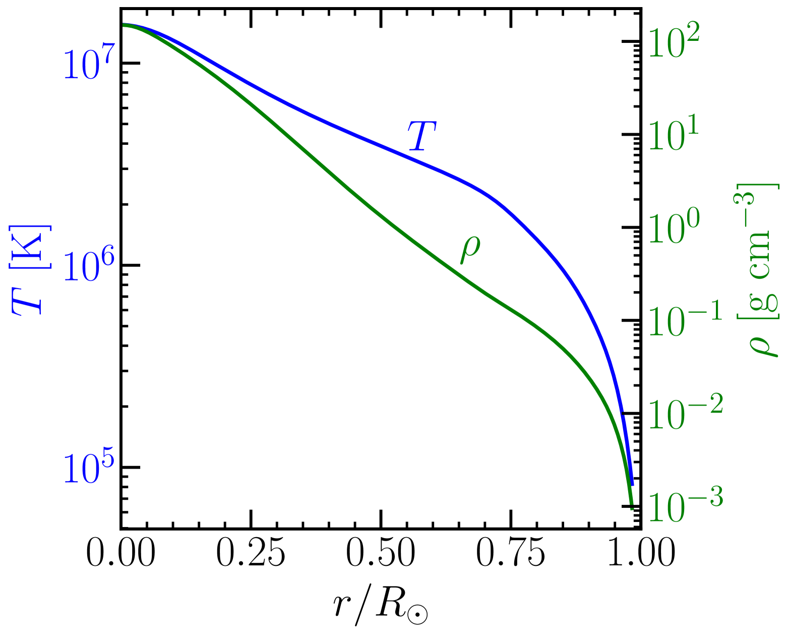
Figure 1: Density and temperature profiles from the reference solar model [67]. Note different y-axes.

The radial profile of the nuclear reaction rate density depends on the product of the number densities of the reactants, $n_{i}$, and the reaction rate factor, $\langle\sigma v\rangle$:

$$\Gamma_{ab}(r)=\frac{n_{a}n_{b}}{1+\delta_{ab}}\langle\sigma v\rangle,$$ (3)

where the Kronecker delta accounts for identical reactants. The number densities $n_{i}$ for various atomic species $i$ can be obtained by multiplying the mass density, $\rho$, by the mass fraction per species divided by the species mass, $X_{i}/m_{i}$. For $\langle\sigma v\rangle$, we use a weighted average, obtained by integration over the center-of-mass energy, $E$ (assuming a stationary target) of the product of the the fusion cross section, $\sigma(E)$, the velocity, $v(E)$, and the distribution of particles, $f(E)$, i.e.,

$$\langle\sigma v\rangle=\int_{0}^{\infty}dE\,\sigma(E)v(E)f(E).$$ (4)

The energy-dependent behavior in the cross section is typically encapsulated via the experimentally determined astrophysical S-factor, defined by

$$\sigma(E)=\frac{S(E)}{E}\exp\bigparenthesis{-\sqrt{\frac{E_{\mathrm{G}}}{E}}},$$ (5)

where $E_{G}=2m_{r}c^{2}(\pi\alpha Z_{a}Z_{b})^{2}$ is the Gamow energy in CGS units (fine structure constant $\alpha=e^{2}/\hbar c$, with the elementary charge $e$, reduced Planck constant $\hbar$, and speed of light $c$), $m_{r}$ is the reduced mass of the pair of reactants, and $Z_{i}$ are their atomic numbers. The exponential function in Eq. (5) is often written as $\exp\bigparenthesis{-2\pi\eta}$ (the Gamow factor), where $\eta=Z_{a}Z_{b}(e^{2}/h)\sqrt{m_{r}c^{2}/(2E)}$ is the Sommerfeld parameter with the Planck constant $h$. For a non-relativistic Maxwellian distribution of particles, the reaction rate factor is

$$\begin{split}\langle\sigma v\rangle&=\frac{2\sqrt{2}}{\sqrt{m_{r}\pi}}\frac{1}{(k_{B}T)^{3/2}}\\ &\times\int_{0}^{\infty}dE\,S(E)\exp\bigparenthesis{-\frac{E}{k_{B}T}-2\pi\eta},\end{split}$$ (6)

with the Boltzmann constant, $k_{\mathrm{B}}$.

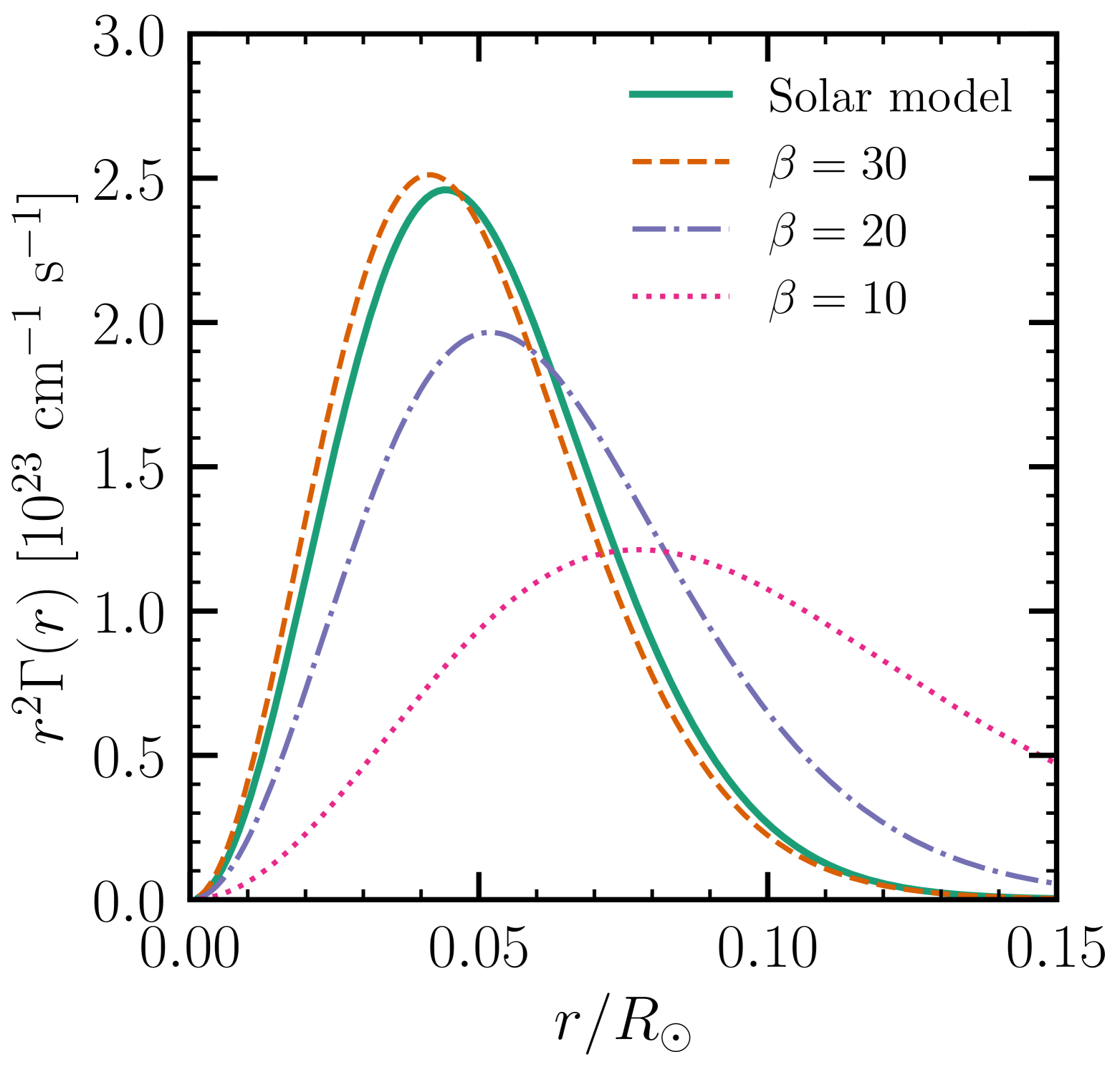
Figure 2: Full calculation of the ⁸B neutrino production rate profile compared to approximations that use only a simple scaling of the temperature profile. The normalizations of the latter curves are set equal to that of the full calculation.

At astrophysical energies ($k_{\mathrm{B}}T\approx 1.3$ keV in the solar core), $S(E)$ is usually (in the absence of nuclear resonances) a very slowly varying function. It is typical to write an effective S-factor, $S_{\mathrm{eff}}$, as Taylor series, for which coefficients are determined from theory and measurements. To describe reaction rates in the Sun, we use the compact approximation given in Ref. [4],

$$\begin{split}\langle\sigma v\rangle&=1.3005\times 10^{-15}\left[\frac{Z_{a}Z_{b}}{AT_{6}^{2}}\right]^{1/3}\\ &\times f_{0}S_{\mathrm{eff}}\exp(-\tau)\text{ cm}^{3}\text{ s}^{-1},\end{split}$$ (7)

where $A$ is the reduced mass of the two species in atomic mass units and $T_{6}=T/(10^{6}\text{ K})$. The factor

$$f_{0}=\exp\bigparenthesis{0.188Z_{a}Z_{b}\varphi\rho^{1/2}T_{6}^{-3/2}}$$ (8)

accounts for the screening of electrons, where $\rho$ is the mass density (in implicit units of g cm^-3) and $\varphi=\left[\sum_{i}(X_{i}Z_{i}^{2}/A_{i}+X_{i}Z_{i}/A_{i})\right]^{1/2}$. The latter quantity is usually labeled $\zeta$ in the literature, here we use $\varphi$ here to avoid confusion with a quantity connected with neutrino mixing (Sec. II.2). Next,

$$\begin{split}S_{\mathrm{eff}}&=S_{\mathrm{eff}}(E_{0})\approx S(0)\Biggl{[}1+\frac{5}{12\tau}+\frac{S^{\prime}}{S}\left(E_{0}+\frac{35}{36}k_{\mathrm{B}}T\right)\\ &+\frac{S^{\prime\prime}E_{0}}{S}\left(\frac{E_{0}}{2}+\frac{89}{72}k_{\mathrm{B}}T\right)\Biggr{]}_{E=0}\end{split}$$ (9)

is the effective astrophysical S-factor, where $E_{0}=1.2204\left(Z_{1}^{2}Z_{2}^{2}AT_{6}^{2}\right)^{1/3}\text{ keV}$ is the most probable energy of interaction (the Gamow peak), $\tau=3E_{0}/(k_{\mathrm{B}}T)=42.487\left(Z_{1}^{2}Z_{2}^{2}AT_{6}^{-1}\right)^{1/3}$ is a dimensionless parameter convenient for the power series expansion of the S-factor, where $S(E)$, $S^{\prime}\equiv dS/dE$, and $S^{\prime\prime}\equiv d^{2}S/dE^{2}$ are all evaluated at $E=0$. Recommendations for the S-factors can be found in reviews of solar fusion [20, 22, 24]. In the literature, the S-factor for the reaction in Eq. (1) is referred to as $S_{17}$. We use the central value recommended in Ref. [24] and neglect its uncertainties (see Sec. III.2). Finally, the factor $\exp(-\tau)$ arises from the Gamow peak.

Figure 2 shows our full calculation of the ⁸B neutrino production rate profile (which includes the geometrical factor of $r^{2}$ but not the angular factor of $4\pi$), following Eq. (3), where we take inputs from the reference solar model [67]. The neutrino production zone is defined by the radii where this function is large. We have checked that our calculation in the solid line closely matches the shape of the similar function in Ref. [67] (not shown).

Figure 2 also shows an important point: that the full profile can be well approximated by simply $\Gamma(r)\propto r^{2}T(r)^{\beta}$. This may be somewhat surprising, as the calculations above show that the temperature and density enter the calculations in multiple ways. To understand why this approximation works well, a few insights are needed. First, we can largely ignore the density dependence that appears in Eq. (3). In the radial range 0–0.1$R_{\odot}$, the number density of ¹H is only slightly falling and that of ⁷Be falls by about an order of magnitude. While the latter sounds important, it can be accommodated by a moderate increase in $\beta$, as shown in the figure. We find that the full calculation can be largely recovered by using $\beta\approx 27$.

Second, the reaction rate factor, $\langle\sigma v\rangle$, as specified in Eq. (7), can be taken to be independent of density and to depend on temperature primarily through the terms $\langle\sigma v\rangle\propto T(r)^{-2/3}\exp(-\tau)$. The variations in $f_{0}$ and $S_{\mathrm{eff}}$ with temperature and density are comparatively very weak. Then we can write

$$\langle\sigma v\rangle=\langle\sigma v\rangle_{0}\left(\frac{T(r)}{T_{0}}\right)^{\beta},\text{ }\beta=\frac{\partial\ln\langle\sigma v\rangle}{\partial\ln T(r)}$$ (10)

where $\langle\sigma v\rangle_{0}$ is a normalization factor and $T_{0}$ is some reference temperature [69]. Following straightforward algebraic manipulation, it can be shown that

$$\beta\approx\frac{\tau}{3}.$$ (11)

For the fusion of ⁷Be and a proton near the solar center, $\tau\approx 41$, so $\beta\approx 14$ is the expected value.

We must distinguish between two temperature exponents and how they are used. Above, $\beta$ is applied to the local temperature, $T(r)$. Separately, the total ⁸B neutrino flux scales as $T_{\textrm{c}}^{\alpha}$, where $T_{\textrm{c}}$ is the central temperature [70]. Across many contemporary solar models, it is found that $\alpha\approx 24\pm 5$ [65] (at the time of Ref. [4], it was said that $\alpha\approx 18$, which may be a more familiar value).

In lieu of developing our own self-consistent non-standard solar model, we exploit the fact that $\Gamma(r)\propto r^{2}T(r)^{\beta}$ to develop a semi-model-independent approach to probe the densities of the ⁸B production region. While a curve with $\beta\approx 14$ in Fig. 2 would be shifted to slightly larger radii than the full calculation, the width of the distribution is approximately correct. (We have checked that including the radial composition profiles for ¹H and especially ⁷Be leads to close agreement with the full calculation.) Therefore, as a first step towards a more sophisticated approach that will be possible with future data, we will assume that the uncertainties we derive with our approximate approach will be informative, even if the values are somewhat shifted.

As we show in Sec. II.2, varying $\beta$ changes the electron neutrino survival probability at Earth because it changes the density at production. To be conservative, we neglect the fact that varying $\beta$ would also change the total neutrino flux at Earth because it changes the temperature at production; instead, we keep the total flux at the central value measured by SNO. As discussed in Sec. III.2, in future work this effect can be taken advantage of.

II.2 Propagation

Neutrinos born in the electron-rich environment of the solar core experience flavor mixing due to the MSW effect. This mixing depends on three particle parameters, where we use the values taken from reactor experiments: $\tan^{2}(2\theta_{12})=0.436^{+0.102}_{-0.081}$, $\Delta m^{2}_{21}=(7.58\pm 0.21)\times 10^{-5}$ eV², and $\sin^{2}(\theta_{13})=0.032\pm 0.047$ [38, 71]. We quote the uncertainties to indicate their impressive precision, but neglect them in our calculation because we focus on the near-future situation in which they will be much smaller, following measurements by JUNO and other experiments. We use the mixing parameters from reactor experiments because they are independent of solar astrophysics; our results do not change much if we instead use the mixing parameters from solar experiments.

The first discussions of probing the solar density using neutrino mixing were in Refs. [59, 60], which considered the limits of large and small mixing angles, respectively. The physics of this problem for the LMAO case was developed further in Refs. [61, 62], which found best-fit densities in some tension with solar models. More recently, Refs. [63, 64] developed new statistical tools for this problem, finding overall compatibility with solar models. Our focus is on developing a more detailed approach with clearer physical and statistical insights, plus we also probe the solar temperature and develop the first joint probes for the $\rho,T$ plane (Sec. III).

Figure 3 shows how the mixing angle is modified in matter due to the MSW effect, the core idea of those studies. The matter angle $\theta$ depends on the solar electron number density as [72, 73]

$$\cos{(2\theta(E_{\nu},n_{\mathrm{e}}))}=\frac{-\phi}{\sqrt{\Lambda^{2}+\phi^{2}}}$$ (12)

where $\Lambda=\sin{(2\theta_{12})}$, $\phi=\zeta(E_{\nu},n_{\mathrm{e}})-\cos{(2\theta_{12})}$, and $\zeta=2\sqrt{2}G_{F}E_{\nu}n_{\mathrm{e}}/\Delta m^{2}_{21}$, with $E_{\nu}$ being the neutrino energy and $G_{F}$ being the Fermi coupling constant, and $n_{\mathrm{e}}$ is the number density of electrons. The electron number density profile, $n_{\mathrm{e}}(r)$, is related to the mass density, $\rho(r)$, via the mean molecular weight per electron, $\mu_{\mathrm{e}}(r)$. This final factor encodes the composition profiles from the reference solar model.

In vacuum, the matter mixing angle simply becomes the standard mixing angle, $\theta_{12}$. Note that ⁸B neutrino production occurs at small radii (Fig. 2), while the MSW resonances occur at moderate radii (Fig. 3). This turns out to be critical, as detailed below.

The three-flavor electron neutrino survival probability is approximately [74, 71, 75]

$$P_{\nu_{\mathrm{e}}}(E_{\nu})=\cos^{4}{(\theta_{13})}P_{2\nu_{\mathrm{e}}}(E_{\nu})+\sin^{4}{(\theta_{13})},$$ (13)

where we have neglected a small effect due to solar matter effects on $\theta_{13}$, and where the two-flavor component is

$$P_{2\nu_{\mathrm{e}}}(E_{\nu})=\frac{1}{2}\left[1+\langle\cos{(2\theta(E_{\nu}))}\rangle_{\mathrm{src}}\cos{(2\theta_{12})}\right].$$ (14)

The two factors in Eq. (14) reflect the initial and final matter angles, where the initial one must be averaged over the neutrino production rate profile and the final one is the same as in laboratory experiments. (To keep focus on the Sun, we neglect neutrino regeneration effects in Earth, which would increase the survival probability by a few percent in this energy range [76, 75].) Importantly, Eq. (13) depends only on the (averaged) matter density at ⁸B production, and not the densities along the neutrino trajectories.

Before discussing the validity and averaging of Eqs. (13, 14), we note some key physics points, building on Ref. [59]. The only place that the solar density appears is in the initial matter angle, $\cos{(2\theta(E_{\nu},n_{\mathrm{e}}))}$; this is also the only place that the neutrino energy appears. Consider three cases where observations of neutrino mixing would reveal nothing about the solar interior:

• If $\Delta m^{2}_{21}$ had been much larger (equivalent to the solar core densities or typical neutrino energies being much smaller — see the 1 MeV curve in Fig. 3 — or to having the MSW resonance density be much larger than the ⁸B production density), then $\cos{(2\theta(E_{\nu},n_{\mathrm{e}}))}\rightarrow\cos{(2\theta_{12})}$ and $P_{2\nu_{\mathrm{e}}}$ is a constant ($=\frac{1}{2}[1+\cos^{2}({2\theta_{12}})]$).

• If $\Delta m^{2}_{21}$ had been much smaller (equivalent to the opposite conditions), then $\cos{(2\theta(E_{\nu},n_{\mathrm{e}}))}\rightarrow-1$ and $P_{2\nu_{\mathrm{e}}}$ is a constant ($=\sin^{2}({\theta_{12}})$).

• If $\Delta m^{2}_{21}$ had been somewhat smaller and fine-tuned so that the MSW resonance density was equal to the ⁸B production density, then $\cos{(2\theta(E_{\nu},n_{\mathrm{e}}))}\rightarrow 0$ and $P_{2\nu_{\mathrm{e}}}$ is a constant ($=1/2$). There is a slight exception in this case, because some density dependence could arise through source averaging.

It is therefore fortunate that we are in the situation where ⁸B neutrino mixing via $\Delta m^{2}_{21}$ does probe the solar interior. Incidentally, the first bullet above is part of why mixing via the much larger $\Delta m^{2}_{31}$ is much less important (also, $\sin^{2}(\theta_{13})$ is small).

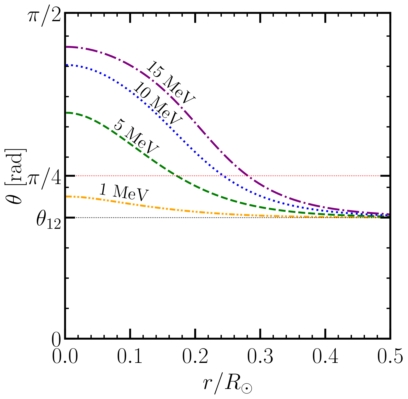
Figure 3: Variation of the matter angle throughout the Sun for three representative neutrino energies for ⁸B and one much lower energy for contrast. For a given neutrino energy, the MSW resonance occurs when the matter angle is $\pi/4$. That criterion and the vacuum mixing angle are noted with horizontal dotted lines.

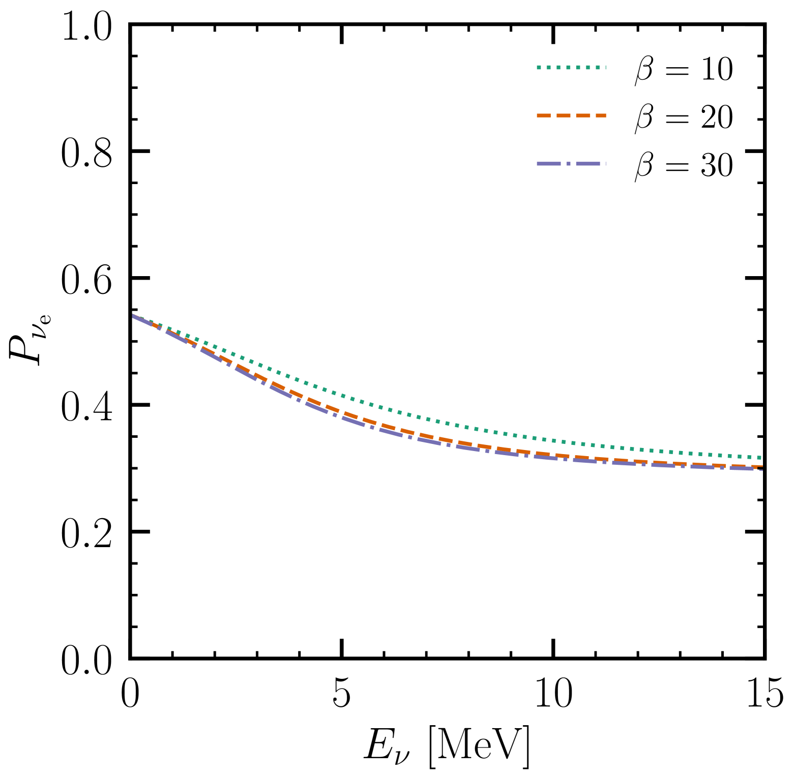
Figure 4: Electron neutrino survival probability at Earth as a function of neutrino energy for representative parameterizations of the neutrino production zone.

The form of the survival probability in Eqs. (13, 14) is valid under two conditions. First, the neutrino propagation must be adiabatic, meaning that the probability to jump from one mass eigenstate to another — which depends on the density along the neutrino trajectory — must be negligible, as it is for the LMAO mixing parameters [77, 73]. (For small mixing angles, in contrast, the survival probability can depend only on the density — more accurately, the variation of the density — along the neutrino trajectory [59, 60].) Second, we must be able to neglect oscillatory terms in the neutrino survival probability [72]. As part of this, we note that the neutrino oscillation length in matter,

$$L_{\mathrm{M}}^{\mathrm{osc}}=\frac{4\pi E}{\Delta m_{\mathrm{M}}^{2}},$$ (15)

should be negligible compared to the size of the neutrino production zone. The effective mass splitting is

$$\Delta m_{\mathrm{M}}^{2}=\Delta m_{21}^{2}\sqrt{(\cos{(2\theta_{12})}-\zeta)^{2}+\Lambda^{2}}.$$ (16)

The size of the neutrino production zone is of order $10^{-1}R_{\odot}$, while the oscillation length in matter of the most energetic solar neutrinos does not exceed $10^{-3}R_{\odot}$.

The initial-state cosine must be averaged over the ⁸B neutrino production zone as

$$\langle\cos{2\theta(E_{\nu},\beta)}\rangle_{\mathrm{src}}=\int_{r_{\mathrm{min}}}^{r_{\mathrm{max}}}dr\,r^{2}T(r)^{\beta}\cos\left(2\theta(E_{\nu},n_{\mathrm{e}})\right),$$ (17)

where the neutrino production rate profile, which is proportional to $r^{2}T(r)^{\beta}$, is normalized to unity for use in the above integral (the normalization is taken into account in Sec. II.3). As shown above, it is a reasonable approximation to characterize the neutrino production rate profile in this way, neglecting smaller effects due to the radial variation of density and composition.

Figure 4 shows the electron neutrino survival probability as a function of neutrino energy for representative neutrino production zones. For the electron number density profile from the reference solar model, the largest differences in survival probability for different neutrino production zones occur in the intermediate energy range, around 3–8 MeV. Even so, it is difficult to distinguish between the deepest production zones, e.g., the highest values of $\beta$. This is due to the flattening of the $n_{\mathrm{e}}$ profile in the core. That means that even though the $\beta=30$ and $\beta=20$ cases look different in Fig. 2, they are hard to distinguish with ⁸B neutrinos.

We close with another important point. In Eqs. (13, 14), the solar density dependence is tied to the neutrino energy dependence. However, this does not mean that measuring the energy dependence of the survival probability would allow us to invert for the radial density profile. At each neutrino energy, a range of radii in the neutrino production zone contribute, but only the average survival probability can be probed. If the ⁸B neutrino production zone were narrower in radius, the differences shown in Fig. 4 would be larger. Even so, appreciable differences remain.

II.3 Detection

For ⁸B neutrinos, we focus on observations with Super-K, due to their high statistics and broad spectrum coverage [66]. There are also observations with SNO [78] and Borexino [79]. Super-K, located deep underground in Japan, is a water-Cherenkov neutrino detector sensitive to MeV-scale neutrinos. It has a fiducial volume of 22.5 kton. Neutrinos from the Sun elastically scatter with electrons in the water via both charged- and neutral-current interactions. The spectrum of recoil electrons can be predicted using the neutrino production and propagation calculations above, the physics of weak interactions, and detector effects.

It is important to note that Super-K (and Borexino) do not directly measure the electron neutrino survival probability. (Below, we discuss the potential of using SNO’s charged-current neutrino-deuteron data.) First, because the differential cross section for neutrino-electron scattering is broad, measurements can be made only as a function of electron energy, not neutrino energy. Second, as discussed below, the non-electron-neutrino flavors contribute at a small level to the observed data. Third, in order to normalize expectations in a semi-model-independent way, they rely on SNO’s measurement of the total flux via neutral-current neutrino-deuteron interactions; this is only available for ${}^{\textit{8}}$B neutrinos. Finally, just as a point of presentation, Super-K typically shows the ratio of the observed recoil electron spectrum to its theoretical expectation (relatively flat), rather than the recoil electron spectrum itself (relatively steep).

We begin with the initial electron spectrum,

$$R(\mathcal{T})=\int_{\mathrm{E}_{\nu}^{\mathrm{min}}}^{\mathrm{E}_{\nu}^{\mathrm{max}}}d\mathrm{E}_{\nu}\ \Phi_{\nu}(\mathrm{E}_{\nu})\mathcal{P}(\mathcal{T},\mathrm{E}_{\nu}),$$ (18)

where $\mathcal{T}$ is the true (before energy resolution effects) electron kinetic energy, $\mathrm{E}_{\nu}^{\mathrm{min}}=\frac{1}{2}\left(\mathcal{T}+\sqrt{\mathcal{T}^{2}+2m_{\mathrm{e}}/\mathcal{T}}\right)$ is given by kinematics with the electron mass $m_{\mathrm{e}}$, and $\mathrm{E}_{\nu}^{\mathrm{max}}$ is the cutoff of the neutrino energy spectrum. The differential solar neutrino flux,

$$\Phi_{\nu}(\mathrm{E}_{\nu})=\phi_{\mathrm{tot}}\mathrm{f}(\mathrm{E}_{\nu}),$$ (19)

is defined by $\phi_{\mathrm{tot}}=(5.25\pm 0.20)\times 10^{6}\text{ cm}^{-2}\text{ s}^{-1}$ which is the total ⁸B neutrino flux measured by SNO [36], and $\mathrm{f}(\mathrm{E}_{\nu})$ which is the ⁸B neutrino energy spectrum [68].

Neutrino oscillations and elastic scattering are accounted for via

$$\begin{split}\mathcal{P}(\mathcal{T},\mathrm{E}_{\nu})&=\biggl{[}P_{\nu_{\mathrm{e}}}(\mathrm{E}_{\nu})\frac{d\sigma_{e}}{d\mathcal{T}}(\mathcal{T},\mathrm{E}_{\nu})\\ &+\left(1-P_{\nu_{\mathrm{e}}}(\mathrm{E}_{\nu})\right)\frac{d\sigma_{\mu}}{d\mathcal{T}}(\mathcal{T},\mathrm{E}_{\nu})\biggr{]},\end{split}$$ (20)

where $P_{\nu_{\mathrm{e}}}(\mathrm{E}_{\nu})$ is the survival probability of electron neutrinos as a function of neutrino energy as given in Eq. (13) and $d\sigma_{\chi}/d\mathcal{T}(\mathcal{T},\mathrm{E}_{\nu})$ is the differential cross section [80]. Here, $\chi$ is $\mathrm{e}$ or $\mu/\tau$ for the electron and muon/tau flavors. Because the latter two flavors do not have charged-current interactions with electrons, their differential cross section is $\approx$6 times lower than for electron neutrinos.

To account for energy resolution effects in Super-K, Eq. (18) is passed into

$$S(\mathcal{T})=\int_{{T_{\mathrm{e,min}}}}^{{T_{\mathrm{e,max}}}}dT_{\mathrm{e}}\ G(T_{\mathrm{e}},\mathcal{T},\sigma(\mathcal{T}))R(\mathcal{T}),$$ (21)

where $T_{\mathrm{e}}$ is the measured kinetic energy. The energy resolution is taken into account via Gaussian smearing [81],

$$\begin{split}G(T_{\mathrm{e}},\mathcal{T},\sigma(\mathcal{T}))&=\frac{1}{\sigma(\mathcal{T})\sqrt{2\pi}}\\ &\times\exp\left[-\frac{(\mathcal{T}-T_{\mathrm{e}})^{2}}{2(\sigma(\mathcal{T}))^{2}}\right],\end{split}$$ (22)

where

$$\begin{split}\sigma(\mathcal{T})&=-0.5525+0.3162\sqrt{\mathcal{T}+\mathrm{m}_{\mathrm{e}}}\\ &+0.04572(\mathcal{T}+m_{\mathrm{e}})\end{split}$$ (23)

models the energy resolution during the full Super-K-IV period [66]. The limits of integration in Eq. (21) are chosen to eliminate energy-resolution-induced smoothing effects on the edges of the spectrum.

Finally, the spectrum is discretized according to Super-K’s data bins as $\left(\Delta N/\Delta T\right)_{i}$, the event rate in the $i^{\text{th}}$ bin, in units of event day^-1 (22.5 kton)^-1 MeV^-1. We compute the final spectrum using

$$\left(\frac{\Delta N}{\Delta T}\right)_{i}=\frac{\mathrm{N}_{\mathrm{e}}}{\mathrm{M}_{\mathrm{det}}\Delta T_{i}}\int_{T_{i}^{\mathrm{left}}+\delta}^{T_{i}^{\mathrm{left}}+\Delta T_{i}+\delta}d\mathcal{T}\ S(\mathcal{T}),$$ (24)

where $\Delta T_{i}$ is the width of the $i^{\mathrm{th}}$ Super-K kinetic energy bin, $T_{i}^{\mathrm{left}}$ is the left edge of the bin, and $\delta$ is the uncertainty in the absolute energy scale of the detector [82], which we set to zero for simplicity. The prefactors outside the integral include $\mathrm{N}_{\mathrm{e}}=7.521\times 10^{33}$ as the number of electrons and $\mathrm{M}_{\mathrm{det}}=22.5$ kton as the total mass of water in Super-K’s fiducial volume.

In our calculations, we consider only the signal from ⁸B neutrinos. Those from the hep reaction are produced somewhat further out in the Sun ($\approx$$0.15R_{\odot}$) [83] and their spectrum extends to higher neutrino energies ($E_{\nu}^{\mathrm{max}}\approx 19$ MeV for $hep$ [84] compared to $E_{\nu}^{\mathrm{max}}\approx 15$ MeV for ⁸B). While hep neutrinos may be helpful in the future to study the solar interior, their contribution to the Super-K data is not yet detected. We thus exclude the last three Super-K bins, covering 13.49–19.49 MeV. Additionally, we consider only statistical uncertainties on the Super-K observed recoil electron spectrum. Energy-correlated systematic uncertainties become significant only in the highest-energy bins [66], which we have cut from our analysis. Energy-uncorrelated systematics are comparable to statistical uncertainties below $\approx$8 MeV. We have checked that these choices do not significantly impact our results.

We compare the results of our simple treatment to the Super-K collaboration’s careful Monte Carlo model of their detector (in the absence of neutrino mixing). For this case, the choice of $\beta$ does not enter ($P_{\nu_{\mathrm{e}}}(\mathrm{E}_{\nu})=1$). We first take the “day” observed rate from Table IX of Ref. [66]. We compare our numerical evaluation in Eq. (24) to the expected event rate in Super-K due to ⁸B neutrinos from the same table, and divide the observed rate by each model. Our calculation (detailed in the GitHub repository) is consistent with the Super-K model within their statistical uncertainties.

Figure 5 (top panel) shows our predictions for the spectrum of scattered electrons from Eq. (21) (with and without neutrino flavor mixing), compared to Super-K observations. The data points are a ratio between the observed spectrum in Super-K (with mixing implied) and their model (no mixing). Error bars show statistical uncertainties only. The upturn in the survival probability with decreasing neutrino energy (Fig. 4) becomes harder to observe in the electron ratio spectrum, e.g., the $\beta=30$ and $\beta=20$ cases are even harder to distinguish than they were in Fig. 4. Figure 5 (bottom panel) shows that our prediction of the electron spectrum accurately reproduces the Super-K observation, which is an important check.

III Calculation of probes of the solar core

In this section, we present our main results, which are the projected uncertainties in the density-temperature plane probed by ⁸B observations, referring to the best-fit values as $\rho_{\textrm{npz}}$ and $T_{\textrm{npz}}$ because neutrinos probe the values in the neutrino production zone. The density is probed via the neutrino survival probability and the temperature is probed by the flux. We then outline paths toward model-independent neutrino probes of the Sun.

III.1 Constraints in the $\rho,T$ plane

To probe the typical density for ⁸B production, we use $\beta$ to parameterize the shape of the neutrino production zone and hence the neutrino survival probability. We fit for $\beta$ by optimizing the log-likelihood,

$$\mathcal{L}(\beta)=-\frac{1}{2}\sum_{i}\left[\left(\frac{O_{i}-\left(\Delta N/\Delta T\right)_{i}(\beta)}{\sigma_{i}}\right)^{2}+\ln(2\pi\sigma_{i}^{2})\right],$$ (25)

where $O_{i}$ is the observed recoil electron spectrum in Super-K [66], the second term in the quadratic is the predicted spectrum using Eq. (24), and $\sigma_{i}$ are the statistical uncertainties.

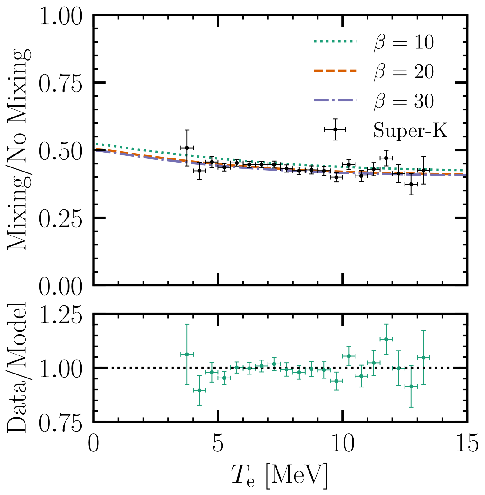
Figure 5: Top panel: Predictions of the electron spectrum for different $\beta$ values, calculated by taking the ratio of Eq. (21) with and without neutrino flavor mixing (see text). Bottom panel: Ratio between the Super-K observations [66] of the recoil electron spectrum and our prediction from Eq. (24) with neutrino flavor mixing, using $\beta=15$ as a representative case.

Figure 6 shows the resulting probability distribution for $\beta$. We obtain this by stepping over Eq. (25) for varying $\beta$ and plotting the Gaussian likelihood (via $\exp({\mathcal{L}(\beta)})$, normalized to unity). For small values of $\beta$, the distribution has a short tail because decreasing $\beta$ corresponds to moving the neutrino production zone to larger radii, thus smaller densities (Fig. 1), smaller matter angles (Fig. 3), and larger survival probabilities (Fig. 4), which would conflict with Super-K data (Fig. 5). For large values of $\beta$, the distribution has a long tail because increasing $\beta$, which leads to the opposites of the changes noted above, is less restricted. That is because the survival probability becomes flatter in Super-K’s energy range, in part because the solar density profile flattens out at small radii. Additionally, for smaller $\beta$, the distribution in Fig. 1 becomes narrower, so that the effects of averaging over the neutrino production zone in Eq. (17) are less.

Figure 7 shows the neutrino production rate profile corresponding to the best-fit value of beta. We find $17.2^{+5.0}_{-2.8}$, which is in agreement with the expectation of $\beta\approx 14$ that followed from semi-model-independent approach of approximating $\Gamma(r)\propto r^{2}T(r)^{\beta}$. This value of $\beta$ is lower than the value we find in a full calculation ($\beta\approx 27$, as shown in Fig. 2), but it is adequate for our purposes. Though the best-fit neutrino production rate profile is somewhat shifted compared to that of the full calculation, the widths of the distributions are comparable. The shift in the peak value from $\approx$$0.045R_{\odot}$ to $\approx$$0.055R_{\odot}$ corresponds to decreasing the density by $\approx$6%, corresponding to changes in the electron neutrino survival of $\lesssim 1\%$.

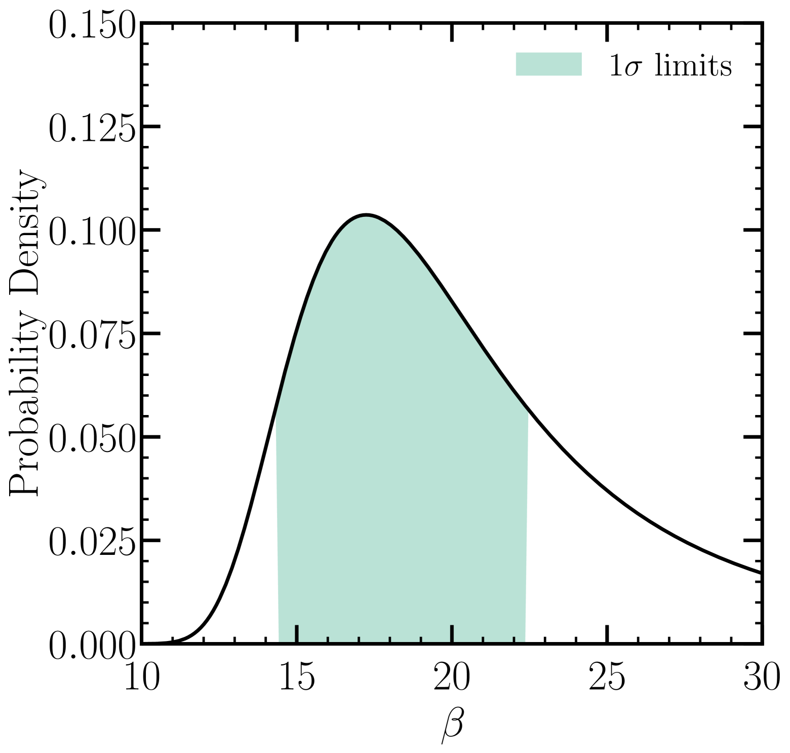
Figure 6: Probability density for $\beta$ given Super-K’s observed recoil electron spectrum. The best fit is $\beta=17.2^{+5.0}_{-2.8}$, where the uncertainties correspond to 68% of samples (with $34\%$ of samples on each side of the maximum).

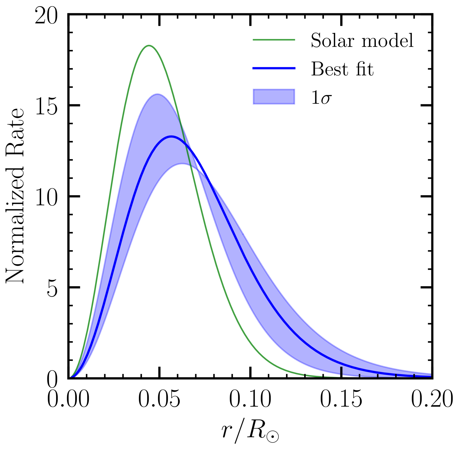
Figure 7: Neutrino production rate profile determined by our fit compared to that from the full calculation using the reference solar model. While our result is shifted relative to the full calculation, the width is similar.

To probe the typical temperature for ⁸B production, some assumptions are needed. As described in Sec. II.1, it has been found that the total ⁸B neutrino flux scales as $\phi_{\mathrm{tot}}\propto T_{\textrm{c}}^{24}$, where $T_{\textrm{c}}$ is the core temperature. What we need is a scaling relation in terms of $T_{\textrm{npz}}$, including the prefactor, determined from contemporary solar models. This does not seem to exist. To proceed, we assume the same exponent holds for $T_{\textrm{npz}}$, which is only 6% less than $T_{\textrm{c}}$ in the reference solar model. That is, we use $\phi_{\mathrm{tot}}\propto T_{\textrm{npz}}^{24}$, though the prefactor is unknown. While this does not allow us to directly extract the value of $T_{\textrm{c}}$ from the SNO measurement of the total ⁸B flux, it does allow us to approximate the projected uncertainty, which is our goal. Simple error propagation leads to $\delta\phi_{\mathrm{tot}}/\phi_{\mathrm{tot}}=24~\delta T_{\textrm{npz}}/T_{\textrm{npz}}$, where $\delta\phi_{\mathrm{tot}}$ and $\delta T_{\textrm{npz}}$ are the uncertainties on the total flux and the temperature in the neutrino production zone. We use $\delta\phi_{\mathrm{tot}}/\phi_{\mathrm{tot}}\approx 0.038$ from SNO [36].

Figure 8 shows our main results. As far as we are aware, this is the first time that joint neutrino probes of the solar interior density and temperature have been shown. For $\rho_{\textrm{npz}}$ and its uncertainty, we use the peak and width from Fig. 7, where we specify the latter by including 68% of the distribution, with 34% on each side of the maximum. This leads to $\rho_{\textrm{npz}}=121^{+19}_{-26}$ g cm^-3; in the reference solar model, this corresponds to the range of $0.031\leq r/R_{\odot}\leq 0.089$. Note that while we only use the MSW effect and the Super-K electron energy spectrum, we are able to constrain the radial range (and thus angular extent) of the neutrino production zone even without angular information. (Eventually, direct angular measurements may be possible [85].) For $T_{\textrm{npz}}$ and its uncertainty, we use the value from the reference solar model at the peak of the best-fit production profile and the uncertainty estimated above. We find $\delta T_{\textrm{npz}}/T_{\textrm{npz}}\approx 0.002$, or $T_{\textrm{npz}}=(1.453\pm 0.002)\times 10^{7}$ K.

Figure 8 also shows that neutrinos provide a unique perspective on the Sun, as they probe the deep interior of the Sun, which nothing else can do. Astronomical observations in the optical and other wavebands first probe the exterior of the Sun. With helioseismology, it is possible to probe the solar interior, though not this deep, and less directly, as the primary observable is the sound speed squared. Figure 8 (top panel) shows that even though neutrino observations are difficult, they are surprisingly powerful. Figure 8 (bottom panel) highlights the regions of the solar interior that can be probed. Overall, we find no evidence for significant problems in the physical description of the Sun.

III.2 Towards broader studies

As discussed in Sec. I, we are approaching a time when we can probe the astrophysics of the Sun in powerful new ways. Neutrinos are a unique tool for revealing the physical conditions of the solar interior, but their properties have been uncertain. With coming laboratory measurements of neutrino mixing, that uncertainty will be greatly reduced. In addition, there are excellent prospects for laboratory measurements and computational studies of the basic physics of nuclear reactions and atomic opacities to reduce those input uncertainties. For example, most of the error budget in the theoretical prediction of the total ⁸B flux lies in $S_{17}$. Even so, uncertainties on $S_{17}$ are about $\approx$3% [24], but will become even smaller via efforts in nuclear theory and experiment. These changes mean that we can focus our attention on things that can only be measured with solar data.

A theme illustrated by our work is that a true inversion from neutrino observations to solar-core parameters is not possible, even in the simplified calculations above. First, there are multiple steps that introduce significant smearing. Second, and more fundamentally, the Sun is an enormously complicated system with many variables. It only makes sense to consider changes to the solar core density and temperature that are consistent with the equations of stellar structure and wide variety of observational constraints. Therefore, one should consider the forward problem, where uncertain physical aspects of solar models are varied and their effects are carried through to neutrino and electromagnetic observables. This kind of approach can help address longstanding mysteries about the Sun.

For instance, there is discrepancy between heavy element abundances in the solar photosphere [44, 45, 46] and those in the interior implied from helioseismology [40, 41, 42]. Though much work has been done to study this tension using neutrinos [86, 87, 88], a solution to the solar metallicity problem has yet to be found. Other questions about solar models remain, for example, changing the compositions in the solar interior or sufficiently perturbing the microphysics [89, 90]. Specifically, the effects of including chemical mixing in the radiative zone via rotation or waves in solar models have yet to be explored.

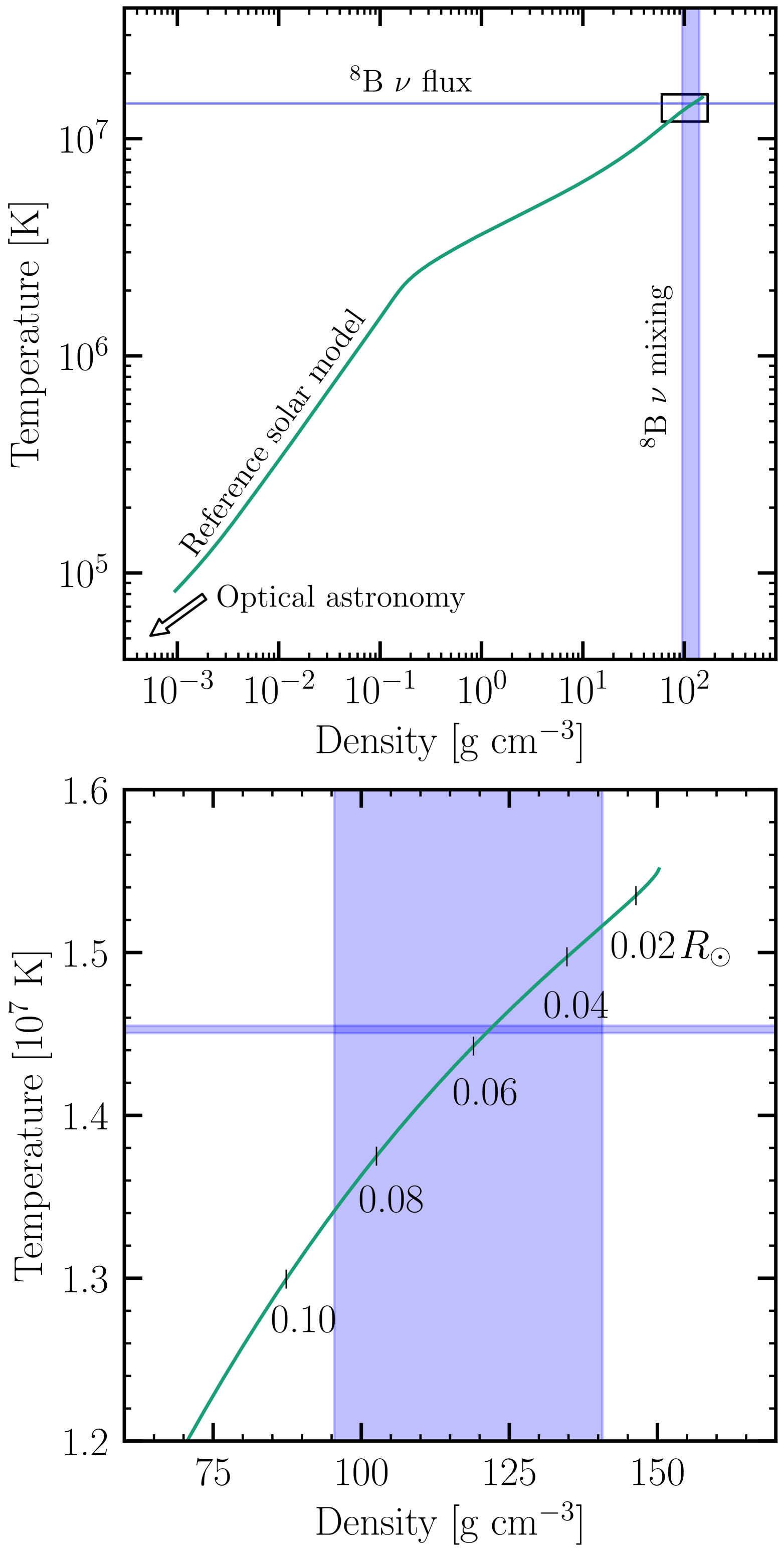
Figure 8: Our constraints on the reference solar model density and temperature profiles using ⁸B neutrino observations.

What is needed is for solar modelers to create large suites of models that sample over uncertainties in solar astrophysics. Decades ago, large suites of solar models were created by varying inputs via Monte Carlo [65]. However, given the computational constraints of the time, these models had to be characterized in simple ways, e.g., via scatterplots of the neutrino flux from one nuclear reaction versus another. It is now possible that the complete models could be shared. Or the solar modelers could collaborate with neutrino experimentalists and phenomenologists to accurately test which models actually remain allowed. In this way, the neutrino data would probe solar astrophysics in new ways.

In the future, there will also be better observations to test these phenomena. On the neutrino side, these observables include the fluxes and spectra of neutrinos from several different nuclear reactions, which have different sensitivities to changes in the physical conditions of their production zones. For example, better measurements of the pp neutrino flux would improve constraints on the Sun’s luminosity [91]. JUNO is poised to make improved measurements of ⁷Be, hep, and CNO neutrinos [92], which, in addition to ⁸B  [93, 57], would be helpful in addressing the solar metallicity problem [46]. Newly precise measurements of ⁸B solar neutrinos can also be made by Hyper-Kamiokande [49, 50] and DUNE [56, 94, 58]. Measurements of ⁸B neutrinos at as low energies as possible would help observe the upturn in the survival probability (Fig. 4). To make these ⁸B measurements as precise as possible, it would be important to reduce detector backgrounds even further [95, 96]. Studying the conditions of the solar core using neutrinos from pep and ⁷Be will require high precision because these lower-energy neutrinos experience weak matter effects (Fig. 3) as they are born at densities below the MSW resonance. The first measurements of the hep neutrino flux and spectrum would confirm that the rare pp-IV chain does indeed occur in the Sun and open the door to studying a different radial range inside the Sun around $\sim$$0.15R_{\odot}$. On the electromagnetic side, the primary need is for new efforts in helioseismology theory to better understand existing observations [97, 98].

Our analysis of ⁸B neutrinos could be improved. With varying solar models as described above, one could make direct calculations of their compatibility with ⁸B data. In this paper, we generate constraints on $\rho_{\textrm{npz}}$ and $T_{\textrm{npz}}$ separately. We took this approach because it is both semi-solar-model-independent and simple. By assuming the SNO measurement for $\phi_{\mathrm{tot}}$ and using $\Gamma(r)\propto r^{2}T(r)^{\beta}$, we conservatively ignored changes in the ⁸B flux; taking those into account would give greater sensitivity. Separately, it would be interesting to consider the charged-current neutrino-deuteron data from SNO, as the differential cross section is narrower and only electron neutrinos contribute, though the statistics are lower.

IV Conclusions and Outlook

At present, solar neutrinos are not receiving as much attention as they did in earlier decades. This isn’t because we ran out of questions — it’s because we ran out of data. In the next decade, this will change significantly, as JUNO, Hyper-Kamiokande, DUNE, and other experiments (e.g., possibly XLZD [99]) come online. Those experiments will make much more precise measurements of solar neutrino fluxes and spectra. And, because these and other experiments will also make much more precise measurements of neutrino mixing parameters through independent measurements of laboratory neutrino sources, we have new opportunities to use solar neutrinos to probe the astrophysics of the solar interior.

Even with present solar-neutrino data, there will be important steps that can be taken once the neutrino mixing parameters are better known. Building on Refs. [4, 65], we show that the total flux of ⁸B neutrinos measured by SNO probes the temperature of the neutrino production zone, $T_{\textrm{npz}}$. Building on Refs. [59, 60, 61, 62, 63, 64], we show that the oscillated flux of ⁸B neutrinos measured by Super-K probes the density of the neutrino production zone, $\rho_{\textrm{npz}}$. Last, we are the first to combine these to obtain projected joint constraints on the density-temperature plane. Using straightforward treatments of neutrino production, propagation, and detection, we show that we can expect to obtain tight constraints in that plane with only minor reliance on solar models.

Quoting from Bahcall’s 1964 paper [16], “Only neutrinos, with their extremely small interaction cross sections, can enable us to see into the interior of a star and thus verify directly the hypothesis of nuclear energy generation in stars.” More than sixty years later, this dream is within reach. Neutrinos take patience, but they reward it richly.

The Python code used to generate our results and the figures in this paper, as well as the relevant data files, are all available on GitHub.

Note added: In the final stages of preparing our paper, there appeared a new paper (Ref. [100]) that addresses similar directions but with a different approach and complementary results.

References

- Fowler [1958] W. A. Fowler, Completion of the Proton-Proton Reaction Chain and the Possibility of Energetic Neutrino Emission by Hot Stars., Astrophys. J. 127, 551 (1958).
- Bahcall et al. [1963] J. N. Bahcall, W. A. Fowler, J. Iben, I., and R. L. Sears, Solar Neutrino Flux., Astrophys. J. 137, 344 (1963).
- Sears [1964] R. L. Sears, Helium Content and Neutrino Fluxes in Solar Models, Astrophys. J. 140, 477 (1964).
- Bahcall [1989] J. N. Bahcall, Neutrino Astrophysics (Cambridge University Press, 1989).
- Rolfs and Rodney [1988] C. E. Rolfs and W. S. Rodney, Cauldrons in the cosmos : nuclear astrophysics (University of Chicago Press, 1988).
- Davis et al. [1968] R. Davis, Jr., D. S. Harmer, and K. C. Hoffman, Search for neutrinos from the sun, Phys. Rev. Lett. 20, 1205 (1968).
- Hirata et al. [1989] K. S. Hirata et al. (Kamiokande-II), Observation of B-8 Solar Neutrinos in the Kamiokande-II Detector, Phys. Rev. Lett. 63, 16 (1989).
- Abazov et al. [1991] A. I. Abazov et al., First results from the Soviet-American gallium experiment, Nucl. Phys. B Proc. Suppl. 19, 84 (1991).
- Anselmann et al. [1992] P. Anselmann et al. (GALLEX), Implications of the GALLEX determination of the solar neutrino flux., Phys. Lett. B 285, 390 (1992).
- Fukuda et al. [1998] Y. Fukuda et al. (Super-Kamiokande), Measurements of the solar neutrino flux from Super-Kamiokande’s first 300 days, Phys. Rev. Lett. 81, 1158 (1998), [Erratum: Phys.Rev.Lett. 81, 4279 (1998)], arXiv:hep-ex/9805021 .
- Ahmad et al. [2001] Q. R. Ahmad et al. (SNO), Measurement of the rate of interactions produced by 8B solar neutrinos at the Sudbury Neutrino Observatory, Phys. Rev. Lett. 87, 071301 (2001), arXiv:nucl-ex/0106015 .
- Anderson et al. [2019] M. Anderson et al. (SNO+), Measurement of the 8B solar neutrino flux in SNO+ with very low backgrounds, Phys. Rev. D 99, 012012 (2019), arXiv:1812.03355 [hep-ex] .
- Ma et al. [2023] W. Ma et al. (PandaX), Search for Solar B8 Neutrinos in the PandaX-4T Experiment Using Neutrino-Nucleus Coherent Scattering, Phys. Rev. Lett. 130, 021802 (2023), arXiv:2207.04883 [hep-ex] .
- Aprile et al. [2024] E. Aprile et al. (XENON), First Indication of Solar B8 Neutrinos via Coherent Elastic Neutrino-Nucleus Scattering with XENONnT, Phys. Rev. Lett. 133, 191002 (2024), arXiv:2408.02877 [nucl-ex] .
- Bahcall et al. [1963] J. N. Bahcall, W. A. Fowler, I. Iben, Jr., and R. L. Sears, Solar neutrino flux, Astrophys. J. 137, 344 (1963).
- Bahcall [1964] J. N. Bahcall, Solar neutrinos. I: Theoretical, Phys. Rev. Lett. 12, 300 (1964).
- Davis [1964] R. Davis, Solar neutrinos. II: Experimental, Phys. Rev. Lett. 12, 303 (1964).
- Cox and Stewart [1970] A. N. Cox and J. N. Stewart, Rosseland Opacity Tables for Population i Compositions, Astrophysical Journal Supplement 19, 243 (1970).
- Seaton [1987] M. J. Seaton, Atomic data for opacity calculations. I. General description, Journal of Physics B Atomic Molecular Physics 20, 6363 (1987).
- Adelberger et al. [1998] E. G. Adelberger et al., Solar fusion cross-sections, Rev. Mod. Phys. 70, 1265 (1998), arXiv:astro-ph/9805121 .
- Däppen and Guzik [2000] W. Däppen and J. A. Guzik, Astrophysical Equation of State and Opacity, in Variable Stars as Essential Astrophysical Tools, NATO Advanced Study Institute (ASI) Series C, Vol. 544, edited by C. Ibanoglu (2000) p. 177.
- Adelberger et al. [2011] E. G. Adelberger et al., Solar fusion cross sections II: the pp chain and CNO cycles, Rev. Mod. Phys. 83, 195 (2011), arXiv:1004.2318 [nucl-ex] .
- Pain et al. [2017] J.-C. Pain, F. Gilleron, and M. Comet, Detailed Opacity Calculations for Astrophysical Applications, Atoms 5, 22 (2017), arXiv:1706.01761 [astro-ph.SR] .
- Acharya et al. [2024] B. Acharya et al., Solar fusion III: New data and theory for hydrogen-burning stars, Reviews of Modern Physics (2024), arXiv:2405.06470 [astro-ph.SR] .
- Chandrasekhar [1939] S. Chandrasekhar, An introduction to the study of stellar structure (The University of Chicago Press, 1939).
- Henyey et al. [1964] L. G. Henyey, J. E. Forbes, and N. L. Gould, A New Method of Automatic Computation of Stellar Evolution., Astrophys. J. 139, 306 (1964).
- Cox and Giuli [1968] J. P. Cox and R. T. Giuli, Principles of stellar structure (Gordon and Breach, Science Publishers, Inc, 1968).
- Clayton [1983] D. D. Clayton, Principles of stellar evolution and nucleosynthesis (McGraw-Hill, 1983).
- Hansen and Kawaler [1994] C. J. Hansen and S. D. Kawaler, Stellar Interiors. Physical Principles, Structure, and Evolution. (Springer-Verlag, 1994).
- Kippenhahn et al. [2013] R. Kippenhahn, A. Weigert, and A. Weiss, Stellar Structure and Evolution (Springer, 2013).
- Serenelli [2016] A. Serenelli, Alive and well: a short review about standard solar models, Eur. Phys. J. A 52, 78 (2016), arXiv:1601.07179 [astro-ph.SR] .
- Christensen-Dalsgaard [2021] J. Christensen-Dalsgaard, Solar structure and evolution, Living Reviews in Solar Physics 18, 2 (2021), arXiv:2007.06488 [astro-ph.SR] .
- Pontecorvo [1967] B. Pontecorvo, Neutrino Experiments and the Problem of Conservation of Leptonic Charge, Zh. Eksp. Teor. Fiz. 53, 1717 (1967).
- Wolfenstein [1978] L. Wolfenstein, Neutrino Oscillations in Matter, Phys. Rev. D 17, 2369 (1978).
- Mikheev and Smirnov [1986] S. P. Mikheev and A. Y. Smirnov, Resonant amplification of neutrino oscillations in matter and solar neutrino spectroscopy, Nuovo Cim. C 9, 17 (1986).
- Aharmim et al. [2013] B. Aharmim et al. (SNO), Combined Analysis of all Three Phases of Solar Neutrino Data from the Sudbury Neutrino Observatory, Phys. Rev. C 88, 025501 (2013), arXiv:1109.0763 [nucl-ex] .
- Eguchi et al. [2003] K. Eguchi et al. (KamLAND), First results from KamLAND: Evidence for reactor anti-neutrino disappearance, Phys. Rev. Lett. 90, 021802 (2003), arXiv:hep-ex/0212021 .
- Abe et al. [2008] S. Abe et al. (KamLAND), Precision Measurement of Neutrino Oscillation Parameters with KamLAND, Phys. Rev. Lett. 100, 221803 (2008), arXiv:0801.4589 [hep-ex] .
- Gando et al. [2013] A. Gando et al. (KamLAND), Reactor On-Off Antineutrino Measurement with KamLAND, Phys. Rev. D 88, 033001 (2013), arXiv:1303.4667 [hep-ex] .
- Basu and Antia [2008] S. Basu and H. M. Antia, Helioseismology and Solar Abundances, Phys. Rept. 457, 217 (2008), arXiv:0711.4590 [astro-ph] .
- van Saders and Pinsonneault [2012] J. L. van Saders and M. H. Pinsonneault, The Sensitivity of Convection Zone Depth to Stellar Abundances: An Absolute Stellar Abundance Scale from Asteroseismology, Astrophys. J. 746, 16 (2012), arXiv:1108.2273 [astro-ph.SR] .
- Christensen-Dalsgaard [2019] J. Christensen-Dalsgaard, Helioseismology and solar neutrinos, in 5th International Solar Neutrino Conference (2019) pp. 81–102, arXiv:1809.03000 [astro-ph.SR] .
- Buldgen et al. [2025] G. Buldgen, J.-C. Pain, P. Cossé, C. Blancard, F. Gilleron, A. Pradhan, C. J. Fontes, J. Colgan, A. Noels, J. Christensen-Dalsgaard, M. Deal, S. V. Ayukov, V. A. Baturin, A. V. Oreshina, R. Scuflaire, C. Pinçon, Y. Lebreton, T. Corbard, P. Eggenberger, P. Hakel, and D. P. Kilcrease, Helioseismic inference of the solar radiative opacity, arXiv e-prints , arXiv:2504.06891 (2025), arXiv:2504.06891 [astro-ph.SR] .
- Bergemann and Serenelli [2014] M. Bergemann and A. Serenelli, Solar Abundance Problem, in Determination of Atmospheric Parameters of B, edited by E. Niemczura, B. Smalley, and W. Pych (Springer, 2014) pp. 245–258.
- Villante et al. [2014] F. L. Villante, A. M. Serenelli, F. Delahaye, and M. H. Pinsonneault, The Chemical Composition of the Sun from Helioseismic and Solar Neutrino Data, Astrophys. J. 787, 13 (2014), arXiv:1312.3885 [astro-ph.SR] .
- Villante and Serenelli [2020] F. L. Villante and A. Serenelli, An updated discussion of the solar abundance problem, arXiv e-prints , arXiv:2004.06365 (2020), arXiv:2004.06365 [astro-ph.SR] .
- An et al. [2016] F. An et al. (JUNO), Neutrino Physics with JUNO, J. Phys. G 43, 030401 (2016), arXiv:1507.05613 [physics.ins-det] .
- Abusleme et al. [2025] A. Abusleme et al. (JUNO), Potential to identify neutrino mass ordering with reactor antineutrinos at JUNO, Chin. Phys. C 49, 033104 (2025), arXiv:2405.18008 [hep-ex] .
- Abe et al. [2018] K. Abe et al. (Hyper-Kamiokande), Physics potentials with the second Hyper-Kamiokande detector in Korea, PTEP 2018, 063C01 (2018), arXiv:1611.06118 [hep-ex] .
- Hyper-Kamiokande Proto-Collaboration et al. [2018] Hyper-Kamiokande Proto-Collaboration, K. Abe, and others”, Hyper-Kamiokande Design Report, arXiv e-prints , arXiv:1805.04163 (2018), arXiv:1805.04163 [physics.ins-det] .
- Bian et al. [2022] J. Bian et al. (Hyper-Kamiokande), Hyper-Kamiokande Experiment: A Snowmass White Paper, in Snowmass 2021 (2022) arXiv:2203.02029 [hep-ex] .
- Abi et al. [2020a] B. Abi et al. (DUNE), Deep Underground Neutrino Experiment (DUNE), Far Detector Technical Design Report, Volume III: DUNE Far Detector Technical Coordination, JINST 15 (08), T08009, arXiv:2002.03008 [physics.ins-det] .
- Abi et al. [2020b] B. Abi et al. (DUNE), Deep Underground Neutrino Experiment (DUNE), Far Detector Technical Design Report, Volume I Introduction to DUNE, JINST 15 (08), T08008, arXiv:2002.02967 [physics.ins-det] .
- Abi et al. [2020c] B. Abi et al. (DUNE), Deep Underground Neutrino Experiment (DUNE), Far Detector Technical Design Report, Volume II: DUNE Physics, JINST (2020c), arXiv:2002.03005 [hep-ex] .
- Abi et al. [2020d] B. Abi et al. (DUNE), Deep Underground Neutrino Experiment (DUNE), Far Detector Technical Design Report, Volume IV: Far Detector Single-phase Technology, JINST 15 (08), T08010, arXiv:2002.03010 [physics.ins-det] .
- Capozzi et al. [2019] F. Capozzi, S. W. Li, G. Zhu, and J. F. Beacom, DUNE as the Next-Generation Solar Neutrino Experiment, Phys. Rev. Lett. 123, 131803 (2019), arXiv:1808.08232 [hep-ph] .
- Zhao et al. [2024] J. Zhao et al. (JUNO), Model-independent Approach of the JUNO 8B Solar Neutrino Program, Astrophys. J. 965, 122 (2024), arXiv:2210.08437 [hep-ex] .
- Meighen-Berger et al. [2024] S. A. Meighen-Berger, J. L. Newstead, J. F. Beacom, N. F. Bell, and M. J. Dolan, Enhancing DUNE’s solar neutrino capabilities with neutral-current detection, arXiv e-prints (2024), arXiv:2410.00330 [hep-ph] .
- Beacom [1997] J. F. Beacom, Semiclassical Analysis of Solar Neutrino Data, Ph.D. thesis, University of Wisconsin, Madison (1997).
- Balantekin et al. [1998] A. B. Balantekin, J. F. Beacom, and J. M. Fetter, Matter enhanced neutrino oscillations in the quasiadiabatic limit, Phys. Lett. B 427, 317 (1998), arXiv:hep-ph/9712390 .
- Lopes and Turck-Chièze [2013] I. Lopes and S. Turck-Chièze, Solar neutrino physics oscillations: Sensitivity to the electronic density in the Sun’s core, Astrophys. J. 765, 14 (2013), arXiv:1302.2791 [astro-ph.SR] .
- Lopes [2013] I. Lopes, Probing the Sun’s inner core using solar neutrinos: A new diagnostic method, Phys. Rev. D 88, 045006 (2013), arXiv:1308.3346 [astro-ph.SR] .
- Laber-Smith et al. [2023] C. Laber-Smith, A. A. Ahmetaj, E. Armstrong, A. B. Balantekin, A. V. Patwardhan, M. M. Sanchez, and S. Wong, Inference finds consistency between a neutrino flavor evolution model and Earth-based solar neutrino measurements, Phys. Rev. D 107, 023013 (2023), arXiv:2210.10884 [astro-ph.SR] .
- Laber-Smith et al. [2024] C. Laber-Smith, E. Armstrong, A. B. Balantekin, E. K. Jones, L. Newkirk, A. V. Patwardhan, S. Ranginwala, M. M. Sanchez, and H. Torres, Constraining solar electron number density via neutrino flavor data at Borexino, Phys. Rev. D 110, 043011 (2024), arXiv:2404.06468 [astro-ph.SR] .
- Bahcall and Ulmer [1996] J. N. Bahcall and A. Ulmer, The Temperature dependence of solar neutrino fluxes, Phys. Rev. D 53, 4202 (1996), arXiv:astro-ph/9602012 .
- Abe et al. [2024] K. Abe et al. (Super-Kamiokande), Solar neutrino measurements using the full data period of Super-Kamiokande-IV, Phys. Rev. D 109, 092001 (2024), arXiv:2312.12907 [hep-ex] .
- Bahcall et al. [2005] J. N. Bahcall, A. M. Serenelli, and S. Basu, New solar opacities, abundances, helioseismology, and neutrino fluxes, Astrophys. J. Lett. 621, L85 (2005), arXiv:astro-ph/0412440 .
- Winter et al. [2006] W. T. Winter, S. J. Freedman, K. E. Rehm, and J. P. Schiffer, The B-8 neutrino spectrum, Phys. Rev. C 73, 025503 (2006), arXiv:nucl-ex/0406019 .
- Kippenhahn et al. [2012] R. Kippenhahn, A. Weigert, and A. Weiss, Stellar structure and evolution, Astronomy and Astrophysics Library (Springer, 2012).
- Bahcall and Ulrich [1988] J. N. Bahcall and R. K. Ulrich, Solar Models, Neutrino Experiments and Helioseismology, Rev. Mod. Phys. 60, 297 (1988).
- Gando et al. [2011] A. Gando et al. (KamLAND), Constraints on from A Three-Flavor Oscillation Analysis of Reactor Antineutrinos at KamLAND, Phys. Rev. D 83, 052002 (2011), arXiv:1009.4771 [hep-ex] .
- Balantekin and Beacom [1996] A. B. Balantekin and J. F. Beacom, Semiclassical treatment of matter enhanced neutrino oscillations for an arbitrary density profile, Phys. Rev. D 54, 6323 (1996), arXiv:hep-ph/9606353 .
- Giunti and Kim [2007] C. Giunti and C. W. Kim, Fundamentals of Neutrino Physics and Astrophysics (Oxford University Press, 2007).
- Bilenky [2010] S. Bilenky, Introduction to the physics of massive and mixed neutrinos, Vol. 817 (Springer, 2010).
- Maltoni and Smirnov [2016] M. Maltoni and A. Y. Smirnov, Solar neutrinos and neutrino physics, Eur. Phys. J. A 52, 87 (2016), arXiv:1507.05287 [hep-ph] .
- Goswami and Smirnov [2005] S. Goswami and A. Y. Smirnov, Solar neutrinos and 1-3 leptonic mixing, Phys. Rev. D 72, 053011 (2005), arXiv:hep-ph/0411359 .
- de Holanda et al. [2004] P. C. de Holanda, W. Liao, and A. Y. Smirnov, Toward precision measurements in solar neutrinos, Nucl. Phys. B 702, 307 (2004), arXiv:hep-ph/0404042 .
- Aharmim et al. [2005] B. Aharmim et al. (SNO), Electron energy spectra, fluxes, and day-night asymmetries of B-8 solar neutrinos from measurements with NaCl dissolved in the heavy-water detector at the Sudbury Neutrino Observatory, Phys. Rev. C 72, 055502 (2005), arXiv:nucl-ex/0502021 .
- Agostini et al. [2020] M. Agostini et al. (Borexino), Improved measurement of 8B solar neutrinos with of Borexino exposure, Phys. Rev. D 101, 062001 (2020), arXiv:1709.00756 [hep-ex] .
- Bahcall et al. [1995] J. N. Bahcall, M. Kamionkowski, and A. Sirlin, Solar neutrinos: Radiative corrections in neutrino - electron scattering experiments, Phys. Rev. D 51, 6146 (1995), arXiv:astro-ph/9502003 .
- Bahcall et al. [1997] J. N. Bahcall, P. I. Krastev, and E. Lisi, Neutrino oscillations and moments of electron spectra, Phys. Rev. C 55, 494 (1997), arXiv:nucl-ex/9610010 .
- Bahcall et al. [1999] J. N. Bahcall, P. I. Krastev, and A. Y. Smirnov, Is large mixing angle MSW the solution of the solar neutrino problems?, Phys. Rev. D 60, 093001 (1999), arXiv:hep-ph/9905220 .
- Gann et al. [2021] G. D. O. Gann, K. Zuber, D. Bemmerer, and A. Serenelli, The Future of Solar Neutrinos, Ann. Rev. Nucl. Part. Sci. 71, 491 (2021), arXiv:2107.08613 [hep-ph] .
- [84] J. N. Bahcall, Hep energy spectrum, https://www.sns.ias.edu/~jnb/SNdata/sndata.html#hepspec, accessed: 2025-02-23.
- Davis [2016] J. H. Davis, Projections for measuring the size of the solar core with neutrino-electron scattering, Phys. Rev. Lett. 117, 211101 (2016), arXiv:1606.02558 [hep-ph] .
- Antia and Chitre [1997] H. M. Antia and S. M. Chitre, Helioseismic models and solar neutrino fluxes, Monthly Notices of the Royal Astronomical Society 289, L1 (1997).
- Serenelli et al. [2013] A. Serenelli, C. Peña Garay, and W. C. Haxton, Using the standard solar model to constrain solar composition and nuclear reaction S factors, Phys. Rev. D 87, 043001 (2013), arXiv:1211.6740 [astro-ph.SR] .
- Couvidat et al. [2003] S. Couvidat, S. Turck-Chièze, and A. G. Kosovichev, Solar Seismic Models and the Neutrino Predictions, The Astrophysical Journal 599, 1434 (2003), arXiv:astro-ph/0203107 [astro-ph] .
- Yang and Tian [2024] W. Yang and Z. Tian, Solar Models and Astrophysical S-factors Constrained by Helioseismic Results and Updated Neutrino Fluxes, Astrophys. J. 970, 38 (2024), arXiv:2405.10472 [astro-ph.SR] .
- Basinger et al. [2024] C. Basinger, M. Pinsonneault, S. T. Bastelberger, B. S. Gaudi, and S. D. Domagal-Goldman, Constraints on the early luminosity history of the Sun: applications to the Faint Young Sun problem, Monthly Notices of the Royal Astronmical Society 534, 2968 (2024), arXiv:2409.03823 [astro-ph.SR] .
- Bahcall [2002] J. N. Bahcall, The Luminosity constraint on solar neutrino fluxes, Phys. Rev. C 65, 025801 (2002), arXiv:hep-ph/0108148 .
- Abusleme et al. [2023] A. Abusleme et al., JUNO sensitivity to 7Be, pep, and CNO solar neutrinos, Journal of Cosmology and Astroparticle Physics 2023 (10), 022, arXiv:2303.03910 [hep-ex] .
- Abusleme et al. [2021] A. Abusleme et al. (JUNO), Feasibility and physics potential of detecting 8B solar neutrinos at JUNO, Chin. Phys. C 45, 023004 (2021), arXiv:2006.11760 [hep-ex] .
- Parsa et al. [2022] S. Parsa et al., SoLAr: Solar Neutrinos in Liquid Argon, in Snowmass 2021 (2022) arXiv:2203.07501 [hep-ex] .
- Zhu et al. [2019] G. Zhu, S. W. Li, and J. F. Beacom, Developing the MeV potential of DUNE: Detailed considerations of muon-induced spallation and other backgrounds, Phys. Rev. C 99, 055810 (2019), arXiv:1811.07912 [hep-ph] .
- Nairat et al. [2025] O. Nairat, J. F. Beacom, and S. W. Li, Neutron tagging can greatly reduce spallation backgrounds in Super-Kamiokande, Phys. Rev. D 111, 023014 (2025), arXiv:2409.10611 [hep-ph] .
- Gough [2013] D. Gough, What Have We Learned from Helioseismology, What Have We Really Learned, and What Do We Aspire to Learn?, Solar Physics 287, 9 (2013), arXiv:1210.0820 [astro-ph.SR] .
- Basu [2016] S. Basu, Global seismology of the Sun, Living Reviews in Solar Physics 13, 2 (2016), arXiv:1606.07071 [astro-ph.SR] .
- Aalbers et al. [2024] J. Aalbers et al. (XLZD), The XLZD Design Book: Towards the Next-Generation Liquid Xenon Observatory for Dark Matter and Neutrino Physics, arXiv e-prints (2024), arXiv:2410.17137 [hep-ex] .
- Denton and Gourley [2025] P. B. Denton and C. Gourley, Determining the Density of the Sun with Neutrinos, arXiv e-prints , arXiv:2502.17546 (2025), arXiv:2502.17546 [hep-ph] .