Sakai-Sugimoto Model in an Off-Shell:
Chiral Lagrangian to All Orders

Michael Lublinsky, Timofey Solomko

Physics Department, Ben-Gurion University of the Negev, Beer Sheva 84105, Israel

Abstract

The Sakai-Sugimoto holographic model is famous for implementing the approximate chiral symmetry of QCD and reproducing the Chiral Lagrangian in a top-down approach. Off-shell holography is a formalism most suitable for derivation of boundary effective actions. In this manuscript, we revisit the original Sakai-Sugimoto model using the off-shell formalism. Thus derived effective action is very rich in physics: it contains an $U(N_{f})$ multiplet of massless pseudoscalars interacting (via trilinear and higher terms) with towers of massive (axial-)vector mesons. In contrast to the previous studies, our effective action is non-local. The original Chiral Lagrangian is recovered as its local expansion in small $\pi$-meson momenta (derivative expansion). We particularly zoom in on the values of four derivative terms couplings, the low energy constants, and compare those with the ones reported in the literature.

1 Introduction

The AdS/CFT-correspondence (or holography) has been a very fruitful research field since its discovery within the string theory [1, 2, 3, 4, 5, 6]. The correspondence relates the physics of a boundary (gauge) theory with the physics of the spacetime of higher dimensions (the bulk; usually, a theory of gravity). One of the directions of holographic research is the top-down holography where effective theories of different physical phenomena on the boundary are derived from string theory (brane) constructions in the bulk.

Multiple top-down models have been developed intended to capture various physical aspects of quantum chromodynamics (QCD) [7, 8, 9]. Perhaps one of the most famous top-down models is the (Witten-)Sakai-Sugimoto (SS) model [2, 10, 11]. This model consists of $N_{f}$ pairs of $D8$ branes put into the spacetime background generated by $N_{c}\gg 1$ $D4$ branes. Its action is given by the Dirac-Born-Infeld (DBI) and Chern-Simons (CS) terms for the bulk gauge field $A_{M}\in\mathfrak{u}(N_{f})$. We expand further on the model details in the following sections.

Arguably, the main result of the SS model is the holographic derivation of the Chiral Lagrangian, the effective low energy theory of QCD which implements the approximate chiral symmetry and is an expansion in powers of $\pi$-meson momentum [12, 13, 14],

$$\mathcal{L}=-\frac{f_{\pi}^{2}}{4}\text{Tr}\left(\partial_{\mu}\Sigma^{\dagger}\partial^{\mu}\Sigma\right)+L_{1}\left(\text{Tr}\left(\partial_{\mu}\Sigma^{\dagger}\partial^{\mu}\Sigma\right)\right)^{2}+L_{2}\left(\text{Tr}\left(\partial_{\mu}\Sigma^{\dagger}\partial_{\nu}\Sigma\right)\right)^{2}\\ -\frac{1}{2}\partial_{\mu}\eta^{\prime}\partial^{\mu}\eta^{\prime}-\frac{1}{2}\sum_{n}\text{Tr}\left(\partial_{\mu}V_{\nu,n}\partial^{\mu}V^{\nu}_{n}\right)-\frac{1}{2}\sum_{n}m^{2}_{n}\text{Tr}\left(V_{\mu,n}V^{\mu}_{n}\right),$$ (1.1)

where $\Sigma$, $\eta^{\prime}$, and $V_{\mu,n}$ are the low energy degrees of freedom. $\Sigma$ is the $SU(N_{f})$ matrix which contains the multiplet of massless pseudoscalar $\pi$-mesons (Nambu-Goldstone bosons of the chiral symmetry),

$$\Sigma=\exp\left(\frac{2i}{f_{\pi}}\pi^{a}T^{a}\right).$$ (1.2)

$\eta^{\prime}$ is the massless pseudoscalar meson, which acquires its mass through $U(1)_{A}$ anomaly. The supergravity-based mechanism behind the mass term of the $\eta^{\prime}$-meson was discussed in the original work [10]. This mass-generation effect is subleading in the large $N_{c}$ limit, which is the limit usually assumed in holography in general and in the SS model in particular. As such the massless $\eta^{\prime}$-meson alongside $\Sigma$ combine into a larger $U(N_{f})$ multiplet. $V_{\mu,n}$ are massive (axial-)vector mesons (or rather meson multiplets since $V_{\mu,n}\in\mathfrak{u}(N_{f})$), with the lightest being $\rho$, $a_{1}$, etc. There is an infinite tower of such mesons in the effective theory. In principle, the Lagrangian (1.1) also involves interactions between the vector and pseudoscalar sectors. Below we will explicitly derive terms of the $V\partial V\Sigma^{-1}\partial\Sigma$-type.

Vector mesons are usually introduced into the Chiral Lagrangian via approach based on a Hidden Local Symmetry (HLS) [15, 16, 17, 18, 19]. Within the HLS, the action is assumed to be invariant under the chiral symmetry and an additional, ‘‘hidden’’ local symmetry, groups. The vector mesons are identified as gauge fields of the HLS, which, however, emerge without any kinetic terms.

The results for the SS model are frequently compared with those of the HLS approach, considering that the $\Sigma$ matrix in the SS model is introduced in a way that resembles the HLS (the details of this construction are reviewed in Appendix D). An advantage of the SS model is that it does give rise to kinetic terms for the vector mesons. Yet, the vector mesons of the SS have somewhat different transformation properties under the hidden symmetry and different interaction terms with $\pi$-mesons, as compared to HLS approach. Beyond HLS, the (axial-)vector mesons also appear in various versions of the chiral perturbation theory, such as the Resonance Chiral Theory [21, 22], although there the vectors are commonly introduced as rank two antisymmetric tensors [23]. In the present work, the gauge symmetry that could be identified as the HLS is fixed (this point is discussed in the bulk of the paper). Hence, no comparison with the HLS will be pursued any further.

The Chiral Lagrangian (1.1) features several couplings: $f_{\pi}$ is the pion decay constant, $L_{1}$ and $L_{2}$ are referred to as low energy constants (LECs). The form of the Chiral Lagrangian (1.1) with two double-trace operators denoted by the accompanying LECs $L_{1,2}$ is the one customarily used for $N_{f}=2$. For arbitrary $N_{f}$ instead of $L_{1,2}$ operators the Chiral Lagrangian is naturally expressed via two single-trace operators [14]:

$$L_{3}\,\text{Tr}\left(\partial_{\mu}\Sigma^{-1}\partial^{\mu}\Sigma\partial_{\nu}\Sigma^{-1}\partial^{\nu}\Sigma\right),\qquad\tilde{L}_{3}\,\text{Tr}\left(\partial_{\mu}\Sigma^{-1}\partial_{\nu}\Sigma\partial^{\mu}\Sigma^{-1}\partial^{\nu}\Sigma\right).$$ (1.3)

For $N_{f}\in\{2,3\}$ there exist identities that relate the single-trace and double-trace operators. These points will be discussed in more details later in this work.

It is important to stress that the LECs are not defined uniquely as long as the pion Lagrangian contains interactions with the vector mesons. In other words, it is possible to change their values by redefining the vector meson fields, as was demonstrated in [10, 11]. We will refer to the couplings $L_{1}$ and $L_{2}$ which explicitly appear in the Lagrangian with the vector meson interactions, as bare LECs. Alternatively, if only the pion interactions are of interest, one could integrate the vector mesons out, exactly or perturbatively. Upon the integration out, the bare couplings $L_{1,2}$ get dressed. We denote thus obtained effective couplings as $\mathbb{L}_{1,2}$. Importantly, $\mathbb{L}_{1,2}$ are ‘‘physical’’ as they can be uniquely related to $\pi\pi$ elastic scattering amplitudes (4$\pi$ correlators).

Since the discovery of the SS model, an abundance of literature has followed devoted to applications and improvements of the model. While we obviously cannot cover all the literature here, examples include study of finite temperature behavior and deconfinement [24], analysis of baryon properties [25, 26], efforts to include quark masses and chiral condensate [27, 28], interpretation of the model results for form-factor relations [29], investigation of string theory aspects such as backreaction of the probe D-branes [30] and open string tachyon condensation [31], computation of bulk viscosity in the SS model [32]. The model remains highly relevant to this day; the most recent works include study of glueballs and radiative decays of vector mesons [33, 34], improving description of baryonic matter [35], discussion of subtleties related to the infrared boundary terms with respect to the bulk [36], analysis of electron-nucleon scatterings [37].

Determining the values of $L_{1}$ and $L_{2}$ in the Chiral Lagrangian (1.1) from the SS model remains a subject of ongoing research, which is also one of the motivations behind the present work.

The history begins with the original work [10]: $L_{1}$ and $L_{2}$ were found to obey the relation (with the explicit values to be quoted below)

$$L^{(l)}_{2}=-L^{(l)}_{1}.$$ (1.4)

The result was derived from the leading order expansion of the DBI action (marked by the superscript $(l)$). In [10], the authors also brought the boundary action to the form prescribed by the HLS. This was achieved by redefining the vector meson fields such that the new vectors could be identified with the gauge fields of the HLS. As a result, the bare LECs got modified (as was mentioned above, the bare couplings are indeed not unique). Moreover, the new bare LECs were found to vanish.

In the most recent work on the subject, [38], the effective (not bare!) LECs were determined through a holographic computation of the $\pi$-meson elastic scattering amplitude (for $N_{f}=2$). In contrast to the original work [10], the authors of [38] went beyond the lowest order in the expansion of the DBI action, keeping higher order terms in the bulk field strength. The main result of [38] is that the effective LECs are given by a sum of two contributions

$$\mathbb{L}_{1,2}=L^{(l)}_{1,2}+L^{(nl)}_{1,2},$$ (1.5)

where $L^{(nl)}_{1,2}$ are new contributions induced by the non-linear effects in the DBI. With the explicit values to be quoted below, $L^{(nl)}_{1,2}$ obey the relation

$$L^{(nl)}_{2}=2L^{(nl)}_{1}.$$ (1.6)

The two contributions, $L^{(l)}_{1,2}$ and $L^{({nl})}_{1,2}$, have different parametric dependence [38] (here, $\lambda_{\text{YM}}$ is the ’t Hooft constant, one of the parameters of the SS model),

$$L^{(l)}_{1,2}=\mathcal{O}\left(N_{c}\lambda_{\text{YM}}\right),\qquad L^{(nl)}_{1,2}=\mathcal{O}\left(\frac{N_{c}}{\lambda_{\text{YM}}}\right).$$ (1.7)

The goal of the present work is to revisit the SS model in the off-shell formalism [39, 40, 41] that differs from the previous approaches. This formalism, also known as partially on-shell, appeared within the fluid/gravity-correspondence (a program aimed at study of hydrodynamics through holographic methods). This formalism is the most adequate for deriving boundary effective actions for low-energy degrees of freedom, keeping the latter off-shell.

Holography relates a partition function of a higher dimensional theory of gravity to that of a lower dimensional gauge theory [3]. Traditionally, the action in the bulk is ‘‘put on-shell’’ (denoted as $S_{0}$), i.e., computed on solutions of equations of motion (EOMs) for the bulk fields. These fields are sourced at the boundary by operators of the boundary theory. As a result, one obtains a generating functional for the boundary theory which can be used to compute correlation functions [3],

$$Z_{\text{boundary}}=Z_{\text{bulk}}=e^{iS_{0}}.$$ (1.8)

In the off-shell formalism, the EOMs are first divided into dynamical and constraints. The dynamical equations are then solved and solutions are substituted back into the action, while the constraints remain unsolved. The procedure leaves certain bulk degrees of freedom unfixed. Below we explain how gauge fixing converts the unfixed bulk degrees of freedom into dynamical fields of the boundary theory.

The main result of this work is a derivation of the effective action corresponding to the SS model. Similarly to [38], we keep the leading non-linear effects induced by the DBI. Complete expression for the action is very lengthy and is presented in Appendix A, see (A.5). The pions enter through derivative interactions as expected for Nambu-Goldstone bosons. At quadratic order in the fields ($\Sigma$, $\eta^{\prime}$, and $V_{\mu,n}$), the action is local and consistent with (1.1). Beyond the quadratic order, the effective action includes non-linear non-local interaction terms, up to fourth combined order in $\Sigma^{-1}\partial_{\mu}\Sigma$ and $V_{\mu,n}$. The non-locality originates from integrating out non-hadronic degrees of freedom. The effective action can be alternatively represented as an all order local derivative expansion, while the Chiral Lagrangian (1.1) corresponds to a small momenta truncation. Since all orders in the gradient expansion are included, the effective action is relativistically causal and potentially UV complete, in sharp contrast to truncated theories. A wealth of hadronic physics is encoded in various interaction terms of the effective action (we grouped them into 21 different categories!). Novel results obtained in this work particularly include the following points.

• The effective action for the boundary theory is more general compared to all previous results:

  • non-linear contributions from higher order bulk EOMs are computed,

  • the action is derived keeping all orders in the derivatives,

  • the value of $N_{f}$ is kept arbitrary in contrast to the previous results limited to $N_{f}=2,3$,

  • the abelian contributions (in the pseudoscalar sector corresponding to $\eta^{\prime}$-meson) are fully included.

• The LECs and the pion elastic scattering amplitude are derived for arbitrary $N_{f}$. We clarify the relations between bare and effective LECs as well as the role of the vector mesons. For $N_{f}=2,3$, our results are largely in agreement with those of [38].

• While our study is far from pretending to be phenomenological, we wish to flash a few experimentally testable results which are encoded in the effective action. These are meson spectra, interactions between pseudoscalar and vector sectors (such as $\omega\to\rho\pi$ and $\rho(1450)\to\left(a_{1}(1260)+\pi\right)_{P\text{-wave}}$), $\pi\pi$-scattering amplitudes.

1.1 Walkthrough

Below we describe the strategy and major steps for deriving the effective action.

$\mathbf{1.}$ The model.

The spacetime geometry of the model is provided by a stack of $D4$ branes. The matter is introduced via insertion of pairs of $D8$ branes into this background. The resulting bulk theory is a theory of a non-abelian $\mathfrak{u}(N_{f})$ vector gauge field $A_{M}$ in a 5D curved spacetime. The action of the model consists of the DBI action for the field $A_{M}$ and a CS term. The DBI action is expanded in the limit $\alpha^{\prime}=l_{s}^{2}\to 0$ which corresponds to expansion in powers of the field strength. The leading term in the expansion is quadratic in $A_{M}$. The present work will be limited to expansion up to the fourth order. This expansion does not apply to the CS term, which is treated as is. The model setup is reviewed in detail in the next Section 2.

$\mathbf{2.}$ Gauge fixing and boundary conditions.

The model has 5D $U(N_{f})$ gauge symmetry which at the boundary is realized as $U(N_{f})_{L}\times U(N_{f})_{R}$ chiral symmetry (left and right correspond to two different boundaries with respect to the holographic coordinate, $z\to+\infty$ and $z\to-\infty$). The $U(N_{f})$ gauge freedom is partially fixed by imposing the ‘‘axial’’ gauge,

$$A_{z}=0.$$ (1.9)

The Wilson line of the $z$-component of the bulk gauge field (before the imposition of the axial gauge) stretched between the boundaries is identified as the $\Sigma$ matrix and $\eta^{\prime}$-meson. This identification is based on the line’s transformation properties under $U(N_{f})_{L}\times U(N_{f})_{R}$ group at the boundary. The $\Sigma$ matrix and $\eta^{\prime}$-meson emerge as boundary conditions for the bulk gauge fields after a residual gauge transformation, which leaves the axial gauge intact, is performed,

$$A_{\mu}(x,z)\underset{z\to+\infty}{\to}B_{\mu}(x),\qquad A_{\mu}(x,z)\underset{z\to-\infty}{\to}0.$$ (1.10)

where

$$\begin{gathered}b_{\mu}(x)\equiv-\sqrt{\frac{2}{N_{f}}}\frac{1}{f_{\pi}}\partial_{\mu}\eta^{\prime},\qquad B^{a}_{\mu}(x)\equiv-2i\,\text{Tr}\left(\Sigma^{-1}\partial_{\mu}\Sigma T^{a}\right),\\[5.69046pt] B_{\mu}(x)\equiv b_{\mu}(x)\,\mathbb{1}_{N_{f}}+B^{a}_{\mu}(x)\,T^{a}=-\sqrt{\frac{2}{N_{f}}}\frac{1}{f_{\pi}}\partial_{\mu}\eta^{\prime}\mathbb{1}_{N_{f}}-i\Sigma^{-1}\partial_{\mu}\Sigma.\end{gathered}$$ (1.11)

Here, $\eta^{\prime}$ is identified as the $\eta^{\prime}$-meson and $\Sigma$ as the matrix of the $\pi$-meson multiplet (1.2). We will occasionally refer to the set of the boundary fields ($b_{\mu}$, $B^{a}_{\mu}$, and $B_{\mu}$) as $\mathit{B}$-fields. From the expansion of $\Sigma$ in (1.2) to first order in the pion field,

$$\Sigma=1+\frac{2i}{f_{\pi}}\pi^{a}T^{a}+\mathcal{O}\left((\pi^{a})^{2}\right),$$ (1.12)

follow the expansions of the $B$-fields,

$$B^{a}_{\mu}(x)\approx\frac{2}{f_{\pi}}\partial_{\mu}\pi^{a}-\frac{8i}{f^{2}_{\pi}}\pi^{b}\partial_{\mu}\pi^{c}\,\text{Tr}\left(T^{a}T^{b}T^{c}\right),\quad B_{\mu}\approx-\sqrt{\frac{2}{N_{f}}}\frac{1}{f_{\pi}}\partial_{\mu}\eta^{\prime}\mathbb{1}_{N_{f}}+\frac{2}{f_{\pi}}\partial_{\mu}\pi^{a}T^{a}.$$ (1.13)

Details of the gauge fixing and its relation to the boundary conditions, which are the key parts of the off-shell formalism, are presented in Appendix D. In the bulk theory, fixing the axial gauge amounts to changing the integration variable from $A_{z}$ to $\Sigma$ and $\eta^{\prime}$ in the bulk path integral,

$$Z_{\text{bulk}}=\int DA_{\mu}\,DA_{z}\,e^{iS}\sim\int DA_{\mu}\,D\Sigma\,D\eta^{\prime}\,e^{iS\left[A_{z}=0\right]}.$$ (1.14)

Importantly, $\Sigma$ and $\eta^{\prime}$ remain dynamical variables in the action.

$\mathbf{3.}$ The off-shell action.

After the axial gauge is fixed, there remain four components $A_{\mu}$ of the bulk gauge field. Those are found solving four dynamical EOMs. The remaining fifth equation is a constraint. It governs the on-shell dynamics of $\Sigma$ and $\eta^{\prime}$. The dynamical equations for $A_{\mu}$ could be split into longitudinal and transverse. The latter are identified with the dynamical equations for the heavy vector mesons $V_{\mu,n}$ — in this formalism the mesons always appear on-shell. Thus, solving these dynamical equations integrates the vector mesons out. Instead, we identify the vector mesons and leave the relevant equations unsolved. This procedure integrates these mesons back into the effective action (this is described in more detail in Section 4).

Solutions of the dynamical EOMs are substituted into the bulk action. The resulting action is known as an ‘‘off-shell’’ action, since there are dynamical degrees of freedom left. The bulk partition function takes the form (only $V_{\mu,n}$ remain as dynamical variables out of the bulk field $A_{\mu}$),

$$Z_{\text{bulk}}=\int DV_{\mu,n}\,D\Sigma\,D\eta^{\prime}\,e^{iS_{\text{off-shell}}\left[\Sigma,\eta^{\prime},V_{\mu,n}\right]}.$$ (1.15)

Finally, integrating over the bulk coordinate in the off-shell action,

$$S_{\text{off-shell}}=\int d^{4}x\,dz\,\mathcal{L}_{\text{off-shell}}\left[z\right]=\int d^{4}x\,\mathcal{L}_{\text{eff}}=S_{\text{eff}},$$ (1.16)

produces the off-shell effective action for the low energy degrees of freedom of the boundary theory and the vector mesons. The partition function of the boundary theory eventually reads

$$Z_{\text{boundary}}=\int DV_{\mu,n}\,D\Sigma\,D\eta^{\prime}\,e^{iS_{\text{eff}}\left[\Sigma,\eta^{\prime},V_{\mu,n}\right]}.$$ (1.17)

$\mathbf{4.}$ EOMs and the perturbative expansion.

The EOMs are non-linear. They will be solved perturbatively in a weak field approximation by expanding the gauge field in an auxiliary parameter $\varepsilon\to 1$, which counts the order of non-linearity (this expansion is different from the $\alpha^{\prime}\to 0$ expansion of the DBI action),

$$A_{M}=\varepsilon A^{(1)}_{M}+\varepsilon^{2}A^{(2)}_{M}+\varepsilon^{3}A^{(3)}_{M}+\mathcal{O}(\varepsilon^{4}).$$ (1.18)

This weak field expansion is applied both to the DBI and CS actions. To obtain quartic terms in the effective action, it is necessary to have the expansion (1.18) kept up to $\varepsilon^{3}$ order. As a result, the quintic contributions of the CS term are not considered here. Furthermore, the bulk gauge field is split into abelian and non-abelian parts,

$$A_{M}=a_{M}\mathbb{1}_{N_{f}}+A^{a}_{M}T^{a}.$$ (1.19)

At each order $\varepsilon^{i}$, there is a system of equations for $a^{\nu}$ and $A^{\nu,a}$,

$$K^{\nu}\left[f^{(i)}\right]=j^{\nu,(i)},\qquad\mathcal{K}^{\nu}\left[f^{a,(i)}\right]=J^{\nu,a,(i)},$$ (1.20)

where $K^{\nu}$ and $\mathcal{K}^{\nu}$ are differential operators acting on the abelian $f$ and the linear part $f^{a}$ of the non-abelian field strength tensors. $j^{\nu,(i)}$ and $J^{\nu,a,(i)}$ are sources built from solutions of the EOMs at $i-1$ and lower orders. The boundary conditions (1.10) are completely saturated by the lowest order solution $A^{(1)}_{\mu}$.

$\mathbf{5.}$ The effective action.

The expression for the effective action in (1.17) is the main result of this paper, which can be found in the Appendix A, see (A.5). Its degrees of freedom are the $B$-field (1.10), containing the pions and $\eta^{\prime}$-meson, and a multiplet of heavy vector mesons $V_{\mu,n}$. As expected the pions and $\eta^{\prime}$ are pseudoscalars while both positive and negative spatial parities emerge in the vector meson sector.

As an example, one of the terms in the effective action (written in momentum space),

$$S_{\text{eff}}\sim i\varepsilon^{z\mu\nu\rho\sigma}\int d^{4}q\,d^{4}p\,\left(\frac{\delta^{\varkappa}_{\nu}-D^{\varkappa}_{\nu}(q)}{q^{2}-\lambda_{k}}-\frac{D^{\varkappa}_{\nu}(q)}{\lambda_{k}}\right)p_{\mu}\,\text{STr}\left[B_{\varkappa}(-q)\,B_{\rho}(q-p)\,V_{\sigma,n}(p)\right],$$ (1.21)

is an interaction term between $\pi$ (or $\eta^{\prime}$) mesons with the vector mesons $V_{\mu,n}$. Its origin is the CS term of the bulk action. Here, $\varepsilon^{z\mu\nu\rho\sigma}$ is the Levi-Civita symbol, STr is a symmetrized trace (described in the next section), $D^{\varkappa}_{\nu}(q)$ is the longitudinal projector (O.7), and $\lambda_{k}$ are the eigenvalues of the spectral problem of the transverse linear (first order in $\varepsilon$) equation. This expression illustrates an important property of the effective action, namely, its non-locality contained in the momentum-dependent interaction vertex. In order to extract local contributions from the non-local terms, a local expansion is introduced. This is an expansion of the vertex in powers of $q^{2}$, in $q\to 0$ limit. In coordinate space this corresponds to gradient expansion. The local expansion can be truncated at any order. Its leading term in (1.21) becomes

$$\frac{\delta^{\varkappa}_{\nu}-D^{\varkappa}_{\nu}(q)}{q^{2}-\lambda_{k}}-\frac{D^{\varkappa}_{\nu}(q)}{\lambda_{k}}\underset{q\to 0}{\approx}-\frac{\delta^{\varkappa}_{\nu}}{\lambda_{k}}.$$ (1.22)

The local approximation is an important step in making connection between the obtained effective action $S_{\text{eff}}$ and the Chiral Lagrangian (1.1).

In Section 2 the main elements of the SS model are recapitulated. Section 3 describes the non-linear EOMs and perturbative procedure for solving them. Linear and higher order solutions are constructed in Section 4. The next three Sections are devoted to the discussion of the resulting effective action. In Section 5 we make general comments and study the free part of the action. The LECs are derived and discussed in Section 6. The vector meson interactions appearing in the effective action are studied in Section 7. Finally, we conclude in Section 8.

The main body of the text is accompanied by several appendices that provide technical details and list explicit yet cumbersome expressions for the results. Appendix A contains the main result of our work — the effective action. In Appendix B some details related to the CS action are discussed. Low energy expansion of the DBI action is derived in Appendix C. In Appendix D we focus on the key part of the off-shell formalism, the gauge fixing and resulting boundary conditions for the bulk gauge field. Appendix E contains expressions for the sources of the non-linear EOMs. In Appendix F the spectral problem in the bulk is discussed. Numerical results related to the eigensystem of the spectral problem can be found in Appendix G. Appendix H presents the discussion of spatial parity of the degrees of freedom. Green function used in higher order solutions is described in Appendix I. Appendix J lists explicit expressions for the second ($\varepsilon^{2}$) and third ($\varepsilon^{3}$) order solutions. In Appendix K a mathematical subtlety, that occurs in higher order solutions, is discussed. Certain details of the derivation of LECs are contained in Appendix L. Appendix M illustrates the effect of the vector meson redefinitions on the values of LECs. Symmetrized traces and conventions for group generators are listed in Appendix N. Appendix O provides notations for the Fourier transforms and the properties of the longitudinal projector.

2 Model Recap

Let us start from a recap of the essential ingredients of the SS model: geometry of the spacetime and ‘‘matter’’ content.

$\bullet$ The geometry.

The background consists of $N_{c}$ $D4$ branes compactified on a circle in a 10D spacetime. The metric for this background is obtained as a type IIA supergravity solution

$$\begin{gathered}ds^{2}_{10}=\left(\frac{U}{R}\right)^{3/2}\left(\eta_{\mu\nu}dx^{\mu}dx^{\nu}+f(U)d\tau^{2}\right)+\left(\frac{R}{U}\right)^{3/2}\left(\frac{dU^{2}}{f(U)}+U^{2}d\Omega_{4}^{2}\right),\\ f(U)=1-\frac{U_{\text{KK}}^{3}}{U^{3}},\qquad\eta_{\mu\nu}=\text{diag}\left\{+1,-1,-1,-1\right\}.\end{gathered}$$ (2.1)

Originally, this brane setup was proposed by Witten [2] as a background that provides a holographic dual of a 4D Yang-Mills theory at low energies which exhibits confinement [2, 10]. In (2.1) the fundamental parameters of the theory are the number of colors $N_{c}$, the string length $l_{s}$, the string coupling $g_{s}$, and the horizon position $U_{\text{KK}}$. The coordinate $U$, which corresponds to the energy scale, is bounded from below by the horizon, $U\geq U_{\text{KK}}$, which means that $U_{\text{KK}}$ is related to the minimal energy scale for states in the dual boundary theory and to the mass gap in the confining phase of that theory [38]. The constant background curvature radius $R$ is expressed through these parameters, $R^{3}=\pi g_{s}N_{c}l_{s}^{3}$ [8]. The compactified coordinate $\tau$ has period $\delta\tau$:

$$\tau\sim\tau+\delta\tau,\quad\delta\tau\equiv\frac{2\pi}{M_{\text{KK}}},\quad M_{\text{KK}}\equiv\frac{3}{2}\frac{U_{\text{KK}}^{1/2}}{R^{3/2}}.$$ (2.2)

The apparent singularity in the metric is avoided by this compactification. The constant $M_{\text{KK}}$ is an important scale in this model. On the one hand, in the bulk it is the compactification scale ($M_{\text{KK}}^{-1}$ is the radius of the compactified coordinate). For energies lower than $M_{\text{KK}}$ the theory on $D4$ branes is effectively four-dimensional [8]. From the boundary perspective, $M_{\text{KK}}$ is related to the pion decay constant $f_{\pi}$ (see (5.8)) which is the energy scale of the effective theory on the boundary.

Other two important ingredients, which emerge from the supergravity solution, are a dilaton field $\phi$ and a 3-form Ramond-Ramon (RR) field $C_{3}$,

$$e^{-\phi(U)}=\frac{1}{g_{s}}\left(\frac{R}{U}\right)^{3/4},\qquad F_{4}=dC_{3}=\frac{2\pi N_{c}}{V_{4}}\epsilon_{4}.$$ (2.3)

Here, $\epsilon_{4}$ is a volume form of a unit $S_{4}$ sphere with the volume

$$V_{4}=\frac{8\pi^{2}}{3}.$$ (2.4)

It is customary to change the coordinates of the spacetime (2.1) by first switching $\left(\tau,U\right)\to(r,\theta)\to(y,z)$,

$$\begin{gathered}U^{3}=U_{\text{KK}}^{3}+U_{\text{KK}}r^{2},\qquad\theta\equiv M_{\text{KK}}\tau,\\ y\equiv r\cos\theta,\qquad z\equiv r\sin\theta,\end{gathered}$$ (2.5)

and then introducing dimensionless coordinates $(\hat{x}^{\mu},\hat{y},\hat{z})$ via rescaling

$$\hat{z}\equiv\frac{z}{U_{\text{KK}}},\qquad\hat{y}\equiv\frac{y}{U_{\text{KK}}},\qquad\hat{x}^{\mu}\equiv x^{\mu}M_{\text{KK}},\qquad\hat{\partial}_{\mu}\equiv\frac{\partial}{\partial\hat{x}^{\mu}}.$$ (2.6)

In these new coordinates the 4D boundary theory exists at $z\to\pm\infty$ and the metric $\hat{g}_{\alpha\beta}$ of the 10D spacetime takes the form,

$$\hat{g}_{\mu\nu}=L^{2}\left(1+\hat{y}^{2}+\hat{z}^{2}\right)^{1/2}\eta_{\mu\nu},$$ (2.7)

$$\hat{g}_{yy}=L^{2}\left(\frac{\hat{z}^{2}f(\hat{y},\hat{z})\left(1+\hat{y}^{2}+\hat{z}^{2}\right)^{1/2}}{\left(\hat{y}^{2}+\hat{z}^{2}\right)^{2}}+\frac{\hat{y}^{2}}{\left(1+\hat{y}^{2}+\hat{z}^{2}\right)^{11/6}f(\hat{y},\hat{z})}\right),$$ (2.8)

$$\hat{g}_{yz}=\hat{g}_{zy}=L^{2}\left(\frac{\hat{y}\hat{z}}{\left(1+\hat{y}^{2}+\hat{z}^{2}\right)^{11/6}f(\hat{y},\hat{z})}-\frac{\hat{y}\hat{z}f(\hat{y},\hat{z})\left(1+\hat{y}^{2}+\hat{z}^{2}\right)^{1/2}}{\left(\hat{y}^{2}+\hat{z}^{2}\right)^{2}}\right),$$ (2.9)

$$\hat{g}_{zz}=L^{2}\left(\frac{\hat{y}^{2}f(\hat{y},\hat{z})\left(1+\hat{y}^{2}+\hat{z}^{2}\right)^{1/2}}{\left(\hat{y}^{2}+\hat{z}^{2}\right)^{2}}+\frac{\hat{z}^{2}}{\left(1+\hat{y}^{2}+\hat{z}^{2}\right)^{11/6}f(\hat{y},\hat{z})}\right),$$ (2.10)

$$\hat{g}_{\mathcal{AB}}=\frac{9}{4}L^{2}\left(1+\hat{y}^{2}+\hat{z}^{2}\right)^{1/6}\delta_{\mathcal{AB}},$$ (2.11)

where the indices $\mathcal{A}$ and $\mathcal{B}$ label the four coordinates on the $4$-sphere $S_{4}$ (which are collectively referred to as $\Omega_{4}$) and where we defined

$$L^{2}\equiv\frac{4}{9}R^{3/2}U_{\text{KK}}^{1/2}.$$ (2.12)

$\bullet$ The matter.

The matter of the model is described by embedding $N_{f}$ pairs of $D8/\bar{D}8$ branes into the 10D spacetime described above. These branes are taken in the probe limit, meaning there is no backreaction from the $D8$ branes on the 10D metric (see, for example, [30] for discussions on the backreaction problem). Each $D8$ or $\bar{D}8$ brane spans nine worldvolume coordinates: $\hat{x}^{\mu}$, $\hat{z}$, and $\Omega_{4}$. There is only one non-trivial (i.e., not an identity) embedding function $\hat{y}=\hat{y}\left(\hat{x}^{\mu},\hat{z},\Omega_{4}\right)$. We consider branes that are placed at antipodal positions with respect to the $\tau$ (and $\theta$) coordinate. With respect to the coordinate $\hat{y}$ this placement fixes $\hat{y}=0$ for both $D8$ and $\bar{D}8$ branes in each pair [10],

$$\tau=\left\{\frac{\pi}{2M_{\text{KK}}},\frac{\pi}{2M_{\text{KK}}}+\frac{\delta\tau}{2}\right\}\quad\Rightarrow\quad\theta=\left\{\frac{\pi}{2},\frac{\pi}{2}+\pi\right\}\quad\Rightarrow\quad\hat{y}=0.$$ (2.13)

The induced metric on a $D8$ brane in the rescaled coordinates (2.6) can be calculated as

$$G_{MN}=\hat{g}_{\alpha\beta}\partial_{M}X^{\alpha}\partial_{N}X^{\beta},$$ (2.14)

where $M,N$ label the nine coordinates on the $D8$ branes, $\hat{g}_{\alpha\beta}$ is the metric of the 10D spacetime, and $X^{\alpha}(x_{M})$ are the embedding functions. Taking into account the embedding described above, the diagonal induced metric is

$$G_{\mu\nu}=L^{2}u(\hat{z})^{3/2}\eta_{\mu\nu},\qquad G_{zz}=\frac{L^{2}}{u(\hat{z})^{5/2}},\qquad G_{\mathcal{AB}}=\frac{9}{4}L^{2}u(\hat{z})^{1/2}\delta_{\mathcal{AB}},$$ (2.15)

where

$$u(\hat{z})\equiv\left(1+\hat{z}^{2}\right)^{1/3}.$$ (2.16)

To simplify notations in what follows, instead of $\hat{x}^{\mu}$ and $\hat{z}$ we will write $x^{\mu}$ (or even just $x$) and $z$. Finally, note the difference in the notations with [38] where the metric is expressed in terms of $\hat{G}_{MN}$ which is related to $G_{MN}$ as

$$G_{MN}=L^{2}\hat{G}_{MN},\qquad d\hat{s}^{2}_{D8}=\hat{G}_{MN}d\hat{x}^{M}d\hat{x}^{N}.$$ (2.17)

Open strings ending on the $D8$ branes generate non-abelian gauge field $A_{M}\in\mathfrak{u}(N_{f})$, which depends on the coordinates along the branes. For the most part of this work we keep $N_{f}$ unspecified. In the string frame the action for this field is given by a non-abelian generalization of the DBI action (the dilaton factor (2.3) is rewritten in the bulk coordinate $z$),

$$S_{\text{DBI}}=-T_{8}\int\limits_{\text{D8}}d^{9}x\,e^{-\phi}\,\text{STr}\sqrt{-\det\left(G_{MN}\mathbb{1}_{N_{f}}+2\pi\alpha^{\prime}F_{MN}\right)},\quad e^{-\phi(z)}=\frac{1}{g_{s}}\frac{R^{3/4}}{U_{\text{KK}}^{3/4}u(z)^{3/4}}.$$ (2.18)

Here, $T_{8}$ is the tension of the $D8$ branes and $F_{MN}$ is the field strength of the non-abelian bulk gauge field $A_{M}$,

$$F_{MN}\equiv\partial_{M}A_{N}-\partial_{N}A_{M}+i\left[A_{M},A_{N}\right].$$ (2.19)

The gauge field can be decomposed into abelian $\mathfrak{u}(1)$ and non-abelian $\mathfrak{su}(N_{f})$ parts [48],

$$A_{M}=a_{M}\mathbb{1}_{N_{f}}+A^{a}_{M}T^{a},$$ (2.20)

where $\mathbb{1}_{N_{f}}$ is the $N_{f}\times N_{f}$ identity matrix, $T^{a}$ are the generators of the $\mathfrak{su}(N_{f})$ algebra, and $a,b,\dots$ are the generator indices. The field strength of the gauge field can also be split into abelian and non-abelian parts,

$$\begin{gathered}F_{MN}=f_{MN}\mathbb{1}_{N_{f}}+F^{a}_{MN}T^{a},\\ f_{MN}\equiv\partial_{M}a_{N}-\partial_{N}a_{M},\qquad F^{a}_{MN}\equiv\partial_{M}A^{a}_{N}-\partial_{N}A^{a}_{M}-f_{abc}A^{b}_{M}A^{c}_{N},\end{gathered}$$ (2.21)

where $f_{abc}$ are the structure constants of the $\mathfrak{su}(N_{f})$ algebra,

$$\left[T^{a},T^{b}\right]=if_{abc}T^{c}.$$ (2.22)

STr in (2.18) denotes a symmetrized trace with respect to the generator indices and is defined for the product of $n$ matrices $M_{i}$ via

$$\text{STr}\left(M_{1}\dots M_{n}\right)\equiv\frac{1}{n!}\text{Tr}\left(M_{1}\dots M_{n}+\text{ all permutations}\right).$$ (2.23)

In the original SS model [10], only $SO(5)$ singlet states were considered which in practice means that the bulk gauge fields do not depend on the coordinates on the $S_{4}$ sphere. Additionally the field components along the sphere are zero. This makes it possible to perform integration over the sphere coordinates in the DBI action:

$$\int\limits_{\text{D8}}d^{9}x=V_{4}\int\limits_{\text{D8}\setminus S_{4}}d^{5}x,\qquad d^{5}x=d^{4}x\,dz.$$ (2.24)

From now on, the big Latin indices $M,N,\dots$ will collectively label $x^{\mu}$ and $z$ coordinates only, which are the coordinates on $\text{D8}\setminus S_{4}$.

$\bullet$ The CS term.

Another part of the action is the CS term. It is one of the sources of non-linearity in the EOMs and the off-shell action. The CS term appears as an interaction term between the gauge field $A_{M}$ and the RR field $C_{3}$ [49],

$$S_{\text{CS}}=\frac{1}{48\pi^{3}}\int\limits_{\text{D8}}F_{4}\wedge\omega_{5},$$ (2.25)

where $F_{4}$ is the 4-form field strength of the RR field (2.3) and $\omega_{5}$ is the CS $5$-form,

$$\omega_{5}(A)=\text{STr}\left(AF^{2}-\frac{i}{2}A^{3}F-\frac{1}{10}A^{5}\right).$$ (2.26)

The $F_{4}$ form in (2.25) can be integrated away via (2.3), (2.4), and exploiting the fact that the bulk gauge fields components along the sphere are zero,

$$S_{\text{CS}}=\frac{N_{c}}{24\pi^{2}}\int\limits_{\text{D8}\setminus S_{4}}\omega_{5},$$ (2.27)

where the remaining integration is performed over $x^{\mu}$ and $z$. The expression for the CS $5$-form, that is used in practice, is obtained using (2.20),

$$\omega_{5}=N_{f}a(da)^{2}+\frac{1}{2}\left(adA^{a}dA^{a}+2A^{a}da\,dA^{a}\right)+\frac{1}{4}d_{abc}A^{a}dA^{b}dA^{c}.$$ (2.28)

Derivation of (2.28) and other details pertinent to the CS $5$-form can be found in the Appendix B. This expression for the CS $5$-form is more general than the one found in [38] for $N_{f}=2$ which does not have neither the first nor the last terms. First, we keep the purely abelian contribution (the first term in (2.28)). Second, while the $d$-tensor vanishes for $N_{f}=2$, our derivation is carried for arbitrary $N_{f}$. Hence the last term in (2.28) is retained.

3 Non-linear EOMs

Before discussing EOMs arising from the action of the SS model, let us make a couple of comments about the DBI action. The DBI action will be expanded in the low energy limit, which is equivalent to $\alpha^{\prime}=l_{s}^{2}\to 0$, up to the fourth power in the field strength of the bulk gauge field. The details of the expansion are provided in the Appendix C, the result is

$$S_{\text{DBI}}=-\tilde{T}_{8}\int\limits_{\text{D8}\setminus S_{4}}d^{4}x\,dz\,u(z)^{2}\left[N_{f}+S^{(2)}+S^{(4)}+\mathcal{O}\left(\alpha^{\prime 6}\right)\right],$$ (3.1)

with the quadratic and quartic terms

$$S^{(2)}=N_{f}(\pi\alpha^{\prime})^{2}f^{MN}f_{MN}+\frac{(\pi\alpha^{\prime})^{2}}{2}F^{MN,a}F_{MN}^{a},$$ (3.2)

$$S^{(4)}=(\pi\alpha^{\prime})^{4}\left[N_{f}\left(\frac{1}{2}f^{KL}f_{KL}f^{MN}f_{MN}-2f_{LM}f_{NK}f^{KL}f^{MN}\right)\right.\\ \left.+\frac{1}{2}f_{KL}f^{KL}F^{MN,a}F^{a}_{MN}+f_{KL}f^{MN}F^{KL,a}F^{a}_{MN}\right.\\ \left.-4f_{LM}f^{MN}F^{KL,a}F^{a}_{NK}-2f_{LM}f_{NK}F^{KL,a}F^{MN,a}\right.\\ \left.+\left(\frac{1}{2}f_{KL}F^{KL,a}F^{MN,b}F^{c}_{MN}-2f^{KL}F^{a}_{LM}F^{MN,b}F^{c}_{NK}\right)d_{abc}\right.\\ \left.+\left(\frac{1}{2}F^{KL,a}F^{b}_{KL}F^{MN,c}F^{d}_{MN}-2F^{KL,a}F^{b}_{LM}F^{MN,c}F^{d}_{NK}\right)\text{STr}\left(T^{a}T^{b}T^{c}T^{d}\right)\right].$$ (3.3)

In [38] only purely non-abelian quartic terms (the last line in the expression above) were considered, while we utilize the complete expression which additionally includes both the abelian and mixed terms. In the expanded DBI action (3.1),

$$\tilde{T}_{8}\equiv\frac{1}{g_{s}}\left(\frac{9}{4}\right)^{2}\frac{R^{3/4}}{U_{\text{KK}}^{3/4}}L^{9}T_{8}V_{4}.$$ (3.4)

The relation between the parameters of the bulk (string length $l_{s}$, string coupling $g_{s}$, horizon $U_{\text{KK}}$ and previously introduced combinations of them such as $T_{8}$, $R$, $M_{\text{KK}}$, $L$) and boundary (t’ Hooft coupling $\lambda_{\text{YM}}$ and number of colors $N_{c}$) theory [8, 10, 38] reads:

$$\begin{gathered}R^{3}=\frac{1}{2}\frac{\lambda_{\text{YM}}l_{s}^{2}}{M_{\text{KK}}},\qquad U_{\text{KK}}=\frac{2}{9}\lambda_{\text{YM}}M_{\text{KK}}l_{s}^{2},\qquad g_{s}N_{c}=\frac{1}{2\pi}\frac{\lambda_{\text{YM}}}{M_{\text{KK}}l_{s}},\\[5.69046pt] T_{8}=\frac{1}{(2\pi)^{8}l_{s}^{9}},\qquad\alpha^{\prime}=l_{s}^{2},\qquad\frac{\pi\alpha^{\prime}}{L^{2}}=\frac{27\pi}{4\lambda_{\text{YM}}}.\end{gathered}$$ (3.5)

Using (3.5) and the $S_{4}$ volume (2.4), in terms of the boundary theory parameters,

$$\tilde{T}_{8}=\frac{N_{c}\lambda_{\text{YM}}^{3}}{3^{9}\pi^{5}}.$$ (3.6)

Finally, let us introduce a dimensionless constant,

$$\kappa\equiv\frac{2\tilde{T}_{8}(\pi\alpha^{\prime})^{2}}{L^{4}}=\frac{\lambda_{\text{YM}}N_{c}}{6^{3}\pi^{3}},$$ (3.7)

which will be very convenient in future discussions.

Varying the DBI and CS actions, the EOMs for both abelian and non-abelian components of the bulk gauge field are obtained:

$$\begin{dcases}\partial_{M}\left(u(z)^{2}G^{MR}G^{\nu\sigma}e_{R\sigma}\right)+\varepsilon^{MPRQ\nu}\delta\omega_{MPRQ,\text{ab}}=0,\\ \partial_{M}\left(u(z)^{2}G^{MR}G^{\nu\sigma}E^{a}_{R\sigma}\right)-f_{abe}u(z)^{2}G^{MR}G^{\nu\sigma}A^{b}_{M}E^{e}_{R\sigma}+\varepsilon^{MPRQ\nu}\delta\omega^{a}_{MPRQ,\text{non-ab}}=0,\end{dcases}$$ (3.8)

where the following notations have been introduced for compactness,

$$e_{R\sigma}\equiv\tilde{T}_{8}(\pi\alpha^{\prime})^{2}\left[4N_{f}f_{R\sigma}+(\pi\alpha^{\prime})^{2}\left(4N_{f}\mathcal{T}_{R\sigma,1}+2\mathcal{T}^{aa}_{R\sigma,3}+d_{abc}\mathcal{T}^{abc}_{R\sigma,4}\right)\right],$$ (3.9)

$$E^{a}_{R\sigma}\equiv\tilde{T}_{8}(\pi\alpha^{\prime})^{2}\left[2F^{a}_{R\sigma}+(\pi\alpha^{\prime})^{2}\left(2\mathcal{T}^{a}_{R\sigma,2}+d_{abc}\mathcal{T}^{bc}_{R\sigma,3}+4\,\text{STr}\left(T^{a}T^{b}T^{c}T^{d}\right)\mathcal{T}^{bcd}_{R\sigma,4}\right)\right],$$ (3.10)

$$\mathcal{T}_{R\sigma,1}\equiv f_{R\sigma}f_{KL}f^{KL}-4f_{KR}f_{L\sigma}f^{KL},$$ (3.11)

$$\mathcal{T}^{a}_{R\sigma,2}\equiv f_{KL}f^{KL}F^{a}_{R\sigma}+2f_{KL}f_{R\sigma}F^{KL,a}\\ -4f_{L\sigma}f^{KL}F^{a}_{KR}-4f_{KR}f^{KL}F^{a}_{L\sigma}-4f_{KR}f_{L\sigma}F^{KL,a},$$ (3.12)

$$\mathcal{T}^{ab}_{R\sigma,3}\equiv f_{R\sigma}F^{KL,a}F^{b}_{KL}+2f_{KL}F^{KL,a}F^{b}_{R\sigma}\\ -4f_{KR}F^{KL,a}F^{b}_{L\sigma}-4f_{L\sigma}F^{KL,a}F^{b}_{KR}-4f^{KL}F^{a}_{KR}F^{b}_{L\sigma},$$ (3.13)

$$\mathcal{T}^{abc}_{R\sigma,4}\equiv F^{KL,a}F^{b}_{KL}F^{c}_{R\sigma}-4F^{KL,a}F^{b}_{KR}F^{c}_{L\sigma},$$ (3.14)

$$\delta\omega_{MPRQ,\text{ab}}\equiv\frac{N_{c}}{8\pi^{2}}\left(N_{f}\partial_{M}a_{P}\partial_{R}a_{Q}+\frac{1}{2}\partial_{M}A^{a}_{P}\partial_{R}A^{a}_{Q}\right),$$ (3.15)

$$\delta\omega^{a}_{MPRQ,\text{non-ab}}\equiv\frac{N_{c}}{8\pi^{2}}\left(\partial_{M}a_{P}\partial_{R}A^{a}_{Q}+\frac{1}{4}d_{abc}\partial_{M}A^{b}_{P}\partial_{R}A^{c}_{Q}\right).$$ (3.16)

In (3.8) there are only four pairs of EOMs, while one expects to have five for a 5D field. There is an additional pair of equations,

$$\begin{dcases}\eta^{\mu\rho}\partial_{\mu}e_{\rho z}+\frac{L^{4}}{u(z)^{3}}\varepsilon^{\mu\lambda\rho\sigma z}\delta\omega_{\mu\lambda\rho\sigma,\text{ab}}=0,\\ \eta^{\mu\rho}\partial_{\mu}E^{a}_{\rho z}-f_{abe}\eta^{\mu\rho}A^{b}_{\mu}E^{e}_{\rho z}+\frac{L^{4}}{u(z)^{3}}\varepsilon^{\mu\lambda\rho\sigma z}\delta\omega^{a}_{\mu\lambda\rho\sigma,\text{non-ab}}=0,\end{dcases}$$ (3.17)

which does not have a second derivative in $z$. This pair of equations is a constraint. Within the off-shell formalism the constraints are left unsolved.

The EOMs must be supplemented by boundary conditions. The precise form of the boundary conditions is linked to the chosen gauge for the bulk field (see Appendix D for a comprehensive discussion of this topic). In the axial gauge (1.9) the boundary conditions are the following:

$$a_{z} =0,\qquad a_{\mu}\underset{z\to-\infty}{\to}0,\qquad a_{\mu}\underset{z\to+\infty}{\to}b_{\mu}(x),$$ (3.18)

$$A^{a}_{z} =0,\qquad A^{a}_{\mu}\underset{z\to-\infty}{\to}0,\qquad A^{a}_{\mu}\underset{z\to+\infty}{\to}B^{a}_{\mu}(x),$$

where the $B$-fields are given in (1.11). The EOMs are highly non-linear. The solution method will rely on weak field approximation and employ the perturbative expansion introduced in (1.18). As discussed in the Introduction, the EOMs have to be solved up to the third order in the fields only. In order to carry out the perturbative expansion, an auxiliary parameter $\varepsilon\to 1$ is introduced,

$$\begin{gathered}a_{M}=\varepsilon a^{(1)}_{M}+\varepsilon^{2}a^{(2)}_{M}+\varepsilon^{3}a^{(3)}_{M}+\mathcal{O}(\varepsilon^{4}),\\[5.69046pt] A^{a}_{M}=\varepsilon A^{a,(1)}_{M}+\varepsilon^{2}A^{a,(2)}_{M}+\varepsilon^{3}A^{a,(3)}_{M}+\mathcal{O}(\varepsilon^{4}).\end{gathered}$$ (3.19)

The boundary conditions read

$$a^{(i)}_{z} =0,\quad a^{(i)}_{\mu}\underset{z\to-\infty}{\to}0,\quad a^{(1)}_{\mu}\underset{z\to+\infty}{\to}b_{\mu}(x),\quad a^{(j)}_{\mu}\underset{z\to+\infty}{\to}0,$$ (3.20)

$$A^{a,(i)}_{z} =0,\quad A^{a,(i)}_{\mu}\underset{z\to-\infty}{\to}0,\quad A^{a,(1)}_{\mu}\underset{z\to+\infty}{\to}B^{a}_{\mu}(x),\quad A^{a,(j)}_{\mu}\underset{z\to+\infty}{\to}0,$$

for $i\in\{1,2,3\}$ and $j\in\{2,3\}$. Similarly,

$$\begin{gathered}f_{MN}=\varepsilon f^{(1)}_{MN}+\varepsilon^{2}f^{(2)}_{MN}+\varepsilon^{3}f^{(3)}_{MN}+\mathcal{O}(\varepsilon^{4}),\\[5.69046pt] F^{a}_{MN}=\varepsilon F^{a,(1)}_{MN}+\varepsilon^{2}F^{a,(2)}_{MN}+\varepsilon^{3}F^{a,(3)}_{MN}+\mathcal{O}(\varepsilon^{4}).\end{gathered}$$ (3.21)

The linear part of the non-abelian field strength tensor,

$$f^{a,(i)}_{MN}\equiv\partial_{M}A^{a,(i)}_{N}-\partial_{N}A^{a,(i)}_{M}.$$ (3.22)

The non-abelian field strength can be written as

$$\begin{gathered}F^{a,(1)}_{MN}=f^{a,(1)}_{MN}=\partial_{M}A^{a,(1)}_{N}-\partial_{N}A^{a,(1)}_{M},\qquad F^{a,(2)}_{MN}=f^{a,(2)}_{MN}-f_{abc}A^{b,(1)}_{M}A^{c,(1)}_{N},\\[5.69046pt] F^{a,(3)}_{MN}=f^{a,(3)}_{MN}-f_{abc}\left(A^{b,(1)}_{M}A^{c,(2)}_{N}+A^{b,(2)}_{M}A^{c,(1)}_{N}\right).\end{gathered}$$ (3.23)

The non-linear terms of the order $i$ depend on the terms of the order $j<i$ only. The EOMs at each order can be split into differential operators and source terms,

$$\begin{dcases}K^{\nu}\left[f^{(i)}\right]=j^{\nu,(i)},\\[5.69046pt] \mathcal{K}^{\nu}\left[f^{a,(i)}\right]=J^{\nu,a,(i)},\end{dcases}$$ (3.24)

where the abelian and non-abelian differential operators,

$$K^{\nu}\left[f^{(i)}\right]\equiv\partial_{M}\left(u(z)^{2}G^{MR}G^{\nu\sigma}f^{(i)}_{R\sigma}\right),\qquad\mathcal{K}^{\nu}\left[f^{a,(i)}\right]\equiv\partial_{M}\left(u(z)^{2}G^{MR}G^{\nu\sigma}f^{a,(i)}_{R\sigma}\right).$$ (3.25)

Explicit expressions for the source terms (right-hand side of the equations (3.24)) are given in the Appendix E. The sources are decomposed similarly to (2.20),

$$J^{\nu,(i)}=j^{\nu,(i)}\,\mathbb{1}_{N_{f}}+J^{\nu,a,(i)}T^{a}.$$ (3.26)

4 Solutions of EOMs

4.1 Linear Homogeneous Equations (first order in $\bm{\varepsilon}$)

$\bullet$ Differential operator.

Let us start by making a couple of comments about the differential operator (3.25). First, the abelian and non-abelian operator (3.25) are identical, up to the generator index, so we will mostly focus on the abelian one,

$$K^{\nu}\left[f^{(i)}\right]=\partial_{M}\left(u(z)^{2}G^{MR}G^{\nu\sigma}f^{(i)}_{R\sigma}\right).$$ (4.1)

Using the metric (2.15), the axial gauge $a^{(i)}_{z}=0$, and performing the 4D Fourier transform (see Appendix O for Fourier-related notations used in this work), $K^{\nu}$ can be rewritten as

$$K^{\nu}\left[f^{(i)}\right]=\frac{1}{L^{4}u(z)}\left[-q^{2}\eta^{\nu\sigma}a^{(i)}_{\sigma}+\eta^{\mu\rho}\eta^{\nu\sigma}q_{\mu}q_{\sigma}a^{(i)}_{\rho}+u(z)\,\partial_{z}\left(u(z)^{3}\eta^{\nu\sigma}\partial_{z}a^{(i)}_{\sigma}\right)\right],$$ (4.2)

where (O.3) is used for momentum squared. The Helmholtz decomposition,

$$a^{(i)}_{\mu}=\frac{q_{\mu}}{q^{2}}a^{(i)}_{l}+a^{(i)}_{\mu,t},\qquad\eta^{\mu\nu}q_{\mu}a^{(i)}_{\nu,t}=0,$$ (4.3)

splits the original operator

$$K^{\nu}\left[f^{(i)}\right]=\eta^{\nu\sigma}\frac{q_{\sigma}}{q^{2}}K_{l}\left[a^{(i)}_{l}\right]+K_{t}\left[a^{\nu,(i)}_{t}\right]$$ (4.4)

into longitudinal and transverse differential operators,

$$\begin{gathered}K_{l}\left[a^{(i)}_{l}\right]=\frac{1}{L^{4}}\partial_{z}\left(u(z)^{3}\partial_{z}a^{(i)}_{l}\right),\\[5.69046pt] K_{t}\left[a^{\nu,(i)}_{t}\right]=\frac{1}{L^{4}u(z)}\left[-q^{2}a^{\nu,(i)}_{t}+u(z)\partial_{z}\left(u(z)^{3}\partial_{z}a^{\nu,(i)}_{t}\right)\right].\end{gathered}$$ (4.5)

Similarly, the non-abelian operator is written as

$$\mathcal{K}^{\nu}\left[f^{a,(i)}\right]=\eta^{\nu\sigma}\frac{q_{\sigma}}{q^{2}}K_{l}\left[A^{a,(i)}_{l}\right]+K_{t}\left[A^{\nu,a,(i)}_{t}\right].$$ (4.6)

The longitudinal equation can be isolated by multiplying both sides of (3.24) with $q_{\nu}$. Thus, a system of two decoupled equations, for the longitudinal and transverse parts, is obtained,

$$\begin{dcases}K_{l}\left[a^{(i)}_{l}\right]=j^{(i)}_{l},\qquad&j^{(i)}_{l}\equiv q_{\nu}j^{\nu,(i)},\\ K_{t}\left[a^{\nu,(i)}_{t}\right]=j^{\nu,(i)}_{t},\qquad&j^{\nu,(i)}_{t}\equiv\left(\delta^{\nu}_{\mu}-D^{\nu}_{\mu}(q)\right)j^{\mu,(i)}.\end{dcases}$$ (4.7)

Here, $D^{\nu}_{\mu}$ is the longitudinal projector (O.7) ($\delta^{\nu}_{\mu}-D^{\nu}_{\mu}$ is the transverse projector), properties of which are listed in the Appendix O.

$\bullet$ The abelian field.

At first order in $\varepsilon$ ($i=1$), all sources vanish and the equations are homogeneous,

$$K_{l}\left[a^{(1)}_{l}\right]=\partial_{z}\left(u(z)^{3}\partial_{z}a^{(1)}_{l}(q,z)\right)=0,$$ (4.8a)

$$K_{t}\left[a^{\nu,(1)}_{t}\right]=-\frac{q^{2}}{u(z)}a^{\nu,(1)}_{t}+\partial_{z}\left(u(z)^{3}\partial_{z}a^{\nu,(1)}_{t}(q,z)\right)=0.$$ (4.8b)

These equations are supplemented by the boundary conditions, which can be obtained from (3.20),

$$a^{(1)}_{l}\underset{z\to+\infty}{\to}\eta^{\mu\nu}q_{\mu}b_{\nu},\qquad a^{(1)}_{l}\underset{z\to-\infty}{\to}0,\qquad a^{(1)}_{\mu,t}\underset{z\to\pm\infty}{\to}0.$$ (4.9)

The transverse equation has vanishing boundary conditions, which follows from (O.9).

$\bullet\bullet$ The longitudinal part.

The solution to the longitudinal equation can be easily obtained by integrating it twice,

$$a^{(1)}_{l}(q,z)=C_{1}(q)\,w(z)+C_{2}(q),$$ (4.10)

where $C_{1}$ and $C_{2}$ are momentum-dependent integration constants. The function $w(z)$,

$$w(z)\equiv\frac{1}{2}\left(1+\frac{2}{\pi}\arctan z\right),$$ (4.11)

has the following properties,

$$\pi\partial_{z}w(z)=u(z)^{-3},\qquad\lim_{z\to+\infty}w(z)=1,\qquad\lim_{z\to-\infty}w(z)=0.$$ (4.12)

Hence, the integration constants are $C_{1}=\eta^{\mu\nu}q_{\mu}b_{\nu}$ and $C_{2}=0$. The longitudinal solution takes the form

$$a^{(1)}_{l}(q,z)=\eta^{\mu\nu}q_{\mu}b_{\nu}(q)\,w(z).$$ (4.13)

$\bullet\bullet$ The transverse part.

Assume that the differential operator of the transverse equation (4.8b) has a discrete eigensystem $\lambda_{n}$ and $\psi_{n}$,

$$\partial_{z}\left(u(z)^{3}\partial_{z}\psi_{n}(z)\right)=\frac{\lambda_{n}}{u(z)}\psi_{n}(z),\qquad\psi_{n}(z)\underset{z\to\pm\infty}{\to}=0.$$ (4.14)

We are not aware whether any analytical solution for this spectral problem exists in the literature. The main complicating factor is that the spectral problem is defined on infinite interval and thus cannot be treated as a regular Sturm-Liouville problem. Consequently, some results from the Sturm-Liouville theory are not immediately apparent, although there are important properties about the eigensystem that can be demonstrated (Appendix F). This spectral problem can be treated numerically which was originally done with the shooting method in [10].

The solution to the abelian transverse equation takes the form

$$a^{(1)}_{\mu,t}(q,z)\propto\tilde{v}_{\mu,n}(q)\,\psi_{n}(z),$$ (4.15)

where the arbitrary coefficients $\tilde{v}_{\mu,n}$ can be identified as the vector mesons of the boundary theory. Substituting this ansatz into (4.8b) gives

$$\left(q^{2}-\lambda_{n}\right)\tilde{v}_{\mu,n}(q)=0,$$ (4.16)

which implies $q^{2}=\lambda_{n}$. The equation (4.16) can be understood as the on-shell condition for the vector mesons. Yet, we want to keep the mesons as dynamical degrees of freedom, so instead of solving the transverse equation we decompose $a^{(1)}_{\mu,t}$ in the basis of $\psi_{n}$,

$$a^{(1)}_{\mu,t}(q,z)=\sum_{n=1}^{\infty}v_{\mu,n}(q)\,\psi_{n}(z).$$ (4.17)

Here, the coefficients $v_{\mu,n}$ designated as the ‘‘off-shell’’ vector meson fields are introduced to distinguish them from the ‘‘on-shell’’ mesons $\tilde{v}_{\mu,n}$. The quadratic terms in the boundary effective action for the new coefficients $v_{\mu,n}$ generate the boundary EOMs that recover the on-shell condition (4.16).

$\bullet$ The non-abelian field.

The process of solving the linear non-abelian EOMs,

$$K_{l}\left[A^{a,(1)}_{l}\right]=0,\qquad K_{t}\left[A^{\nu,a,(i)}_{t}\right]=0,$$ (4.18)

is nearly identical to that of the abelian case. The only difference is in the boundary conditions,

$$\begin{gathered}A^{a,(1)}_{l}\underset{z\to+\infty}{\to}\eta^{\mu\nu}q_{\mu}B^{a}_{\nu},\qquad A^{a,(1)}_{l}\underset{z\to-\infty}{\to}0,\\[5.69046pt] A^{a,(1)}_{\mu,t}\underset{z\to+\infty}{\to}\left(\delta^{\nu}_{\mu}-D^{\nu}_{\mu}\right)B^{a}_{\nu},\qquad A^{a,(1)}_{\mu,t}\underset{z\to-\infty}{\to}0.\end{gathered}$$ (4.19)

Notice the appearance of a non-trivial boundary condition for the transverse part. This occurs due to the non-abelian structure of the matrix $\Sigma$. The first term in the expansion (1.13) of $B^{a}_{\mu}$ is proportional to $q_{\mu}$ (in momentum space) and evidently longitudinal. The next term is not proportional to the momentum (since it is a convolution in the momentum space), and it contributes to the transverse part.

Proceeding to solution, the longitudinal part takes the form,

$$A^{a,(1)}_{l}(q,z)=\eta^{\mu\nu}q_{\nu}B^{a}_{\mu}(q)\,w(z).$$ (4.20)

In the transverse part, in order to satisfy the non-zero boundary condition (4.19), the following ansatz is employed

$$A^{a,(1)}_{\mu,t}(q,z)=\left(\delta^{\sigma}_{\mu}-D^{\sigma}_{\mu}\right)B^{a}_{\sigma}(q)\,w(z)+\tilde{A}^{a,(1)}_{\mu,t},$$ (4.21)

where $\tilde{A}^{a,(1)}_{\mu,t}$ is a solution to the equation

$$-\frac{q^{2}}{u(z)}\eta^{\mu\nu}\left(\delta^{\sigma}_{\mu}-D^{\sigma}_{\mu}\right)B^{a}_{\sigma}(q)\,w(z)-\frac{q^{2}}{u(z)}\eta^{\mu\nu}\tilde{A}^{a,(1)}_{\mu,t}(q,z)+\partial_{z}\left(u(z)^{3}\eta^{\mu\nu}\partial_{z}\tilde{A}^{a,(1)}_{\mu,t}(q,z)\right)=0$$ (4.22)

with zero boundary conditions. The solution to (4.22) can be written using the Green function method. In addition, there is a contribution from the homogeneous transverse equation (with no source),

$$\tilde{A}^{a,(1)}_{\mu,t}=-\frac{q^{2}}{L^{4}}\left(\delta^{\sigma}_{\mu}-D^{\sigma}_{\mu}\right)B^{a}_{\sigma}(q)\int\limits_{-\infty}^{+\infty}dz^{\prime}\,G_{t}(z,z^{\prime},q)\,\frac{w(z^{\prime})}{u(z^{\prime})}+\sum_{n=1}^{\infty}\tilde{V}^{a}_{\mu,n}(q)\,\psi_{n}(z),$$ (4.23)

where $\lambda_{n}$ and $\psi_{n}$ are the eigensystem of the transverse equation (4.14), $G_{t}(z,z^{\prime},q)$ is the transverse Green function (4.31), that is constructed in the next subsection, and the coefficients $\tilde{V}^{a}_{\mu,n}$ are the non-abelian counterparts of the abelian coefficients $\tilde{v}_{\mu,n}$. Similarly to the abelian case, the coefficients $\tilde{V}^{a}_{\mu,n}$ can be identified as the vector mesons with imposed on-shell condition,

$$\left(q^{2}-\lambda_{n}\right)\tilde{V}^{a}_{\mu,n}(q)=0.$$ (4.24)

In order to have the dynamical degrees of freedom for vector mesons we once again leave (4.22) unsolved and introduce as a solution

$$A^{a,(1)}_{\mu,t}(q,z)=\left(\delta^{\sigma}_{\mu}-D^{\sigma}_{\mu}\right)B^{a}_{\sigma}(q)\,w(z)+\sum_{n=1}^{\infty}V^{a}_{\mu,n}(q)\,\psi_{n}(z).$$ (4.25)

By making this choice, we end up not solving the transverse equations in both abelian and non-abelian cases. Later, the coefficients $v_{\mu,n}$ and $V^{a}_{\mu,n}$ will be identified as the degrees of freedom, corresponding to the parts of the vector meson multiplets. This replacement of the proper transverse solution with the tower of vector mesons can be viewed as integrating in the vector mesons. Conversely, if the equations were completely solved, there would be no dynamical degrees of freedom for the vector mesons in the resulting effective theory.

$\bullet$ Summary.

The full solution of the EOMs in the momentum space takes the form

$$\begin{gathered}a^{(1)}_{\mu}(q,z)=b_{\mu}(q)\,w(z)+\sum_{n=1}^{\infty}v_{\mu,n}(q)\,\psi_{n}(z),\\[5.69046pt] A^{a,(1)}_{\mu}(q,z)=B^{a}_{\mu}(q)\,w(z)+\sum_{n=1}^{\infty}V^{a}_{\mu,n}(q)\,\psi_{n}(z).\end{gathered}$$ (4.26)

The sums in (4.26) are commonly referred to as the Kaluza-Klein tower of massive vector mesons [10, 38]. The abelian and non-abelian coefficients of the transverse parts of the solutions, $v_{\mu,n}(q)$ and $V^{a}_{\mu,n}(q)$ are identified as parts of the multiplet of massive (axial-)vector mesons,

$$V_{\mu,n}(q)\equiv v_{\mu,n}(q)\,\mathbb{1}_{N_{f}}+V^{a}_{\mu,n}(q)\,T^{a}.$$ (4.27)

In Section 5 it will be demonstrated that the fields $V_{\mu,n}$ have both kinetic and mass terms with the mass proportional to $\sqrt{-\lambda_{n}}$, specifically, $m_{n}=\sqrt{-\lambda_{n}}M_{\text{KK}}$. This supports their identification as physical mesons. Discussion of spatial parity of the multiplets can be found in Appendix H. Finally, since the vector mesons have been introduced as part of the transverse solution, it is natural that they are also transverse:

$$\eta^{\mu\nu}q_{\nu}v_{\mu,n}=\eta^{\mu\nu}q_{\nu}V^{a}_{\mu,n}=\eta^{\mu\nu}q_{\nu}V_{\mu,n}=0.$$ (4.28)

4.2 Green Functions and Higher Order Equations

In order to solve the higher order equations ((3.24) with $i>1$), the Green functions of the longitudinal (4.8a) and transverse (4.8b) linear equations will be constructed first. Since the abelian and non-abelian differential operators, both the longitudinal and transverse (and the boundary conditions for higher orders equations), are the same, the abelian and non-abelian Green functions are identical too. We focus on the abelian case only. The longitudinal and transverse Green functions are defined as follows

$$K_{l}\left[G_{l}(z,z^{\prime})\right]=\delta(z-z^{\prime}),\qquad K_{t}\left[G_{t}(z,z^{\prime},q)\right]=\delta(z-z^{\prime}),$$ (4.29)

with the homogeneous boundary conditions

$$G_{l}(z,z^{\prime})\underset{z\to\pm\infty}{\to}0,\qquad G_{t}(z,z^{\prime},q)\underset{z\to\pm\infty}{\to}0.$$ (4.30)

The transverse Green function can be constructed from the eigensystem of the linear ($i=1$) equation via spectral representation,

$$G_{t}(z,z^{\prime},q)=-\kappa L^{4}\sum_{n=1}^{\infty}\frac{\psi_{n}(z)\,\psi_{n}(z^{\prime})}{q^{2}-\lambda_{n}},$$ (4.31)

Indeed, application of the differential operator $K_{t}$ to the Green function (4.31) recovers the completeness relation (F.7). Appearance of $q^{2}$ in the denominator of the transverse Green function is one of the sources of the mentioned non-locality in the resulting effective action.

Derivation of the longitudinal Green function is a bit more involved (see Appendix I for the details). The result is

$$G_{l}(z,z^{\prime})=\pi L^{4}\left[\theta(z^{\prime}-z)\left(w(z^{\prime})-1\right)w(z)+\theta(z-z^{\prime})w(z^{\prime})\left(w(z)-1\right)\right].$$ (4.32)

In the zero momentum limit,

$$G_{l}(z,z^{\prime})=G_{t}(z,z^{\prime},0)=\kappa L^{4}\sum_{n}\frac{\psi_{n}(z)\,\psi_{n}(z^{\prime})}{\lambda_{n}}.$$ (4.33)

The full abelian higher order solution takes the form,

$$a^{(i)}_{\mu}(q,z)=D^{\lambda}_{\mu}(q)\int\limits_{-\infty}^{+\infty}dz^{\prime}\,G_{l}(z,z^{\prime})\,j^{(i)}_{\lambda}(q,z^{\prime})+\left(\delta^{\lambda}_{\mu}-D^{\lambda}_{\mu}(q)\right)\int\limits_{-\infty}^{+\infty}dz^{\prime}\,G_{t}(z,z^{\prime},q)\,j^{(i)}_{\lambda}(q,z^{\prime}).$$ (4.34)

The sources $j^{(i)}_{\lambda}(q,z^{\prime})$ and their non-abelian counterparts, listed in the Appendix E, can be factorized into $z^{\prime}$- and $q$-dependent factors, making it possible to perform the integration in (4.34). Full set of solutions of the higher order equations for $i\in\{2,3\}$ can be found in the Appendix J, presented in the momentum space.

Let us comment on the difference between the present work and [38] pertaining to the solution methods of the higher order equations. In [38] the pion scattering amplitudes were computed from the pion correlators which requires the leading term in the zero momentum expansion only of the solutions of the EOMs. For this reason, in [38] it was sufficient to retain the leading term in the zero momentum expansion of the transverse Green function only,

$$G_{t}(z,z^{\prime},q)\underset{q^{2}\to 0}{\approx}G_{l}(z,z^{\prime}).$$ (4.35)

One of the major objectives of our work is to go beyond the local approximation ($q\to 0$) and to obtain the action valid to all orders in the momentum expansion. Thus, the higher order solutions in the form of truncated expansions are insufficient for our purposes.

5 Effective Action and Its Free Part

The solutions of EOMs are substituted into the DBI and CS actions (expanded to the fourth order in the fields). After integrating over the bulk coordinate $z$, the effective action of the boundary theory is obtained. As mentioned in the Introduction, the effective degrees of freedom are $\Sigma$ matrix and $\eta^{\prime}$-meson, compactly written in terms of the $B$-fields (1.11), and the vector meson multiplets $V_{\mu,n}$. Since the higher order solutions are found in the momentum space, the effective action will also be derived in momentum space.

The action in the bulk is integrated by parts, which separates the terms into the surface and bulk actions,

$$S_{\text{eff}}=S_{\text{surf}}+S_{\text{bulk}}.$$ (5.1)

The surface action originates from the $\mathcal{O}\left(F^{2}\right)$ terms in the DBI action only,

$$S_{\text{surf}}=-N_{f}\kappa\int d^{4}q\left.u(z)^{3}\eta^{\nu\sigma}\left(\partial_{z}a^{(1)}_{\sigma}(q)\,a^{(1)}_{\nu}(-q)+\partial_{z}a^{(1)}_{\sigma}(q)\,a^{(2)}_{\nu}(-q)\right.\right.\\ \left.\left.+\partial_{z}a^{(1)}_{\sigma}(q)\,a^{(3)}_{\nu}(-q)+\partial_{z}a^{(2)}_{\sigma}(q)\,a^{(1)}_{\nu}(-q)+\partial_{z}a^{(2)}_{\sigma}(q)\,a^{(2)}_{\nu}(-q)+\partial_{z}a^{(3)}_{\sigma}(q)\,a^{(1)}_{\nu}(-q)\right)\vphantom{\frac{1}{2}}\right|_{z\to-\infty}^{z\to+\infty}\\ -\frac{\kappa}{2}\int d^{4}q\left.u(z)^{3}\eta^{\nu\sigma}\left(\partial_{z}A^{a,(1)}_{\sigma}(q)\,A^{a,(1)}_{\nu}(-q)+\partial_{z}A^{a,(1)}_{\sigma}(q)\,A^{a,(2)}_{\nu}(-q)\right.\right.\\ \left.\left.+\partial_{z}A^{a,(1)}_{\sigma}(q)\,A^{a,(3)}_{\nu}(-q)+\partial_{z}A^{a,(2)}_{\sigma}(q)\,A^{a,(1)}_{\nu}(-q)\right.\right.\\ \left.\left.+\partial_{z}A^{a,(2)}_{\sigma}(q)\,A^{a,(2)}_{\nu}(-q)+\partial_{z}A^{a,(3)}_{\sigma}(q)\,A^{a,(1)}_{\nu}(-q)\right)\vphantom{\frac{1}{2}}\right|_{z\to-\infty}^{z\to+\infty}.$$ (5.2)

On the EOMs (3.8), the bulk action can be written as

$$S_{\text{bulk}}=S_{\text{bulk,DBI}}+S_{\text{bulk,CS}},$$ (5.3)

where we split the bulk terms into DBI-induced,

$$S_{\text{int,DBI}}\equiv\frac{\kappa}{2}\int\frac{dz}{u(z)}d^{4}q\,i\eta^{\mu\rho}\eta^{\nu\sigma}q_{\mu}\,\text{STr}\left[\left(2\tilde{F}^{(1)}_{\rho\sigma}(q)+\tilde{F}^{(2)}_{\rho\sigma}(q)+\tilde{F}^{(3)}_{\rho\sigma}(q)\right)A^{(1)}_{\nu}(-q)\right]\\ +\frac{\kappa}{2}\int\frac{dz}{u(z)}d^{4}q\,i\eta^{\mu\rho}\eta^{\nu\sigma}q_{\mu}\,\text{STr}\left[\left(2\tilde{F}^{(1)}_{\rho\sigma}(q)+\tilde{F}^{(2)}_{\rho\sigma}(q)\right)A^{(2)}_{\nu}(-q)\right]\\ +\kappa\int\frac{dz}{u(z)}d^{4}q\,i\eta^{\mu\rho}\eta^{\nu\sigma}q_{\mu}\,\text{STr}\left[\tilde{F}^{(1)}_{\rho\sigma}(q)\,A^{(3)}_{\nu}(-q)\right]\\ +\frac{\kappa}{2}\int d^{4}q\,dz\,\eta^{\nu\sigma}\,\text{STr}\left[\partial_{z}\left[u(z)^{3}\left(2\tilde{F}^{(1)}_{z\sigma}(q)+\tilde{F}^{(2)}_{z\sigma}(q)+\tilde{F}^{(3)}_{z\sigma}(q)\right)\right]A^{(1)}_{\nu}(-q)\right]\\ +\frac{\kappa}{2}\int d^{4}q\,dz\,\eta^{\nu\sigma}\,\text{STr}\left[\partial_{z}\left[u(z)^{3}\left(2\tilde{F}^{(1)}_{z\sigma}(q)+\tilde{F}^{(2)}_{z\sigma}(q)\right)\right]A^{(2)}_{\nu}(-q)\right]\\ +\kappa\int d^{4}q\,dz\,\eta^{\nu\sigma}\,\text{STr}\left[\partial_{z}\left(u(z)^{3}\tilde{F}^{(1)}_{z\sigma}(q)\right)A^{(3)}_{\nu}(-q)\right]+\frac{if_{abc}\kappa}{4(2\pi)^{2}}\int\frac{dz}{u(z)}d^{4}q\,d^{4}p\,\eta^{\mu\rho}\eta^{\nu\sigma}p_{\rho}\\ \times\left[\left(A^{b,(1)}_{\mu}(q-p)\,A^{c,(1)}_{\nu}(-q)+A^{b,(1)}_{\mu}(q-p)\,A^{c,(2)}_{\nu}(-q)+A^{b,(2)}_{\mu}(q-p)\,A^{c,(1)}_{\nu}(-q)\right)A^{a,(1)}_{\sigma}(p)\right.\\ \left.+A^{b,(1)}_{\mu}(q-p)\,A^{c,(1)}_{\nu}(-q)\,A^{a,(2)}_{\sigma}(p)\right],$$ (5.4)

and CS-induced,

$$S_{\text{bulk,CS}}\equiv\frac{1}{12}\int d^{4}q\,dz\,\varepsilon^{MPRQ\nu}\left[\left(\delta\omega^{(2)}_{MPRQ,\text{ab}}(q)+\delta\omega^{(3)}_{MPRQ,\text{ab}}(q)\right)a^{(1)}_{\nu}(-q)\right.\\ \left.+\left(\delta\omega^{a,(2)}_{MPRQ,\text{non-ab}}(q)+\delta\omega^{a,(3)}_{MPRQ,\text{non-ab}}(q)\right)A^{a,(1)}_{\nu}(-q)\right.\\ \left.+\delta\omega^{(2)}_{MPRQ,\text{ab}}(q)\,a^{(2)}_{\nu}(-q)+\delta\omega^{a,(2)}_{MPRQ,\text{non-ab}}(q)\,A^{a,(2)}_{\nu}(-q)\right].$$ (5.5)

The notations used above can be found in the Appendix E. For compactness, in (5.4) the following notation is also utilized,

$$\tilde{F}^{(i)}_{MN}\equiv\partial_{M}A^{(i)}_{N}-\partial_{N}A^{(i)}_{M}.$$ (5.6)

EOMs are traditionally used to simplify on-shell actions. Yet, we recall that the transverse equation at the first order in $\varepsilon$ has been left unsolved. Thus, great care must be taken when manipulating the action. When done correctly this results in the extra factors of $2$ in front of $\tilde{F}^{(1)}_{\rho\sigma}$ and $\tilde{F}^{(1)}_{z\sigma}$ in (5.4). No such caveat appears at higher orders since those are uniquely related to the first order solutions via EOMs.

The resulting effective action is extremely involved. It is non-local beyond the quadratic order: the projector (O.7) and the transverse Green function (4.31) contain $q^{2}$ in the denominators which, if converted into the coordinate space, results in a non-local action. The final result for the effective action valid for any $N_{f}$ can be found in the Appendix A. Let us now discuss the ‘‘free’’ part of this action.

$\bullet$ The free action.

At the second order in the dynamical variables $B_{\mu}$ (which contain $\Sigma$ and $\eta^{\prime}$) and $V_{\mu,n}$ (the first term $S_{\text{eff},1}$ (A.6)), the quadratic terms of the Chiral Lagrangian (1.1) are recovered, which is a standard result of the SS model (here the rescaled coordinates (2.6) were converted to the physical ones),

$$S_{\text{free}}=-\frac{f^{2}_{\pi}}{4}\int d^{4}x\,\text{Tr}\left(\partial_{\mu}\Sigma^{-1}\partial^{\mu}\Sigma\right)-\frac{1}{2}\int d^{4}x\,\partial_{\mu}\eta^{\prime}\partial^{\mu}\eta^{\prime}\\ -\int d^{4}x\sum_{n}\left(\text{STr}\left[\partial_{\mu}V_{\nu,n}\partial^{\mu}V^{\nu}_{n}\right]+m^{2}_{n}\,\text{STr}\left[V_{\mu,n}V^{\mu}_{n}\right]\right),$$ (5.7)

where the pion decay constant $f_{\pi}$ is identified as

$$f^{2}_{\pi}=\frac{4\kappa M_{\text{KK}}^{2}}{\pi}=\frac{8\tilde{T}_{8}(\pi\alpha^{\prime})^{2}M_{\text{KK}}^{2}}{\pi L^{4}}=\frac{N_{c}\lambda_{\text{YM}}}{54\pi^{4}}M_{\text{KK}}^{2}.$$ (5.8)

As mentioned in the Introduction the pseudoscalar $\eta^{\prime}$-meson remains massless in the large-$N_{c}$ limit adopted in this paper.

The spin-$1$ mesons $V_{\mu,n}$ are either odd (vector) or even (axial-vector) with respect to the spatial parity transformation (details on the parity can be found in the Appendix H). The parity is alternating with respect to the number $n$, with the lowest having the odd parity. The relative normalization of the kinetic and mass terms of the vector mesons is consistent with identification of the mesons with real physical particles of mass $m_{n}$. The free effective action obtained for mesons could be rewritten in the form of the Proca action under the condition that the vector mesons are transverse (4.28). The mass squared of the (axial-)vector mesons is given by

$$m^{2}_{n}\equiv-\lambda_{n}M_{\text{KK}}^{2}.$$ (5.9)

Fitting the mass of the lowest, $n=1$ state to that of the $\rho$-meson fixes $M_{\text{KK}}$ (the experimental value is taken from PDG [51]),

$$m_{\rho}=775.26\,\text{MeV},\qquad\lambda_{1}=-0.67\quad\Rightarrow\quad M_{\text{KK}}=946.95\,\text{MeV}.$$ (5.10)

The eigenvalue was obtained in [10] from the numerical analysis of the spectral problem using the shooting method. In Appendix G an extended set of $39$ eigenvalues computed by us numerically is provided, see Table 1. Table 2 from the same Appendix G presents numerical results for couplings that will be mentioned in later sections. Figure 1 depicts the mass squared (5.9) of (axial-)vector mesons. As discussed above, the vector meson fields $V_{\mu,n}$ have alternating parity with respect to the number $n$, so the mass spectrum naturally splits into two trajectories: one for vector mesons and the other for axial-vector. One can easily notice that the mass spectra are not linear Regge trajectories, which is a known deficiency of the top-down models of QCD.

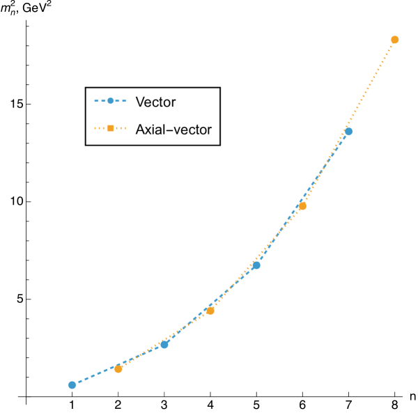
Figure 1: Meson mass spectra.

The second, dimensionless parameter of the boundary theory, $\lambda_{\text{YM}}$, can be fixed from (5.8) for $N_{c}=3$,

$$f_{\pi}=92.4\,\text{MeV}\quad\Rightarrow\quad\lambda_{\text{YM}}=\frac{54\pi^{4}f^{2}_{\pi}}{N_{c}M_{\text{KK}}^{2}}=16.69.$$ (5.11)

In some cases (references may be found in [33]) a lower value of the t’ Hooft coupling is chosen which corresponds to $f_{\pi}$ going closer to its chiral limit value of $87\,\text{MeV}$. With all the parameters of the effective theory fixed, it can be used to predict values of other interaction couplings such as $L_{1,2}$.

Beyond the quadratic order the effective action is non-local. To extract local contributions, expansion of the interaction vertices in powers of $q$ near $q\to 0$ (local expansion) is performed. In coordinate space this expansion is equivalent to gradient expansion. In the terms to be discussed in the next two Sections, the local expansion will be truncated to the leading term. An example of this procedure was demonstrated in (1.22) in the Introduction. While zero momentum limit of the projector $D^{\varkappa}_{\nu}(q)$ is actually indeterminate, the expansion procedure is well-defined.

6 Low Energy Constants

To help with identification of LECs, it should be clarified what terms in the effective action (A.5) can be matched to the LEC terms in the Chiral Lagrangian. We look for 4-derivative terms in the action. First, note that

$$B^{a}_{\mu}B^{a}_{\nu}=-4\,\text{Tr}\left(\Sigma^{-1}\partial_{\mu}\Sigma T^{a}\right)\text{Tr}\left(\Sigma^{-1}\partial_{\nu}\Sigma T^{a}\right)=-2\,\text{Tr}\left(\Sigma^{-1}\partial_{\mu}\Sigma\Sigma^{-1}\partial_{\nu}\Sigma\right)\\ =2\,\text{Tr}\left(\partial_{\mu}\Sigma^{-1}\Sigma\Sigma^{-1}\partial_{\nu}\Sigma\right)=2\,\text{Tr}\left(\partial_{\mu}\Sigma^{-1}\partial_{\nu}\Sigma\right).$$ (6.1)

With the help of this identity, the double-trace operators $L_{1,2}$ of the Chiral Lagrangian (1.1) can be rewritten in terms of $B^{a}_{\mu}$,

$$\begin{gathered}\left(\text{Tr}\left(\partial_{\mu}\Sigma^{\dagger}\partial^{\mu}\Sigma\right)\right)^{2}=\eta^{\mu\rho}\eta^{\nu\sigma}\text{Tr}\left(\partial_{\mu}\Sigma^{-1}\partial_{\rho}\Sigma\right)\text{Tr}\left(\partial_{\nu}\Sigma^{-1}\partial_{\sigma}\Sigma\right)=\frac{1}{4}\eta^{\mu\rho}\eta^{\nu\sigma}B^{a}_{\mu}B^{a}_{\rho}B^{b}_{\nu}B^{b}_{\sigma},\\[5.69046pt] \left(\text{Tr}\left(\partial_{\mu}\Sigma^{\dagger}\partial_{\nu}\Sigma\right)\right)^{2}=\eta^{\mu\rho}\eta^{\nu\sigma}\text{Tr}\left(\partial_{\mu}\Sigma^{-1}\partial_{\nu}\Sigma\right)\text{Tr}\left(\partial_{\rho}\Sigma^{-1}\partial_{\sigma}\Sigma\right)=\frac{1}{4}\eta^{\mu\rho}\eta^{\nu\sigma}B^{a}_{\mu}B^{a}_{\nu}B^{b}_{\rho}B^{b}_{\sigma}.\end{gathered}$$ (6.2)

Similarly, for the single-trace operators (1.3),

$$\begin{gathered}B^{a}_{\mu}B^{\mu,b}B^{c}_{\nu}B^{\nu,d}\,\text{Tr}\left(T^{a}T^{b}T^{c}T^{d}\right)=\text{Tr}\left(\partial_{\mu}\Sigma^{-1}\partial^{\mu}\Sigma\partial_{\nu}\Sigma^{-1}\partial^{\nu}\Sigma\right),\\[5.69046pt] B^{a}_{\mu}B^{\mu,b}B^{c}_{\nu}B^{\nu,d}\,\text{Tr}\left(T^{a}T^{c}T^{b}T^{d}\right)=\text{Tr}\left(\partial_{\mu}\Sigma^{-1}\partial_{\nu}\Sigma\partial^{\mu}\Sigma^{-1}\partial^{\nu}\Sigma\right).\end{gathered}$$ (6.3)

The equations (6.2) and (6.3) imply that in the effective action the terms with LECs must have four $B^{a}_{\mu}$ factors. Obviously, since $B_{\mu}$ contains $B^{a}_{\mu}$ (1.11), a term with four factors of $B_{\mu}$ is also a candidate for the role of a term with LECs. However, consider the following expression,

$$\partial_{\mu}B^{a}_{\nu}-\partial_{\nu}B^{a}_{\mu}=-2i\,\text{Tr}\left[\left(\partial_{\mu}\Sigma^{-1}\partial_{\nu}\Sigma-\partial_{\nu}\Sigma^{-1}\partial_{\mu}\Sigma\right)T^{a}\right].$$ (6.4)

After inserting $\mathbb{1}=\Sigma\Sigma^{-1}$ between the derivatives the above expression can be written as a commutator,

$$\partial_{\mu}B^{a}_{\nu}-\partial_{\nu}B^{a}_{\mu}=2i\,\text{Tr}\left(\left[\Sigma^{-1}\partial_{\mu}\Sigma,\Sigma^{-1}\partial_{\nu}\Sigma\right]T^{a}\right).$$ (6.5)

On the other hand, commutator of the $B$-fields (1.11) can be expressed as

$$\left[B_{\mu},B_{\nu}\right]=\left[B^{a}_{\mu}T^{a},B^{b}_{\nu}T^{b}\right]=-\left[\Sigma^{-1}\partial_{\mu}\Sigma,\Sigma^{-1}\partial_{\nu}\Sigma\right],$$ (6.6)

where the abelian parts do not contribute to the commutator. This demonstrates that the antisymmetrized derivative of $B^{a}_{\mu}$ can be rewritten as the commutator of two $B^{a}_{\mu}$,

$$2\partial_{[\mu}B^{a}_{\nu]}\equiv\partial_{\mu}B^{a}_{\nu}-\partial_{\nu}B^{a}_{\mu}=-2i\,\text{Tr}\left(\left[B_{\mu},B_{\nu}\right]T^{a}\right).$$ (6.7)

This means that some terms of the effective action may contain four $B^{a}_{\mu}$ factors only superficially: if they have an extra derivative and the indices are appropriately antisymmetrized, they are actually of higher order in $B^{a}_{\mu}$. More generally, recall that the Chiral Lagrangian is an expansion in derivatives (momenta) of $\pi$-mesons. The terms with LECs are of the order $\mathcal{O}(p^{4})$. Since $B_{\mu}$ carries within it at least one derivative of the pion, the terms with the LECs in the effective action must have the total number of $B$-fields and derivatives acting on them to be equal to four. Thus, the terms with four $B$-fields in $S_{\text{eff},15}$ and $S_{\text{eff},16}$, (A.20) and (A.21), which might potentially contribute to 4-derivative terms, are in fact of higher order in momenta and do not contribute to the values of LECs.

There are only two terms in the effective action (A.5), ($S_{\text{eff},2}$ and $S_{\text{eff},3}$), that satisfy the criteria outlined above and give rise to terms with the bare LECs of the Chiral Lagrangian. Since $B$-fields behave as derivatives under rescaling of the coordinates, any extra factors arising from converting the rescaled coordinates (2.6) into the physical ones are cancelled out by the factors from the integral measure. As such, for the remainder of this Section all discussed effective action terms will be treated as if they have already been converted into physical coordinates.

The first effective action term of interest is $S_{\text{eff},2}$ which is given by (A.7). After certain algebra (see Appendix L for details), in the local approximation $S_{\text{eff},2}$ takes the form (see (L.13))

$$\left.S_{\text{eff},2}\vphantom{\frac{1}{2}}\right|_{\text{loc}}=L^{(l)}\int d^{4}x\left[\text{Tr}\left(\partial_{\mu}\Sigma^{-1}\partial^{\mu}\Sigma\partial_{\nu}\Sigma^{-1}\partial^{\nu}\Sigma\right)-\text{Tr}\left(\partial_{\mu}\Sigma^{-1}\partial_{\nu}\Sigma\partial^{\mu}\Sigma^{-1}\partial^{\nu}\Sigma\right)\right],$$ (6.8)

where $L^{(l)}$, known since the original work [10], is

$$L^{(l)}\equiv-\kappa C=-\frac{N_{c}\lambda_{\text{YM}}}{216\pi^{3}}C.$$ (6.9)

The numerical constant $C$ is computed in (L.10),

$$C=\int\limits_{-\infty}^{+\infty}dz\,\frac{w(z)^{2}-2w(z)^{3}+w(z)^{4}}{u(z)}\approx 0.157.$$ (6.10)

The second contribution to the bare LECs comes from $S_{\text{eff},3}$. Similarly to $S_{\text{eff},2}$, taking the local approximation (details of the computation can be found in Appendix L), this contribution can be brought to the form (see (L.21))

$$\left.S_{\text{eff},3}\vphantom{\frac{1}{2}}\right|_{BJ,\text{loc}}=L^{(nl)}\int d^{4}x\left[2\text{Tr}\left(\partial_{\mu}\Sigma^{-1}\partial^{\mu}\Sigma\partial_{\nu}\Sigma^{-1}\partial^{\nu}\Sigma\right)+\text{Tr}\left(\partial_{\mu}\Sigma^{-1}\partial_{\nu}\Sigma\partial^{\mu}\Sigma^{-1}\partial^{\nu}\Sigma\right)\right],$$ (6.11)

where

$$L^{(nl)}\equiv-\frac{\kappa^{2}}{6\tilde{T}_{8}}a^{(3)}_{11}=-\frac{9N_{c}}{128\pi\lambda_{\text{YM}}}a^{(3)}_{11}.$$ (6.12)

The numerical constant $a^{(3)}_{11}$ is defined in (L.17),

$$a^{(3)}_{11}=\int\limits_{-\infty}^{+\infty}dz\,w(z)\,\partial_{z}\left(u(z)^{4}(\partial_{z}w(z))^{3}\right)=-\frac{7\Gamma\left(\frac{1}{6}\right)}{40\pi^{7/2}\Gamma\left(\frac{2}{3}\right)}\approx-0.013.$$ (6.13)

Both effective action terms, $S_{\text{eff},2}$ and $S_{\text{eff},3}$, generate the single-trace operators introduced in (1.3). Combining (6.8) and (6.11) produces the quartic $\Sigma$-field self-interaction terms

$$S^{SU(N_{f})}_{\text{quart}}\equiv\int d^{4}x\left[L^{SU(N_{f})}_{3}\,\text{Tr}\left(\partial_{\mu}\Sigma^{-1}\partial^{\mu}\Sigma\partial_{\nu}\Sigma^{-1}\partial^{\nu}\Sigma\right)\right.\\ \left.+\tilde{L}^{SU(N_{f})}_{3}\,\text{Tr}\left(\partial_{\mu}\Sigma^{-1}\partial_{\nu}\Sigma\partial^{\mu}\Sigma^{-1}\partial^{\nu}\Sigma\right)\right],$$ (6.14)

where

$$L^{SU(N_{f})}_{3}\equiv 2L^{(nl)}+L^{(l)},\qquad\tilde{L}^{SU(N_{f})}_{3}\equiv L^{(nl)}-L^{(l)},$$ (6.15)

are the bare LECs for arbitrary $N_{f}$. We notice that, contrary to expectations, no independent double-trace operators labeled by $L_{1,2}$ emerge here. For $N_{f}=2$, they will appear through relations between the single- and double-trace operators (see below).

$\bullet$ Pion elastic scattering

Consider now the quartic action (6.14) expanded to the leading order in the $\pi$-fields

$$\left.S^{SU(N_{f})}_{\text{quart}}\vphantom{\frac{1}{2}}\right|_{\mathcal{O}\left(\pi^{4}\right)}=\frac{16}{f^{4}_{\pi}}\int d^{4}x\left(L^{SU(N_{f})}_{3}\partial_{\mu}\pi^{a}\partial^{\mu}\pi^{b}\partial_{\nu}\pi^{c}\partial^{\nu}\pi^{d}\right.\\ \left.+\tilde{L}^{SU(N_{f})}_{3}\partial_{\mu}\pi^{a}\partial_{\nu}\pi^{b}\partial^{\mu}\pi^{c}\partial^{\nu}\pi^{d}\right)\text{Tr}\left(T^{a}T^{b}T^{c}T^{d}\right).$$ (6.16)

For arbitrary $N_{f}$ the trace of four generators is given by (N.6), which simplifies the expression

$$\left.S^{SU(N_{f})}_{\text{quart}}\vphantom{\frac{1}{2}}\right|_{\mathcal{O}\left(\pi^{4}\right)}=\frac{4L^{SU(N_{f})}_{3}}{f^{4}_{\pi}}\int d^{4}x\,\partial_{\mu}\pi^{a}\partial^{\mu}\pi^{b}\partial_{\nu}\pi^{c}\partial^{\nu}\pi^{d}\left(\frac{1}{N_{f}}\delta_{ab}\delta_{cd}+\frac{1}{2}d_{abe}d_{cde}\right)\\ +\frac{4\tilde{L}^{SU(N_{f})}_{3}}{f^{4}_{\pi}}\int d^{4}x\,\partial_{\mu}\pi^{a}\partial_{\nu}\pi^{b}\partial^{\mu}\pi^{c}\partial^{\nu}\pi^{d}\\ \times\left[\frac{1}{N_{f}}\left(2\delta_{ab}\delta_{cd}-\delta_{ac}\delta_{bd}\right)+\frac{1}{2}\left(2d_{abe}d_{cde}-d_{ace}d_{bde}\right)\right].$$ (6.17)

This action term is responsible for $2\rightarrow 2$ elastic pion scattering,

$$\pi^{a}(p_{a})+\pi^{b}(p_{b})\to\pi^{c}(p_{c})+\pi^{d}(p_{d}).$$ (6.18)

The $T$-matrix element for this process:

$$S=I+iT,\qquad T=(2\pi)^{4}\delta\left(p_{a}+p_{b}-p_{c}-p_{d}\right)M.$$ (6.19)

The tree-level scattering amplitude $M$ (or rather its low energy limit) can be straightforwardly read off from (6.17),

$$M^{SU(N_{f})}=\delta_{ab}\delta_{cd}A^{SU(N_{f})}(s,t,u)+\delta_{ac}\delta_{bd}A^{SU(N_{f})}(t,s,u)+\delta_{ad}\delta_{bc}A^{SU(N_{f})}(u,t,s)\\ +\frac{N_{f}}{2}\left(A^{SU(N_{f})}(s,t,u)d_{abe}d_{cde}+A^{SU(N_{f})}(t,s,u)d_{ace}d_{bde}+A^{SU(N_{f})}(u,t,s)d_{ade}d_{bce}\right),$$ (6.20a)

$$A^{SU(N_{f})}(s,t,u)\equiv\frac{8\left(L^{SU(N_{f})}_{3}-\tilde{L}^{SU(N_{f})}_{3}\right)}{N_{f}f^{4}_{\pi}}s^{2}+\frac{8\tilde{L}^{SU(N_{f})}_{3}}{N_{f}f^{4}_{\pi}}\left(t^{2}+u^{2}\right),$$ (6.20b)

where the Mandelstam variables are defined as

$$s=-\left(p_{a}+p_{b}\right)^{2},\qquad t=-\left(p_{a}-p_{c}\right)^{2},\qquad u=-\left(p_{a}-p_{d}\right)^{2}.$$ (6.21)

Note the appearance of the terms proportional to the product of $d$-tensors in the amplitude (6.20a).

$\bullet$ $\bm{N_{f}=3}$

Let us now project the above results on $N_{f}=3$. In this case the $\tilde{L}_{3}$ operator (1.3) is not independent. With the help of the Cayley-Hamilton relation [14],

$$\text{Tr}\left(ABAB\right)=-2\,\text{Tr}\left(A^{2}B^{2}\right)+\frac{1}{2}\,\text{Tr}\left(A^{2}\right)\text{Tr}\left(B^{2}\right)+\left(\text{Tr}\left(AB\right)\right)^{2},\qquad A,B\in\mathfrak{su}(3),$$ (6.22)

the $\tilde{L_{3}}$ operator can be rewritten as a linear combination of $L_{1}$, $L_{2}$, and $L_{3}$ operators. Specifically,

$$\text{Tr}\left(\partial_{\mu}\Sigma^{-1}\partial_{\nu}\Sigma\partial^{\mu}\Sigma^{-1}\partial^{\nu}\Sigma\right)=\text{Tr}\left(\Sigma^{-1}\partial_{\mu}\Sigma\Sigma^{-1}\partial_{\nu}\Sigma\Sigma^{-1}\partial^{\mu}\Sigma\Sigma^{-1}\partial^{\nu}\Sigma\right)\\ =-2\,\text{Tr}\left(\partial_{\mu}\Sigma^{-1}\partial^{\mu}\Sigma\partial_{\nu}\Sigma^{-1}\partial^{\nu}\Sigma\right)+\frac{1}{2}\left(\text{Tr}\left(\partial_{\mu}\Sigma^{-1}\partial^{\mu}\Sigma\right)\right)^{2}+\left(\text{Tr}\left(\partial_{\mu}\Sigma^{-1}\partial_{\nu}\Sigma\right)\right)^{2}.$$ (6.23)

Substituting (6.23) into the quartic action (6.14) for the $\Sigma$-field gives

$$S^{SU(3)}_{\text{quart}}=\int d^{4}x\left[L^{SU(3)}_{1}\left(\text{Tr}\left(\partial_{\mu}\Sigma^{-1}\partial^{\mu}\Sigma\right)\right)^{2}+L^{SU(3)}_{2}\left(\text{Tr}\left(\partial_{\mu}\Sigma^{-1}\partial_{\nu}\Sigma\right)\right)^{2}\right.\\ \left.+L^{SU(3)}_{3}\text{Tr}\left(\partial_{\mu}\Sigma^{-1}\partial^{\mu}\Sigma\partial_{\nu}\Sigma^{-1}\partial^{\nu}\Sigma\right)\right],$$ (6.24)

where $SU(3)$ bare LECs are defined as

$$L^{SU(3)}_{2}=2L^{SU(3)}_{1}=\tilde{L}^{SU(N_{f})}_{3}=L^{(nl)}-L^{(l)},\qquad L^{SU(3)}_{3}=L^{SU(N_{f})}_{3}-2\tilde{L}^{SU(N_{f})}_{3}=3L^{(l)}.$$ (6.25)

Here, the definitions (6.15) were used in the last step. The amplitude of the pion elastic scattering can be computed directly from (6.24) with the result,

$$M^{SU(3)}=\delta_{ab}\delta_{cd}A^{SU(3)}(s,t,u)+\delta_{ac}\delta_{bd}A^{SU(3)}(t,s,u)+\delta_{ad}\delta_{bc}A^{SU(3)}(u,t,s)\\ +\frac{4L^{SU(3)}_{3}}{f^{4}_{\pi}}\left(s^{2}d_{abe}d_{cde}+t^{2}d_{ace}d_{bde}+u^{2}d_{ade}d_{bce}\right),$$ (6.26a)

$$A^{SU(3)}(s,t,u)\equiv\frac{8L^{SU(3)}_{1}}{f^{4}_{\pi}}s^{2}+\frac{8L^{SU(3)}_{3}}{3f^{4}_{\pi}}s^{2}+\frac{4L^{SU(3)}_{2}}{f^{4}_{\pi}}\left(t^{2}+u^{2}\right).$$ (6.26b)

The amplitude (6.26) depends on two coefficients only — it is either expressible in terms of $L^{(l)}$ and $L^{(nl)}$ or $L^{SU(N_{f})}_{3}$ and $\tilde{L}^{SU(N_{f})}_{3}$. The amplitude (6.26) can be obtained directly from (6.20) substituting $N_{f}=3$ and utilizing the relation (N.10) for the $d$-tensors.

$\bullet$ $\bm{N_{f}=2}$

Finally, we separately consider the $N_{f}=2$ case. Fro $N_{f}=2$, both single-trace operators (1.3) are expressible in terms of the double trace operators $L_{1,2}$. In addition to (6.23), which is also valid for $N_{f}=2$, we use [14],

$$2\,\text{Tr}\left(ABCD\right)=\text{Tr}\left(AB\right)\text{Tr}\left(CD\right)-\text{Tr}\left(AC\right)\text{Tr}\left(BD\right)+\text{Tr}\left(AD\right)\text{Tr}\left(BC\right)$$ (6.27)

for $A,B,C,D\in\mathfrak{su}(2)$. Specifically,

$$\text{Tr}\left(\partial_{\mu}\Sigma^{-1}\partial^{\mu}\Sigma\partial_{\nu}\Sigma^{-1}\partial^{\nu}\Sigma\right)=\text{Tr}\left(\Sigma^{-1}\partial_{\mu}\Sigma\Sigma^{-1}\partial^{\mu}\Sigma\Sigma^{-1}\partial_{\nu}\Sigma\Sigma^{-1}\partial^{\nu}\Sigma\right)\\ =\frac{1}{2}\left(\text{Tr}\left(\Sigma^{-1}\partial_{\mu}\Sigma\Sigma^{-1}\partial^{\mu}\Sigma\right)\right)^{2}=\frac{1}{2}\left(\text{Tr}\left(\partial_{\mu}\Sigma^{-1}\partial^{\mu}\Sigma\right)\right)^{2}.$$ (6.28)

The last two terms on the right-hand side of (6.27) cancelled each other out and the $L_{3}$ operator is completely expressible in terms of the $L_{1}$ operator. Substituting (6.23) and (6.28) into (6.14), the quartic action term for the $\Sigma$-field reads

$$S^{SU(2)}_{\text{quart}}=\int d^{4}x\left[L^{SU(2)}_{2}\left(\text{Tr}\left(\partial_{\mu}\Sigma^{-1}\partial^{\mu}\Sigma\right)\right)^{2}+L^{SU(2)}_{2}\left(\text{Tr}\left(\partial_{\mu}\Sigma^{-1}\partial_{\nu}\Sigma\right)\right)^{2}\right],$$ (6.29)

where the $SU(2)$ bare LECs are defined as

$$\begin{gathered}L^{SU(2)}_{1}=L^{SU(3)}_{1}+\frac{L^{SU(3)}_{3}}{2}=\frac{L^{SU(N_{f})}_{3}-\tilde{L}^{SU(N_{f})}_{3}}{2}=\frac{L^{(nl)}}{2}+L^{(l)},\\[5.69046pt] L^{SU(2)}_{2}=L^{SU(3)}_{2}=\tilde{L}^{SU(N_{f})}_{3}=L^{(nl)}-L^{(l)}.\end{gathered}$$ (6.30)

Here, the relations (6.15) and (6.25) were used to connect $SU(2)$ couplings to the bare LECs for $N_{f}=3$ and arbitrary $N_{f}$. The elastic pion scattering tree level amplitude is again easily computed based on the quartic action (6.29). The result is well-known in the literature it is given by [13, 38, 53, 54, 55, 56],

$$M=\delta_{ab}\delta_{cd}A(s,t,u)+\delta_{ac}\delta_{bd}A(t,s,u)+\delta_{ad}\delta_{bc}A(u,t,s),$$ (6.31a)

$$A(s,t,u)=\frac{s}{f^{2}_{\pi}}+\frac{8\mathbb{L}^{SU(2)}_{1}}{f^{4}_{\pi}}s^{2}+\frac{4\mathbb{L}^{SU(2)}_{2}}{f^{4}_{\pi}}(t^{2}+u^{2}),$$ (6.31b)

where the linear in $s$ contribution in $A(s,t,u)$ comes from the $\Sigma\Sigma$ term of the free action (5.7) and is unrelated to the quartic in $\Sigma$ terms discussed in this Section (we have omitted this term in (6.20b)). In (6.31b), the effective LECs are defined as

$$\mathbb{L}^{SU(2)}_{1}\equiv L^{SU(2)}_{1}=\frac{L^{(nl)}}{2}+L^{(l)},\qquad\mathbb{L}^{SU(2)}_{2}\equiv L^{SU(2)}_{2}=L^{(nl)}-L^{(l)}.$$ (6.32)

The very same result for the amplitude can be obtained directly from (6.20) substituting $N_{f}=2$ and recalling that the $d$-tensors vanish in $SU(2)$.

The coefficient $L^{{(nl)}}$, which stems from the higher order expansion of the DBI action was first introduced and discussed in [38]. Evidently, $L^{(l)}$ and $L^{{(nl)}}$ have different parametric dependence,

$$L^{(l)}=\mathcal{O}\left(N_{c}\lambda_{\text{YM}}\right),\qquad L^{(nl)}=\mathcal{O}\left(\frac{N_{c}}{\lambda_{\text{YM}}}\right).$$ (6.33)

Since the ’t Hooft constant was fixed in (5.11) to a finite value greater than 1, $L^{(nl)}$ is suppressed compared to $L^{(l)}$.

For $N_{f}=2$ our results are in full agreement with [38]. For $N_{f}\geq 3$, we find the discussion in [38] somewhat confusing since it makes no sharp distinction between the bare and effective LECs. The point, which we hopefully have clarified here, is that the two sets of LECs are not equivalent. While the effective LECs are physical and measurable, the bare ones could be altered by vector meson field redefinitions. We demonstrate this point explicitly in Appendix M on the example of the original works [10, 11].

$\bullet$ Vector meson exchange contributions to the amplitude.

The pion scattering amplitude can also acquire contributions from the tree level vector meson exchange. The effective action (A.5) does contain terms that could potentially generate such contributions. One candidate is $S_{\text{eff},6}$ (A.11) in the local approximation (except for the integral in the third line),

$$\left.S_{\text{eff},6}\vphantom{\frac{1}{2}}\right|_{\text{loc}}=\sum_{n}\frac{if_{abc}\kappa a^{(2)}_{6,n}}{2(2\pi)^{2}}\int d^{4}q\,d^{4}p\left(2\eta^{\mu\rho}\eta^{\nu\sigma}-\eta^{\mu\sigma}\eta^{\nu\rho}-\eta^{\mu\nu}\eta^{\rho\sigma}\right)p_{\rho}B^{a}_{\nu}(-q)\,B^{b}_{\sigma}(p)\,V^{c}_{\mu,n}(q-p)\\ -\sum_{n}\frac{if_{abc}\kappa a^{(2)}_{6,n}}{2(2\pi)^{2}}\int d^{4}q\,d^{4}p\left(2\eta^{\mu\nu}\eta^{\rho\sigma}-\eta^{\mu\sigma}\eta^{\nu\rho}\right)p_{\rho}B^{a}_{\nu}(-q)\,B^{b}_{\sigma}(q-p)\,V^{c}_{\mu,n}(p)\\ -\sum_{n}\frac{if_{abc}\kappa}{2(2\pi)^{2}}\int d^{4}q\,d^{4}p\left(a^{(2)}_{6,n}+\kappa\int dz\left(q^{2}-\lambda_{n}\right)\frac{\psi_{n}(z)}{u(z)}\,\hat{s}^{(2)}_{5}(q,z)\right)\\ \times\left(2\eta^{\mu\rho}\eta^{\nu\sigma}-\eta^{\mu\sigma}\eta^{\nu\rho}-\eta^{\mu\nu}\eta^{\rho\sigma}\right)p_{\rho}B^{a}_{\sigma}(p)\,B^{b}_{\mu}(q-p)\,V^{c}_{\nu,n}(-q)\\ -\sum_{n}\frac{if_{abc}\kappa}{(2\pi)^{2}}\frac{\mathcal{C}_{n}}{\lambda_{n}}\int d^{4}q\,d^{4}p\,\left(\eta^{\mu\rho}\eta^{\nu\sigma}-\eta^{\mu\nu}\eta^{\rho\sigma}\right)p_{\rho}B^{a}_{\sigma}(p)\,B^{b}_{\mu}(q-p)\,V^{c}_{\nu,n}(-q).$$ (6.34)

Each integral in (6.34) contains at least three derivatives (one from $p_{\rho}$ and two more from the $B$-fields). Therefore, the resulting contribution to the amplitude (6.31b) is of the order $\mathcal{O}\left(p^{6}\right)$, while the effective LECs emerge at the order $\mathcal{O}\left(p^{4}\right)$. Consequently, the effective action term (6.34) does not affect the values of the effective LECs.

Similarly, consider $S_{\text{eff,5}}$ (A.10), which, after taking the local approximation, takes the form (in the coordinate space)

$$\left.S_{\text{eff},5}\vphantom{\frac{1}{2}}\right|_{\text{loc}}=-\sum_{n}\frac{N_{c}\varepsilon^{z\mu\nu\rho\sigma}a^{(2)}_{1,n}}{8\pi^{2}}\int d^{4}x\,\text{STr}\left[B_{\nu}B_{\rho}\partial_{\mu}V_{\sigma,n}\right],$$ (6.35)

where the relation (A.2) was used. The $\pi\pi V$ vertex read off from (6.35) is $\mathcal{O}\left(p^{3}\right)$ thus contributing $\mathcal{O}\left(p^{6}\right)$ to the amplitude. In fact, the contribution of $S_{\text{eff,5}}$ is even further suppressed: the symmetrized trace in (6.35) is symmetric over $\nu\leftrightarrow\rho$, when contracted with the antisymmetric Levi-Civita tensor it renders the entire integral to vanish.

In summary, while tree level exchanges of the vector mesons could potentially contribute to the effective LECs, they do not. Basically, the vector mesons are irrelevant at this order in momenta and could be thought as being partially integrated out.

7 Vector Meson Interactions in the Effective Action

$\bullet$ CS-induced.

As an example of interactions between the vector mesons $V_{\mu,n}$ and the $B$-field (which contains the pions and $\eta^{\prime}$-meson), we focus on $S_{\text{eff},7}$ (A.12). This term is induced by the CS action. Its distinguishing property (compared to the DBI-induced terms) is the presence of the Levi-Civita pseudotensor. Applying the truncated local expansion (which makes it possible to write the expression in coordinate space),

$$\left.S_{\text{eff},7}\vphantom{\frac{1}{2}}\right|_{\text{loc}}=-\sum_{n,m}\frac{N_{c}\varepsilon^{z\mu\nu\rho\sigma}a^{(2)}_{2,nm}}{4\pi^{2}}\int d^{4}x\,\text{STr}\left(B_{\nu}\partial_{\mu}V_{\rho,n}V_{\sigma,m}\right).$$ (7.1)

The relation (A.2) was used here. The coupling is given by the integral

$$a^{(2)}_{2,nm}=\int\limits_{-\infty}^{+\infty}dz\,w(z)\,\psi_{n}(z)\,\partial_{z}\psi_{m}(z).$$ (7.2)

Appendix G contains a set of values for this constant obtained numerically. Substituting the leading order expansion (1.13) of the $B$-field into (7.1) gives the following interaction terms

$$\left.S_{\text{eff},7}\vphantom{\frac{1}{2}}\right|_{\text{loc},\mathcal{O}\left(\pi,\eta\right)}=\sum_{n,m}\frac{N_{c}\varepsilon^{z\mu\nu\rho\sigma}a^{(2)}_{2,nm}}{4\pi^{2}f_{\pi}}\sqrt{\frac{2}{N_{f}}}\int d^{4}x\,\partial_{\nu}\eta^{\prime}\,\text{STr}\left(\partial_{\mu}V_{\rho,n}V_{\sigma,m}\right)\\ +\sum_{n,m}\frac{N_{c}\varepsilon^{z\mu\nu\rho\sigma}a^{(2)}_{2,nm}}{2\pi^{2}f_{\pi}}\int d^{4}x\,\partial_{\nu}\pi^{a}\,\text{STr}\left(\partial_{\mu}V_{\rho,n}V_{\sigma,m}T^{a}\right).$$ (7.3)

These two terms represent (derivative) interactions of the $\pi$ and $\eta^{\prime}$ mesons with the vector meson multiplets. For example, taking $n=m=1$ in the second term, which corresponds to the lightest vector mesons, produces an interaction resembling the $\omega\to\rho\pi$ process, which is known experimentally.

Superficially, it seems that the CS-induced interaction terms (7.3) might be parity-violating due to the presence of the Levi-Civita pseudotensor. This is not the case, however. The terms in (7.3) contain even number of derivatives. The sign change from the Levi-Civita pseudotensor under the spatial parity transformation is compensated by the extra minus sign from the pseudoscalar fields $\eta^{\prime}$ or $\pi^{a}$. Since the vector mesons enter quadratically, the entire term conserves parity if both vector mesons are of the same parity.

Let us now consider the case when the vector mesons have opposite parities. Integrating the coefficient $a^{(2)}_{2,nm}$ by parts gives:

$$a^{(2)}_{2,nm}=\int\limits_{-\infty}^{+\infty}dz\,w(z)\,\psi_{n}(z)\,\partial_{z}\psi_{m}(z)=\left.w(z)\,\psi_{n}(z)\,\psi_{m}(z)\right|_{z\to\pm\infty}\\ -\frac{1}{\pi}\int\limits_{-\infty}^{+\infty}dz\,\frac{\psi_{n}(z)\,\psi_{m}(z)}{u(z)^{3}}-\int\limits_{-\infty}^{+\infty}dz\,w(z)\,\partial_{z}\psi_{n}(z)\,\psi_{m}(z).$$ (7.4)

The boundary term is zero due to asymptotics (F.4) of eigenfunctions. Since the eigenfunctions also have opposite parities, the second, integral term is also zero since it is an integral of an odd function over a symmetric interval. The last integral can be identified as $a^{(2)}_{2,mn}$. Thus, for mesons of opposite parities:

$$a^{(2)}_{2,nm}=-a^{(2)}_{2,mn},\qquad n,m\text{ --- opposite parity}.$$ (7.5)

Integrating the second line in the effective action term (7.3) by parts gives (the same can be done for the first line as well)

$$\left.S_{\text{eff},7}\vphantom{\frac{1}{2}}\right|_{\begin{subarray}{c}\text{loc},\\ \mathcal{O}\left(\pi\right)\end{subarray}}=-\sum_{n,m}\frac{N_{c}\varepsilon^{z\mu\nu\rho\sigma}a^{(2)}_{2,nm}}{2\pi^{2}f_{\pi}}\int d^{4}x\,\text{STr}\left(\partial_{\mu}\partial_{\nu}\pi^{a}V_{\rho,n}V_{\sigma,m}T^{a}+\partial_{\nu}\pi^{a}V_{\rho,n}\partial_{\mu}V_{\sigma,m}T^{a}\right).$$ (7.6)

The first term under the symmetrized trace is symmetric over $\mu\leftrightarrow\nu$ and it is contracted with the antisymmetric Levi-Civita pseudotensor, thus, it is zero. After renaming $\rho\leftrightarrow\sigma$ and $n\leftrightarrow m$ in the second term, utilizing the relation (7.5), and reordering factors under the symmetrized trace,

$$\left.S_{\text{eff},7}\vphantom{\frac{1}{2}}\right|_{\begin{subarray}{c}\text{loc},\mathcal{O}\left(\pi\right),\\ n,m\text{ --- opp. par.}\end{subarray}}=-\sum_{n,m}\frac{N_{c}\varepsilon^{z\mu\nu\rho\sigma}a^{(2)}_{2,nm}}{2\pi^{2}f_{\pi}}\int d^{4}x\,\partial_{\nu}\pi^{a}\,\text{STr}\left(\partial_{\mu}V_{\rho,n}V_{\sigma,m}T^{a}\right),$$ (7.7)

which is the original effective action term (second line of (7.3)), but with the opposite sign. This means that this integral must be equal to zero. As such, there are no CS-induced parity-violating interactions, as expected.

$\bullet$ DBI-induced.

Consider $S_{\text{eff},8}$ (A.13) which is induced by the DBI action. The leading term of the local expansion can be written in coordinate space (converting the coefficients with (A.2)),

$$\left.S_{\text{eff},8}\vphantom{\frac{1}{2}}\right|_{\text{loc}}=\sum_{n,m}f_{abc}\kappa a^{(2)}_{7,nm}\int d^{4}x\left(2\eta^{\mu\rho}\eta^{\nu\sigma}-\eta^{\mu\sigma}\eta^{\nu\rho}\right)B^{a}_{\nu}V^{b}_{\mu,n}\partial_{\rho}V^{c}_{\sigma,m},$$ (7.8)

where

$$a^{(2)}_{7,nm}\equiv\int\limits_{-\infty}^{+\infty}dz\,w(z)\,\frac{\psi_{n}(z)\,\psi_{m}(z)}{u(z)}.$$ (7.9)

The results of the numerical analysis for this coupling for a few lowest $n$ and $m$ can be found in Appendix G. Replacing the structure constants with (N.3) gives

$$\left.S_{\text{eff},8}\vphantom{\frac{1}{2}}\right|_{\text{loc}}=-\sum_{n,m}2i\kappa a^{(2)}_{7,nm}\int d^{4}x\left(2\eta^{\mu\rho}\eta^{\nu\sigma}-\eta^{\mu\sigma}\eta^{\nu\rho}\right)B^{a}_{\nu}\,\text{Tr}\left(\left[V_{\mu,n},\partial_{\rho}V_{\sigma,m}\right]T^{a}\right).$$ (7.10)

After substituting the leading term of the expansion (1.13) of $B^{a}_{\nu}$,

$$\left.S_{\text{eff},8}\vphantom{\frac{1}{2}}\right|_{\text{loc},\mathcal{O}\left(\pi\right)}=\sum_{n,m}\frac{4i\kappa a^{(2)}_{7,nm}}{f_{\pi}}\int d^{4}x\left(2\eta^{\mu\sigma}\eta^{\nu\rho}-\eta^{\mu\nu}\eta^{\rho\sigma}\right)\partial_{\nu}\pi^{a}\,\text{Tr}\left(\left[\partial_{\mu}V_{\rho,n},V_{\sigma,m}\right]T^{a}\right),$$ (7.11)

where some indices were renamed to facilitate comparison with (7.3). This interaction term can encode processes such as $\rho(1450)\to\left(a_{1}(1260)+\pi\right)_{P\text{-wave}}$, which was seen experimentally [51].

The DBI-induced interaction (7.11) with vector mesons of the same parities does not respect the spatial parity symmetry. However, all such terms are, in fact, zero. Consider the following integral, which is zero, if the eigenfunctions have the same parity,

$$\int\limits_{-\infty}^{+\infty}dz\left(2w(z)-1\right)g^{(2)}_{7,nm}(z)=\int\limits_{-\infty}^{+\infty}dz\left(2w(z)-1\right)\frac{\psi_{n}(z)\,\psi_{m}(z)}{u(z)}=0,$$ (7.12)

since $2w(z)-1\propto\arctan z$ is an odd function, the fraction is an even function and the integration is over a symmetric interval. The left-hand side can be written as

$$\int\limits_{-\infty}^{+\infty}dz\left(2w(z)-1\right)g^{(2)}_{7,nm}(z)=2a^{(2)}_{7,nm}-\int\limits_{-\infty}^{+\infty}dz\,g^{(2)}_{7,nm}(z),$$ (7.13)

which means that

$$a^{(2)}_{7,nm}=\frac{1}{2}\int\limits_{-\infty}^{+\infty}dz\,\frac{\psi_{n}(z)\,\psi_{m}(z)}{u(z)}=\frac{\delta_{nm}}{2\kappa},\qquad n,m\text{ --- same parity},$$ (7.14)

where we used the defintion (A.1) of the $a$-coefficients and the orthonormality (F.5) of the eigenfunctions. The contribution of the same parity vector mesons in (7.11) can be written as

$$\left.S_{\text{eff},8}\vphantom{\frac{1}{2}}\right|_{\begin{subarray}{c}\text{loc},\mathcal{O}\left(\pi\right),\\ n,m\text{ --- same par.}\end{subarray}}=\sum_{n}\frac{2i}{f_{\pi}}\int d^{4}x\left(2\eta^{\mu\sigma}\eta^{\nu\rho}-\eta^{\mu\nu}\eta^{\rho\sigma}\right)\partial_{\nu}\pi^{a}\,\text{Tr}\left(\left[\partial_{\mu}V_{\rho,n},V_{\sigma,n}\right]T^{a}\right).$$ (7.15)

The integral in (7.15) can be integrated by parts,

$$\int d^{4}x\left(2\eta^{\mu\sigma}\eta^{\nu\rho}-\eta^{\mu\nu}\eta^{\rho\sigma}\right)\partial_{\nu}\pi^{a}\,\text{Tr}\left(\left[\partial_{\mu}V_{\rho,n},V_{\sigma,n}\right]T^{a}\right)\\ =-\int d^{4}x\left(2\eta^{\mu\sigma}\eta^{\nu\rho}-\eta^{\mu\nu}\eta^{\rho\sigma}\right)\pi^{a}\,\text{Tr}\left(\left[\partial_{\mu}\partial_{\nu}V_{\rho,n},V_{\sigma,n}\right]T^{a}\right)\\ -\int d^{4}x\left(2\eta^{\mu\sigma}\eta^{\nu\rho}-\eta^{\mu\nu}\eta^{\rho\sigma}\right)\pi^{a}\,\text{Tr}\left(\left[\partial_{\mu}V_{\rho,n},\partial_{\nu}V_{\sigma,n}\right]T^{a}\right).$$ (7.16)

In the second integral if the indices $\mu\leftrightarrow\nu$ and $\rho\leftrightarrow\sigma$ are simultaneously swapped, the same integral is obtained, but with an opposite sign. Thus, the entire integral is equal to zero. In the first integral the first term in the brackets, $2\eta^{\mu\sigma}\eta^{\nu\rho}$, can be dropped because of the transversality (4.28) of the mesons. For the last remaining term we explicitly write down the sums over the Lorentz indices (recall, that the signature is mostly minus),

$$\int d^{4}x\,\eta^{\mu\nu}\eta^{\rho\sigma}\pi^{a}\,\text{Tr}\left(\left[\partial_{\mu}\partial_{\nu}V_{\rho,n},V_{\sigma,n}\right]T^{a}\right)=\int d^{4}x\,\pi^{a}\,\text{Tr}\left(\left[\partial_{0}\partial_{0}V_{0,n},V_{0,n}\right]T^{a}\right)\\ -\int d^{4}x\,\pi^{a}\,\text{Tr}\left(\left[\partial_{0}\partial_{0}V_{i,n},V_{i,n}\right]T^{a}\right)-\int d^{4}x\,\pi^{a}\,\text{Tr}\left(\left[\partial_{i}\partial_{i}V_{0,n},V_{0,n}\right]T^{a}\right)\\ +\int d^{4}x\,\pi^{a}\,\text{Tr}\left(\left[\partial_{i}\partial_{i}V_{j,n},V_{j,n}\right]T^{a}\right).$$ (7.17)

Changing the integration variable $x^{i}\to-x^{i}$ does not change integration measure (minus signs from $d^{3}x$ compensate changes in the direction of integration). Since the integrands in each of the integrals are quadratic in the vector meson components and derivatives, the behavior of the integrand under $x^{i}\to-x^{i}$ is determined solely by the properties of $\pi$-meson which is pseudoscalar. As such, every integral attains an extra minus sign from such variable change, which means that

$$\int d^{4}x\,\eta^{\mu\nu}\eta^{\rho\sigma}\pi^{a}\,\text{Tr}\left(\left[\partial_{\mu}\partial_{\nu}V_{\rho,n},V_{\sigma,n}\right]T^{a}\right)=0.$$ (7.18)

Thus, we conclude that all the DBI-induced parity-violating terms vanish as expected.

The difference between the CS-induced and DBI-induced interactions terms is clear: the former only encodes the interactions involving the vector mesons of the same parities, while the latter describes reactions of vector mesons of opposite parities. Furthermore, there is no interaction between $\eta^{\prime}$ and the vector mesons in the DBI induced interaction term (7.11). In the $\pi$-sector this term is relatively suppressed by the t’ Hooft coupling compared to (7.3),

$$\frac{\left.S_{\text{eff},7}\vphantom{\frac{1}{2}}\right|_{\text{loc},\mathcal{O}\left(\pi\right)}}{\left.S_{\text{eff},8}\vphantom{\frac{1}{2}}\right|_{\text{loc},\mathcal{O}\left(\pi\right)}}=\mathcal{O}\left(\frac{N_{c}}{\kappa}\right)=\mathcal{O}\left(\frac{1}{\lambda_{\text{YM}}}\right).$$ (7.19)

$\bullet$ A comment on the Wess-Zumino term.

The Wess-Zumino(-Witten) (WZ) term [57, 58] was originally introduced to implement the chiral anomaly [14] within chiral perturbation theory. The expression for the WZ term is written in terms of $\Sigma$ and the left/right external gauge fields $l_{\mu}$ and $r_{\mu}$. In the SS model, the WZ term is derivable from the CS action [10] upon introduction of the external gauge fields as additional sources at the boundary.

In the present work we opted not to include these external gauge fields. As such, the CS-induced terms in the obtained effective action cannot be directly identified with the WZ term. Yet, some of the terms do resemble the WZ term. For instance, consider the following contribution to the WZ term (quoted from [14] up to normalization and some notational adjustments),

$$S_{\text{WZ}}\propto\varepsilon^{\mu\nu\alpha\beta}\int d^{4}x\left[\text{Tr}\left(\Sigma^{-1}\partial_{\mu}\Sigma l_{\nu}\partial_{\alpha}l_{\beta}\right)+\text{Tr}\left(\Sigma^{-1}\partial_{\mu}\Sigma\partial_{\nu}l_{\alpha}l_{\beta}\right)\right],$$ (7.20)

The expression (7.20) resembles (7.1) from the effective action if the left gauge fields are replaced by the vector mesons.

8 Concluding Discussions

In this work we have derived the effective action for light pseudoscalar and heavy vector mesons stemming from the SS model in the holographic off-shell formalism. The DBI action of the SS model was expanded up to fourth order in the bulk field strength. The degrees of freedom of the effective action are the multiplets of massless pions, $\eta^{\prime}$-meson, and towers of heavy (axial-)vector meson multiplets. The latter can be thought of as being integrated into the action. The resulting action (see (A.5) in Appendix A) is non-linear, non-local, and rich in physical phenomena.

For arbitrary $N_{f}$, we determined the values of bare and effective LECs as well as the amplitudes of elastic pion scattering induced by the effective action. For $N_{f}=2$ our results are in complete agreement with [38]. For larger $N_{f}$ we clarify the difference between the bare and effective LECs. The obtained scattering amplitude, particularly for $SU(3)$, is of phenomenological relevance as it can be used to analyze decays of kaons into pions.

We also discussed the interactions between the pseudoscalar and vector meson sectors that can be extracted from the obtained effective action. This direction is particularly interesting in light of the recent work on the radiative vector meson decays [33]. The CS and DBI actions are responsible for different types of interactions. We observed that the CS-induced terms describe interactions involving vector mesons with identical parities while the DBI-induced terms pertain to mesons with opposite parities. At the same time, the DBI-induced interactions are parametrically suppressed compared to the CS-induced ones.

The SS model possesses a natural energy scale, $M_{\text{KK}}$, which corresponds to the energy cutoff of the effective theory on the boundary. As such the degrees of freedom of the effective theory should have energies not exceeding this scale. Indeed, if the off-shell vector mesons $V_{\mu,n}$ were not introduced in Section 4, the only remaining degrees of freedom would be $\pi$- and $\eta^{\prime}$-mesons. When vector mesons are integrated in, the cutoff moves up and may constitute the extension of the energy region of the effective theory. If a finite tower of the vector mesons is introduced, this can be viewed as extending the region of the theory’s applicability up to the mass of the heaviest meson.

The inclusion of all orders in the gradient expansion, which manifests in the non-locality of the effective action, makes the effective theory relativistically causal. Since the tower of heavy vector mesons is infinite (and thus effective energy region may be also thought to be infinite), there is space to speculate that the resulting effective action might be UV complete. Quite obviously, vector meson loops generated by the terms such as (A.17) and (A.19) (schematically, $B^{2}V^{2}$ and $V^{4}$) would produce UV divergences. There exists a hypothetical scenario that the divergencies might eventually cancel due to summation over the vector meson towers. This is hard to check, however, since such a check would require knowledge of the entire meson spectra and couplings. These couplings are given by integrals involving the eigenfunctions $\psi_{n}$, which are not known at the moment. Thus exploring this spectral problem might be worth pursuing. Applying the spectral parameter power series method [59] looks like a promising direction for the future.
 
Acknowledgements. We thank Sergey Afonin, Yanyan Bu, Maxim Nefedov, Jacob Sonnenschein, and Ismail Zahed for useful and illuminating discussions. This research was funded by Binational Science Foundation grants #2021789 and #2022132, by the ISF grant #910/23, and by VATAT (Israel planning and budgeting committee) grant for supporting theoretical high energy physics. The work of TS was additionally supported by the Kreitman School of Advanced Graduate Studies of Ben-Gurion University of the Negev.

Appendix A The Effective Action — Complete Expressions

This Appendix contains the explicit expressions for the main result, the effective action. Here, in addition to the $c$-coefficients (J.4), $a$-coefficients are introduced

$$a^{(j)}_{i,\dots}\equiv\int\limits_{-\infty}^{+\infty}dz\,w(z)\,g^{(j)}_{i,\dots}(z),$$ (A.1)

where the function $w(z)$ is given in (4.11). The functions $g^{(j)}_{i,\dots}(z)$ are given by (J.9) and (J.17) for the second ($j=2$) and the third ($j=3$) order. The two types of coefficients are related,

$$a^{(j)}_{i,\dots}=\sum_{k}\kappa\frac{\mathcal{C}_{k}}{\lambda_{k}}c^{(j)}_{i,\dots,k}.$$ (A.2)

Here, $\lambda_{k}$ are the eigenvalues of the spectral problem (4.14) and $\mathcal{C}_{k}$ are the asymptotic values of the corresponding eigenfunctions,

$$\mathcal{C}_{k}\equiv\lim_{z\to+\infty}z^{2}\partial_{z}\psi_{k}(z)=-\lim_{z\to+\infty}z\psi_{k}(z).$$ (A.3)

The effective action involves the following integrals:

$$\mathcal{I}_{k}\equiv\int\limits_{-\infty}^{+\infty}dz\,\frac{w(z)^{k+1}}{u(z)}.$$ (A.4)

The expressions listed below will also involve the longitudinal (4.32) and transverse (4.31) Green functions $G_{l}$ and $G_{t}$. Special functions $k(q,z)$, $l(q,z)$, $K^{a}(q,z)$, and $L^{a}(q,z)$, defined in (J.15) for the third order solutions, are used as well.

The effective action is split into 21 terms,

$$S_{\text{eff}}=\sum_{i=1}^{21}S_{\text{eff},i}.$$ (A.5)

Below are the expressions for these terms.

$$S_{\text{eff},1}\equiv-\frac{\kappa}{\pi}\int d^{4}q\,\text{STr}\left[B_{\nu}(q)\,B^{\nu}(-q)\right]-\sum_{n}\int d^{4}q\left(q^{2}-\lambda_{n}\right)\text{STr}\left[V_{\nu,n}(-q)\,V^{\nu}_{n}(q)\right],$$ (A.6)

$$S_{\text{eff},2}\equiv\frac{if_{abc}\kappa}{2(2\pi)^{2}L^{4}}\lim_{z\to+\infty}u(z)^{3}w(z)\int d^{4}q\,d^{4}p\,dz^{\prime}\left(2\eta^{\mu\rho}\eta^{\nu\sigma}-\eta^{\mu\sigma}\eta^{\nu\rho}-\eta^{\mu\nu}\eta^{\rho\sigma}\right)\\ \times p_{\rho}B^{a}_{\sigma}(p)\,B^{b}_{\mu}(q-p)\,B^{c}_{\varkappa}(-q)\,\partial_{z}\left(D^{\varkappa}_{\nu}(q)\,G_{l}(z,z^{\prime})+\left(\delta^{\varkappa}_{\nu}-D^{\varkappa}_{\nu}(q)\right)G_{t}(z,z^{\prime},q)\right)g^{(2)}_{5}(z^{\prime})\\ +\frac{f_{abc}f_{cde}\kappa}{2(2\pi)^{4}L^{4}}\lim_{z\to+\infty}u(z)^{3}w(z)\int d^{4}q\,d^{4}p_{1}\,d^{4}p_{2}\,dz^{\prime}\,\eta^{\mu\rho}\eta^{\nu\sigma}B^{a}_{\varkappa}(-q)\,B^{b}_{\mu}(p_{2})\,B^{d}_{\rho}(p_{1}-p_{2})\,B^{e}_{\sigma}(q-p_{1})\\ \times\partial_{z}\left(D^{\varkappa}_{\nu}(q)\,G_{l}(z,z^{\prime})+\left(\delta^{\varkappa}_{\nu}-D^{\varkappa}_{\nu}(q)\right)G_{t}(z,z^{\prime},q)\right)g^{(3)}_{31}(z^{\prime})\\ +\frac{if_{abc}\kappa\mathcal{I}_{1}}{2(2\pi)^{2}}\int d^{4}q\,d^{4}p\,\eta^{\mu\sigma}\eta^{\nu\rho}p_{\rho}B^{a}_{\sigma}(p)\,B^{b}_{\mu}(q-p)\,B^{c}_{\nu}(-q)\\ +\frac{if_{abc}\kappa\mathcal{I}_{2}}{2(2\pi)^{2}}\int d^{4}q\,d^{4}p\eta^{\mu\sigma}\eta^{\nu\rho}p_{\rho}B^{a}_{\sigma}(p)\,B^{b}_{\mu}(q-p)\,B^{c}_{\nu}(-q)\\ -\frac{f_{abc}f_{cde}\kappa\mathcal{I}_{3}}{4(2\pi)^{4}}\int d^{4}q\,d^{4}p_{1}\,d^{4}p_{2}\,\eta^{\mu\sigma}\eta^{\nu\rho}B^{a}_{\mu}(-q)\,B^{b}_{\nu}(p_{2})\,B^{d}_{\rho}(p_{1}-p_{2})\,B^{e}_{\sigma}(q-p_{1}),$$ (A.7)

$$S_{\text{eff},3}\equiv\sum_{i=1}^{20}\sum_{k}\kappa^{2}L^{4}\mathcal{C}_{k}c^{(3)}_{i,\dots,k}\int d^{4}q\,\left(\frac{\delta^{\varkappa}_{\nu}}{2\lambda_{k}}-\frac{D^{\varkappa}_{\nu}(q)}{\lambda_{k}}+\frac{\delta^{\varkappa}_{\nu}-D^{\varkappa}_{\nu}(q)}{q^{2}-\lambda_{k}}\right)\text{STr}\left[B_{\varkappa}(-q)\,J^{\nu,(3)}_{i,\dots}(q)\right]\\ +\sum_{i=1}^{20}\sum_{n}\frac{3\kappa L^{4}c^{(3)}_{i,\dots,n}}{2}\int d^{4}q\,\text{STr}\left[V_{\nu,n}(-q)\,J^{\nu,(3)}_{i,\dots}(q)\right],$$ (A.8)

$$S_{\text{eff},4}\equiv\sum_{k}\frac{iN_{c}\varepsilon^{z\mu\nu\rho\sigma}\kappa\mathcal{C}_{k}c^{(2)}_{3,k}}{8(2\pi)^{2}\pi^{2}}\int d^{4}q\,d^{4}p\,\left(\frac{D^{\varkappa}_{\nu}(q)}{\lambda_{k}}-\frac{\delta^{\varkappa}_{\nu}-D^{\varkappa}_{\nu}(q)}{q^{2}-\lambda_{k}}\right)\\ \times p_{\mu}\,\text{STr}\left[B_{\varkappa}(-q)\,B_{\rho}(p)\,B_{\sigma}(q-p)\right],$$ (A.9)

$$S_{\text{eff},5}\equiv\sum_{n,k}\frac{iN_{c}\varepsilon^{z\mu\nu\rho\sigma}\kappa\mathcal{C}_{k}c^{(2)}_{1,n,k}}{8(2\pi)^{2}\pi^{2}}\int d^{4}q\,d^{4}p\,\left(\frac{\delta^{\varkappa}_{\nu}-D^{\varkappa}_{\nu}(q)}{q^{2}-\lambda_{k}}-\frac{D^{\varkappa}_{\nu}(q)}{\lambda_{k}}\right)\\ \times p_{\mu}\,\text{STr}\left[B_{\varkappa}(-q)\,B_{\rho}(q-p)\,V_{\sigma,n}(p)\right]\\ +\sum_{n,k}\frac{iN_{c}\varepsilon^{z\mu\nu\rho\sigma}\kappa\mathcal{C}_{k}c^{(2)}_{4,n,k}}{8(2\pi)^{2}\pi^{2}}\int d^{4}q\,d^{4}p\,\left(\frac{D^{\varkappa}_{\nu}(q)}{\lambda_{k}}-\frac{\delta^{\varkappa}_{\nu}-D^{\varkappa}_{\nu}(q)}{q^{2}-\lambda_{k}}-\frac{\delta^{\varkappa}_{\nu}}{\lambda_{k}}\right)\\ \times p_{\mu}\,\text{STr}\left[B_{\varkappa}(-q)\,B_{\rho}(p)\,V_{\sigma,n}(q-p)\right],$$ (A.10)

$$S_{\text{eff},6}\equiv\sum_{n,k}\frac{if_{abc}\kappa^{2}\mathcal{C}_{k}c^{(2)}_{6,n,k}}{2(2\pi)^{2}}\int d^{4}q\,d^{4}p\left(2\eta^{\mu\rho}\eta^{\nu\sigma}-\eta^{\mu\sigma}\eta^{\nu\rho}-\eta^{\mu\nu}\eta^{\rho\sigma}\right)\left(\frac{D^{\varkappa}_{\nu}(q)}{\lambda_{k}}-\frac{\delta^{\varkappa}_{\nu}-D^{\varkappa}_{\nu}(q)}{q^{2}-\lambda_{k}}\right)\\ \times p_{\rho}B^{a}_{\varkappa}(-q)\,B^{b}_{\sigma}(p)\,V^{c}_{\mu,n}(q-p)\\ +\sum_{n,k}\frac{if_{abc}\kappa^{2}\mathcal{C}_{k}c^{(2)}_{6,n,k}}{2(2\pi)^{2}}\int d^{4}q\,d^{4}p\left(2\eta^{\mu\nu}\eta^{\rho\sigma}-\eta^{\mu\sigma}\eta^{\nu\rho}\right)\left(\frac{\delta^{\varkappa}_{\nu}-D^{\varkappa}_{\nu}(q)}{q^{2}-\lambda_{k}}-\frac{D^{\varkappa}_{\nu}(q)}{\lambda_{k}}\right)\\ \times p_{\rho}B^{a}_{\varkappa}(-q)\,B^{b}_{\sigma}(q-p)\,V^{c}_{\mu,n}(p)\\ -\sum_{n}\frac{if_{abc}\kappa}{2(2\pi)^{2}}\int d^{4}q\,d^{4}p\left(a^{(2)}_{6,n}+\kappa\int dz\left(q^{2}-\lambda_{n}\right)\frac{\psi_{n}(z)}{u(z)}\,\hat{s}^{(2)}_{5}(q,z)\right)\\ \times\left(2\eta^{\mu\rho}\eta^{\nu\sigma}-\eta^{\mu\sigma}\eta^{\nu\rho}-\eta^{\mu\nu}\eta^{\rho\sigma}\right)p_{\rho}B^{a}_{\sigma}(p)\,B^{b}_{\mu}(q-p)\,V^{c}_{\nu,n}(-q)\\ -\sum_{n}\frac{if_{abc}\kappa}{(2\pi)^{2}}\frac{\mathcal{C}_{n}}{\lambda_{n}}\int d^{4}q\,d^{4}p\,\left(\eta^{\mu\rho}\eta^{\nu\sigma}-\eta^{\mu\nu}\eta^{\rho\sigma}\right)p_{\rho}B^{a}_{\sigma}(p)\,B^{b}_{\mu}(q-p)\,V^{c}_{\nu,n}(-q),$$ (A.11)

$$S_{\text{eff},7}\equiv\sum_{n,m,k}\frac{iN_{c}\varepsilon^{z\mu\nu\rho\sigma}\kappa\mathcal{C}_{k}c^{(2)}_{2,nm,k}}{8(2\pi)^{2}\pi^{2}}\int d^{4}q\,d^{4}p\,\left(\frac{D^{\varkappa}_{\nu}(q)}{\lambda_{k}}-\frac{\delta^{\varkappa}_{\nu}-D^{\varkappa}_{\nu}(q)}{q^{2}-\lambda_{k}}-\frac{3\delta^{\varkappa}_{\nu}}{\lambda_{k}}\right)\\ \times p_{\mu}\,\text{STr}\left[B_{\varkappa}(-q)\,V_{\rho,n}(p)\,V_{\sigma,m}(q-p)\right],$$ (A.12)

$$S_{\text{eff},8}\equiv\sum_{n,m,k}\frac{if_{abc}\kappa^{2}\mathcal{C}_{k}c^{(2)}_{7,nm,k}}{2(2\pi)^{2}}\int d^{4}q\,d^{4}p\left(2\eta^{\mu\rho}\eta^{\nu\sigma}-\eta^{\mu\sigma}\eta^{\nu\rho}\right)\\ \times\left(\frac{\delta^{\varkappa}_{\nu}-D^{\varkappa}_{\nu}(q)}{q^{2}-\lambda_{k}}-\frac{D^{\varkappa}_{\nu}(q)}{\lambda_{k}}+\frac{3\delta^{\varkappa}_{\nu}}{\lambda_{k}}\right)p_{\rho}B^{a}_{\varkappa}(-q)\,V^{b}_{\mu,n}(q-p)\,V^{c}_{\sigma,m}(p),$$ (A.13)

$$S_{\text{eff},9}\equiv-\sum_{n,m,l}\frac{iN_{c}\varepsilon^{z\mu\nu\rho\sigma}c^{(2)}_{2,nm,l}}{6(2\pi)^{2}\pi^{2}}\int d^{4}q\,d^{4}p\,p_{\mu}\,\text{STr}\left[V_{\nu,l}(q-p)\,V_{\rho,n}(p)\,V_{\sigma,m}(-q)\right],$$ (A.14)

$$S_{\text{eff},10}\equiv-\sum_{n,m,l}\frac{2if_{abc}\kappa c^{(2)}_{7,nm,l}}{(2\pi)^{2}}\int d^{4}q\,d^{4}p\eta^{\mu\rho}\eta^{\nu\sigma}p_{\rho}V^{a}_{\sigma,l}(p)\,V^{b}_{\mu,m}(q-p)\,V^{c}_{\nu,n}(-q),$$ (A.15)

$$S_{\text{eff},11}\equiv\sum_{k,l}\frac{f_{abc}f_{cde}\kappa^{2}\mathcal{C}_{k}c^{(3)}_{32,l,k}}{2(2\pi)^{4}}\int d^{4}q\,d^{4}p_{1}\,d^{4}p_{2}\,\left(\eta^{\mu\rho}\eta^{\nu\sigma}-\eta^{\mu\sigma}\eta^{\nu\rho}\right)\\ \times\left(\frac{D^{\varkappa}_{\nu}(q)}{\lambda_{k}}-\frac{\delta^{\varkappa}_{\nu}-D^{\varkappa}_{\nu}(q)}{q^{2}-\lambda_{k}}\right)B^{a}_{\varkappa}(-q)\,B^{b}_{\mu}(p_{2})\,B^{d}_{\rho}(q-p_{1})\,V^{e}_{\sigma,l}(p_{1}-p_{2})\\ +\sum_{k,l}\frac{f_{abc}f_{cde}\kappa^{2}\mathcal{C}_{k}c^{(3)}_{32,l,k}}{2(2\pi)^{4}}\int d^{4}q\,d^{4}p_{1}\,d^{4}p_{2}\,\eta^{\mu\sigma}\eta^{\nu\rho}\left(\frac{D^{\varkappa}_{\nu}(q)}{\lambda_{k}}-\frac{\delta^{\varkappa}_{\nu}-D^{\varkappa}_{\nu}(q)}{q^{2}-\lambda_{k}}\right)\\ \times B^{a}_{\varkappa}(-q)\,B^{d}_{\mu}(p_{2})\,B^{e}_{\rho}(q-p_{1})\,V^{b}_{\sigma,l}(p_{1}-p_{2})\\ +\sum_{l}\frac{f_{abc}f_{cde}\kappa}{(2\pi)^{4}}\int d^{4}q\,d^{4}p_{1}\,d^{4}p_{2}\,\left(a^{(3)}_{32,l}+\frac{\kappa}{2}\int dz\left(q^{2}-\lambda_{l}\right)\frac{\psi_{l}(z)}{u(z)}\,\hat{s}^{(3)}_{31}(q,z)\right)\\ \times\eta^{\mu\rho}\eta^{\nu\sigma}B^{a}_{\mu}(q-p_{1})\,B^{b}_{\nu}(p_{2})\,B^{d}_{\rho}(p_{1}-p_{2})\,V^{e}_{\sigma,l}(-q),$$ (A.16)

$$S_{\text{eff},12}\equiv\sum_{k,l,m}\frac{f_{abc}f_{cde}\kappa^{2}\mathcal{C}_{k}c^{(3)}_{33,lm,k}}{2(2\pi)^{4}}\int d^{4}q\,d^{4}p_{1}\,d^{4}p_{2}\,\left(\eta^{\mu\rho}\eta^{\nu\sigma}-\eta^{\mu\nu}\eta^{\rho\sigma}\right)\\ \times\left(\frac{D^{\varkappa}_{\nu}(q)}{\lambda_{k}}-\frac{2\delta^{\varkappa}_{\nu}}{\lambda_{k}}-\frac{\delta^{\varkappa}_{\nu}-D^{\varkappa}_{\nu}(q)}{q^{2}-\lambda_{k}}\right)B^{a}_{\varkappa}(-q)\,B^{d}_{\mu}(p_{1}-p_{2})\,V^{b}_{\rho,l}(p_{2})\,V^{e}_{\sigma,m}(q-p_{1})\\ +\sum_{k,l,m}\frac{f_{abc}f_{cde}\kappa^{2}\mathcal{C}_{k}c^{(3)}_{33,lm,k}}{2(2\pi)^{4}}\int d^{4}q\,d^{4}p_{1}\,d^{4}p_{2}\,\eta^{\mu\rho}\eta^{\nu\sigma}\left(\frac{D^{\varkappa}_{\nu}(q)}{\lambda_{k}}-\frac{2\delta^{\varkappa}_{\nu}}{\lambda_{k}}-\frac{\delta^{\varkappa}_{\nu}-D^{\varkappa}_{\nu}(q)}{q^{2}-\lambda_{k}}\right)\\ \times B^{a}_{\varkappa}(-q)\,B^{b}_{\mu}(p_{2})\,V^{d}_{\rho,l}(p_{1}-p_{2})\,V^{e}_{\sigma,m}(q-p_{1}),$$ (A.17)

$$S_{\text{eff},13}\equiv\sum_{k,l,m,n}\frac{f_{abc}f_{cde}\kappa^{2}\mathcal{C}_{k}c^{(3)}_{34,lmn,k}}{2(2\pi)^{4}}\int d^{4}q\,d^{4}p_{1}\,d^{4}p_{2}\,\eta^{\mu\rho}\eta^{\nu\sigma}\\ \times\left(\frac{D^{\varkappa}_{\nu}(q)}{\lambda_{k}}-\frac{5\delta^{\varkappa}_{\nu}}{\lambda_{k}}-\frac{\delta^{\varkappa}_{\nu}-D^{\varkappa}_{\nu}(q)}{q^{2}-\lambda_{k}}\right)B^{a}_{\varkappa}(-q)\,V^{b}_{\mu,l}(p_{2})\,V^{d}_{\rho,m}(p_{1}-p_{2})\,V^{e}_{\sigma,n}(q-p_{1}),$$ (A.18)

$$S_{\text{eff},14}\equiv\sum_{l,m,n,k}\frac{3f_{abc}f_{cde}\kappa c^{(3)}_{34,lmn,k}}{4(2\pi)^{4}}\int d^{4}q\,d^{4}p_{1}\,d^{4}p_{2}\,\eta^{\mu\rho}\eta^{\nu\sigma}\\ \times V^{a}_{\mu,l}(-q)\,V^{b}_{\nu,m}(p_{2})\,V^{d}_{\rho,n}(p_{1}-p_{2})\,V^{e}_{\sigma,k}(q-p_{1}),$$ (A.19)

$$S_{\text{eff},15}\equiv\sum_{\begin{subarray}{c}k,l,i,\dots\\ i\neq 5\end{subarray}}\frac{iN_{c}\varepsilon^{z\mu\nu\rho\sigma}\kappa^{2}L^{4}\mathcal{C}_{l}c^{(3)}_{23,k,i,\dots,l}}{8(2\pi)^{2}\pi^{2}}\int d^{4}q\,d^{4}p\,\frac{1}{p^{2}-\lambda_{k}}\left(\frac{D^{\varkappa}_{\nu}(q)}{\lambda_{l}}-\frac{\delta^{\varkappa}_{\nu}-D^{\varkappa}_{\nu}(q)}{q^{2}-\lambda_{l}}\right)\\ \times p_{\mu}\,\text{STr}\left[B_{\varkappa}(-q)\,B_{\rho}(q-p)\,J^{(2)}_{\sigma,i,\dots}(p)\right]\\ -\sum_{k,i,\dots}\frac{iN_{c}\varepsilon^{z\mu\nu\rho\sigma}\kappa\mathcal{C}_{k}c^{(3)}_{25,i,\dots,k}}{8(2\pi)^{2}\pi^{2}}\int d^{4}q\,d^{4}p\,D^{\lambda}_{\sigma}(q-p)\left(\frac{1}{q^{2}-\lambda_{k}}+\frac{1}{2\lambda_{k}}\right)\\ \times p_{\mu}\text{STr}\left[B_{\nu}(-q)\,B_{\rho}(p)\,J^{(2)}_{\lambda,i,\dots}(q-p)\right]\\ +\sum_{\begin{subarray}{c}k,l,i,\dots\\ i\neq 5\end{subarray}}\frac{iN_{c}\varepsilon^{z\mu\nu\rho\sigma}\kappa^{2}L^{4}\mathcal{C}_{l}c^{(3)}_{26,k,i,\dots,l}}{8(2\pi)^{2}\pi^{2}}\int d^{4}q\,d^{4}p\,\frac{\delta^{\lambda}_{\sigma}-D^{\lambda}_{\sigma}(q-p)}{(q-p)^{2}-\lambda_{k}}\\ \times\left(\frac{\delta^{\varkappa}_{\nu}}{2\lambda_{l}}-\frac{D^{\varkappa}_{\nu}(q)}{\lambda_{l}}+\frac{\delta^{\varkappa}_{\nu}-D^{\varkappa}_{\nu}(q)}{q^{2}-\lambda_{l}}\right)p_{\mu}\,\text{STr}\left[B_{\varkappa}(-q)\,B_{\rho}(p)\,J^{(2)}_{\lambda,i,\dots}(q-p)\right]\\ +\frac{iN_{c}\varepsilon^{z\mu\nu\rho\sigma}\kappa}{8(2\pi)^{2}\pi^{2}}\lim_{z\to+\infty}u(z)^{3}w(z)\int dz^{\prime}\,d^{4}q\,d^{4}p\,p_{\mu}\,\text{STr}\left[B_{\varkappa}(-q)\,B_{\rho}(q-p)\,J^{(2)}_{\sigma,5}(p)\right]\\ \times\partial_{z}\left(D^{\varkappa}_{\nu}(q)\,G_{l}(z,z^{\prime})+\left(\delta^{\varkappa}_{\nu}-D^{\varkappa}_{\nu}(q)\right)G_{t}(z,z^{\prime},q)\right)\partial_{z^{\prime}}w(z^{\prime})\,\hat{s}^{(2)}_{5}(p,z^{\prime})\\ -\frac{iN_{c}\varepsilon^{z\mu\nu\rho\sigma}\kappa}{8(2\pi)^{2}\pi^{2}}\lim_{z\to+\infty}u(z)^{3}w(z)\int dz^{\prime}\,d^{4}q\,d^{4}p\,\left(\delta^{\lambda}_{\sigma}-D^{\lambda}_{\sigma}(q-p)\right)\\ \times p_{\mu}\,\text{STr}\left[B_{\varkappa}(-q)\,B_{\rho}(p)\,J^{(2)}_{\lambda,5}(q-p)\right]\\ \times\partial_{z}\left(D^{\varkappa}_{\nu}(q)\,G_{l}(z,z^{\prime})+\left(\delta^{\varkappa}_{\nu}-D^{\varkappa}_{\nu}(q)\right)G_{t}(z,z^{\prime},q)\right)w(z^{\prime})\,\partial_{z^{\prime}}\hat{s}^{(2)}_{5}(q-p,z^{\prime})\\ -\frac{3iN_{c}\varepsilon^{z\mu\nu\rho\sigma}\kappa L^{4}}{16(2\pi)^{2}\pi^{2}}\int d^{4}q\,d^{4}p\,dz\,w(z)\,\partial_{z}w(z)\,\hat{s}^{(2)}_{5}(q,z)\\ \times\left(\delta^{\lambda}_{\sigma}-D^{\lambda}_{\sigma}(q)\right)p_{\mu}\,\text{STr}\left[B_{\nu}(q-p)\,B_{\rho}(p)\,J^{(2)}_{\lambda,5}(-q)\right],$$ (A.20)

$$S_{\text{eff},16}\equiv\sum_{k,i,\dots}\frac{if_{abc}\kappa^{2}\mathcal{C}_{k}c^{(3)}_{27,i,\dots,k}}{2(2\pi)^{2}}\int d^{4}q\,d^{4}p\left(2\eta^{\mu\rho}\eta^{\nu\sigma}-\eta^{\mu\nu}\eta^{\rho\sigma}-\eta^{\mu\sigma}\eta^{\nu\rho}\right)\\ \times\left(\frac{D^{\lambda}_{\sigma}(p)}{\lambda_{k}}-\frac{\delta^{\lambda}_{\sigma}}{\lambda_{k}}-\frac{\delta^{\lambda}_{\sigma}-D^{\lambda}_{\sigma}(p)}{p^{2}-\lambda_{k}}\right)p_{\rho}B^{a}_{\lambda}(p)\,B^{b}_{\mu}(-q)\,D^{\varkappa}_{\nu}(q-p)\,J^{c,(2)}_{\varkappa,i,\dots}(q-p)\\ +\sum_{k,i,\dots}\frac{if_{abc}\kappa^{2}\mathcal{C}_{k}c^{(3)}_{27,i,\dots,k}}{2(2\pi)^{2}}\int d^{4}q\,d^{4}p\left(2\eta^{\mu\nu}\eta^{\rho\sigma}-\eta^{\mu\rho}\eta^{\nu\sigma}-\eta^{\mu\sigma}\eta^{\nu\rho}\right)\\ \times\left(\frac{\delta^{\lambda}_{\sigma}-D^{\lambda}_{\sigma}(q)}{q^{2}-\lambda_{k}}-\frac{D^{\lambda}_{\sigma}(q)}{\lambda_{k}}\right)p_{\rho}B^{a}_{\lambda}(-q)\,B^{b}_{\mu}(p)\,D^{\varkappa}_{\nu}(q-p)\,J^{c,(2)}_{\varkappa,i,\dots}(q-p)\\ +\sum_{\begin{subarray}{c}k,l,i,\dots\\ i\neq 5\end{subarray}}\frac{if_{abc}\kappa^{3}L^{4}\mathcal{C}_{l}c^{(3)}_{28,k,i,\dots,l}}{2(2\pi)^{2}}\int d^{4}q\,d^{4}p\left(2\eta^{\mu\rho}\eta^{\nu\sigma}-\eta^{\mu\nu}\eta^{\rho\sigma}-\eta^{\mu\sigma}\eta^{\nu\rho}\right)\\ \times\frac{\delta^{\varkappa}_{\nu}-D^{\varkappa}_{\nu}(q-p)}{(q-p)^{2}-\lambda_{k}}\left(\frac{\delta^{\lambda}_{\sigma}-D^{\lambda}_{\sigma}(p)}{p^{2}-\lambda_{l}}-\frac{D^{\lambda}_{\sigma}(p)}{\lambda_{l}}+\frac{\delta^{\lambda}_{\sigma}}{\lambda_{l}}\right)p_{\rho}B^{a}_{\lambda}(p)\,B^{b}_{\mu}(-q)\,J^{c,(2)}_{\varkappa,i,\dots}(q-p)\\ +\sum_{\begin{subarray}{c}k,l,i,\dots\\ i\neq 5\end{subarray}}\frac{if_{abc}\kappa^{3}L^{4}\mathcal{C}_{l}c^{(3)}_{28,k,i,\dots,l}}{2(2\pi)^{2}}\int d^{4}q\,d^{4}p\left(2\eta^{\mu\nu}\eta^{\rho\sigma}-\eta^{\mu\rho}\eta^{\nu\sigma}-\eta^{\mu\sigma}\eta^{\nu\rho}\right)\\ \times\frac{\delta^{\varkappa}_{\nu}-D^{\varkappa}_{\nu}(q-p)}{(q-p)^{2}-\lambda_{k}}\left(\frac{D^{\lambda}_{\sigma}(q)}{\lambda_{l}}-\frac{\delta^{\lambda}_{\sigma}-D^{\lambda}_{\sigma}(q)}{q^{2}-\lambda_{l}}\right)p_{\rho}B^{a}_{\lambda}(-q)\,B^{b}_{\mu}(p)\,J^{c,(2)}_{\varkappa,i,\dots}(q-p)\\ +\frac{if_{abc}\kappa^{3}L^{4}}{2(2\pi)^{2}}\left(\lim_{z\to+\infty}-\lim_{z\to-\infty}\right)u(z)^{3}\int d^{4}q\,d^{4}p\,\hat{s}^{(2)}_{5}(q,z)\partial_{z}\hat{s}^{(2)}_{5}(q,z)\\ \times\left(2\eta^{\mu\rho}\eta^{\nu\sigma}-\eta^{\mu\sigma}\eta^{\nu\rho}-\eta^{\mu\nu}\eta^{\rho\sigma}\right)\\ \times\left(\delta^{\varkappa}_{\nu}-D^{\varkappa}_{\nu}(q)\right)p_{\rho}B^{a}_{\sigma}(p)\,B^{b}_{\mu}(q-p)\,J^{c,(2)}_{\varkappa,5}(-q)\\ +\frac{if_{abc}\kappa^{2}}{2(2\pi)^{2}}\lim_{z\to+\infty}u(z)^{3}w(z)\int dz^{\prime}\,d^{4}q\,d^{4}p\left(2\eta^{\mu\rho}\eta^{\nu\sigma}-\eta^{\mu\nu}\eta^{\rho\sigma}-\eta^{\mu\sigma}\eta^{\nu\rho}\right)\\ \times\left(\delta^{\varkappa}_{\nu}-D^{\varkappa}_{\nu}(p)\right)p_{\rho}B^{a}_{\lambda}(-q)\,B^{b}_{\mu}(q-p)\,J^{c,(2)}_{\varkappa,5}(p)\\ \times\partial_{z}\left(D^{\lambda}_{\sigma}(q)\,G_{l}(z,z^{\prime})+\left(\delta^{\lambda}_{\sigma}-D^{\lambda}_{\sigma}(q)\right)G_{t}(z,z^{\prime},q)\right)\frac{w(z^{\prime})}{u(z^{\prime})}\hat{s}^{(2)}_{5}(p,z^{\prime})\\ -\frac{if_{abc}\kappa^{2}}{2(2\pi)^{2}}\lim_{z\to+\infty}u(z)^{3}w(z)\int dz^{\prime}\,d^{4}q\,d^{4}p\left(2\eta^{\mu\sigma}\eta^{\nu\rho}-\eta^{\mu\nu}\eta^{\rho\sigma}-\eta^{\mu\rho}\eta^{\nu\sigma}\right)\\ \times\left(\delta^{\varkappa}_{\nu}-D^{\varkappa}_{\nu}(q-p)\right)p_{\rho}B^{a}_{\lambda}(-q)\,B^{b}_{\mu}(p)\,J^{c,(2)}_{\varkappa,5}(q-p)\\ \times\partial_{z}\left(D^{\lambda}_{\sigma}(q)\,G_{l}(z,z^{\prime})+\left(\delta^{\lambda}_{\sigma}-D^{\lambda}_{\sigma}(q)\right)G_{t}(z,z^{\prime},q)\right)\frac{w(z^{\prime})}{u(z^{\prime})}\hat{s}^{(2)}_{5}(q-p,z^{\prime})\\ +\frac{if_{abc}\kappa^{2}L^{4}}{2(2\pi)^{2}}\int d^{4}q\,d^{4}p\,dz\,\frac{w(z)^{2}}{u(z)}\,\hat{s}^{(2)}_{5}(q,z)\left(2\eta^{\mu\rho}\eta^{\nu\sigma}-\eta^{\mu\nu}\eta^{\rho\sigma}-\eta^{\mu\sigma}\eta^{\nu\rho}\right)\\ \times\left(\delta^{\varkappa}_{\nu}-D^{\varkappa}_{\nu}(q)\right)p_{\rho}B^{a}_{\sigma}(p)\,B^{b}_{\mu}(q-p)\,J^{c,(2)}_{\varkappa,5}(-q)\\ +\frac{if_{abc}\kappa^{2}L^{4}}{2(2\pi)^{2}}\int d^{4}q\,d^{4}p\,dz\,\frac{w(z)}{u(z)}\,\hat{s}^{(2)}_{5}(q,z)\left(\eta^{\mu\rho}\eta^{\nu\sigma}-\eta^{\mu\nu}\eta^{\rho\sigma}\right)p_{\rho}B^{a}_{\sigma}(p)\,B^{b}_{\mu}(q-p)\,J^{c(2)}_{\nu,5}(-q)\\ +\sum_{\begin{subarray}{c}k,i,\dots\\ i\neq 5\end{subarray}}\frac{if_{abc}\kappa^{2}L^{4}}{2(2\pi)^{2}}\frac{\mathcal{C}_{k}}{\lambda_{k}}c^{(2)}_{i,\dots,k}\int d^{4}q\,d^{4}p\,\left(\eta^{\mu\rho}\eta^{\nu\sigma}-\eta^{\mu\nu}\eta^{\rho\sigma}\right)\frac{\delta^{\varkappa}_{\nu}-D^{\varkappa}_{\nu}(q)}{q^{2}-\lambda_{k}}\\ \times p_{\rho}B^{a}_{\sigma}(p)\,B^{b}_{\mu}(q-p)\,J^{c,(2)}_{\varkappa,i,\dots}(-q),$$ (A.21)

$$S_{\text{eff},17}\equiv-\sum_{n,k,i,\dots}\frac{iN_{c}\varepsilon^{z\mu\nu\rho\sigma}\kappa\mathcal{C}_{k}c^{(3)}_{21,n,i,\dots,k}}{8(2\pi)^{2}\pi^{2}}\int d^{4}q\,d^{4}p\,D^{\lambda}_{\sigma}(q-p)\left(\frac{2}{\lambda_{k}}+\frac{1}{q^{2}-\lambda_{k}}\right)\\ \times p_{\mu}\,\text{STr}\left[B_{\nu}(-q)\,V_{\rho,n}(p)\,J^{(2)}_{\lambda,i,\dots}(q-p)\right]\\ +\sum_{\begin{subarray}{c}n,k,l,i,\dots\\ i\neq 5\end{subarray}}\frac{iN_{c}\varepsilon^{z\mu\nu\rho\sigma}\kappa^{2}L^{4}\mathcal{C}_{l}c^{(3)}_{22,n,k,i,\dots,l}}{8(2\pi)^{2}\pi^{2}}\int d^{4}q\,d^{4}p\,\frac{\delta^{\lambda}_{\sigma}-D^{\lambda}_{\sigma}(q-p)}{(q-p)^{2}-\lambda_{k}}\\ \times\left(\frac{\delta^{\varkappa}_{\nu}-D^{\varkappa}_{\nu}(q)}{q^{2}-\lambda_{l}}-\frac{D^{\varkappa}_{\nu}(q)}{\lambda_{l}}+\frac{2\delta^{\varkappa}_{\nu}}{\lambda_{l}}\right)p_{\mu}\,\text{STr}\left[B_{\varkappa}(-q)\,V_{\rho,n}(p)\,J^{(2)}_{\lambda,i,\dots}(q-p)\right]\\ +\sum_{\begin{subarray}{c}n,k,l,i,\dots\\ i\neq 5\end{subarray}}\frac{iN_{c}\varepsilon^{z\mu\nu\rho\sigma}\kappa^{2}L^{4}\mathcal{C}_{l}c^{(3)}_{24,n,k,i,\dots,l}}{8(2\pi)^{2}\pi^{2}}\int d^{4}q\,d^{4}p\,\frac{\delta^{\lambda}_{\sigma}-D^{\lambda}_{\sigma}(q-p)}{(q-p)^{2}-\lambda_{k}}\\ \times\left(\frac{2\delta^{\varkappa}_{\nu}}{\lambda_{l}}-\frac{D^{\varkappa}_{\nu}(q)}{\lambda_{l}}+\frac{\delta^{\varkappa}_{\nu}-D^{\varkappa}_{\nu}(q)}{q^{2}-\lambda_{l}}\right)p_{\mu}\,\text{STr}\left[B_{\varkappa}(-q)\,V_{\rho,n}(p)\,J^{(2)}_{\lambda,i,\dots}(q-p)\right]\\ +\sum_{\begin{subarray}{c}n,k,l,i,\dots\\ i\neq 5\end{subarray}}\frac{iN_{c}\varepsilon^{z\mu\nu\rho\sigma}\kappa^{2}L^{4}\mathcal{C}_{l}c^{(3)}_{24,n,k,i,\dots,l}}{8(2\pi)^{2}\pi^{2}}\int d^{4}q\,d^{4}p\,\frac{\delta^{\lambda}_{\sigma}-D^{\lambda}_{\sigma}(q)}{q^{2}-\lambda_{k}}\left(\frac{1}{p^{2}-\lambda_{l}}+\frac{2}{\lambda_{l}}\right)\\ \times p_{\mu}\,\text{STr}\left[B_{\nu}(p)\,V_{\rho,n}(q-p)\,J^{(2)}_{\lambda,i,\dots}(-q)\right]\\ +\frac{iN_{c}\varepsilon^{z\mu\nu\rho\sigma}\kappa}{8(2\pi)^{2}\pi^{2}}\lim_{z\to+\infty}u(z)^{3}w(z)\int dz^{\prime}\,d^{4}q\,d^{4}p\,p_{\mu}\,\text{STr}\left[B_{\varkappa}(-q)\,V_{\rho,n}(q-p)\,J^{(2)}_{\sigma,5}(p)\right]\\ \times\partial_{z}\left(D^{\varkappa}_{\nu}(q)\,G_{l}(z,z^{\prime})+\left(\delta^{\varkappa}_{\nu}-D^{\varkappa}_{\nu}(q)\right)G_{t}(z,z^{\prime},q)\right)\partial_{z^{\prime}}\psi_{n}(z^{\prime})\,\hat{s}^{(2)}_{5}(p,z^{\prime})\\ -\frac{iN_{c}\varepsilon^{z\mu\nu\rho\sigma}\kappa}{8(2\pi)^{2}\pi^{2}}\lim_{z\to+\infty}u(z)^{3}w(z)\int dz^{\prime}\,d^{4}q\,d^{4}p\,\left(\delta^{\lambda}_{\sigma}-D^{\lambda}_{\sigma}(q-p)\right)\\ \times p_{\mu}\,\text{STr}\left[B_{\varkappa}(-q)\,V_{\rho,n}(p)\,J^{(2)}_{\lambda,5}(q-p)\right]\\ \times\partial_{z}\left(D^{\varkappa}_{\nu}(q)\,G_{l}(z,z^{\prime})+\left(\delta^{\varkappa}_{\nu}-D^{\varkappa}_{\nu}(q)\right)G_{t}(z,z^{\prime},q)\right)\psi_{n}(z^{\prime})\,\partial_{z^{\prime}}\hat{s}^{(2)}_{5}(q-p,z^{\prime})\\ -\sum_{n}\frac{iN_{c}\varepsilon^{z\mu\nu\rho\sigma}\kappa L^{4}}{24(2\pi)^{2}\pi^{2}}\int d^{4}q\,d^{4}p\,dz\,\partial_{z}w(z)\,\psi_{n}(z)\,\hat{s}^{(2)}_{5}(q-p,z)\\ \times\left(3\delta^{\lambda}_{\sigma}-2D^{\lambda}_{\sigma}(q-p)\right)p_{\mu}\,\text{STr}\left[B_{\nu}(-q)\,V_{\rho,n}(p)\,J^{(2)}_{\lambda,5}(q-p)\right]\\ +\sum_{n}\frac{iN_{c}\varepsilon^{z\mu\nu\rho\sigma}\kappa L^{4}}{24(2\pi)^{2}\pi^{2}}\int d^{4}q\,d^{4}p\,dz\,w(z)\,\partial_{z}\psi_{n}(z)\,\hat{s}^{(2)}_{5}(q-p,z)\\ \times D^{\lambda}_{\sigma}(q-p)\,p_{\mu}\,\text{STr}\left[B_{\nu}(-q)\,V_{\rho,n}(p)\,J^{(2)}_{\lambda,5}(q-p)\right]\\ +\sum_{n}\frac{iN_{c}\varepsilon^{z\mu\nu\rho\sigma}\kappa L^{4}}{24(2\pi)^{2}\pi^{2}}\int d^{4}q\,d^{4}p\,dz\,w(z)\,\partial_{z}\psi_{n}(z)\,\hat{s}^{(2)}_{5}(q-p,z)\\ \times\left(3\delta^{\lambda}_{\sigma}-2D^{\lambda}_{\sigma}(q-p)\right)p_{\mu}\,\text{STr}\left[B_{\nu}(p)\,V_{\rho,n}(-q)\,J^{(2)}_{\lambda,5}(q-p)\right]\\ -\sum_{n}\frac{iN_{c}\varepsilon^{z\mu\nu\rho\sigma}\kappa L^{4}}{24(2\pi)^{2}\pi^{2}}\int d^{4}q\,d^{4}p\,dz\,\partial_{z}w(z)\,\psi_{n}(z)\,\hat{s}^{(2)}_{5}(q-p,z)\\ \times D^{\lambda}_{\sigma}(q-p)p_{\mu}\,\text{STr}\left[B_{\nu}(p)\,V_{\rho,n}(-q)\,J^{(2)}_{\lambda,5}(q-p)\right]\\ +\sum_{n}\frac{iN_{c}\varepsilon^{z\mu\nu\rho\sigma}\kappa}{8(2\pi)^{2}\pi^{2}}\int d^{4}q\,d^{4}p\,dz\,\frac{dz^{\prime}}{u(z^{\prime})}\,\psi_{n}(z^{\prime})\,G_{t}(z^{\prime},z,q)\left(\delta^{\lambda}_{\sigma}-D^{\lambda}_{\sigma}(q-p)\right)\left(q^{2}-\lambda_{n}\right)\\ \times p_{\mu}\,\text{STr}\left[B_{\nu}(p)\,V_{\rho,n}(-q)\,J^{(2)}_{\lambda,5}(q-p)\right]w(z)\,\partial_{z}\hat{s}^{(2)}_{5}(q-p,z)\\ -\sum_{n}\frac{iN_{c}\varepsilon^{z\mu\nu\rho\sigma}\kappa}{8(2\pi)^{2}\pi^{2}}\int d^{4}q\,d^{4}p\,dz\,\frac{dz^{\prime}}{u(z^{\prime})}\,\psi_{n}(z^{\prime})\,G_{t}(z^{\prime},z,q)\left(q^{2}-\lambda_{n}\right)\\ \times p_{\mu}\,\text{STr}\left[B_{\nu}(q-p)\,V_{\rho,n}(-q)\,J^{(2)}_{\sigma,5}(p)\right]\partial_{z}w(z)\,\hat{s}^{(2)}_{5}(p,z),$$ (A.22)

$$S_{\text{eff},18}\equiv\sum_{n,k,i,\dots}\frac{if_{abc}\kappa^{2}\mathcal{C}_{k}c^{(3)}_{29,n,i,\dots,k}}{2(2\pi)^{2}}\int d^{4}q\,d^{4}p\left(2\eta^{\mu\rho}\eta^{\nu\sigma}-\eta^{\mu\nu}\eta^{\rho\sigma}-\eta^{\mu\sigma}\eta^{\nu\rho}\right)\\ \times\left(\frac{D^{\lambda}_{\sigma}(p)}{\lambda_{k}}-\frac{\delta^{\lambda}_{\sigma}-D^{\lambda}_{\sigma}(p)}{p^{2}-\lambda_{k}}-\frac{2\delta^{\lambda}_{\sigma}}{\lambda_{k}}\right)p_{\rho}B^{a}_{\lambda}(p)\,V^{b}_{\mu,n}(-q)\,D^{\varkappa}_{\nu}(q-p)\,J^{c,(2)}_{\varkappa,i,\dots}(q-p)\\ +\sum_{n,k,i,\dots}\frac{if_{abc}\kappa^{2}\mathcal{C}_{k}c^{(3)}_{29,n,i,\dots,k}}{2(2\pi)^{2}}\int d^{4}q\,d^{4}p\left(2\eta^{\mu\nu}\eta^{\rho\sigma}-\eta^{\mu\sigma}\eta^{\nu\rho}\right)\\ \times\left(\frac{2\delta^{\lambda}_{\sigma}}{\lambda_{k}}-\frac{D^{\lambda}_{\sigma}(q)}{\lambda_{k}}+\frac{\delta^{\lambda}_{\sigma}-D^{\lambda}_{\sigma}(q)}{q^{2}-\lambda_{k}}\right)p_{\rho}B^{a}_{\lambda}(-q)\,V^{b}_{\mu,n}(p)\,D^{\varkappa}_{\nu}(q-p)\,J^{c,(2)}_{\varkappa,i,\dots}(q-p)\\ +\sum_{\begin{subarray}{c}n,k,l,i,\dots\\ i\neq 5\end{subarray}}\frac{if_{abc}\kappa^{3}L^{4}\mathcal{C}_{l}c^{(3)}_{30,n,k,i,\dots,l}}{2(2\pi)^{2}}\int d^{4}q\,d^{4}p\left(2\eta^{\mu\rho}\eta^{\nu\sigma}-\eta^{\mu\nu}\eta^{\rho\sigma}-\eta^{\mu\sigma}\eta^{\nu\rho}\right)\\ \times\frac{\delta^{\varkappa}_{\nu}-D^{\varkappa}_{\nu}(q-p)}{(q-p)^{2}-\lambda_{k}}\left(\frac{2\delta^{\lambda}_{\sigma}}{\lambda_{l}}-\frac{D^{\lambda}_{\sigma}(p)}{\lambda_{l}}+\frac{\delta^{\lambda}_{\sigma}-D^{\lambda}_{\sigma}(p)}{p^{2}-\lambda_{l}}\right)p_{\rho}B^{a}_{\lambda}(p)\,V^{b}_{\mu,n}(-q)\,J^{c,(2)}_{\varkappa,i,\dots}(q-p)\\ +\sum_{\begin{subarray}{c}n,k,l,i,\dots\\ i\neq 5\end{subarray}}\frac{if_{abc}\kappa^{3}L^{4}\mathcal{C}_{l}c^{(3)}_{30,n,k,i,\dots,l}}{2(2\pi)^{2}}\int d^{4}q\,d^{4}p\left(2\eta^{\mu\nu}\eta^{\rho\sigma}-\eta^{\mu\sigma}\eta^{\nu\rho}\right)\\ \times\frac{\delta^{\varkappa}_{\nu}-D^{\varkappa}_{\nu}(q-p)}{(q-p)^{2}-\lambda_{k}}\left(\frac{D^{\lambda}_{\sigma}(q)}{\lambda_{l}}-\frac{\delta^{\lambda}_{\sigma}-D^{\lambda}_{\sigma}(q)}{q^{2}-\lambda_{l}}-\frac{2\delta^{\lambda}_{\sigma}}{\lambda_{l}}\right)p_{\rho}B^{a}_{\lambda}(-q)\,V^{b}_{\mu,n}(p)\,J^{c,(2)}_{\varkappa,i,\dots}(q-p)\\ +\frac{if_{abc}\kappa^{2}}{2(2\pi)^{2}}\lim_{z\to+\infty}u(z)^{3}w(z)\int dz^{\prime}\,d^{4}q\,d^{4}p\,\left(2\eta^{\mu\rho}\eta^{\nu\sigma}-\eta^{\mu\nu}\eta^{\rho\sigma}-\eta^{\mu\sigma}\eta^{\nu\rho}\right)\\ \times\left(\delta^{\varkappa}_{\nu}-D^{\varkappa}_{\nu}(p)\right)p_{\rho}B^{a}_{\lambda}(-q)\,V^{b}_{\mu,n}(q-p)\,J^{c,(2)}_{\varkappa,5}(p)\\ \times\partial_{z}\left(D^{\lambda}_{\sigma}(q)\,G_{l}(z,z^{\prime})+\left(\delta^{\lambda}_{\sigma}-D^{\lambda}_{\sigma}(q)\right)G_{t}(z,z^{\prime},q)\right)\frac{\psi_{n}(z^{\prime})}{u(z^{\prime})}\,\hat{s}^{(2)}_{5}(p,z^{\prime})\\ +\frac{if_{abc}\kappa^{2}}{2(2\pi)^{2}}\lim_{z\to+\infty}u(z)^{3}w(z)\int dz^{\prime}\,d^{4}q\,d^{4}p\,\left(2\eta^{\mu\sigma}\eta^{\nu\rho}-\eta^{\mu\nu}\eta^{\rho\sigma}\right)\left(\delta^{\varkappa}_{\nu}-D^{\varkappa}_{\nu}(q-p)\right)\\ \times p_{\rho}B^{a}_{\lambda}(-q)\,V^{c}_{\mu,n}(p)\,J^{b,(2)}_{\varkappa,5}(q-p)\\ \times\partial_{z}\left(D^{\lambda}_{\sigma}(q)\,G_{l}(z,z^{\prime})+\left(\delta^{\lambda}_{\sigma}-D^{\lambda}_{\sigma}(q)\right)G_{t}(z,z^{\prime},q)\right)\frac{\psi_{n}(z^{\prime})}{u(z^{\prime})}\,\hat{s}^{(2)}_{5}(q-p,z^{\prime})\\ +\sum_{n}\frac{if_{abc}\kappa^{2}L^{4}}{2(2\pi)^{2}}\int d^{4}q\,d^{4}p\,dz\,\frac{w(z)\,\psi_{n}(z)}{u(z)}\,\hat{s}^{(2)}_{5}(q,z)\left(2\eta^{\mu\rho}\eta^{\nu\sigma}-\eta^{\mu\nu}\eta^{\rho\sigma}-\eta^{\mu\sigma}\eta^{\nu\rho}\right)\\ \times\left(\delta^{\varkappa}_{\nu}-D^{\varkappa}_{\nu}(q)\right)p_{\rho}B^{a}_{\sigma}(p)\,V^{b}_{\mu,n}(q-p)\,J^{c,(2)}_{\varkappa,5}(-q)\\ -\sum_{n}\frac{if_{abc}\kappa^{2}L^{4}}{2(2\pi)^{2}}\int d^{4}q\,d^{4}p\,dz\,\frac{w(z)\,\psi_{n}(z)}{u(z)}\,\hat{s}^{(2)}_{5}(q,z)\left(2\eta^{\mu\nu}\eta^{\rho\sigma}-\eta^{\mu\sigma}\eta^{\nu\rho}\right)\\ \times\left(\delta^{\varkappa}_{\nu}-D^{\varkappa}_{\nu}(q)\right)p_{\rho}B^{a}_{\sigma}(q-p)\,V^{b}_{\mu,n}(p)\,J^{c,(2)}_{\varkappa,5}(-q)\\ -\sum_{n}\frac{if_{abc}\kappa^{2}}{2(2\pi)^{2}}\int d^{4}q\,d^{4}p\,dz\,dz^{\prime}\,\frac{\psi_{n}(z^{\prime})}{u(z^{\prime})}\,G_{t}(z^{\prime},z,q)\left(2\eta^{\mu\nu}\eta^{\rho\sigma}-\eta^{\mu\rho}\eta^{\nu\sigma}-\eta^{\mu\sigma}\eta^{\nu\rho}\right)\\ \times\left(\delta^{\varkappa}_{\nu}-D^{\varkappa}_{\nu}(p)\right)\left(q^{2}-\lambda_{n}\right)p_{\rho}B^{a}_{\sigma}(q-p)\,V^{b}_{\mu,n}(-q)\,J^{c,(2)}_{\varkappa,5}(p)\,\frac{w(z)}{u(z)}\,\hat{s}^{(2)}_{5}(p,z)\\ +\sum_{n}\frac{if_{abc}\kappa^{2}}{2(2\pi)^{2}}\int d^{4}q\,d^{4}p\,dz\,dz^{\prime}\,\frac{\psi_{n}(z^{\prime})}{u(z^{\prime})}\,G_{t}(z^{\prime},z,q)\left(2\eta^{\mu\sigma}\eta^{\nu\rho}-\eta^{\mu\rho}\eta^{\nu\sigma}-\eta^{\mu\nu}\eta^{\rho\sigma}\right)\\ \times\left(\delta^{\varkappa}_{\nu}-D^{\varkappa}_{\nu}(q-p)\right)\left(q^{2}-\lambda_{n}\right)p_{\rho}B^{a}_{\sigma}(p)\,V^{b}_{\mu,n}(-q)\,J^{c,(2)}_{\varkappa,5}(q-p)\,\frac{w(z)}{u(z)}\,\hat{s}^{(2)}_{5}(q-p,z),$$ (A.23)

$$S_{\text{eff},19}\equiv-\sum_{n,m,i,\dots}\frac{7iN_{c}\varepsilon^{z\mu\nu\rho\sigma}c^{(3)}_{21,n,i,\dots,m}}{32(2\pi)^{2}\pi^{2}}\int d^{4}q\,d^{4}p\,D^{\lambda}_{\sigma}(q)\\ \times p_{\mu}\,\text{STr}\left[V_{\nu,n}(q-p)\,V_{\rho,m}(p)\,J^{(2)}_{\lambda,i,\dots}(-q)\right]\\ -\sum_{\begin{subarray}{c}n,m,k,i,\dots\\ i\neq 5\end{subarray}}\frac{7iN_{c}\varepsilon^{z\mu\nu\rho\sigma}\kappa L^{4}c^{(3)}_{24,n,k,i,\dots,m}}{16(2\pi)^{2}\pi^{2}}\int d^{4}q\,d^{4}p\,\frac{\delta^{\lambda}_{\sigma}-D^{\lambda}_{\sigma}(q)}{q^{2}-\lambda_{k}}\\ \times p_{\mu}\,\text{STr}\left[V_{\nu,n}(q-p)\,V_{\rho,m}(p)\,J^{(2)}_{\lambda,i,\dots}(-q)\right]\\ -\sum_{n,m}\frac{iN_{c}\varepsilon^{z\mu\nu\rho\sigma}\kappa L^{4}}{8(2\pi)^{2}\pi^{2}}\int d^{4}q\,d^{4}p\,dz\,\partial_{z}\psi_{n}(z)\,\psi_{m}(z)\,\hat{s}^{(2)}_{5}(q-p,z)\\ \times\left(\delta^{\lambda}_{\sigma}-D^{\lambda}_{\sigma}(q-p)\right)p_{\mu}\,\text{STr}\left[V_{\nu,n}(-q)\,V_{\rho,m}(p)\,J^{(2)}_{\lambda,5}(q-p)\right]\\ -\sum_{n,m}\frac{iN_{c}\varepsilon^{z\mu\nu\rho\sigma}\kappa}{8(2\pi)^{2}\pi^{2}}\int d^{4}q\,d^{4}p\,dz\,dz^{\prime}\,\frac{\psi_{n}(z^{\prime})}{u(z^{\prime})}\,G_{t}(z^{\prime},z,q)\left(\delta^{\lambda}_{\sigma}-D^{\lambda}_{\sigma}(q-p)\right)\left(q^{2}-\lambda_{n}\right)\\ \times p_{\mu}\,\text{STr}\left[V_{\nu,n}(-q)\,V_{\rho,m}(p)\,J^{(2)}_{\lambda,5}(q-p)\right]\psi_{m}(z)\,\partial_{z}\hat{s}^{(2)}_{5}(q-p,z)\\ +\sum_{n,m}\frac{iN_{c}\varepsilon^{z\mu\nu\rho\sigma}\kappa}{8(2\pi)^{2}\pi^{2}}\int d^{4}q\,d^{4}p\,dz\,dz^{\prime}\,\frac{\psi_{n}(z^{\prime})}{u(z^{\prime})}\,G_{t}(z^{\prime},z,q)\left(q^{2}-\lambda_{n}\right)\\ \times p_{\mu}\,\text{STr}\left[V_{\nu,n}(-q)\,V_{\rho,m}(q-p)\,J^{(2)}_{\sigma,5}(p)\right]\partial_{z}\psi_{m}(z)\,\hat{s}^{(2)}_{5}(p,z),$$ (A.24)

$$S_{\text{eff},20}\equiv-\sum_{n,m,i,\dots}\frac{3if_{abc}\kappa c^{(3)}_{29,n,i,\dots,m}}{2(2\pi)^{2}}\int d^{4}q\,d^{4}p\left(2\eta^{\mu\rho}\eta^{\nu\sigma}-\eta^{\mu\sigma}\eta^{\nu\rho}\right)\\ \times p_{\rho}V^{a}_{\sigma,n}(p)\,V^{b}_{\mu,m}(q-p)\,D^{\varkappa}_{\nu}(q)\,J^{c,(2)}_{\varkappa,i,\dots}(-q)\\ -\sum_{\begin{subarray}{c}n,m,k,i,\dots\\ i\neq 5\end{subarray}}\frac{2if_{abc}\kappa^{2}L^{4}c^{(3)}_{30,n,k,i,\dots,m}}{(2\pi)^{2}}\int d^{4}q\,d^{4}p\left(2\eta^{\mu\rho}\eta^{\nu\sigma}-\eta^{\mu\sigma}\eta^{\nu\rho}\right)\frac{\delta^{\varkappa}_{\nu}-D^{\varkappa}_{\nu}(q)}{q^{2}-\lambda_{k}}\\ \times p_{\rho}V^{a}_{\sigma,n}(p)\,V^{b}_{\mu,m}(q-p)\,J^{c,(2)}_{\varkappa,i,\dots}(-q)\\ +\sum_{n,m}\frac{if_{abc}\kappa^{2}L^{4}}{2(2\pi)^{2}}\int d^{4}q\,d^{4}p\,dz\,\frac{\psi_{n}(z)\,\psi_{m}(z)}{u(z)}\,\hat{s}^{(2)}_{5}(q,z)\left(2\eta^{\mu\rho}\eta^{\nu\sigma}-\eta^{\mu\sigma}\eta^{\nu\rho}\right)\\ \times\left(\delta^{\varkappa}_{\nu}-D^{\varkappa}_{\nu}(q)\right)p_{\rho}V^{a}_{\sigma,n}(p)\,V^{b}_{\mu,m}(q-p)\,J^{c,(2)}_{\varkappa,5}(-q)\\ +\sum_{n,m}\frac{if_{abc}\kappa^{2}}{2(2\pi)^{2}}\int d^{4}q\,d^{4}p\,dz\,dz^{\prime}\,\frac{\psi_{n}(z^{\prime})}{u(z^{\prime})}\,G_{t}(z^{\prime},z,q)\left(2\eta^{\mu\rho}\eta^{\nu\sigma}-\eta^{\mu\nu}\eta^{\rho\sigma}-\eta^{\mu\sigma}\eta^{\nu\rho}\right)\\ \times\left(\delta^{\varkappa}_{\nu}-D^{\varkappa}_{\nu}(p)\right)\left(q^{2}-\lambda_{n}\right)p_{\rho}V^{a}_{\sigma,n}(-q)\,V^{b}_{\mu,m}(q-p)\,J^{c,(2)}_{\varkappa,5}(p)\,\frac{\psi_{m}(z)}{u(z)}\,\hat{s}^{(2)}_{5}(p,z)\\ -\sum_{n,m}\frac{if_{abc}\kappa^{2}}{2(2\pi)^{2}}\int d^{4}q\,d^{4}p\,dz\,dz^{\prime}\,\frac{\psi_{n}(z^{\prime})}{u(z^{\prime})}\,G_{t}(z^{\prime},z,q)\left(2\eta^{\mu\sigma}\eta^{\nu\rho}-\eta^{\mu\nu}\eta^{\rho\sigma}-\eta^{\mu\rho}\eta^{\nu\sigma}\right)\\ \times\left(\delta^{\varkappa}_{\nu}-D^{\varkappa}_{\nu}(q-p)\right)\left(q^{2}-\lambda_{n}\right)p_{\rho}V^{a}_{\sigma,n}(-q)\,V^{b}_{\mu,m}(p)\,J^{c,(2)}_{\varkappa,5}(q-p)\,\frac{\psi_{m}(z)}{u(z)}\,\hat{s}^{(2)}_{5}(q-p,z),$$ (A.25)

$$S_{\text{eff},21}\equiv\sum_{\begin{subarray}{c}n,i,\dots\\ i\neq 31\end{subarray}}\frac{if_{abc}\kappa^{2}L^{4}c^{(3)}_{i,\dots,n}}{2(2\pi)^{2}}\frac{\mathcal{C}_{n}}{\lambda_{n}}\int d^{4}q\,d^{4}p\,\left(\eta^{\mu\rho}\eta^{\nu\sigma}-\eta^{\mu\nu}\eta^{\rho\sigma}\right)\frac{\delta^{\varkappa}_{\nu}-D^{\varkappa}_{\nu}(q)}{q^{2}-\lambda_{n}}\\ \times p_{\rho}B^{a}_{\sigma}(p)\,B^{b}_{\mu}(q-p)\,J^{c,(3)}_{\varkappa,i,\dots}(-q)\\ +\frac{if_{abc}\kappa^{2}L^{4}}{2(2\pi)^{2}}\int d^{4}q\,d^{4}p\,dz\,\frac{w(z)}{u(z)}\,\hat{s}^{(3)}_{31}(q,z)\,\left(\eta^{\mu\rho}\eta^{\nu\sigma}-\eta^{\mu\nu}\eta^{\rho\sigma}\right)p_{\rho}B^{a}_{\sigma}(p)\,B^{b}_{\mu}(q-p)\,J^{c,(3)}_{\nu,31}(-q)\\ +\sum_{\begin{subarray}{c}i,\dots\\ i\in\left[35,42\right]\end{subarray}}\kappa\int d^{4}q\,\frac{dz}{u(z)}\,w(z)\,\eta^{\mu\rho}\eta^{\nu\sigma}q_{\mu}\,\text{STr}\left[\left[B_{\rho},B_{\sigma}\right](q)\,K_{\nu,i,\dots}(-q,z)\right].$$ (A.26)

Appendix B CS $\bm{5}$-form and CS Action

In this Appendix some technical details related to the CS $5$-form and CS action (2.25) are discussed.

First, let us note that there exists another formulation of the CS action [10],

$$S_{\text{CS}}=\frac{1}{48\pi^{3}}\int\limits_{\text{D8}}C_{3}\wedge\text{STr}F^{3},$$ (B.1)

which can be related to (2.25) by the graded Leibniz rule for the exterior derivative of the exterior product,

$$d(P\wedge Q)=dP\wedge Q+(-1)^{p}P\wedge dQ,$$ (B.2)

where $p$ is the degree of the form $P$. These two formulations of the CS action, (2.25) and (B.1), are not always equal. In this work the former, (2.25) is used, following [10, 60]. (B.1) vanishes under assumption that the gauge field does not depend on the coordinates on the $S_{4}$ sphere and does not have non-zero components along these coordinates.

The precise definition of the CS $5$-form depends on the conventions used to define the non-abelian algebra, specifically, the definition of its structure constants. With the definition (2.22) used in this work, the appropriate CS 5-form is

$$\omega_{5}(A)=\text{STr}\left(AF^{2}-\frac{i}{2}A^{3}F-\frac{1}{10}A^{5}\right),$$ (B.3)

and it obeys

$$d\omega_{5}(A)=\text{STr}\,F^{3}.$$ (B.4)

The derivation of the CS $5$-form (B.3) is often omitted in the literature. An interested reader can find the details and the references to the original works in [61] (specifically, sections 7.1 and 7.2 therein).

The expression for the CS $5$-form can be further simplified. (B.3) can be rewritten as

$$\omega_{5}(A)=\text{STr}\left(A(dA)^{2}+\frac{3i}{2}A^{3}dA-\frac{3}{5}A^{5}\right).$$ (B.5)

Then the $5$-form can be split into sum over terms with different number of $\mathfrak{su}(N_{f})$ generators,

$$\omega_{5}=N_{f}W_{0}+W^{ab}_{2}\,\text{STr}\left(T^{a}T^{b}\right)+W^{abc}_{3}\,\text{STr}\left(T^{a}T^{b}T^{c}\right)\\ +W^{abcd}_{4}\,\text{STr}\left(T^{a}T^{b}T^{c}T^{d}\right)+W^{abcde}_{5}\,\text{STr}\left(T^{a}T^{b}T^{c}T^{d}T^{e}\right),$$ (B.6)

where

$$\begin{gathered}W_{0}\equiv a(da)^{2}+\frac{3i}{2}a^{3}da-\frac{3}{5}a^{5},\\ W^{ab}_{2}\equiv adA^{a}dA^{b}+2A^{a}dadA^{b}+\frac{3i}{2}\left(a^{2}A^{a}dA^{b}+aA^{a}A^{b}da\right)-\frac{6}{5}a^{3}A^{a}A^{b},\\ W^{abc}_{3}\equiv A^{a}dA^{b}dA^{c}+\frac{3i}{2}\left(aA^{a}A^{b}dA^{c}+A^{a}A^{b}A^{c}da\right)-\frac{6}{5}a^{2}A^{a}A^{b}A^{c},\\ W^{abcd}_{4}\equiv\frac{3i}{2}A^{a}A^{b}A^{c}dA^{d}-\frac{3}{5}aA^{a}A^{b}A^{c}A^{d},\\ W^{abcde}_{5}\equiv-\frac{3}{5}A^{a}A^{b}A^{c}A^{d}A^{e}.\end{gathered}$$ (B.7)

Some of the terms in these expressions are symmetric over the generator indices (or rather contracted with fully symmetric tensors). In addition, there are terms which are at least quadratic in either abelian or non-abelian fields. By transforming to the coordinate form it can be demonstrated that all such terms vanish. For instance, consider the following term,

$$a^{3}da=a_{M}a_{N}a_{P}\partial_{[Q}a_{R]}dx^{M}\wedge dx^{N}\wedge dx^{P}\wedge dx^{Q}\wedge dx^{R}.$$ (B.8)

The symmetric product of the fields $a_{M}a_{N}a_{P}$ contracted with the antisymmetric exterior product $dx^{M}\wedge dx^{N}\wedge dx^{P}$ makes the entire expression vanish. As a result, the expressions (B.7) are simplified,

$$\begin{gathered}W_{0}=a(da)^{2},\qquad W^{ab}_{2}=adA^{a}dA^{b}+2A^{a}da\,dA^{b},\qquad W^{abc}_{3}=A^{a}dA^{b}dA^{c},\\ W^{abcd}_{4}=0,\qquad W^{abcde}_{5}=0.\end{gathered}$$ (B.9)

We can further use the results for symmetrized traces of products of two (N.1) and three (N.4) generators to write the decomposition of the $5$-form as

$$\omega_{5}=N_{f}W_{0}+\frac{1}{2}W^{aa}_{2}+\frac{1}{4}W^{abc}_{3}d_{abc}.$$ (B.10)

To make comparison with [38], note that only the $W^{aa}_{2}$ term is included in [38]. The purely abelian contribution $W_{0}$ is omitted and the purely non-abelian term $W^{abc}_{3}$ is absent, since the $d$-tensor is zero for $N_{f}=2$ considered in [38].

Appendix C Weak Field Expansion of the DBI Action

In this Appendix we expand the DBI action (2.18) in even powers of the field strength up to the fourth order in the fields. The experession under the determinant:

$$G_{MN}+2\pi\alpha^{\prime}F_{MN}=G_{ML}\delta^{L}_{N}+2\pi\alpha^{\prime}\delta^{K}_{M}F_{KN}\\ =G_{ML}\delta^{L}_{N}+2\pi\alpha^{\prime}G_{ML}G^{LK}F_{KN}=G_{ML}\left(\delta^{L}_{N}+{M^{L}}_{N}\right),$$ (C.1)

where

$${M^{L}}_{N}\equiv 2\pi\alpha^{\prime}G^{LK}F_{KN}.$$ (C.2)

Since $F_{MN}$ is antisymmetric,

$$\det\left(\delta^{L}_{N}+{M^{L}}_{N}\right)=\det\left(\delta^{L}_{N}+{M^{L}}_{N}\right)^{T}=\det\left(\delta^{L}_{N}-{M^{L}}_{N}\right).$$ (C.3)

Consequently,

$$\det\left(\delta^{L}_{N}-\left({M^{L}}_{N}\right)^{2}\right)=\det\left(\delta^{L}_{N}-{M^{L}}_{N}\right)\det\left(\delta^{L}_{N}+{M^{L}}_{N}\right)=\left(\det\left(\delta^{L}_{N}+{M^{L}}_{N}\right)\right)^{2},$$ (C.4)

implying

$$\det\left(\delta^{L}_{N}+{M^{L}}_{N}\right)=\sqrt{\det\left(\delta^{L}_{N}-\left({M^{L}}_{N}\right)^{2}\right)}.$$ (C.5)

The square root in the DBI action (2.18) can be expressed as following:

$$\sqrt{-\det\left(G_{MN}+2\pi\alpha^{\prime}F_{MN}\right)}=\sqrt{-G}\left[\det\left(\delta^{L}_{N}-\left({M^{L}}_{N}\right)^{2}\right)\right]^{1/4},\qquad G\equiv\det G_{MN}.$$ (C.6)

The square root of the metric determinant,

$$\sqrt{-G}=\left(\frac{9}{4}\right)^{2}L^{9}u(z)^{11/4}$$ (C.7)

contributes to the overall factor of the expanded DBI action. The right-hand side of (C.6) can be manipulated further

$$\left(\det\left(\delta^{L}_{N}-\left({M^{L}}_{N}\right)^{2}\right)\right)^{1/4}=\exp\left[\frac{1}{4}\ln\det\left(\delta^{L}_{N}-\left({M^{L}}_{N}\right)^{2}\right)\right]\\ =\exp\left[\frac{1}{4}\text{tr}\ln\left(\delta^{L}_{N}-\left({M^{L}}_{N}\right)^{2}\right)\right],$$ (C.8)

where tr is a trace with respect to the Lorentz indices. In the low energy limit $\alpha^{\prime}=l_{s}^{2}\to 0$ (equivalently, ${M^{L}}_{N}\to 0$):

$$\exp\left[\frac{1}{4}\text{tr}\ln\left(\delta^{L}_{N}-\left({M^{L}}_{N}\right)^{2}\right)\right]=\exp\left[-\frac{1}{4}\text{tr}\left(\left({M^{L}}_{N}\right)^{2}+\frac{1}{2}\left({M^{L}}_{N}\right)^{4}+\mathcal{O}\left(\alpha^{\prime 6}\right)\right)\right]\\ =1-\frac{1}{4}\text{tr}\left(\left({M^{L}}_{N}\right)^{2}+\frac{1}{2}\left({M^{L}}_{N}\right)^{4}\right)+\frac{1}{32}\left[\text{tr}\left(\left({M^{L}}_{N}\right)^{2}+\frac{1}{2}\left({M^{L}}_{N}\right)^{4}\right)\right]^{2}+\mathcal{O}\left(\alpha^{\prime 6}\right).$$ (C.9)

This expansion contains all the terms up to the fourth order in the field strength. The third term in (C.9) gives one contribution of order $\alpha^{\prime 4}$:

$$\left[\text{tr}\left(\left({M^{L}}_{N}\right)^{2}+\frac{1}{2}\left({M^{L}}_{N}\right)^{4}\right)\right]^{2}=\left(\text{tr}\left({M^{L}}_{N}\right)^{2}\right)^{2}+\mathcal{O}\left(\alpha^{\prime 6}\right).$$ (C.10)

After taking the symmetrized trace of (C.9), the expansion of the DBI action is

$$\text{STr}\exp\left[\frac{1}{4}\text{tr}\ln\left(\delta^{L}_{N}-\left({M^{L}}_{N}\right)^{2}\right)\right]=N_{f}+S^{(2)}+S^{(4)}+\mathcal{O}\left(\alpha^{\prime 6}\right),$$ (C.11)

where $N_{f}=\text{STr}\,\mathbb{1}_{N_{f}}$. The quadratic and quartic terms are

$$S^{(2)}\equiv-\frac{1}{4}\,\text{STr}\,\text{tr}\left({M^{L}}_{N}\right)^{2},\qquad S^{(4)}\equiv-\frac{1}{8}\,\text{STr}\,\text{tr}\left({M^{L}}_{N}\right)^{4}+\frac{1}{32}\,\text{STr}\left(\text{tr}\left({M^{L}}_{N}\right)^{2}\right)^{2}.$$ (C.12)

or, after substituting $M^{L}{}_{N}$,

$$S^{(2)}=N_{f}(\pi\alpha^{\prime})^{2}f^{MN}f_{MN}+\frac{(\pi\alpha^{\prime})^{2}}{2}F^{MN,a}F_{MN}^{a},$$ (C.13)

$$S^{(4)}=(\pi\alpha^{\prime})^{4}\left[N_{f}\left(\frac{1}{2}f^{KL}f_{KL}f^{MN}f_{MN}-2f_{LM}f_{NK}f^{KL}f^{MN}\right)\right.\\ \left.+\frac{1}{2}f_{KL}f^{KL}F^{MN,a}F^{a}_{MN}+f_{KL}f^{MN}F^{KL,a}F^{a}_{MN}\right.\\ \left.-4f_{LM}f^{MN}F^{KL,a}F^{a}_{NK}-2f_{LM}f_{NK}F^{KL,a}F^{MN,a}\right.\\ \left.+\left(\frac{1}{2}f_{KL}F^{KL,a}F^{MN,b}F^{c}_{MN}-2f^{KL}F^{a}_{LM}F^{MN,b}F^{c}_{NK}\right)d_{abc}\right.\\ \left.+\left(\frac{1}{2}F^{KL,a}F^{b}_{KL}F^{MN,c}F^{d}_{MN}-2F^{KL,a}F^{b}_{LM}F^{MN,c}F^{d}_{NK}\right)\text{STr}\left(T^{a}T^{b}T^{c}T^{d}\right)\right].$$ (C.14)

Appendix D Gauge Fixing and Boundary Conditions

In this Appendix we discuss the gauge fixing and related boundary conditions for the bulk gauge field. Abelian and non-abelian fields will be discussed separately.

$\bullet$ The abelian case.

The boundary conditions follow from requirement for the 4D effective action to be finite. To obtain the effective action, the off-shell action in the bulk is integrated over $z$. At the lowest order in the expansion (3.1) of the DBI action, if the following integral converges,

$$\int\limits_{-\infty}^{+\infty}dz\,u(z)^{2}\left(f_{MN}\right)^{2}<\infty,$$ (D.1)

the effective action is finite. This requirement is satisfied if

$$f_{MN}\underset{z\to\pm\infty}{\to}0.$$ (D.2)

Consequently, the bulk gauge field at the boundary must be a pure gauge:

$$a_{M}\underset{z\to\pm\infty}{\to}-\partial_{M}\alpha_{\pm},$$ (D.3)

where $e^{i\alpha_{\pm}(x^{\mu})}\in U(1)$. This boundary condition can be made homogeneous by performing gauge transformation with $e^{i\beta\left(x^{\mu},z\right)}\in U(1)$,

$$a_{M}^{\beta}=a_{M}-\partial_{M}\beta,\qquad\beta_{\pm}\left(x^{\mu}\right)\equiv\lim_{z\to\pm\infty}\beta=-\alpha_{\pm}+\text{Const}\quad\Rightarrow\quad a_{M}^{\beta}\underset{z\to\pm\infty}{\to}0.$$ (D.4)

Next, the axial gauge $a_{z}=0$ is imposed by performing gauge transformation with $e^{i\gamma\left(x^{\mu},z\right)}\in U(1)$,

$$a^{\gamma}_{z}=0=a^{\beta}_{z}-\partial_{z}\gamma,\qquad\gamma=\int\limits_{0}^{z}dz^{\prime}\,a^{\beta}_{z}(x^{\mu},z^{\prime}).$$ (D.5)

After this transformation, the vanishing boundary condition (D.4) is modified:

$$a^{\gamma}_{\mu}\underset{z\to\pm\infty}{\to}-\partial_{\mu}\gamma_{\pm},\qquad\gamma_{\pm}\left(x^{\mu}\right)\equiv\int\limits_{0}^{\pm\infty}dz\,a^{\beta}_{z}(x^{\mu},z).$$ (D.6)

Exponents of $\gamma_{\pm}$ are identified as elements of the left-right symmetry group of the boundary theory, $\left(e^{i\gamma_{+}},e^{i\gamma_{-}}\right)\in U(1)_{L}\times U(1)_{R}$. The boundary conditions can be further simplified by performing a residual, $z$-independent gauge transformation, which keeps the axial gauge intact,

$$a^{\gamma^{\prime}}_{\mu}=a_{\mu}-\partial_{\mu}\left(\gamma+\gamma^{\prime}\right),\qquad e^{i\gamma^{\prime}\left(x^{\mu}\right)}\in U(1),$$ (D.7)

such that

$$a^{\gamma^{\prime}}_{\mu}\underset{z\to-\infty}{\to}0.$$ (D.8)

It is easy to see that this condition can be satisfied if

$$\gamma^{\prime}=-\gamma_{-}+\text{Const},$$ (D.9)

where the undefined constant can be set to zero. Then the boundary condition at $z\to+\infty$ becomes

$$a^{\gamma^{\prime}}_{\mu}\underset{z\to+\infty}{\to}-\partial_{\mu}\left(\gamma_{+}-\gamma_{-}\right)\equiv-\partial_{\mu}\eta^{\prime}.$$ (D.10)

In the interpretation of $e^{i\gamma_{\pm}}$ as elements of the boundary $U(1)_{L,R}$ groups, $e^{i\left(\gamma_{+}-\gamma_{-}\right)}$ represents an element of the $U(1)_{A}$ axial group. As such, $\gamma_{+}-\gamma_{-}$ is identified as the $\eta^{\prime}$-meson (up to a constant factor),

$$\eta^{\prime}=\gamma_{+}-\gamma_{-}=\int\limits_{-\infty}^{+\infty}dz\,a^{\beta}_{z}(x^{\mu},z),$$ (D.11)

where (D.6) was used. To summarize, the boundary conditions for the abelian gauge fixed field take the form

$$a_{z}=0,\qquad a_{\mu}\underset{z\to+\infty}{\to}-\sqrt{\frac{2}{N_{f}}}\frac{1}{f_{\pi}}\partial_{\mu}\eta^{\prime},\qquad a_{\mu}\underset{z\to-\infty}{\to}0,$$ (D.12)

where $f_{\pi}$ is later identified as the pion decay constant (see related discussions in the Introduction). Here, the $\eta^{\prime}$-meson field is rescaled, which together with the normalization choice for the abelian generator made in (2.20) ensures the canonical normalization of its kinetic term in the effective action.

$\bullet$ The non-abelian case.

Discussion of the boundary conditions for the non-abelian part of the bulk gauge field is quite similar to the abelian case. The following notation will be used below:

$$\mathcal{A}_{M}\equiv A^{a}_{M}T^{a},\qquad\mathcal{F}_{MN}\equiv F^{a}_{MN}T^{a}=\partial_{M}\mathcal{A}_{N}-\partial_{N}\mathcal{A}_{M}+i\left[\mathcal{A}_{M},\mathcal{A}_{N}\right].$$ (D.13)

The starting argument is identical to that of the abelian case: for finiteness of the effective action it is sufficient to require that the non-abelian bulk gauge field at the boundary is a pure gauge,

$$\int\limits_{-\infty}^{+\infty}dz\,u(z)^{2}\left(F^{a}_{MN}\right)^{2}<\infty\quad\Rightarrow\quad F^{a}_{MN}\underset{z\to\pm\infty}{\to}0\quad\Rightarrow\quad\mathcal{A}_{M}\underset{z\to\pm\infty}{\to}-if_{\pm}\partial_{M}f^{-1}_{\pm},$$ (D.14)

where $f_{\pm}(x^{\mu})\in SU(N_{f})$. Next, a gauge transformation is performed with $g\left(x^{\mu},z\right)\in SU(N_{f})$,

$$\mathcal{A}^{g}_{M}=g\mathcal{A}_{M}g^{-1}-ig\partial_{M}g^{-1},$$ (D.15)

such that the boundary condition (D.14) becomes homogeneous:

$$\mathcal{A}^{g}_{M}\underset{z\to\pm\infty}{\to}0.$$ (D.16)

Substituting (D.15) into (D.16) gives equations for $g_{\pm}\equiv\lim_{z\to\pm\infty}g$,

$$g_{\pm}f_{\pm}\partial_{M}f^{-1}_{\pm}g^{-1}_{\pm}+g_{\pm}\partial_{M}g^{-1}_{\pm}=0,$$ (D.17)

with solution

$$g_{\pm}\left(x^{\mu}\right)=P\exp\int dx^{M}\,f_{\pm}\partial_{M}f^{-1}_{\pm}.$$ (D.18)

Here, $P\exp$ is a path-ordered exponent. This condition does not fully fix the gauge. Any field configuration $\mathcal{A}^{g^{\prime}}_{M}$, gauge transformed with $g^{\prime}\left(x^{\mu},z\right)\in SU(N_{f})$ that satisfies the requirement

$$\partial_{M}g^{\prime}\underset{z\to\pm\infty}{\to}0,$$ (D.19)

has the same homogeneous boundary condition (D.16):

$$\mathcal{A}^{g^{\prime}}_{M}=g^{\prime}\mathcal{A}^{g}_{M}g^{\prime-1}-ig^{\prime}\partial_{M}g^{\prime-1}\underset{z\to\pm\infty}{\to}-ig^{\prime}\partial_{M}g^{\prime-1}=i\partial_{M}g^{\prime}g^{\prime-1}\to 0.$$ (D.20)

Boundary values of these gauge transformations are denoted as

$$g_{L}\left(x^{\mu}\right)\equiv\lim_{z\to+\infty}g^{\prime}\left(x^{\mu},z\right),\qquad g_{R}\left(x^{\mu}\right)\equiv\lim_{z\to-\infty}g^{\prime}\left(x^{\mu},z\right),$$ (D.21)

and identified in [10, 62] as elements of the left-right non-abelian gauge group of the boundary theory, $\left(g_{L},g_{R}\right)\in SU(N_{f})_{L}\times SU(N_{f})_{R}$.

The axial gauge $\mathcal{A}_{z}=0$ is imposed by performing gauge transformation with $h\left(x^{\mu},z\right)\in SU(N_{f})$,

$$\mathcal{A}^{h}_{z}=0=h\mathcal{A}^{g}_{z}(x^{\mu},z)h^{-1}-ih\partial_{z}h^{-1},\qquad h=P\exp\left(i\int\limits_{0}^{z}dz^{\prime}\mathcal{A}^{g}_{z}(x^{\mu},z^{\prime})\right).$$ (D.22)

After this transformation, the boundary conditions for the bulk field change:

$$\mathcal{A}^{h}_{\mu}\underset{z\to\pm\infty}{\to}h_{\pm}\mathcal{A}^{g}_{\mu}(x^{\mu},\pm\infty)h^{-1}_{\pm}-ih_{\pm}\partial_{\mu}h^{-1}_{\pm}=-ih_{\pm}\partial_{\mu}h^{-1}_{\pm},$$ (D.23)

where (D.16) was used and

$$h_{\pm}\left(x^{\mu}\right)\equiv P\exp\left(i\int\limits_{0}^{\pm\infty}dz\,\mathcal{A}^{g}_{z}(x^{\mu},z)\right),\qquad h^{-1}_{\pm}\left(x^{\mu}\right)=P\exp\left(-i\int\limits_{0}^{\pm\infty}dz\,\mathcal{A}^{g}_{z}(x^{\mu},z)\right).$$ (D.24)

Under the gauge transformations $g^{\prime}$, see (D.19), $h$ changes as

$$h\to P\exp\left(i\int\limits_{0}^{z}dz^{\prime}\,g^{\prime}\mathcal{A}^{g}_{z}g^{\prime-1}+\int\limits_{0}^{z}dz^{\prime}\,g^{\prime}\partial_{z}g^{\prime-1}\right).$$ (D.25)

The second integral is easily computed, so the transformation law for $h$ is given by

$$h(x^{\mu},z)\to g^{\prime}(x^{\mu},0)\,h(x^{\mu},z)\,g^{\prime}(x^{\mu},z)^{-1},$$ (D.26)

where the order of factors on the right-hand side is determined by the path-ordered exponent. Consequently, $h_{\pm}$ and $h^{-1}_{\pm}$ transform as

$$h_{\pm}\to h^{\prime}h_{\pm}g_{L,R}^{-1},\qquad h^{-1}_{\pm}\to g_{L,R}h^{-1}_{\pm}h^{\prime-1},$$ (D.27)

where the residual, $z$-independent gauge transformation is denoted

$$h^{\prime}(x^{\mu})\equiv g^{\prime}(x^{\mu},0).$$ (D.28)

As discussed in the Introduction, the $\pi$-meson matrix $\Sigma$ transforms under $SU(N_{f})_{L}\times SU(N_{f})_{R}$ as

$$\Sigma\to g_{L}\Sigma g^{-1}_{R},$$ (D.29)

which makes it possible to construct $\Sigma$ out of $h_{\pm}$,

$$\Sigma=h^{-1}_{+}h_{-}=P\exp\left(-i\int\limits_{-\infty}^{+\infty}dz\,\mathcal{A}^{g}_{z}(x^{\mu},z)\right),$$ (D.30)

evidently satisfying the transformation property (D.29). Construction of $\Sigma$ in (D.30) resembles the HLS approach mentioned in Introduction. Within this approach $\Sigma$ is split as in (D.30). This division is not unique and the freedom left ($h^{\prime}$ in our notation) is identified as the gauge transformation of the HLS. The vector mesons appearing in this work cannot be identified as the vector gauge fields of the HLS.

$\Sigma$ of (D.30) does not appear directly in the boundary conditions. Instead it is ‘‘split’’ between the $z\to+\infty$ and $z\to-\infty$ boundaries (D.23). The residual $z$-independent gauge symmetry $h^{\prime}$, that was mentioned previously, can be used to collect $\Sigma$ at one of the boundaries. This transformation preserves the axial gauge. The boundary conditions (D.23) change into (note that $\lim_{z\to\pm\infty}h^{\prime}=h^{\prime}$ due to its $z$-independence):

$$\mathcal{A}^{h^{\prime}}_{\mu}\underset{z\to\pm\infty}{\to}-ih^{\prime}_{\pm}\partial_{\mu}h^{\prime-1}_{\pm},\qquad h^{\prime}_{\pm}\equiv h^{\prime}h_{\pm},\qquad h^{\prime-1}_{\pm}\equiv h^{-1}_{\pm}h^{\prime-1}.$$ (D.31)

Choosing $h^{\prime}=h_{-}^{-1}$ as the gauge transformation,

$$h^{\prime}_{-}=1,\qquad h^{\prime-1}_{+}=h^{-1}_{+}h_{-}=\Sigma.$$ (D.32)

Then the boundary conditions for the bulk gauge field are

$$\mathcal{A}^{h^{\prime}}_{\mu}\underset{z\to+\infty}{\to}-i\Sigma^{-1}\partial_{\mu}\Sigma,\quad\mathcal{A}^{h^{\prime}}_{\mu}\underset{z\to-\infty}{\to}0.$$ (D.33)

With the help of (N.2), the gauge fixing combined with the boundary conditions for $A^{a}_{M}$ can be written as

$$A^{a}_{z}=0,\quad A^{a}_{\mu}\underset{z\to+\infty}{\to}-2i\,\text{Tr}\left(\Sigma^{-1}\partial_{\mu}\Sigma T^{a}\right),\quad A^{a}_{\mu}\underset{z\to-\infty}{\to}0.$$ (D.34)

Appendix E The Sources

In this Appendix we provide the explicit expressions for the source terms (right-hand side expressions) of the EOMs (3.24) for each order in the expansion (3.19) considered in this work. The source terms in the abelian case are the remaining $\mathcal{T}$-tensor terms (3.11)–(3.14) of the $e$-tensor (3.9), and the CS induced terms (3.15).

In the non-abelian case there are four types of source terms:

• the terms of the non-abelian equation which contain the structure constant (see the second term on the left-hand side of the second line of (3.8)),

• the remaining $\mathcal{T}$-tensor terms (3.11)–(3.14) from the $E$-tensor (3.10),

• the non-linear terms of the non-abelian field strength tensors (3.23),

• the terms derived from the CS action (3.16).

The expressions for the sources require introduction of several additional notations. The $\varepsilon$ expansion:

$$\begin{gathered}e_{RS}=\varepsilon e^{(1)}_{RS}+\varepsilon^{2}e^{(2)}_{RS}+\varepsilon^{3}e^{(3)}_{RS}+\mathcal{O}(\varepsilon^{4}),\\[5.69046pt] E^{a}_{RS}=\varepsilon E^{a,(1)}_{RS}+\varepsilon^{2}E^{a,(2)}_{RS}+\varepsilon^{3}E^{a,(3)}_{RS}+\mathcal{O}(\varepsilon^{4}),\\[5.69046pt] \delta\omega_{MPRQ,\text{ab}}=\varepsilon^{2}\delta\omega^{(2)}_{MPRQ,\text{ab}}+\varepsilon^{3}\delta\omega^{(3)}_{MPRQ,\text{ab}}+\mathcal{O}\left(\varepsilon^{4}\right),\\[5.69046pt] \delta\omega^{a}_{MPRQ,\text{non-ab}}=\varepsilon^{2}\delta\omega^{a,(2)}_{MPRQ,\text{non-ab}}+\varepsilon^{3}\delta\omega^{a,(3)}_{MPRQ,\text{non-ab}}+\mathcal{O}\left(\varepsilon^{4}\right),\end{gathered}$$ (E.1)

The terms induced by variation of the CS action (last two lines in (E.1)) are $\mathcal{O}\left(\varepsilon^{2}\right)$. The $\varepsilon$-expansion terms:

$$\begin{gathered}e^{(1)}_{RS}=4N_{f}\tilde{T}_{8}(\pi\alpha^{\prime})^{2}f^{(1)}_{RS},\qquad e^{(2)}_{RS}=4N_{f}\tilde{T}_{8}(\pi\alpha^{\prime})^{2}f^{(2)}_{RS},\\[5.69046pt] e^{(3)}_{RS}=\tilde{T}_{8}(\pi\alpha^{\prime})^{2}\left[4N_{f}f^{(3)}_{RS}+(\pi\alpha^{\prime})^{2}\left(4N_{f}\mathcal{T}^{(3)}_{RS,1}+2\mathcal{T}^{aa,(3)}_{RS,3}+d_{abc}\mathcal{T}^{abc,(3)}_{RS,4}\right)\right],\end{gathered}$$ (E.2)

$$E^{a,(1)}_{RS}=2\tilde{T}_{8}(\pi\alpha^{\prime})^{2}f^{a,(1)}_{RS},\qquad E^{a,(2)}_{RS}=2\tilde{T}_{8}(\pi\alpha^{\prime})^{2}\left[f^{a,(2)}_{RS}-f_{abc}A^{b,(1)}_{R}A^{c,(1)}_{S}\right],$$ (E.3)

$$E^{a,(3)}_{RS}=\tilde{T}_{8}(\pi\alpha^{\prime})^{2}\left[2f^{a,(3)}_{RS}-2f_{abc}\left(A^{b,(1)}_{R}A^{c,(2)}_{S}+A^{b,(2)}_{R}A^{c,(1)}_{S}\right)\right.\\ \left.+(\pi\alpha^{\prime})^{2}\left(2\mathcal{T}^{a,(3)}_{RS,2}+d_{abc}\mathcal{T}^{bc,(3)}_{RS,3}+4\,\text{STr}\left(T^{a}T^{b}T^{c}T^{d}\right)\mathcal{T}^{bcd,(3)}_{RS,4}\right)\right],$$ (E.4)

$$\delta\omega^{(2)}_{MPRQ,\text{ab}}\equiv\frac{N_{c}}{8\pi^{2}}\left(N_{f}\partial_{M}a^{(1)}_{P}\partial_{R}a^{(1)}_{Q}+\frac{1}{2}\partial_{M}A^{a,(1)}_{P}\partial_{R}A^{a,(1)}_{Q}\right),$$ (E.5)

$$\delta\omega^{(3)}_{MPRQ,\text{ab}}\equiv\frac{N_{c}}{8\pi^{2}}\left(N_{f}\partial_{M}a^{(1)}_{P}\partial_{R}a^{(2)}_{Q}+N_{f}\partial_{M}a^{(2)}_{P}\partial_{R}a^{(1)}_{Q}\right.\\ \left.+\frac{1}{2}\partial_{M}A^{a,(1)}_{P}\partial_{R}A^{a,(2)}_{Q}+\frac{1}{2}\partial_{M}A^{a,(2)}_{P}\partial_{R}A^{a,(1)}_{Q}\right),$$ (E.6)

$$\delta\omega^{a,(2)}_{MPRQ,\text{non-ab}}\equiv\frac{N_{c}}{8\pi^{2}}\left(\partial_{M}a^{(1)}_{P}\partial_{R}A^{a,(1)}_{Q}+\frac{1}{4}d_{abc}\partial_{M}A^{b,(1)}_{P}\partial_{R}A^{c,(1)}_{Q}\right),$$ (E.7)

$$\delta\omega^{a,(3)}_{MPRQ,\text{non-ab}}\equiv\frac{N_{c}}{8\pi^{2}}\left(\partial_{M}a^{(1)}_{P}\partial_{R}A^{a,(2)}_{Q}+\partial_{M}a^{(2)}_{P}\partial_{R}A^{a,(1)}_{Q}\right.\\ \left.+\frac{1}{4}d_{abc}\partial_{M}A^{b,(1)}_{P}\partial_{R}A^{c,(2)}_{Q}+\frac{1}{4}d_{abc}\partial_{M}A^{b,(2)}_{P}\partial_{R}A^{c,(1)}_{Q}\right).$$ (E.8)

The expansions for the $\mathcal{T}$-tensors are $\mathcal{O}\left(\varepsilon^{3}\right)$,

$$\mathcal{T}^{\dots}_{RS,i}=\varepsilon^{3}\mathcal{T}^{\dots,(3)}_{RS,i}+\mathcal{O}(\varepsilon^{4}),$$ (E.9)

$$\mathcal{T}^{(3)}_{RS,1} \equiv f^{(1)}_{RS}f^{(1)}_{KL}f^{KL,(1)}-4f^{(1)}_{KR}f^{(1)}_{LS}f^{KL,(1)},$$ (E.10)

$$\mathcal{T}^{a,(3)}_{RS,2} \equiv f^{(1)}_{KL}f^{KL,(1)}F^{a,(1)}_{RS}+2f^{(1)}_{KL}f^{(1)}_{RS}F^{KL,a,(1)}$$

$$-4f^{(1)}_{LS}f^{KL,(1)}F^{a,(1)}_{KR}-4f^{(1)}_{KR}f^{KL,(1)}F^{a,(1)}_{LS}-4f^{(1)}_{KR}f^{(1)}_{LS}F^{KL,a,(1)},$$

$$\mathcal{T}^{ab,(3)}_{RS,3} \equiv f^{(1)}_{RS}F^{KL,a,(1)}F^{b,(1)}_{KL}+2f^{(1)}_{KL}F^{KL,a,(1)}F^{b,(1)}_{RS}$$

$$-4f^{(1)}_{KR}F^{KL,a,(1)}F^{b,(1)}_{LS}-4f^{(1)}_{LS}F^{KL,a,(1)}F^{b,(1)}_{KR}-4f^{KL,(1)}F^{a,(1)}_{KR}F^{b,(1)}_{LS},$$

$$\mathcal{T}^{abc,(3)}_{RS,4} \equiv F^{KL,a,(1)}F^{b,(1)}_{KL}F^{c,(1)}_{RS}-4F^{KL,a,(1)}F^{b,(1)}_{KR}F^{c,(1)}_{LS}.$$

Finally, the sources for perturbative EOMs (3.24) are

$$j^{\nu,(1)}=0,$$ (E.11)

$$j^{\nu,(2)}=-\frac{1}{2N_{f}\kappa L^{4}}\varepsilon^{MPRQ\nu}\delta\omega^{(2)}_{MPRQ,\text{ab}},$$ (E.12)

$$j^{\nu,(3)}=-\frac{(\pi\alpha^{\prime})^{2}}{4N_{f}}\partial_{M}\left[u(z)^{2}G^{MR}G^{\nu\sigma}\left(4N_{f}\mathcal{T}^{(3)}_{R\sigma,1}+2\mathcal{T}^{aa,(3)}_{R\sigma,3}+d_{abc}\mathcal{T}^{abc,(3)}_{R\sigma,4}\right)\right]\\ -\frac{1}{2N_{f}\kappa L^{4}}\varepsilon^{MPRQ\nu}\delta\omega^{(3)}_{MPRQ,\text{ab}},$$ (E.13)

$$J^{\nu,a,(1)}=0,$$ (E.14)

$$J^{\nu,a,(2)}=\frac{1}{\kappa L^{4}}f_{abe}u(z)^{2}G^{MR}G^{\nu\sigma}A^{b,(1)}_{M}E^{e,(1)}_{R\sigma}+f_{abc}\partial_{M}\left(u(z)^{2}G^{MR}G^{\nu\sigma}A^{b,(1)}_{R}A^{c,(1)}_{\sigma}\right)\\ -\frac{1}{\kappa L^{4}}\varepsilon^{MPRQ\nu}\delta\omega^{a,(2)}_{MPRQ,\text{non-ab}},$$ (E.15)

$$J^{\nu,a,(3)}=\frac{1}{\kappa L^{4}}f_{abe}u(z)^{2}G^{MR}G^{\nu\sigma}\left(A^{b,(1)}_{M}E^{e,(2)}_{R\sigma}+A^{b,(2)}_{M}E^{e,(1)}_{R\sigma}\right)\\ -\frac{(\pi\alpha^{\prime})^{2}}{2}\partial_{M}\left[u(z)^{2}G^{MR}G^{\nu\sigma}\left(2\mathcal{T}^{a,(3)}_{R\sigma,2}+d_{abc}\mathcal{T}^{bc,(3)}_{R\sigma,3}+4\,\text{STr}\left(T^{a}T^{b}T^{c}T^{d}\right)\mathcal{T}^{bcd,(3)}_{R\sigma,4}\right)\right]\\ +f_{abc}\partial_{M}\left[u(z)^{2}G^{MR}G^{\nu\sigma}\left(A^{b,(1)}_{R}A^{c,(2)}_{\sigma}+A^{b,(2)}_{R}A^{c,(1)}_{\sigma}\right)\right]-\frac{1}{\kappa L^{4}}\varepsilon^{MPRQ\nu}\delta\omega^{a,(3)}_{MPRQ,\text{non-ab}}.$$ (E.16)

The source terms are non-linear. At quadratic level, (E.12) and (E.15), the non-abelian gauge field mixes with the abelian one solely due to the CS-induced terms, $\delta\omega^{(2)}_{MPRQ,\text{ab}}$ and $\delta\omega^{a,(2)}_{MPRQ,\text{non-ab}}$.

Appendix F Spectral Problem of the Transverse Equation

In this Appendix we discuss various properties of the eigensystem of the spectral problem of the transverse equation (4.14) that can be established even in absence of analytical solutions for the eigensystem.

For the equation (4.14) (primes denote derivatives with respect to $z$)

$$\psi_{n}^{\prime\prime}(z)+\frac{2z}{1+z^{2}}\psi_{n}^{\prime}(z)-\frac{\lambda_{n}}{\left(1+z^{2}\right)^{4/3}}\psi_{n}(z)=0,$$ (F.1)

at large $z$, the following approximate equation holds:

$$\psi_{n}^{\prime\prime}(z)+\frac{2}{z}\psi_{n}^{\prime}(z)\approx 0,\qquad z\to+\infty.$$ (F.2)

It has an asymptotic solution

$$\partial_{z}\psi_{n}(z)\approx\frac{C_{1}}{z^{2}}\quad\Rightarrow\quad\psi_{n}(z)\approx\frac{C_{1}}{z}+C_{2},$$ (F.3)

where $C_{1}$ and $C_{2}$ are integration constants. Homogeneous boundary conditions imply $C_{2}=0$. Hence,

$$\psi_{n}(z)\underset{z\to\pm\infty}{=}\mathcal{O}\left(\frac{1}{z}\right),\qquad\partial_{z}\psi_{n}(z)\underset{z\to\pm\infty}{=}\mathcal{O}\left(\frac{1}{z^{2}}\right).$$ (F.4)

Assuming that the eigensystem is discrete, a number of properties can be established. First, the eigenfunctions are orthogonal since the differential operator of the spectral problem is symmetric. Introduction of an inner product between the eigenfunctions imposes an orthonormalization condition:

$$\kappa\left\langle\psi_{n},\psi_{m}\right\rangle=\kappa\int\limits_{-\infty}^{+\infty}\frac{dz}{u(z)}\psi_{n}(z)\psi_{m}(z)=\delta_{nm}.$$ (F.5)

Convergence of this integral requires that the eigenfunctions fall down at infinity faster than $z^{-1/6}$, which is consistent with the asymptotic behavior (F.4). The constant prefactor defined in (3.7) ensures that the kinetic term for the vector mesons has canonical normalization consistent with the Proca action. As a consequence of the orthogonality,

$$\kappa\int\limits_{-\infty}^{+\infty}dz\,u(z)^{3}\partial_{z}\psi_{n}(z)\,\partial_{z}\psi_{m}(z)=-\lambda_{n}\delta_{nm}.$$ (F.6)

The completeness relation compatible with the normalization condition (F.5)

$$\kappa\sum_{n=1}^{\infty}\frac{1}{u(z^{\prime})}\psi_{n}(z)\,\psi_{n}(z^{\prime})=\delta(z-z^{\prime})$$ (F.7)

is used in the derivation of the Green function $G_{t}$ in Section 4.2. Note there is no non-trivial zero mode corresponding to $\lambda=0$ satisfying the homogeneous boundary condition (4.9). There is also an orthonormal complete basis in the space of square-integrable functions that behave as $z^{-2}$ at infinity with the inner product given by

$$\left\langle f,g\right\rangle=\int\limits_{-\infty}^{+\infty}dz\,u(z)^{3}\,f(z)\,g(z).$$ (F.8)

The basis is given by the set of functions

$$\phi_{0}(z)\equiv\sqrt{\frac{\pi}{\kappa}}\partial_{z}w(z),\qquad\phi_{n}(z)\equiv\frac{\partial_{z}\psi_{n}(z)}{\sqrt{-\lambda_{n}}},\quad n\geq 1.$$ (F.9)

The completeness relation for this basis:

$$\partial_{z}w(z)-\kappa\sum_{n=1}^{\infty}u(z^{\prime})^{3}\,\frac{\partial_{z}\psi_{n}(z)\,\partial_{z^{\prime}}\psi_{n}(z^{\prime})}{\lambda_{n}}=\delta(z-z^{\prime}).$$ (F.10)

Appendix G Numerical Results Related to the Eigensystem (4.14)

In this Appendix some numerical results which involve the eigenvalues and eigenfunctions of the spectral problem (4.14) are presented.

A first few eigenvalues have been known since the original work on the SS model [10]. We have extended these results significantly. In Table 1 the first 39 eigenvalues $\lambda_{n}$ are listed. The definition of the spectral problem in this work has an opposite sign for the eigenvalues compared to [10]. Furthermore, notably the values for $\lambda_{3}$ and $\lambda_{4}$ differ from the ones found in [10]. Several values of the couplings used in the discussion of the vector meson interactions in Section 7 have been computed in Table 2.

$\begin{array}[]{c||c|c|c|c|c|c|c|c}n&1&2&3&4&5&6&7&8\\ \hline\cr\lambda_{n}&-0.6702&-1.587&-2.981&-4.915&-7.52&-10.91&-15.18&-20.43\\ \hline\cr n&9&10&11&12&13&14&15&16\\ \hline\cr\lambda_{n}&-26.75&-34.26&-43.06&-53.21&-64.68&-77.17&-90.16&-103.7\\ \hline\cr n&17&18&19&20&21&22&23&24\\ \hline\cr\lambda_{n}&-119.2&-138.6&-163.1&-192.2&-221.3&-244.&-270.8&-319.3\\ \hline\cr n&25&26&27&28&29&30&31&32\\ \hline\cr\lambda_{n}&-373.9&-396.1&-480.9&-525.7&-600.5&-677.3&-767.7&-871.1\\ \hline\cr n&33&34&35&36&37&38&39&\\ \cline{1-8}\cr\lambda_{n}&-990.5&-1129&-1289&-1476&-1696&-1954&-2258&\end{array}$

Table 1:

$\begin{array}[]{c|c||r|r|r|r|r|r|r}a^{(i)}_{j,\dots}&\text{\diagbox[]{{\shortstack[l]{$n$}}}{{\shortstack[r]{$m$}}}{}}&\lx@intercol\hfil 1\hfil\lx@intercol\vrule\lx@intercol&\lx@intercol\hfil 2\hfil\lx@intercol\vrule\lx@intercol&\lx@intercol\hfil 3\hfil\lx@intercol\vrule\lx@intercol&\lx@intercol\hfil 4\hfil\lx@intercol\vrule\lx@intercol&\lx@intercol\hfil 5\hfil\lx@intercol\vrule\lx@intercol&\lx@intercol\hfil 6\hfil\lx@intercol\vrule\lx@intercol&\lx@intercol\hfil 7\hfil\lx@intercol\\ \hline\cr\hbox{\multirowsetup$a^{(2)}_{2,nm}$}&1&-0.101&0.1877&0.1602&0.0527&0.0517&0.0053&-0.0075\\ \cline{2-9}\cr&2&-0.1877&-0.0511&0.2785&-0.1858&0.0655&-0.0522&-0.0087\\ \cline{2-9}\cr&3&-0.0687&-0.2785&-0.0569&-0.375&-0.2341&-0.0664&0.0466\\ \cline{2-9}\cr&4&-0.0527&0.1147&0.375&-0.0555&0.4779&-0.2834&-0.0594\\ \cline{2-9}\cr&5&-0.0291&-0.0655&0.1628&-0.4779&-0.0569&-0.5886&0.3364\\ \cline{2-9}\cr&6&-0.0053&0.0342&0.0664&0.2148&0.5886&-0.0583&-0.7078\\ \cline{2-9}\cr&7&0.0045&0.0087&-0.0311&0.0594&-0.2698&0.7078&-0.0599\\ \hline\cr\hbox{\multirowsetup$a^{(2)}_{7,nm}$}&1&0.5&0.2637&0.0051&0.0087&-0.0089&0.0108&-0.0112\\ \cline{2-9}\cr&2&0.2637&0.5&0.2658&-0.0159&-0.0054&0.0225&-0.0252\\ \cline{2-9}\cr&3&0.0051&0.2658&0.5&-0.2724&-0.0314&0.0247&-0.0386\\ \cline{2-9}\cr&4&0.0087&-0.0159&-0.2724&0.5&0.2753&-0.0473&0.0431\\ \cline{2-9}\cr&5&-0.0089&-0.0054&-0.0314&0.2753&0.5&-0.2769&0.0601\\ \cline{2-9}\cr&6&0.0108&0.0225&0.0247&-0.0473&-0.2769&0.5&-0.277\\ \cline{2-9}\cr&7&-0.0112&-0.0252&-0.0386&0.0431&0.0601&-0.277&0.5\end{array}$

Table 2:

Appendix H Spatial Parity Transformations

In QCD, parity transformation implies an exchange between left and right components of the fermions. In the massless case, when helicity matches chirality, this can be easily understood by noting that the parity flips the direction of the momentum, but not the spin. In the holographic setup the left and right symmetry groups are associated with $z\to+\infty$ and $z\to-\infty$ boundaries, so the proper parity transformation must also involve the sign flip of the $z$ coordinate,

$$P\text{:}\quad\left(x^{1},x^{2},x^{3},z\right)\to\left(-x^{1},-x^{2},-x^{3},-z\right).$$ (H.1)

The bulk gauge field (a covariant vector) under $P$ transforms as

$$A^{P}_{0}=A_{0},\qquad A^{P}_{1}=-A_{1},\qquad A^{P}_{2}=-A_{2},\qquad A^{P}_{3}=-A_{3},\qquad A^{P}_{z}=-A_{z}.$$ (H.2)

Then from the definition (D.11) of $\eta^{\prime}$-meson as the integral of the fifth component of the abelian part of the bulk field it follows

$$\eta^{\prime P}=P\left(\int\limits_{-\infty}^{+\infty}dz\,a^{\beta}_{z}(x^{\mu},z)\right)=-\int\limits_{-\infty}^{+\infty}dz\,a^{\beta}_{z}(x^{\mu},z)=-\eta^{\prime},$$ (H.3)

which confirms that the $\eta^{\prime}$-meson is a pseudoscalar. Similarly, applying parity tranformation to the definition (D.30) of $\Sigma$ as the integral of the fifth component of the non-abelian part of the bulk field, demonstrates that the parity transformation is equivalent to the complex conjugation, $\Sigma^{P}=\Sigma^{\ast}$. Together with the exponential parametrization (1.2) of $\Sigma$ it leads to

$$\Sigma^{P}=\exp\left(\frac{2i}{f_{\pi}}\left(\pi^{a}\right)^{P}T^{a}\right),\quad\Sigma^{\ast}=\exp\left(-\frac{2i}{f_{\pi}}\pi^{a}T^{a}\right)\quad\Rightarrow\quad\left(\pi^{a}\right)^{P}=-\pi^{a},$$ (H.4)

which confirms that the $\pi$-mesons are pseudoscalar.

The parity of the vector mesons (4.27), introduced in (4.26), is connected to the properties of the eigenfunctions (see also the original work [10]). Since (4.14) is invariant under the change $z\to-z$, the eigenfunctions $\psi_{n}$ must be either even or odd functions of $z$. As such, in order to maintain the parity transformation property of the bulk gauge vector field, the vector mesons on the boundary must have the following parity,

$$\text{if }\psi_{n}\text{ even} \quad\Rightarrow \eta_{P}=-1\quad\Rightarrow\quad V_{\mu,n}\text{ is a vector meson,}$$ (H.5)

$$\text{if }\psi_{n}\text{ odd} \quad\Rightarrow \eta_{P}=+1\quad\Rightarrow\quad V_{\mu,n}\text{ is an axial-vector meson.}$$

where $\eta_{P}$ is the parity sign defined as

$$V^{P}_{\mu,n}=\eta_{P}V_{\mu,n},\qquad\mu\in\left\{1,2,3\right\}.$$ (H.6)

Specific values for each meson multiplet can be found if parity of the eigenfunctions is known. The available numerical evidence shows that $A_{1}$ is an even function and that the parity of eigenfunctions is alternating at least for the first 39 eigenfunctions. Thus, the lowest meson multiplet has odd parity [10].

Appendix I Longitudinal Green Function

In this Appendix the longitudinal Green function $G_{l}$ introduced in (4.29) is derived. The Green function is defined by the equation

$$K_{l}\left[G_{l}(z,z^{\prime})\right]=\frac{1}{L^{4}}\partial_{z}\left(u(z)^{3}\partial_{z}G_{l}(z,z^{\prime})\right)=\delta(z-z^{\prime}),$$ (I.1)

with the homogeneous boundary conditions. Because of the factor $u(z)^{3}=1+z^{2}$, the differential operator is not translationally invariant. Thus the Green function cannot be expressed as a function of $z-z^{\prime}$. However, the operator is symmetric,

$$\left\langle f,K_{l}\left[g\right]\right\rangle_{\text{Dom}\left(K_{l}\right)}=\left\langle K_{l}\left[f\right],g\right\rangle_{\text{Dom}\left(K_{l}\right)},\qquad\forall f,g\in\text{Dom}\left(K_{l}\right),$$ (I.2)

so the Green function is expected to be symmetric,

$$G_{l}(z,z^{\prime})=G_{l}(z^{\prime},z).$$ (I.3)

For $z\neq z^{\prime}$ the Green function is a solution of the corresponding homogeneous equation. This solution was found in (4.10), so the following can be taken as an ansatz for the Green function:

$$G_{l}(z,z^{\prime})=\begin{dcases}C_{1}(z^{\prime})\,w(z)+C_{2}(z^{\prime}),&z<z^{\prime},\\ C_{3}(z^{\prime})\,w(z)+C_{4}(z^{\prime}),&z>z^{\prime},\end{dcases}$$ (I.4)

where $w(z)$ is defined in (4.11) and the integration ‘‘constants’’ $C_{i}(z^{\prime})$ will be found from the boundary and (dis)continuity conditions. From the boundary conditions (4.30) it follows

$$\begin{dcases}C_{2}(z^{\prime})=0,\\[5.69046pt] C_{3}(z^{\prime})+C_{4}(z^{\prime})=0,\end{dcases}\quad\Rightarrow\quad G_{l}(z,z^{\prime})=\begin{dcases}C_{1}(z^{\prime})\,w(z),&z<z^{\prime},\\[5.69046pt] C_{3}(z^{\prime})\left(w(z)-1\right),&z>z^{\prime}.\end{dcases}$$ (I.5)

At $z=z^{\prime}$, the Green function must be continuous which relates the coefficients $C_{1}$ and $C_{3}$,

$$C_{1}(z^{\prime})\,w(z^{\prime})=C_{3}(z^{\prime})\left(w(z^{\prime})-1\right)\quad\Rightarrow\quad C_{3}(z^{\prime})=C_{1}(z^{\prime})\,\frac{w(z^{\prime})}{w(z^{\prime})-1}.$$ (I.6)

Integrating the equation (I.1) once over $z$ from $-\infty$ to $+\infty$ gives

$$\left.\vphantom{\frac{1}{2}}u(z)^{3}\partial_{z}G_{l}(z,z^{\prime})\right|^{+\infty}_{-\infty}=L^{4}.$$ (I.7)

Substituting the derivative of (I.5),

$$\partial_{z}G_{l}(z,z^{\prime})=\begin{dcases}\frac{C_{1}(z^{\prime})}{\pi u(z)^{3}},&z<z^{\prime},\\ \frac{C_{3}(z^{\prime})}{\pi u(z)^{3}},&z>z^{\prime},\end{dcases}$$ (I.8)

where we used (4.12), provides another relation for $C_{1}(z^{\prime})$ and $C_{3}(z^{\prime})$,

$$C_{3}(z^{\prime})-C_{1}(z^{\prime})=\pi L^{4}.$$ (I.9)

Combined with (I.6):

$$\begin{dcases}C_{3}(z^{\prime})=C_{1}(z^{\prime})\,\frac{w(z^{\prime})}{w(z^{\prime})-1},\\[5.69046pt] C_{3}(z^{\prime})=C_{1}(z^{\prime})+\pi L^{4},\end{dcases}\quad\Rightarrow\quad\begin{dcases}C_{1}(z^{\prime})=\pi L^{4}\left(w(z^{\prime})-1\right),\\[5.69046pt] C_{3}(z^{\prime})=\pi L^{4}w(z^{\prime}).\end{dcases}$$ (I.10)

Finally, the result quoted in (4.32),

$$G_{l}(z,z^{\prime})=\pi L^{4}\left[\theta(z^{\prime}-z)\left(w(z^{\prime})-1\right)w(z)+\theta(z-z^{\prime})\,w(z^{\prime})\left(w(z)-1\right)\right].$$ (I.11)

Appendix J Higher Order Solutions

In this Appendix we present the explicit expressions for the solutions of the abelian and non-abelian second and third order equations (3.24). As mentioned in Section 4.2, to construct higher order solutions the sources $j^{\nu,(j)}$ and $J^{\nu,a,(j)}$ are split into $z$- and $q$-dependent factors. Furthermore, the sources contain multiple terms at each order $j\in\{2,3\}$. More explicitly, this factorization takes the following form,

$$j^{\nu,(j)}(q,z)=\sum_{i,\dots}j^{\nu,(j)}_{i,\dots}(q)\,g^{(j)}_{i,\dots}(z),\qquad J^{\nu,a,(j)}(q,z)=\sum_{i,\dots}J^{\nu,a,(j)}_{i,\dots}(q)\,g^{(j)}_{i,\dots}(z).$$ (J.1)

For any given $i$-th term, there frequently appear summations over additional indices, which for generality are denoted with ellipsis. This Appendix presents expressions for the sources’ factors, after the factorization. If a factor $j^{\nu,(j)}_{i,\dots}$ is not explicitly defined below, then it is simply zero. In what follows we utilize the following notations:

the higher order longitudinal function,

$$w^{(j)}_{i,\dots}(z)\equiv\int\limits_{-\infty}^{+\infty}dz^{\prime}\,G_{l}(z,z^{\prime})\,g^{(j)}_{i,\dots}(z^{\prime}),$$ (J.2)

the higher order transverse functions,

$$s^{(j)}_{i,\dots,k}(z)\equiv\int\limits_{-\infty}^{+\infty}dz^{\prime}\,\psi_{k}(z)\,\psi_{k}(z^{\prime})\,g^{(j)}_{i,\dots}(z^{\prime})=\psi_{k}(z)\,c^{(j)}_{i,\dots,k},$$ (J.3)

the corresponding $c$-coefficients,

$$c^{(j)}_{i,\dots,k}\equiv\int\limits_{-\infty}^{+\infty}dz\,\psi_{k}(z)\,g^{(j)}_{i,\dots}(z),$$ (J.4)

and the full higher order transverse functions,

$$\hat{s}^{(j)}_{i,\dots}(q,z)\equiv-\frac{1}{\kappa L^{4}}\int\limits_{-\infty}^{+\infty}dz^{\prime}\,G_{t}(z,z^{\prime},q)\,g^{(j)}_{i,\dots}(z^{\prime})=\int\limits_{-\infty}^{+\infty}dz^{\prime}\sum_{k=1}^{\infty}\frac{\psi_{k}(z)\,\psi_{k}(z^{\prime})}{q^{2}-\lambda_{k}}g^{(j)}_{i,\dots}(z^{\prime}).$$ (J.5)

Here, $G_{l}$ and $G_{t}$ are the longitudinal (4.32) and transverse (4.31) Green functions, $\psi_{k}$ are the eigenfunctions of the transverse spectral problem (4.14). The higher order transverse functions (J.3) obey several properties similar to those of the eigenfunctions,

$$\kappa\int\frac{dz}{u(z)}s^{(j_{1})}_{i_{1},\dots,k}(z)\,s^{(j_{2})}_{i_{2},\dots,l}(z)=\delta_{kl}c^{(j_{1})}_{i_{1},\dots,k}c^{(j_{2})}_{i_{2},\dots,l},\qquad\kappa\int\frac{dz}{u(z)}\psi_{k}(z)\,s^{(j)}_{i,\dots,l}(z)=\delta_{kl}c^{(j)}_{i,\dots,l},$$ (J.6)

$$\begin{gathered}\kappa\int\limits_{-\infty}^{+\infty}dz\,u(z)^{3}\partial_{z}s^{(j_{1})}_{i_{1},\dots,k}(z)\,\partial_{z}s^{(j_{2})}_{i_{2},\dots,l}(z)=-\lambda_{k}\delta_{kl}c^{(j_{1})}_{i_{1},\dots,k}c^{(j_{2})}_{i_{2},\dots,l},\\[5.69046pt] \kappa\int\limits_{-\infty}^{+\infty}dz\,u(z)^{3}\partial_{z}\psi_{k}(z)\,\partial_{z}s^{(j)}_{i,\dots,l}(z)=-\lambda_{k}\delta_{kl}c^{(j)}_{i,\dots,l}.\end{gathered}$$ (J.7)

$\bullet$ Second order solutions $\bm{\left(j=2\right)}$.

$$a^{(2)}_{\mu}(q,z)=\sum_{i,\dots}D^{\lambda}_{\mu}(q)\,j^{(2)}_{\lambda,i,\dots}(q)\,w^{(2)}_{i,\dots}(z)+\sum_{k,i,\dots}\frac{-\kappa L^{4}\left(\delta^{\lambda}_{\mu}-D^{\lambda}_{\mu}(q)\right)}{q^{2}-\lambda_{k}}j^{(2)}_{\lambda,i,\dots}(q)\,s^{(2)}_{i,\dots,k}(z),$$ (J.8a)

$$A^{a,(2)}_{\mu}=\sum_{i,\dots}D^{\lambda}_{\mu}(q)\,J^{a,(2)}_{\lambda,i,\dots}(q)\,w^{(2)}_{i,\dots}(z)+\sum_{\begin{subarray}{c}k,i,\dots\\ i\neq 5\end{subarray}}\frac{-\kappa L^{4}\left(\delta^{\lambda}_{\mu}-D^{\lambda}_{\mu}(q)\right)}{q^{2}-\lambda_{k}}J^{a,(2)}_{\lambda,i,\dots}(q)\,s^{(2)}_{i,\dots,k}(z)\\ -\kappa L^{4}\left(\delta^{\lambda}_{\mu}-D^{\lambda}_{\mu}(q)\right)J^{a,(2)}_{\lambda,5}(q)\,\hat{s}^{(2)}_{5}(q,z).$$ (J.8b)

The second order $z$-dependent factors of the sources are defined as

$$\begin{gathered}g^{(2)}_{1,n}\equiv\partial_{z}w\psi_{n},\qquad g^{(2)}_{2,nm}\equiv\psi_{n}\partial_{z}\psi_{m},\qquad g^{(2)}_{3}\equiv w\partial_{z}w,\qquad g^{(2)}_{4,n}\equiv w\partial_{z}\psi_{n},\\[5.69046pt] g^{(2)}_{5}\equiv\frac{w^{2}}{u},\qquad g^{(2)}_{6,n}\equiv\frac{w\psi_{n}}{u},\qquad g^{(2)}_{7,nm}\equiv\frac{\psi_{n}\psi_{m}}{u}.\end{gathered}$$ (J.9)

The second order $q$-dependent factors:

$$\begin{gathered}j^{\nu,(2)}_{1,n}\equiv-\frac{iN_{c}\varepsilon^{z\mu\nu\rho\sigma}}{8N_{f}(2\pi)^{2}\pi^{2}\kappa L^{4}}\int d^{4}p\,p_{\mu}\,\text{STr}\left[V_{\rho,n}(p)\,B_{\sigma}(q-p)\right],\\[5.69046pt] j^{\nu,(2)}_{2,nm}\equiv-\frac{iN_{c}\varepsilon^{z\mu\nu\rho\sigma}}{8N_{f}(2\pi)^{2}\pi^{2}\kappa L^{4}}\int d^{4}p\,p_{\mu}\,\text{STr}\left[V_{\rho,n}(p)\,V_{\sigma,m}(q-p)\right],\\[5.69046pt] j^{\nu,(2)}_{3}\equiv-\frac{iN_{c}\varepsilon^{z\mu\nu\rho\sigma}}{8N_{f}(2\pi)^{2}\pi^{2}\kappa L^{4}}\int d^{4}p\,p_{\mu}\,\text{STr}\left[B_{\rho}(p)\,B_{\sigma}(q-p)\right],\\[5.69046pt] j^{\nu,(2)}_{4,n}\equiv-\frac{iN_{c}\varepsilon^{z\mu\nu\rho\sigma}}{8N_{f}(2\pi)^{2}\pi^{2}\kappa L^{4}}\int d^{4}p\,p_{\mu}\,\text{STr}\left[B_{\rho}(p)\,V_{\sigma,n}(q-p)\right],\end{gathered}$$ (J.10)

$$\begin{gathered}J^{\nu,a,(2)}_{1,n}\equiv-\frac{iN_{c}\varepsilon^{z\mu\nu\rho\sigma}}{4(2\pi)^{2}\pi^{2}\kappa L^{4}}\int d^{4}p\,p_{\mu}\,\text{STr}\left[V_{\rho,n}(p)\,B_{\sigma}(q-p)\,T^{a}\right],\\[5.69046pt] J^{\nu,a,(2)}_{2,nm}\equiv-\frac{iN_{c}\varepsilon^{z\mu\nu\rho\sigma}}{4(2\pi)^{2}\pi^{2}\kappa L^{4}}\int d^{4}p\,p_{\mu}\,\text{STr}\left[V_{\rho,n}(p)\,V_{\sigma,m}(q-p)\,T^{a}\right],\\[5.69046pt] J^{\nu,a,(2)}_{3}\equiv-\frac{iN_{c}\varepsilon^{z\mu\nu\rho\sigma}}{4(2\pi)^{2}\pi^{2}\kappa L^{4}}\int d^{4}p\,p_{\mu}\,\text{STr}\left[B_{\rho}(p)\,B_{\sigma}(q-p)\,T^{a}\right],\\[5.69046pt] J^{\nu,a,(2)}_{4,n}\equiv-\frac{iN_{c}\varepsilon^{z\mu\nu\rho\sigma}}{4(2\pi)^{2}\pi^{2}\kappa L^{4}}\int d^{4}p\,p_{\mu}\,\text{STr}\left[B_{\rho}(p)\,V_{\sigma,n}(q-p)\,T^{a}\right],\end{gathered}$$ (J.11)

$$J^{\nu,a,(2)}_{5}\equiv\frac{if_{abc}}{(2\pi)^{2}L^{4}}\int d^{4}p\left(2\eta^{\mu\rho}\eta^{\nu\sigma}-\eta^{\mu\sigma}\eta^{\nu\rho}-\eta^{\mu\nu}\eta^{\rho\sigma}\right)p_{\rho}B^{b}_{\mu}(q-p)\,B^{c}_{\sigma}(p),$$ (J.12)

$$J^{\nu,a,(2)}_{6,n}\equiv\frac{if_{abc}}{(2\pi)^{2}L^{4}}\int d^{4}p\left(2\eta^{\mu\rho}\eta^{\nu\sigma}-\eta^{\mu\sigma}\eta^{\nu\rho}-\eta^{\mu\nu}\eta^{\rho\sigma}\right)\\ \times p_{\rho}\left(V^{b}_{\mu,n}(q-p)\,B^{c}_{\sigma}(p)+B^{b}_{\mu}(q-p)\,V^{c}_{\sigma,n}(p)\right),$$ (J.13)

$$J^{\nu,a,(2)}_{7,nm}\equiv\frac{if_{abc}}{(2\pi)^{2}L^{4}}\int d^{4}p\left(2\eta^{\mu\rho}\eta^{\nu\sigma}-\eta^{\mu\sigma}\eta^{\nu\rho}\right)p_{\rho}V^{b}_{\mu,n}(q-p)\,V^{c}_{\sigma,m}(p).$$ (J.14)

$\bullet$ Third order solutions $\bm{\left(j=3\right)}$.

Since the sources for the third order equations, (E.13) and (E.16), involve the second order solutions, the factorization of the sources (in the meaning described at the beginning of this Appendix) requires that those solutions factorize too. For the most part, the second order solutions are indeed constructed in the factorized form, except the last term in the non-abelian solution (J.8b). To accomodate for the fact that this term is not factorizable, several additional notations are introduced:

$$\begin{gathered}l_{\lambda,i,\dots}(q,z)\equiv\int\limits_{-\infty}^{+\infty}dz^{\prime}\,G_{l}(z,z^{\prime})\,j^{(3)}_{\lambda,i,\dots}(q,z^{\prime}),\ k_{\lambda,i,\dots}(q,z)\equiv\int\limits_{-\infty}^{+\infty}dz^{\prime}\,G_{t}(z,z^{\prime},q)\,j^{(3)}_{\lambda,i,\dots}(q,z^{\prime}),\\[5.69046pt] L^{a}_{\lambda,i,\dots}(q,z)\equiv\int\limits_{-\infty}^{+\infty}dz^{\prime}\,G_{l}(z,z^{\prime})\,J^{a,(3)}_{\lambda,i,\dots}(q,z^{\prime}),\ K^{a}_{\lambda,i,\dots}(q,z)\equiv\int\limits_{-\infty}^{+\infty}dz^{\prime}\,G_{t}(z,z^{\prime},q)\,J^{a,(3)}_{\lambda,i,\dots}(q,z^{\prime}),\end{gathered}$$ (J.15)

where $i\in\left[35,42\right]$. Then the third order solutions can be written as

$$a^{(3)}_{\mu}(q,z)=\sum_{i,\dots}D^{\lambda}_{\mu}(q)\,j^{(3)}_{\lambda,i,\dots}(q)\,w^{(3)}_{i,\dots}(z)+\sum_{k,i,\dots}\frac{-\kappa L^{4}\left(\delta^{\lambda}_{\mu}-D^{\lambda}_{\mu}(q)\right)}{q^{2}-\lambda_{k}}j^{(3)}_{\lambda,i,\dots}(q)\,s^{(3)}_{i,\dots,k}(z)\\ +\sum_{\begin{subarray}{c}i,\dots\\ i\in\left[35,38\right]\end{subarray}}\left(D^{\lambda}_{\mu}(q)\,l_{\mu,i,\dots}(q,z)+\left(\delta^{\lambda}_{\mu}-D^{\lambda}_{\mu}(q)\right)k_{\mu,i,\dots}(q,z)\right),$$ (J.16a)

$$A^{a,(3)}_{\mu}(q,z)=\sum_{i,\dots}D^{\lambda}_{\mu}(q)\,J^{a,(3)}_{\lambda,i,\dots}(q)\,w^{(3)}_{i,\dots}(z)+\sum_{\begin{subarray}{c}k,i,\dots\\ i\neq 31\end{subarray}}\frac{-\kappa L^{4}\left(\delta^{\lambda}_{\mu}-D^{\lambda}_{\mu}(q)\right)}{q^{2}-\lambda_{k}}J^{a,(3)}_{\lambda,i,\dots}(q)\,s^{(3)}_{i,\dots,k}(z)\\ -\kappa L^{4}\left(\delta^{\lambda}_{\mu}-D^{\lambda}_{\mu}(q)\right)J^{a,(3)}_{\lambda,31}(q)\,\hat{s}^{(3)}_{31}(q,z)\\ +\sum_{\begin{subarray}{c}i,\dots\\ i\in\left[35,42\right]\end{subarray}}\left(D^{\lambda}_{\mu}(q)\,L^{a}_{\lambda,i,\dots}(q,z)+\left(\delta^{\lambda}_{\mu}-D^{\lambda}_{\mu}(q)\right)K^{a}_{\lambda,i,\dots}(q,z)\right).$$ (J.16b)

The third order $z$-dependent factors of the sources are defined as

$$\begin{gathered}g^{(3)}_{1,l}\equiv(\partial_{z}w)^{2}\psi_{l},\quad g^{(3)}_{2,lm}\equiv\partial_{z}w\psi_{l}\partial_{z}\psi_{m},\quad g^{(3)}_{3,lmn}\equiv\frac{\psi_{l}\psi_{m}\psi_{n}}{u^{4}},\\ g^{(3)}_{4,lmn}\equiv\psi_{l}\partial_{z}\psi_{m}\partial_{z}\psi_{n},\quad g^{(3)}_{5,lm}\equiv\frac{w\psi_{l}\psi_{m}}{u^{4}},\quad g^{(3)}_{6,l}\equiv\frac{w^{2}\psi_{l}}{u^{4}},\\ g^{(3)}_{7}\equiv\frac{w^{3}}{u^{4}},\quad g^{(3)}_{8}\equiv w\left(\partial_{z}w\right)^{2},\quad g^{(3)}_{9,l}\equiv w\partial_{z}w\partial_{z}\psi_{l},\\ g^{(3)}_{10,lm}\equiv w\partial_{z}\psi_{l}\partial_{z}\psi_{m},\quad g^{(3)}_{11}\equiv\partial_{z}\left(u^{4}(\partial_{z}w)^{3}\right),\quad g^{(3)}_{12,l}\equiv\partial_{z}\left(u^{4}(\partial_{z}w)^{2}\partial_{z}\psi_{l}\right),\\ g^{(3)}_{13,lm}\equiv\partial_{z}\left(\partial_{z}w\psi_{l}\psi_{m}\right),\quad g^{(3)}_{14,lm}\equiv\partial_{z}\left(u^{4}\partial_{z}w\partial_{z}\psi_{l}\partial_{z}\psi_{m}\right),\quad g^{(3)}_{15,lmn}\equiv\partial_{z}\left(\psi_{l}\psi_{m}\partial_{z}\psi_{n}\right),\\ g^{(3)}_{16,lmn}\equiv\partial_{z}\left(u^{4}\partial_{z}\psi_{l}\partial_{z}\psi_{m}\partial_{z}\psi_{n}\right),\quad g^{(3)}_{17,l}\equiv\partial_{z}\left(w\partial_{z}w\psi_{l}\right),\quad g^{(3)}_{18}\equiv\partial_{z}\left(w^{2}\partial_{z}w\right),\\ g^{(3)}_{19,lm}\equiv\partial_{z}\left(w\psi_{l}\partial_{z}\psi_{m}\right),\quad g^{(3)}_{20,l}\equiv\partial_{z}\left(w^{2}\partial_{z}\psi_{l}\right),\quad g^{(3)}_{21,n,i,\dots}\equiv\psi_{n}\partial_{z}w^{(2)}_{i,\dots},\\ g^{(3)}_{22,n,k,j,\dots}\equiv\psi_{n}\partial_{z}s^{(2)}_{j,\dots,k},\quad g^{(3)}_{23,k,j,\dots}\equiv\partial_{z}ws^{(2)}_{j,\dots,k},\quad g^{(3)}_{24,n,k,j,\dots}\equiv\partial_{z}\psi_{n}s^{(2)}_{j,\dots,k},\\ g^{(3)}_{25,i,\dots}\equiv w\partial_{z}w^{(2)}_{i,\dots},\quad g^{(3)}_{26,k,i,\dots}\equiv w\partial_{z}s^{(2)}_{i,\dots,k},\quad g^{(3)}_{27,i,\dots}\equiv\frac{ww^{(2)}_{i,\dots}}{u},\\ g^{(3)}_{28,j,k,\dots}\equiv\frac{ws^{(2)}_{j,\dots,k}}{u},\quad g^{(3)}_{29,n,i,\dots}\equiv\frac{\psi_{n}w^{(2)}_{i,\dots}}{u},\quad g^{(3)}_{30,n,j,k,\dots}\equiv\frac{\psi_{n}s^{(2)}_{j,\dots,k}}{u},\\ g^{(3)}_{31}\equiv\frac{w^{3}}{u},\qquad g^{(3)}_{32,l}\equiv\frac{w^{2}\psi_{l}}{u},\quad g^{(3)}_{33,lm}\equiv\frac{w\psi_{l}\psi_{m}}{u},\quad g^{(3)}_{34,lmn}\equiv\frac{\psi_{l}\psi_{m}\psi_{n}}{u}.\end{gathered}$$ (J.17)

The third order $q$-dependent factors:

$$j^{\nu,(3)}_{i,\dots}\equiv-\frac{i(\pi\alpha^{\prime})^{2}}{4N_{f}L^{4}}\eta^{\mu\rho}\eta^{\nu\sigma}q_{\mu}\left(4N_{f}X^{[i]}_{\rho\sigma,1,\dots}+2X^{[i],aa}_{\rho\sigma,3,\dots}+d_{abc}X^{[i],abc}_{\rho\sigma,4,\dots}\right),\quad\text{for }i\in\left[1,10\right],$$ (J.18)

$$j^{\nu,(3)}_{i,\dots}\equiv-\frac{(\pi\alpha^{\prime})^{2}}{4N_{f}L^{4}}\eta^{\nu\sigma}\left(4N_{f}\mathcal{X}^{[i-10]}_{\sigma,1,\dots}+2\mathcal{X}^{[i-10],aa}_{\sigma,3,\dots}+d_{abc}\mathcal{X}^{[i-10],abc}_{\sigma,4,\dots}\right),\quad\text{for }i\in\left[11,20\right],$$ (J.19)

$$\begin{gathered}j^{\nu,(3)}_{21,n,i,\dots}\equiv-\frac{iN_{c}\varepsilon^{z\mu\nu\rho\sigma}}{8N_{f}(2\pi)^{2}\pi^{2}\kappa L^{4}}\int d^{4}p\,p_{\mu}D^{\lambda}_{\sigma}(q-p)\,\text{STr}\left[V_{\rho,n}(p)\,J^{(2)}_{\lambda,i,\dots}(q-p)\right],\\[5.69046pt] j^{\nu,(3)}_{22,n,k,j,\dots}\equiv\frac{iN_{c}\varepsilon^{z\mu\nu\rho\sigma}}{8N_{f}(2\pi)^{2}\pi^{2}}\int d^{4}p\,p_{\mu}\frac{\delta^{\lambda}_{\sigma}-D^{\lambda}_{\sigma}(q-p)}{(q-p)^{2}-\lambda_{k}}\text{STr}\left[V_{\rho,n}(p)\,J^{(2)}_{\lambda,j,\dots}(q-p)\right],\end{gathered}$$ (J.20)

$$\begin{gathered}j^{\nu,(3)}_{23,k,j,\dots}\equiv\frac{iN_{c}\varepsilon^{z\mu\nu\rho\sigma}}{8N_{f}(2\pi)^{2}\pi^{2}}\int d^{4}p\,\frac{p_{\mu}}{p^{2}-\lambda_{k}}\text{STr}\left[J^{(2)}_{\rho,j,\dots}(p)\,B_{\sigma}(q-p)\right],\\[5.69046pt] j^{\nu,(3)}_{24,n,k,j,\dots}\equiv\frac{iN_{c}\varepsilon^{z\mu\nu\rho\sigma}}{8N_{f}(2\pi)^{2}\pi^{2}}\int d^{4}p\,\frac{p_{\mu}}{p^{2}-\lambda_{k}}\text{STr}\left[J^{(2)}_{\rho,j,\dots}(p)\,V_{\sigma,n}(q-p)\right],\end{gathered}$$ (J.21)

$$\begin{gathered}j^{\nu,(3)}_{25,i,\dots}\equiv-\frac{iN_{c}\varepsilon^{z\mu\nu\rho\sigma}}{8N_{f}(2\pi)^{2}\pi^{2}\kappa L^{4}}\int d^{4}p\,p_{\mu}D^{\lambda}_{\sigma}(q-p)\,\text{STr}\left[B_{\rho}(p)\,J^{(2)}_{\lambda,i,\dots}(q-p)\right],\\[5.69046pt] j^{\nu,(3)}_{26,k,i,\dots}\equiv\frac{iN_{c}\varepsilon^{z\mu\nu\rho\sigma}}{8N_{f}(2\pi)^{2}\pi^{2}}\int d^{4}p\,p_{\mu}\frac{\delta^{\lambda}_{\sigma}-D^{\lambda}_{\sigma}(q-p)}{(q-p)^{2}-\lambda_{k}}\text{STr}\left[B_{\rho}(p)\,J^{(2)}_{\lambda,i,\dots}(q-p)\right],\end{gathered}$$ (J.22)

$$\begin{gathered}\begin{multlined}j^{\nu,(3)}_{35}\equiv\frac{iN_{c}\varepsilon^{z\mu\nu\rho\sigma}}{8N_{f}(2\pi)^{2}\pi^{2}}\int d^{4}p\,p_{\mu}\left(\delta^{\lambda}_{\sigma}-D^{\lambda}_{\sigma}(q-p)\right)\\ \times\text{STr}\left[B_{\rho}(p)\,J^{(2)}_{\lambda,5}(q-p)\right]w\partial_{z}\hat{s}^{(2)}_{5}(q-p,z),\end{multlined}j^{\nu,(3)}_{35}\equiv\frac{iN_{c}\varepsilon^{z\mu\nu\rho\sigma}}{8N_{f}(2\pi)^{2}\pi^{2}}\int d^{4}p\,p_{\mu}\left(\delta^{\lambda}_{\sigma}-D^{\lambda}_{\sigma}(q-p)\right)\\ \times\text{STr}\left[B_{\rho}(p)\,J^{(2)}_{\lambda,5}(q-p)\right]w\partial_{z}\hat{s}^{(2)}_{5}(q-p,z),\\[5.69046pt] j^{\nu,(3)}_{36}\equiv-\frac{iN_{c}\varepsilon^{z\mu\nu\rho\sigma}}{8N_{f}(2\pi)^{2}\pi^{2}}\int d^{4}p\,p_{\mu}\,\text{STr}\left[B_{\rho}(q-p)\,J^{(2)}_{\sigma,5}(p)\right]\partial_{z}w\hat{s}^{(2)}_{5}(p,z),\end{gathered}$$ (J.23)

$$\begin{gathered}\begin{multlined}j^{\nu,(3)}_{37,n}\equiv\frac{iN_{c}\varepsilon^{z\mu\nu\rho\sigma}}{8N_{f}(2\pi)^{2}\pi^{2}}\int d^{4}p\,p_{\mu}\left(\delta^{\lambda}_{\sigma}-D^{\lambda}_{\sigma}(q-p)\right)\\ \times\text{STr}\left[V_{\rho,n}(p)\,J^{(2)}_{\lambda,5}(q-p)\right]\psi_{n}\partial_{z}\hat{s}^{(2)}_{5}(q-p,z),\end{multlined}j^{\nu,(3)}_{37,n}\equiv\frac{iN_{c}\varepsilon^{z\mu\nu\rho\sigma}}{8N_{f}(2\pi)^{2}\pi^{2}}\int d^{4}p\,p_{\mu}\left(\delta^{\lambda}_{\sigma}-D^{\lambda}_{\sigma}(q-p)\right)\\ \times\text{STr}\left[V_{\rho,n}(p)\,J^{(2)}_{\lambda,5}(q-p)\right]\psi_{n}\partial_{z}\hat{s}^{(2)}_{5}(q-p,z),\\[5.69046pt] j^{\nu,(3)}_{38,n}\equiv-\frac{iN_{c}\varepsilon^{z\mu\nu\rho\sigma}}{8N_{f}(2\pi)^{2}\pi^{2}}\int d^{4}p\,p_{\mu}\,\text{STr}\left[V_{\rho,n}(q-p)\,J^{(2)}_{\sigma,5}(p)\right]\partial_{z}\psi_{n}\hat{s}^{(2)}_{5}(p,z),\end{gathered}$$ (J.24)

$$J^{\nu,a,(3)}_{i,\dots}\equiv-\frac{i(\pi\alpha^{\prime})^{2}}{2L^{4}}\eta^{\mu\rho}\eta^{\nu\sigma}q_{\mu}\left[2X^{[i],a}_{\rho\sigma,2,\dots}+d_{abc}X^{[i],bc}_{\rho\sigma,3,\dots}\right.\\ \left.+4\,\text{STr}\left(T^{a}T^{b}T^{c}T^{d}\right)X^{[i],bcd}_{\rho\sigma,4,\dots}\right],\quad\text{for }i\in\left[1,10\right],$$ (J.25)

$$J^{\nu,a,(3)}_{i,\dots}\equiv-\frac{(\pi\alpha^{\prime})^{2}}{2L^{4}}\eta^{\nu\sigma}\left[2\mathcal{X}^{[i-10],a}_{\sigma,2,\dots}+d_{abc}\mathcal{X}^{[i-10],bc}_{\sigma,3,\dots}\right.\\ \left.+4\,\text{STr}\left(T^{a}T^{b}T^{c}T^{d}\right)\mathcal{X}^{[i-10],bcd}_{\sigma,4,\dots}\right],\quad\text{for }i\in\left[11,20\right],$$ (J.26)

$$\begin{gathered}J^{\nu,a,(3)}_{21,n,i,\dots}\equiv-\frac{iN_{c}\varepsilon^{z\mu\nu\rho\sigma}}{4(2\pi)^{2}\pi^{2}\kappa L^{4}}\int d^{4}p\,p_{\mu}D^{\lambda}_{\sigma}(q-p)\,\text{STr}\left[V_{\rho,n}(p)\,J^{(2)}_{\lambda,i,\dots}(q-p)\,T^{a}\right],\\[5.69046pt] J^{\nu,a,(3)}_{22,n,k,j,\dots}\equiv\frac{iN_{c}\varepsilon^{z\mu\nu\rho\sigma}}{4(2\pi)^{2}\pi^{2}}\int d^{4}p\,p_{\mu}\frac{\delta^{\lambda}_{\sigma}-D^{\lambda}_{\sigma}(q-p)}{(q-p)^{2}-\lambda_{k}}\text{STr}\left[V_{\rho,n}(p)\,J^{(2)}_{\lambda,j,\dots}(q-p)\,T^{a}\right],\end{gathered}$$ (J.27)

$$\begin{gathered}J^{\nu,a,(3)}_{23,k,j,\dots}\equiv\frac{iN_{c}\varepsilon^{z\mu\nu\rho\sigma}}{4(2\pi)^{2}\pi^{2}}\int d^{4}p\,\frac{p_{\mu}}{p^{2}-\lambda_{k}}\text{STr}\left[J^{(2)}_{\rho,j,\dots}(p)\,B_{\sigma}(q-p)\,T^{a}\right],\\[5.69046pt] J^{\nu,a,(3)}_{24,n,k,j,\dots}\equiv\frac{iN_{c}\varepsilon^{z\mu\nu\rho\sigma}}{4(2\pi)^{2}\pi^{2}}\int d^{4}p\,\frac{p_{\mu}}{p^{2}-\lambda_{k}}\text{STr}\left[J^{(2)}_{\rho,j,\dots}(p)\,V_{\sigma,n}(q-p)\,T^{a}\right],\end{gathered}$$ (J.28)

$$\begin{gathered}J^{\nu,a,(3)}_{25,i,\dots}\equiv-\frac{iN_{c}\varepsilon^{z\mu\nu\rho\sigma}}{4(2\pi)^{2}\pi^{2}\kappa L^{4}}\int d^{4}p\,p_{\mu}D^{\lambda}_{\sigma}(q-p)\,\text{STr}\left[B_{\rho}(p)\,J^{(2)}_{\lambda,i,\dots}(q-p)\,T^{a}\right],\\[5.69046pt] J^{\nu,a,(3)}_{26,k,i,\dots}\equiv\frac{iN_{c}\varepsilon^{z\mu\nu\rho\sigma}}{4(2\pi)^{2}\pi^{2}}\int d^{4}p\,\frac{p_{\mu}\left(\delta^{\lambda}_{\sigma}-D^{\lambda}_{\sigma}(q-p)\right)}{(q-p)^{2}-\lambda_{k}}\text{STr}\left[B_{\rho}(p)\,J^{(2)}_{\lambda,i,\dots}(q-p)\,T^{a}\right],\end{gathered}$$ (J.29)

$$J^{\nu,a,(3)}_{27,i,\dots}\equiv\frac{if_{abc}}{(2\pi)^{2}L^{4}}\left(2\eta^{\mu\rho}\eta^{\nu\sigma}-\eta^{\mu\sigma}\eta^{\nu\rho}-\eta^{\mu\nu}\eta^{\rho\sigma}\right)\int d^{4}p\left(p_{\rho}B^{b}_{\mu}(q-p)\,D^{\varkappa}_{\sigma}(p)\,J^{c,(2)}_{\varkappa,i,\dots}(p)\right.\\ \left.+p_{\rho}B^{c}_{\sigma}(p)\,D^{\varkappa}_{\mu}(q-p)\,J^{b,(2)}_{\varkappa,i,\dots}(q-p)\right),$$ (J.30)

$$J^{\nu,a,(3)}_{28,j,k\dots}\equiv-\frac{if_{abc}\kappa}{(2\pi)^{2}}\left(2\eta^{\mu\rho}\eta^{\nu\sigma}-\eta^{\mu\sigma}\eta^{\nu\rho}-\eta^{\mu\nu}\eta^{\rho\sigma}\right)\int d^{4}p\left(\frac{p_{\rho}\left(\delta^{\varkappa}_{\sigma}-D^{\varkappa}_{\sigma}(p)\right)}{p^{2}-\lambda_{k}}B^{b}_{\mu}(q-p)\,J^{c,(2)}_{\varkappa,j,\dots}(p)\right.\\ \left.+\frac{p_{\rho}\left(\delta^{\varkappa}_{\mu}-D^{\varkappa}_{\mu}(q-p)\right)}{(q-p)^{2}-\lambda_{k}}B^{c}_{\sigma}(p)\,J^{b,(2)}_{\varkappa,j,\dots}(q-p)\right),$$ (J.31)

$$J^{\nu,a,(3)}_{29,n,i\dots}\equiv\frac{if_{abc}}{(2\pi)^{2}L^{4}}\left(2\eta^{\mu\rho}\eta^{\nu\sigma}-\eta^{\mu\sigma}\eta^{\nu\rho}-\eta^{\mu\nu}\eta^{\rho\sigma}\right)\int d^{4}p\left(p_{\rho}V^{b}_{\mu,n}(q-p)\,D^{\varkappa}_{\sigma}(p)\,J^{c,(2)}_{\varkappa,i,\dots}(p)\right.\\ \left.+p_{\rho}V^{c}_{\sigma,n}(p)\,D^{\varkappa}_{\mu}(q-p)\,J^{b,(2)}_{\varkappa,i,\dots}(q-p)\right),$$ (J.32)

$$J^{\nu,a,(3)}_{30,n,j,k,\dots}\equiv-\frac{if_{abc}\kappa}{(2\pi)^{2}}\left(2\eta^{\mu\rho}\eta^{\nu\sigma}-\eta^{\mu\sigma}\eta^{\nu\rho}-\eta^{\mu\nu}\eta^{\rho\sigma}\right)\\ \times\int d^{4}p\left(\frac{p_{\rho}\left(\delta^{\varkappa}_{\sigma}-D^{\varkappa}_{\sigma}(p)\right)}{p^{2}-\lambda_{k}}V^{b}_{\mu,n}(q-p)\,J^{c,(2)}_{\varkappa,j,\dots}(p)\right.\\ \left.+\frac{p_{\rho}\left(\delta^{\varkappa}_{\mu}-D^{\varkappa}_{\mu}(q-p)\right)}{(q-p)^{2}-\lambda_{k}}V^{c}_{\sigma,n}(p)\,J^{b,(2)}_{\varkappa,j,\dots}(q-p)\right),$$ (J.33)

$$J^{\nu,a,(3)}_{31}\equiv-\frac{f_{abc}f_{cde}}{(2\pi)^{4}L^{4}}\int d^{4}p_{1}\,d^{4}p_{2}\,\eta^{\mu\rho}\eta^{\nu\sigma}B^{b}_{\mu}(p_{2})\,B^{d}_{\rho}(p_{1}-p_{2})\,B^{e}_{\sigma}(q-p_{1}),$$ (J.34)

$$J^{\nu,a,(3)}_{32,l}\equiv-\frac{f_{abc}f_{cde}}{(2\pi)^{4}L^{4}}\int d^{4}p_{1}\,d^{4}p_{2}\,\eta^{\mu\rho}\eta^{\nu\sigma}\left(B^{b}_{\mu}(p_{2})\,B^{d}_{\rho}(p_{1}-p_{2})\,V^{e}_{\sigma,l}(q-p_{1})\right.\\ \left.+B^{b}_{\mu}(p_{2})\,V^{d}_{\rho,l}(p_{1}-p_{2})\,B^{e}_{\sigma}(q-p_{1})+V^{b}_{\mu,l}(p_{2})\,B^{d}_{\rho}(p_{1}-p_{2})\,B^{e}_{\sigma}(q-p_{1})\right),$$ (J.35)

$$J^{\nu,a,(3)}_{33,lm}\equiv-\frac{f_{abc}f_{cde}}{(2\pi)^{4}L^{4}}\int d^{4}p_{1}\,d^{4}p_{2}\,\eta^{\mu\rho}\eta^{\nu\sigma}\left(B^{b}_{\mu}(p_{2})\,V^{d}_{\rho,l}(p_{1}-p_{2})\,V^{e}_{\sigma,m}(q-p_{1})\right.\\ \left.+V^{b}_{\mu,l}(p_{2})\,B^{d}_{\rho}(p_{1}-p_{2})\,V^{e}_{\sigma,m}(q-p_{1})+V^{b}_{\mu,l}(p_{2})\,V^{d}_{\rho,m}(p_{1}-p_{2})\,B^{e}_{\sigma}(q-p_{1})\right),$$ (J.36)

$$J^{\nu,a,(3)}_{34,lmn}\equiv-\frac{f_{abc}f_{cde}}{(2\pi)^{4}L^{4}}\int d^{4}p_{1}\,d^{4}p_{2}\,\eta^{\mu\rho}\eta^{\nu\sigma}V^{b}_{\mu,l}(p_{2})\,V^{d}_{\rho,m}(p_{1}-p_{2})\,V^{e}_{\sigma,n}(q-p_{1}),$$ (J.37)

$$\begin{gathered}\begin{multlined}J^{\nu,a,(3)}_{35}\equiv\frac{iN_{c}\varepsilon^{z\mu\nu\rho\sigma}}{4(2\pi)^{2}\pi^{2}}\int d^{4}p\,p_{\mu}\left(\delta^{\lambda}_{\sigma}-D^{\lambda}_{\sigma}(q-p)\right)\\ \times\text{STr}\left[B_{\rho}(p)\,J^{(2)}_{\lambda,5}(q-p)\,T^{a}\right]w\partial_{z}\hat{s}^{(2)}_{5}(q-p,z),\end{multlined}J^{\nu,a,(3)}_{35}\equiv\frac{iN_{c}\varepsilon^{z\mu\nu\rho\sigma}}{4(2\pi)^{2}\pi^{2}}\int d^{4}p\,p_{\mu}\left(\delta^{\lambda}_{\sigma}-D^{\lambda}_{\sigma}(q-p)\right)\\ \times\text{STr}\left[B_{\rho}(p)\,J^{(2)}_{\lambda,5}(q-p)\,T^{a}\right]w\partial_{z}\hat{s}^{(2)}_{5}(q-p,z),\\[5.69046pt] J^{\nu,a,(3)}_{36}\equiv-\frac{iN_{c}\varepsilon^{z\mu\nu\rho\sigma}}{4(2\pi)^{2}\pi^{2}}\int d^{4}p\,p_{\mu}\,\text{STr}\left[B_{\rho}(q-p)\,J^{(2)}_{\sigma,5}(p)\,T^{a}\right]\partial_{z}w\hat{s}^{(2)}_{5}(p,z),\end{gathered}$$ (J.38)

$$\begin{gathered}\begin{multlined}J^{\nu,a,(3)}_{37,n}\equiv\frac{iN_{c}\varepsilon^{z\mu\nu\rho\sigma}}{4(2\pi)^{2}\pi^{2}}\int d^{4}p\,p_{\mu}\left(\delta^{\lambda}_{\sigma}-D^{\lambda}_{\sigma}(q-p)\right)\\ \times\text{STr}\left[V_{\rho,n}(p)\,J^{(2)}_{\lambda,5}(q-p)\,T^{a}\right]\psi_{n}\partial_{z}\hat{s}^{(2)}_{5}(q-p,z),\end{multlined}J^{\nu,a,(3)}_{37,n}\equiv\frac{iN_{c}\varepsilon^{z\mu\nu\rho\sigma}}{4(2\pi)^{2}\pi^{2}}\int d^{4}p\,p_{\mu}\left(\delta^{\lambda}_{\sigma}-D^{\lambda}_{\sigma}(q-p)\right)\\ \times\text{STr}\left[V_{\rho,n}(p)\,J^{(2)}_{\lambda,5}(q-p)\,T^{a}\right]\psi_{n}\partial_{z}\hat{s}^{(2)}_{5}(q-p,z),\\[5.69046pt] J^{\nu,a,(3)}_{38,n}\equiv-\frac{iN_{c}\varepsilon^{z\mu\nu\rho\sigma}}{4(2\pi)^{2}\pi^{2}}\int d^{4}p\,p_{\mu}\,\text{STr}\left[V_{\rho,n}(q-p)\,J^{(2)}_{\sigma,5}(p)\,T^{a}\right]\partial_{z}\psi_{n}\hat{s}^{(2)}_{5}(p,z),\end{gathered}$$ (J.39)

$$J^{\nu,a,(3)}_{39}\equiv-\frac{if_{abc}\kappa}{(2\pi)^{2}}\left(2\eta^{\mu\rho}\eta^{\nu\sigma}-\eta^{\mu\sigma}\eta^{\nu\rho}-\eta^{\mu\nu}\eta^{\rho\sigma}\right)\\ \times\int d^{4}p\,p_{\rho}\left(\delta^{\lambda}_{\sigma}-D^{\lambda}_{\sigma}(p)\right)B^{b}_{\mu}(q-p)\,J^{c,(2)}_{\lambda,5}(p)\,\frac{w}{u}\hat{s}^{(2)}_{5}(p,z),$$ (J.40)

$$J^{\nu,a,(3)}_{40}\equiv-\frac{if_{abc}\kappa}{(2\pi)^{2}}\left(2\eta^{\mu\rho}\eta^{\nu\sigma}-\eta^{\mu\sigma}\eta^{\nu\rho}-\eta^{\mu\nu}\eta^{\rho\sigma}\right)\\ \times\int d^{4}p\,p_{\rho}\left(\delta^{\tau}_{\mu}-D^{\tau}_{\mu}(q-p)\right)B^{c}_{\sigma}(p)\,J^{b,(2)}_{\tau,5}(q-p)\,\frac{w}{u}\hat{s}^{(2)}_{5}(q-p,z),$$ (J.41)

$$J^{\nu,a,(3)}_{41,n}\equiv-\frac{if_{abc}\kappa}{(2\pi)^{2}}\left(2\eta^{\mu\rho}\eta^{\nu\sigma}-\eta^{\mu\sigma}\eta^{\nu\rho}-\eta^{\mu\nu}\eta^{\rho\sigma}\right)\\ \times\int d^{4}p\,p_{\rho}\left(\delta^{\lambda}_{\sigma}-D^{\lambda}_{\sigma}(p)\right)V^{b}_{\mu,n}(q-p)\,J^{c,(2)}_{\lambda,5}(p)\,\frac{\psi_{n}}{u}\hat{s}^{(2)}_{5}(p,z),$$ (J.42)

$$J^{\nu,a,(3)}_{42,n}\equiv-\frac{if_{abc}\kappa}{(2\pi)^{2}}\left(2\eta^{\mu\rho}\eta^{\nu\sigma}-\eta^{\mu\sigma}\eta^{\nu\rho}-\eta^{\mu\nu}\eta^{\rho\sigma}\right)\\ \times\int d^{4}p\,p_{\rho}\left(\delta^{\tau}_{\mu}-D^{\tau}_{\mu}(q-p)\right)V^{c}_{\sigma,n}(p)\,J^{b,(2)}_{\tau,5}(q-p)\,\frac{\psi_{n}}{u}\hat{s}^{(2)}_{5}(q-p,z).$$ (J.43)

Some of the functions used in the sources (J.18), (J.19), (J.25), and (J.26) are zero,

$$X^{[5]}_{\rho\sigma,1,lm}=X^{[6]}_{\rho\sigma,1,l}=X^{[7]}_{\rho\sigma,1}=X^{[8]}_{\rho\sigma,1}=X^{[9]}_{\rho\sigma,1,l}=X^{[10]}_{\rho\sigma,1,lm}=\mathcal{X}^{[7]}_{\sigma,1,l}=\mathcal{X}^{[8]}_{\sigma,1}=\mathcal{X}^{[9]}_{\sigma,1,lm}=\mathcal{X}^{[10]}_{\sigma,1,l}\\ =X^{[6],a}_{\rho\sigma,2,l}=X^{[7],a}_{\rho\sigma,2}=\mathcal{X}^{[8],a}_{\sigma,2}=\mathcal{X}^{[10],a}_{\sigma,2,l}=X^{[7],ab}_{\rho\sigma,3}\equiv 0,$$ (J.44)

while the rest are defined as

$$X^{[1]}_{\rho\sigma,1,l}\equiv\frac{2\eta^{\varkappa\lambda}}{L^{4}}\left(v_{\rho\sigma,l}b_{\varkappa}b_{\lambda}+2v_{\varkappa\rho,l}b_{\sigma}b_{\lambda}-2v_{\lambda\sigma,l}b_{\rho}b_{\varkappa}\right),$$ (J.45)

$$X^{[2]}_{\rho\sigma,1,lm}\equiv\frac{4\eta^{\varkappa\lambda}}{L^{4}}\left(v_{\rho\sigma,l}b_{\varkappa}v_{\lambda,m}+v_{\varkappa\rho,l}b_{\sigma}v_{\lambda,m}-v_{\lambda\sigma,l}b_{\rho}v_{\varkappa,m}+v_{\varkappa\rho,l}v_{\sigma,m}b_{\lambda}-v_{\lambda\sigma,l}v_{\rho,m}b_{\varkappa}\right),$$ (J.46)

$$X^{[3]}_{\rho\sigma,1,lmn}\equiv\frac{\eta^{\varkappa\lambda}\eta^{\iota\tau}}{L^{4}}\left(v_{\rho\sigma,l}v_{\varkappa\iota,m}v_{\lambda\tau,n}-4v_{\varkappa\rho,l}v_{\iota\sigma,m}v_{\lambda\tau,n}\right),$$ (J.47)

$$X^{[4]}_{\rho\sigma,1,lmn}\equiv\frac{2\eta^{\varkappa\lambda}}{L^{4}}\left(v_{\rho\sigma,l}v_{\varkappa,m}v_{\lambda,n}+2v_{\varkappa\rho,l}v_{\sigma,m}v_{\lambda,n}-2v_{\lambda\sigma,l}v_{\rho,m}v_{\varkappa,n}\right),$$ (J.48)

$$\mathcal{X}^{[1]}_{\sigma,1}\equiv-\frac{2\eta^{\varkappa\lambda}}{L^{4}}b_{\sigma}b_{\varkappa}b_{\lambda},$$ (J.49)

$$\mathcal{X}^{[2]}_{\sigma,1,l}\equiv-\frac{\eta^{\varkappa\lambda}}{L^{4}}\left(2b_{\varkappa}b_{\lambda}v_{\sigma,l}+4b_{\sigma}b_{\varkappa}v_{\lambda,l}\right),$$ (J.50)

$$\mathcal{X}^{[3]}_{\sigma,1,lm}\equiv\frac{\eta^{\varkappa\lambda}\eta^{\iota\tau}}{L^{4}}\left(v_{\varkappa\iota,l}v_{\lambda\tau,m}b_{\sigma}+4v_{\iota\sigma,l}v_{\lambda\tau,m}b_{\varkappa}\right),$$ (J.51)

$$\mathcal{X}^{[4]}_{\sigma,1,lm}\equiv-\frac{\eta^{\varkappa\lambda}}{L^{4}}\left(2b_{\sigma}v_{\varkappa,l}v_{\lambda,m}+4v_{\sigma,l}b_{\varkappa}v_{\lambda,m}\right),$$ (J.52)

$$\mathcal{X}^{[5]}_{\sigma,1,lmn}\equiv\frac{\eta^{\varkappa\lambda}\eta^{\iota\tau}}{L^{4}}\left(v_{\varkappa\iota,l}v_{\lambda\tau,m}v_{\sigma,n}+4v_{\iota\sigma,l}v_{\lambda\tau,m}v_{\varkappa,n}\right),$$ (J.53)

$$\mathcal{X}^{[6]}_{\sigma,1,lmn}\equiv-\frac{2\eta^{\varkappa\lambda}}{L^{4}}v_{\sigma,l}v_{\varkappa,n}v_{\lambda,m},$$ (J.54)

$$X^{[1],a}_{\rho\sigma,2,l}\equiv\frac{2\eta^{\varkappa\lambda}}{L^{4}}\left(V^{a}_{\rho\sigma,l}b_{\lambda}b_{\varkappa}+2v_{\rho\sigma,l}b_{\lambda}B^{a}_{\varkappa}+2V^{a}_{\varkappa\rho,l}b_{\sigma}b_{\lambda}+2v_{\varkappa\rho,l}b_{\lambda}B^{a}_{\sigma}\right.\\ \left.+2v_{\varkappa\rho,l}b_{\sigma}B^{a}_{\lambda}-2v_{\lambda\sigma,l}b_{\varkappa}B^{a}_{\rho}-2V^{a}_{\lambda\sigma,l}b_{\rho}b_{\varkappa}-2v_{\lambda\sigma,l}b_{\rho}B^{a}_{\varkappa}\right),$$ (J.55)

$$X^{[2],a}_{\rho\sigma,2,lm}\equiv\frac{2\eta^{\varkappa\lambda}}{L^{4}}\left(V^{a}_{\rho\sigma,l}b_{\lambda}v_{\varkappa,m}+2v_{\rho\sigma,l}b_{\lambda}V^{a}_{\varkappa,m}+2V^{a}_{\varkappa\rho,l}b_{\sigma}v_{\lambda,m}\right.\\ \left.+2v_{\varkappa\rho,l}b_{\lambda}V^{a}_{\sigma,m}+2v_{\varkappa\rho,l}b_{\sigma}V^{a}_{\lambda,m}-2v_{\lambda\sigma,l}b_{\varkappa}V^{a}_{\rho,m}-2V^{a}_{\lambda\sigma,l}b_{\rho}v_{\varkappa,m}\right.\\ \left.-2v_{\lambda\sigma,l}b_{\rho}V^{a}_{\varkappa,m}+V^{a}_{\rho\sigma,l}v_{\lambda,m}b_{\varkappa}+2v_{\rho\sigma,l}v_{\lambda,m}B^{a}_{\varkappa}+2V^{a}_{\varkappa\rho,l}v_{\sigma,m}b_{\lambda}\right.\\ \left.+2v_{\varkappa\rho,l}v_{\lambda,m}B^{a}_{\sigma}+2v_{\varkappa\rho,l}v_{\sigma,m}B^{a}_{\lambda}-2v_{\lambda\sigma,l}v_{\varkappa,m}B^{a}_{\rho}-2V^{a}_{\lambda\sigma,l}v_{\rho,m}b_{\varkappa}-2v_{\lambda\sigma,l}v_{\rho,m}B^{a}_{\varkappa}\right),$$ (J.56)

$$X^{[3],a}_{\rho\sigma,2,lmn}\equiv\frac{\eta^{\varkappa\lambda}\eta^{\iota\tau}}{L^{4}}\left(v_{\varkappa\iota,l}v_{\lambda\tau,m}V^{a}_{\rho\sigma,n}+2v_{\varkappa\iota,l}v_{\rho\sigma,m}V^{a}_{\lambda\tau,n}-4v_{\iota\sigma,l}v_{\lambda\tau,m}V^{a}_{\varkappa\rho,n}\right.\\ \left.-4v_{\varkappa\rho,l}v_{\lambda\tau,m}V^{a}_{\iota\sigma,n}-4v_{\varkappa\rho,l}v_{\iota\sigma,m}V^{a}_{\lambda\tau,n}\right),$$ (J.57)

$$X^{[4],a}_{\rho\sigma,2,lmn}\equiv\frac{2\eta^{\varkappa\lambda}}{L^{4}}\left(V^{a}_{\rho\sigma,l}v_{\lambda,m}v_{\varkappa,n}+2v_{\rho\sigma,l}v_{\lambda,m}V^{a}_{\varkappa,n}+2V^{a}_{\varkappa\rho,l}v_{\sigma,m}v_{\lambda,n}+2v_{\varkappa\rho,l}v_{\lambda,m}V^{a}_{\sigma,n}\right.\\ \left.+2v_{\varkappa\rho,l}v_{\sigma,m}V^{a}_{\lambda,n}-2v_{\lambda\sigma,l}v_{\varkappa,m}V^{a}_{\rho,n}-2V^{a}_{\lambda\sigma,l}v_{\rho,m}v_{\varkappa,n}-2v_{\lambda\sigma,l}v_{\rho,m}V^{a}_{\varkappa,n}\right),$$ (J.58)

$$X^{[5],a}_{\rho\sigma,2,lm}\equiv\frac{\eta^{\varkappa\lambda}\eta^{\iota\tau}}{L^{4}}\left(v_{\varkappa\iota,l}v_{\lambda\tau,m}B^{a}_{\rho\sigma}+2v_{\varkappa\iota,l}v_{\rho\sigma,m}B^{a}_{\lambda\tau}-4v_{\iota\sigma,l}v_{\lambda\tau,m}B^{a}_{\varkappa\rho}\right.\\ \left.-4v_{\varkappa\rho,l}v_{\lambda\tau,m}B^{a}_{\iota\sigma}-4v_{\varkappa\rho,l}v_{\iota\sigma,m}B^{a}_{\lambda\tau}\right),$$ (J.59)

$$X^{[8],a}_{\rho\sigma,2}\equiv\frac{2\eta^{\varkappa\lambda}}{L^{4}}\left(B^{a}_{\rho\sigma}b_{\lambda}b_{\varkappa}+2B^{a}_{\varkappa\rho}b_{\sigma}b_{\lambda}-2B^{a}_{\lambda\sigma}b_{\rho}b_{\varkappa}\right),$$ (J.60)

$$X^{[9],a}_{\rho\sigma,2,l}\equiv\frac{2\eta^{\varkappa\lambda}}{L^{4}}\left(B^{a}_{\rho\sigma}b_{\lambda}v_{\varkappa,l}+2B^{a}_{\varkappa\rho}b_{\sigma}v_{\lambda,l}-2B^{a}_{\lambda\sigma}b_{\rho}v_{\varkappa,l}\right.\\ \left.+B^{a}_{\rho\sigma}v_{\lambda,l}b_{\varkappa}+2B^{a}_{\varkappa\rho}v_{\sigma,l}b_{\lambda}-2B^{a}_{\lambda\sigma}v_{\rho,l}b_{\varkappa}\right),$$ (J.61)

$$X^{[10],a}_{\rho\sigma,2,lm}\equiv\frac{2\eta^{\varkappa\lambda}}{L^{4}}\left(B^{a}_{\rho\sigma}v_{\lambda,l}v_{\varkappa,m}+2B^{a}_{\varkappa\rho}v_{\sigma,l}v_{\lambda,m}-2B^{a}_{\lambda\sigma}v_{\rho,l}v_{\varkappa,m}\right),$$ (J.62)

$$\mathcal{X}^{[1],a}_{\sigma,2}\equiv-\frac{2\eta^{\varkappa\lambda}}{L^{4}}\left(b_{\lambda}b_{\varkappa}B^{a}_{\sigma}+2b_{\varkappa}b_{\sigma}B^{a}_{\lambda}\right),$$ (J.63)

$$\mathcal{X}^{[2],a}_{\sigma,2,l}\equiv-\frac{2\eta^{\varkappa\lambda}}{L^{4}}\left(b_{\lambda}b_{\varkappa}V^{a}_{\sigma,l}+2b_{\varkappa}b_{\sigma}V^{a}_{\lambda,l}+b_{\lambda}v_{\varkappa,l}B^{a}_{\sigma}+2b_{\varkappa}v_{\sigma,l}B^{a}_{\lambda}+v_{\lambda,l}b_{\varkappa}B^{a}_{\sigma}+2v_{\varkappa,l}b_{\sigma}B^{a}_{\lambda}\right),$$ (J.64)

$$\mathcal{X}^{[3],a}_{\sigma,2,lm}\equiv\frac{\eta^{\varkappa\lambda}\eta^{\iota\tau}}{L^{4}}\left(v_{\varkappa\iota,l}v_{\lambda\tau,m}B^{a}_{\sigma}+2v_{\varkappa\iota,l}V^{a}_{\lambda\tau,m}b_{\sigma}+4v_{\iota\sigma,l}v_{\lambda\tau,m}B^{a}_{\varkappa}\right.\\ \left.+4v_{\lambda\tau,l}V^{a}_{\iota\sigma,m}b_{\varkappa}+4v_{\iota\sigma,l}V^{a}_{\lambda\tau,m}b_{\varkappa}\right),$$ (J.65)

$$\mathcal{X}^{[4],a}_{\sigma,2,lm}\equiv-\frac{2\eta^{\varkappa\lambda}}{L^{4}}\left(b_{\lambda}v_{\varkappa,l}V^{a}_{\sigma,m}+2b_{\varkappa}v_{\sigma,l}V^{a}_{\lambda,m}+v_{\lambda,l}b_{\varkappa}V^{a}_{\sigma,m}\right.\\ \left.+2v_{\varkappa,l}b_{\sigma}V^{a}_{\lambda,m}+v_{\lambda,l}v_{\varkappa,m}B^{a}_{\sigma}+2v_{\varkappa,l}v_{\sigma,m}B^{a}_{\lambda}\right),$$ (J.66)

$$\mathcal{X}^{[5],a}_{\sigma,2,lmn}\equiv\frac{\eta^{\varkappa\lambda}\eta^{\iota\tau}}{L^{4}}\left(v_{\varkappa\iota,l}v_{\lambda\tau,m}V^{a}_{\sigma,n}+2v_{\varkappa\iota,l}V^{a}_{\lambda\tau,m}v_{\sigma,n}+4v_{\iota\sigma,l}v_{\lambda\tau,m}V^{a}_{\varkappa,n}\right.\\ \left.+4v_{\lambda\tau,l}V^{a}_{\iota\sigma,m}v_{\varkappa,n}+4v_{\iota\sigma,l}V^{a}_{\lambda\tau,m}v_{\varkappa,n}\right),$$ (J.67)

$$\mathcal{X}^{[6],a}_{\sigma,2,lmn}\equiv-\frac{2\eta^{\varkappa\lambda}}{L^{4}}\left(v_{\lambda,l}v_{\varkappa,m}V^{a}_{\sigma,n}+2v_{\varkappa,l}v_{\sigma,m}V^{a}_{\lambda,n}\right),$$ (J.68)

$$\mathcal{X}^{[7],a}_{\sigma,2,l}\equiv\frac{\eta^{\varkappa\lambda}\eta^{\iota\tau}}{L^{4}}\left(2v_{\varkappa\iota,l}B^{a}_{\lambda\tau}b_{\sigma}+4v_{\lambda\tau,l}B^{a}_{\iota\sigma}b_{\varkappa}+4v_{\iota\sigma,l}B^{a}_{\lambda\tau}b_{\varkappa}\right),$$ (J.69)

$$\mathcal{X}^{[9],a}_{\sigma,2,lm}\equiv\frac{\eta^{\varkappa\lambda}\eta^{\iota\tau}}{L^{4}}\left(2v_{\varkappa\iota,l}B^{a}_{\lambda\tau}v_{\sigma,m}+4v_{\lambda\tau,l}B^{a}_{\iota\sigma}v_{\varkappa,m}+4v_{\iota\sigma,l}B^{a}_{\lambda\tau}v_{\varkappa,m}\right),$$ (J.70)

$$X^{[1],ab}_{\rho\sigma,3,l}\equiv\frac{2\eta^{\varkappa\lambda}}{L^{4}}\left(v_{\rho\sigma,l}B^{a}_{\varkappa}B^{b}_{\lambda}+2b_{\lambda}B^{a}_{\varkappa}V^{b}_{\rho\sigma,l}+2v_{\varkappa\rho,l}B^{a}_{\lambda}B^{b}_{\sigma}+2b_{\sigma}B^{a}_{\lambda}V^{b}_{\varkappa\rho,l}\right.\\ \left.+2b_{\lambda}V^{a}_{\varkappa\rho,l}B^{b}_{\sigma}-2b_{\rho}B^{a}_{\varkappa}V^{b}_{\lambda\sigma,l}-2v_{\lambda\sigma,l}B^{a}_{\varkappa}B^{b}_{\rho}-2b_{\varkappa}B^{a}_{\rho}V^{b}_{\lambda\sigma,l}\right),$$ (J.71)

$$X^{[2],ab}_{\rho\sigma,3,lm}\equiv\frac{2\eta^{\varkappa\lambda}}{L^{4}}\left(v_{\rho\sigma,l}B^{a}_{\varkappa}V^{b}_{\lambda,m}+2b_{\lambda}V^{a}_{\varkappa,m}V^{b}_{\rho\sigma,l}+2v_{\varkappa\rho,l}B^{a}_{\lambda}V^{b}_{\sigma,m}\right.\\ \left.+2b_{\sigma}V^{a}_{\lambda,m}V^{b}_{\varkappa\rho,l}+2b_{\lambda}V^{a}_{\varkappa\rho,l}V^{b}_{\sigma,m}-2b_{\rho}V^{a}_{\varkappa,m}V^{b}_{\lambda\sigma,l}-2v_{\lambda\sigma,l}B^{a}_{\varkappa}V^{b}_{\rho,m}\right.\\ \left.-2b_{\varkappa}V^{a}_{\rho,m}V^{b}_{\lambda\sigma,l}+v_{\rho\sigma,l}V^{a}_{\varkappa,m}B^{b}_{\lambda}+2v_{\lambda,m}B^{a}_{\varkappa}V^{b}_{\rho\sigma,l}+2v_{\varkappa\rho,l}V^{a}_{\lambda,m}B^{b}_{\sigma}\right.\\ \left.+2v_{\sigma,m}B^{a}_{\lambda}V^{b}_{\varkappa\rho,l}+2v_{\lambda,m}V^{a}_{\varkappa\rho,l}B^{b}_{\sigma}-2v_{\rho,m}B^{a}_{\varkappa}V^{b}_{\lambda\sigma,l}-2v_{\lambda\sigma,l}V^{a}_{\varkappa,m}B^{b}_{\rho}-2v_{\varkappa,m}B^{a}_{\rho}V^{b}_{\lambda\sigma,l}\right),$$ (J.72)

$$X^{[3],ab}_{\rho\sigma,3,lmn}\equiv\frac{\eta^{\varkappa\lambda}\eta^{\iota\tau}}{L^{4}}\left(v_{\rho\sigma,l}V^{a}_{\lambda\tau,m}V^{b}_{\varkappa\iota,n}+2v_{\varkappa\iota,l}V^{a}_{\lambda\tau,m}V^{b}_{\rho\sigma,n}-4v_{\varkappa\rho,l}V^{a}_{\lambda\tau,m}V^{b}_{\iota\sigma,n}\right.\\ \left.-4v_{\iota\sigma,l}V^{a}_{\lambda\tau,m}V^{b}_{\varkappa\rho,n}-4v_{\lambda\tau,l}V^{a}_{\varkappa\rho,m}V^{b}_{\iota\sigma,n}\right),$$ (J.73)

$$X^{[4],ab}_{\rho\sigma,3,lmn}\equiv\frac{2\eta^{\varkappa\lambda}}{L^{4}}\left(v_{\rho\sigma,l}V^{a}_{\varkappa,m}V^{b}_{\lambda,n}+2v_{\lambda,m}V^{a}_{\varkappa,n}V^{b}_{\rho\sigma,l}+2v_{\varkappa\rho,l}V^{a}_{\lambda,m}V^{b}_{\sigma,n}\right.\\ \left.+2v_{\sigma,m}V^{a}_{\lambda,n}V^{b}_{\varkappa\rho,l}+2v_{\lambda,m}V^{a}_{\varkappa\rho,l}V^{b}_{\sigma,n}-2v_{\rho,m}V^{a}_{\varkappa,n}V^{b}_{\lambda\sigma,l}\right.\\ \left.-2v_{\lambda\sigma,l}V^{a}_{\varkappa,m}V^{b}_{\rho,n}-2v_{\varkappa,m}V^{a}_{\rho,n}V^{b}_{\lambda\sigma,l}\right),$$ (J.74)

$$X^{[5],ab}_{\rho\sigma,3,lm}\equiv\frac{\eta^{\varkappa\lambda}\eta^{\iota\tau}}{L^{4}}\left(v_{\rho\sigma,l}B^{a}_{\lambda\tau}V^{b}_{\varkappa\iota,m}+2v_{\varkappa\iota,l}B^{a}_{\lambda\tau}V^{b}_{\rho\sigma,m}-4v_{\varkappa\rho,l}B^{a}_{\lambda\tau}V^{b}_{\iota\sigma,m}\right.\\ \left.-4v_{\iota\sigma,l}B^{a}_{\lambda\tau}V^{b}_{\varkappa\rho,m}-4v_{\lambda\tau,l}B^{a}_{\varkappa\rho}V^{b}_{\iota\sigma,m}+v_{\rho\sigma,l}V^{a}_{\lambda\tau,m}B^{b}_{\varkappa\iota}\right.\\ \left.+2v_{\varkappa\iota,l}V^{a}_{\lambda\tau,m}B^{b}_{\rho\sigma}-4v_{\varkappa\rho,l}V^{a}_{\lambda\tau,m}B^{b}_{\iota\sigma}-4v_{\iota\sigma,l}V^{a}_{\lambda\tau,m}B^{b}_{\varkappa\rho}-4v_{\lambda\tau,l}V^{a}_{\varkappa\rho,m}B^{b}_{\iota\sigma}\right),$$ (J.75)

$$X^{[6],ab}_{\rho\sigma,3,l}\equiv\frac{\eta^{\varkappa\lambda}\eta^{\iota\tau}}{L^{4}}\left(v_{\rho\sigma,l}B^{a}_{\lambda\tau}B^{b}_{\varkappa\iota}+2v_{\varkappa\iota,l}B^{a}_{\lambda\tau}B^{b}_{\rho\sigma}-4v_{\varkappa\rho,l}B^{a}_{\lambda\tau}B^{b}_{\iota\sigma}\right.\\ \left.-4v_{\iota\sigma,l}B^{a}_{\lambda\tau}B^{b}_{\varkappa\rho}-4v_{\lambda\tau,l}B^{a}_{\varkappa\rho}B^{b}_{\iota\sigma}\right),$$ (J.76)

$$X^{[8],ab}_{\rho\sigma,3}\equiv\frac{2\eta^{\varkappa\lambda}}{L^{4}}\left(2b_{\lambda}B^{a}_{\varkappa}B^{b}_{\rho\sigma}+2b_{\sigma}B^{a}_{\lambda}B^{b}_{\varkappa\rho}+2b_{\lambda}B^{a}_{\varkappa\rho}B^{b}_{\sigma}-2b_{\rho}B^{a}_{\varkappa}B^{b}_{\lambda\sigma}-2b_{\varkappa}B^{a}_{\rho}B^{b}_{\lambda\sigma}\right),$$ (J.77)

$$X^{[9],ab}_{\rho\sigma,3,l}\equiv\frac{2\eta^{\varkappa\lambda}}{L^{4}}\left(2b_{\lambda}V^{a}_{\varkappa,l}B^{b}_{\rho\sigma}+2b_{\sigma}V^{a}_{\lambda,l}B^{b}_{\varkappa\rho}+2b_{\lambda}B^{a}_{\varkappa\rho}V^{b}_{\sigma,l}-2b_{\rho}V^{a}_{\varkappa,l}B^{b}_{\lambda\sigma}\right.\\ \left.-2b_{\varkappa}V^{a}_{\rho,l}B^{b}_{\lambda\sigma}+2v_{\lambda,l}B^{a}_{\varkappa}B^{b}_{\rho\sigma}+2v_{\sigma,l}B^{a}_{\lambda}B^{b}_{\varkappa\rho}+2v_{\lambda,l}B^{a}_{\varkappa\rho}B^{b}_{\sigma}\right.\\ \left.-2v_{\rho,l}B^{a}_{\varkappa}B^{b}_{\lambda\sigma}-2v_{\varkappa,l}B^{a}_{\rho}B^{b}_{\lambda\sigma}\right),$$ (J.78)

$$X^{[10],ab}_{\rho\sigma,3,lm}\equiv\frac{2\eta^{\varkappa\lambda}}{L^{4}}\left(2v_{\lambda,l}V^{a}_{\varkappa,m}B^{b}_{\rho\sigma}+2v_{\sigma,l}V^{a}_{\lambda,m}B^{b}_{\varkappa\rho}+2v_{\lambda,l}B^{a}_{\varkappa\rho}V^{b}_{\sigma,m}\right.\\ \left.-2v_{\rho,l}V^{a}_{\varkappa,m}B^{b}_{\lambda\sigma}-2v_{\varkappa,l}V^{a}_{\rho,m}B^{b}_{\lambda\sigma}\right),$$ (J.79)

$$\mathcal{X}^{[1],ab}_{\sigma,3}\equiv-\frac{2\eta^{\varkappa\lambda}}{L^{4}}\left(b_{\sigma}B^{a}_{\varkappa}B^{b}_{\lambda}+2b_{\lambda}B^{a}_{\varkappa}B^{b}_{\sigma}\right),$$ (J.80)

$$\mathcal{X}^{[2],ab}_{\sigma,3,l}\equiv-\frac{2\eta^{\varkappa\lambda}}{L^{4}}\left(b_{\sigma}B^{a}_{\varkappa}V^{b}_{\lambda,l}+2b_{\lambda}B^{a}_{\varkappa}V^{b}_{\sigma,l}+b_{\sigma}V^{a}_{\varkappa,l}B^{b}_{\lambda}+2b_{\lambda}V^{a}_{\varkappa,l}B^{b}_{\sigma}\right.\\ \left.+v_{\sigma,l}B^{a}_{\varkappa}B^{b}_{\lambda}+2v_{\lambda,l}B^{a}_{\varkappa}B^{b}_{\sigma}\right),$$ (J.81)

$$\mathcal{X}^{[3],ab}_{\sigma,3,lm}\equiv\frac{\eta^{\varkappa\lambda}\eta^{\iota\tau}}{L^{4}}\left(b_{\sigma}V^{a}_{\lambda\tau,l}V^{b}_{\varkappa\iota,m}+2v_{\varkappa\iota,l}V^{a}_{\lambda\tau,m}B^{b}_{\sigma}\right.\\ \left.+4b_{\varkappa}V^{a}_{\lambda\tau,l}V^{b}_{\iota\sigma,m}+4v_{\iota\sigma,l}V^{a}_{\lambda\tau,m}B^{b}_{\varkappa}+4v_{\lambda\tau,l}B^{a}_{\varkappa}V^{b}_{\iota\sigma,m}\right),$$ (J.82)

$$\mathcal{X}^{[4],ab}_{\sigma,3,lm}\equiv-\frac{2\eta^{\varkappa\lambda}}{L^{4}}\left(b_{\sigma}V^{a}_{\varkappa,l}V^{b}_{\lambda,m}+2b_{\lambda}V^{a}_{\varkappa,l}V^{b}_{\sigma,m}+v_{\sigma,l}B^{a}_{\varkappa}V^{b}_{\lambda,m}+2v_{\lambda,l}B^{a}_{\varkappa}V^{b}_{\sigma,m}\right.\\ \left.+v_{\sigma,l}V^{a}_{\varkappa,m}B^{b}_{\lambda}+2v_{\lambda,l}V^{a}_{\varkappa,m}B^{b}_{\sigma}\right),$$ (J.83)

$$\mathcal{X}^{[5],ab}_{\sigma,3,lmn}\equiv\frac{\eta^{\varkappa\lambda}\eta^{\iota\tau}}{L^{4}}\left(v_{\sigma,n}V^{a}_{\lambda\tau,l}V^{b}_{\varkappa\iota,m}+2v_{\varkappa\iota,l}V^{a}_{\lambda\tau,m}V^{b}_{\sigma,n}\right.\\ \left.+4v_{\varkappa,n}V^{a}_{\lambda\tau,l}V^{b}_{\iota\sigma,m}+4v_{\iota\sigma,l}V^{a}_{\lambda\tau,m}V^{b}_{\varkappa,n}+4v_{\lambda\tau,l}V^{a}_{\varkappa,n}V^{b}_{\iota\sigma,m}\right),$$ (J.84)

$$\mathcal{X}^{[6],ab}_{\sigma,3,lmn}\equiv-\frac{2\eta^{\varkappa\lambda}}{L^{4}}\left(v_{\sigma,l}V^{a}_{\varkappa,m}V^{b}_{\lambda,n}+2v_{\lambda,l}V^{a}_{\varkappa,m}V^{b}_{\sigma,n}\right),$$ (J.85)

$$\mathcal{X}^{[7],ab}_{\sigma,3,l}\equiv\frac{\eta^{\varkappa\lambda}\eta^{\iota\tau}}{L^{4}}\left(2v_{\varkappa\iota,l}B^{a}_{\lambda\tau}B^{b}_{\sigma}+4v_{\iota\sigma,l}B^{a}_{\lambda\tau}B^{b}_{\varkappa}+4v_{\lambda\tau,l}B^{a}_{\varkappa}B^{b}_{\iota\sigma}\right.\\ \left.+b_{\sigma}B^{a}_{\lambda\tau}V^{b}_{\varkappa\iota,l}+4b_{\varkappa}B^{a}_{\lambda\tau}V^{b}_{\iota\sigma,l}+b_{\sigma}V^{a}_{\lambda\tau,l}B^{b}_{\varkappa\iota}+4b_{\varkappa}V^{a}_{\lambda\tau,l}B^{b}_{\iota\sigma}\right),$$ (J.86)

$$\mathcal{X}^{[8],ab}_{\sigma,3}\equiv\frac{\eta^{\varkappa\lambda}\eta^{\iota\tau}}{L^{4}}\left(b_{\sigma}B^{a}_{\lambda\tau}B^{b}_{\varkappa\iota}+4b_{\varkappa}B^{a}_{\lambda\tau}B^{b}_{\iota\sigma}\right),$$ (J.87)

$$\mathcal{X}^{[9],ab}_{\sigma,3,lm}\equiv\frac{\eta^{\varkappa\lambda}\eta^{\iota\tau}}{L^{4}}\left(2v_{\varkappa\iota,l}B^{a}_{\lambda\tau}V^{b}_{\sigma,m}+4v_{\iota\sigma,l}B^{a}_{\lambda\tau}V^{b}_{\varkappa,m}+4v_{\lambda\tau,l}V^{a}_{\varkappa,m}B^{b}_{\iota\sigma}+v_{\sigma,m}B^{a}_{\lambda\tau}V^{b}_{\varkappa\iota,l}\right.\\ \left.+4v_{\varkappa,m}B^{a}_{\lambda\tau}V^{b}_{\iota\sigma,l}+v_{\sigma,m}V^{a}_{\lambda\tau,l}B^{b}_{\varkappa\iota}+4v_{\varkappa,m}V^{a}_{\lambda\tau,l}B^{b}_{\iota\sigma}\right),$$ (J.88)

$$\mathcal{X}^{[10],ab}_{\sigma,3,l}\equiv\frac{\eta^{\varkappa\lambda}\eta^{\iota\tau}}{L^{4}}\left(v_{\sigma,l}B^{a}_{\lambda\tau}B^{b}_{\varkappa\iota}+4v_{\varkappa,l}B^{a}_{\lambda\tau}B^{b}_{\iota\sigma}\right),$$ (J.89)

$$X^{[1],abc}_{\rho\sigma,4,l}\equiv\frac{2\eta^{\varkappa\lambda}}{L^{4}}\left(B^{a}_{\varkappa}B^{b}_{\lambda}V^{c}_{\rho\sigma,l}+2B^{a}_{\lambda}V^{b}_{\varkappa\rho,l}B^{c}_{\sigma}-2B^{a}_{\varkappa}B^{b}_{\rho}V^{c}_{\lambda\sigma,l}\right),$$ (J.90)

$$X^{[2],abc}_{\rho\sigma,4,lm}\equiv\frac{2\eta^{\varkappa\lambda}}{L^{4}}\left(B^{a}_{z\varkappa}V^{b}_{\lambda,m}V^{c}_{\rho\sigma,l}+2B^{a}_{z\lambda}V^{b}_{\varkappa\rho,l}V^{c}_{\sigma,m}-2B^{a}_{z\varkappa}V^{b}_{\rho,m}V^{c}_{\lambda\sigma,l}\right.\\ \left.+V^{a}_{\varkappa,m}B^{b}_{\lambda}V^{c}_{\rho\sigma,l}+2V^{a}_{\lambda,m}V^{b}_{\varkappa\rho,l}B^{c}_{\sigma}-2V^{a}_{\varkappa,m}B^{b}_{\rho}V^{c}_{\lambda\sigma,l}\right),$$ (J.91)

$$X^{[3],abc}_{\rho\sigma,4,lmn}\equiv\frac{\eta^{\varkappa\lambda}\eta^{\iota\tau}}{L^{4}}\left(V^{a}_{\lambda\tau,l}V^{b}_{\varkappa\iota,m}V^{c}_{\rho\sigma,n}-4V^{a}_{\lambda\tau,l}V^{b}_{\varkappa\rho,m}V^{c}_{\iota\sigma,n}\right),$$ (J.92)

$$X^{[4],abc}_{\rho\sigma,4,lmn}\equiv\frac{2\eta^{\varkappa\lambda}}{L^{4}}\left(V^{a}_{\varkappa,m}V^{b}_{\lambda,n}V^{c}_{\rho\sigma,l}+2V^{a}_{\lambda,m}V^{b}_{\varkappa\rho,l}V^{c}_{\sigma,n}-2V^{a}_{\varkappa,m}V^{b}_{\rho,n}V^{c}_{\lambda\sigma,l}\right),$$ (J.93)

$$X^{[5],abc}_{\rho\sigma,4,lm}\equiv\frac{\eta^{\varkappa\lambda}\eta^{\iota\tau}}{L^{4}}\left(B^{a}_{\lambda\tau}V^{b}_{\varkappa\iota,l}V^{c}_{\rho\sigma,m}-4B^{a}_{\lambda\tau}V^{b}_{\varkappa\rho,l}V^{c}_{\iota\sigma,m}+V^{a}_{\lambda\tau,l}B^{b}_{\varkappa\iota}V^{c}_{\rho\sigma,m}\right.\\ \left.-4V^{a}_{\lambda\tau,l}B^{b}_{\varkappa\rho}V^{c}_{\iota\sigma,m}+V^{a}_{\lambda\tau,l}V^{b}_{\varkappa\iota,m}B^{c}_{\rho\sigma}-4V^{a}_{\lambda\tau,l}V^{b}_{\varkappa\rho,m}B^{c}_{\iota\sigma}\right),$$ (J.94)

$$X^{[6],abc}_{\rho\sigma,4,l}\equiv\frac{\eta^{\varkappa\lambda}\eta^{\iota\tau}}{L^{4}}\left(B^{a}_{\lambda\tau}B^{b}_{\varkappa\iota}V^{c}_{\rho\sigma,l}-4B^{a}_{\lambda\tau}B^{b}_{\varkappa\rho}V^{c}_{\iota\sigma,l}+B^{a}_{\lambda\tau}V^{b}_{\varkappa\iota,l}B^{c}_{\rho\sigma}\right.\\ \left.-4B^{a}_{\lambda\tau}V^{b}_{\varkappa\rho,l}B^{c}_{\iota\sigma}+V^{a}_{\lambda\tau,l}B^{b}_{\varkappa\iota}B^{c}_{\rho\sigma}-4V^{a}_{\lambda\tau,l}B^{b}_{\varkappa\rho}B^{c}_{\iota\sigma}\right),$$ (J.95)

$$X^{[7],abc}_{\rho\sigma,4}\equiv\frac{\eta^{\varkappa\lambda}\eta^{\iota\tau}}{L^{4}}\left(B^{a}_{\lambda\tau}B^{b}_{\varkappa\iota}B^{c}_{\rho\sigma}-4B^{a}_{\lambda\tau}B^{b}_{\varkappa\rho}B^{c}_{\iota\sigma}\right),$$ (J.96)

$$X^{[8],abc}_{\rho\sigma,4}\equiv\frac{2\eta^{\varkappa\lambda}}{L^{4}}\left(B^{a}_{\varkappa}B^{b}_{\lambda}B^{c}_{\rho\sigma}+2B^{a}_{\lambda}B^{b}_{\varkappa\rho}B^{c}_{\sigma}-2B^{a}_{\varkappa}B^{b}_{\rho}B^{c}_{\lambda\sigma}\right),$$ (J.97)

$$X^{[9],abc}_{\rho\sigma,4,l}\equiv\frac{2\eta^{\varkappa\lambda}}{L^{4}}\left(B^{a}_{z\varkappa}V^{b}_{\lambda,l}B^{c}_{\rho\sigma}+2B^{a}_{z\lambda}B^{b}_{\varkappa\rho}V^{c}_{\sigma,l}-2B^{a}_{z\varkappa}V^{b}_{\rho,l}B^{c}_{\lambda\sigma}\right.\\ \left.+V^{a}_{\varkappa,l}B^{b}_{\lambda}B^{c}_{\rho\sigma}+2V^{a}_{\lambda,l}B^{b}_{\varkappa\rho}B^{c}_{\sigma}-2V^{a}_{\varkappa,l}B^{b}_{\rho}B^{c}_{\lambda\sigma}\right),$$ (J.98)

$$X^{[10],abc}_{\rho\sigma,4,lm}\equiv\frac{2\eta^{\varkappa\lambda}}{L^{4}}\left(V^{a}_{\varkappa,l}V^{b}_{\lambda,m}B^{c}_{\rho\sigma}+2V^{a}_{\lambda,l}B^{b}_{\varkappa\rho}V^{c}_{\sigma,m}-2V^{a}_{\varkappa,l}V^{b}_{\rho,m}B^{c}_{\lambda\sigma}\right),$$ (J.99)

$$\mathcal{X}^{[1],abc}_{\sigma,4}\equiv-\frac{2\eta^{\varkappa\lambda}}{L^{4}}B^{a}_{\varkappa}B^{b}_{\lambda}B^{c}_{\sigma},$$ (J.100)

$$\mathcal{X}^{[2],abc}_{\sigma,4,l}\equiv-\frac{2\eta^{\varkappa\lambda}}{L^{4}}\left(B^{a}_{\varkappa}B^{b}_{\lambda}V^{c}_{\sigma,l}+B^{a}_{\varkappa}V^{b}_{\lambda,l}B^{c}_{\sigma}+V^{a}_{\varkappa,l}B^{b}_{\lambda}B^{c}_{\sigma}\right),$$ (J.101)

$$\mathcal{X}^{[3],abc}_{\sigma,4,lm}\equiv\frac{\eta^{\varkappa\lambda}\eta^{\iota\tau}}{L^{4}}\left(V^{a}_{\lambda\tau,l}V^{b}_{\varkappa\iota,m}B^{c}_{\sigma}+4V^{a}_{\lambda\tau,l}B^{b}_{\varkappa}V^{c}_{\iota\sigma,m}\right),$$ (J.102)

$$\mathcal{X}^{[4],abc}_{\sigma,4,lm}\equiv-\frac{2\eta^{\varkappa\lambda}}{L^{4}}\left(B^{a}_{\varkappa}V^{b}_{\lambda,l}V^{c}_{\sigma,m}+V^{a}_{\varkappa,l}B^{b}_{\lambda}V^{c}_{\sigma,m}+V^{a}_{\varkappa,l}V^{b}_{\lambda,m}B^{c}_{\sigma}\right),$$ (J.103)

$$\mathcal{X}^{[5],abc}_{\sigma,4,lmn}\equiv\frac{\eta^{\varkappa\lambda}\eta^{\iota\tau}}{L^{4}}\left(V^{a}_{\lambda\tau,l}V^{b}_{\varkappa\iota,m}V^{c}_{\sigma,n}+4V^{a}_{\lambda\tau,l}V^{b}_{\varkappa,n}V^{c}_{\iota\sigma,m}\right),$$ (J.104)

$$\mathcal{X}^{[6],abc}_{\sigma,4,lmn}\equiv-\frac{2\eta^{\varkappa\lambda}}{L^{4}}V^{a}_{\varkappa,l}V^{b}_{\lambda,m}V^{c}_{\sigma,n},$$ (J.105)

$$\mathcal{X}^{[7],abc}_{\sigma,4,l}\equiv\frac{\eta^{\varkappa\lambda}\eta^{\iota\tau}}{L^{4}}\left(B^{a}_{\lambda\tau}V^{b}_{\varkappa\iota,l}B^{c}_{\sigma}+4B^{a}_{\lambda\tau}B^{b}_{\varkappa}V^{c}_{\iota\sigma,l}+V^{a}_{\lambda\tau,l}B^{b}_{\varkappa\iota}B^{c}_{\sigma}+4V^{a}_{\lambda\tau,l}B^{b}_{\varkappa}B^{c}_{\iota\sigma}\right),$$ (J.106)

$$\mathcal{X}^{[8],abc}_{\sigma,4}\equiv\frac{\eta^{\varkappa\lambda}\eta^{\iota\tau}}{L^{4}}\left(B^{a}_{\lambda\tau}B^{b}_{\varkappa\iota}B^{c}_{\sigma}+4B^{a}_{\lambda\tau}B^{b}_{\varkappa}B^{c}_{\iota\sigma}\right),$$ (J.107)

$$\mathcal{X}^{[9],abc}_{\sigma,4,lm}\equiv\frac{\eta^{\varkappa\lambda}\eta^{\iota\tau}}{L^{4}}\left(B^{a}_{\lambda\tau}V^{b}_{\varkappa\iota,l}V^{c}_{\sigma,m}+4B^{a}_{\lambda\tau}V^{b}_{\varkappa,m}V^{c}_{\iota\sigma,l}+V^{a}_{\lambda\tau,l}B^{b}_{\varkappa\iota}V^{c}_{\sigma,m}+4V^{a}_{\lambda\tau,l}V^{b}_{\varkappa,m}B^{c}_{\iota\sigma}\right),$$ (J.108)

$$\mathcal{X}^{[10],abc}_{\sigma,4,l}\equiv\frac{\eta^{\varkappa\lambda}\eta^{\iota\tau}}{L^{4}}\left(B^{a}_{\lambda\tau}B^{b}_{\varkappa\iota}V^{c}_{\sigma,l}+4B^{a}_{\lambda\tau}V^{b}_{\varkappa,l}B^{c}_{\iota\sigma}\right).$$ (J.109)

In the above the following notations have been used:

$$\begin{gathered}B^{a}_{\mu\nu}\equiv-2i\,\text{Tr}\left(\left[B_{\mu},B_{\nu}\right]T^{a}\right),\qquad V_{\mu\nu,n}\equiv v_{\mu\nu,n}\mathbb{1}_{N_{f}}+V^{a}_{\mu\nu,n}T^{a},\\[5.69046pt] v_{\mu\nu,n}\equiv\partial_{\mu}v_{\nu,n}-\partial_{\nu}v_{\mu,n},\qquad V^{a}_{\mu\nu,n}\equiv\partial_{\mu}V^{a}_{\nu,n}-\partial_{\nu}V^{a}_{\mu,n}.\end{gathered}$$ (J.110)

Appendix K On Order of Operations in Higher Order Transverse Solutions

In this Appendix we discuss a complication that occurs in writing the higher order transverse solutions using the Green function method. Consider a source term from the factorization (J.1) of an abelian source of the order $(j)$,

$$j^{(j)}_{\lambda}(q,z^{\prime})=\mathcal{J}^{(j)}_{\lambda}(q)\,g^{(j)}(z^{\prime}).$$ (K.1)

Then the transverse part of the abelian solution corresponding to this source can be written as

$$a^{(j)}_{\mu,t}(q,z)=\left(\delta^{\lambda}_{\mu}-D^{\lambda}_{\mu}(q)\right)\mathcal{J}^{(j)}_{\lambda}(q)\int\limits_{-\infty}^{+\infty}dz^{\prime}\,G_{t}(z,z^{\prime},q)\,g^{(j)}(z^{\prime})\\ =-\kappa L^{4}\left(\delta^{\lambda}_{\mu}-D^{\lambda}_{\mu}(q)\right)\mathcal{J}^{(j)}_{\lambda}(q)\int\limits_{-\infty}^{+\infty}dz^{\prime}\,\sum_{n=1}^{\infty}\frac{\psi_{n}(z)\,\psi_{n}(z^{\prime})}{q^{2}-\lambda_{n}}\,g^{(j)}(z^{\prime}).$$ (K.2)

In principle we are not allowed to swap the order of summation and integration in (K.2), unless convergence of the series can be proven. This requires knowing more about the analytical properties of the eigensystem and it also depends on the properties of the function $g^{(j)}$. We have devised a method which detects when changing the order of operations is problematic.

Consider the $z$-dependent part of the longitudinal solution corresponding to the transverse solution (K.2),

$$w^{(j)}(z)\equiv\int\limits_{-\infty}^{+\infty}dz^{\prime}\,G_{l}(z,z^{\prime})\,g^{(j)}(z^{\prime})=\kappa L^{4}\int\limits_{-\infty}^{+\infty}dz^{\prime}\,\sum_{n}\frac{\psi_{n}(z)\,\psi_{n}(z^{\prime})}{\lambda_{n}}\,g^{(j)}(z^{\prime}),$$ (K.3)

where it was used that $G_{t}=G_{l}$ for $q=0$, see (4.33). If the order of summation and integration can be exchanged, then (K.3) could be rewritten as

$$w^{(j)}(z)=\kappa L^{4}\sum_{n}\frac{\psi_{n}(z)\,c^{(j)}_{n}}{\lambda_{n}},\qquad c^{(j)}_{n}\equiv\int\limits_{-\infty}^{+\infty}dz\,\psi_{n}(z)\,g^{(j)}(z),$$ (K.4)

where $c^{(j)}_{n}$ is a constant. In the limit $z\to+\infty$, according to the asymptotics (F.4) of the eigenfunctions, the right-hand side of (K.4) behaves as $1/z$. Using the expression (4.32) for the longitudinal Green function, the left-hand side of (K.4) can be shown to behave as

$$w^{(j)}(z)\underset{z\to+\infty}{\approx}-\frac{L^{4}}{z}\int\limits_{-\infty}^{z}dz^{\prime}\,w(z^{\prime})\,g^{(j)}(z^{\prime}).$$ (K.5)

If the integral in (K.5) converges in the $z\to+\infty$ limit, then the asymptotics on both sides of (K.4) match. This implies that changing the order of operations was allowed.

In small number of cases (when $g^{(j)}$ is either $g^{(2)}_{5}$ or $g^{(3)}_{31}$), the integral in (K.5) is divergent, which affects the asymptotics of $w^{(j)}(z)$. This means that the two sides of (K.4) have incompatible asymptotics, so it is prohibited to exchange the order of summation and integration not only in (K.3), but also in the transverse component of the solution (K.2). For majority of the second (J.9) and third (J.17) order functions $g^{(j)}_{i,\dots}$, the above analysis shows that exchanging the order of summation and integration is allowed.

Appendix L Single-Trace Operators from Effective Action Terms

In this Appendix we provide the details of the derivation of the single-trace operators (1.3) from two effective action terms.

$\bullet$ $\bm{S_{\text{eff},2}}$

The first term that generates single-trace operators is $S_{\text{eff},2}$, which is copied below from (A.7),

$$S_{\text{eff},2}=\frac{if_{abc}\kappa}{2(2\pi)^{2}L^{4}}\lim_{z\to+\infty}u(z)^{3}w(z)\int d^{4}q\,d^{4}p\,dz^{\prime}\left(2\eta^{\mu\rho}\eta^{\nu\sigma}-\eta^{\mu\sigma}\eta^{\nu\rho}-\eta^{\mu\nu}\eta^{\rho\sigma}\right)\\ \times p_{\rho}B^{a}_{\sigma}(p)\,B^{b}_{\mu}(q-p)\,B^{c}_{\varkappa}(-q)\,\partial_{z}\left(D^{\varkappa}_{\nu}(q)\,G_{l}(z,z^{\prime})+\left(\delta^{\varkappa}_{\nu}-D^{\varkappa}_{\nu}(q)\right)G_{t}(z,z^{\prime},q)\right)g^{(2)}_{5}(z^{\prime})\\ +\frac{f_{abc}f_{cde}\kappa}{2(2\pi)^{4}L^{4}}\lim_{z\to+\infty}u(z)^{3}w(z)\int d^{4}q\,d^{4}p_{1}\,d^{4}p_{2}\,dz^{\prime}\,\eta^{\mu\rho}\eta^{\nu\sigma}B^{a}_{\varkappa}(-q)\,B^{b}_{\mu}(p_{2})\,B^{d}_{\rho}(p_{1}-p_{2})\,B^{e}_{\sigma}(q-p_{1})\\ \times\partial_{z}\left(D^{\varkappa}_{\nu}(q)\,G_{l}(z,z^{\prime})+\left(\delta^{\varkappa}_{\nu}-D^{\varkappa}_{\nu}(q)\right)G_{t}(z,z^{\prime},q)\right)g^{(3)}_{31}(z^{\prime})\\ +\frac{if_{abc}\kappa\mathcal{I}_{1}}{2(2\pi)^{2}}\int d^{4}q\,d^{4}p\,\eta^{\mu\sigma}\eta^{\nu\rho}p_{\rho}B^{a}_{\sigma}(p)\,B^{b}_{\mu}(q-p)\,B^{c}_{\nu}(-q)\\ +\frac{if_{abc}\kappa\mathcal{I}_{2}}{2(2\pi)^{2}}\int d^{4}q\,d^{4}p\eta^{\mu\sigma}\eta^{\nu\rho}p_{\rho}B^{a}_{\sigma}(p)\,B^{b}_{\mu}(q-p)\,B^{c}_{\nu}(-q)\\ -\frac{f_{abc}f_{cde}\kappa\mathcal{I}_{3}}{4(2\pi)^{4}}\int d^{4}q\,d^{4}p_{1}\,d^{4}p_{2}\,\eta^{\mu\sigma}\eta^{\nu\rho}B^{a}_{\mu}(-q)\,B^{b}_{\nu}(p_{2})\,B^{d}_{\rho}(p_{1}-p_{2})\,B^{e}_{\sigma}(q-p_{1}),$$ (L.1)

where $\mathcal{I}_{k}$ are given by (A.4) and the functions $g^{(2)}_{5}$ and $g^{(3)}_{31}$ are defined as (see (J.9) and (J.17)),

$$g^{(2)}_{5}(z)=\frac{w(z)^{2}}{u(z)},\qquad g^{(3)}_{31}(z)=\frac{w(z)^{3}}{u(z)}.$$ (L.2)

The integrals with three $B$-fields in (L.1) will be rewritten below in terms of four $B$-fields via (6.7). After performing the local expansion and truncating it to the leading term and using the relation (4.33) between the longitudinal and transverse Green functions, the expression is converted into coordinate space via (O.6),

$$\left.S_{\text{eff},2}\vphantom{\frac{1}{2}}\right|_{\text{loc}}=\frac{f_{abc}\kappa}{2L^{4}}\int d^{4}x\,\left(2\eta^{\mu\rho}\eta^{\nu\sigma}-\eta^{\mu\sigma}\eta^{\nu\rho}\right)\partial_{\rho}B^{a}_{\sigma}B^{b}_{\mu}B^{c}_{\nu}\\ \times\lim_{z\to+\infty}u(z)^{3}w(z)\int\limits_{-\infty}^{+\infty}dz^{\prime}\,\partial_{z}G_{l}(z,z^{\prime})\,g^{(2)}_{5}(z^{\prime})\\ +\frac{f_{abc}f_{cde}\kappa}{2L^{4}}\int d^{4}x\,\eta^{\mu\rho}\eta^{\nu\sigma}B^{a}_{\nu}B^{b}_{\mu}B^{d}_{\rho}B^{e}_{\sigma}\lim_{z\to+\infty}u(z)^{3}w(z)\int\limits_{-\infty}^{+\infty}dz^{\prime}\,\partial_{z}G_{l}(z,z^{\prime})\,g^{(3)}_{31}(z^{\prime})\\ +\frac{f_{abc}\kappa\mathcal{I}_{1}}{2}\int d^{4}x\,\eta^{\mu\sigma}\eta^{\nu\rho}\partial_{\rho}B^{a}_{\sigma}B^{b}_{\mu}B^{c}_{\nu}+\frac{f_{abc}\kappa\mathcal{I}_{2}}{2}\int d^{4}x\,\eta^{\mu\sigma}\eta^{\nu\rho}\partial_{\rho}B^{a}_{\sigma}B^{b}_{\mu}B^{c}_{\nu}\\ -\frac{f_{abc}f_{cde}\kappa\mathcal{I}_{3}}{4}\int d^{4}x\,\eta^{\mu\sigma}\eta^{\nu\rho}B^{a}_{\mu}B^{b}_{\nu}B^{d}_{\rho}B^{e}_{\sigma},$$ (L.3)

where the integral containing $\eta^{\mu\nu}$ in the first term vanished as a result of contraction of the symmetric metric with the antisymmetric tensors. Inserting the derivative of the longitudinal Green function (4.32),

$$\partial_{z}G_{l}(z,z^{\prime})=\pi L^{4}\left[-\delta(z^{\prime}-z)\left(w(z^{\prime})-1\right)w(z)+\theta(z^{\prime}-z)\frac{w(z^{\prime})-1}{\pi u(z)^{3}}\right.\\ \left.+\delta(z-z^{\prime})\left(w(z)-1\right)w(z^{\prime})+\theta(z-z^{\prime})\frac{w(z^{\prime})}{\pi u(z)^{3}}\right],$$ (L.4)

the $z\to+\infty$ limits in the first two integrals can be written as

$$\lim_{z\to+\infty}u(z)^{3}\,w(z)\int\limits_{-\infty}^{+\infty}dz^{\prime}\,\partial_{z}G_{l}(z,z^{\prime})\,g^{(j)}_{i}(z^{\prime})=L^{4}\lim_{z\to+\infty}w(z)\int\limits_{-\infty}^{z}dz^{\prime}\,w(z^{\prime})\,g^{(j)}_{i}(z^{\prime}).$$ (L.5)

Taking these limits with the help of (4.12) is then equivalent to computing the integrals $\mathcal{I}_{k}$, defined in (A.4):

$$\lim_{z\to+\infty}w(z)\int\limits_{-\infty}^{z}dz^{\prime}\,w(z^{\prime})\,g^{(2)}_{5}(z^{\prime})=\mathcal{I}_{2},\qquad\lim_{z\to+\infty}w(z)\int\limits_{-\infty}^{z}dz^{\prime}\,w(z^{\prime})\,g^{(3)}_{31}(z^{\prime})=\mathcal{I}_{3}.$$ (L.6)

This result makes it possible to write (L.3) more compactly:

$$\left.S_{\text{eff},2}\vphantom{\frac{1}{2}}\right|_{\text{loc}}=\frac{f_{abc}\kappa}{2}\left(\mathcal{I}_{1}-2\mathcal{I}_{2}\right)\int d^{4}x\,\eta^{\mu\sigma}\eta^{\nu\rho}\partial_{\rho}B^{a}_{\sigma}B^{b}_{\mu}B^{c}_{\nu}\\ +\frac{f_{abc}f_{cde}\kappa\mathcal{I}_{3}}{4}\int d^{4}x\,\eta^{\mu\sigma}\eta^{\nu\rho}B^{a}_{\mu}B^{b}_{\nu}B^{d}_{\rho}B^{e}_{\sigma}.$$ (L.7)

After performing the antisymmetrization of the derivative of $B^{a}$ in the first integral and inserting the definition of the structure constants (N.3) and the formula (N.12), it is possible to rewrite the expression in terms of the commutators,

$$\left.S_{\text{eff},2}\vphantom{\frac{1}{2}}\right|_{\text{loc}}=-\frac{i\kappa}{2}\left(\mathcal{I}_{1}-2\mathcal{I}_{2}\right)\int d^{4}x\,\eta^{\mu\sigma}\eta^{\nu\rho}\left(\partial_{\rho}B^{a}_{\sigma}-\partial_{\sigma}B^{a}_{\rho}\right)\text{Tr}\left(\left[B_{\mu},B_{\nu}\right]T^{a}\right)\\ -\frac{\kappa}{2}\mathcal{I}_{3}\int d^{4}x\,\eta^{\mu\sigma}\eta^{\nu\rho}\text{Tr}\left(\left[B_{\mu},B_{\nu}\right]\left[B_{\rho},B_{\sigma}\right]\right).$$ (L.8)

Converting the antisymmetrized derivatives of $B^{a}_{\mu}$ into a commutator via (6.7) and applying (N.2) in the first integral, this effective action term can be written as

$$\left.S_{\text{eff},2}\vphantom{\frac{1}{2}}\right|_{\text{loc}}=-\frac{\kappa}{2}C\int d^{4}x\,\eta^{\mu\sigma}\eta^{\nu\rho}\,\text{Tr}\left(\left[B_{\mu},B_{\nu}\right]\left[B_{\rho},B_{\sigma}\right]\right),\qquad C\equiv\mathcal{I}_{1}-2\mathcal{I}_{2}+\mathcal{I}_{3}.$$ (L.9)

All divergences from the divergent integrals (A.4) have cancelled out in the numerical coefficient,

$$C=\int\limits_{-\infty}^{+\infty}dz\,\frac{w(z)^{2}-2w(z)^{3}+w(z)^{4}}{u(z)}\approx 0.157.$$ (L.10)

The effective action term (L.9) can be further written as

$$\left.S_{\text{eff},2}\vphantom{\frac{1}{2}}\right|_{\text{loc}}=-\frac{\kappa}{2}C\int d^{4}x\,B^{a}_{\mu}B^{\mu,b}B^{c}_{\nu}B^{\nu,d}\,\text{Tr}\left(\left[T^{a},T^{d}\right]\left[T^{c},T^{b}\right]\right).$$ (L.11)

Expanding the commutators, employing the cyclic property of the trace and renaming the generator indices $a\leftrightarrow b$, $c\leftrightarrow d$ in some places gives

$$\left.S_{\text{eff},2}\vphantom{\frac{1}{2}}\right|_{\text{loc}}=-\kappa C\int d^{4}x\,B^{a}_{\mu}B^{\mu,b}B^{c}_{\nu}B^{\nu,d}\,\text{Tr}\left(T^{a}T^{b}T^{c}T^{d}-T^{a}T^{c}T^{b}T^{d}\right).$$ (L.12)

After applying the relations (6.3),

$$\begin{gathered}\left.S_{\text{eff},2}\vphantom{\frac{1}{2}}\right|_{\text{loc}}=L^{(l)}\int d^{4}x\left[\text{Tr}\left(\partial_{\mu}\Sigma^{-1}\partial^{\mu}\Sigma\partial_{\nu}\Sigma^{-1}\partial^{\nu}\Sigma\right)-\text{Tr}\left(\partial_{\mu}\Sigma^{-1}\partial_{\nu}\Sigma\partial^{\mu}\Sigma^{-1}\partial^{\nu}\Sigma\right)\right],\\[5.69046pt] L^{(l)}\equiv-\kappa C.\end{gathered}$$ (L.13)

$\bullet$ $\bm{S_{\text{eff},3}}$

Another pair of the single-trace operators (1.3) arises from the first integral in $S_{\text{eff},3}$ with $J^{\nu,(3)}_{11}$ (for the complete expressions see (A.8) and (J.26), respectively),

$$\left.S_{\text{eff},3}\vphantom{\frac{1}{2}}\right|_{BJ}=\sum_{k}\kappa^{2}L^{4}\mathcal{C}_{k}c^{(3)}_{11,k}\int d^{4}q\,\left(\frac{\delta^{\varkappa}_{\nu}}{2\lambda_{k}}-\frac{D^{\varkappa}_{\nu}(q)}{\lambda_{k}}+\frac{\delta^{\varkappa}_{\nu}-D^{\varkappa}_{\nu}(q)}{q^{2}-\lambda_{k}}\right)\\ \times\text{STr}\left[B_{\varkappa}(-q)\,J^{\nu,(3)}_{11}(q)\right],$$ (L.14)

The constants $\mathcal{C}_{k}$ are given by (A.3) and $c^{(3)}_{11,k}$ by (J.4) together with (J.17),

$$c^{(3)}_{11,k}=\int\limits_{-\infty}^{+\infty}dz\,\psi_{k}(z)\,g^{(3)}_{11}(z)=\int\limits_{-\infty}^{+\infty}dz\,\psi_{k}(z)\,\partial_{z}\left(u(z)^{4}(\partial_{z}w(z))^{3}\right),$$ (L.15)

where $\psi_{k}$ are the eigenfunctions of the spectral problem (4.14). After performing the local approximation and using the relation (A.2) (which removes the sum over $k$),

$$\left.S_{\text{eff},3}\vphantom{\frac{1}{2}}\right|_{BJ,\text{loc}}=-\frac{\kappa L^{4}}{4}a^{(3)}_{11}\int d^{4}q\,B^{a}_{\nu}(-q)\,J^{\nu,a,(3)}_{11}(q),$$ (L.16)

where the symmetrized trace was expanded and the purely abelian term was omitted, since it cannot contribute to LECs. The constant $a^{(3)}_{11}$ is given by (A.1) together with (J.17)

$$a^{(3)}_{11}=\int\limits_{-\infty}^{+\infty}dz\,w(z)\,g^{(3)}_{11}(z)=\int\limits_{-\infty}^{+\infty}dz\,w(z)\,\partial_{z}\left(u(z)^{4}(\partial_{z}w(z))^{3}\right)=-\frac{7\Gamma\left(\frac{1}{6}\right)}{40\pi^{7/2}\Gamma\left(\frac{2}{3}\right)}\approx-0.013.$$ (L.17)

The source $J^{a,(3)}_{\sigma,11}$ is given by (J.26); its non-abelian contribution

$$\left.J^{\nu,a,(3)}_{11}\vphantom{\frac{1}{2}}\right|_{\text{non-ab}}=\frac{4\eta^{\varkappa\lambda}(\pi\alpha^{\prime})^{2}}{L^{8}}\eta^{\nu\sigma}\,\text{STr}\left(T^{a}T^{b}T^{c}T^{d}\right)B^{b}_{\varkappa}B^{c}_{\lambda}B^{d}_{\sigma}.$$ (L.18)

Substituting (L.18) into (L.16) and converting into coordinate space (by means of (O.5)),

$$\left.S_{\text{eff},3}\vphantom{\frac{1}{2}}\right|_{BJ,\text{loc}}=-\frac{\kappa^{2}}{2\tilde{T}_{8}}a^{(3)}_{11}\int d^{4}x\,\eta^{\nu\sigma}\eta^{\varkappa\lambda}B^{a}_{\nu}B^{b}_{\varkappa}B^{c}_{\lambda}B^{d}_{\sigma}\,\text{STr}\left(T^{a}T^{b}T^{c}T^{d}\right).$$ (L.19)

Substituting (N.5) for the symmetrized trace and utilizing the symmetries of the expression and the cyclic property of the trace gives

$$\left.S_{\text{eff},3}\vphantom{\frac{1}{2}}\right|_{BJ,\text{loc}}=-\frac{\kappa^{2}}{6\tilde{T}_{8}}a^{(3)}_{11}\int d^{4}x\,B^{a}_{\mu}B^{\mu,b}B^{c}_{\nu}B^{\nu,d}\,\text{Tr}\left(2T^{a}T^{b}T^{c}T^{d}+T^{a}T^{c}T^{b}T^{d}\right).$$ (L.20)

After applying the relations (6.3),

$$\begin{gathered}\left.S_{\text{eff},3}\vphantom{\frac{1}{2}}\right|_{BJ,\text{loc}}=L^{(nl)}\int d^{4}x\left[2\text{Tr}\left(\partial_{\mu}\Sigma^{-1}\partial^{\mu}\Sigma\partial_{\nu}\Sigma^{-1}\partial^{\nu}\Sigma\right)+\text{Tr}\left(\partial_{\mu}\Sigma^{-1}\partial_{\nu}\Sigma\partial^{\mu}\Sigma^{-1}\partial^{\nu}\Sigma\right)\right],\\[5.69046pt] L^{(nl)}\equiv-\frac{\kappa^{2}}{6\tilde{T}_{8}}a^{(3)}_{11}.\end{gathered}$$ (L.21)

Appendix M Vector Meson Redefinition and Scattering Amplitude

To emphasize the point about the bare vs. effective LECs made in Section 6, in this Appendix we review the original identification of LECs in [10, 11] from the point of view of their effective values. The effective Lagrangian was obtained in [10, 11] from the leading order term of the DBI action expansion and takes the form,

$$\mathcal{L}=-\text{tr}\left(\partial_{\mu}\Pi\partial^{\mu}\Pi\right)-\frac{1}{3f^{2}_{\pi}}\,\text{tr}\left[\Pi,\partial_{\mu}\Pi\right]^{2}+\frac{1}{2e^{2}_{S}f^{4}_{\pi}}\,\text{tr}\left[\partial_{\mu}\Pi,\partial_{\nu}\Pi\right]^{2}\\ +\sum_{n}2\,\text{tr}\left(\partial_{[\mu}v^{n}_{\nu]}\right)^{2}+\sum_{n}m^{2}_{n}\,\text{tr}\left(v^{n}_{\mu}\right)^{2}+\sum_{n}\frac{2b_{n}}{f^{2}_{\pi}}\,\text{tr}\left(\partial_{[\mu}v^{n}_{\nu]}\left[\partial^{\mu}\Pi,\partial^{\nu}\Pi\right]\right),$$ (M.1)

where $\Pi\equiv\pi^{a}T^{a}$ is the $\pi$-meson matrix field and $v^{n}_{\mu}$ are the vector mesons. The numeric coefficients in the couplings of the quartic and trilinear terms in the notation of the present work can be written as,

$$b_{n}\equiv 4\kappa\int\limits_{-\infty}^{+\infty}dz\,\frac{\psi_{2n-1}(z)\,w(z)\left(1-w(z)\right)}{u(z)},\qquad e^{-2}_{S}\equiv 16\kappa\int\limits_{-\infty}^{+\infty}dz\,\frac{w(z)^{2}\left(1-w(z)\right)^{2}}{u(z)}.$$ (M.2)

The $\pi\pi$ elastic scattering tree level amplitude is generated by the last two terms on the first line of (M.1). The trilinear interaction term on the second line does not contribute because of the derivative count. The result takes the form (6.31) with

$$\mathbb{L}_{1}=-\mathbb{L}_{2}=-\frac{1}{16e^{2}_{S}}.$$ (M.3)

Consider a redefinition of the vector mesons,

$$v^{n}_{\mu}=\hat{v}^{n}_{\mu}-\frac{b_{n}}{2f^{2}_{\pi}}\left[\Pi,\partial_{\mu}\Pi\right].$$ (M.4)

After substituting (M.4) back into (M.1),

$$\mathcal{L}=-\text{tr}\left(\partial_{\mu}\Pi\partial^{\mu}\Pi\right)+\left(\sum_{n}\frac{b^{2}_{n}m^{2}_{n}}{4f^{4}_{\pi}}-\frac{1}{3f^{2}_{\pi}}\right)\text{tr}\left[\Pi,\partial_{\mu}\Pi\right]^{2}+\left(\frac{1}{2e^{2}_{S}f^{4}_{\pi}}-\sum_{n}\frac{b^{2}_{n}}{2f^{4}_{\pi}}\right)\text{tr}\left[\partial_{\mu}\Pi,\partial_{\nu}\Pi\right]^{2}\\ +\sum_{n}2\,\text{tr}\left(\partial_{[\mu}\hat{v}^{n}_{\nu]}\right)^{2}+\sum_{n}m^{2}_{n}\,\text{tr}\left(\hat{v}^{n}_{\mu}\right)^{2}-\sum_{n}\frac{b_{n}m^{2}_{n}}{f^{2}_{\pi}}\,\text{tr}\left(\hat{v}^{n}_{\mu}\left[\Pi,\partial_{\mu}\Pi\right]\right).$$ (M.5)

Apparently,

$$\sum_{n}m^{2}_{n}b^{2}_{n}=\frac{4}{3}f^{2}_{\pi},\qquad\sum_{n}b^{2}_{n}=e^{-2}_{S},$$ (M.6)

so the final form of the effective Lagrangian after the redefinition (M.4):

$$\mathcal{L}=-\text{tr}\left(\partial_{\mu}\Pi\partial^{\mu}\Pi\right)+\sum_{n}2\,\text{tr}\left(\partial_{[\mu}\hat{v}^{n}_{\nu]}\right)^{2}+\sum_{n}m^{2}_{n}\,\text{tr}\left(\hat{v}^{n}_{\mu}\right)^{2}-\sum_{n}\frac{b_{n}m^{2}_{n}}{f^{2}_{\pi}}\,\text{tr}\left(\hat{v}^{n}_{\mu}\left[\Pi,\partial_{\mu}\Pi\right]\right).$$ (M.7)

From this it was concluded that the values of LECs are zero, since there are no corresponding terms in the Lagrangian (M.7). However, a straightforward calculation of the amplitude shows that it is given by (6.31a) with

$$A(s,t,u)=-\sum_{n=1}^{\infty}\frac{b^{2}_{n}m^{4}_{n}}{4f^{4}_{\pi}}\left(\frac{s-u}{t-m^{2}_{n}}+\frac{s-t}{u-m^{2}_{n}}\right).$$ (M.8)

Expanding this expression for low energies, $s,t,u\ll m^{2}_{n}$, and applying the relations (M.6) gives

$$A(s,t,u)\approx\frac{s}{f^{2}_{\pi}}-\frac{s^{2}}{2e^{2}_{S}f^{4}_{\pi}}+\frac{t^{2}+u^{2}}{4e^{2}_{S}f^{4}_{\pi}}.$$ (M.9)

Comparing with (6.31b) reveals that the effective LECs for the Lagrangian (M.7) are still given by (M.3). This amplitude was produced entirely by the last term in (M.7). What we have demonstrated is that any scattering experiment involving pions, as expected, is blind to the definition of the vector mesons. In order to identify the vector mesons as physical particles one requires an experiment with the vector mesons being external particles.

Appendix N Traces of Generator Products

In this Appendix we summarize results for (symmetrized) traces of products of different number of $\mathfrak{su}(N_{f})$ generators. The formulas below are derived from the results collected in the review [48].

$\bullet$ Symmetrized traces of one and two generators.

$$\text{STr}\,T^{a}=\text{Tr}\,T^{a}=0,\qquad\text{STr}\left(T^{a}T^{b}\right)=\text{Tr}\left(T^{a}T^{b}\right)=\frac{1}{2}\delta_{ab},$$ (N.1)

where the constant $1/2$ is a conventional choice for the defining (fundamental) representation. For any $\mathfrak{su}(N_{f})$ matrices $A$ and $B$,

$$A^{a}=2\text{Tr}\left(AT^{a}\right),\qquad\text{Tr}\left(AT^{a}\right)T^{a}=\frac{1}{2}A,\qquad\text{Tr}\left(AT^{a}\right)\text{Tr}\left(BT^{a}\right)=\frac{1}{2}\text{Tr}\left(AB\right).$$ (N.2)

$\bullet$ Symmetrized trace of three generators.

Trace of a product of three generators is

$$\begin{gathered}\text{Tr}\left(T^{a}T^{b}T^{c}\right)=\frac{1}{4}\left(d_{abc}+if_{abc}\right),\\[5.69046pt] d_{abc}\equiv 2\text{Tr}\left(\{T^{a},T^{b}\}T^{c}\right),\qquad f_{abc}=-2i\,\text{Tr}\left(\left[T^{a},T^{b}\right]T^{c}\right),\end{gathered}$$ (N.3)

where $d_{abc}$ is a totally symmetric tensor. From this and the cycling property of the trace,

$$\text{STr}\left(T^{a}T^{b}T^{c}\right)=\frac{1}{2}\left[\text{Tr}\left(T^{a}T^{b}T^{c}\right)+\text{Tr}\left(T^{b}T^{a}T^{c}\right)\right]=\frac{1}{4}d_{abc}.$$ (N.4)

For $N_{f}=2$ the $d$-tensor is a zero tensor, so the symmetrized trace is equal to zero too.

$\bullet$ Symmetrized trace of four generators.

Due to the cycling property of the trace,

$$\text{STr}\left(T^{a}T^{b}T^{c}T^{d}\right)=\frac{1}{6}\,\text{Tr}\left(T^{a}T^{b}T^{c}T^{d}+T^{a}T^{b}T^{d}T^{c}+T^{a}T^{c}T^{b}T^{d}\right.\\ \left.+T^{a}T^{d}T^{b}T^{c}+T^{a}T^{d}T^{c}T^{b}+T^{b}T^{a}T^{c}T^{d}\right).$$ (N.5)

In terms of the $f$- and $d$-tensors, the trace of four generators is

$$\text{Tr}\left(T^{a}T^{b}T^{c}T^{d}\right)=\frac{1}{4N_{f}}\left(\delta_{ab}\delta_{cd}-\delta_{ac}\delta_{bd}+\delta_{ad}\delta_{bc}\right)+\frac{1}{8}\left(d_{abe}d_{cde}-d_{ace}d_{bde}+d_{ade}d_{bce}\right)\\ +\frac{i}{8}\left(d_{abe}f_{cde}+d_{ace}f_{bde}+d_{ade}f_{bce}\right).$$ (N.6)

From the following two identities,

$$f_{abe}d_{cde}+f_{ace}d_{bde}+f_{ade}d_{bce}=0,\qquad f_{abe}d_{cde}+f_{cbe}d_{ade}+f_{dbe}d_{ace}=0,$$ (N.7)

it follows that (by subtracting them),

$$f_{ace}d_{bde}+f_{ade}d_{bce}-f_{cbe}d_{ade}-f_{dbe}d_{ace}=0,$$ (N.8)

which together with the antisymmetry of $f_{abc}$ leads to

$$\text{STr}\left(T^{a}T^{b}T^{c}T^{d}\right)=\frac{1}{12N_{f}}\left(\delta_{ab}\delta_{cd}+\delta_{ac}\delta_{bd}+\delta_{ad}\delta_{bc}\right)+\frac{1}{24}\left(d_{abe}d_{cde}+d_{ace}d_{bde}+d_{ade}d_{bce}\right).$$ (N.9)

The expression simplifies for two particular values of $N_{f}$, $N_{f}=2$ and $N_{f}=3$, which, incidentally, are the two physically interesting choices. While for $N_{f}=2$ the $d$-tensors vanish, for $N_{f}=3$, the following identity holds:

$$d_{abe}d_{cde}+d_{ace}d_{bde}+d_{ade}d_{bce}=\frac{1}{3}\left(\delta_{ab}\delta_{cd}+\delta_{ac}\delta_{bd}+\delta_{ad}\delta_{bc}\right).$$ (N.10)

In both of these cases the result for the symmetrized trace

$$N_{f}=2,3\text{:}\qquad\text{STr}\left(T^{a}T^{b}T^{c}T^{d}\right)=\frac{1}{24}\left(\delta_{ab}\delta_{cd}+\delta_{ac}\delta_{bd}+\delta_{ad}\delta_{bc}\right).$$ (N.11)

The product of two structure constants with one index contracted can be related to the trace of the product of two commutators [48],

$$\begin{gathered}f_{abc}f_{cde}=-2\,\text{Tr}\left(\left[T^{a},T^{b}\right]\left[T^{d},T^{e}\right]\right)=\frac{2}{N_{f}}\left(\delta_{ad}\delta_{be}-\delta_{ae}\delta_{bd}\right)+d_{adf}d_{bef}-d_{aef}d_{bdf},\\[5.69046pt] N_{f}=2\text{:}\qquad f_{abc}f_{cde}=\delta_{ad}\delta_{be}-\delta_{ae}\delta_{bd}.\end{gathered}$$ (N.12)

$\bullet$ Usefull expressions for the symmetrized traces.

For two $U(N_{f})$ matrices, $A$ and $B$, decomposed into abelian and non-abelian parts,

$$A=a\mathbb{1}_{N_{f}}+A^{a}T^{a},\qquad B=b\mathbb{1}_{N_{f}}+B^{a}T^{a},$$ (N.13)

using (N.1) and (N.4),

$$2\,\text{STr}\left[AB\right]=2N_{f}ab+A^{a}B^{a},\qquad 2\,\text{STr}\left[ABT^{a}\right]=aB^{a}+A^{a}b+\frac{1}{2}d_{abc}A^{b}B^{c}.$$ (N.14)

Appendix O Fourier Transform and Longitudinal Projector

In this Appendix we summarize notations related to the Fourier transform with respect to 4D coordinates and briefly discuss the longitudinal projector.

$\bullet$ Notations and definitions.

The Fourier transform $\mathcal{F}$ and its inverse $\mathcal{F}^{-1}$ are defined as

$$\begin{gathered}F(q,z)\equiv\mathcal{F}\left[F(x,z)\right]=\frac{1}{(2\pi)^{2}}\int\limits_{-\infty}^{+\infty}d^{4}x\,F(x,z)\,e^{-iq\cdot x},\\[5.69046pt] F(x,z)\equiv\mathcal{F}^{-1}\left[F(q,z)\right]=\frac{1}{(2\pi)^{2}}\int\limits_{-\infty}^{+\infty}d^{4}q\,F(q,z)\,e^{iq\cdot x}.\end{gathered}$$ (O.1)

where $q\cdot x\equiv q_{\mu}x^{\mu}$. The Fourier transform of the derivative (and its inverse transform):

$$\mathcal{F}\left[\partial_{\mu}F(x,z)\right]=iq_{\mu}F(q,z),\quad\mathcal{F}^{-1}\left[q_{\mu}F(q,z)\right]=-i\partial_{\mu}F(x,z).$$ (O.2)

The notation for the momentum squared:

$$q^{2}\equiv\eta^{\mu\nu}q_{\mu}q_{\nu}.$$ (O.3)

The integral representation for the delta-function,

$$\int d^{4}x\,e^{iqx}=(2\pi)^{4}\delta(q).$$ (O.4)

$\bullet$ Convolution.

$$\mathcal{F}\left[FG\right](q)=\frac{1}{(2\pi)^{2}}\int d^{4}p\,F(p)\,G(q-p),\qquad\int d^{4}x\,A(x)\,B(x)=\int d^{4}q\,A(q)\,B(-q),$$ (O.5)

$$\begin{gathered}\int d^{4}x\,A(x)\,B(x)\,C(x)=\frac{1}{(2\pi)^{2}}\int d^{4}q\,d^{4}p\,A(-q)\,B(p)\,C(q-p),\\[5.69046pt] \int d^{4}x\,A(x)\,B(x)\,C(x)\,D(x)=\frac{1}{(2\pi)^{4}}\int d^{4}q\,d^{4}p\,d^{4}p^{\prime}\,A(-q)\,B(p-p^{\prime})\,C(p^{\prime})\,D(q-p).\end{gathered}$$ (O.6)

$\bullet$ Longitudinal projector $\bm{D^{\nu}_{\mu}}$.

$$D^{\nu}_{\mu}(q)\equiv\frac{\eta^{\sigma\nu}q_{\mu}q_{\sigma}}{q^{2}},\qquad\eta^{\mu\nu}D^{\rho}_{\mu}D^{\sigma}_{\nu}=\eta^{\mu\sigma}D^{\rho}_{\mu},\qquad\varepsilon^{z\mu\nu\rho\sigma}q_{\mu}D^{\lambda}_{\sigma}=0,$$ (O.7)

$$\begin{gathered}\eta^{\mu\nu}D^{\rho}_{\mu}\left(\delta^{\sigma}_{\nu}-D^{\sigma}_{\nu}\right)=\eta^{\mu\nu}q_{\mu}\left(\delta^{\sigma}_{\nu}-D^{\sigma}_{\nu}\right)=0,\\[5.69046pt] \eta^{\mu\nu}\left(\delta^{\rho}_{\mu}-D^{\rho}_{\mu}\right)\left(\delta^{\sigma}_{\nu}-D^{\sigma}_{\nu}\right)=\eta^{\nu\rho}\left(\delta^{\sigma}_{\nu}-D^{\sigma}_{\nu}\right).\end{gathered}$$ (O.8)

For the abelian part of the $B$-field (1.11),

$$b_{\lambda}D^{\lambda}_{\mu}=b_{\mu},\qquad\eta^{\mu\nu}b_{\mu}D^{\sigma}_{\nu}=\eta^{\mu\sigma}b_{\mu},\qquad\varepsilon^{z\mu\nu\rho\sigma}q_{\mu}b_{\nu}=0.$$ (O.9)

References

• [1] J. M. Maldacena, The Large N limit of superconformal field theories and supergravity, Adv. Theor. Math. Phys. 2 (1998), 231-252, [hep-th/9711200]
• [2] E. Witten, Anti-de Sitter space, thermal phase transition, and confinement in gauge theories, Adv. Theor. Math. Phys. 2 (1998), 505-532, [hep-th/9803131]
• [3] E. Witten, Anti-de Sitter space and holography, Adv. Theor. Math. Phys. 2 (1998), 253-291, [hep-th/9802150]
• [4] S. S. Gubser, I. R. Klebanov and A. M. Polyakov, Gauge theory correlators from noncritical string theory, Phys. Lett. B 428 (1998), 105-114, [hep-th/9802109]
• [5] O. Aharony, S. S. Gubser, J. M. Maldacena, H. Ooguri and Y. Oz, Large N field theories, string theory and gravity, Phys. Rept. 323 (2000), 183-386, [hep-th/9905111]
• [6] J. Casalderrey-Solana, H. Liu, D. Mateos, K. Rajagopal and U. A. Wiedemann, Gauge/String Duality, Hot QCD and Heavy Ion Collisions, Cambridge University Press, 2014, [1101.0618]
• [7] J. Babington, J. Erdmenger, N. J. Evans, Z. Guralnik and I. Kirsch, Chiral symmetry breaking and pions in nonsupersymmetric gauge / gravity duals, Phys. Rev. D 69 (2004), 066007, [hep-th/0306018]
• [8] M. Kruczenski, D. Mateos, R. C. Myers and D. J. Winters, Towards a holographic dual of large N(c) QCD, JHEP 05 (2004), 041, [hep-th/0311270]
• [9] M. Kruczenski, L. A. Pando Zayas, J. Sonnenschein and D. Vaman, Regge trajectories for mesons in the holographic dual of large-N(c) QCD, JHEP 06 (2005), 046, [hep-th/0410035]
• [10] T. Sakai and S. Sugimoto, Low energy hadron physics in holographic QCD, Prog. Theor. Phys. 113 (2005), 843-882, [hep-th/0412141]
• [11] T. Sakai and S. Sugimoto, More on a holographic dual of QCD, Prog. Theor. Phys. 114 (2005), 1083-1118, [hep-th/0507073]
• [12] J. Gasser and H. Leutwyler, Chiral Perturbation Theory: Expansions in the Mass of the Strange Quark, Nucl. Phys. B 250 (1985), 465-516
• [13] G. Ecker, Chiral perturbation theory, Prog. Part. Nucl. Phys. 35 (1995), 1-80, [hep-ph/9501357]
• [14] A. Pich, Effective Field Theory with Nambu-Goldstone Modes, Les Houches Lect. Notes 108 (2020), [1804.05664]
• [15] M. Bando, T. Kugo, S. Uehara, K. Yamawaki and T. Yanagida, Is rho Meson a Dynamical Gauge Boson of Hidden Local Symmetry?, Phys. Rev. Lett. 54 (1985), 1215
• [16] M. Bando, T. Kugo and K. Yamawaki, Nonlinear Realization and Hidden Local Symmetries, Phys. Rept. 164 (1988), 217-314
• [17] U. G. Meissner, Low-Energy Hadron Physics from Effective Chiral Lagrangians with Vector Mesons, Phys. Rept. 161 (1988), 213
• [18] M. Harada and K. Yamawaki, Hidden local symmetry at loop: A New perspective of composite gauge boson and chiral phase transition, Phys. Rept. 381 (2003), 1-233, [hep-ph/0302103]
• [19] Y. L. Ma and M. Harada, Lecture notes on the Skyrme model, [1604.04850]
• [20] D. T. Son and M. A. Stephanov, QCD and dimensional deconstruction, Phys. Rev. D 69 (2004), 065020, [hep-ph/0304182]
• [21] G. Ecker, J. Gasser, A. Pich and E. de Rafael, The Role of Resonances in Chiral Perturbation Theory, Nucl. Phys. B 321 (1989), 311-342
• [22] G. Ecker, J. Gasser, H. Leutwyler, A. Pich and E. de Rafael, Chiral Lagrangians for Massive Spin 1 Fields, Phys. Lett. B 223 (1989), 425-432
• [23] J. Gasser and H. Leutwyler, Chiral Perturbation Theory to One Loop, Annals Phys. 158 (1984), 142
• [24] O. Aharony, J. Sonnenschein and S. Yankielowicz, A Holographic model of deconfinement and chiral symmetry restoration, Annals Phys. 322 (2007), 1420-1443, [hep-th/0604161]
• [25] K. Y. Kim, S. J. Sin and I. Zahed, The Chiral Model of Sakai-Sugimoto at Finite Baryon Density, JHEP 01 (2008), 002, [0708.1469]
• [26] K. Hashimoto, T. Sakai and S. Sugimoto, Holographic Baryons: Static Properties and Form Factors from Gauge/String Duality, Prog. Theor. Phys. 120 (2008), 1093-1137, [0806.3122]
• [27] N. Evans and E. Threlfall, Quark Mass in the Sakai-Sugimoto Model of Chiral Symmetry Breaking, [0706.3285]
• [28] O. Bergman, S. Seki and J. Sonnenschein, Quark mass and condensate in HQCD, JHEP 12 (2007), 037, [0708.2839]
• [29] P. Colangelo, J. J. Sanz-Cillero and F. Zuo, Holography, chiral Lagrangian and form factor relations, JHEP 11 (2012), 012, [1207.5744]
• [30] B. A. Burrington, V. S. Kaplunovsky and J. Sonnenschein, Localized Backreacted Flavor Branes in Holographic QCD, JHEP 02 (2008), 001, [0708.1234]
• [31] A. Dhar and P. Nag, Sakai-Sugimoto model, Tachyon Condensation and Chiral symmetry Breaking, JHEP 01 (2008), 055, [0708.3233]
• [32] C. Eling and Y. Oz, A Novel Formula for Bulk Viscosity from the Null Horizon Focusing Equation, JHEP 06 (2011), 007, [1103.1657]
• [33] F. Hechenberger, J. Leutgeb and A. Rebhan, Radiative meson and glueball decays in the Witten-Sakai-Sugimoto model, Phys. Rev. D 107 (2023) no.11, 114020, [2302.13379]
• [34] F. Hechenberger, J. Leutgeb and A. Rebhan, Spin-1 glueballs in the Witten-Sakai-Sugimoto model, Phys. Rev. D 109 (2024) no.7, 074014, [2401.17986]
• [35] N. Kovensky, A. Poole and A. Schmitt, Phases of cold holographic QCD: Baryons, pions and rho mesons, SciPost Phys. 15 (2023) no.4, 162, [2302.10675]
• [36] L. Bartolini and S. B. Gudnason, Boundary terms in the Witten-Sakai-Sugimoto model at finite density, Phys. Rev. D 109 (2024) no.6, 066006, [2309.16328]
• [37] F. Bigazzi and F. Castellani, Resonance contributions to nucleon spin structure in holographic QCD, JHEP 04 (2024), 037, [2308.16833]
• [38] C. Hoyos, N. Jokela and D. Logares, Revisiting the chiral effective action in holographic models, Phys. Rev. D 107 (2023) no.2, 026017, [2203.05916]
• [39] Y. Bu and M. Lublinsky, All order linearized hydrodynamics from fluid-gravity correspondence, Phys. Rev. D 90 (2014) no.8, 086003, [1406.7222]
• [40] Y. Bu and M. Lublinsky, Linearized fluid/gravity correspondence: from shear viscosity to all order hydrodynamics, JHEP 11 (2014), 064, [1409.3095]
• [41] M. Crossley, P. Glorioso, H. Liu and Y. Wang, Off-shell hydrodynamics from holography, JHEP 02 (2016), 124, [1504.07611]
• [42] K. Becker, M. Becker and J. H. Schwarz, String theory and M-theory: A modern introduction, Cambridge University Press, 2006
• [43] A. A. Tseytlin, On nonAbelian generalization of Born-Infeld action in string theory, Nucl. Phys. B 501 (1997), 41-52, [hep-th/9701125]
• [44] P. Koerber and A. Sevrin, The NonAbelian D-brane effective action through order alpha-prime**4, JHEP 10 (2002), 046, [hep-th/0208044]
• [45] T. Hagiwara, A NONABELIAN BORN-INFELD LAGRANGIAN, J. Phys. A 14 (1981), 3059
• [46] P. C. Argyres and C. R. Nappi, Spin 1 Effective Actions From Open Strings, Nucl. Phys. B 330 (1990), 151-173
• [47] J. H. Park, A Study of a nonAbelian generalization of the Born-Infeld action, Phys. Lett. B 458 (1999), 471-476, [hep-th/9902081]
• [48] H. E. Haber, Useful relations among the generators in the defining and adjoint representations of SU(N), SciPost Phys. Lect. Notes 21 (2021), 1, [1912.13302]
• [49] J. Polchinski, String theory. Vol. 2: Superstring theory and beyond, Cambridge University Press, 2007
• [50] P. H. C. Lau and S. Sugimoto, Chern-Simons five-form and holographic baryons, Phys. Rev. D 95 (2017) no.12, 126007, [1612.09503]
• [51] S. Navas et al. [Particle Data Group], Review of particle physics, Phys. Rev. D 110 (2024) no.3, 030001
• [52] S. S. Afonin and T. D. Solomko, Towards a theory of bottom-up holographic models for linear Regge trajectories of light mesons, Eur. Phys. J. C 82 (2022) no.3, 195, [2106.01846]
• [53] J. Bijnens, G. Ecker and J. Gasser, Chiral perturbation theory, [hep-ph/9411232]
• [54] G. Ecker, Chiral perturbation theory, [hep-ph/9608226]
• [55] S. Weinberg, Pion scattering lengths, Phys. Rev. Lett. 17 (1966), 616-621
• [56] S. Weinberg, Phenomenological Lagrangians, Physica A 96 (1979) no.1-2, 327-340
• [57] J. Wess and B. Zumino, Consequences of anomalous Ward identities, Phys. Lett. B 37 (1971), 95-97
• [58] E. Witten, Global Aspects of Current Algebra, Nucl. Phys. B 223 (1983), 422-432
• [59] V. V. Kravchenko and R. M. Porter, Spectral parameter power series for Sturm–Liouville problems, Mathematical methods in the applied sciences 33 (2010) no.4, 459, [0811.4488]
• [60] M. B. Green, J. A. Harvey and G. W. Moore, I-brane inflow and anomalous couplings on d-branes, Class. Quant. Grav. 14 (1997), 47-52, [hep-th/9605033]
• [61] R. A. Bertlmann, Anomalies in quantum field theory, Oxford University Press, 2000
• [62] S. Sugimoto and K. Takahashi, QED and string theory, JHEP 04 (2004), 051, [hep-th/0403247]