An Efficient Quantum Classifier Based on Hamiltonian Representations

Abstract

Quantum machine learning (QML) is a discipline that seeks to transfer the advantages of quantum computing to data-driven tasks. However, many studies rely on toy datasets or heavy feature reduction, raising concerns about their scalability. Progress is further hindered by hardware limitations and the significant costs of encoding dense vector representations on quantum devices. To address these challenges, we propose an efficient approach called Hamiltonian classifier that circumvents the costs associated with data encoding by mapping inputs to a finite set of Pauli strings and computing predictions as their expectation values. In addition, we introduce two classifier variants with different scaling in terms of parameters and sample complexity. We evaluate our approach on text and image classification tasks, against well-established classical and quantum models. The Hamiltonian classifier delivers performance comparable to or better than these methods. Notably, our method achieves logarithmic complexity in both qubits and quantum gates, making it well-suited for large-scale, real-world applications. We make our implementation available on GitHub.

*arg min *arg max

An Efficient Quantum Classifier Based on Hamiltonian Representations

1 Introduction

In recent years, interest in quantum computing has grown significantly due to the provable advantages in computational complexity and memory usage some algorithms exhibit over their best classical analogues (Nielsen and Chuang, 2000; Quetschlich et al., 2024; Biamonte et al., 2017). For instance, efficient algorithms exist that can solve problems such as integer factorization (Shor, 1997), Fourier transform (Camps et al., 2021), and specific instances of matrix inversion (Harrow et al., 2009) with an exponential speedup over the fastest known classical methods. Other notable results include Grover’s algorithm, which performs an unstructured search achieving a $\mathcal{O}(\sqrt{n})$ time complexity, a quadratic improvement over the fastest classical approach that scales as $\mathcal{O}(n)$ (Grover, 1996). In parallel with these theoretical developments, the size of publicly accessible quantum machines has been steadily growing, and several companies have begun offering commercial cloud access to these devices (Yang et al., 2023).

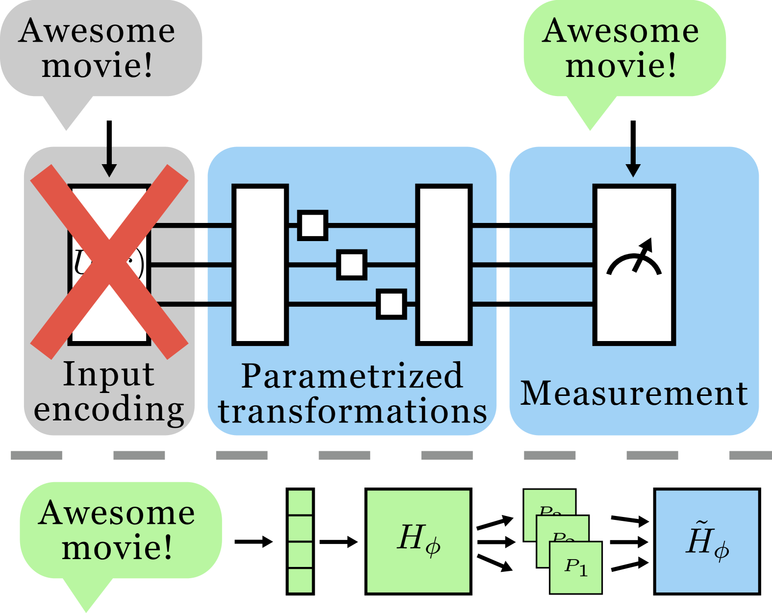
Figure 1: (Top) Schema of a flipped model: data is represented as a measurement avoiding input encoding. (Bottom) The proposed input-to-measurement mapping: data is vectorized, mapped to a Hamiltonian via outer product, decomposed into a small number of Pauli strings, and recomposed into a simplified Hamiltonian

Quantum machine learning is an offshoot of quantum computing that seeks to extend its advantages to data-driven methods. The leading paradigm revolves around variational quantum circuits (VQCs), quantum algorithms whose parameters can be adjusted with classical optimization to solve a specific problem (Cerezo et al., 2021). This approach is sometimes referred to as quantum neural networks given the similarities with the classical counterpart (Farhi and Neven, 2018; Killoran et al., 2019). Prior works have found some evidence that QML algorithms can offer improvements over their classical analogues in terms of capacity (Abbas et al., 2021), expressive power (Du et al., 2020), and generalization (Caro et al., 2022).

Despite the advancements of VQCs, a large-scale demonstration of advantage - the ability of a quantum computer to solve a problem faster, with fewer resources or better performance than any classical counterpart - remains out of reach for QML algorithms. Current quantum machines, referred to as Noisy Intermediate-Scale Quantum (NISQ) devices (Preskill, 2018), are restricted both in size and complexity of the operations they can perform (Zaman et al., 2023). Qubits, the basic units of quantum computation, are hard to maintain in a state useful for computation, and scaling quantum processors to a size suitable for QML remains a significant challenge. Moreover, the widespread use of dense and unstructured vector representations in modern machine learning architectures (Bengio et al., 2000) makes their translation into quantum equivalents challenging. Specifically, the processes of loading data onto a quantum device, known as encoding, and extracting results from it, referred to as measurement, can scale rapidly in terms of qubit requirements or computational costs (Schuld and Killoran, 2022). These costs may grow prohibitively with input size, potentially negating any quantum advantage. As a result, researchers are often forced to down-scale their experiments making it unclear whether these findings generalize at larger scales (Bowles et al., 2024; Mingard et al., 2024).

Motivated by these limitations, we propose a scheme to efficiently encode and measure classical data from quantum devices and demonstrate its effectiveness across different tasks. The method we propose is a specific instance of a flipped model (Jerbi et al., 2024), a type of circuit which encodes data as the observable of a quantum circuit rather than as a quantum state, effectively bypassing the need for input encoding (Figure 1). From a linear algebra perspective, this corresponds to learning a vector representation of the classification problem and using the input data to compute projections of this vector. The magnitude of these projected vectors is then used to make predictions. In quantum-mechanical terms, unstructured input data is mapped onto Pauli strings which are then combined to construct a Hamiltonian. The classifier prediction is obtained as the expectation value of this Hamiltonian. We improve over the standard flipped model by providing a mapping from inputs to observables that achieves a favourable logarithmic qubit and gate complexity relative to the input dimensionality (Figure 1). We also introduce two variants that trade some classification performance in exchange for smaller model size and better sample complexity, respectively. Crucially, the scaling exhibited by these models allows them to be executed on quantum devices and simulated on classical hardware at scales already meaningful for NLP tasks. In brief, this paper provides the following contributions:

1. A novel encoding scheme achieving logarithmic qubit and gate complexity;

2. Variants of this scheme with different performance-cost tradeoffs;

3. A thorough evaluation of our scheme on text and image classification tasks, against established quantum and classical baselines.

2 Background

Quantum computers differ fundamentally from classical computers, utilizing the principles of quantum physics rather than binary logic implemented by transistors. For readers unfamiliar with the topic, in Appendix A we offer a brief introduction to the notation and formalize the concepts of qubit, gate, measurement, and Pauli decomposition. In this section, we instead discuss how these devices have been used to tackle machine learning problems, as well as their limitations.

2.1 Data encoding

The first step for quantum-based ML algorithms is state preparation, the process of representing input data as quantum states. Most algorithms share similarities in how they achieve this (Rath and Date, 2023). The choice of encoding severely impacts the runtime of the circuit as well as its expressivity (Sim et al., 2019). Basis encoding is the simplest representation analogous to classical bits. An $n$-element bit string $\begin{bmatrix}x_{1}&x_{2}&\ldots&x_{n}\end{bmatrix}$ is represented in the basis states of $n$ qubits as $\bigotimes_{i=1}^{n}\ket{x_{i}}=\ket{x_{1}\ldots x_{n}}$ (e.g. $011$ is represented as $\ket{011}$). This representation requires $\mathcal{O}(n)$ qubits. Angle encoding represents continuous data as the phase of qubits. A set of $n$ continuous variables $\begin{bmatrix}x_{1}&x_{2}&\ldots&x_{n}\end{bmatrix}$ can be represented over $n$ qubits as $\bigotimes_{j=1}^{n}R_{\hat{\sigma}}(x_{j})\ket{0}$ with $R_{\hat{\sigma}}(x)=e^{-ix{\hat{\sigma}}}$ a so-called rotation gate, and ${\hat{\sigma}}$ a Pauli matrix $X,Y$ or $Z$ that specifies the rotation axis. Amplitude encoding represents a vector of $N=2^{n}$ values $\begin{bmatrix}x_{1}&x_{2}&\ldots&x_{N}\end{bmatrix}$ over $n$ qubits as $\sum_{i=0}^{N-1}x_{i}\ket{i}$, where $\{\ket{i}\}_{i=1}^{N}$ corresponds to the canonical orthonormal basis written in a binary representation.

There is a trade-off between ease of encoding and qubit count: basis and angle encoding use $\mathcal{O}(n)$ gates for $\mathcal{O}(n)$ values over $\mathcal{O}(n)$ qubits, while amplitude encoding handles $N$-dimensional inputs but needs $\mathcal{O}(N)$ gates over $\mathcal{O}(n)$ qubits, an exponential increase in input size but also gates. Angle encoding strategies often embed multiple features onto the same qubit to reduce qubit usage, effectively a form of pooling (Pérez-Salinas et al., 2020; Du et al., 2020). Amplitude encoding, on the other hand, is often performed using easy-to-prepare quantum states to mitigate its gate complexity (Ashhab, 2022; Du et al., 2020). In text-related tasks, encoding schemes typically encode words over a set number of qubits (Wu et al., 2021; Lorenz et al., 2021), while in image tasks, pixel values are directly encoded as angles or amplitudes (Cong et al., 2019; Wei et al., 2022).

2.2 Variational quantum circuits

Once data has been encoded in a quantum computer, it is processed by a quantum circuit to obtain a prediction. One of the leading paradigms for QML revolves around VQCs (also called quantum ansätze, or parametrized quantum circuits), a type of circuit where the action of gates is controlled by classical parameters. The training loop of a VQC closely resembles that of classical neural networks (Cerezo et al., 2021): input data is encoded in the quantum device as a quantum state, several layers of parametrized gates transform this state, a prediction is obtained via quantum measurement, and finally, a specialized but classical optimizer  (Wierichs et al., 2022) computes a loss and updates the parameters. VQCs have shown better convergence during training (Abbas et al., 2021) as well as better expressive power (Du et al., 2020) compared to neural networks of similar size.

Several VQC-based equivalents of classical architectures have been proposed such as auto-encoders (Romero et al., 2017), GNNs (Dallaire-Demers and Killoran, 2018), and CNNs (Cong et al., 2019; Henderson et al., 2020). Quantum NLP works have focused on implementing VQCs with favourable inductive biases for text, such as quantum RNNs (Bausch, 2020; Li et al., 2023), quantum LSTMs (Chen et al., 2022), and quantum attention layers (Cherrat et al., 2022; Shi et al., 2023; Zhao et al., 2024), with recent works showcasing applicability of these methods at scales meaningful for NLP applications (Xu et al., 2024)

2.3 Quantum Machine Learning limitations

Despite these achievements, QML applications have yet to demonstrate a practical quantum advantage. Firstly, NISQ devices are limited in terms of the number of qubits in a single device, connectivity between the qubits, noise in the computation, and coherence time (Zaman et al., 2023; Anschuetz and Kiani, 2022). Secondly, quantum devices have fundamental difficulties in dealing with the dense and unstructured vector representations around which ML revolves: loading (or encoding) data into a quantum state either requires a large number of qubits (for angle and basis encoding) or a prohibitive amount of gates (for amplitude encoding). Efficient methods for amplitude encoding (Ashhab, 2022; Wang et al., 2009) incur trade-offs in the expressivity of vectors that have not been explored sufficiently in the context of QML. Moreover, measurement is an expensive process extracting only one bit of information per qubit measured. Extracting a real-valued vector from a quantum computer generally requires exponentially many measurements (Schuld and Petruccione, 2021). As a result, many current QML experiments are limited in both scale and scope in order to fit within the constraints of NISQ devices and simulators. Small datasets, typically consisting of only a few hundred samples, are often used (Senokosov et al., 2024; Li et al., 2023; Liu et al., 2021; Chen, 2022). Additionally, aggressive dimensionality reduction is commonly performed to reduce data to just a few dozen features (Bausch, 2020; Zhao et al., 2024). In contrast, even "small" classical neural networks by modern standards are several orders of magnitude larger in terms of parameters, dataset size, and representation dimensionality (Mingard et al., 2024). These limitations have raised concerns about the applicability of QML results to larger, more complex tasks. Some question whether the observed performance is due to the quantum model itself or the upstream pre-processing (Chen et al., 2021), while others highlight the difficulty of generalizing these results to larger datasets and the challenges of fair benchmarking (Bowles et al., 2024; Mingard et al., 2024). Several other challenges remain, including barren plateaus (Larocca et al., 2024), development of efficient optimization algorithms for VQCs (Wiedmann et al., 2023), and error correction (Chatterjee et al., 2023).

To mitigate the data loading and read-out challenges, the flipped model has been recently introduced (Jerbi et al., 2024), where quantum resources are only required during training, while inference can happen classically. Although flipped models on NISQ devices are classically simulatable and thus cannot yet achieve quantum advantage, they hold significant promise when combined with shadow techniques (Huang et al., 2020; Song et al., 2023), which allow the prediction of many quantum system properties from a limited number of measurements. There are theoretically provable instances where shadow-flipped models outperform classical methods under widely-believed cryptography assumptions Gyurik and Dunjko (2022). The guarantees of flipped models, as well as their scalability, warrant their exploration in the context of NLP.

3 Hamiltonian classifier

In the following, we describe a flipped model that improves over previous works by sensibly lowering qubit requirements. To the best of our knowledge, we are the first to apply flipped models to text classification and to provide a thorough evaluation of such methods across multiple datasets, comparing against classical and quantum baselines. We also propose two variants that further reduce model size and sample complexity with minimal impact on performance and extend flipped models to the multi-class scenario.

3.1 Fully-parametrized Hamiltonian (HAM)

Our Hamiltonian classifier takes as input a sequence of embeddings $x=\begin{bmatrix}x_{1}&x_{2}&\ldots&x_{s}\end{bmatrix},\,x_{i}\in\mathbb{R}^{d}$ and outputs a prediction probability $f_{\theta,\phi}$, a real number representing the estimated class the input belongs to. Similarly to VQCs, gradient descent is used to optimize the classifier parameters $\theta,\phi$ on a given training set X with binary labels y. The classifier can encode embeddings of size at most $N=2^{n}$ with the remaining $N-d$ dimensions padded to $0$. The optimization problem can be summarized as:

$$\argmin_{\theta,\phi}\frac{1}{|\textbf{X}|} \sum_{x\in\textbf{X},y\in\textbf{y}}\mathcal{L}(f_{\theta,\phi}(x),y),$$ (1)

$$f_{\theta,\phi}(x) \coloneqq\sigma(\psi_{\theta}^{\dagger}H_{\phi}(x)\psi_{\theta})$$ (2)

$$H_{\phi}(x) \coloneqq H_{\phi}^{0}+\frac{1}{s}\sum_{i=1}^{s}x_{i}x_{i}^{\top}$$ (3)

$$\psi_{\theta}\coloneqq U_{\theta}\ket{0}^{\otimes n} =U_{\theta}\begin{bmatrix}1&0&\cdots&0\end{bmatrix}^{\top}.$$ (4)

$H_{\phi}\in\mathbb{R}^{N\times N}$ is the Hamiltonian of our system, and is constructed from embeddings $x$ and a bias term $H_{\phi}^{0}\in\mathbb{R}^{N\times N}$ (Eq. 3). The bias term is a fully parametrized Hermitian matrix, giving more fine-grained control over the Hamiltonian. $U_{\theta}\in\mathbb{C}^{N\times N}$ represents a VQC, and $\psi_{\theta}$ is the result of applying said VQC to the starting state (Eq. 4). The specific choice of VQC is application-dependant and we experiment with three qubit-efficient circuits during hyperparameter tuning, which we discuss in Appendix B. The prediction probability $f_{\theta,\phi}$ is regularized using the sigmoid function $\sigma$ (Eq. 2). Finally, parameters $\theta,\phi$ are optimized classically to minimize the loss function $\mathcal{L}$, the cross entropy. When building $U_{\theta}$ and $\psi_{\theta}$, they are not explicitly represented as dense matrices in classical form. Instead, they are constructed directly on quantum hardware from a manageable set of parameters, avoiding the need for large-scale classical representations. By encoding inputs of size $d\leq N$ over $n$ qubits, we attain logarithmic scaling in the number of qubits and an overall sample complexity that scales quadratically in the embedding size. We expand on this in Section 3.4.

3.2 Parameter-efficient Hamiltonian (PEFF)

The bias term $H_{\phi}^{0}$ of HAM significantly contributes to its parameter count, resulting in a $\mathcal{O}(N^{2})$ scaling. To lower the model size, we experiment with applying a bias term $b_{\phi}\in\mathbb{R}^{d}$ directly to the input embeddings as $\tilde{x}_{i}\coloneqq x_{i}+b_{\phi}$. This term skews the distribution in the vector space while only requiring $\mathcal{O}(d)$ parameters. The Hamiltonian is then constructed as $H_{\phi}(\tilde{x})\coloneqq\frac{1}{s}\sum_{i=1}^{s}\tilde{x}_{i}\tilde{x}$.

Physically implementing the Hamiltonians of HAM and PEFF requires first decomposing them into observables the quantum device can measure and then performing measurements for each observable separately. As we detail in Appendix A, this process is potentially expensive, requiring an exponential number of operations. In the following, we show how the model can be restructured to drastically reduce this cost.

3.3 Simplified Hamiltonian (SIM) variant

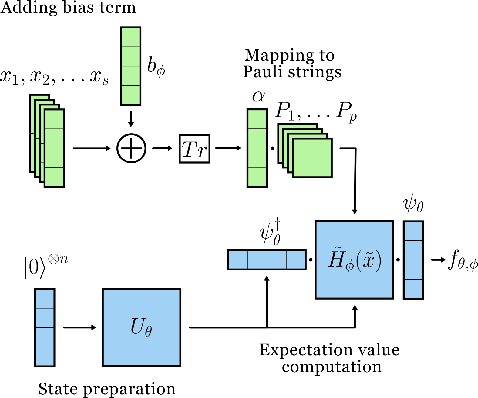
Figure 2: The SIM model at a glance. In green, parts that are stored classically, in blue, parts that can be represented on quantum computers.

To address the computational challenges we describe above, we propose an extension of PEFF that constructs the Hamiltonian from a small number $p$ of Pauli strings, circumventing the need for an expensive decomposition and reducing the number of necessary measurements to $\mathcal{O}(p)$ (Figure 2). More information about Pauli strings can be found in Appendix A. We define $p$ Pauli strings $P_{1},P_{2},\ldots P_{p}\in\mathcal{P}_{n}$ (in practice, they can be chosen at random) and use them to compute the corresponding coefficients $\alpha_{1},\alpha_{2},\ldots\alpha_{p}$ from $H$:

$$\tilde{x} \coloneqq\frac{1}{s}\sum_{i=1}^{s}x_{i}+b_{\phi}$$ (5)

$$H_{\phi}(\tilde{x}) \coloneqq\tilde{x}\tilde{x}^{\top}$$ (6)

$$\alpha_{i} =\frac{1}{2^{n}}\mathrm{Tr}(P_{i}H_{\phi})=\frac{1}{2^{n}}\tilde{x}^{\top}P_{i}\tilde{x}$$ (7)

$$\tilde{H}_{\phi}(\tilde{x}) \coloneqq\sum_{j=1}^{p}\alpha_{j}w_{j}P_{j},$$ (8)

where $w_{j}\in\mathbb{R}$ is a learned parameter that re-weights the effect of Pauli strings. $P_{j}$ and $H_{\phi}$ in Eq. 7 are generally large matrices, but several algorithms exist that side-step the costs of full multiplication by exploiting the structure of the Pauli string (Koska et al., 2024; Hantzko et al., 2024). For this method, we choose to redefine $H_{\phi}$ (Eq. 5 and 6) in a way that allows replacing the expensive matrix-matrix product $P_{i}H_{\phi}$ with two more efficient vector-matrix products $\tilde{x}^{\top}P_{i}\tilde{x}$, thus improving scaling.

To emphasize the underlying transformation, we recast the expectation value computation in SIM:

$$f_{\theta,\phi}(\tilde{x}) =\sigma\Big{(}\frac{1}{2^{n}}\sum_{j=1}^{p}\tilde{x}^{\dagger}P_{j}\tilde{x}w_{j}\psi_{\theta}^{\dagger}P_{j}\psi_{\theta}\Big{)}.$$ (9)

Equation 9 shows that SIM computes a weighted sum of several feature maps $\tilde{x}^{\dagger}P_{j}\tilde{x}$, where the weights are determined by both the learned term $w_{j}$ and the factor $\psi_{\theta}^{\dagger}P_{j}\psi_{\theta}$. These two terms concur to select the feature maps most relevant for solving the problem. During our exploration, we observe that removing $w_{j}$ significantly degrades performance. We speculate this occurs because $\psi_{\theta}^{\dagger}P_{j}\psi_{\theta}$ is constrained to the range $[-1,1]$, whereas the presence of $w_{j}$ introduces a notion of magnitude that facilitates training. A related approach is discussed in Huang and Rebentrost (2024), which focuses on improving variational strategies rather than directly addressing the challenges of input encoding. We believe that these two methods could be synergistically combined to further reduce overall computational costs.

All proposed methods output a prediction probability $f_{\theta,\phi}$ to be interpreted as a binary label. We can extend this to a scenario with $c$ distinct classes by using a one-vs-many approach: either $U_{\theta}$, $b_{\phi}$ or $w$ can be tied to a specific class to obtain a class-specific discriminator. We choose a setup that learns $c$ distinct re-weightings $w_{1},w_{2},\ldots w_{c}$ and build $c$ separate Hamiltonians $\tilde{H}^{1}_{\phi},\tilde{H}^{2}_{\phi},\ldots\tilde{H}^{c}_{\phi}$ so that each one discriminates a single class. For class $k$, we have $H^{k}_{\phi}(\tilde{x})\coloneqq\sum_{j=1}^{p}\alpha_{j}w^{k}_{j}P_{j}$. Parameter count scales as $\mathcal{O}(c)$, although different choices of parameter sharing strongly affect the final number. Since our setup learns different weights for the same Pauli strings across classes, expectation values on a real quantum device can be computed only once and then post-processed to obtain probabilities for all classes.

3.4 Complexity analysis

In this section, we compare the theoretical qubit count, gate complexity, and sample complexity of our classifier with other established models from the literature. We consider a subset of implementations from the literature that we consider representative of the current discourse. Our three variants all achieve a qubit count that scales as the logarithm of the input dimensionality. This is determined by the number of qubits required to encode a large enough Hamiltonian. For our models, gate complexity depends entirely on the chosen circuit $U_{\theta}$. The ansätze we consider throughout our experiments result in a linear or quadratic scaling. Sample complexity, defined as the total number of Pauli strings to measure in order to obtain a prediction, both HAM and PEFF necessitate a full evaluation of the Hamiltonian, resulting in a complexity of $\mathcal{O}(4^{n})$. Since $4^{\log_{2}(d)}=2^{\log_{2}(d^{2})}$, we conclude that the sample complexity is $\mathcal{O}(d^{2})$. Notably, SIM combines the logarithmic scaling in qubit and gate complexity of the other variants with a constant sample complexity made possible by simplifying the Hamiltonian, making it a strong candidate for practical implementation on NISQ devices. The full comparison is shown in Table 1. For readability, we omit the precision term arising when running these methods on quantum hardware. All models incur an additional $1/\epsilon^{2}$ term in sample complexity, where $\epsilon$ is the desired precision.

Model	Reference	Qubit count	Gate complexity	Sample complexity
QCNN	Henderson et al. (2020)	$\mathcal{O}(d)$	$\mathcal{O}(d^{2})$	$\mathcal{O}(2^{d})$
	Cong et al. (2019)	$\mathcal{O}(\log d)$	$\mathcal{O}(d+l\log d)$	$\mathcal{O}(p)$
QLSTM	Chen et al. (2022)	$\mathcal{O}(d)$	$\mathcal{O}(ld)$	$\mathcal{O}(d)$
QNN	Farhi and Neven (2018)	$\mathcal{O}(d)$	$\mathcal{O}(l)$	$\mathcal{O}(1)$
	Mitarai et al. (2018)	$\mathcal{O}(d)$	$\mathcal{O}(ld)$	$\mathcal{O}(1)$
	Schuld et al. (2020)	$\mathcal{O}(\log d)$	$\mathcal{O}(d+l\log d)$	$\mathcal{O}(1)$
HAM	Ours	$\mathcal{O}(\log d)$	$\mathcal{O}(l\log d)\text{ or }\mathcal{O}(l\log(d)^{2})$	$\mathcal{O}(d^{2})$
PEFF	Ours	$\mathcal{O}(\log d)$	$\mathcal{O}(l\log d)\text{ or }\mathcal{O}(l\log(d)^{2})$	$\mathcal{O}(d^{2})$
SIM	Ours	$\mathcal{O}(\log d)$	$\mathcal{O}(l\log d)\text{ or }\mathcal{O}(l\log(d)^{2})$	$\mathcal{O}(p)$

Table 1: Theoretical scaling comparison of various VQCs, with $d$ input size, $l$ number of layers, and $p$ number of Pauli strings to measure (defined as a hyperparameter).

4 Experiments

4.1 Datasets & Pre-processing

To evaluate the capabilities of our models, we select a diverse set of tasks encompassing both text and image data, covering binary and multi-class scenarios. To facilitate replicability, our scripts automatically download all datasets on the first run.

Text datasets We first consider the GLUE Stanford Sentiment Treebank (SST) dataset as obtained from HuggingFace (Socher et al., 2013; Wang et al., 2019). It consists of $\sim 70k$ single sentences extracted from movie reviews whose sentiment (positive/negative) was annotated by 3 human judges. We then evaluate our method on the IMDb Large Movie Review Dataset (Maas et al., 2011) containing $50k$ highly polar movie reviews. We also consider the AG News (Zhang et al., 2015) classification task as a benchmark for our multi-class model. AG News consists of $\sim 128k$ news articles divided by topic (world, sports, business, sci/tech). These are commonplace datasets reasonably close to real-world applications. For text datasets, we remove all punctuation, lowercase all text, tokenize with a whitespace strategy, and finally embed tokens with word2vec to obtain a sequence $x$. The resulting embedding has size $d=300$ and requires $n=9$ qubits to be represented in our methods.

Image datasets As a sanity check, we consider a binary version of MNIST which only includes digits 0 and 1. We then consider Fashion-MNIST (Xiao et al., 2017), a dataset of $60k$ grayscale images of clothes subdivided into 10 classes. Feeding images directly to our models results in $d=784$ and $n=10$. We further experiment on a binarized version of the CIFAR-10 dataset (Krizhevsky, 2012) we name CIFAR-2 obtained by grouping the original ten classes into two categories: vehicles and animals. The $32\times 32$ RGB images result in $d=1024$ features over $n=10$ qubits. We also note that no further pre-processing or dimensionality reduction is performed to preserve the original properties of the images. MNIST and Fashion-MNIST representations are not sequential and therefore are considered by our model as a special case with $s=1$, while in CIFAR-2 each channel is considered as a different element of a sequence with $s=3$.

	SST2			IMDb			AG News
Model	# Params	Train	Test*	# Params	Train	Test	# Params	Train	Test
LOG	301	84.7	80.4	301	85.8	85.5	1204	90.1	89.2
MLP	180901	97.5	80.2	180901	88.1	85.8	40604	90.2	89.1
LSTM	241701	97.8	84.4	241600	99.3	88.4	242004	91.5	90.5
RNN	40301	89.6	80.1	60501	79.7	78.1	40604	88.8	88.1
CIRC	923	85.2	80.1	923	86.1	85.8	2387	89.7	89.2
QLSTM	2766	89.9	84.4	4679	76.8	67.9	3582	87.2	86.7
HAM	130854	91.2	82.3	130926	91.0	88.1	-	-	-
PEFF	410	81.8	80.0	410	84.0	83.8	-	-	-
SIM	1338	80.6	79.0	1410	86.0	85.3	4416	89.4	88.6

Table 2: Accuracies across text datasets. Results are averaged over $10$ runs or (*) run achieving lowest training loss.

4.2 Baselines

We compare our classifiers (HAM, PEFF, SIM) with three quantum baselines: a QLSTM (Chen et al., 2022), a QCNN (Cong et al., 2019), and a simple circuit ansatz (CIRC). QLSTM and QCNN have been adapted from implementations of the original papers. CIRC is our implementation and consists of an amplitude encoding for the input, the same hardware-efficient ansätze of HAM, and a linear regression on the circuit’s output state. Note that running CIRC in practice would require state tomography, this setup is therefore not meant to be efficient or scalable but rather to give a best-case scenario of a VQC of similar complexity to our classifier. We also compare with out-of-the-box classical baselines: a multi-layer perception (MLP), a logistic regression (LOG), an RNN, an LSTM, and a CNN. MLP and LOG act on the mean-pooled embedding of the sequence.

4.3 Experimental setting

We first perform a random search on hyperparameters such as learning rate, batch size, number of qubits, and number of layers to identify the best configuration of each architecture. For the sake of brevity, a more detailed discussion is moved to Appendix B. After identifying the best hyperparameters, we train $10$ models for each architecture with randomized seeds on the original training split and average their performance on the test split. The only exception is the SST2 dataset for which no test set is provided. In this case, we select the run achieving the lowest training loss and submit it to GLUE’s website to get a test score. Appendix LABEL:sec:apn-abl shows additional experiments in which we further investigate architectural choices such as bias, state preparation, and number of Pauli strings. With the exception of QCNN which is implemented in PennyLane, all quantum operations are simulated in PyTorch as it allows batching several Hamiltonians thus enabling efficient training. We do not simulate noise in order to assess the performance of our approach under an ideal scenario. For all tasks, we use a cross-entropy loss during training.

4.4 Results

In Tables 2 and 3, we report train and test accuracy for the text and image datasets respectively. MNIST2 is omitted for brevity since all models successfully achieve perfect scores. This validates our setup and confirms that HAM, PEFF, and SIM learn correctly. In the SST2 task, HAM performs competitively with baseline methods using a similar number of parameters, outperforming simpler models like LOG, MLP and RNN, and ranking just below the LSTM and QLSTM. AG News and IMDb turn out to be easier tasks, with SIM achieving scores comparable to the baselines and accuracy being high for all models. CIFAR2 proves to be a hard task, likely due to the images being coloured rather than grayscale and having a higher resolution: while HAM and PEFF score relatively higher than the LOG baseline, SIM underperforms, possibly due to its relatively simple decision boundary. We speculate that a higher number of Pauli strings would narrow this gap, as more complex transformations would increase the capacity of the model. On Fashion, SIM performs better than LOG but worse than other baselines. Notably, CIRC achieves relatively high performance. Across tasks, PEFF and SIM attain performance comparable with the baseline despite the low parameter count. PEFF confirms our intuition that simply skewing points in the embedding space can substitute the bulky bias term over the whole Hamiltonian, while SIM confirms that performance can be retained even with a Hamiltonian composed of few Pauli strings. The high parameter count of HAM in MNIST2 and CIFAR2 is necessary to encode full-size images, resulting in large Hamiltonians. Across quantum models, we find no clear link between entangling circuits and performance; non-entangling baselines often perform best, aligning with prior findings (Bowles et al., 2024).

We perform additional experiments in Appendix LABEL:sec:apn-abl and find evidence that the number of Pauli strings is strongly linked with better performance. Specifically, larger models with more Pauli strings exhibit higher accuracy and more stable training dynamics (Figure 3). Notably, between 500 and 1000 Pauli strings are already sufficient to match the performance of classical baselines on most tasks. This result aligns with our expectations, as increasing the number of Pauli strings enables the model to capture more complex features, as demonstrated in Eq. 9. Furthermore, we find that removing the bias term significantly worsens performance, underlining the importance of this component.

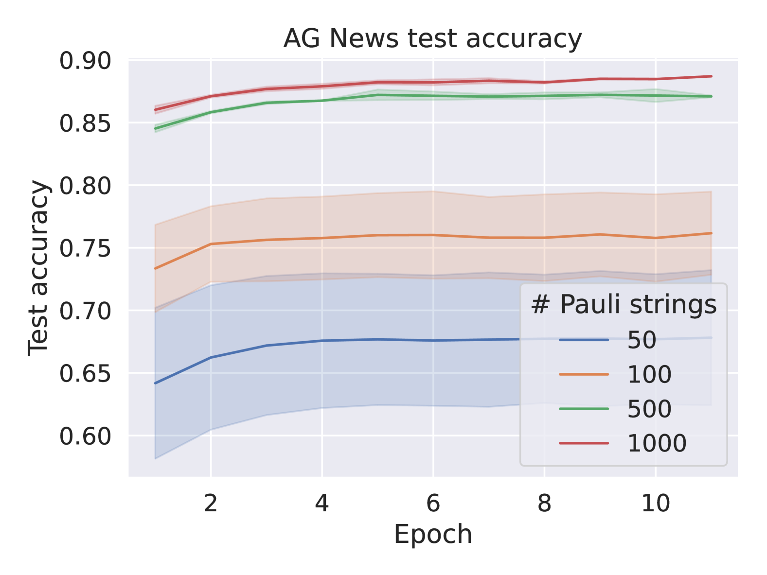
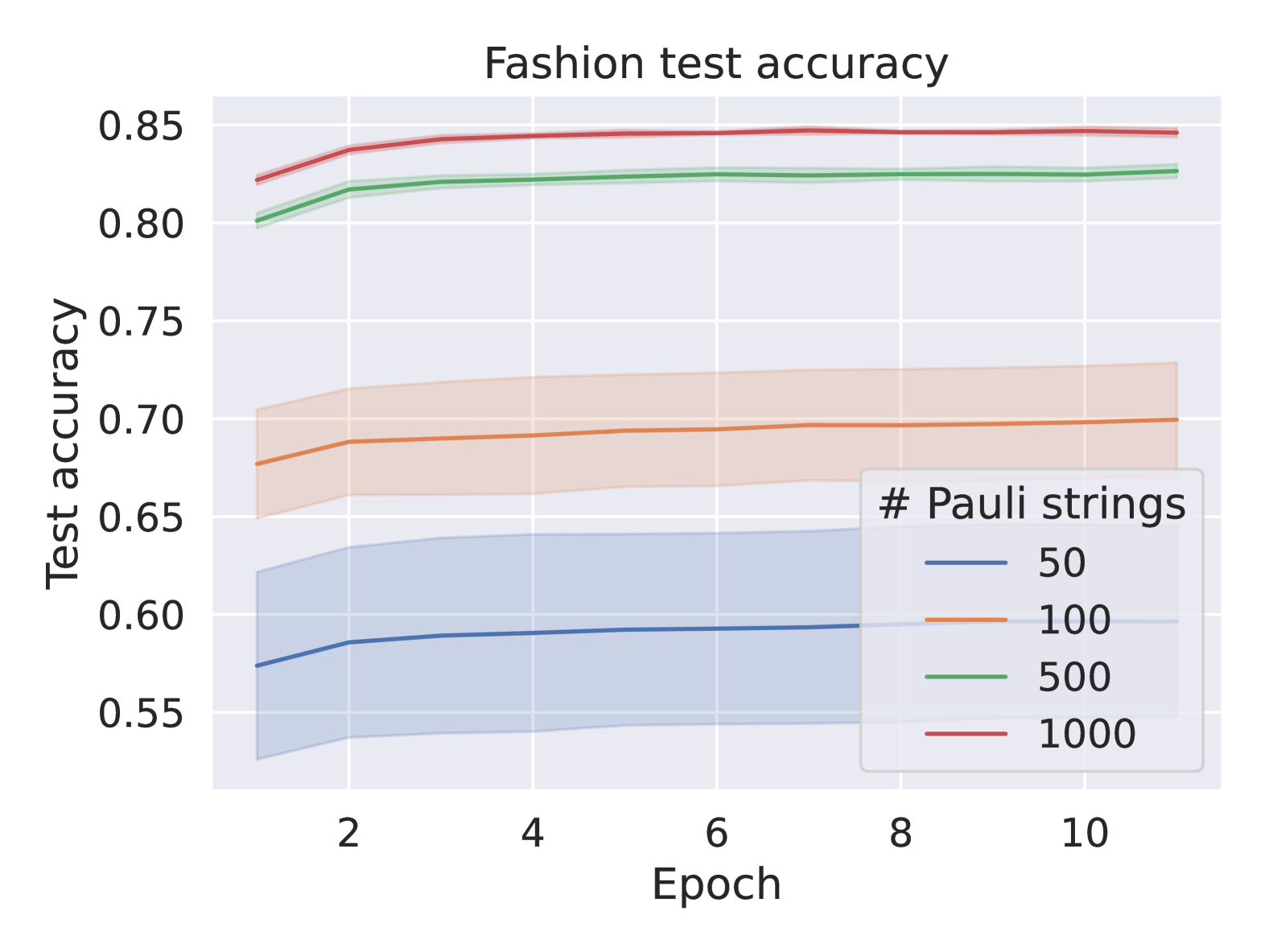
Figure 3: Performance on the test sets for different number of Pauli strings in the SIM model. First $10$ epochs out of $30$ shown.

	CIFAR2			Fashion
Model	Params	Train	Test	Params	Train	Test
LOG	1025	73.9	72.9	1025	85.5	83.5
MLP	112701	89.0	83.4	89610	87.9	85.8
CNN	75329	96.3	94.1	130250	95.4	90.7
CIRC	2081	85.1	84.6	11094	89.2	86.5
QCNN	169	84.9	84.7	558	76.7	76.3
HAM	523818	89.6	81.0	-	-	-
PEFF	1056	79.3	78.7	-	-	-
SIM	2156	68.9	68.2	10934	87.6	84.4

Table 3: Accuracies across image datasets. Results are averaged over $10$ runs.

	# Params	Train	Test*
HAM	130854	91.2	82.3
PEFF	410	81.8	80.0
SIM	9410	84.5	80.1
STATEIN	130854	92.0	80.2
NOBIAS	38	70.0	71.9

Table 4: Accuracies of additional variants on SST2. Results are averaged over $10$ runs or (*) run achieving best train accuracy.

5 Discussion and future work

This work extends the scalability of flipped models and makes it possible to process significantly larger inputs. Moreover, it demonstrates their importance as a viable quantum method for NLP tasks. The proposed HAM design encodes input data directly as a measurement, obtaining performance comparable with other specialized models. The PEFF variant reduces its parameter complexity, and the SIM variant additionally reduces its sample complexity, offering a scheme that may be more efficiently implemented on quantum hardware. Notably, our method already scales well enough to allow meaningful studies on large datasets using simulators. The Hamiltonian classifier is presently a proof of concept meant to illustrate a novel input scheme for quantum devices with the ultimate goal of expanding the tools available to QML researchers. Future works could characterize the effectiveness of our approach on even larger problems and its integration with existing classical pipelines. Other studies could consider local strings in conjunction with classical shadows techniques to lower sample complexity. A way of learning more complex functions could be to stack several layers of Hamiltonian encoding, possibly performing nonlinear transformations. On the same thread, our Hamiltonian classifier could be reformulated as a feature extractor, allowing in to be integrated into hybrid quantum-classical pipelines. Other directions deserving a paper of their own are noise simulation and physical implementations on real quantum hardware.

Limitations

This work does not evaluate HAM and PEFF in multi-class scenarios. Although a one-vs-many approach similar to SIM could be applied, simulating a separate Hamiltonian for each class would demand substantial computational resources. Instead, we prioritized comprehensive hyperparameter search and experimentation on a wider selection of datasets to provide a better assessment of these methods’ performance.

We are limited to a small number of qubits and Pauli strings due to constraints in our implementation of the Hamiltonians. While increasing the qubit count of our system could enhance performance, a key strength of our approach is that it does not require a large number of qubits to operate effectively at scales already meaningful for NLP tasks.

Although our results do not yet match state-of-the-art NLP models, this work highlights the potential of large-scale quantum architectures, marking an important step toward practical applications. Theoretical findings on flipped models suggest that realizing a definitive advantage will require more advanced quantum devices than those presently available Jerbi et al. (2024), making it unrealistic to expect these models to surpass classical counterparts at this stage. Consistent with prior efforts such as Xu et al. (2024), our emphasis remains on scalability rather than immediate performance parity with classical methods.

Noisy simulations and real hardware implementation fall outside the scope of this work, as the current model was not designed with noise resilience in mind.

Appendix A Quantum computing fundamentals

Quantum computers are conceptually and physically different devices from classical computers. Instead of basing their logic on binary data representations implemented by transistors, they utilize the rules of quantum physics as a substrate for computation. For this reason, in what follows we describe the building blocks of quantum computation.

Dirac notation Quantum computing makes extensive use of Dirac notation (also called bra-ket notation) to simplify the representation of linear transformations which are commonplace in the theory. The fundamental elements of this notation are bras and kets. A ket, denoted as $\ket{\psi}$, represents a column vector $\psi$ in a Hilbert space. A bra, denoted as $\bra{\phi}$, represents instead a vector in the dual space (the complex conjugate transpose of a ket). The inner product of two vectors $\phi$ and $\psi$, which results in a scalar, is written as $\braket{\phi}{\psi}$. Conversely, the outer product $\ket{\psi}\bra{\phi}$, forms a matrix or an operator.

Quantum systems The basic unit of information in a quantum computer is a two-dimensional quantum bit (qubit) which is mathematically modelled by a normalized column vector, the state vector, in a two-dimensional vector space equipped with an inner-product, or Hilbert space. A state vector is usually expressed concisely in Dirac notation as $\ket{\psi}=\begin{bmatrix}\alpha&\beta\end{bmatrix}^{\top}\in\mathbb{C}^{2}$. We say that a qubit $\ket{\psi}\coloneqq\alpha\ket{0}+\beta\ket{1}$ is in a coherent quantum superposition of two orthonormal basis states $\ket{0}\coloneqq\begin{bmatrix}1&0\end{bmatrix}^{\top}$ and $\ket{1}\coloneqq\begin{bmatrix}0&1\end{bmatrix}^{\top}$, such that the complex coefficients in the basis expansion satisfy normalization constraint $|\alpha|^{2}+|\beta|^{2}=1$. This constraint originates from physics: in order to extract any information from a quantum state, we need to measure it in a chosen basis, which destroys the superposition in the measured basis by projecting the state $\ket{\psi}$ on one of the basis elements. If we measure state $\ket{\psi}$ in the $\{\ket{0},\ket{1}\}$ basis, we get outcome "$0$" with probability $|\alpha|^{2}$ and the post-measurement state becomes $\ket{0}$, and respectively, we get "$1$" with probability $|\beta|^{2}$ and post-measurement state $\ket{1}$.

Multi-qubit systems In order to model a quantum system with multiple qubits, we use the so-called Kronecker product ($\otimes$) to combine many individual state vectors into a single larger one. An $n$-qubit system can be represented by a vector of size $N=2^{n}$, $\ket{\psi_{1}\dots\psi_{n}}\coloneqq\ket{\psi_{1}}\otimes\dots\otimes\ket{\psi_{n}}$. In a chosen basis, the entries of this vector describe the probability of observing that outcome. Many QML approaches aim to gain a quantum advantage by manipulating only a few qubits to access an exponentially large Hilbert space. To give an example, if two qubits $\ket{\psi_{1}}$ and $\ket{\psi_{2}}$ are both initialized in $(\ket{0}+\ket{1})/\sqrt{2}$, the joint state is given by an equal superposition of all the possible $n=2$ bit string vectors

$$\begin{split}\ket{\psi_{1}}\otimes\ket{\psi_{2}}=\frac{\ket{00}+\ket{01}+\ket{10}+\ket{11}}{2}.\end{split}$$

In this setup, measurement can performed separately on each qubit, resulting in a $n$-element bitstring.

Quantum circuits Quantum computation is achieved by manipulating qubits. This is done using quantum gates. Any $n$-qubit gate can be represented as a unitary matrix $U\in\mathbb{C}^{N\times N}$ which acts on the $n$-qubit input state $\ket{\psi}$ via the usual matrix-vector multiplication, giving output $U\ket{\psi}$. Intuitively, quantum gates can be considered as rotations that conserve the length of a state vector. A sequence of gates applied on one or many qubits is called a quantum circuit. By construction, unitary circuits perform linear operations. Non-linear computation requires workarounds like running the computation on a larger Hilbert space and measuring output qubits in a subspace or re-uploading input data (Killoran et al., 2019; Pérez-Salinas et al., 2020; Subasi et al., 2023).

Pauli decomposition A concise way of expressing multiple measurements on multiple qubits over multiple bases is through a so-called Hamiltonian. A Hamiltonian $H$ for an $n$-qubit system is a Hermitian matrix of size $2^{n}\times 2^{n}$. The result of a measurement of a state $\psi$ with a specific Hamiltonian $H$ can be expressed as $\bra{\psi}H\ket{\psi}$, which is the expectation value of this measurement. The $2\times 2$ Pauli matrices, $\mathcal{P}=\{X,Y,Z,I\}$, or more generally multi-body Pauli operators, also called Pauli strings, $\mathcal{P}_{n}=\{\bigotimes_{i=1}^{n}O_{i}|O_{i}\in\mathcal{P}\}$ form a basis for Hermitian matrices of dimension $2^{n}\times 2^{n}$. Consequently, any Hamiltonian can be expressed as a linear combination of Pauli strings:

$$H=\sum_{i}\alpha_{i}P_{i}\quad\text{where}\quad\alpha_{i}\in\mathbb{R}\quad\text{and}\quad P_{i}\in\mathcal{P}_{n}.$$

This decomposition results in $\mathcal{O}(4^{n})$ unique Pauli strings, each representing a physical property that can be measured using quantum devices. Generic Hamiltonians are expensive to decompose and measure due to the exponential number of Pauli strings. For this reason, in VQC settings, typical Hamiltonians are constructed from a polynomial number of Pauli strings.

Appendix B Hyperparameter tuning

For each architecture and for each dataset in our evaluation, we perform a randomised search for the best parameters: we randomly select $50$ configurations, train them on the task and evaluate their performance on the development set. To avoid overfitting, we perform early stopping on the training if development loss does not decrease for five consecutive epochs. Troughout all experiments, we utilize the Adam optimizer provided by PyTorch. Since our largest model HAM has at most $\sim 500k$ parameters (dictated by the embedding space), we limit the random search to configuration with less-than or equal number of parameters to ensure a fair comparison. In practice, we find RNNs, LSTMs and CNNs perform very well with as low as $40k$ parameters. What follows is a list of all hyperparameters we evaluated:

• Batch size: $[64,128,256]$;

• Learning rate: $[10^{-2},10^{-3},10^{-4}]$;

• Hidden size: For RNNs and LSTMs, the size of the hidden representation $[100,300,500]$;

• Layers: For RNNs and LSTMs, the number of layers of the recurrent block $[1,4,8]$. For MLP, the total number of layers including input and output $[3,4,5]$. For CNNs, the total number of convolutional layers $[3,4,5]$. For HAM, PEFF, SIM and CIRC, the number of repeated applications of the ansatz, analogous to the number of layers $[8,16,32]$;

• Channels: For CNNs, the number of output channels of each convolutional layer $[8,16,32,64,128]$;

• Kernel size: For CNNs, the kernel dimension of each convolutional layer $[3,5,7]$;

• Circuit: The ansatz $U_{\theta}$ used to prepare state $\psi$. We experiment with three hardware-efficient ansätze inspired by circuits from Sim et al. (2019) and illustrated in Figure LABEL:fig:ansz. These ansätze are designed to explore different levels of entanglement (the quantum counterpart of correlation) and gate complexity. The first is a non-entangling circuit composed of single-qubit rotations, exhibiting linear complexity with respect to the number of qubits. The second is an entangling circuit arranged in a ring configuration, also scaling linearly in gate count. The third is an all-to-all entangling circuit, which scales quadratically. $[\texttt{Baseline, Ring, All-to-all}]$.

• # Pauli strings: For SIM, the number of Pauli strings composing the Hamiltonian $[50,100,500,1000]$.

Tables LABEL:tab:hyp-baseline and LABEL:tab:hyp-ham shows the final selection of best-performing hyperparameters used in the main experiment of Section 4.3.

(a)

(b)

References

- Abbas et al. (2021) Amira Abbas, David Sutter, Christa Zoufal, Aurelien Lucchi, Alessio Figalli, and Stefan Woerner. 2021. The power of quantum neural networks. Nature Computational Science, 1(6).
- Anschuetz and Kiani (2022) Eric R Anschuetz and Bobak T Kiani. 2022. Quantum variational algorithms are swamped with traps. Nature Communications, 13(1):7760.
- Ashhab (2022) Sahel Ashhab. 2022. Quantum state preparation protocol for encoding classical data into the amplitudes of a quantum information processing register’s wave function. Phys. Rev. Res., 4:013091.
- Bausch (2020) Johannes Bausch. 2020. Recurrent quantum neural networks. In Advances in Neural Information Processing Systems 33: Annual Conference on Neural Information Processing Systems 2020, NeurIPS 2020, December 6-12, 2020, virtual.
- Bengio et al. (2000) Yoshua Bengio, Réjean Ducharme, and Pascal Vincent. 2000. A neural probabilistic language model. In Advances in Neural Information Processing Systems 13, Papers from Neural Information Processing Systems (NIPS) 2000, Denver, CO, USA, pages 932–938. MIT Press.
- Biamonte et al. (2017) Jacob Biamonte, Peter Wittek, Nicola Pancotti, Patrick Rebentrost, Nathan Wiebe, and Seth Lloyd. 2017. Quantum machine learning. Nature, 549(7671):195–202.
- Bowles et al. (2024) Joseph Bowles, Shahnawaz Ahmed, and Maria Schuld. 2024. Better than classical? the subtle art of benchmarking quantum machine learning models. Preprint, arXiv:2403.07059.
- Camps et al. (2021) Daan Camps, Roel Van Beeumen, and Chao Yang. 2021. Quantum fourier transform revisited. Numerical Linear Algebra with Applications, 28(1):e2331.
- Caro et al. (2022) Matthias C. Caro, Hsin-Yuan Huang, M. Cerezo, Kunal Sharma, Andrew Sornborger, Lukasz Cincio, and Patrick J. Coles. 2022. Generalization in quantum machine learning from few training data. Nature Communications, 13(1):4919.
- Cerezo et al. (2021) M. Cerezo, Andrew Arrasmith, Ryan Babbush, Simon C. Benjamin, Suguru Endo, Keisuke Fujii, Jarrod R. McClean, Kosuke Mitarai, Xiao Yuan, Lukasz Cincio, and Patrick J. Coles. 2021. Variational quantum algorithms. Nature Reviews Physics, 3(9).
- Chatterjee et al. (2023) Avimita Chatterjee, Koustubh Phalak, and Swaroop Ghosh. 2023. Quantum error correction for dummies. In Proceedings - 2023 IEEE International Conference on Quantum Computing and Engineering, QCE 2023, Proceedings - 2023 IEEE International Conference on Quantum Computing and Engineering, QCE 2023, pages 70–81, United States. Institute of Electrical and Electronics Engineers Inc. Publisher Copyright: © 2023 IEEE.; 4th IEEE International Conference on Quantum Computing and Engineering, QCE 2023 ; Conference date: 17-09-2023 Through 22-09-2023.
- Chen et al. (2021) Samuel Yen-Chi Chen, Chih-Min Huang, Chia-Wei Hsing, and Ying-Jer Kao. 2021. An end-to-end trainable hybrid classical-quantum classifier. Machine Learning: Science and Technology, 2(4):045021.
- Chen et al. (2022) Samuel Yen-Chi Chen, Shinjae Yoo, and Yao-Lung L. Fang. 2022. Quantum long short-term memory. In ICASSP 2022 - 2022 IEEE International Conference on Acoustics, Speech and Signal Processing (ICASSP), pages 8622–8626.
- Chen (2022) Yixiong Chen. 2022. Quantum dilated convolutional neural networks. IEEE Access, 10:20240–20246.
- Cherrat et al. (2022) El Amine Cherrat, Iordanis Kerenidis, Natansh Mathur, Jonas Landman, Martin Strahm, and Yun Yvonna Li. 2022. Quantum vision transformers. Preprint, arXiv:2209.08167.
- Cong et al. (2019) Iris Cong, Soonwon Choi, and Mikhail D. Lukin. 2019. Quantum convolutional neural networks. Nature Physics, 15(12).
- Dallaire-Demers and Killoran (2018) Pierre-Luc Dallaire-Demers and Nathan Killoran. 2018. Quantum generative adversarial networks. Phys. Rev. A, 98:012324.
- Du et al. (2020) Yuxuan Du, Min-Hsiu Hsieh, Tongliang Liu, and Dacheng Tao. 2020. Expressive power of parametrized quantum circuits. Phys. Rev. Res., 2:033125.
- Farhi and Neven (2018) Edward Farhi and Hartmut Neven. 2018. Classification with quantum neural networks on near term processors. arXiv: Quantum Physics.
- Grover (1996) Lov K. Grover. 1996. A fast quantum mechanical algorithm for database search. In Proceedings of the Twenty-Eighth Annual ACM Symposium on Theory of Computing, STOC ’96, page 212–219, New York, NY, USA. Association for Computing Machinery.
- Gyurik and Dunjko (2022) Casper Gyurik and Vedran Dunjko. 2022. On establishing learning separations between classical and quantum machine learning with classical data. arXiv preprint arXiv:2208.06339.
- Hantzko et al. (2024) Lukas Hantzko, Lennart Binkowski, and Sabhyata Gupta. 2024. Tensorized pauli decomposition algorithm. Physica Scripta, 99(8):085128.
- Harrow et al. (2009) Aram W. Harrow, Avinatan Hassidim, and Seth Lloyd. 2009. Quantum algorithm for linear systems of equations. Phys. Rev. Lett., 103:150502.
- Henderson et al. (2020) Maxwell Henderson, Samriddhi Shakya, Shashindra Pradhan, and Tristan Cook. 2020. Quanvolutional neural networks: powering image recognition with quantum circuits. Quantum Machine Intelligence, 2(1):2.
- Huang et al. (2020) Hsin-Yuan Huang, Richard Kueng, and John Preskill. 2020. Predicting many properties of a quantum system from very few measurements. Nature Physics, 16(10):1050–1057.
- Huang and Rebentrost (2024) Po-Wei Huang and Patrick Rebentrost. 2024. Post-variational quantum neural networks. Preprint, arXiv:2307.10560.
- Jerbi et al. (2024) Sofiene Jerbi, Casper Gyurik, Simon C. Marshall, Riccardo Molteni, and Vedran Dunjko. 2024. Shadows of quantum machine learning. Nature Communications, 15(1):5676.
- Killoran et al. (2019) Nathan Killoran, Thomas R. Bromley, Juan Miguel Arrazola, Maria Schuld, Nicolás Quesada, and Seth Lloyd. 2019. Continuous-variable quantum neural networks. Physical Review Research, 1(3).
- Koska et al. (2024) Océane Koska, Marc Baboulin, and Arnaud Gazda. 2024. A tree-approach pauli decomposition algorithm with application to quantum computing. In ISC High Performance 2024 Research Paper Proceedings (39th International Conference), pages 1–11.
- Krizhevsky (2012) Alex Krizhevsky. 2012. Learning multiple layers of features from tiny images. University of Toronto.
- Larocca et al. (2024) Martin Larocca, Supanut Thanasilp, Samson Wang, Kunal Sharma, Jacob Biamonte, Patrick J Coles, Lukasz Cincio, Jarrod R McClean, Zoë Holmes, and M Cerezo. 2024. A review of barren plateaus in variational quantum computing. arXiv preprint arXiv:2405.00781.
- Li et al. (2023) Yanan Li, Zhimin Wang, Rongbing Han, Shangshang Shi, Jiaxin Li, Ruimin Shang, Haiyong Zheng, Guoqiang Zhong, and Yongjian Gu. 2023. Quantum recurrent neural networks for sequential learning. Neural Networks, 166:148–161.
- Liu et al. (2021) Junhua Liu, Kwan Hui Lim, Kristin L Wood, Wei Huang, Chu Guo, and He-Liang Huang. 2021. Hybrid quantum-classical convolutional neural networks. Science China Physics, Mechanics & Astronomy, 64(9):290311.
- Lorenz et al. (2021) Robin Lorenz, Anna Pearson, Konstantinos Meichanetzidis, Dimitri Kartsaklis, and Bob Coecke. 2021. Qnlp in practice: Running compositional models of meaning on a quantum computer, doi: 10.48550. arXiv preprint arXiv.2102.12846.
- Maas et al. (2011) Andrew L. Maas, Raymond E. Daly, Peter T. Pham, Dan Huang, Andrew Y. Ng, and Christopher Potts. 2011. Learning word vectors for sentiment analysis. In Proceedings of the 49th Annual Meeting of the Association for Computational Linguistics: Human Language Technologies, pages 142–150, Portland, Oregon, USA. Association for Computational Linguistics.
- Mingard et al. (2024) Chris Mingard, Jessica Pointing, Charles London, Yoonsoo Nam, and Ard A. Louis. 2024. Exploiting the equivalence between quantum neural networks and perceptrons. Preprint, arXiv:2407.04371.
- Mitarai et al. (2018) K. Mitarai, M. Negoro, M. Kitagawa, and K. Fujii. 2018. Quantum circuit learning. Phys. Rev. A, 98:032309.
- Nielsen and Chuang (2000) Michael A. Nielsen and Isaac L. Chuang. 2000. Quantum Computation and Quantum Information. Cambridge University Press.
- Preskill (2018) John Preskill. 2018. Quantum Computing in the NISQ era and beyond. Quantum, 2:79.
- Pérez-Salinas et al. (2020) Adrián Pérez-Salinas, Alba Cervera-Lierta, Elies Gil-Fuster, and José I. Latorre. 2020. Data re-uploading for a universal quantum classifier. Quantum, 4:226.
- Quetschlich et al. (2024) Nils Quetschlich, Mathias Soeken, Prakash Murali, and Robert Wille. 2024. Utilizing resource estimation for the development of quantum computing applications. Preprint, arXiv:2402.12434.
- Rath and Date (2023) Minati Rath and Hema Date. 2023. Quantum data encoding: A comparative analysis of classical-to-quantum mapping techniques and their impact on machine learning accuracy. Preprint, arXiv:2311.10375.
- Romero et al. (2017) Jonathan Romero, Jonathan P Olson, and Alan Aspuru-Guzik. 2017. Quantum autoencoders for efficient compression of quantum data. Quantum Science and Technology, 2(4).
- Schuld and Petruccione (2021) M. Schuld and F. Petruccione. 2021. Machine Learning with Quantum Computers. Quantum Science and Technology. Springer International Publishing.
- Schuld et al. (2020) Maria Schuld, Alex Bocharov, Krysta M. Svore, and Nathan Wiebe. 2020. Circuit-centric quantum classifiers. Phys. Rev. A, 101:032308.
- Schuld and Killoran (2022) Maria Schuld and Nathan Killoran. 2022. Is quantum advantage the right goal for quantum machine learning? PRX Quantum, 3:030101.
- Senokosov et al. (2024) Arsenii Senokosov, Alexandr Sedykh, Asel Sagingalieva, Basil Kyriacou, and Alexey Melnikov. 2024. Quantum machine learning for image classification. Machine Learning: Science and Technology, 5(1):015040.
- Shi et al. (2023) Jinjing Shi, Ren-Xin Zhao, Wenxuan Wang, Shichao Zhang, and Xuelong Li. 2023. Qsan: A near-term achievable quantum self-attention network. Preprint, arXiv:2207.07563.
- Shor (1997) Peter W. Shor. 1997. Polynomial-time algorithms for prime factorization and discrete logarithms on a quantum computer. SIAM Journal on Computing, 26(5).
- Sim et al. (2019) Sukin Sim, Peter D. Johnson, and Alán Aspuru-Guzik. 2019. Expressibility and entangling capability of parameterized quantum circuits for hybrid quantum-classical algorithms. Advanced Quantum Technologies, 2(12).
- Socher et al. (2013) Richard Socher, Alex Perelygin, Jean Wu, Jason Chuang, Christopher D. Manning, Andrew Ng, and Christopher Potts. 2013. Recursive deep models for semantic compositionality over a sentiment treebank. In Proc. of EMNLP, pages 1631–1642, Seattle, Washington, USA. Association for Computational Linguistics.
- Song et al. (2023) Yanqi Song, Yusen Wu, Shengyao Wu, Dandan Li, Qiaoyan Wen, Sujuan Qin, and Fei Gao. 2023. A quantum federated learning framework for classical clients. Preprint, arXiv:2312.11672.
- Subasi et al. (2023) Yigit Subasi, Zoe Holmes, Nolan Coble, and Andrew Sornborger. 2023. On nonlinear transformations in quantum computation. In APS March Meeting Abstracts, volume 2023 of APS Meeting Abstracts, page M64.009.
- Wang et al. (2019) Alex Wang, Amanpreet Singh, Julian Michael, Felix Hill, Omer Levy, and Samuel R. Bowman. 2019. GLUE: A multi-task benchmark and analysis platform for natural language understanding. In Proc. of ICLR. OpenReview.net.
- Wang et al. (2009) Hefeng Wang, S. Ashhab, and Franco Nori. 2009. Efficient quantum algorithm for preparing molecular-system-like states on a quantum computer. Physical Review A, 79(4).
- Wei et al. (2022) ShiJie Wei, YanHu Chen, ZengRong Zhou, and GuiLu Long. 2022. A quantum convolutional neural network on nisq devices. AAPPS Bulletin, 32(1):2.
- Wiedmann et al. (2023) Marco Wiedmann, Marc Hölle, Maniraman Periyasamy, Nico Meyer, Christian Ufrecht, Daniel D Scherer, Axel Plinge, and Christopher Mutschler. 2023. An empirical comparison of optimizers for quantum machine learning with spsa-based gradients. In 2023 IEEE International Conference on Quantum Computing and Engineering (QCE), volume 1, pages 450–456. IEEE.
- Wierichs et al. (2022) David Wierichs, Josh Izaac, Cody Wang, and Cedric Yen-Yu Lin. 2022. General parameter-shift rules for quantum gradients. Quantum, 6:677.
- Wu et al. (2021) Sixuan Wu, Jian Li, Peng Zhang, and Yue Zhang. 2021. Natural language processing meets quantum physics: A survey and categorization. In Proceedings of the 2021 Conference on Empirical Methods in Natural Language Processing, pages 3172–3182, Online and Punta Cana, Dominican Republic. Association for Computational Linguistics.
- Xiao et al. (2017) Han Xiao, Kashif Rasul, and Roland Vollgraf. 2017. Fashion-mnist: a novel image dataset for benchmarking machine learning algorithms. Preprint, arXiv:1708.07747.
- Xu et al. (2024) Wenduan Xu, Stephen Clark, Douglas Brown, Gabriel Matos, and Konstantinos Meichanetzidis. 2024. Quantum recurrent architectures for text classification. In Proceedings of the 2024 Conference on Empirical Methods in Natural Language Processing, pages 18020–18027, Miami, Florida, USA. Association for Computational Linguistics.
- Yang et al. (2023) Zebo Yang, Maede Zolanvari, and Raj Jain. 2023. A survey of important issues in quantum computing and communications. IEEE Communications Surveys & Tutorials, 25(2):1059–1094.
- Zaman et al. (2023) Kamila Zaman, Alberto Marchisio, Muhammad Abdullah Hanif, and Muhammad Shafique. 2023. A survey on quantum machine learning: Current trends, challenges, opportunities, and the road ahead. Preprint, arXiv:2310.10315.
- Zhang et al. (2015) Xiang Zhang, Junbo Zhao, and Yann LeCun. 2015. Character-level convolutional networks for text classification. In Advances in Neural Information Processing Systems, volume 28. Curran Associates, Inc.
- Zhao et al. (2024) Ren-Xin Zhao, Jinjing Shi, and Xuelong Li. 2024. Qksan: A quantum kernel self-attention network. IEEE Transactions on Pattern Analysis and Machine Intelligence, pages 1–12.