Exploring the Effects of Generalized Entropy onto Bardeen Black Hole Surrounded by Cloud of Strings

Abstract

This work explores the thermodynamic characteristics and geothermodynamics of a Bardeen black hole (BH) that interacts with a string cloud and is minimally connected to nonlinear electrodynamics. To avoid the singularities throughout the cosmic evolution, we consider an entropy function which comprises five parameters. In addition, by employing this entropy function for the specific range of parameters, we obtain the representations of BH entropy based on the holographic principle. Moreover, we employ this entropy function to investigate its impact on the thermodynamics of the BH by studying various thermodynamic properties like mass, temperature, heat capacity, and Gibbs free energy for numerous scalar charge and string cloud values. To support our investigation, we use various geothermodynamics formalisms to evaluate the stable behavior and identify different physical scenarios. Furthermore, in this analysis, we observe that only one entropy formalism provides us with better results regarding the thermodynamic behavior of the BH. Moreover, it is shown that one of the entropy models provides a thermodynamic geometric behavior compared to the other entropy models.

I Introduction

The exploration of the black hole (BH) thermodynamics Gibbons:1977mu ; Gibbons:1996af inspired by Hawking’s identification of thermal radiation emitted by BH Hawking:1975vcx is highly relevant for various reasons. For example, thermodynamics becomes crucial for comprehending the complex, large-scale operations of the universe in the field of cosmology, where the study includes contributions from various galaxies and stars. Another reason is that if there is no entropy in classical BH, it challenges the second law of BH thermodynamics. Moreover, to fully clarify the behavior of the BH, the inclusion of quantum effects becomes necessary to underscore the present deficiencies in our comprehension of quantum gravity and the merging of total fundamental forces. The revelation that BH radiation possesses a finite temperature and aligns with the Hawking-Bekenstein entropy function Hawking:1975vcx ; bekenstein1973black is viewed as a substantial achievement in theoretical physics function. The Hawking-Bekenstein entropy is notably proportional to the horizon area of a BH in contrast to classical thermodynamics, where entropy typically scales with the volume of the system. This unique characteristic has led to the development of alternative entropy functions such as Tsallis tsallis1988possible and Rényi entropies odintsov2023non , which account for the system’s non-additive statistics. Recently, Barrow:2020tzx introduced an entropy function that incorporates the fractal structure of BH, which is potentially linked to quantum gravity effects. Several additional entropy models, such as Sharma-Mittal (SM) entropy, Kaniadakis entropy das2021quantum ; calcagni2017stability , and Loop Quantum Gravity entropy rovelli1996black ; barbero2024black , each detailed in respective Refs. jahromi2018generalized ; kaniadakis2005statistical ; majhi2017non ; liu2022non , share the characteristic of simplifying into the Hawking-Bekenstein entropy under certain conditions and are consistently increasing functions relative to the Hawking-Bekenstein entropy variable. A significant amount of work has been conducted to examine the thermodynamics of black holes and analyze their critical behavior and phase transitions, as discussed in Refs. Mandal:2016anc ; Chamblin:1999tk ; Chamblin:1999hg ; Hendi:2012um ; Yazdikarimi:2019jux ; Guo:2019oad ; Appels:2016uha ; Appels:2017xoe ; Gunasekaran:2012dq ; Deng:2018wrd .

In this context, the concept of Tsallis, Rényi, and SM entropies becomes notable. Serving as an alternative measure of entropy, it provides valuable perspectives on the thermodynamic characteristics of intricate systems, including BH. The application of Tsallis, Rényi and SM entropy in BH thermodynamics opens up an engaging pathway to investigate these celestial objects’ statistical properties and information content. In Ref. jahromi2018generalized proposed that the SM entropy formed by combining the Tsallis and Rényi entropies yields fascinating outcomes within the cosmological framework. Furthermore, geometrical thermodynamics serves as a robust framework for examining the phase transition of BH, leading to various thermodynamic metrics. By formulating the thermodynamic metric regarding the entropy, its divergence points of curvature scalar offer crucial insights into potential phase transitions within the BH system. Initially, Weinhold  weinhold1975metric proposed the metric formalism based on the equilibrium state space of the thermodynamic systems. However, Ruppeiner Ruppeiner:1979bcp ; ruppeiner1995riemannian created different metric formalisms that showed an equal and compatible association with the Weinhold metric. Moreover, it has been noted that these aforementioned metrics are not invariant when subjected to a Legendre transformation. Recognizing these limitations, Quevedo Quevedo:2006xk ; rani2024thermodynamic introduced the first metric with Legendre invariance to address the issues associated with the preceding two metrics. However, the Quevedo metric only partially proves to be a successful model in numerous particular systems as its Ricci scalar exhibits additional divergence points without clear physical interpretation. Ultimately, Refs. Hendi:2015rja ; Hendi:2015xya offers a metric formalism, where the problem of mismatched divergence is not evident Soroushfar:2020wch ; chabab2019phase . Numerous works have been done by employing various thermodynamic geometry formalisms (for further details check Refs. Ruppeiner:2008kd ; Sahay:2010tx ; Lala:2011np ; Li:2016wzx ; Sahay:2016kex ; KordZangeneh:2017lgs ; Soroushfar:2019ihn ; Bhattacharya:2019qxe ; Kumara:2019xgt ).

Fundamentally, photons released from a bright source near a BH face two potential fates, either yielding to the irresistible gravitational attraction and steadily approaching the event horizon or being redirected away, embarking on an endless journey into the expansive cosmic realm. The intricate cosmic dance delineates crucial geodesic paths, identified as unstable spherical orbits, which mark the boundary between these two possibilities. Through precise observation of these critical photon trajectories against the cosmic backdrop, we gain the remarkable ability to capture the unseen visuals of a BH shadow Filho:2023abd . In BH thermodynamics, researchers turn to Tsallis, Rényi, and Sharma-Mittal (SM) entropies as a way to go beyond the usual Boltzmann-Gibbs entropy. These alternatives help capture the complexities of systems where interactions don’t behave in the standard way—where correlations, non-extensive effects, and even quantum gravity start to play a critical role (for more details regarding the idea of non-extensive entropies and their application in cosmology and BH thermodynamics see Refs. Nojiri:2022aof ; Nojiri:2022dkr ; Nojiri:2022sfd ; Elizalde:2025iku ; Odintsov:2023vpj ; Nojiri:2024zdu ). Tsallis entropy naturally fits into non-extensive statistical mechanics, making it a powerful way to understand systems where long-range interactions, like gravity, play a major role tsallis1988possible . Rényi entropy offers a unique way to describe systems that don’t follow traditional additive rules, tweaking additivity in a controlled manner odintsov2023non . This makes it especially useful in quantum information theory when studying BH entropy. Moreover, SM entropy offers a more flexible and comprehensive approach than Tsallis and Rényi entropies, allowing for extra tuning parameters that help account for quantum gravitational effects and deviations from conventional thermodynamics jahromi2018generalized ; Drepanou:2021jiv . These ways of measuring entropy are especially important when studying BHs in settings that include quantum effects, non-traditional behaviors, and holography. They help us gain a deeper understanding of what’s really happening at a microscopic level, going beyond the usual Bekenstein-Hawking perspective.

Thereby, the above-mentioned are the major reasons that motivated us to choose Tsallis, Rényi, and SM entropies because these entropies are good at describing the unique properties of BH thermodynamics. Tsallis entropy helps us understand long-range interactions, Rényi entropy offers flexibility in describing different states, and SM entropy combines both approaches to comprehensively investigate the thermodynamics of BHs. Our findings show new connections between specific heat capacity and Gibbs free energy, indicating possible phase changes in BH, which improves our understanding of their thermodynamic behavior. This research paper aims to examine the thermodynamic properties of BH using the Tsallis, Rényi, and SM entropy framework. We investigate the consequences by applying these entropies measures to the above-mentioned BH solution, with a specific emphasis on its ability to provide insights into the statistical behavior and information processing capacities of BH.

The structure of the paper is outlined as follows: Section II presents a summary of the approach used to integrate Tsallis, Rényi and SM entropy into BH thermodynamics. In Section III, we explore the thermodynamic characteristics of these BH, investigating parameters such as temperature, specific heat, the Gibbs free energy, and other thermodynamic values. Section IV discusses the thermodynamical geometries of Tsallis, Rényi, and SM entropies. In Section V, we have some concluding remarks and discuss possible directions for further investigation.

II Thermodynamics of a Bardeen Black Hole Surrounded by a String Cloud

We consider the action associated with General Relativity (GR), which exhibits minimal coupling to non-extensive dynamics (NED) involving the action about a string cloud is given by Rodrigues:2022zph

$$I=\int\bigg{\{}\mathcal{L}(F)+2\lambda+R\bigg{\}}\sqrt{-g}\ d^{4}x+I_{CS},$$ (1)

where $g,~R,~\lambda$ represents the metric determinant, Ricci curvature scalar and cosmological constant, respectively. Furthermore, $\mathcal{L}(F)$ signifies the non-linear Lagrangian describing electromagnetic theory, and it is dependent on the scalar function $F=\frac{F^{\alpha\beta}F_{\alpha\beta}}{4}$, where $F_{\alpha\beta}=-\partial_{\beta}A_{\alpha}+\partial_{\alpha}A_{\beta}$ is defined as electromagnetic field intensity $A_{\alpha}$ hyun2019charged . Moreover, the last term in our action is $I_{CS}$, which is Nambu-Goto action and it is employed for describing string-like entities and it is expressed as follows,

$$I_{CS}=\int\sqrt{-\gamma}Md\Lambda^{0}d\Lambda^{1},$$ (2)

where $\gamma$ in Eq. (2) denotes the determinant of the induced metric $\gamma_{AB}$ on the submanifold, as explicitly stated by

$$\gamma_{AB}=g_{\alpha\beta}\frac{\partial x^{\alpha}\partial x^{\beta}}{\partial\Lambda^{A}\partial\Lambda^{B}}.$$ (3)

Here, $\Lambda^{0}$ and $\Lambda^{1}$ represent parameters characterizing the time-like and space-like attributes of the system, respectively while $M$ represents a constant with no dimension, which describes the string. Thereby, the action Eq. (1) is subjected to variation with respect to the metric tensor $g_{\alpha\beta}$ to obtain

$$R_{\alpha\beta}+g_{\alpha\beta}\lambda-\frac{1}{2}g_{\alpha\beta}R=8\pi T_{\alpha\beta}+8\pi T^{cs}_{\alpha\beta},$$ (4)

where $T_{\alpha\beta}$ denotes the energy-momentum tensor (EMT) associated with the matter sector in the case of NED and $T^{cs}_{\alpha\beta}$ represents the EMT specific to the string cloud tensor. One can easily define these tensors as follows

$$T_{\alpha\beta}=g_{\alpha\beta}L(F)-\frac{dL}{dF}F^{\gamma}_{\alpha}F^{\beta}_{\gamma},T^{cs}_{\alpha\beta}=\frac{\sigma\sum^{\gamma}_{\alpha}\sum_{\gamma\beta}}{8\pi\sqrt{-\gamma}},$$ (5)

where $\sigma$ in the above equation is the cloud proper density while $\Sigma^{\alpha\beta}$ is a bi-vector. Thus, the spherically symmetric spacetime, in this case, is given as

$$ds^{2}=f(r)dt^{2}-\frac{1}{f(r)}dr^{2}-r^{2}d\theta^{2}-r^{2}\sin^{2}\theta d\phi^{2},$$ (6)

where the metric function is denoted by $f(r)$ while for the Bardeen solution its Lagrangian is given by

$$\mathcal{L}(F)=\frac{3}{8\pi sq^{2}}\bigg{(}\frac{\sqrt{2q^{2}F}}{2+\sqrt{2q^{2}F}}\bigg{)}^{5/2}.$$ (7)

Here, $S=\frac{\mid q\mid}{2M}$, $q$ represents the magnetic monopole charge while $M$ is the mass of the BH. Upon resolving the field equation, one can compute the set of distinct differential equations, which are non-trivial and it is given as

$$\frac{\lambda r^{2}-f(r)-rf^{{}^{\prime}}r+1}{r^{2}}-\frac{6M}{q^{3}(\frac{r^{2}}{q^{2}}+1)^{5/2}},$$ (8)

$$\lambda-\frac{f^{{}^{\prime}}(r)}{r}-\frac{f^{{}^{\prime\prime}}(r)}{2}-\frac{\sqrt{\frac{q^{2}}{r^{2}}+1}\Big{(}-5q^{10}+2q^{2}r^{8}+2r^{10}\Big{)}3M}{q^{3}r^{2}(q^{2}+r^{2})^{4}}=0.$$ (9)

The prime symbol represents differentiation with respect to $r$, while $a$ represents an integration constant related to strings, constrained by the range of $a$ which is (0, 1). Further details regarding the preceding discussion can be found in Ref. Rodrigues:2022zph (It is also shown that the Bardeen BH can arise as a particular case of shift and parity symmetric Horndeski theories in Ref. Bakopoulos:2024ogt ). Therefore, one can compute the metric function by solving the Eqs. (8) and (9) which yields

$$f(r)=1-\lambda\frac{r^{2}}{3}-a-\frac{2Mr^{2}}{(q^{2}+r^{2})^{3/2}}-\frac{2\omega}{r},$$ (10)

where $\omega$ is an integration constant, and when we set $\omega=0$, the solution mentioned above transforms into the solution of Bardeen-AdS.

$$f(r)=1-\lambda\frac{r^{2}}{3}-a-\frac{2Mr^{2}}{(q^{2}+r^{2})^{3/2}}.$$ (11)

Moreover, excluding the string parameter $a$ from the aforementioned solution results in the original Bardeen solution. Entropy is a fundamental concept in physics that varies with the specific characteristics of the physical system under investigation. For instance, in classical thermodynamics, entropy is linked to the system volume, while for the BH, it is proportional to the area of the event horizon. This suggests that our current comprehension of entropy’s fundamental nature may be insufficient, or perhaps a more comprehensive form of entropy exists that applies universally across diverse systems. The discovery of BH radiation in theoretical physics is highly significant, which is characterized by a certain temperature and is dictated by the Hawking-Bekenstein entropy function Hawking:1975vcx ; Bekenstein:1980jp (for more details, see Refs. Bardeen:1973gs ; Wald:1999vt ). What sets the Hawking-Bekenstein entropy apart is its direct proportionality to the area of the BH event horizon, unlike classical thermodynamics, where entropy scales with the volume of the system. This unique feature of BH entropy has induced the development of various alternative entropy functions. Examples include the Tsallis entropy tsallis1988possible and the Rényi entropy odintsov2023non , which incorporate non-additive statistics of the system. Recently, Ref. Barrow:2020tzx suggested an entropy function that accounts for the fractal structure of BH, which is possibly influenced by quantum gravity effects. Other significant forms of entropy are briefly discussed in Refs. jahromi2018generalized ; Drepanou:2021jiv . These entropy definitions all converge to the Hawking-Bekenstein entropy under specific conditions and exhibits a monotonic increasing behavior relative to the Hawking-Bekenstein entropy variable. We consider a novel entropy function that is free from singularities odintsov2023non , and defined as

$$S[\alpha_{\pm},\beta,\gamma,\epsilon]=\frac{1}{\gamma}\Bigg{[}\Bigg{\{}{1+\frac{1}{\epsilon}\tanh\Bigg{(}\frac{\epsilon\alpha_{+}}{\beta}S_{o}\Bigg{)}}\Bigg{\}}^{\beta}-\Bigg{\{}1+\frac{1}{\epsilon}\tanh\ \Bigg{(}\frac{\epsilon\alpha_{-}}{\beta}S_{o}\Bigg{)}\Bigg{\}}^{-\beta}\Bigg{]},$$ (12)

where $S_{0}=\frac{1}{2}\pi^{2}r_{+}^{3}$ denotes the Hawking-Bekenstein entropy and $A_{\pm},B,\gamma$, and $\epsilon$ are positive constants. Utilizing the value of $S_{0}$, the generalized entropy is obtained as

$$S[\alpha_{\pm},\beta,\gamma,\epsilon] = \frac{1}{\gamma}\Bigg{(}\Bigg{[}{1+\frac{1}{\epsilon}\tanh\Bigg{\{}\frac{\epsilon\alpha_{+}}{\beta}\Bigg{(}\frac{1}{2}\pi^{2}r^{3}\Bigg{)}\Bigg{\}}}\Bigg{]}^{\beta}-\Bigg{[}1+\frac{1}{\epsilon}\tanh\Bigg{\{}\frac{\epsilon\alpha_{-}}{\beta}\Bigg{(}\frac{1}{2}\pi^{2}r^{3}\Bigg{)}\Bigg{\}}\Bigg{]}^{-\beta}\Bigg{)}.$$ (13)

As $\epsilon\rightarrow 0$, ${\alpha_{+}\rightarrow\infty}$, ${\alpha_{-}\rightarrow 0}$, and $\gamma=\left(\frac{\alpha_{+}}{\beta}\right)^{\beta}$, the generalized entropy $S$ reduces to the following form

$$S=\Bigg{(}\frac{1}{2}\pi^{2}r^{3}\Bigg{)}^{\beta},$$ (14)

which resembles the Tsallis entropy when $\beta=\delta$ tsallis1988possible . By setting $\epsilon\rightarrow 0$, $\beta\rightarrow 0$, $\alpha_{-}=0$, $\frac{\alpha_{+}}{\beta}\rightarrow$ finite, $\frac{\alpha_{+}}{\beta}=\alpha$, and $\gamma=\alpha_{+}$, the generalized entropy transforms into

$$S=\frac{1}{\alpha}\ln\bigg{\{}1+\alpha\bigg{(}\frac{1}{2}\pi^{2}r^{3}\bigg{)}\bigg{\}},$$ (15)

which corresponds to Rényi entropy odintsov2023non . Finally, by applying $\alpha_{-}\rightarrow 0$, $\alpha_{+}=R$, $\gamma=R$ and $\beta=\frac{R}{\delta}$, the generalized non-singular entropy transforms into the following form

$$S=\frac{1}{R}\Bigg{\{}1+\delta\bigg{(}\frac{1}{2}\pi^{2}r^{3}\bigg{)}^{R/\delta}-1\Bigg{\}},$$ (16)

which resembles the SM entropy jahromi2018generalized . Now, from Eq. (14), one can get the radius of Tsallis entropy which is given by

$$r=\bigg{(}2^{\beta}\pi^{-2\beta}S\bigg{)}^{\frac{1}{3\beta}}.$$ (17)

Similarly, from Eq. (15) we obtain the radius of Rényi entropy is given by

$$r=\bigg{\{}\frac{2\big{(}-1+e^{S\alpha}\big{)}}{\pi^{2}\alpha}\bigg{\}}^{1/3}.$$ (18)

Again by using Eq. (16) one can compute the radius for SM entropy, which is given by

$$r=\left(\frac{2\bigg{[}-1+\Big{\{}R\Big{(}\frac{1}{R}+S\Big{)}\Big{\}}^{\delta/R}\bigg{]}}{\pi^{2}\delta}\right)^{1/3}.$$ (19)

III Thermodynamics quantities for Tsallis, Rényi and Sharma-Mittal entropies

III.1 Mass of the Black Hole

Incorporating Tsallis, Rényi, and SM entropies into the study of BH thermodynamics deepens our understanding of these mysterious cosmic objects while offering fresh insights into their statistical conduct and information processing mechanisms. Subsequently, we computed the thermodynamic quantities like the Gibbs free energy, temperature, heat capacity, and also discuss the stability of the concerning the BH model. In order to discuss the thermodynamic behavior of Bardeen BH, we first obtain the mass by using $f(r)=0$ and then by making some adjustments, one can obtain the mass in terms of Tsallis entropy, which is given as

$$M_{\mathrm{Tsallis}} = -\frac{1}{6}I^{-\frac{2}{3\beta}}\left(I^{\frac{2}{3\beta}}+q^{2}\right)^{3/2}\left(3a-8\pi I^{\frac{2}{3\beta}}P-3\right),$$ (20)

where $I=2^{\beta}\pi^{-2\beta}S$. Similarly, by setting $f(r)=0$ from Eq. (11) and by using the value of $r$ from Eq. (18) the expression of mass $(M)$ in terms of Rényi entropy is given by

$$M_{\mathrm{Renyi}} = -\frac{\pi^{4/3}\alpha^{2/3}\left(\frac{2^{2/3}N^{2/3}}{\pi^{4/3}\alpha^{2/3}}+q^{2}\right)^{3/2}\left(3a-\frac{2^{2/3}8\pi N^{2/3}P}{\pi^{4/3}\alpha^{2/3}}-3\right)}{6\ 2^{2/3}N^{2/3}},$$ (21)

where $N=e^{\alpha S}-1$. Again, by repeating the same process which we have done above, but this time, we did this for SM entropy by using Eqs. (11) and (19), it yields

$$M_{\mathrm{SM}} = \frac{\pi^{4/3}\delta^{2/3}}{6\ 2^{2/3}X^{2/3}}\left(q^{2}+\frac{2^{2/3}X^{2/3}}{\pi^{4/3}\delta^{2/3}}\right)^{3/2}\left(-3a+\frac{8\ 2^{2/3}PX^{2/3}}{\sqrt[3]{\pi}\delta^{2/3}}+3\right),$$ (22)

where $X=(RS+1)^{\delta/R}-1$.

III.2 Temperature of the Black Hole

Since we know that cosmological constant can interpreted as the pressure and its expression is $P=\frac{-\lambda}{8\pi}$. Tsallis temperature is obtained by substituting Eq. (20) in the given expression $\frac{\partial M}{\partial S}$, and its final form is given as

$$T_{\mathrm{Tsallis}} = \frac{I^{-\frac{2}{3\beta}}\sqrt{I^{\frac{2}{3\beta}}+q^{2}}\Bigg{\{}I^{\frac{2}{3\beta}}\left(-a+8\pi I^{\frac{2}{3\beta}}P+1\right)+2(a-1)q^{2}\Bigg{\}}}{6\beta S}.$$ (23)

Similarly, we can derive the expression for temperature in the form of Rényi entropy from Eq. (21) which is given as

$$T_{\mathrm{Renyi}}=\frac{\sqrt[3]{\alpha}e^{\alpha S}\sqrt{\frac{2^{2/3}N^{2/3}}{\alpha^{2/3}}+\pi^{4/3}q^{2}}\bigg{\{}\sqrt[3]{\pi}(a-1)\alpha^{2/3}\left(N_{1}-N^{2/3}\right)+8\ 2^{2/3}N^{4/3}P\bigg{\}}}{6\pi N^{5/3}},$$ (24)

where $N_{1}=\sqrt[3]{2}\pi^{4/3}\alpha^{2/3}q^{2}$. Now, we derived the temperature in terms of SM entropy by employing the Eq. (22) and it turns out

$$T_{\mathrm{SM}} = \frac{\sqrt[3]{\pi}\delta^{2/3}(a-1)\left(q^{2}X_{2}-X^{2/3}\right)+8P(2X^{2})^{2/3}}{6\pi X^{5/3}}\Bigg{\{}\sqrt{\pi^{4/3}q^{2}+\left(2X\delta^{-1}\right)^{2/3}}X_{1}^{\frac{\delta}{R}-1}\Bigg{\}}\sqrt[3]{\delta},$$ (25)

where $X_{1}=(RS+1)$ and $X_{2}=\sqrt[3]{2}\pi^{4/3}\delta^{2/3}q^{2}$.

Now, by taking the partial derivative of M with respect to P, by using Eq. (20) we obtain the volume V for Tsallis entropy is given below,

$$V=\frac{\partial M_{\mathrm{Tsallis}}}{\partial P}=V_{\mathrm{Tsallis}}=-\frac{4}{3}\pi\left(q^{2}+I\right)^{\frac{2}{3}/\beta})^{\frac{3}{2}}$$ (26)

Again, by taking the partial derivative of M with respect to P, by using Eq. (21) we obtain the volume V for Rényi entropy is given below,

$$V=\frac{\partial M_{\mathrm{Renyi}}}{\partial P}=V_{\mathrm{Renyi}}=-\frac{4}{3}\pi\left(q^{2}+\left(\frac{2^{2/3}N}{\pi^{4/3}\alpha^{2/3}}\right)^{3/2}\right)$$ (27)

Similarly again, by taking the partial derivative of M with respect to P, by using Eq. (22) we obtain the volume V for SM entropy is given below,

$$V=\frac{\partial M_{\mathrm{SM}}}{\partial P}=V_{\mathrm{SM}}=-\frac{4}{3}\Bigg{(}\frac{\pi\left(q^{2}+2^{2/3}X\right)^{2/3})^{3/2}}{\left(\pi^{4/3}\delta^{2/3}\right)}\Bigg{)}$$ (28)

Now we find pressure by using the expression $\frac{\partial M}{\partial S}$, then the pressure of Tsallis, Rényi and SM entropies is given in Eqs. (29), (30),(31) respectively,

$$P_{\mathrm{Tsallis}}=\frac{3\times\left(-1+a+\frac{r^{2}I^{\frac{2}{3}/\beta}}{q^{2}+I^{\frac{2}{3}/\beta}}\right)^{3/2}\left(-3+3a-8\pi I^{\frac{2}{3}/\beta}\right)^{\frac{2}{3}/\beta}}{8\pi r^{2}\left(q^{2}+r^{2}\right)^{3/2}}$$ (29)

$$P_{\mathrm{Renyi}}=\frac{3\pi^{1/3}\left(-1+a-\frac{\pi^{2}\left(q^{2}+\frac{2^{2/3}N^{2/3}}{\pi^{4/3}\alpha^{2/3}}\right)^{3/2}\left(-3+3a-\frac{8\cdot 2^{2/3}N^{2/3}}{\pi^{1/3}\alpha^{2/3}}\right)}{3\left(\pi^{4/3}q^{2}+\frac{2^{2/3}N^{2/3}}{\alpha^{2/3}}\right)^{3/2}}\right)}{8\cdot 2^{2/3}N^{2/3}\alpha^{2/3}}$$ (30)

$$P_{\mathrm{SM}}=\frac{3\pi^{1/3}\left(-1+a-\frac{\pi^{2}\left(q^{2}+\frac{2^{2/3}X^{2/3}}{\pi^{4/3}\delta^{2/3}}\right)^{3/2}\left(-3+3a-\frac{8\cdot 2^{2/3}X^{2/3}P}{\pi^{1/3}\delta^{2/3}}\right)}{3\left(\pi^{4/3}q^{2}+\frac{2^{2/3}X^{2/3}}{\delta^{2/3}}\right)^{3/2}}\right)}{8\cdot 2^{2/3}X^{2/3}\delta^{2/3}}$$ (31)

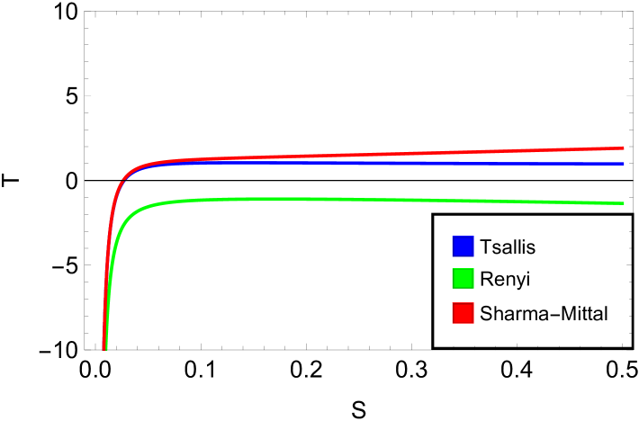
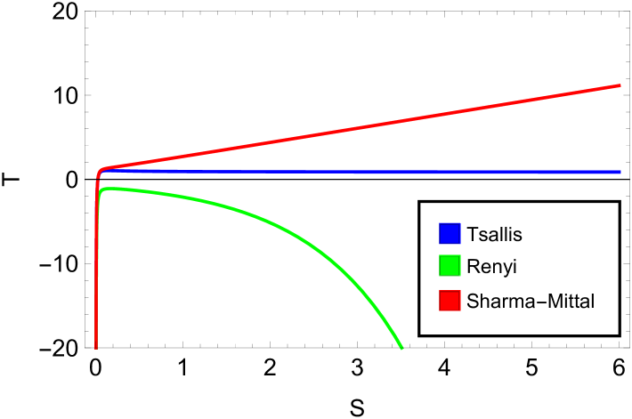
Figure 1: $T$ versus Tsallis, Rényi is and SM entropy $S$ for different values of cloud string $a$ (left panel) and $q$ (right panel) while other parameters are $\beta=1$, $\delta=4$, $R=2$, $\alpha=0.9$, and $P=1$, are held constant. Here, the trajectory of Tsallis, Rényi, and SM entropy are presented in blue, green, and red solid lines, respectively.

In this study, we explore the relationships between temperature and three different generalized entropies like the Tsallis, Rényi, and SM by considering a BH under the influence of a cloud of strings and electric charge. The analysis uses different values of the cloud of string parameter $a$ and charge $q$, while other parameters, including $\beta=1$, $\delta=4$, $R=2$, $\alpha=0.9$, and $P=1$, are held constant. Fig. 1 (left panel) depicts the relationship between temperature $T$ and Tsallis, Rényi, and SM entropies for different values of $a$. The Tsallis (blue curve) and SM (red curve) entropies show positive behavior, which indicates the physical behavior of BH, while Rényi (green curve) shows negative behavior, which demonstrates that Rényi entropy shows the non-physical behavior of BH. As the entropy increases, the temperature of SM (red curve) rises, and the graph becomes more positive. It suggests that higher entropy values correspond to higher temperatures, reinforcing the physical interpretation of the BH. Temperature initially shows negative behavior for lower entropy values; as the value of entropy increases, the temperature eventually starts increasing. Tsallis and SM become positive, but Rényi (green curve) entropy remains negative, indicating that the BH exhibits non-physical behavior. We conclude that SM (red curve) shows more physical behavior than Tsallis (blue curve) entropy, and Rényi (red curve) entropy shows non-physical behavior for different values of $a$. In Fig. 1 (right panel), we show a graph that compares Temperature with Tsallis, Rényi, and SM entropies for different values of $q$. The Tsallis (blue curve) and SM (red curve) entropies show positive values, indicating that the BH behaves physically across different values of $q$. On the other hand, the Rényi (green curve) entropy shows negative values, which suggests the BH behaves non-physically under these conditions. The graph helps us understand that the BH has different thermodynamic behavior depending on the type of entropy used. Tsallis (blue curve) and SM (red curve) entropies show that the BH stays in a physical state as temperature and entropy increase, making them useful for describing BH thermodynamics in situations involving a cloud of strings and electric charge. In contrast, Rényi (green curve) entropy behaves differently, showing non-physical behavior, particularly when considering the cloud of string and charge parameters. This difference may indicate limitations in applying Rényi entropy to BH systems in particular physical contexts, specifically when external fields like strings and charges are considered.

III.3 Specific Heat Capacity

In BH thermodynamics, the heat required to change a BH temperature is called thermal or heat capacity. Heat or thermal capacity is a key measurable physical property in BH thermodynamics. The stability of a BH can be determined by its sign, with a positive sign indicating stability and a negative sign indicating instability. There are two types of heat capacities: one that measures the specific heat when heat is added at a constant pressure $C_{p}$ and another that measures the specific heat when heat is added at constant volume $C_{v}$. The heat capacity $C_{p}$ rodrigues2022bardeen ; ruppeiner2014thermodynamic ; davies1978thermodynamics is determined by using the relation which is given in Eq. (26)

$$C_{p}=\frac{\partial S}{\partial T}\bigg{|}_{P}T.$$ (32)

By utilizing the Eqs. (14) and (23) into Eq. (32), we can compute the heat capacity $C_{p}$ for the Tsallis entropy case, which is given by

$$C_{p}(\mathrm{Tsallis}) = \bigg{[}3\beta S\left(I^{\frac{2}{3\beta}}+q^{2}\right)\left\{I^{\frac{2}{3\beta}}\left(-a+8\pi I^{\frac{2}{3\beta}}P+1\right)+2(a-1)q^{2}\right\}\bigg{]}\bigg{[}I^{\frac{4}{3\beta}}\bigg{\{}a$$ (33)

$$\times (3\beta-1)-3\beta+8\pi(2-3\beta)Pq^{2}+1\bigg{\}}-2(a-1)(3\beta+2)q^{4}-(a-1)I^{\frac{2}{3\beta}}$$

$$\times (3\beta+2)q^{2}-24\pi I^{2/\beta}(\beta-1)P\bigg{]}^{-1}.$$

Similarly, we obtained $C_{P}$ in the case of Rényi entropy by employing Eqs. (15) and (24) in Eq. (32) and it can be written as

$${C_{p}(\mathrm{Renyi})} = \bigg{[}3N\left(2^{2/3}N^{2/3}+\pi^{4/3}\alpha^{2/3}q^{2}\right)\left\{\sqrt[3]{\pi}(a-1)\alpha^{2/3}\left(N_{1}-N^{2/3}\right)+8\ 2^{2/3}N^{4/3}P\right\}\bigg{]}$$ (34)

$$\times \bigg{[}8\sqrt[3]{2}\alpha NP\left\{2e^{\alpha S}\left(N_{1}\sqrt[3]{N}+3e^{\alpha S}-6\right)-3N_{1}\sqrt[3]{N}+6\right\}-\sqrt[3]{\pi}(a-1)\alpha^{5/3}\bigg{\{}3$$

$$\times \left(\pi^{4/3}\alpha^{2/3}N^{2/3}q^{2}+2^{2/3}\sqrt[3]{N}+\pi^{2}\alpha^{2/3}q^{2}\right)+e^{\alpha S}\big{(}2\pi^{4/3}\alpha^{2/3}N^{2/3}q^{2}+2\pi^{2}\alpha^{2/3}N_{1}q^{2}$$

$$- 4\ 2^{2/3}\sqrt[3]{N}\big{)}+2^{2/3}\sqrt[3]{N}e^{2\alpha S}\bigg{\}}\bigg{]}^{-1}.$$

Furthermore, in case of SM entropy, $C_{p}$ is computed by employing the Eqs. (16) and (25) in Eq. (32) which takes the following form

$$C_{p}{(\mathrm{SM)}} = \bigg{[}3\delta^{2/3}X_{1}X\left(\pi^{4/3}q^{2}+\frac{2^{2/3}X^{2/3}}{\delta^{2/3}}\right)\bigg{\{}\sqrt[3]{\pi}(a-1)\delta^{2/3}\left(X_{2}-X^{2/3}\right)+8\ 2^{2/3}P$$ (35)

$$\times X^{4/3}\bigg{\}}\bigg{]}\bigg{[}\sqrt[3]{\pi}(a-1)\delta^{2/3}\bigg{\{}3RX\bigg{(}2^{2/3}X^{4/3}-\pi^{4/3}\delta^{2/3}q^{2}\left(X^{2/3}+X_{2}\right)\bigg{)}-\pi^{4/3}\delta^{5/3}q^{2}$$

$$\times \left(X^{2/3}+X_{2}\right)\left(2X_{1}^{\delta/R}+3\right)-2^{2/3}\delta\sqrt[3]{X}\left(-4X_{1}^{\delta/R}+X_{1}^{\frac{2\delta}{R}}+3\right)\bigg{\}}-8\sqrt[3]{2}PX\bigg{\{}\delta$$

$$\times \left(-X_{2}\right)\sqrt[3]{X}\left(2X_{1}^{\delta/R}-3\right)+3RX\left(2X_{1}^{\delta/R}+X_{2}\sqrt[3]{X}-2\right)-6\delta X^{2}\bigg{\}}\bigg{]}^{-1}.$$

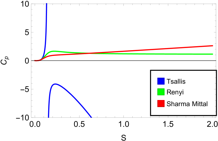
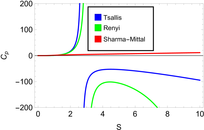
Figure 2: $C_{p}$ versus Tsallis, Rényi, SM entropy $S$ for different values of cloud string $a$ (left panel) and $q$ (right panel) and other parameters are $\beta=1$, $\delta=4$, $R=2$, $\alpha=0.9$, and $P=1$, are held constant. Here, the trajectory of Tsallis, Rényi, and SM entropy are presented in blue, green, and red solid lines, respectively.

Fig. 2 shows the BH-specific heat analysis using the Tsallis (blue curve), Rényi (green curve), and SM (red curve) entropy frameworks for different values of cloud string a (left panel) and q (right panel) and other parameter include $\beta=1$, $\delta=4$, $R=2$, $\alpha=0.9$, and $P=1$, are held constant. The plots show how specific heat changes with the size of the BH and its effects on stability and phase transitions. The heat capacity is an important measure of the BH thermodynamic stability. A positive heat capacity means the BH is stable and can reach thermal equilibrium with its surroundings. In contrast, a negative heat capacity means that the BH is unstable and cannot reach equilibrium. When the heat capacity is zero, it indicates a critical phase transition. In the left panel of Fig. 2, we examine how Tsallis (blue curve), Rényi (green curve), and SM (red curve) entropies affect the BH thermal stability for different values of $a$. The graph shows that the SM (red curve) and Rényi (green curve) entropy have positive heat capacities, indicating stable BH. The Tsallis (blue curve) entropy also starts with positive heat capacity, showing stability, but as $S$ increases, it undergoes a phase transition and becomes negative, indicating a change to unstable behavior. We also see that SM (red curve) is shown to be more stable than Rényi(green entropy) entropy. In the right panel of Fig. 2, we plot the specific heat capacity for the entropies of Tsallis (blue curve), Rényi (green curve), and SM (red curve) at different values of $q$. Initially, the Tsallis (blue curve) and Rényi (green curve) entropies are positive, indicating stability. After that, as $S$ increases, they undergo a phase transition at zero entropy and become negative. In contrast, the SM (red curve) entropy remains positive, reflecting stable behavior. This analysis shows that the BH behaves differently depending on which entropy framework is used. SM (red curve) entropy appears to show greater stability than both Tsallis (blue curve) and Rényi (green curve) entropies, especially when considering factors such as the cloud of strings $a$ and electric charge $q$. It suggests that SM entropy may be more suitable for describing BH thermodynamics under these conditions.

III.4 The HELMHOLTZ FREE ENERGY

Helmholtz free energy detailed in Refs. caneva2021helmholtz ; paul2024thermodynamics ; simovic2024euclidean serves as a tool to examine BHs global stability and is defined as

$$G=H_{M}-S\ T.$$ (36)

As we know in extended thermodynamics, BH mass can be interpreted as the enthalpy of the system instead of internal energy. By utilizing Eqs. (14), (20) and (23) in Eq. (36), then the Helmholtz free energy of Tsallis entropy can be obtained,

$$F_{\mathrm{Tsallis}} = -\frac{1}{6\beta}\bigg{[}I^{-\frac{2}{3\beta}-1}\left(I^{1/\beta}\right)^{\beta}\sqrt{I^{\frac{2}{3\beta}}+q^{2}}\left\{I^{\frac{2}{3\beta}}\left(-a+8\pi I^{\frac{2}{3\beta}}P+1\right)+2(a-1)q^{2}\right\}\bigg{]}$$ (37)

$$- \frac{1}{6}I^{-\frac{2}{3\beta}}\left(I^{\frac{2}{3\beta}}+q^{2}\right)^{3/2}\left(3a-8\pi I^{\frac{2}{3\beta}}P-3\right).$$

Similarly, by utilizing Eqs. (15), (21) and (24) in Eq. (36), then the Helmholtz free energy for Rényi entropy can be derived as

$$F_{\mathrm{Renyi}} = \frac{e^{\alpha S}\sqrt{\frac{2^{2/3}N^{2/3}}{\alpha^{2/3}}+\pi^{4/3}q^{2}}\log\left(e^{\alpha S}\right)\bigg{\{}\sqrt[3]{\pi}(a-1)\alpha^{2/3}\left(N^{2/3}-N_{1}\right)-8\ 2^{2/3}N^{4/3}P\bigg{\}}}{6\pi\alpha^{2/3}N^{5/3}}$$ (38)

$$+ \frac{\pi^{4/3}\alpha^{2/3}\left(\frac{2^{2/3}N^{2/3}}{\pi^{4/3}\alpha^{2/3}}+q^{2}\right)^{3/2}\left\{-3a+\frac{8\ 2^{2/3}N^{2/3}P}{\sqrt[3]{\pi}\alpha^{2/3}}+3\right\}}{6\ 2^{2/3}N^{2/3}}.$$

Now, by utilizing Eqs. (16), (22) and (25) in Eq. (36), then we obtained the Helmholtz free energy of SM entropy is given as

$$F_{\mathrm{SM}} = \frac{1}{6\pi RX^{5/3}}\bigg{[}\sqrt[3]{\delta}\sqrt{\pi^{4/3}q^{2}+\left(2X\delta^{-1}\right)^{2/3}}\left\{(\pi X+1)^{R/\delta}-1\right\}X_{1}^{\frac{\delta}{R}-1}\bigg{\{}\sqrt[3]{\pi}(a-1)\delta^{2/3}\big{(}X^{2/3}$$ (39)

$$- X_{2}\big{)}-8\ 2^{2/3}PX^{4/3}\bigg{\}}\bigg{]}+\frac{\pi^{4/3}\delta^{2/3}\left(q^{2}+\frac{2^{2/3}X^{2/3}}{\pi^{4/3}\delta^{2/3}}\right)^{3/2}\left\{-3a+\frac{8\ 2^{2/3}PX^{2/3}}{\sqrt[3]{\pi}\delta^{2/3}}+3\right\}}{6\ 2^{2/3}X^{2/3}}.$$

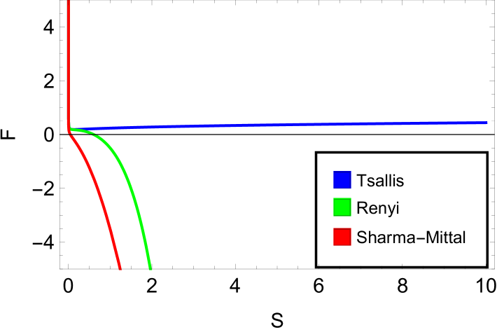
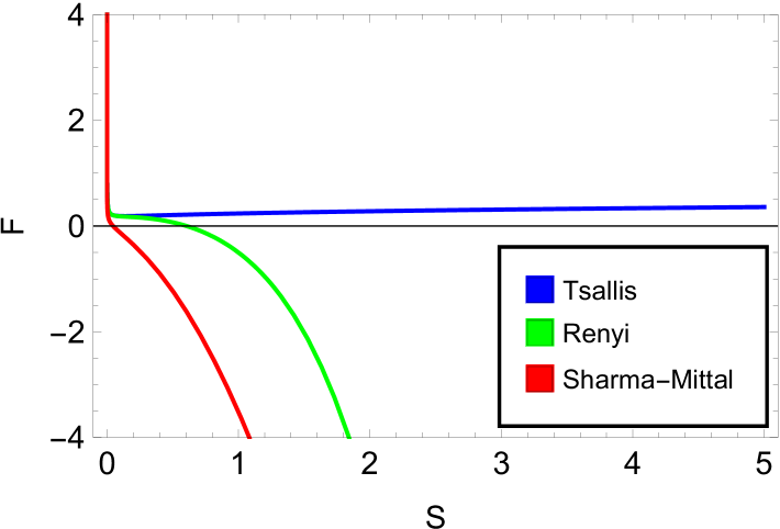
Figure 3: The Helmholtz free energy versus Tsallis, Rényi and SM entropy $S$ for different value of cloud string $a$ (left panel) and $q$ (right panel) while other parameters are $\beta=1$, $\delta=4$, $R=2$, $\alpha=0.9$, and $P=1$, are held constant. Here, the trajectory of Tsallis, Rényi, and SM entropy are presented in blue, green, and red solid lines, respectively.

In Fig. 3, we compare Helmholtz free energy for Tsallis (blue curve), Rényi (green curve), and SM (red curve) entropies to analyze the BH stability for different values of $a$ and $q$. Positive Helmholtz free energy indicates stability, negative values suggest instability, and zero marks a phase transition. In the left panel, the Tsallis entropy (blue curve) stays positive for varying $a$, showing stability. However, the Rényi (green curve) and SM (red curve) entropies start positive but turn negative as $S$ increases, indicating phase transitions and instability. Specifically, the Rényi entropy becomes negative at $S=0.8$, and the SM entropy transitions at $S=0.1$. In the right panel, for different $q$, the Tsallis entropy(blue curve) again remains positive, reflecting stable behavior. Meanwhile, both the Rényi(green curve) and SM(red curve) entropies begin positive, but Rényi entropy and SM entropies turn negative at $S=0.9$, $S=0.01$ respectively, and signify instability for the BH as entropy increases. This analysis shows that the BH behaves differently depending on which entropy framework is used. The graph shows that Tsallis entropy shows stability, while Rényi and SM entropies show instability for different values of $a$ and $q$. These results suggest that these entropy frameworks are useful for describing BH thermodynamics, particularly in the context of the cloud of strings and electric charge. However, Rényi and SM entropies behave differently, showing instability under certain conditions, like the cloud of strings $a$ and charge $q$. This suggests that Rényi and SM entropies may have limitations in describing BH systems in these specific physical contexts.

III.5 The GIBBS FREE ENERGY

The Gibbs free energy plays an important role in studying the BH global stability and phase transition. Detailed of the Gibbs free energy in Refs. ali2019thermodynamics ; kubizvnak2012p ; deng2018thermodynamics and is defined as

$$G=H_{M}-S\ T+PV.$$ (40)

To find the Gibbs free energy, we use Eqs. (14), (20), (23), (26) and (29) in Eq (40), then the Gibbs free energy of Tsallis entropy is given as,

$$G_{\mathrm{Tsallis}} = \frac{1}{6\beta}\pi^{-2\beta}I^{-1-\frac{2}{3\beta}}\sqrt{q^{2}+I^{\frac{2}{3\beta}}}(-\left((-1+a)q^{2}\left(2\pi^{2\beta}I+3\times 2^{\beta}S\beta\right)\right)-8P\pi^{\frac{4}{3\beta}}\left(\pi^{2\beta}\left(I-2^{1-\beta}S\beta\right)+I^{\frac{2}{3\beta}}\right)$$ (41)

$$\times \left((-1+a)\pi^{2\beta}\left(I-2^{\beta}\times(-3+3a-16P\pi q^{2})S\beta\right)\right))$$

Similarly, we use Eqs. (15), (21), (24), (27) and (30) in Eq (40), then the Gibbs free energy of Rényi entropy is given as,

$$G_{\mathrm{Renyi}} = \frac{1}{12N^{5/3}\pi\alpha^{2/3}}\sqrt{\pi^{4/3}q^{2}+\frac{2^{2/3}N^{2/3}}{\alpha^{2/3}}}(\left(N32N^{1/3}P\left(-2^{2/3}+2^{2/3}aS^{\alpha}+N^{1/3}\pi^{4/3}q^{2}\alpha^{2/3}\right)\right)-3x(-1+a)\pi^{1/3}$$ (42)

$$\times \left(2N^{2/3}+N_{1}\right)\alpha^{2/3}+2S^{\alpha}\left(-8\times 2^{2/3}N^{4/3}P+(-1+a)x^{2/3}\left(N^{2/3}-N_{1}\right)\alpha^{2/3}\right)\log(S^{\alpha}))$$

Now again similarly, by using Eqs. (16), (22), (25), (28) and (31) in Eq (40), then the Gibbs free energy of SM entropy is given as,

$$G_{\mathrm{SM}} = \frac{1}{12\pi RX^{5/3}\delta^{2/3}}\sqrt{\pi^{4/3}q^{2}+\frac{2^{2/3}X^{2/3}}{\delta^{2/3}}}(16PRX^{5/3}(2^{2/3}X^{2/3}\delta^{2/3})+2^{1/3}RX(8\cdot 2^{2/3}PX^{2/3}-3x(-1+a)\pi^{1/3}$$ (43)

$$\times \delta^{2/3})(2^{2/3}X^{2/3}+\pi^{4/3}q^{2}\delta^{2/3})-2X_{1}^{1-\frac{6}{R}}(-1+(1+\pi X)^{R/6})(8\times 2^{\frac{2}{3}}PX^{\frac{1}{3}}+(-1+a)\pi^{\frac{1}{3}}(-X^{\frac{2}{3}}+2^{\frac{1}{3}}\pi^{\frac{4}{3}}q^{2}\delta^{\frac{2}{3}}$$

$$\times )\delta^{\frac{2}{3}}\delta)$$

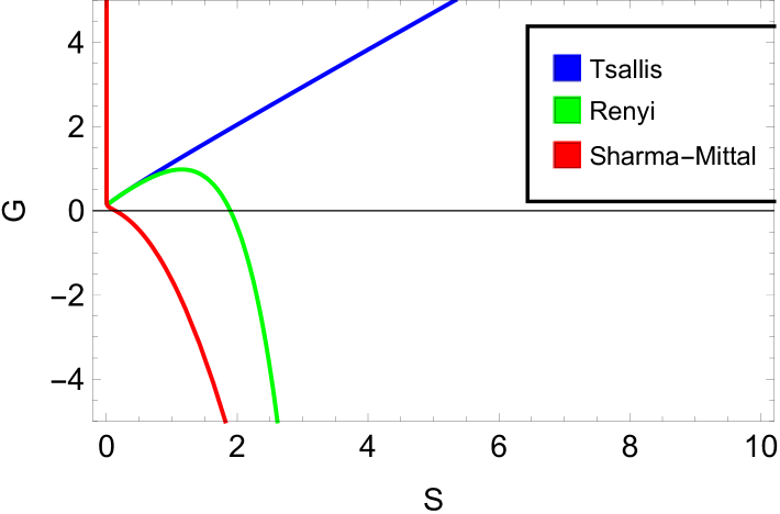
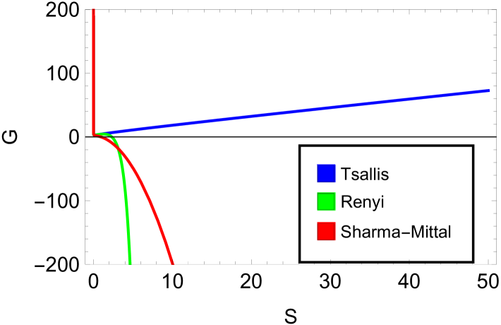
Figure 4: The Gibbs free energy versus Tsallis, Rényi and SM entropy $S$ for different value of cloud string $a$ (left panel) and $q$ (right panel) while other parameters are $\beta=1$, $\delta=4$, $R=2$, $\alpha=0.9$, and $P=1$, are held constant. Here, the trajectory of Tsallis, Rényi, and SM entropy are presented in blue, green, and red solid lines, respectively.

In Figure 4, we compare the Gibbs free energy for Tsallis (blue curve), Rényi (green curve), and SM (red curve) entropies to study BH stability for different values of $a$ and $q$. A positive Gibbs free energy indicates stability, a negative value suggests instability, and zero marks a phase transition. In the left panel, the Tsallis entropy (blue curve) remains positive for varying a, indicating stability. On the other hand, the Rényi entropy (green curve) starts positive but turns negative as entropy S increases, while the SM entropy (red curve) begins at zero and becomes negative, signaling phase transitions and instability. Specifically, the Rényi entropy becomes negative at $S=2.6$ and the SM entropy transitions at $S=0.3$. In the right panel, for different values of $q$, the Tsallis entropy (blue curve) again stays positive, reflecting stable behavior. In contrast, both the Rényi (green curve) and SM (red curve) entropies start at zero, with the Rényi entropy turning negative at $S=2.5$ and the SM entropy at $S=0.1$, indicating instability as entropy increases. This analysis reveals that the BH behavior depends on the entropy framework used. The Tsallis entropy consistently shows stability, while the Rényi and SM entropies exhibit instability under certain conditions for different values of $a$ and $q$. These findings suggest that these entropy frameworks are useful for describing BH thermodynamics, the Rényi and SM entropies may have limitations in describing BH systems under specific physical conditions, such as those involving the cloud of strings parameter $a$ and $q$.

IV Extensive exploration of Thermal Geometries

Geometric principles, reflected in thermodynamic geometry, have greatly enhanced our comprehension of BH thermodynamic structure. The curvature scalar is an invariant defined within this parameter space, providing deeper insights into phase transitions and the microscopic nature of BH. These concepts are proposed within the framework of thermal fluctuation theory, which has given rise to thermodynamic geometry. Usually, geothermodynamics is employed to study the interaction nature of the microstructures of the BHs. Now, we will examine the thermodynamic geometry associated with the Bardeen BH. To facilitate this investigation, we employ the geothermodynamics framework that enables the analysis of intricate connections between thermodynamic variables and the underlying geometric framework. Various methodologies will be explored in this analysis, such as the Weinhold, Ruppeiner, Quevedo-I, and Quevedo-II formalisms, each metric formalism possessing its advantages and limitations. Specifically, negative scalar curvatures indicate dominant attractive micro-interactions, while positive curvatures suggest repulsive interactions. A flat curvature signifies non-interacting systems, like an ideal gas, or systems where Interactions are perfectly balanced. Therefore, by selectively utilizing these diverse approaches, we aim to comprehensively address the geometric intricacies inherent in the Bardeen BH thermodynamics.

IV.1 Basic Formalisms of Geothermodynamics

To begin with, we delve into the Weinhold geometry, a method that offers a window to represent the thermal landscape visually. We have thoroughly examined the line element, determining the geometry as efficiently expressed in Ref. Jawad:2023jkb , and it is given as

$$g^{W}_{ik}=\partial_{i}\partial_{k}M(S,q),$$ (44)

and

$$ds^{2}_{W}=M_{SS}dS^{2}+M_{qq}dq^{2}+2M_{Sq}dSdq.$$ (45)

The two-dimensional metric for a Bardeen BH can be represented by the following matrix

$$g^{W}=\begin{bmatrix}M_{SS}&M_{Sq}\\ M_{qS}&M_{qq}\end{bmatrix}.$$ (46)

In our case, the Bardeen BH spacetime is $2$-dimensional, therefore the metric tensor elements take the given shape $g_{SS},~g_{Sq},~g_{qS}$ and $g_{qq}$ by using the mass function. Thereby, the components of Weinhold metrics are given below in the form of the mass function as

$$M_{SS}=\frac{\partial^{2}M(S,q)}{\partial S^{2}},M_{Sq}=\frac{\partial^{2}M(S,q)}{\partial S\partial q},$$ (47)

$$M_{qS}=\frac{\partial^{2}M(S,q)}{\partial q\partial S},M_{qq}=\frac{\partial^{2}M(S,q)}{\partial q^{2}}.$$ (48)

Now, we shift our focus to alternative geothermodynamic approaches that have yielded more effective physical outcomes. In the subsequent phase, we will examine the thermodynamic geometry of Bardeen BH is enveloped by string clouds that employ the Quevedo (I-II) metrics. The mathematical representation of the Quevedo metric is as follows Jawad:2023jkb

$$g=\bigg{(}E^{c}\frac{\partial\Phi}{\partial E^{c}}\bigg{)}\bigg{(}\eta_{ab}\delta^{bc}\frac{\partial^{2}\Phi}{\partial E^{c}\partial E^{d}}dE^{c}dE^{d}\bigg{)},$$ (49)

$$\frac{\partial\Phi}{\partial E^{c}}=\delta_{cb}l^{b}.$$ (50)

The thermodynamic potential has allowed us to incorporate a wider variety of variables in the thermodynamic framework, including extensive variables such as $E^{c}$ and intensive variables such as $I^{b}$. The Ruppeiner and the Weinhold’s geometric methods do not exhibit Legendre invariance. It indicates that the Ruppeiner, and the Weinhold metrics might yield conflicting results on occasion. To address these inconsistencies, the Quevedo (I-II) introduced a novel Legendre-invariant framework, which ensures that its characteristics remain unchanged under Legendre transformations. Within this framework, we encounter two distinct Legendre-invariant thermogeometric metrics, the Quevedo (I-II). The groundwork for these metrics was laid by Hermann and Mrugala mrugala1978geometrical , a foundation that the Quevedo (I-II) have further developed and applied. In the examination of thermodynamic systems, the utilization of this Legendre-invariant technique ensures consistency and compatibility.

$$ds^{2}=\begin{cases}\big{(}SM_{S}+QM_{q}\big{)}\big{(}-M_{SS}dS^{2}+M_{qq}dq^{2}\big{)}&\text{Quevedo Case I}\\ \big{(}-M_{SS}dS^{2}+M_{q}dq^{2}\big{)}\ SM_{S}&\text{Quevedo Case II}.\end{cases}$$ (51)

The formulation of the denominator for the curvature scalar in these metrics is constructed as outlined in Ref. Soroushfar:2019ihn

$$\text{denom }R(\text{Quevedo I}) =2M_{SS}^{2}M_{qq}^{2}\big{(}SM_{S}+qM_{q}\big{)}^{3},$$ (52)

$$\text{denom }R(\text{Quevedo II}) =2S^{3}M_{SS}^{2}M_{qq}^{2}M_{S}^{3}.$$

A briefed investigation of the Eqs. (41) and (42) demonstrates that the curvature scalar computed from the Quevedo formalism fails to offer significant physical information regarding the system.

IV.2 Tasallis Correction

This subsection incorporates the Tasallis entropy correction in the geothermodynamic framework to discuss the microscopic interaction between the particles of the Bardeen BH surrounded by clusters of strings. Thereby, we computed the second-order derivatives of BH’s mass, which yield

$$M_{SS} = \frac{1}{18S^{2}\sqrt{q^{2}+I^{\frac{0.66}{\beta}}\beta^{2}}}I^{\frac{-0.66}{\beta}}\bigg{[}-24P\pi I^{\frac{2}{\beta}}(-1+\beta)-2(-1+a)q^{4}(2+3\beta)$$ (53)

$$- (-1+a)q^{2}I^{\frac{0.66}{\beta}}(2+3\beta)+I^{\frac{1.33}{\beta}}\big{\{}1+8P\pi q^{2}\big{(}2-3\beta\big{)}-3\beta+a(-1+3\beta)\big{\}}\bigg{]},$$

$$M_{Sq} = \frac{1}{6S\sqrt{q^{2}+I^{\frac{0.66}{\beta}}\beta}}I^{\frac{-0.66}{\beta}}\bigg{[}6(-1+a)q^{3}+qI^{\frac{0.66}{\beta}}\bigg{\{}-3+3a+8P\pi I^{\frac{0.66}{\beta}}\bigg{\}}\bigg{]},$$ (54)

$$M_{qS} = \frac{1}{6S\sqrt{q^{2}+I^{\frac{0.66}{\beta}}\beta}}I^{\frac{-0.66}{\beta}}\bigg{[}6(-1+a)q^{3}+qI^{\frac{0.66}{\beta}}\bigg{\{}-3+3a+8P\pi I^{\frac{0.66}{\beta}}\bigg{\}}\bigg{]},$$ (55)

$$M_{qq} = \frac{1}{2\sqrt{q^{2}+I^{\frac{0.66}{\beta}}}}\bigg{\{}I^{\frac{-0.66}{\beta}}I^{\frac{0.66}{\beta}}\bigg{\}}\bigg{\{}3-3a+8P\pi I^{\frac{0.66}{\beta}}\bigg{\}}.$$ (56)

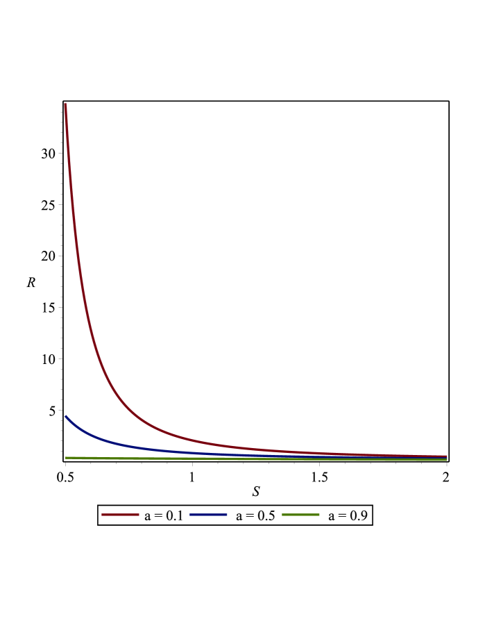
Figure 5: Ruppeiner curvature versus Tsallis entropy $S$ by inserting $q=0.5$, $a=0.1$ (red trajectory), $a=0.5$ (blue trajectory) and $a=0.9$ (green trajectory).

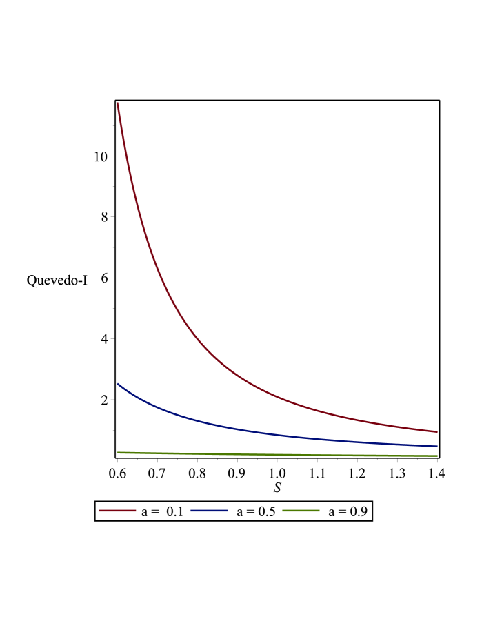
Figure 6: Quevedo-I versus Tsallis entropy $S$ by utilizing $q=0.5$, $a=0.1$ (red trajectory), $a=0.5$ (blue trajectory) and $a=0.9$ (green trajectory).

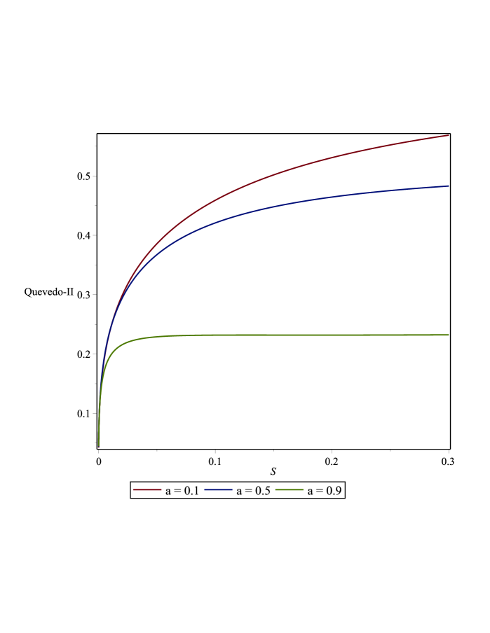
Figure 7: Quevedo-II versus Tsallis entropy $S$ by substituting $q=0.5$, $a=0.1$ (red trajectory), $a=0.5$ (blue trajectory) and $a=0.9$ (green trajectory).

In Fig. 6, we plot a graph between the Ruppeiner curvature and Tsallis entropy by inserting $q=0.5$, $a=0.1$ (red trajectory), $a=0.5$ (blue trajectory), and $a=0.9$ (green trajectory), which shows positive behavior, indicating that microscopic structure experiences repulsive interaction. This shows that components repel each other, leading to a more dispersed configuration. The system shows stability as the repulsive force prevents collapse and condensation. In Figs. 6 and 7, we plot a graph between the Quevedo (I-II), and Tsallis entropy by putting $q=0.5$, $a=0.1$ (red trajectory), $a=0.5$ (blue trajectory), and $a=0.9$ (green trajectory), and the graph shows positive behavior. The positive behavior shows stability, and the system exhibits repulsive interactions among its microstructure. The positive Quevedo (I-II) curvature shows that the system components tend to repel each other, leading to a more expanded, dispersed configuration. The Quevedo-II metric formalism shows more stable behavior than the Quevedo-I metric formalism for different values of $a$. Let us mention here the reason why we study thermodynamic geometry formalisms for only Tsallis entropy. The thermodynamic curvature for the Ruppeiner, Quevedo (I-II) formalisms with Rényi and Sharma-Mittal (SM) entropies is complex, making analytical computations impossible. However, by setting q=0, we significantly simplify the analysis, as the thermodynamic curvature for Ruppeiner and Quevedo (I-II) in the case of Rényi and SM entropies becomes zero. This allows us to extract meaningful physical interpretations regarding BH stability and microscopic interactions without unnecessary computational complications. The chosen model, which is Tsallis entropy, effectively captures the influence of external parameters like a cloud of strings and charge while ensuring that the thermodynamic geometry analysis remains tractable and insightful.

Table 1: Summary of thermodynamic quantities by using the Tsallis, Rényi, and SM entropies for the Bardeen BH and also its comparison with the thermodynamic quantities of the Schwarzschild BH. Here, we present the thermodynamic quantities like temperature, Heat capacity, Gibbs free energy, and Helmholtz free energy by $T,~C,~G$ and $F$, respectively.

Quantity	Tsallis	Rényi	SM	Bardeen BH	Schwarzschild BH
$T$	Stable	Unstable	Stable	Stable	Unstable
$C$	Unstable	Unstable	Stable	Unstable	Unstable
$G$	Stable	Unstable	Unstable	Stable	Stable
$F$	Stable	Unstable	Unstable	Stable	Unstable

V Conclusions

This study has presented the effects of generalized entropy on the Bardeen BH surrounded by clusters of strings. To govern the behavior of the string cloud, we modified the action of NED by employing the action of Nambu-Goto. Through the examination of the Kretschmann scalar, we explored a metric that displays singularities related to its parameter $a$. We explored the thermal characteristics of this solution by treating the equation of mass of the BH $M$ as the foundational equation. We interpreted the BH mass as enthalpy by emphasizing thermodynamic pressure $P$ and entropy $S$ as crucial parameters. This approach allowed us to conduct a comprehensive thermodynamic analysis by calculating the first-order differentiation of enthalpy, which is associated with thermodynamic potentials. Following standard practices in BH thermodynamics, we evaluated the stability of the solution by examining the thermodynamic quantities, particularly the heat capacity $C_{p}$, under the effect of the Tsallis, Rényi, and SM entropies. We assessed the solution stability across two different regions, which was distinguished by an unstable interval. The occurrence of an inconsistency indicated a phase transition of first order. We plotted a graph between the heat capacity $C_{p}$ and the Tsallis, Rényi, and SM entropies for different values of $a$ and $q$. We found that graphs show stable and unstable behavior of the BH. We provided a comprehensive analysis of the different models of entropy. We also find the Gibbs free energy of the Tsallis, Rényi, and SM entropies for different values of $a$. We find that the Tsallis entropy shows stable behavior, and the Rényi and SM entropies show unstable behavior.

Furthermore, we employed various thermodynamic geometric formalisms to comprehend the microscopic structure of the BH. Therefore, we investigated the Ruppeiner curvature, Quevedo (I-II), versus the Tsallis entropy for different values of $a$, and these graphs show that positive behavior indicates that microscopic structures experience repulsive interaction. This shows that components repel each other, leading to a more dispersed configuration. The positive Quevedo (I-II) curvature shows that the system components tend to repel each other, leading to a more expanded and dispersed configuration. The Quevedo-II shows more stable behavior than the Quevedo-I for different values of $a$. Furthermore, we observed that the curvature scalar of Ruppeiner, Quevedo (I-II) in terms of Rényi and SM entropies became zero, which further emphasizes that by employing Tsallis entropy, one can get better results as compared to the Rényi and SM entropies. Also, our results are more effective as we have comprehensively investigated and graphically presented the impact of various entropies. Furthermore, the Tsallis entropy might be quite helpful as it offers more valuable insights regarding the thermal stability of the BH, and it would be quite interesting to observe the thermodynamic behavior of BHs through the window of the Tsallis entropy.

References

- (1) G. W. Gibbons and S. W. Hawking, Phys. Rev. D 15, 2738-2751 (1977).
- (2) G. W. Gibbons, R. Kallosh and B. Kol, Phys. Rev. Lett. 77, 4992-4995 (1996).
- (3) S. W. Hawking, Commun. Math. Phys. 43, 199-220 (1975).
- (4) J. D. Bekenstein, Phys. Rev. D 7, 2333-2346 (1973).
- (5) C. Tsallis, J. Statist. Phys. 52, 479-487 (1988).
- (6) S. D. Odintsov and T. Paul, Phys. Dark Univ. 39, 101159 (2023).
- (7) J. D. Barrow, Phys. Lett. B 808, 135643 (2020).
- (8) B. Das, S. Moretti, S. Munir, and P. Poulose, Eur. Phys. J. C 81, 1 (2021).
- (9) G. Calcagni and L. Modesto, Phys. Lett. B 773, 596 (2017).
- (10) C. Rovelli, Phys. Rev. Lett. 77, 3288 (1996).
- (11) J. F. Barbero G and D. Pranzetti, Springer, 4085–4112 (2024).
- (12) A. Sayahian Jahromi, S. A. Moosavi, H. Moradpour, J. P. Morais Graça, I. P. Lobo, I. G. Salako and A. Jawad, Phys. Lett. B 780, 21-24 (2018).
- (13) G. Kaniadakis, Phys. Rev. E 72, 036108 (2005).
- (14) A. Majhi, Phys. Lett. B 775, 32-36 (2017).
- (15) Y. Liu, EPL 138, no.3, 39001 (2022).
- (16) A. Mandal, S. Samanta and B. R. Majhi, Phys. Rev. D 94, no.6, 064069 (2016).
- (17) A. Chamblin, R. Emparan, C. V. Johnson and R. C. Myers, Phys. Rev. D 60, 064018 (1999).
- (18) A. Chamblin, R. Emparan, C. V. Johnson and R. C. Myers, Phys. Rev. D 60, 104026 (1999).
- (19) S. H. Hendi and M. H. Vahidinia, Phys. Rev. D 88, no.8, 084045 (2013).
- (20) H. Yazdikarimi, A. Sheykhi and Z. Dayyani, Phys. Rev. D 99, no.12, 124017 (2019).
- (21) X. Y. Guo, H. F. Li, L. C. Zhang and R. Zhao, Phys. Rev. D 100, no.6, 064036 (2019).
- (22) M. Appels, R. Gregory and D. Kubiznak, Phys. Rev. Lett. 117, no.13, 131303 (2016).
- (23) M. Appels, R. Gregory and D. Kubiznak, JHEP 05, 116 (2017).
- (24) S. Gunasekaran, R. B. Mann and D. Kubiznak, JHEP 11, 110 (2012).
- (25) G. M. Deng, J. Fan, X. Li and Y. C. Huang, Int. J. Mod. Phys. A 33, no.03, 1850022 (2018).
- (26) F. Weinhold, J. Chem. Phys. 63, no.6, 2479 (1975).
- (27) G. Ruppeiner, Phys. Rev. A 20, no.4, 1608 (1979).
- (28) G. Ruppeiner, Rev. Mod. Phys. 67, 605-659 (1995).
- (29) H. Quevedo, J. Math. Phys. 48, 013506 (2007).
- (30) A. Al- Badawi, A. jawad, The Europ. Phys. Jour. C, 84, 115 (2024).
- (31) S. H. Hendi, S. Panahiyan, B. Eslam Panah and M. Momennia, Eur. Phys. J. C 75, no.10, 507 (2015).
- (32) S. H. Hendi, A. Sheykhi, S. Panahiyan and B. Eslam Panah, Phys. Rev. D 92, no.6, 064028 (2015).
- (33) S. Soroushfar and S. Upadhyay, Phys. Lett. B 804, 135360 (2020).
- (34) M. Chabab, H. El Moumni, S. Iraoui and K. Masmar, Eur. Phys. J. C 79, no.4, 342 (2019).
- (35) G. Ruppeiner, Phys. Rev. D 78, 024016 (2008).
- (36) A. Sahay, T. Sarkar and G. Sengupta, JHEP 07, 082 (2010).
- (37) A. Lala and D. Roychowdhury, Phys. Rev. D 86, 084027 (2012).
- (38) G. Q. Li and J. X. Mo, Phys. Rev. D 93, no.12, 124021 (2016).
- (39) A. Sahay, Phys. Rev. D 95, no.6, 064002 (2017).
- (40) M. Kord Zangeneh, A. Dehyadegari, A. Sheykhi and R. B. Mann, Phys. Rev. D 97, no.8, 084054 (2018).
- (41) S. Soroushfar, R. Saffari and S. Upadhyay, Gen. Rel. Grav. 51, no.10, 130 (2019).
- (42) K. Bhattacharya and B. R. Majhi, Phys. Lett. B 802, 135224 (2020).
- (43) A. N. Kumara, C. L. A. Rizwan, D. Vaid and K. M. Ajith, [arXiv:1906.11550 [gr-qc]].
- (44) A. A. A. Filho, K. Jusufi, B. Cuadros-Melgar and G. Leon, Phys. Dark Univ. 44, 101500 (2024).
- (45) S. Nojiri, S. D. Odintsov and V. Faraoni, Phys. Rev. D 105, no.4, 044042 (2022).
- (46) S. Nojiri, S. D. Odintsov and T. Paul, Phys. Lett. B 831, 137189 (2022).
- (47) S. Nojiri, S. D. Odintsov and V. Faraoni, Int. J. Geom. Meth. Mod. Phys. 19, no.13, 2250210 (2022).
- (48) E. Elizalde, S. Nojiri and S. D. Odintsov, Universe 11, no.2, 60 (2025).
- (49) S. D. Odintsov, S. D’Onofrio and T. Paul, Phys. Dark Univ. 42, 101277 (2023).
- (50) S. Nojiri, S. D. Odintsov and T. Paul, Universe 10, no.9, 352 (2024).
- (51) N. Drepanou, A. Lymperis, E. N. Saridakis and K. Yesmakhanova, Eur. Phys. J. C 82, no.5, 449 (2022). ++[arXiv:2109.09181 [gr-qc]].
- (52) M. E. Rodrigues and H. A. Vieira, Phys. Rev. D 106, no.8, 084015 (2022).
- (53) S. Hyun and C. H. Nam, Eur. Phys. J. C 79, no.9, 737 (2019).
- (54) A. Bakopoulos, N. Chatzifotis and T. Karakasis, Phys. Rev. D 110, no.10, 10 (2024) doi:10.1103/PhysRevD.110.L101502 [arXiv:2404.07522 [hep-th]].
- (55) J. D. Bekenstein, Phys. Rev. D 23, 287 (1981).
- (56) J. M. Bardeen, B. Carter and S. W. Hawking, Commun. Math. Phys. 31, 161-170 (1973).
- (57) R. M. Wald, Living Rev. Rel. 4, 6 (2001).
- (58) M. E. Rodrigues, M. V. de S. Silva and H. A. Vieira, Phys. Rev. D 105, no.8, 084043 (2022).
- (59) G. Ruppeiner, Springer Proc. Phys. 153, 179 (2014).
- (60) P. C. W. Davies, Phys. Rept. 41, 1313 (1978).
- (61) K. L. Caneva, Helmholtz, MIT Press, (2021).
- (62) P. Paul, S. I. Kruglov, Indian J. Phys. 98, 1201-1210 (2024).
- (63) F. Simovic, I. Soranidis, Phys. Rev. D. 109, 044029 (2024).
- (64) M. S. Ali and S. G. Ghosh, Phys. Rev. D 99, no.2, 024015 (2019).
- (65) D. Kubizňák, R. B. Mann, JHEP 1207 , 033 (2012).
- (66) G. M. Deng, J. Fan, X. Li and Y. C. Huang, Int. J. Mod. Phys. A 33, 1850022 (2018).
- (67) A. Jawad, M. Yasir and H. Raza, Eur. Phys. J. C 83, no.9, 882 (2023).
- (68) R. Mrugała, Repor. on. Math. Phys 14, 419 (1978).