Stochastic Thermodynamics of Non-reciprocally Interacting Particles and Fields

Abstract

Nonreciprocal interactions that violate Newton’s law ’actio=reactio’ are ubiquitous in nature and are currently intensively investigated in active matter, chemical reaction networks, population dynamics, and many other fields. An outstanding challenge is the thermodynamically consistent formulation of the underlying stochastic dynamics that obeys local detailed balance and allows for a rigorous analysis of the stochastic thermodynamics of non-reciprocally interacting particles. Here, we present such a framework for a broad class of active systems and derive by systematic coarse-graining exact expressions for the macroscopic entropy production. Four independent contributions to the thermodynamic dissipation can be identified, among which the energy flux sustaining vorticity currents manifests the presence of non-reciprocal interactions. Then, Onsager’s non-reciprocal relations, the fluctuation-response relation, the fluctuation relation and the thermodynamic uncertainty relations for non-reciprocal systems are derived. Finally, we demonstrate that our general framework is applicable to a plethora of active matter systems and chemical reaction networks and opens new paths to understand the stochastic thermodynamics of non-reciprocally interacting many-body systems.

1 Introduction

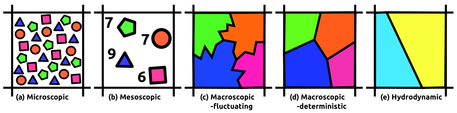
Figure 1: Scheme of various levels of coarse-graining considered in this paper, microscopic, mesoscopic, macroscopic-fluctuating, macroscopic-deterministic and hydrodynamic. (a) Microscopic particles are confined to the lattice site (denoted by the black $\#$). Four different types of particles are illustrated: triangle (blue), square (pink), pentagon (green) and, circle (orange). (b/c) The mesoscopic/macroscopic description is obtained for the fluctuating particle number/density. (d) The straight interface between the density fields represents the suppression of the fluctuation and convergence to the mean-field dynamical description. (e) Cyan and Yellow denote the relevant hydrodynamic order parameter that does not necessarily preserve the microscopic properties.

The discovery of fluctuation relations shed new light on the classical field of thermodynamics [1, 2, 3, 4, 5, 6, 7, 8, 9, 10, 11, 12, 13, 14, 15, 16, 17, 18, 19] and established the refined framework of stochastic thermodynamics (ST) [20, 21]. Stochastic thermodynamics accomplishes to define the first and second laws of thermodynamics for a single stochastic transition . This is achieved by defining the energy, work, heat and, entropy production for a stochastic transition, such that the thermodynamic quantities have probability distributions. Fluctuations vanish in the thermodynamic limit, hence the resulting stochastic thermodynamic quantities are peaked to the deterministic thermodynamic description. Recovering the traditional thermodynamic description in the thermodynamic limit. Stochastic thermodynamics applies to small systems with inherent stochastic fluctuations in the presence of an externally imposed driving of control parameters. The validity of this framework relies on a key constraint of time-scale separation which results in Markovian property for the transitions: states of the stochastic process comprise the slow degrees of freedom and the collective fast degrees of freedom form the thermal environment (bath). The Local Detailed Balance (LDB) condition establishes the equivalence between the forward and backward transition rates and the thermodynamic transition cost supported by the environment [23, 24] and ensures thermodynamic consistency for all transitions.

Newton’s third law of motion states that for every action force, there is equal and opposite reaction force. Multiple real-world counter-examples to Newton’s third law of motion exist. The systems violating Newton’s third law of motion are called non-reciprocal [25]. In particular, a multitude of biological systems are frontier to study and understand the implications of the violation of Newton’s third law of motion. For instance, toy models for ecological systems [26, 27, 28, 29, 30, 31, 32, 33, 34, 35, 36], stochastic systems [37, 38, 39], neural networks [40, 41, 42, 43, 44, 45, 46], a mixture of non-reciprocal particles [47], birds with vision cones [48], solids with odd elasticity [49], particles breaking action-reaction symmetry [50, 51], chiral active particles [52, 53], non-reciprocal flocking models [54, 55], non-reciprocal frustration [56], systems described by non-reciprocal Cahn-Hillard equations [57, 58, 59, 60, 61, 62, 63]. Recent developments in understanding the microscopic dynamics of non-reciprocal systems have revealed more sophisticated behaviors and phases that are otherwise absent in reciprocal systems. For example, travelling waves, oscillations, spiral waves, and effervescence [54, 55, 57, 58, 59, 60, 61, 62, 63]. The non-reciprocal phases have been understood by delineating the underlying topological properties [54].

Active matter and non-reciprocal systems are conventionally analyzed with the hydrodynamic description [64, 65], which successfully recovers the phases observed for the microscopic dynamics [55]. Deriving hydrodynamic equations of motion requires identifying the relevant degrees of freedom termed order parameter with the help of symmetry arguments: a top-down approach [64, 65]. Subsequently, one can incorporate the order parameter fluctuations by using more sophisticated exact coarse-graining techniques [66, 67]. This procedure is usually effective and reliable in understanding the system dynamics, phases, and phase transitions.

However, for microscopic systems, the hydrodynamic description fails quantitatively and qualitatively in the small particle number regime. For example, the onset of the phase transition predicted by the hydrodynamic description is different from that predicted by the microscopic description [68]. Moreover, it fails to predict the order of the phase transition which is usually addressed by introducing ad-hoc noise corrections [68]. The hydrodynamic description also fails to adequately describe and understand the thermodynamic implications at the macro/meso-scale because of coarse-graining. The effective hydrodynamic description does not resolve the microscopic dissipation at the hydrodynamic scale. In particular, the microscopic states with different thermodynamic properties are coarse-grained to a single-order parameter. In addition, the mapping between the microscopic and macroscopic/mesoscopic control parameters is less transparent. We aim to construct the macrostate dynamics using a bottom-up approach. We want to implement the coarse-graining procedure only up to an order in which the microscopic dissipation is both qualitatively and quantitatively preserved, and therefore avoid a subsequent coarse-graining to obtain an effective description in terms of relevant order parameters.

The coarse-graining scheme is shown in fig. 1. Microscopic particles with different dynamic and thermodynamic microscopic properties exist. Lumping together microstates with identical thermodynamic and physical properties forms a mesostate: the particle number. The macroscopic limit corresponds to taking the limit of a large number of particles per site. It defines the scaling from the intensive density order parameter to the extensive particle number. The densities are fluctuating stochastic fields, denoted by the rough edges. The thermodynamic limit suppresses the macroscopic fluctuations that lead to the reaction-diffusion dynamics for deterministic density fields. In comparison, the top-down construction of an effective hydrodynamic description fails to track the microscopic thermodynamic dissipation qualitatively and quantitatively.

Despite much progress in understanding the dynamics of active matter on different scales, its implications for the thermodynamics of non-reciprocal systems remain elusive. For reciprocal active matter systems the stochastic thermodynamics has been formulated for active Brownian particles [69, 70, 71] and for flocking models [72] and fluctuation relations have been derived [73, 74]. To quantify thermodynamic irreversibility, an information-theoretic measure has been utilized, as for instance for the Active Ising model [75] and the non-reciprocal Cahn-Hillard equation [76, 77, 78], which has been proven to be a good statistical measure to compute lower bounds for the thermodynamic entropy production [79, 80, 81, 82, 83, 84, 85]. However, the information-theoretic definition of irreversibility does not necessarily coincide with the thermodynamic entropy production [79, 80, 81, 82, 83, 84, 85]. The information theoretic irreversibility measure can be defined without the state transitions satisfying local detailed balance (LDB), thus lacking thermodynamic consistency [75, 76, 77].

We therefore combine in this paper the three main motifs mentioned so far: Stochastic Thermodynamics and Coarse-graining for the Nonreciprocal Interacting Particles. We aim to formulate a microscopic Markov jump process description for the interacting non-reciprocal particles, which enables us to define their dynamics and thermodynamics in a thermodynamically consistent way. Subsequently, we aim to implement a coarse-grained mesoscopic/macroscopic description that preserves the microscopic thermodynamic dissipation. We ensure this by properly identifying the LDB condition on the mesoscale/macroscale. We obtain the thermodynamically consistent dynamics for the time evolution of the mesostate/macrostate. Importantly, this ensures the thermodynamics for the non-reciprocal systems is defined at the mesoscale/macroscale. This allows us to establish the connection between the microscopic and macroscopic/mesoscopic control parameters, which allows a qualitative and quantitative equivalence between the dynamics and thermodynamic physical quantities. Importantly, this extends the applicability of Stochastic Thermodynamics to coarse-grained many-body descriptions.

We define the class of thermodynamically consistent lattice gas models for non-reciprocally interacting microscopic particles coupled to an external driving reservoir [1, 13, 20]. LDB for the microscopic system ensures the thermodynamic consistency of these models. This allows us to define the microscopic EPR for the externally driven non-reciprocal particles using the Markov Jump Process (MJP) and its dynamics governed by the Master equation [1, 13, 20]. Further, we define the coarse-grained state description (mesoscopic/macroscopic) by lumping microstates with identical dynamical and thermodynamical properties [86]. The mesoscopic/macroscopic scale is defined for the particle number/density as a coarse-grained state. The coarse-grained description is chosen flexibly depending on the system-specific requirement. We employ the Doi-Peliti exact coarse-graining method that preserves microscopic discreetness at the coarse-grained description [86].

Next, we formulate the transitions between the coarse-grained state using the LDB in a thermodynamically consistent way. This enables us to quantify and decompose the coarse-grained state dissipation using ST for any non-reciprocal system. In addition, the dynamic and thermodynamic equivalence of the microscopic and coarse-grained systems is ensured. The fluctuating dynamics of the coarse-grained states generalize the Macroscopic Fluctuating Theory (MFT) for the non-reciprocal systems [87]. We obtain the non-quadratic dissipation function that plays an important role in the exact quantification of the EPR (particularly for the far-from-equilibrium systems [88]. We decompose the EPR into its linearly independent contributions, namely orthogonal decomposition. It consists of four contributions, relaxation of the reciprocal interaction energy functional, non-reciprocal interaction, coupling to the external reservoir, and external driving work.

Finally, we demonstrate the non-reciprocal and non-equilibrium analogues of the reciprocal systems. For instance, the irreversible thermodynamics relations: the Onsager’s non-reciprocal relations, fluctuation-response relations, higher-order non-linear responses and, the stochastic thermodynamic relations: fluctuation relations, thermodynamic kinetic uncertainty relation. In the deterministic macroscopic limit, we recover the irreversible thermodynamics, the Arrhenius’s transition state theory (LDB) and reaction-diffusion systems (dynamics) for the interacting non-reciprocal density fields [89, 64, 65]. We elaborate on the application of our framework using a few prototypical models. Our framework extends the applicability of stochastic thermodynamics for non-reciprocal and externally driven systems across different observation scales.

2 Microscopic Description

2.1 Microscopic Boltzmann weight

We consider a multi-particle system that comprises several particle types and lives in discretized space, a regular lattice with lattice constant $l$, continuous time, and periodic boundary conditions. Physically, the lattice constant corresponds to using the microscopic diffusive length scale of the particles as a space measurement unit. The continuum limit $l\to 0$ leads to oversimplified coarse-grained description that does not account for the inherent diffusive length-scale of the system. Therefore, we consider $l=1$ in this paper unless we specify the continuum space limit $l\to 0$. The number of particles of type $i$ at the lattice site index $\#$ is denoted by $N_{i}^{\#}$. The configuration of the lattice is denoted by $\{N\}$. The dimension of the $\{N\}$ is decided by the lattice size and the number of particle types. The volume of the d-dimensional lattice space is denoted by $\mathcal{V}$. The faster degrees of freedom forms the environment which supports the thermodynamic cost for all microstate changes of the system which consist of the slower degrees of freedom.

The microscopic interaction energy experienced by type $i$ particle due to the type $j$ particle is denoted by $v_{ij}$. $v_{ij}<0$ implies type $i$ particle are attracted towards type $j$ particles, $v_{ij}>0$ holds true for the repulsive interaction. Formulated analogously, $v_{ij}$ is the thermodynamic cost supported by the environment to place a type $i$ particle in the presence of a type $j$ particle. The violation of the actio=reactio symmetry implies $v_{ij}\neq v_{ji}$ microscopically. $v_{ij}=v_{ji}$ implies the particles are reciprocal and respect the actio=reactio symmetry. To differentiate and quantify the actio=reactio symmetry preserving and breaking terms, we define the reciprocal $v_{ij}^{r}=(v_{ij}+v_{ji})/2$ and non-reciprocal $v_{ij}^{nr}=(v_{ij}-v_{ji})/2$ interaction energy between the type $i$ and type $j$ particles. $v_{ij}^{r}$ and $v_{ij}^{nr}$ correspond to the actio=reactio symmetry preserving and breaking components respectively. Importantly, this fixes ‘the orthogonal reference gauge’ such that the symmetry $v_{ij}^{r}=v_{ji}^{r}$ and anti-symmetry $v_{ij}^{nr}=-v_{ji}^{nr}$ is satisfied by construction.

The reciprocal and non-reciprocal components of the microscopic Boltzmann weight $\epsilon_{i}^{\#}$ of the type $i$ particle at $\#$ are defined as $\epsilon_{i}^{r}$ and $f_{i}^{nr}$ respectively , such that $\epsilon_{i}^{\#}=\epsilon_{i}^{r}+f_{i}^{nr}$,

$$\begin{split}\epsilon_{i}^{r}=\beta\sum_{j\neq i}v_{ij}^{r}N_{j}^{\#}+\beta v_{ii}^{r}\left(N_{i}^{\#}-1\right),\hskip 14.22636ptf_{i}^{nr}=\beta\sum_{j}v_{ij}^{nr}N_{j}^{\#}.\end{split}$$ (1)

Here, $N_{i}^{\#}-1$ takes care of the self-interaction of the particle. $\beta$ is the inverse temperature. We fix the Boltzmann constant to unity throughout this paper. $\epsilon_{i}^{r}$ and $f_{i}^{nr}$ correspond to the actio = reactio symmetry preservation and violation terms, respectively. They quantify the total reciprocal and nonreciprocal interaction energy experienced by the type $i$ particle owing to all other particles. $\epsilon_{i}^{r}$ and $f_{i}^{nr}$ are locally defined properties of each particle.

We examine the possibility of representing the locally defined microscopic Boltzmann weight as a global property of the lattice, namely the total interaction energy $\varepsilon^{int}$. The condition for it turns out to be $v_{ij}=v_{ji}$, which is satisfied by $v_{ij}^{r}$ and violated by $v_{ij}^{nr}$. Hence, the reciprocal part of the microscopic Boltzmann weight is written as the microscopic interaction energy functional $\varepsilon^{int}$ of the lattice,

$$\begin{split}\varepsilon^{int}=\frac{1}{2}\beta\sum_{\#,\>i}v_{ii}^{r}N_{i}^{\#}\left(N_{i}^{\#}-1\right)+\beta\sum_{\#,\>i\neq j}v_{ij}^{r}N_{i}^{\#}N_{j}^{\#}.\end{split}$$ (2)

In the absence of non-reciprocity, i.e. $v_{ij}^{nr}=0,\forall i,j$, the system satisfies the Boltzmann distribution generated by $\varepsilon^{int}$. A detailed discussion on thermodynamics is subsequently included.

The eq. 2 is not necessarily the equilibrium interaction energy functional. Consider the decomposition, $v_{ij}=v_{ij}^{eq}+v_{ij}^{neq}$. Where $v_{ij}^{eq}$ is derived from the equilibrium energy functional of the form eq. 2 and $v_{ij}^{neq}$ is the remaining microscopic non-equilibrium interaction energy attributed to the violation of Newton’s third law of motion. This leads to $v_{ij}^{r}=v_{ij}^{eq}+(v_{ij}^{neq}+v_{ji}^{neq})/2$ and $v_{ij}^{nr}=(v_{ij}^{neq}-v_{ji}^{neq})/2$, hence, $v_{ij}^{r}$ and $v_{ij}^{nr}$ incorporates the symmetric and anti-symmetric parts respectively of the $v_{ij}^{neq}$. In conclusion, even though the microscopic physical interaction rules are governed by $v_{ij},v_{ji},v_{ij}^{eq},v_{ij}^{neq}$, the underlying geometric and thermodynamic structure is governed by $v_{ij}^{r},v_{ij}^{nr}$, and $|\varepsilon^{int}|\geq|\varepsilon^{eq}|$ gives a tighter bound on the conservative interaction energy functional.

Moreover, this analysis reveals that the decomposition of $v_{ij}$ and $v_{ji}$ (gauge fixing) is not necessarily unique, unless ‘the orthogonal reference gauge’ is imposed. Further, it will be shown that only ‘the orthogonal reference gauge’ leads to observation scale invariant decomposition of actio-reactio symmetry conserving and breaking terms. Consequently, it also gives the physically correct thermodynamic dissipation of the system. The decomposition of $\epsilon_{i}^{\#}$ into $\epsilon_{i}^{r}$ and $f_{i}^{nr}$ is equivalent to the Helmholtz-Hodge decomposition of $\epsilon_{i}^{\#}$ into a conservative gradient force $\epsilon_{i}^{r}$ derived from $\varepsilon^{int}$ and a divergence-free non-conservative force $f_{i}^{nr}$.

2.2 Dynamics

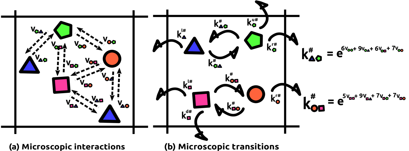
Figure 2: (a) The illustration for the microscopic interaction between the particle types denoted by $v_{ij}$ confined to the lattice site $\#$ such that $v_{ij}\neq v_{ji}$. (b) All possible transitions are denoted by a curved harpoon. The exact expression for two transition rates $k_{\gamma\gamma^{\prime}}$ in terms of $v_{ij}$ for the microscopic lattice configuration in fig. 1(a) are demonstrated.

A Single particle microstate transition rates

The particle can change its type or the lattice location, which is defined as the reactive and diffusive transition respectively. A reactive transition from type $\gamma^{\prime}$ to $\gamma$ in $\#$ is indicated by $\Delta_{\gamma\gamma^{\prime}}^{\#}$ resulting in $\{N\}\to\{N+\Delta_{\gamma\gamma^{\prime}}^{\#}\}$. Similarly, a diffusive transition of type $i$ particle from $\#$ in direction $\vec{\mathcal{D}}$ is indicated by $\Delta_{i}^{\vec{\mathcal{D}}\#}$ resulting in $\{N\}\to\{N+\Delta_{i}^{\vec{\mathcal{D}}\#}\}$. The transition rate of a reactive ($k_{\gamma^{\prime}\gamma}^{\#}$) and diffusive ($k_{i}^{\vec{\mathcal{D}}\#}$) jump are constructed using $\epsilon_{i}^{\#}$:

$$\begin{split}k_{\gamma^{\prime}\gamma}^{\#}=d_{\gamma^{\prime}\gamma}e^{\epsilon_{\gamma}^{\#}},\hskip 14.22636ptk_{i}^{\vec{\mathcal{D}}\#}=d_{i}^{\mathcal{D}}e^{\epsilon_{i}^{\#}}.\end{split}$$ (3)

The LDB for the forward and backward microscopic transitions read:

$$\begin{split}\frac{k_{\gamma\gamma^{\prime}}^{\#}}{k_{\gamma^{\prime}\gamma}^{\#}}=e^{\epsilon_{\gamma^{\prime}}^{\#}-\epsilon_{\gamma}^{\#}+f_{\gamma\gamma^{\prime}}^{ch}},\hskip 14.22636pt\frac{k_{i}^{\vec{\mathcal{D}}\#}}{k_{{i}}^{(\vec{\mathcal{D}}\#)^{-1}}}=e^{\epsilon_{i}^{\#}-\epsilon_{i}^{\vec{\mathcal{D}}\#}+\vec{\mathcal{D}}\cdot\vec{f}_{i}^{sp}}.\end{split}$$ (4)

The environment supports the thermodynamic cost for the change in the microscopic Boltzmann weight. We have modified eq. 4 by introducing a non-conservative external driving force $f_{\gamma\gamma^{\prime}}^{ch}$ and $\vec{f}_{i}^{sp}$ that correspond to chemical and self-propulsion driving. The thermodynamic cost for such an external driving is supported by an externally coupled reservoir of the enzymatic particles (for the reactive transition) or colloidal particles (for the diffusive transitions) respectively. We use shorthand notations $\Delta_{\gamma\gamma^{\prime}}^{\#}(*)=(*)_{\gamma^{\prime}}^{\#}-(*)_{\gamma}^{\#}$ and $\Delta_{i}^{\vec{\mathcal{D}}\#}(*)=(*)_{i}^{\#}-(*)_{i}^{\vec{\mathcal{D}}\#}$ for the change in $\epsilon_{i}^{\#},\epsilon_{i}^{r}$ and $f_{i}^{nr}$ due to a transition. We introduce a shorthand notation $\Delta$ for referring to a transition, applied as a diffusive or reactive transition depending on the context. The set of all reactive transitions is denoted by $\{\Delta_{\gamma\gamma^{\prime}}^{\#}\}$. The set of all diffusive transitions is denoted by $\{\Delta_{i}^{\vec{\mathcal{D}}\#}\}$. Four such possibilities for a two-dimensional square lattice exist: upward, downward, leftward, and rightward. The microscopic interactions and transitions are shown in fig. 2.

B Multi-particle microstate transition rates

Particles with identical type and lattice index have the same dynamic and thermodynamic properties. Hence, $k_{\gamma\gamma^{\prime}}^{\#}$ are lumped together to give multi-particle transition rates $k_{\gamma\gamma^{\prime}}^{\#}({\{N\}})=N_{\gamma^{\prime}}^{\#}k_{\gamma\gamma^{\prime}}^{\#}$ and ${k_{\gamma\gamma^{\prime}}^{\#}({\{N\}})}=N_{i}^{\#}k_{i}^{\vec{\mathcal{D}}\#}$. The LDB for the multi-particle transition rate for the reactive (${k_{\gamma\gamma^{\prime}}^{\#}({\{N\}})}$) and diffusive (${k_{{i}}^{\vec{\mathcal{D}}\#}(\{N\})}$) is:

$$\begin{split}\frac{k_{\gamma\gamma^{\prime}}^{\#}({\{N\}})}{k_{\gamma^{\prime}\gamma}^{\#}({\{N+\Delta_{\gamma\gamma^{\prime}}^{\#}\}})}&=e^{-\Delta_{\gamma\gamma^{\prime}}^{\#}s^{b}+\Delta_{\gamma\gamma^{\prime}}^{\#}\epsilon+f_{\gamma\gamma^{\prime}}^{ch}}.\\ \frac{k_{{i}}^{\vec{\mathcal{D}}\#}(\{N\})}{k_{i}^{(\vec{\mathcal{D}}\#)^{-1}}(\{N+\Delta_{i}^{\vec{\mathcal{D}}\#}\})}&=e^{-\Delta_{i}^{\vec{\mathcal{D}}\#}s^{b}+\Delta_{i}^{\vec{\mathcal{D}}\#}\epsilon+\vec{\mathcal{D}}\cdot\vec{f}_{i}^{sp}}.\end{split}$$ (5)

Where, $\Delta s^{b}$ incorporates the change in microscopic Boltzmann entropy defined as a global lattice property [91]:

$$\begin{split}s^{b}=\ln{\left[\frac{\left(\sum_{i,\#}N_{i}^{\#}\right)!}{\prod_{i,\#}N_{i}^{\#}!}\right]}.\end{split}$$ (6)

It quantifies the statistical degeneracy of the microstate and is a system property defined for the lattice. Importantly, $\Delta_{\gamma\gamma^{\prime}}^{\#}\epsilon^{r}=\Delta_{\gamma\gamma^{\prime}}^{\#}\varepsilon^{int}$ and $\Delta_{i}^{\vec{\mathcal{D}}\#}\epsilon^{r}=\Delta_{i}^{\vec{\mathcal{D}}\#}\varepsilon^{int}$ is satisfied by the reciprocal microscopic Boltzmann weight. We introduce notation $\Delta_{\gamma\gamma^{\prime}}^{\#}\varepsilon^{int}=\varepsilon^{int}(\{N\})-\varepsilon^{int}(\{N+\Delta_{\gamma\gamma^{\prime}}\})$, which is resolved as a change of a function of the lattice state, a global property, this applies similarly to $s^{b}$. In contrast, the change in non-reciprocal microscopic Boltzmann weight $\Delta_{\gamma\gamma^{\prime}}^{\#}f^{nr}$ can not be represented as a change of a global function of the lattice state. This results in a fundamental difference between the boundary ($\Delta_{\gamma\gamma^{\prime}}^{\#}\varepsilon^{int}$ and $-\Delta_{\gamma\gamma^{\prime}}^{\#}s^{b}$) and the bulk terms ($\Delta_{\gamma\gamma^{\prime}}^{\#}f^{nr}$) of the transition affinity.

C Master equation

The probability of the multi-particle lattice microstate $\{N\}$ at time $t$ is denoted by $P_{\{N\}}(t)$. The master equation for the dynamic evolution of the probability $P_{\{N\}}(t)$ for the lattice microstate reads [92, 93]:

$$\begin{split}\partial_{t}P_{\{N\}}(t)&=-\sum_{\{\Delta_{\gamma\gamma^{\prime}}^{\#}\}}{j_{\gamma\gamma^{\prime}}^{\#}(\{N\})}-\sum_{\{\Delta_{i}^{\vec{\mathcal{D}}\#}\}}{j_{i}^{{\vec{\mathcal{D}}\#}}(\{N\})}.\end{split}$$ (7)

The reactive and diffusive microscopic transition currents are:

$$\begin{split}j_{\gamma\gamma^{\prime}}^{\#}(\{N\})&=\left(k_{\gamma\gamma^{\prime}}^{\#}(\{N\})P_{\{N\}}-k_{\gamma^{\prime}\gamma}^{\#}(\{N+\Delta_{\gamma\gamma^{\prime}}^{\#}\})P_{\{N+\Delta_{\gamma\gamma^{\prime}}^{\#}\}}\right),\\ j_{i}^{{\vec{\mathcal{D}}\#}}(\{N\})&=\left(k_{i}^{\vec{\mathcal{D}}\#}(\{N\})P_{\{N\}}-k_{i}^{{(\vec{\mathcal{D}}\#)}^{-1}}(\{N+\Delta_{i}^{\vec{\mathcal{D}}\#}\})P_{\{N+\Delta_{i}^{\vec{\mathcal{D}}\#}\}}\right).\end{split}$$ (8)

2.3 Thermodynamics

A Transition affinities

The stochastic state entropy $s^{state}$ of $\{N\}$ is defined as [18]:

$$s^{state}=-\ln{\left(P_{\{N\}}\right)}.$$ (9)

The total microscopic energy functional $\varepsilon$ incorporates energetic and entropic contributions, $\varepsilon=\varepsilon^{int}-s^{b}$. The stochastic Massieu potential is:

$$\begin{split}\varepsilon^{stoch}=\varepsilon-s^{state}.\end{split}$$ (10)

Importantly, $\varepsilon^{int},s^{b},s^{state}$ is a property of the lattice, thus a cumulative change in it due to multiple stochastic transitions only depends on the initial and final lattice state. This subsequently applies to $\varepsilon$ and $\varepsilon^{stoch}$. In comparison, $\Delta_{i}^{\vec{\mathcal{D}}\#}f^{nr}$ and $\Delta_{\gamma\gamma^{\prime}}^{\#}f^{nr}$ are defined locally on the lattice. The stochastic transition entropy is defined as:

$$\begin{split}\Delta_{\gamma\gamma^{\prime}}^{\#}\sigma&=\Delta_{\gamma\gamma^{\prime}}^{\#}\varepsilon^{int}-\Delta_{\gamma\gamma^{\prime}}^{\#}s^{b}-\Delta_{\gamma\gamma^{\prime}}^{\#}s^{state}+\Delta_{\gamma\gamma^{\prime}}^{\#}f^{nr}+f_{\gamma\gamma^{\prime}}^{ch},\\ \Delta_{i}^{\vec{\mathcal{D}}\#}\sigma&=\Delta_{i}^{\vec{\mathcal{D}}\#}\varepsilon^{int}-\Delta_{i}^{\vec{\mathcal{D}}\#}s^{b}-\Delta_{i}^{\vec{\mathcal{D}}\#}s^{state}+\Delta_{i}^{\vec{\mathcal{D}}\#}f^{nr}+\vec{\mathcal{D}}\cdot\vec{f}_{i}^{sp}.\end{split}$$ (11)

The eq. 11 quantifies the thermodynamic cost of each microscopic transition supported by the environment. We adhere to the convention ‘forces generate currents’ throughout this paper, where, forces refer to the transition affinities, for instance, $\Delta\varepsilon,\Delta s^{state},\Delta f^{nr},\vec{f}_{i}^{sp},f_{\gamma\gamma^{\prime}}^{ch}$. The transition affinities are categorized into boundary (conservative) terms $(\Delta\varepsilon,\Delta s^{state})$ and bulk (non-conservative) terms $(\Delta f^{nr},\vec{f}_{i}^{sp},f_{\gamma\gamma^{\prime}}^{ch})$, which correspond to the relaxation and dissipative currents respectively [20]. Considering a set of consecutive stochastic transitions in observation time $\tau$, the conservative and non-conservative total entropy production due to all transitions is $O(1)$ and $O(\tau)$ respectively. Importantly, the non-conservative forces fundamentally differ in their origin. $\Delta f^{nr}$ and $f_{\gamma\gamma^{\prime}}^{ch}$ (or $\vec{f}_{i}^{sp}$) lie in the state-space and transition-space respectively. Moreover, $f_{i}^{nr}$ depends on the local particle occupancy, unlike $f_{\gamma\gamma^{\prime}}^{ch}$ (or $\vec{f}_{i}^{sp}$) being constants. Thus, the non-conservative driving due to the non-reciprocal interactions depends on the initial and final lattice states. The non-conservative driving due to non-reciprocal interactions is more dynamic in comparison to fixed enzymatic or self-propulsion driving forces.

B Microscopic EPR

The microscopic reactive and diffusive mean EPR are defined as $\langle\dot{\sigma}^{r}\rangle$ and $\langle\dot{\sigma}^{d}\rangle$ respectively [1, 20]:

$$\begin{split}\langle\dot{\sigma}^{r}\rangle&=\sum_{\{\Delta_{\gamma\gamma^{\prime}}^{\#}\}}^{\{N\}}j_{\gamma\gamma^{\prime}}^{\#}(\{N\})\ln{\left(\frac{k_{\gamma\gamma^{\prime}}^{\#}(\{N\})P_{\{N\}}}{k_{\gamma^{\prime}\gamma}^{\#}(\{N+\Delta_{\gamma\gamma^{\prime}}^{\#}\})P_{\{N+\Delta_{\gamma\gamma^{\prime}}^{\#}\}}}\right)},\\ \langle\dot{\sigma}^{d}\rangle&=\sum_{\{\Delta_{i}^{\vec{\mathcal{D}}\#}\}}^{\{N\}}j_{i}^{{\vec{\mathcal{D}}\#}}(\{N\})\ln{\left(\frac{k_{i}^{\vec{\mathcal{D}}\#}(\{N\})P_{\{N\}}}{k_{i}^{(\vec{\mathcal{D}}\#)^{-1}}(\{N+\Delta_{i}^{\vec{\mathcal{D}}\#}\})P_{\{N+\Delta_{i}^{\vec{\mathcal{D}}\#}\}}}\right)}.\end{split}$$ (12)

Here, $\sum_{\{\Delta_{\gamma\gamma^{\prime}}^{\#}\}}^{\{N\}}$ and $\sum_{\{\Delta_{i}^{\vec{\mathcal{D}}\#}\}}^{\{N\}}$ denotes sum over all lattice configurations for the reactive and diffusive transitions respectively. It satisfies the fundamental definition of EPR namely force times current, $\langle\dot{\sigma}^{r}\rangle=\sum_{\{\Delta_{\gamma\gamma^{\prime}}^{\#}\}}^{\{N\}}j_{\gamma\gamma^{\prime}}^{\#}(\{N\})\Delta_{\gamma\gamma^{\prime}}^{\#}\sigma$ and $\langle\dot{\sigma}^{d}\rangle=\sum_{\{\Delta_{i}^{\vec{\mathcal{D}}\#}\}}^{\{N\}}j_{i}^{{\vec{\mathcal{D}}\#}}(\{N\})\Delta_{i}^{\vec{\mathcal{D}}\#}\sigma$ due to the LDB eq. 5 and the definitions eqs. 9 and 11. $\langle\dot{\sigma}^{r}\rangle>0$ and $\langle\dot{\sigma}^{d}\rangle>0$ due to the inequality $(x-y)\ln{\left(x/y\right)}$ leads to the second law of thermodynamics. The total mean microscopic EPR reads $\langle\dot{\sigma}\rangle=\langle\dot{\sigma}^{r}\rangle+\langle\dot{\sigma}^{d}\rangle$.

C Conservative and non-conservative decomposition of EPR

We reorganize $\langle\dot{\sigma}\rangle$ using eqs. 7, 8 and 5, obtaining the EPR contributions due to the reciprocal, non-reciprocal, Gibbs entropic and external non-conservative driving forces.

$$\begin{split}\langle\dot{\sigma}\rangle&=-d_{t}\langle\varepsilon\rangle+d_{t}s^{gb}+\langle\dot{\sigma}^{nr}\rangle+\langle\dot{\sigma}^{sp}\rangle+\langle\dot{\sigma}^{ch}\rangle.\end{split}$$ (13)

We define the mean microscopic work rate $\langle\dot{w}\rangle=-\sum_{\{N\}}P_{\{N\}}\partial_{t}\varepsilon^{int}$ due to the explicit time-dependent driving of the control parameters $\{\lambda\}$ of $\varepsilon^{int}$ [19]. Hence, $d_{t}\langle\varepsilon\rangle=\sum_{\{N\}}\partial_{t}P_{\{N\}}\varepsilon^{int}+P_{\{N\}}\partial_{t}\varepsilon^{int}$ incorporates the stochastic work. The Gibbs entropy and Gibbs EPR reads [91]:

$$\begin{split}s^{gb}=-\sum_{\{N\}}P_{\{N\}}\ln{\left(P_{\{N\}}\right)},\hskip 14.22636ptd_{t}s^{gb}=-\sum_{\{N\}}d_{t}P_{\{N\}}\ln{\left(P_{\{N\}}\right)}.\end{split}$$ (14)

Such that $s^{gb}=\langle s^{state}\rangle$ holds. The mean microscopic non-reciprocal EPR is:

$$\langle\dot{\sigma}^{nr}\rangle=\sum_{\{\Delta_{\gamma\gamma^{\prime}}^{\#}\}}^{\{N\}}j_{\gamma\gamma^{\prime}}^{\#}(\{N\})\>\Delta_{\gamma\gamma^{\prime}}^{\#}f^{nr}+\sum_{\{\Delta_{i}^{\vec{\mathcal{D}}\#}\}}^{\{N\}}j_{i}^{\vec{\mathcal{D}}\#}(\{N\})\>\Delta_{i}^{\vec{\mathcal{D}}\#}f^{nr}.$$ (15)

The mean microscopic non-conservative EPR due to the enzymatic and self-propulsion driving is:

$$\begin{split}\langle\dot{\sigma}^{ch}\rangle=\sum_{\{\Delta_{\gamma\gamma^{\prime}}^{\#}\}}^{\{N\}}j_{\gamma\gamma^{\prime}}^{\#}(\{N\})f_{\gamma\gamma^{\prime}}^{ch},\hskip 8.5359pt\langle\dot{\sigma}^{sp}\rangle=\sum_{\{\Delta_{i}^{\vec{\mathcal{D}}\#}\}}^{\{N\}}j_{i}^{\vec{\mathcal{D}}\#}(\{N\})\>\vec{\mathcal{D}}\cdot\vec{f}_{i}^{sp}.\end{split}$$ (16)

The eq. 13 is the second law of thermodynamics decomposed on the basis of the origin of the forces acting along the transition. The first two terms are derived from the conservative forces. Because, their time-integrated EPR is given by change of a functional defined for the lattice, therefore it depends only on the initial and final state. In contrast, the remaining terms give EPR due to the non-conservative forces, namely non-reciprocal, self-propulsion and enzymatic chemical driving.

D Orthogonal decomposition of the EPR

We define the Boltzmann probability distribution $P^{\varepsilon}_{\{N\}}(t)=e^{-\varepsilon+\psi_{\varepsilon}}$ with reference energy functional $\varepsilon$. We compute the free energy $\psi_{\varepsilon}=-\log{(\mathcal{Z}^{\varepsilon})}$ in terms of the partition function $\mathcal{Z}^{\varepsilon}=\sum_{\{N\}}e^{-\varepsilon}$. In the absence of the non-conservative forces, i.e. $f_{i}^{nr},\vec{f}_{i}^{sp},f_{\gamma\gamma^{\prime}}^{ch}=0$, the system satisfies the Boltzmann distribution. We decompose eq. 10 using $P^{\varepsilon}_{\{N\}}(t)$ to [94, 95, 96]:

$$\begin{split}\varepsilon^{stoch}=\psi_{\varepsilon}+\ln{\left(\frac{P_{\{N\}}(t)}{P^{\varepsilon}_{\{N\}}(t)}\right)}.\end{split}$$ (17)

Comparing eq. 17 to eq. 10, analogous to eq. 9 we define the reference state entropy $s^{state}_{\varepsilon}$,

$$\begin{split}s^{state}_{\varepsilon}=-\ln{\left(\frac{P_{\{N\}}(t)}{P^{\varepsilon}_{\{N\}}(t)}\right)}.\end{split}$$ (18)

$s^{state}_{\varepsilon}$ quantifies the thermodynamic distance of $P_{\{N\}}(t)$ from the reference Boltzmann probability $P^{\varepsilon}_{\{N\}}(t)$. The total thermodynamic distance between the probability distributions $P_{\{N\}}(t)$ and $P^{\varepsilon}_{\{N\}}(t)$ is given by the KL-divergence [94, 95, 97, 98, 96, 99, 100, 101]:

$$\begin{split}D_{\varepsilon}^{KL}(t)=\sum_{\{N\}}P_{\{N\}}(t)\ln{\left(\frac{P_{\{N\}}(t)}{P^{\varepsilon}_{\{N\}}(t)}\right)}.\end{split}$$ (19)

Where, $-D_{\varepsilon}^{KL}(t)=\langle s^{state}_{\varepsilon}\rangle$ holds. Analogous to $d_{t}s^{gb}$, the rate of change of $D_{\varepsilon}^{KL}(t)$ is defined as:

$$\begin{split}d_{t}D_{\varepsilon}^{KL}(t)=\sum_{\{N\}}d_{t}P_{\{N\}}(t)\ln{\left(\frac{P_{\{N\}}(t)}{P^{\varepsilon}_{\{N\}}(t)}\right)}.\end{split}$$ (20)

We introduce the orthogonal decomposition of the $\langle\dot{\sigma}^{ch}\rangle$ and $\langle\dot{\sigma}^{sp}\rangle$,

$$\begin{split}\langle\dot{\sigma}^{ch}\rangle=\sum_{\{\Delta_{\gamma\gamma^{\prime}}^{\#}\}}^{\{N\}}j_{\gamma\gamma^{\prime}}^{ch}\>f_{\gamma\gamma^{\prime}}^{ch},\hskip 14.22636pt\langle\dot{\sigma}^{sp}\rangle=\sum_{\{\Delta_{i}^{\vec{\mathcal{D}}\#}\}}^{\{N\}}j_{i}^{sp}\>\vec{\mathcal{D}}\cdot\vec{f}_{i}^{sp}.\end{split}$$ (21)

Here, $j_{\gamma\gamma^{\prime}}^{ch}$ is the anti-symmetric part of $j_{\gamma\gamma^{\prime}}^{\#}(\{N\})$ under the adjoint transformation $f_{\gamma\gamma^{\prime}}^{ch}\to-f_{\gamma\gamma^{\prime}}^{ch}$. Similarly, $j_{i}^{sp}$ is the anti-symmetric part of $j_{i}^{\vec{\mathcal{D}}\#}(\{N\})$ under the adjoint transformation $\vec{f}_{i}^{sp}\to-\vec{f}_{i}^{sp}$. We have dropped the $\#$ and $\{N\}$ index for the brevity. The exact expression for $j_{\gamma\gamma^{\prime}}^{ch}$ and $j_{i}^{sp}$ reads:

$$\begin{split}j_{\gamma\gamma^{\prime}}^{ch}&=d_{\gamma\gamma^{\prime}}\left(P_{\{N\}}N_{\gamma^{\prime}}^{\#}e^{\epsilon_{\gamma^{\prime}}^{\#}}+P_{\{N+\Delta_{\gamma\gamma^{\prime}}^{\#}\}}N_{\gamma}e^{\epsilon_{\gamma}^{\#}}\right)\sinh{\left(\frac{f_{\gamma\gamma^{\prime}}}{2}\right)},\\ j_{i}^{sp}&=d_{i}^{\mathcal{D}}\left(P_{\{N\}}N_{i}^{\#}e^{\epsilon_{i}^{\#}}+P_{\{N+\Delta_{i}^{\vec{\mathcal{D}}\#}\}}N_{i}^{\vec{\mathcal{D}}\#}e^{\epsilon_{i}^{\vec{\mathcal{D}}\#}}\right)\sinh{\left(\frac{\vec{\mathcal{D}}\cdot\vec{f}_{i}^{sp}}{2}\right)}.\end{split}$$ (22)

Utilizing eqs. 17, 18, 19, 20 and 21, the second law of thermodynamics eq. 13 has the following orthogonal form:

$$\begin{split}\langle\dot{\sigma}\rangle&=-d_{t}\psi_{\varepsilon}-d_{t}D^{KL}_{\varepsilon}(t)+\langle\dot{\sigma}^{nr}\rangle+\langle\dot{\sigma}^{sp}\rangle+\langle\dot{\sigma}^{ch}\rangle.\end{split}$$ (23)

In eq. 23, we have decomposed the EPR into its four linearly independent orthogonal contributions. First, $-d_{t}\psi_{\varepsilon}$ quantifies the rate of change of the free energy attributed to the external driving work needed to change the control parameters $\{\lambda\}$ of $\varepsilon$. Second, $-d_{t}D^{KL}_{\varepsilon}(t)$ quantifies the EPR due to the relaxation towards the Boltzmann distribution $P_{\{N\}}^{\varepsilon}$. Where, $-d_{t}\psi_{\varepsilon}$ and $-d_{t}D^{KL}_{\varepsilon}(t)$ are physically interpreted as the boundary terms in the $\{\lambda\}$ and $P_{\{N\}}$ space respectively. Third, $\langle\dot{\sigma}^{nr}\rangle$ quantifies the EPR due to the anti-symmetric forces (and vorticity currents generated by it) between the non-reciprocal particles. Fourth, $\langle\dot{\sigma}^{sp}\rangle+\langle\dot{\sigma}^{ch}\rangle$ quantifies the EPR due to the external non-conservative force ‘along the transition’.

One identifies the non-adiabatic EPR $\langle\dot{\sigma}_{\varepsilon}^{na}\rangle=-d_{t}D^{KL}_{\varepsilon}(t)$ and the remaining terms as the housekeeping EPR $\langle\dot{\sigma}_{\varepsilon}^{hs}\rangle$. The orthogonal decomposition is more fundamental because it does not require the existence of a steady state, as $\varepsilon$ is well-defined for any dynamic state. The lower bound on the total EP is obtained by using $\langle\dot{\sigma}_{\varepsilon}^{na}\rangle$ [101, 98], it reads $\langle\sigma_{\varepsilon}^{na}\rangle\geq D^{KL}_{\varepsilon}(0)-D^{KL}_{\varepsilon}(\tau)\geq D^{KL}(P(0)||P(\tau))$. Other notable consequences of the orthogonal decomposition have utilized different reference gauges [102, 103, 104, 105, 106, 107, 108, 109]. By choosing $P_{\{N\}}^{ss}$ as a reference distribution, the non-adiabatic housekeeping decomposition of $\langle\dot{\sigma}\rangle$ is detailed in appendix A.

2.4 Coarse-graining

We implement the Doi-Peliti coarse-graining (DPCG) procedure to obtain coarse-grained description [110, 111, 112, 113, 114, 115, 116, 117, 118, 119, 120, 121, 122, 123]. The DPCG procedure incorporates the fluctuations (discreetness of the microscopic particle nature) due to the second quantization approach used. The technical details of the coarse-graining procedure and its physical implications are summarized in Ref. [86].

3 Fluctuating Macroscopic Description

The set of coarse-grained mesostates are denoted by $\{N_{i}^{\#}\}$. Where, $\{N_{i}^{\#}\}$ is defined over the discrete (lattice) space for the mesoscopic description. Physically, it corresponds to lumping the microstates (particles) with equivalent dynamic and thermodynamic properties to the extensive coarse-grained mesostate. It achieves the coarse-graining step from (a) to (b) shown in fig. 1. We define $\Omega=N_{tot}/\mathcal{V}$, where $N_{tot}$ and $\mathcal{V}$ are the total number of particles and the volume of the lattice (number of lattice sites), respectively. Thus, $\Omega$ quantifies the mean number of particles per lattice site. $N_{i}^{\#}$ is $O(\Omega)$ and its fluctuations due to the microscopic transitions are $O(1)$ [124, 86].

To proceed further with the mesoscopic to macroscopic coarse-graining step, (b) to (c) depicted in fig. 1, we introduce the mesoscopic to macroscopic scaling $N_{i}^{\#}=\Omega\rho_{i}(\vec{x})$ between the macrostate $\rho_{i}(x)$ and the particle number mesostate $N_{i}^{\#}$. Therefore, $\rho_{i}$ and its fluctuations due to microscopic transitions are $O(1)$ and $O(1/\Omega)$ respectively [124, 86]. By construction, $\Omega\geq 1$, as $\Omega<1$ contradicts the mesoscopic to macroscopic coarse-graining. The space field $\vec{x}$ tracks the lattice index, which we drop in our notations and its meaning is presumed. Importantly, we use the macrostate convention consistent with the large-deviation theory [124, 86]. Where, an intensive variable is defined and its fluctuations are suppressed with the large-deviation scaling parameter $\Omega$. Thus, the notion of an intensive variable is defined in the context of the fluctuations. The macrostate $\rho_{i}$ does not necessarily coincide with the convention of the density used in hydrodynamics unless $\Omega=\mathcal{V}$ is chosen. This is fulfilled in the hydrodynamic limit, where the average number of particles per lattice site scales with the system volume. Hence, $N_{i}^{\#}=\mathcal{V}\rho_{i}$ holds. Importantly, this flexible definition of the macrostate $\rho_{i}$ allows us to define and study the systems on intermediate observation scales between the mesoscopic and hydrodynamic descriptions. $\Omega=1$ corresponds to the mesoscopic description that utilizes the particle number as the coarse-grained state. The thermodynamic limit of $\Omega\to\infty$ suppresses macrostate fluctuations and recovers the deterministic limit corresponding to the reaction-diffusion systems, fig. 1(d).

3.1 Macroscopic Boltzmann weight

A Energy Functional and Non-conservative Forces

The macroscopic Boltzmann weight $\mu_{i}$ of $\rho_{i}$ is identified using LDB [86]. It is composed of the ideal (Boltzmann entropic) and reciprocal interaction (energetic) parts denoted by $\mu_{i}^{id}=\ln{\rho_{i}}$ and $\mu_{i}^{int}=\sum_{j}{V}_{ij}\rho_{j}$ respectively, such that $\mu_{i}=\mu_{i}^{id}+\mu_{i}^{int}$. Where $V_{ij}=\Omega\left(e^{\beta v_{ij}^{r}+\beta v^{nr}_{ij}}-1\right)$ quantifies the contribution to $\mu_{i}$ due to $\rho_{j}$ attributed to the interaction between $\rho_{i}$ and $\rho_{j}$. $V_{ij}$ is the second Virial co-efficient for the interacting non-reciprocal fields. $\mu_{i}^{int}<0$ signifies attractive interactions experienced by $\rho_{i}$ due to other macrostates. Analogously, $\mu_{i}^{int}>0$ means a repulsive interactions experienced by $\rho_{i}$. $\mu_{i}$ is decomposed into its reciprocal and non-reciprocal Boltzmann weights:

$$\begin{split}\mu_{i}^{r}=\ln{\rho_{i}}+\sum_{j}{V}_{ij}^{r}\rho_{j},\hskip 14.22636pt{F}^{nr}_{i}=\sum_{j}{V}_{ij}^{nr}\rho_{j}.\end{split}$$ (24)

The reciprocal and non-reciprocal interaction coefficients for the $\rho_{i}$ due to $\rho_{j}$ are denoted by $V_{ij}^{r}$ and $V_{ij}^{nr}$ respectively.

$$\begin{split}{V}_{ij}^{r}&=\Omega\left(\cosh{\left(\beta v^{nr}_{ij}\right)}e^{\beta v_{ij}^{r}}-1\right),\\ {V}_{ij}^{nr}&=\Omega\sinh{\left(\beta v_{ij}^{nr}\right)}e^{\beta v_{ij}^{r}}.\end{split}$$ (25)

Importantly, ${V}_{ij}^{r}={V}_{ji}^{r}$ and ${V}_{ij}^{nr}=-{V}_{ji}^{nr}$ is satisfied due to ${v}_{ij}^{r}={v}_{ji}^{r}$ and ${v}_{ij}^{nr}=-{v}_{ji}^{nr}$. Hence, the microscopic ‘orthogonal gauge fixing’ introduced in section 2.1 is scale-invariant. This ensures the uniqueness of reciprocal non-reciprocal decomposition on the coarse-grained macroscale and its exact mapping to the microscopic counterpart. Importantly, the thermodynamic quantities are also scale-invariant, ensuring the consistency between the microscopic and macroscopic descriptions. Importantly, other gauges do not respect the scale invariance and lead to physically incorrect decomposition of EPR.

The non-linear dependence of the interaction coefficients ${V}_{ij}^{r}$ and ${V}_{ji}^{nr}$ are attributed to incorporating the Posissonian statistics of the microscopic occupancy variable [86]. $\mu_{i}^{r}$ is derived from a unique macroscopic global energy functional $E$ defined for the system such that $\mu_{i}^{r}=\delta E/\delta\rho_{i}$.

$$\begin{split}E=\int_{\mathcal{V}}\left[\frac{1}{2}\sum_{i,j}V_{ij}^{r}\rho_{i}\rho_{j}+\sum_{i}\rho_{i}\ln{\left(\frac{\rho_{i}}{e}\right)}\right].\end{split}$$ (26)

$E$ quantifies the total reciprocal interaction energy $E^{int}$ between macrostates and the macroscopic Boltzmann entropic term $S^{b}$, such that $E=E^{int}-S^{b}$. The macroscopic non-conservative driving forces along the reactive and diffusive transitions are given by it’s microscopic counterparts, $F^{ch}_{\gamma\gamma^{\prime}}=f_{\gamma\gamma^{\prime}}^{ch}$ and $\vec{F}^{sp}_{i}=l\vec{f}_{i}^{sp}$

B Equilibrium energy functional

$E$ is not the equilibrium energy functional $E^{eq}$. It is trivially verified by using $v_{ij}^{nr}=0,\vec{f}_{i}^{sp}=0,f_{\gamma\gamma^{\prime}}^{ch}=0$ leads to $E^{eq}=E(V_{ij}^{eq})$, where, ${V}_{ij}^{eq}=\Omega\left[e^{\beta v_{ij}^{r}}-1\right]$ is the equilibrium second Virial coefficient. Nonetheless, $E^{eq}$ gives a lower bound on $E$, $|{E}|\geq|{E}^{eq}|$ due to $|{V}_{ij}^{r}|\geq|{V}_{ij}^{eq}|$. The equality hold for $v_{ij}^{nr}=0,\forall\>i,j$. In contrast to $E^{eq}$, $E$ is defined for non-reciprocal systems. In addition, it incorporates the effect of non-reciprocal interactions on the symmetric macrostate correlations through $\cosh{\left(\beta v^{nr}_{ij}\right)}$ term in eq. 25. Thus, $E$ is a Lyapunov functional for non-reciprocal systems in the absence of external driving forces and vanishing non-reciprocal vorticity currents.

3.2 Dynamics

A Local Detailed Balance

The macroscopic reactive and diffusive transitions are defined as $\Delta_{\gamma\gamma^{\prime}}:\rho_{\gamma^{\prime}}\to\rho_{\gamma}$ and $\Delta_{i}^{\vec{\mathcal{D}}}:\rho_{i}\to\rho_{i}^{\vec{\mathcal{D}}}$ respectively. ${\vec{{\mathcal{D}}}}$ quantifies the direction vector for the diffusive transition. We identify the LDB using the macroscopic transition probability measure using the DPFT [86]. The LDB for the reactive ($\Delta_{\gamma\gamma^{\prime}}$) and diffusive (${\Delta}_{i}^{\vec{\mathcal{D}}}$) macroscopic transitions read:

$$\begin{split}\frac{K_{\gamma\gamma^{\prime}}}{K_{\gamma^{\prime}\gamma}}=e^{\mu_{\gamma^{\prime}}-\mu_{\gamma}+F_{\gamma\gamma^{\prime}}^{ch}},\hskip 14.22636pt\frac{K_{i}^{\vec{\mathcal{D}}}}{K_{i}^{(\vec{\mathcal{D}})^{-1}}}=e^{\mu_{i}-\mu_{i}^{\vec{\mathcal{D}}}+\vec{\mathcal{D}}\cdot\vec{F}_{i}^{sp}}.\end{split}$$ (27)

The LDB constrains the ratio of the forward and backward transitions (a dynamic quantity) using $\mu_{i}$ (a thermodynamic quantity). For $\Delta_{\gamma\gamma^{\prime}}$, we define the macroscopic affinity $A_{\gamma\gamma^{\prime}}=\mu_{\gamma^{\prime}}-\mu_{\gamma}+F_{\gamma\gamma^{\prime}}$ and it’s symmetric counterpart $U_{\gamma\gamma^{\prime}}=\mu_{\gamma^{\prime}}+\mu_{\gamma}$. Similarly, for ${\Delta}_{i}^{\vec{\mathcal{D}}}$, we define ${A}_{i}^{\vec{\mathcal{D}}}=\mu_{i}-\mu_{i}^{\vec{\mathcal{D}}}+\vec{\mathcal{D}}\cdot\vec{F}_{i}^{sp}$ and ${U}_{i}^{\vec{\mathcal{D}}}=2\mu_{i}$. Macroscopic and microscopic self-propulsion are related by, $\vec{F}_{i}^{sp}=l\vec{f}_{i}^{sp}$.

B Generalized Macroscopic Fluctuating Dynamics

The deterministic evolution of $\rho_{i}$ is given by the ‘most likelihood path’ of the Doi-Peliti action, namely ‘Instanton’. The ‘dominant macrostate fluctuations’ are characterized by the local curvature of the ‘Instanton’ [86]. The stochastic equation of motion for $\rho_{i}$ is [86]:

$$\begin{split}\partial_{t}\rho_{i}&=-\nabla\cdot\vec{J}_{i}^{\vec{\mathcal{D}}}-\sum_{i\in\{\Delta_{\gamma\gamma^{\prime}}\}}J_{\gamma\gamma^{\prime}}+\nabla\cdot\left(\sqrt{2B_{i}^{\mathcal{D}}}\>\vec{\hat{\xi}}_{i}^{\mathcal{D}}\right)\\ &\hskip 56.9055pt+\sum_{i\in\{\Delta_{\gamma\gamma^{\prime}}\}}\sqrt{2B^{\mathcal{R}}_{\gamma\gamma^{\prime}}}\>\hat{\xi}^{\mathcal{R}}_{\gamma\gamma^{\prime}}.\end{split}$$ (28)

We choose the convention as the outward transition currents from $\rho_{i}$ ($-J_{\gamma\gamma^{\prime}}$ and $-\nabla\cdot\vec{J}_{i}^{\vec{\mathcal{D}}}$), represented by a negative sign. $\hat{\xi}_{\gamma\gamma^{\prime}}^{\mathcal{R}}$ and $\hat{\xi}_{i}^{\mathcal{D}}$ are standard Gaussian white noise with unit variance and vanishing mean. $\{\Delta_{\gamma\gamma^{\prime}}\}$ denotes the set of all macroscopic reactive transitions. The reactive and diffusive transition currents are:

$$\begin{split}\vec{J}_{i}^{\vec{\mathcal{D}}}&=-D_{i}^{\vec{{\mathcal{D}}}}\left(\left\{\rho\right\}\right)\nabla^{\vec{\mathcal{D}}}\mu_{i}+\vec{J}_{i}^{sp},\\ J_{\gamma\gamma^{\prime}}&=2D_{\gamma\gamma^{\prime}}\left(\{\rho\}\right)\sinh{\left(\frac{A_{\gamma\gamma^{\prime}}}{2}\right)}.\end{split}$$ (29)

Where $\nabla^{\vec{\mathcal{D}}}$ and $\tilde{d}_{i}^{\vec{{\mathcal{D}}}}=d_{i}l^{2}\cosh{(\vec{\mathcal{D}}\cdot\vec{F}_{i}^{sp}/2)}$ are the gradient and the macroscopic diffusion constant along $\vec{\mathcal{D}}$ respectively. Similarly, the Laplacian along $\vec{\mathcal{D}}$ is denoted by $\Delta^{\vec{\mathcal{D}}}$. Here, $l$ is the microscopic diffusive length scale. $\vec{J}_{i}^{sp}=2d_{i}le^{\mu_{i}}\sinh{(\vec{\mathcal{D}}\cdot\vec{F}_{i}^{sp}/2)}$ gives the macroscopic self-propulsion current. Choosing the basis vector $\vec{\mathcal{D}}=\{\parallel,\perp\}$ as parallel and perpendicular to $\vec{F}_{i}^{sp}$, the simplified form reads $-\nabla\cdot\vec{J}_{i}^{\vec{\mathcal{D}}}=\tilde{d}_{i}^{\parallel}\Delta^{\parallel}e^{\mu_{i}}+d_{i}^{\perp}\Delta^{\perp}e^{\mu_{i}}+\nabla^{\parallel}\cdot\vec{J}_{i}^{sp}$. Here, $d_{i}^{\parallel}=d_{i}l^{2}\cosh{(F_{i}^{sp}/2)}$ and $d_{i}^{\perp}=d_{i}l^{2}$ reveal that self-propulsion renormalizes the diffusion coefficients differently in the parallel and orthogonal directions to the self-propulsion driving force. Without loss of generality, we consider the scaled macroscopic diffusion constants $\tilde{d}_{i}=d_{i}l^{2}$ or simply fix $l=1$ equivalent to using the diffusive length-scale a unit of spacial distance. The continuum limit $l\to 0$ leads to $\tilde{d}_{i}^{\parallel}=\tilde{d}_{i}^{\perp}=\lim_{l\to 0}d_{i}l^{2}$ and $J_{i}^{sp}=\tilde{d}_{i}^{\parallel}e^{\mu_{i}}f_{i}^{sp}$ [86]. Hence, the macrostates lose the directional dependence (anisotropy) of diffusion coefficients due to oversimplification (coarse-graining) of the diffusive length scale. However, the anisotropic diffusion coefficients have led to the formation of novel phases [125, 126, 127, 128, 129], highlighting its importance.

We define the mobility for the diffusive and reactive transitions as follows.

$$\begin{split}D_{i}^{\vec{\mathcal{D}}}\left(\{\rho\}\right)=\tilde{d}_{i}^{\vec{\mathcal{D}}}e^{\mu_{i}},\hskip 14.22636ptD_{\gamma\gamma^{\prime}}\left(\{\rho\}\right)&=d_{\gamma\gamma^{\prime}}e^{\left(U_{\gamma\gamma^{\prime}}/2\right)}.\end{split}$$ (30)

It characterizes the strength of the macroscopic transition currents generated by the macroscopic transition affinities. It plays the same role as diffusive mobility and transport coefficients for $\vec{J}_{i}^{\vec{\mathcal{D}}}$ and $\vec{J}_{i}^{sp}$ respectively. For repulsive interactions experienced by $\rho_{i}$ (that is, $\mu_{i}>0$), the amplitude of the transition mobilities increases exponentially, signifying escape from a thermodynamically unfavorable state. Similarly, the transition currents are exponentially suppressed for $\rho_{i}$ experiencing the attractive interaction (that is, $\mu_{i}<0$). The variances of the reactive and diffusive currents read [86]:

$$\begin{split}2B_{i}^{\vec{\mathcal{D}}}\left(\{\rho\}\right)&=\frac{2}{\Omega}D_{i}^{\vec{\mathcal{D}}}\left(\{\rho\}\right),\\ 2B_{\gamma\gamma^{\prime}}\left(\{\rho\}\right)&=\frac{2}{\Omega}D_{\gamma\gamma^{\prime}}\left(\{\rho\}\right)\cosh{\left(\frac{A_{\gamma\gamma^{\prime}}}{2}\right)}.\end{split}$$ (31)

The eq. 31 is the Einstein-Smoluchowski relation that connects current fluctuations to transition mobility, where $\Omega$ plays the role of inverse temperature $\beta$ [124, 86]. Importantly, the same mobility controls the mean current in eq. 29 through a hyperbolic relation. Consequently, this hyperbolic relationship leads to the fluctuation response relation. We define traffic as the sum of the modulus of forward and backward currents [130, 131, 132, 133, 134]. The traffic for the reactive and diffusive transitions is:

$$\begin{split}T_{\gamma\gamma^{\prime}}=2D_{\gamma\gamma^{\prime}}\left(\{\rho\}\right)\cosh{\left(\frac{A_{\gamma\gamma^{\prime}}}{2}\right)},\hskip 19.91684ptT_{i}^{\vec{\mathcal{D}}}=2D_{i}\left(\{\rho\}\right).\end{split}$$ (32)

Traffic in eq. 32 is related to the scaled variance of the transition currents eq. 31, $T_{\gamma\gamma^{\prime}}=2\Omega B_{\gamma\gamma^{\prime}}\left(\{\rho\}\right)$ and $T_{i}^{\vec{\mathcal{D}}}=2\Omega B_{i}^{\vec{\mathcal{D}}}\left(\{\rho\}\right)$.

Although eq. 28 is represented in the continuum macroscopic limit $l\to 0$, equivalent analogues exist for systems with finite $l$, for example, lattice gas models $l=1$. The discrete analogue of the Laplacian and gradient operators should replace the continuum space counterpart, similar to the reactive transition dynamics [86].

3.3 Thermodynamics

A Macroscopic Thermodynamics

The total mean macroscopic EPR is $\langle\dot{\Sigma}\rangle=\langle\dot{\Sigma}^{\mathcal{D}}\rangle+\langle\dot{\Sigma}^{\mathcal{R}}\rangle+d_{t}S^{gb}$. It is decomposed into reactive mean macroscopic bulk EPR ($\langle\dot{\Sigma}^{\mathcal{R}}\rangle$), diffusive mean macroscopic bulk EPR ($\langle\dot{\Sigma}^{\mathcal{D}}\rangle$) and the boundary terms Gibbs EPR ($d_{t}S^{gb}$):

$$\begin{split}\langle\dot{\Sigma}^{\mathcal{D}}\rangle&=\int_{\mathcal{V}}\sum_{i}\langle\vec{J}_{i}^{\vec{\mathcal{D}}}\cdot\left(-\nabla^{\vec{\mathcal{D}}}\mu_{i}+\vec{F}_{i}^{sp}\right)\rangle,\\ \langle\dot{\Sigma}^{\mathcal{R}}\rangle&=\int_{\mathcal{V}}\sum_{\{\Delta_{\gamma\gamma^{\prime}}\}}\langle J_{\gamma\gamma^{\prime}}\left(\mu_{\gamma^{\prime}}-\mu_{\gamma}+F_{\gamma\gamma^{\prime}}^{ch}\right)\rangle,\\ d_{t}S^{gb}&=-\int\mathbb{D}[\{\rho\}]d_{t}\mathcal{P}[\{\rho\}]\ln{(\mathcal{P}[\{\rho\}])}.\end{split}$$ (33)

Where $\mathbb{D}[\{\rho\}]$ denotes the path integral over the macrostate space and $\mathcal{P}[\{\rho\}]$ is the probability distribution for the macrostate. The mean EPR in eq. 33 has the form transition current multiplied by the transition affinity. The transition affinity is obtained using the macroscopic LDB eq. 27. The macroscopic Gibbs entropy is defined as $S^{gb}=-\int\mathbb{D}[\{\rho\}]\mathcal{P}[\{\rho\}]\ln{(\mathcal{P}[\{\rho\}])}$, which is related to the macroscopic state entropy $S^{state}$ is defined as [18, 20]:

$$\begin{split}S^{state}=-\ln{(\mathcal{P}[\{\rho\}])},\end{split}$$ (34)

so that $\langle S^{state}\rangle=S^{gb}$ holds.

B Conservative and non-conservative decomposition of the total macroscopic EPR

$\langle\dot{\Sigma}\rangle$ is decomposed into four contributions analogous to eq. 13.

$$\begin{split}\langle\dot{\Sigma}\rangle&=-d_{t}\langle E\rangle+d_{t}S^{gb}+\langle\dot{\Sigma}^{nr}\rangle+\langle\dot{\Sigma}^{ch}\rangle+\langle\dot{\Sigma}^{sp}\rangle.\end{split}$$ (35)

The eq. 35 is the macroscopic second law of thermodynamics. $-d_{t}\langle E\rangle+d_{t}S^{gb}$ is the conservative EPR $\langle\dot{\Sigma}^{c}\rangle$, hence $\Sigma^{c}$ depends only on the initial and final state. The exact expression for $\langle\dot{\Sigma}^{ch}\rangle$ and $\langle\dot{\Sigma}^{sp}\rangle$ reads:

$$\begin{split}\langle\dot{\Sigma}^{ch}\rangle=\int_{\mathcal{V}}\sum_{\{\Delta_{\gamma\gamma^{\prime}}\}}\langle J_{\gamma\gamma^{\prime}}\rangle F^{ch}_{\gamma\gamma^{\prime}},\hskip 14.22636pt\langle\dot{\Sigma}^{sp}\rangle=\int_{\mathcal{V}}\sum_{i}\langle\vec{J}_{i}^{\vec{\mathcal{D}}}\rangle\cdot\vec{F}^{sp}_{i}.\end{split}$$ (36)

The non-reciprocal EPR $\langle\dot{\Sigma}^{nr}\rangle$ consists of the reactive $\langle\dot{\Sigma}_{\mathcal{R}}^{nr}\rangle=\int_{\mathcal{V}}\sum_{\{\gamma\gamma^{\prime}\}}\langle J_{\gamma\gamma^{\prime}}\left(F^{nr}_{\gamma^{\prime}}-F^{nr}_{\gamma}\right)\rangle$ and diffusive EPR contributions $\langle\dot{\Sigma}^{nr}_{\mathcal{D}}\rangle=-\int_{\mathcal{V}}\sum_{i}\langle\vec{J}_{i}^{\vec{\mathcal{D}}}\cdot\nabla F^{nr}_{i}\rangle$, such that $\dot{\Sigma}^{nr}=\dot{\Sigma}_{\mathcal{R}}^{nr}+\dot{\Sigma}^{nr}_{\mathcal{D}}$. Using the EOM eq. 28 leads to $\dot{\Sigma}^{nr}=-\sum_{i}\int_{\mathcal{V}}F_{i}^{nr}\>\partial_{t}\rho_{i}$. Using $V_{ij}^{nr}=-V_{ji}^{nr}$ further leads to the simplified form:

$$\begin{split}\langle\dot{\Sigma}^{nr}\rangle&=\int_{\mathcal{V}}\sum_{i,j}V_{ij}^{nr}\langle\omega_{ij}\rangle.\end{split}$$ (37)

Here, $\omega_{ij}=\rho_{i}\partial_{t}\rho_{j}-\rho_{j}\partial_{t}\rho_{i}$ defines the macroscopic vorticity between $\rho_{i}$ and $\rho_{j}$. $\langle{\Sigma}^{nr}\rangle$ corresponds to the sustaining of vorticity currents between the macrostate generated by the macroscopic non-reciprocal forces. Importantly, the vorticity currents are defined in the macrostate space, in contrast to the dissipative currents defined in the transition space. Moreover, vorticity currents are defined using two macrostates, in contrast to chemical reaction networks that require a transition cycle of three states to formulate a dissipative current [1]. From a fundamental point of view, this reveals the sophisticated mechanism of non-equilibriumness in non-reciprocal systems, whose equivalent counterparts do not exist in known literature.

The dynamics of non-reciprocal systems exhibit dynamic phases due to $\mathcal{PT}$ symmetry breaking [54], for instance, travelling waves and temporal oscillations. Here, we focus on non-reciprocal phase transitions that exhibit a transition from a static to a dynamic phase. A static phase is defined as the $\mathcal{PT}$ symmetry-preserving phase, in contrast, the $\mathcal{PT}$ symmetry is broken in the dynamic phase. We consider a wave solution $\rho_{i}=\rho_{i}^{avg}+\phi_{i}^{ow}\cos{(\theta_{i}^{ow}-v^{ow}t)}+\phi_{i}^{tw}\cos{(x-v^{tw}t+\theta_{i}^{tw})}$. Here, $\rho_{i}^{avg}$ is the time and space integrated average value of $\rho_{i}$. Where, $w=\{tw,ow\}$ denotes the travelling wave and temporal oscillating wave respectively. The $\phi_{i}^{ow}$ and $\phi_{i}^{tw}$ characterize the wave amplitude. Similarly, $v_{i}^{ow}$ and $v_{i}^{tw}$ are the wave velocities. Integrating eq. 37 over space and oscillation time period $\tau^{ow}$, the non-reciprocal EP for the system reads:

$$\begin{split}\langle{\Sigma}^{nr}\rangle&=\mathcal{V}\tau^{ow}\sum_{i,j,w}V_{ij}^{nr}v^{w}\phi_{i}^{w}\phi_{j}^{w}\sin{(\theta_{j}^{w}-\theta_{i}^{w})}.\end{split}$$ (38)

The eq. 38 quantifies the non-reciprocal EPR density over total volume and time-period. For $V_{ij}^{nr}\geq 0$, physically implies that $\rho_{i}$ repeals from $\rho_{j}$ and $\rho_{j}$ is attracted towards $\rho_{i}$, thus $\theta_{j}^{tw}\geq\theta_{i}^{tw}$ and $\theta_{j}^{ow}\geq\theta_{i}^{ow}$, which further implies $\langle{\Sigma}^{nr}\rangle\geq 0$. Importantly, the out-of-phase state $\theta_{j}^{tw}-\theta_{i}^{tw}=\pi/2$ maximizes $\langle{\Sigma}^{nr}\rangle$ and the in-phase state $\theta_{j}^{tw}=\theta_{i}^{tw}$ minimizes $\langle{\Sigma}^{nr}\rangle$. The in-phase to out-of-phase steady-state transition has been a key motif of non-reciprocal systems [54]. Hence, it signifies that the transition from the in-phase to out-of-phase steady-state is equivalent to switching the minimum to the maximum nonreciprocal EPR for steady-state selection. Moreover, $\langle\Sigma^{nr}\rangle$ for out-of-phase oscillation scales with observation time $\tau$. This signifies a constant thermodynamic dissipation cost required to sustain the vorticity currents between the macrostates. Physically, it connects the dynamical phase transition analogous to equilibrium phase transitions, where EPR for the non-equilibrium phase transition is analogous to the free energy for the equilibrium phase transition [135]. It is characterized by different scaling regimes for $\langle\Sigma^{nr}\rangle$. The dissipative nature of the vorticity currents is realized only in the dynamic phase.

The scaling of different contributions of $\Sigma$ with observation time $\tau$ is summarized in table 1. The self-propulsion and chemical driving EP follows scaling $O(\tau)$ for dissipative currents [88]. However, a discontinuity (or a kink) in self-propulsion or chemical driving EPR can be observed and associated with a dynamical phase transition [135, 136, 137, 138]. The non-reciprocal phase transitions are characterized by different scaling regimes for $\Sigma^{nr}$, which corresponds to sustaining temporal or spatial vorticity currents.

Phase	$\Sigma^{c}$	$\Sigma^{nr}$	$\Sigma^{sp}$	$\Sigma^{ch}$
Static	$O(1)$	$O(1)$	$O(\tau)$	$O(\tau)$
Dynamic	$O(1)$	$O(\tau)$	$O(\tau)$	$O(\tau)$

Table 1: Scaling of macroscopic mean EP as a function of the observation time $\tau$.

C Orthogonal decomposition of the EPR

We define the macroscopic relative state entropy:

$$\begin{split}S^{state}_{E}=-\ln{\left(\frac{\mathcal{P}[\{\rho\}]}{\mathcal{P}^{E}[\{\rho\}]}\right)}.\end{split}$$ (39)

Using the definition eq. 39, $-d_{t}\langle{E}\rangle+d_{t}S^{gb}$ in eq. 35 is further decomposed to the orthogonal form [96]:

$$\begin{split}\langle\dot{\Sigma}\rangle&=-d_{t}\psi_{E}-d_{t}D^{KL}_{{E}}(\mathcal{P}[\{\rho\}])+\langle\dot{\Sigma}^{nr}\rangle+\langle\dot{\Sigma}^{ch}\rangle+\langle\dot{\Sigma}^{sp}\rangle.\end{split}$$ (40)

$\psi_{E}$ is the macroscopic free energy defined as $\psi_{E}=-\log{(\mathcal{Z}^{E})}$. Here, $\mathcal{Z}^{E}=\int\mathbb{D}[\{\rho\}]e^{-E}$ is the partition function and the macroscopic Boltzmann distribution is ${\mathcal{P}^{E}[\{\rho\}]}=e^{-E\>+\Psi^{E}}$. $\langle S^{state}_{E}\rangle=-D^{KL}_{{E}}(\mathcal{P}[\{\rho\}])$ holds. Utilizing the symmetry of the non-conservative external driving forces $F_{\gamma\gamma^{\prime}}$ and $\vec{F}_{i}^{sp}$ namely the orthogonal decomposition of the transition affinities, eq. 36 is reduced to:

$$\begin{split}\langle\dot{\Sigma}^{ch}\rangle=\sum_{\{\Delta_{\gamma\gamma^{\prime}}^{\#}\}}\langle J_{\gamma\gamma^{\prime}}^{ch}\rangle\>F_{\gamma\gamma^{\prime}}^{ch},\hskip 14.22636pt\langle\dot{\Sigma}^{sp}\rangle=\sum_{\{\Delta_{i}^{\vec{\mathcal{D}}\#}\}}\langle\vec{J}_{i}^{sp}\rangle\>\cdot\vec{F}_{i}^{sp}.\end{split}$$ (41)

Where $\vec{J}_{i}^{sp}=2d_{i}e^{\mu_{i}}\sinh{(\vec{F}_{i}^{sp}/2)}=T_{i}^{\perp}\sinh{(\vec{F}_{i}^{sp}/2)}$ is the anti-symmetric part of $\vec{J}_{i}^{\vec{\mathcal{D}}}$ under the adjoint transformation $\vec{F}_{i}^{sp}\to-\vec{F}_{i}^{sp}$. Similarly, $J_{\gamma\gamma^{\prime}}^{ch}=d_{\gamma\gamma^{\prime}}\left(e^{\mu_{\gamma}}+e^{\mu_{\gamma^{\prime}}}\right)\sinh{\left({F_{\gamma\gamma^{\prime}}^{ch}}/{2}\right)}=T^{\perp}_{\gamma\gamma^{\prime}}\sinh{\left({F_{\gamma\gamma^{\prime}}^{ch}}/{2}\right)}$ is the anti-symmetric part of $J_{\gamma\gamma^{\prime}}$ under the adjoint transformation $F_{\gamma\gamma^{\prime}}^{ch}\to-F_{\gamma\gamma^{\prime}}^{ch}$. Importantly, $T_{i}^{\perp}$ and $T^{\perp}_{\gamma\gamma^{\prime}}$ are the scaled (by $\Omega$) variance of currents (eq. 31) in the direction orthogonal to the external driving, which are obtained by plugging in $\vec{F}_{i}^{sp}=0$ and $F_{\gamma\gamma^{\prime}}^{ch}=0$ respectively. Thus in eq. 41, the non-conservative EPR depends on a non-linear function of the external driving force and the current variance in the orthogonal direction to the driving. Importantly, the $\langle\dot{\Sigma}^{ch}\rangle$ and $\langle\dot{\Sigma}^{sp}\rangle$ depend on $e^{\mu_{i}}$ and is propostional to the macrostate mobility.

The eq. 40 formulates the orthogonal decomposition of $\langle\dot{\Sigma}\rangle$. It decomposes $\langle\dot{\Sigma}\rangle$ into four linearly independent components. First, $-d_{t}\psi_{E}$ quantifies the rate of change of free energy due to the external work needed for driving $E$ through control parameter change. Second, $-d_{t}D^{KL}_{{E}}(\mathcal{P}[\{\rho\}])$ quantifies the EPR due to the relaxation of $E$. Third, $\langle\dot{\Sigma}^{nr}\rangle$ is the non-reciprocal EPR whose case-specific simplifications for the $\mathcal{PT}$ preserving-breaking phases have been discussed before. Fourth, $\langle\dot{\Sigma}^{ch}\rangle+\langle\dot{\Sigma}^{sp}\rangle$ quantifies the EPR due to the non-conservative forces along the transition, namely the self-propulsion and enzymatic driving for the diffusive and reactive systems respectively.

The orthogonal decomposition for dissipation functions that are quadratic in the driving affinity, and thus a linear relation between the current and affinity has been proven and rigorously studied [139, 140, 87, 141]. In contrast, non-linear relation between $J_{\gamma\gamma^{\prime}}^{ch}$ and $F_{\gamma\gamma^{\prime}}^{ch}$ (or $\vec{J}_{i}^{sp}$ and $\vec{F}_{i}^{sp}$) leads to non-quadratic dissipation functions in eq. 41. It gives exact and tighter bounds on EPR. A more rigorous proof of the orthogonal decomposition for non-quadratic dissipation functions has been derived in Ref. [142, 143, 144, 145, 146, 147] and it’s implications has been studied in Ref. [148, 149, 150, 151, 152, 153, 154, 155]. The proof relies on the dynamical large deviation approach [103, 156, 157]. In Ref.[86], we show that the large deviation functional of the non-reciprocal systems is the same as the one used in Ref.[142, 143, 144, 145, 146, 147]. This justifies rigorously orthogonal decomposition for non-reciprocal systems. In contrast to previous works, the novelty of our approach lies in the proposal of orthogonal decomposition in state-space ($\mu_{i}$ and $\epsilon_{i}^{\#}$) and transition-space ($F_{\gamma\gamma^{\prime}}^{ch},\vec{F}_{i}^{sp}$ and $f_{\gamma\gamma^{\prime}}^{ch},\vec{f}_{i}^{sp}$) for both microscopic and macroscopic systems. The anti-symmetric part in state-space and transition-space gives $\langle\dot{\Sigma}^{nr}\rangle$ and $\langle\dot{\Sigma}^{ch}\rangle,\langle\dot{\Sigma}^{sp}\rangle$ respectively. The symmetric part gives the rate of change of the macroscopic stochastic Massieu potential $-d_{t}\psi_{E}-d_{t}D^{KL}_{{E}}(\mathcal{P}[\{\rho\}])$. Our formulation reveals similarities and differences in the underlying thermodynamic geometrical structure between the nonreciprocal and reciprocal systems.

Importantly, the macroscopic self-propulsion EPR with $l=1$, $\langle\dot{\Sigma}_{i}^{sp}\rangle=2d_{i}^{\parallel}F_{i}^{sp}\tanh{(|F_{i}^{sp}|/2)}$ is bounded below by the continuum space macroscopic self-propulsion EPR $\dot{\Sigma}_{i}^{sp}=\tilde{d}_{i}^{\parallel}\left(f_{i}^{sp}\right)^{2}$ in the continuum limit $l\to 0$ [86]. It highlights the importance of the observation length-scale for the coarse-grained macroscopic description. The macroscopic continuum description oversimplifies the coarse-grained description beyond the inherent diffusive length-scale of the system. Thus, it results in the underestimation of the thermodynamic dissipation due to non-conservative self-propulsion forces [69, 70, 71]. This is realized by the quadratic dissipation function in the continuum limit. The correct identification of the discreteness/finiteness of the diffusive length-scale allows the restoration of the exact microscopic dissipation at the macroscale.

D Temporal cross-correlations between macrostates and relaxation EP

We define the temporal correlation $C_{ij}(t,\Delta t)=\rho_{i}(t+\Delta t)\rho_{j}(t)$ between the macrostates and its anti-symmetric $C_{ij}^{a}(t,\Delta t)=C_{ji}(t,\Delta t)-C_{ij}(t,\Delta t)$ and symmetric $C_{ij}^{s}(t,\Delta t)=C_{ji}(t,\Delta t)+C_{ij}(t,\Delta t)$ decomposition [158]. It can be trivially verified $C_{ij}^{a}(t,\Delta t)=\Delta t\>\omega_{ij}$ for small $\Delta t$. Integrating eq. 37 from an initial time $t_{i}$ to time $t_{f}$ with $\tau=t_{f}-t_{i}$, leads to the following expression for the relaxation process:

$$\begin{split}\langle\Sigma^{nr}\rangle&=\int_{\mathcal{V}}\sum_{\{i>j\}}{V}_{ij}^{nr}\left(\langle{{C}_{ij}^{a}(t_{i},\tau)\rangle}\rangle-\langle{{C}_{ij}^{a}(t_{i},0)\rangle}\rangle\right),\\ \langle{E}^{int}\rangle&=\frac{1}{2}\int_{\mathcal{V}}\sum_{\{i,j\}}{V}_{ij}^{r}\left(\langle{C}_{ij}^{s}(t_{i},\tau)\rangle-\langle{C}_{ij}^{s}(t_{i},0)\rangle\right).\end{split}$$ (42)

eq. 42 relates EP due to reciprocal $\langle E^{int}\rangle$ and nonreciprocal $\langle\dot{\Sigma}^{nr}\rangle$ interactions between the macrostates with symmetric and anti-symmetric temporal correlations between the initial and final state. $\langle{C}_{ij}^{s}(t_{i},\tau)\rangle,\langle{C}_{ij}^{a}(t_{i},\tau)\rangle$ are convenient to obtain experimentally. Using eq. 42 in eq. 40, one obtains a tighter bound on $\langle\dot{\Sigma}\rangle$ by using the relaxation of ${C}_{ij}^{s}(t_{i},\tau)$ and ${C}_{ij}^{a}(t_{i},\tau)$ from the initial state to the final state. This bound is similar to TUR but is obtained using macrostate correlations instead of the precision of the transition currents [159]. Hence, it should be compared to Ref.[160, 161, 162, 163, 164, 165, 166]. $-\langle\dot{E}^{int}\rangle>0$ ensures that attractive (repulsive) reciprocal interactions $V_{ij}^{r}<0$ ($V_{ij}^{r}>0$) increase (decrease) the symmetric temporal macrostate correlation $\langle{C}_{ij}^{s}(t_{i},\tau)\rangle$ for the relaxation process. Similarly, $\langle\dot{\Sigma}^{nr}\rangle>0$ implies that $\langle{{C}_{ij}^{a}(t_{i},\tau)\rangle}\rangle$ increases for $V_{ij}^{nr}>0$.

Importantly, this highlights the physical correctness of ‘the orthogonal gauge’. The choice of any other gauge will incorrectly quantify a part of the symmetric macrostate correlations in $\Sigma^{nr}$, which is physically contradictory. Subsequently, this implies that $E^{int}$ and $\Sigma^{nr}$ are not linearly independent for other gauges. Thus, a subsequent redefinition of the linearly independent contributions of the EPR leads to a formulation equivalent to ‘the orthogonal gauge’ fixing.

3.4 Mesoscopic, Macroscopic and Deterministic limits

The parameter $\Omega$ dictates the scale of the coarse-grained description of the system. It consists of three important limits, namely mesoscopic, macroscopic and deterministic, which are characterized respectively by $\Omega$ being one, large and infinite. Importantly, the intensiveness of the microscopic Boltzmann weight $\epsilon_{i}^{\#}$ requires the scaling constraint on $v_{ij}^{r},v_{ij}^{nr}\propto 1/\Omega$. The Taylor series expansion of eq. 25 in $v_{ij}^{r},v_{ij}^{nr}$ (or equivalently, in $1/\Omega$) leads to the interaction coefficients in the macroscopic limit, $V_{ij}^{r}=\beta\Omega v_{ij}^{r}+\frac{1}{2}\Omega\beta^{2}\left((v_{ij}^{r})^{2}+(v_{ij}^{nr})^{2}\right)+O(\Omega\beta^{3}v_{ij}^{3})$ and $V_{ij}^{nr}=\beta\Omega v_{ij}^{nr}+\Omega\beta^{2}v_{ij}^{nr}v_{ij}^{r}+O(\Omega\beta^{3}v_{ij}^{3})$. The macroscopic interaction coefficients satisfy the gauge-fixing $V_{ij}^{r}=V_{ji}^{r}$ and $V_{ij}^{nr}=-V_{ji}^{nr}$. Taking $\Omega\to\infty$ gives the deterministic limit, $\bar{V}_{ij}^{r}=\lim_{\Omega\to\infty}\beta\Omega v_{ij}^{r}$ and $\bar{V}_{ij}^{nr}=\lim_{\Omega\to\infty}\beta\Omega v_{ij}^{nr}$. Throughout the paper, we discuss the macroscopic coarse-grained description. However, we should impose the system-specific scale $\Omega$ for the coarse-grained description. In particular, when the mean number of particles per lattice site is small enough, the mesoscopic description is a better alternative to implementing coarse-grained physical analysis.

The table 2 summarizes the implications of fluctuations on observation scales, mesoscopic, macroscopic, and deterministic. The relevant coarse-grained states are the number of particles at a lattice site, the particle density at a lattice point, and the particle density at a lattice point. The suitable physical models where these observation scales are utilized are; the Lattice Gas Models (LGM), Macroscopic Fluctuation Theory (MFT), and Chemical Reaction Networks (CRN), respectively. CRN are the special case where $\Omega=\mathcal{V}$. These structurally similar descriptions vary hugely in other physical aspects, particularly the noise effect’s nature.

Noise plays a key role through two different mechanisms, particle occupancy and the transitions between them. The eq. 25 highlights that the Poissonian occupancy noise renormalizes mesoscopic $V_{ij}$ nonlinearly (in $v_{ij}$). It plays a key role in predicting the microscopic phase diagram using the mesoscopic coarse-grained EOM [86]. Moreover, the mean EPR correctly incorporates the microscopic noise effects of occupancy. $(\dagger)$ In comparison, the Gaussian/Langevin approximation eq. 28 of the mesoscopic Poissonian transition noise is sufficient due to the van Kampen closure approximation and the correct identification of the fluctuation-response relation discussed subsequently in section 4.2. The non-quadratic dissipation function leads to the non-quadratic Hamilton-Jacobi equation [167, 168, 169, 170, 171]. Hence, eq. 28 incorporates this mesoscopic effect despite the Gaussian/Langevin approximation formulation. A more systematic analysis of mesoscopic Poissonian transition fluctuations is detailed in [88]. Importantly, we have not obtained the macroscopic EPR using the Langevin equation, which avoids the close-to-equilibrium underestimation of the macroscopic EPR using the Langevin equation [88]. In particular, the correct identification of effective transition affinities using the mean and fluctuations of the transition current restores this issue [88].

Level of description	Mesoscopic $\Omega=1$	Macroscopic $\Omega=\mathcal{V}>>1$	Deterministic $\Omega=\mathcal{V}=\infty$
State	Fluctuating mean particle number	Fluctuating mean particle density	Deterministic mean particle density
Occupancy noise	Poissonian eq. 25	Gaussian corrections around the mean field	Vanishes, recovering the mean-field limit
Transition noise	Poissonian† and $O(1)$	Gaussian and $O(1/\Omega)$	Vanishes

Table 2: The summary of the impact and importance of the fluctuations across different coarse-grained descriptions.

4 Thermodynamic relations

Here, we outline different thermodynamic relations using the macroscopic description. However, one could use the microscopic description, which is more relatable in Stochastic Thermodynamics. We deliberately utilize the macroscopic description to extend and exhibit the applicability of Stochastic Thermodynamics to interacting many-body systems.

4.1 Non-reciprocal Onsager relations

In this section, we demonstrate the non-reciprocal Onsager’s relation [172, 173]. Assuming the vanishing external driving, $\vec{F}_{i}^{sp}=0$ and $F_{\gamma\gamma^{\prime}}^{ch}=0$. The $J^{\vec{\mathcal{D}}}_{i}$ in eq. 29:

$$\begin{split}\>\vec{J}^{\vec{\mathcal{D}}}_{i}&=-\sum_{j}\left(D_{ij}^{r}\left(\{\rho\}\right)+D_{ij}^{nr}\left(\{\rho\}\right)\right)\nabla^{\vec{\mathcal{D}}}\rho_{j},\end{split}$$ (43)

where, $D_{ij}^{r}(\{\rho\})=D_{i}^{\vec{{\mathcal{D}}}}\left(\{\rho\}\right)(\beta V_{ij}^{r}+\delta_{ij}/\rho_{i})$ and $D_{ij}^{nr}\left(\{\rho\}\right)=\beta D_{i}\left(\{\rho\}\right)V_{ij}^{nr}$. The $D_{ij}^{r}(\{\rho\})$ term satisfies Onsager’s reciprocal relationship [172, 173], as $V_{ij}^{r}={\partial^{2}E}/{\partial\rho_{j}\partial\rho_{i}}={\partial^{2}E}/{\partial\rho_{i}\partial\rho_{j}}$. In contrast, the term $D_{ij}^{nr}(\{\rho\})$ satisfies the Onsager anti-reciprocal relationship, attributed to $V_{ij}^{nr}=-V_{ji}^{nr}$ or $\partial F_{i}^{nr}/\partial\rho_{j}=-\partial F_{j}^{nr}/\partial\rho_{i}$. We introduce the mobility, entropic, symmetric, and anti-symmetric interaction matrices $\mathbb{D}$, $\mathbb{S}$, $\mathbb{D}^{r}$ and $\mathbb{D}^{nr}$, with $ij^{th}$ element of the matrices being $\delta_{ij}D_{i}\left(\{\rho\}\right)$, $\delta_{ij}/\rho_{i}$, $D_{ij}^{r}$ and $D_{ij}^{nr}$, respectively. The column vector $\boldsymbol{\nabla\rho}$.

Thus, $\mathbf{J}^{\vec{\mathcal{D}}}=(\mathbb{D}^{r}+\mathbb{D}^{nr})\nabla\boldsymbol{\rho}=\mathbb{D}(\mathbb{S}+\beta(\mathbb{V}^{r}+\mathbb{V}^{nr}))\nabla\boldsymbol{\rho}$ with the corresponding $\mathbf{F}^{\vec{\mathcal{D}}}=(\mathbb{F}^{r}+\mathbb{F}^{nr})\nabla\boldsymbol{\rho}=\mathbb{D}^{-1}(\mathbb{D}^{r}+\mathbb{D}^{nr})\nabla\boldsymbol{\rho}$. Hence, $\langle\dot{\Sigma}^{\mathcal{D}}\rangle=\langle\mathbf{F}^{\vec{\mathcal{D}}}\cdot\mathbf{J}^{\vec{\mathcal{D}}}\rangle=\boldsymbol{\nabla\rho}^{T}\>(\mathbb{D}^{r}+\mathbb{D}^{nr})^{T}\mathbb{D}^{-1}(\mathbb{D}^{r}+\mathbb{D}^{nr})\boldsymbol{\nabla\rho}$. The square root of $\mathbb{D}^{-1}$ is also a diagonal matrix ${\mathbb{D}^{-\frac{1}{2}}}$ and satisfies the relation with its transpose ${\mathbb{D}^{-\frac{1}{2}}}={\mathbb{D}^{-\frac{1}{2}}}^{T}$. This reduces $\langle\dot{\Sigma}^{\mathcal{D}}\rangle=||\mathbb{D}^{r}+\mathbb{D}^{nr}||^{2}$ to the norm obtained using $\mathbb{D}^{-1}$. In addition, the symmetric and skew-symmetric matrices satisfy ${\mathbb{D}^{r}}^{T}=\mathbb{D}^{r}$ and ${\mathbb{D}^{nr}}^{T}=-\mathbb{D}^{nr}$. Using this $\langle\dot{\Sigma}^{\mathcal{D}}\rangle$ leads to vanishing EPR due to the cross-coupling between the reciprocal and non-reciprocal parts, $\langle\dot{\Sigma}^{\mathcal{D}}\rangle=||\mathbb{D}^{r}||^{2}+||\mathbb{D}^{nr}||^{2}$. Thus, $\langle\dot{\Sigma}^{\mathcal{D}}\rangle=\langle\nabla\boldsymbol{\rho}^{T}({\mathbb{D}^{r}}^{T}\mathbb{D}^{-1}\mathbb{D}^{r}+{\mathbb{D}^{nr}}^{T}\mathbb{D}^{-1}\mathbb{D}^{nr})\nabla\boldsymbol{\rho}\rangle$ or, equivalently $\langle\dot{\Sigma}^{\mathcal{D}}\rangle=\langle\nabla\boldsymbol{\rho}^{T}\>({\mathbb{F}^{r}}^{T}\mathbb{D}^{T}\mathbb{F}^{r}+{\mathbb{F}^{nr}}^{T}\mathbb{D}^{T}\mathbb{F}^{nr})\nabla\boldsymbol{\rho}\rangle$. The $\nabla\boldsymbol{\rho}^{T}{\mathbb{D}^{r}}^{T}\mathbb{D}^{-1}\mathbb{D}^{r}\nabla\boldsymbol{\rho}$ term relates the symmetric response coefficients of $\mathbf{J}^{\vec{\mathcal{D}}}$ to the mean EPR, an analogous formulation of the Onsager’s reciprocal relation close to the equilibrium [172, 173, 174]. The $\nabla\boldsymbol{\rho}^{T}{\mathbb{D}^{nr}}^{T}\mathbb{D}^{-1}\mathbb{D}^{nr}\nabla\boldsymbol{\rho}$ term relates the anti-symmetric response coefficients of $\mathbf{J}^{\vec{\mathcal{D}}}$ to the mean EPR. This is novel formulation of the Onsager non-reciprocal relation. By construction, the norm is positive, leading to two independently positive terms to $\langle\dot{\Sigma}^{\mathcal{D}}\rangle$. Therefore, this decomposition is interpreted as an equivalent representation of the orthogonal decomposition of $\langle\dot{\Sigma}^{\mathcal{D}}\rangle$ for non-reciprocal systems.

Using $\boldsymbol{\rho}=\boldsymbol{\rho}^{ss}+\delta\boldsymbol{\rho}$ or/and $\mathbf{J}^{\vec{\mathcal{D}}}=\mathbf{J}^{\vec{\mathcal{D}}}_{ss}+\delta\mathbf{J}^{\vec{\mathcal{D}}}$, and using the symmetry of the fluctuations around the steady-state profile $\boldsymbol{\rho}^{ss}$ or/and $\mathbf{J}^{\vec{\mathcal{D}}}_{ss}$, one decomposes $\langle\dot{\Sigma}^{\mathcal{D}}\rangle$ further into the housekeeping and nonadiabatic contribution. Similarly, one can trivially incorporate $\langle\dot{\Sigma}^{\mathcal{R}}\rangle$ by linearizing the reactive currents around equilibrium $\boldsymbol{\rho}^{eq}$ ($\mathbf{J}^{\vec{\mathcal{R}}}_{eq}$) or steady-state $\boldsymbol{\rho}^{ss}$ ($\mathbf{J}^{\vec{\mathcal{R}}}_{ss}$), it requires identifying the analogous symmetric and anti-symmetric couplings $\mathbb{D}^{r}$ and $\mathbb{D}^{nr}$ on the discrete transition space [174].

4.2 Fluctuation response relation, higher order current cumulants and responses

In statistical physics, the FRR is a fundamental principle that connects equilibrium fluctuations with the linear response of the system. [175, 176, 177, 178, 179, 180, 181, 182, 183, 184, 168]. The non-equilibrium analogue of FRR has been postulated [168, 185, 131, 132, 133, 134, 186, 187, 139, 188, 189, 190, 191, 192, 193, 194, 195, 196, 197]. We examine the FRR for the non-reciprocal and driven systems in this section. We define the $n^{th}$ scaled cumulant $\langle\prescript{n}{}{J}_{\gamma\gamma^{\prime}}\rangle_{C}$ of $J_{\gamma\gamma^{\prime}}$. By construction, $\langle\prescript{1}{}{J}_{\gamma\gamma^{\prime}}\rangle_{C}={J}_{\gamma\gamma^{\prime}}$ and $\langle\prescript{2}{}{J}_{\gamma\gamma^{\prime}}\rangle_{C}={T}_{\gamma\gamma^{\prime}}=2\Omega B_{\gamma\gamma^{\prime}}$. $\Omega$ defines the scaling between the scaled cumulant and the cumulant, for example, traffic ${T}_{\gamma\gamma^{\prime}}$ and variance $B_{\gamma\gamma^{\prime}}\left(\{\rho\}\right)$. It satisfies the following hierarchical relationship [86]:

$$\begin{split}&\langle\prescript{n}{}{J}_{\gamma\gamma^{\prime}}\rangle_{C}=\langle\prescript{n-2}{}{J}_{\gamma\gamma^{\prime}}\rangle_{C},\\ &\langle\prescript{n}{}{J}_{\gamma\gamma^{\prime}}\rangle_{C}={J}_{\gamma\gamma^{\prime}},\hskip 28.45274pt\text{n is odd}.\\ &\langle\prescript{n}{}{J}_{\gamma\gamma^{\prime}}\rangle_{C}={T}_{\gamma\gamma^{\prime}},\hskip 28.45274pt\text{n is even}.\end{split}$$ (44)

The eq. 44 reveals the recursive structure of the current cumulants. In particular, only the first and second cumulants are independent. This ensures the van Kampen moments closure expansion truncated up to the second order for the transition dynamics [92, 198, 199, 88]. Thus, eq. 44 highlights the validity of the van Kampen closure for far from equilibrium-driven non-reciprocal and externally driven systems. Physically, this important result enables the study of the macroscopic dynamics of non-reciprocal systems using the first two moments of the transition currents. A similar motif has previously been observed for the MFT [186]. This ensures the correctness of the Langevin/Gaussian approximation of the macrostate stochastic dynamics formulated in section B.

We define the response function $\prescript{A}{}{\zeta}_{\gamma\gamma^{\prime}}={\partial\>J_{\gamma\gamma^{\prime}}}/{\partial A_{\gamma\gamma^{\prime}}}$ and $\prescript{A}{}{\vec{\zeta}}_{i}^{\vec{\mathcal{D}}}={\partial\>\vec{J}_{i}^{\vec{\mathcal{D}}}}/{\partial\vec{A}_{i}^{\vec{\mathcal{D}}}}$. The response function satisfies FRR:

$$\begin{split}\prescript{A}{}{\zeta}_{\gamma\gamma^{\prime}}=\Omega B_{\gamma\gamma^{\prime}},\hskip 14.22636pt\prescript{A}{}{\vec{\zeta}}_{i}^{\vec{\mathcal{D}}}=\Omega B_{i}^{\vec{\mathcal{D}}}.\end{split}$$ (45)

The $\Omega$ plays an analogous role to the inverse temperature for the macroscopic stochastic dynamics [167]. We use the convention of evaluating the response at the reference affinity $A_{\gamma\gamma^{\prime}}^{*}$. Hence, it characterizes the reference state and the probability distribution around which the response is evaluated, for instance, a steady state or an equilibrium distribution. We define the response function for the currents with respect to the change in symmetric reactive transition affinity, $\prescript{U}{}{\zeta}_{\gamma\gamma^{\prime}}={\partial\>J_{\gamma\gamma^{\prime}}}/{\partial U_{\gamma\gamma^{\prime}}}$ and $\prescript{U}{}{\vec{\zeta}}_{i}^{\vec{\mathcal{D}}}={\partial\>\vec{J}_{i}^{\vec{\mathcal{D}}}}/{\partial\vec{U}_{i}^{\vec{\mathcal{D}}}}$.

$$\begin{split}\prescript{U}{}{\zeta}_{\gamma\gamma^{\prime}}=\frac{1}{2}J_{\gamma\gamma^{\prime}},\hskip 22.76228pt\prescript{U}{}{\vec{\zeta}}_{i}^{\vec{\mathcal{D}}}=\frac{1}{2}\vec{J}_{i}^{\vec{\mathcal{D}}}.\end{split}$$ (46)

The set of eqs. 45 and 46 satisfies the generic linear response relations between current and traffic [130, 195].

We further delineate the underlying generic structure for the higher-order response function. The $n^{th}$ order response function for the $m^{th}$ current cumulants is defined as $\prescript{A}{n}{\zeta}_{\gamma\gamma^{\prime}}^{m}={\partial^{n}\>\langle\prescript{m}{}{J}_{\gamma\gamma^{\prime}}\rangle_{C}}/{\partial A_{\gamma\gamma^{\prime}}^{n}}$ and $\prescript{U}{n}{\zeta}_{\gamma\gamma^{\prime}}^{m}={\partial^{n}\>\langle\prescript{m}{}{J}_{\gamma\gamma^{\prime}}\rangle_{C}}/{\partial U_{\gamma\gamma^{\prime}}^{n}}$,

$$\begin{split}\prescript{A}{n}{\zeta}_{\gamma\gamma^{\prime}}^{m}=\frac{1}{2^{n}}\langle\prescript{m+n}{}{J}_{\gamma\gamma^{\prime}}\rangle_{C},\hskip 22.76228pt\prescript{U}{n}{\zeta}_{\gamma\gamma^{\prime}}^{m}=\frac{1}{2^{n}}\langle\prescript{m}{}{J}_{\gamma\gamma^{\prime}}\rangle_{C},\end{split}$$ (47)

eq. 47 is the higher-order FRR that relates the non-linear response of any higher-order current cumulant to other current cumulants.

$$\begin{split}\prescript{A\>}{n_{1}}{\zeta}_{\gamma\gamma^{\prime}}^{m_{1}}=\delta(n_{1}+m_{1}-n_{2}-m_{2})2^{n_{2}-n_{1}}\>\prescript{A\>}{n_{2}}{\zeta}_{\gamma\gamma^{\prime}}^{m_{2}},\end{split}$$ (48)

where $\delta(n_{1}-n_{2})$ is the Kronecker delta function. The eqs. 48 and 47 generalizes the far-from-equilibrium higher-order FRR for non-reciprocal and driven systems [200, 201, 202].

We use the FRR to infer the transition affinity $A_{\Delta}^{*}$ using the mean current $\langle J_{\Delta}\rangle$ and current variance $2B_{\Delta}$ of the transition $\Delta$ [88].

$$\begin{split}A_{\Delta}^{*}=2\tanh^{-1}{\left(\frac{J_{\Delta}}{2\Omega B_{\Delta}}\right)}.\end{split}$$ (49)

Using eq. 49, we formulate an inference-based inverse problem. The affinity $A^{*}_{\Delta^{o}}$ of an observable transition $\Delta_{0}$ is inferred using the observable mean current $J_{\Delta^{o}}$ and it’s variance $2B_{\Delta^{o}}$ [88],

$$\begin{split}A_{\Delta^{o}}^{*}=2\tanh^{-1}{\left(\frac{J_{\Delta^{o}}}{2\Omega B_{\Delta^{o}}}\right)}.\end{split}$$ (50)

$A_{\Delta^{o}}^{*}$ is the effective driving force corresponding to the observable current $J_{\Delta^{o}}^{*}$. This concludes the formulation of the FRR for the macroscopic fluctuating dynamics of non-reciprocal systems.

4.3 Fluctuation relations

The fluctuation relations (FR) stand as fundamental principles that illuminate the behaviour of far-from-equilibrium fluctuating systems [2, 3, 4, 5, 6, 7, 15, 8, 11, 10, 203, 204]. It offers a profound insight into the nature of fluctuations, shedding light on the asymmetry (symmetry) between the forward and backward physical processes at the microscopic level [12, 11, 10, 14, 13, 15]. By examining the statistical properties of systems undergoing non-equillibrium stochastic dynamics, FR unveils universal laws about the irreversible nature of thermodynamic processes. This bridges the gap between macroscopic irreversibility and the underlying microscopic dynamics, paving the way for a deeper understanding of the profound interplay between order and fluctuations in the physical world. The FR generalizes the FRR and Onsager’s regression hypothesis for systems operating far from equilibrium [205, 206, 207, 208, 209].

Here, we will focus on a unified formalism of FR based on the measure theory [210, 211, 212, 213] combined with the large deviation principle [124]. In measure theory, the Radon-Nikodym derivative (RND) is defined as the transition probability measure between the process and the corresponding reference process. The LDB condition establishes the connection between the RND as a mathematical property: a transition probability measure and the physical interpretation of it as a stochastic transition EP. The measure-theoretical formalism of the FR based on RND utilizes the contraction of the rate functional for the empirical microscopic transition currents to the corresponding rate functional for the EP [88]. The orthogonal decomposition of the stochastic EP ensures that the operation and the reference operation chosen to evaluate RND are spanned by the operations that commute with each other. From the large deviation approach, it is equivalent to choosing the linearly independent empirical observable EP [214, 215, 216, 217, 218]. The orthogonality condition delineates the linearly independent symmetry operations that act on the system [214, 215, 216, 217, 218].

We define a scaled-intensive observable $\hat{O}=\frac{1}{\Omega_{O}}\int_{0}^{\tau}Odt$ with a scaling factor $\Omega_{O}$. We consider the most generic vectorial observable $\vec{\hat{O}}=\{\Delta_{0}^{\tau}\hat{S}^{state}_{E},\Delta_{i}^{\tau}\psi_{E},\hat{W},\{\hat{\omega}_{ij}\},\{\hat{J}_{\gamma\gamma^{\prime}}^{ch}\},\{\vec{\hat{J}}_{i}^{sp}\}\}$ with $\vec{\Omega}_{O}=\{\ln{(\Omega}),\Omega,\Omega,\{\Omega\tau\},\{\Omega\tau\},\{\Omega\tau\}\}$ and $\vec{\Omega}_{O}^{-1}=\{(\ln{(\Omega}))^{-1},\Omega^{-1},\Omega^{-1},(\Omega\tau)^{-1},(\Omega\tau)^{-1},(\Omega\tau)^{-1}\}$. Here, we have utilized the counting observable for the transition currents. The cumulant generating function $G_{\vec{{\mathbf{O}}}}(\vec{\chi}_{{O}})$ for $\vec{{O}}$ reads:

$$\begin{split}G_{\vec{{{O}}}}(\vec{\chi}_{{O}})=\ln{\langle e^{\vec{\chi}_{{O}}\>\cdot\>\vec{\Omega}\>\odot\>\vec{\hat{O}}}\rangle},\end{split}$$ (51)

with the observable conjugate vector $\vec{\chi}_{\vec{{O}}}=\{\chi_{\Delta\hat{S}^{state}_{E}},\chi_{\Delta\hat{\Psi}_{E}},\chi_{\hat{W}},\{\chi_{\hat{\omega}_{ij}}\},\{\chi_{\hat{J}_{\gamma\gamma^{\prime}}}\},\{\chi_{\hat{J}_{i}^{\vec{\mathcal{D}}}}\}\}$. The scaling of $G_{\vec{{{O}}}}(\vec{\chi}_{{O}})$ is employed using $max\{\vec{\Omega}_{O}\}$ that dominates the Scaled $G_{\vec{{{O}}}}(\vec{\chi}_{{O}})$ (SCGF). The probability density measure $\mathcal{P}(\vec{O})$ satisfies the following symmetry:

$$\begin{split}&\log{\left(\frac{\mathcal{P}(\vec{O})}{\mathcal{P}(-\vec{O})}\right)}=\vec{A}_{\vec{{O}}}\cdot\vec{\Omega}\odot\vec{{O}},\\ &G_{\vec{{{O}}}}(\vec{\chi}_{\vec{{O}}})=G_{\vec{\hat{O}}}(-\vec{A}_{\vec{{O}}}-\vec{\chi}_{\vec{{O}}}).\end{split}$$ (52)

Defined precisely $\mathcal{P}(\vec{O})=\lim_{\delta\vec{O}\to 0}\mathcal{P}(\vec{O}<\vec{\hat{O}}<\vec{O}+\delta\vec{O})$ and $\odot$ is the component-wise Haddamard product defined between two vectors. The eq. 52 is the finite $\vec{\Omega}_{O}$ Gallovotti-Cohen fluctuation relation symmetry, which requires identifying $\vec{A}_{\vec{\hat{O}}}=\{1,-1,1,\{V^{nr}_{ij}\},\{F^{ch}_{\gamma\gamma^{\prime}}\},\{\vec{F}^{sp}_{i}\}\}$, the forces conjugate to the $\vec{\hat{O}}$ [12, 207, 213, 219, 220, 221, 208, 222, 223, 224, 201, 225, 226, 202].

We aim to identify the effective macroscopic symmetry of coarse-grained observable denoted by $\vec{O}^{\parallel}$, such that $\vec{O}$ is decomposed into $\vec{O}=\vec{O}^{\parallel}\oplus\vec{O}^{\perp}$. Using the Bayes theorem and eq. 52, the FR for $\vec{O}^{\parallel}$ reads [214, 215, 216, 217, 218]:

$$\begin{split}\frac{\mathcal{P}(\vec{O}^{\parallel})}{\mathcal{P}(-\vec{{O}}^{\parallel})}=\frac{e^{\vec{A}_{\vec{O}^{\parallel}}\cdot\vec{\Omega}\odot\vec{O}^{\parallel}}}{\langle e^{-\vec{O}^{\perp}}|\vec{O}^{\parallel}\rangle},\end{split}$$ (53)

where, $\langle e^{-\vec{O}^{\perp}}|\vec{O}^{\parallel}\rangle=\int\mathbb{D}\vec{O}^{\perp}\>{\mathcal{P}(\vec{O}^{\perp}|\vec{O}^{\parallel})}e^{-\vec{A}_{\vec{\hat{O}}^{\perp}}\cdot\vec{\Omega}^{\perp}\odot\vec{O}^{\perp}}$ quantifies the projection of the conditional probability measure of $\vec{O}^{\perp}$ into the $\vec{O}^{\parallel}$ space. $\langle e^{-\vec{O}^{\perp}}|\vec{O}^{\parallel}\rangle=1$ for the linearly independent observable $\vec{O}^{\parallel}$ and $\vec{O}^{\perp}$, which recovers the FR for $\vec{O}^{\parallel}$. The proof follows trivially by the Taylor series expansion of $e^{-\vec{O}^{\perp}}$ and orthogonality relation $\langle\vec{O}^{\perp}|\vec{O}^{\parallel}\rangle=0$. This emphasizes the importance of choosing the linearly independent orthogonal observable. Physically, this generates a hierarchy of detailed fluctuation relations and delineates independent underlying symmetries of EP.

By choosing, $\vec{O}^{\parallel}=\vec{\hat{\Sigma}}=\{\hat{W},\Delta_{0}^{\tau}\hat{S}^{state}_{E},\hat{\Sigma}^{nr},\hat{\Sigma}^{ch},\hat{\Sigma}^{sp}\}$ and $\vec{O}^{\perp}=\Delta_{0}^{\tau}\psi_{E}$, we obtain the detailed master FR for non-reciprocal systems:

$$\begin{split}\frac{\mathcal{P}(W,\Delta_{0}^{\tau}S^{state}_{E},\Sigma^{nr},\Sigma^{ch},\Sigma^{sp})}{\mathcal{P}(-W,-\Delta_{0}^{\tau}S^{state}_{E},-\Sigma^{nr},-\Sigma^{ch},-\Sigma^{sp})}=e^{W-\Delta_{0}^{\tau}\psi_{E}+\Delta_{0}^{\tau}S^{state}_{E}+\Sigma^{nr}+\Sigma^{ch}+\Sigma^{sp}}.\end{split}$$ (54)

We have utilized the contraction from the linearly independent empirical current observable eq. 52 to the linearly independent EP eq. 54 [88]. The eq. 54 satisfies the Lebowitz-Spohn symmetry, with the generating function satisfying $G_{\vec{\Sigma}}(\vec{\chi}_{\vec{\Sigma}})=G_{\vec{{\Sigma}}}(-1-\vec{\chi}_{\vec{{\Sigma}}})$ [13, 15, 11]. The stochastic work $W$ is not a linearly independent variable, rather the irreversible work $W-\Delta_{0}^{\tau}\psi_{E}$ is [217, 218]. This is effectively realized by the factor of $W-\Delta_{0}^{\tau}\psi_{E}$ on the left-side of the eq. 54. Hence $\Delta_{0}^{\tau}\psi_{E}$ drops out and its projection onto the work gives the $W-\Delta_{0}^{\tau}\psi_{E}$ on the right-side of eq. 54.

Considering $F_{\gamma\gamma^{\prime}}^{ch}=0$ and $\vec{F}_{i}^{sp}=0$, the eq. 54 is reduced to the Crooks-Tasaki relation for the non-reciprocal systems [9, 10, 8]:

$$\begin{split}\frac{\mathcal{P}(W,\Delta^{\tau}_{0}S^{state}_{E},\Sigma^{nr})}{\mathcal{P}(-W,-\Delta_{0}^{\tau}S^{state}_{E},-\Sigma^{nr})}=e^{W-\Delta^{\tau}_{0}\psi_{E}+\Delta_{0}^{\tau}S^{state}_{E}+\Sigma^{nr}}.\end{split}$$ (55)

Assuming the external driving control parameter change instantaneously relaxes the probability distribution to the reference Boltzmann distribution (no error during driving or a quasistatic driving process [217, 227, 218]), $\Delta_{0}^{\tau}S^{state}_{E}=0$. The eq. 55 is reduced to a familiar form of the Crooks-Tasaki fluctuation theorem. By integrating eq. 55, one obtains the Jarzynski fluctuation relation for non-reciprocal systems:

$$\begin{split}\langle e^{-W-\Delta_{0}^{\tau}S^{state}_{E}-\Sigma^{nr}}\rangle=e^{-\Delta\psi_{E}}.\end{split}$$ (56)

Using eq. 42, we relate the external driving work needed with the symmetric and anti-symmetric correlations between the initial and final macrostates. Using Jensen’s inequality, the second law of thermodynamics (approximate law) eq. 40 is recovered. However, using $C_{ij}^{a}(t,\tau)$ and the fluctuation theorem (exact law) eq. 56 gives a tighter bound on the mean work. The work done on non-reciprocal systems requires extra thermodynamic cost associated with changing the anti-symmetric temporal cross-correlations between the macrostate . By choosing $\Delta_{0}^{\tau}S^{state}_{E}\neq 0$, the stochastic work incorporates the irreversible work contribution due to the non-quasistatic driving of control parameters [79, 229, 80, 230, 227, 218, 231, 217]. Physically, it quantifies the mismatch between the instantaneous non-equilibrium probability distribution and the corresponding instantaneous Boltzmann probability distribution specified by the instantaneous control parameters of $E$. In the absence of the external work $(W=0)$, $\Delta_{0}^{\tau}S^{state}_{E}\neq 0$ quantifies the relaxation EP and restores the finite-time FR.

Considering $W=0$ and combining the boundary term $\Delta\psi_{E}$ with the non-conservative EP $\Sigma^{nr}+\Sigma^{sp}+\Sigma^{ch}$, eq. 54 is reduced to the following equation:

$$\begin{split}\frac{\mathcal{P}(\Delta_{0}^{\tau}S^{state}_{E},\Sigma^{hk}_{E})}{\mathcal{P}(-\Delta_{0}^{\tau}S^{state}_{E},-\Sigma^{hk}_{E})}=e^{\Delta_{0}^{\tau}S^{state}_{E}+\Sigma^{hk}_{E}}.\end{split}$$ (57)

The eq. 57 is a generic three detailed fluctuation relations for the non-adiabatic, housekeeping and total EP applicable to the non-reciprocal systems [102]. The eq. 57 is the effective version of the underlying FR symmetry eq. 54. The detailed FR for the non-adiabatic, housekeeping and total EP are obtained by using $E=ss$ [229, 232, 102] or Hatana-Sasa relation for a transition from an initial to final steady state [233, 102]. The steady-state condition is not required to formulate the orthogonal decomposition, making the orthogonal decomposition applicable in a broader context, with a suitable gauge fixing choice of $E$ chosen according to the required physical/experimental constraint [104, 103, 105, 107, 108, 109, 106, 148, 149, 150, 151, 152, 153, 154, 155, 102].

4.4 Thermodynamic-Kinetic Uncertainty Relation

The thermodynamic uncertainty relation (TUR) delineates the trade-off between the precision of an observable current and the minimum EP required to sustain it [159, 234, 235, 236]. Here, the precision is the ratio of the square of the mean observable transition current and the variance of the transition current. TUR gives a tighter bound on the EP than the second law of thermodynamics. In other words, the precision of an observable current comes at a minimum EP required to sustain it. The bounds on the thermodynamics dissipation can be improved by choosing other appropriate physical observables and constraints [237, 238, 239, 240, 241, 242, 243, 244, 245, 246, 196, 238, 247, 248] and it’s unification to the thermodynamic-kinetic uncertainty relation (TKUR) [249]. The TUKR’s connection to the Speed Limits (SL) [250, 251, 252, 253, 254, 255, 256, 249, 166] and the FR symmetry [257, 258, 259, 260, 261] has been established. Here, we demonstrate the TKUR for non-reciprocal systems, a more fundamental analysis of the TKUR and non-quadratic speed limits is outlined in Ref.[88].

A Coarse-grained observable transition currents

We consider a set of macroscopic observable transition currents denoted by $O^{J}=\{\Delta^{o}\}$ and the corresponding mean inferred EPR $\langle\dot{\Sigma}_{O^{J}}\rangle$. The mapping $\{\{\Delta_{\gamma\gamma^{\prime}}\},\{\Delta_{i}^{\vec{\mathcal{D}}}\}\}=\{\Delta\}\to\{\Delta^{o}\}$ is considered to be many to one, so that each microscopic transition contributes to one macroscopic observable transition current. This mapping is represented using an observable matrix $\mathbb{O}^{J}$ with the row and column index for the observable and microscopic current respectively. Mathematically, the mapping $\{\{\Delta_{\gamma\gamma^{\prime}}\},\{\Delta_{i}^{\vec{\mathcal{D}}}\}\}\to\{\Delta^{o}\}$ implies, $\mathbb{O}_{o^{\prime}i^{\prime}}^{J}=1\implies\mathbb{O}_{o^{\prime\prime}i^{\prime}}^{J}=0,\forall o^{\prime\prime}\in\{\Delta^{o}\}-o^{\prime}$. The observable current and the traffic vector satisfy $\vec{J}_{\Delta^{o}}=\mathbb{O}^{J}\vec{J}_{\Delta}$ and $\vec{T}_{\Delta^{o}}=\mathbb{O}^{J}\vec{T}_{\Delta}$. Notably, using eqs. 29 and 31 one can equivalently obtain the same expression for the mean and variance of the observable current. The mean inferred EPR $\langle\dot{\Sigma}_{O^{J}}\rangle$ reads [88]:

$$\begin{split}\langle\dot{\Sigma}_{O^{J}}\rangle=\sum_{\{\Delta^{o}\}}2J_{\Delta^{o}}\tanh^{-1}{\left(\frac{J_{\Delta^{o}}}{T_{\Delta^{o}}}\right)},\end{split}$$ (58)

$\langle\dot{\Sigma}\rangle\geq\langle\dot{\Sigma}_{O^{J}}\rangle$ holds true using the generalized log-normal inequality and the definition $\vec{J}_{\Delta^{o}}=\mathbb{O}^{J}\vec{J}_{\Delta}$ and $\vec{T}_{\Delta^{o}}=\mathbb{O}^{J}\vec{T}_{\Delta}$ [262]. The non-quadratic formulation gives a tighter bound on the EPR than the traditional-quadratic TUR [256] and is closely related to [263, 254, 249, 166]. The mean observable inferred EP $\langle{\Sigma}_{O^{J}}\rangle$ satisfies the inequality,

$$\begin{split}\langle\Sigma_{O^{J}}\rangle\geq\sum_{\{\Delta_{o}\}}2J_{o}^{\tau}\tanh^{-1}{\left(\frac{J_{o}^{\tau}}{T_{o}^{\tau}}\right)},\end{split}$$ (59)

where, $J_{o}^{\tau}=\int_{0}^{\tau}J_{o}dt$ and $T_{o}^{\tau}=\int_{0}^{\tau}T_{o}dt$ are the time-integrated current and traffic. We have utilized Jensen’s inequality to obtain the inequality eq. 59 from the equality eq. 58. The non-quadratic dissipation function gives a tighter bound than the quadratic TKUR [88].

B Coarse-grained vorticities and state-correlations

Here, we aim to examine the EPR inference using state-space observables. We choose a specific sub-case of the set of vorticity currents between the observable macrostate $\rho_{o}=\mathbb{O}^{\rho}\vec{\rho}$, where $\mathbb{O}^{\rho}$ quantifies the many-to-one mapping from $\{\rho_{i}\}\to\{\rho_{o}\}$. $O^{\omega}=\{\omega_{oo^{\prime}}\}$ is quantified by the observable vorticity operator $\mathbb{O}^{\omega}$ that connects microscopic vorticities $\{\omega_{ij}\}$ to observable vorticities through $\vec{\omega}_{O}=\mathbb{O}^{\omega}\vec{\omega}$. The anti-symmetric (vorticity) and symmetric (traffic) are denoted by $\langle\omega_{oo^{\prime}}\rangle=\langle\rho_{o}\partial_{t}\rho_{o^{\prime}}-\rho_{o^{\prime}}\partial_{t}\rho_{o}\rangle$ and $\langle\omega_{oo^{\prime}}^{s}\rangle=\langle\rho_{o}\partial_{t}\rho_{o^{\prime}}+\rho_{o^{\prime}}\partial_{t}\rho_{o}\rangle$ respectively. The mean inferred EPR using the observable vorticities reads [88]:

$$\begin{split}\langle\dot{\Sigma}_{O^{\omega}}\rangle=\sum_{\{\omega_{oo^{\prime}}\}}2\langle\omega_{oo^{\prime}}\rangle\tanh^{-1}{\left(\frac{\langle\omega_{oo^{\prime}}\rangle}{|\langle\omega_{oo^{\prime}}^{s}\rangle|}\right)}.\end{split}$$ (60)

The inferred mean EP $\langle\dot{\Sigma}_{O^{\omega}}\rangle$ gives a lower bound on $\langle\dot{\Sigma}\rangle$. Integrating eq. 60 and using Jensen’s inequality leads to:

$$\begin{split}\langle{\Sigma}_{O^{\omega}}\rangle\geq\sum_{\{\omega_{oo^{\prime}}\}}2\langle\Delta_{0}^{\tau}C_{oo^{\prime}}^{a}\rangle\tanh^{-1}{\left(\frac{\langle\Delta_{0}^{\tau}C_{oo^{\prime}}^{a}\rangle}{\langle|\Delta_{0}^{\tau}C_{oo^{\prime}}^{s}|\rangle}\right)}.\end{split}$$ (61)

Where, $\mathcal{C}_{oo^{\prime}}^{a}(t,\Delta t)=\rho_{o}(t+\Delta t)\rho_{o^{\prime}}(t)-\rho_{o^{\prime}}(t+\Delta t)\rho_{o}(t)$ and $\mathcal{C}_{oo^{\prime}}^{s}(t,\Delta t)=\rho_{o}(t+\Delta t)\rho_{o^{\prime}}(t)+\rho_{o^{\prime}}(t+\Delta t)\rho_{o}(t)$ characterizes the anti-symmetric and symmetric part of the observable state correlation. Here, $\Delta_{0}^{\tau}C_{oo^{\prime}}^{a}=C_{oo^{\prime}}^{a}(t_{i},\tau)-C_{oo^{\prime}}^{a}(t_{i},0)$ and $\Delta_{0}^{\tau}C_{oo^{\prime}}^{s}=C_{oo^{\prime}}^{s}(t_{i},\tau)-C_{oo^{\prime}}^{s}(t_{i},0)$ is the difference between the initial and final states.

Using $\{\omega_{oo^{\prime}}\}=\{\omega_{ij}\}$, the tightest possible bound on $\langle\dot{\Sigma}\rangle$ is obtained using state-space correlations. Physically, it signifies that considering the temporal cross-correlations between all linearly independent macrostates saturates the TUKR in the state space. The set of eqs. 60 and 61 is the formulation of short-time and finite-time TKUR using temporal correlations between the observable states. It should be compared to the quadratic [164] and non-quadratic [161, 165] counterparts.

5 Illustrative examples

5.1 Diffusive systems

We consider systems without reactive transitions; $\{\gamma\gamma^{\prime}\}=\emptyset$ is an empty set.

A Generalised Kawasaki-Dean equation

Considering $\vec{F}_{sp}=0$. The eq. 28 is reduced to:

$$\begin{split}\partial_{t}\rho_{i}&=\tilde{d}_{i}\nabla\cdot\left(e^{\mu_{i}}\nabla\mu_{i}\right)+\frac{1}{\sqrt{\Omega}}\nabla\cdot\left(\sqrt{2\tilde{d}_{i}e^{\mu_{i}}}\vec{\hat{\xi}}_{i}^{\mathcal{D}}\right).\end{split}$$ (62)

The eq. 62 generalizes the Kawasaki-Dean equation for the interacting systems [66, 67], valid in the small interaction parameter regime. In contrast eq. 62 encapsulates the effect of the interaction on the noise amplitude. For the ideal non-interacting reciprocal particle $\mu_{i}=\ln{\rho_{i}}$, one recovers the Kawasaki-Dean equation for the ideal particles.

B Macroscopic fluctuation theory

Consider the systems without chemical reaction change between the particle types, the generalized macroscopic fluctuation theory EOM for it reads:

$$\begin{split}\partial_{t}\rho_{i}&=\nabla^{\vec{\mathcal{D}}}\cdot\left\{D_{i}^{\vec{\mathcal{D}}}\left(\nabla^{\vec{\mathcal{D}}}\mu_{i}+\nabla^{\vec{\mathcal{D}}}F_{i}^{nr}-\vec{F}_{i}^{sp}\right)\right\}+\frac{1}{\sqrt{\Omega}}\nabla^{\vec{\mathcal{D}}}\cdot\left(\sqrt{{2D_{i}^{\vec{\mathcal{D}}}}}\>\vec{\hat{\xi}}_{i}\right).\end{split}$$ (63)

The EOM eq. 63 the MFT formulation for non-reciprocal systems [87]. In contrast to Ref.[87], we have systematically derived the coarse-grained EOM with density-dependent mobility $D_{i}^{\vec{\mathcal{D}}}=d_{i}^{\vec{\mathcal{D}}}e^{\mu_{i}+F_{i}^{nr}}$. The second law of thermodynamics is $\langle\dot{\Sigma}\rangle=-d_{t}D^{KL}_{E}(\mathcal{P}[\{\rho\}])+\langle\dot{\Sigma}^{nr}\rangle+\langle\dot{\Sigma}^{sp}\rangle$. Here, $\langle\dot{\Sigma}^{sp}\rangle$ is a non-quadratic dissipation function in contrast to the quadratic one obtained in MFT [87].

5.2 Non-reciprocal two species

A Chemo sensing bacteria

We consider a prototypical system of bacteria(b) attracted toward a chemical(c). Thus, the microscopic interaction rules read $v_{bc}=-1$, $v_{cb}=0$, $v_{cc}=0$, $v_{bb}=0$. This leads to $v_{bc}^{r}=-\frac{1}{2}$ and $v_{cb}^{nr}=-v_{bc}^{nr}=\frac{1}{2}$. We choose this model with a minimal motif of non-reciprocity and its implications for diffusive dynamics. We consider the macroscopic fluctuating coarse-grained dynamics. The $E$ for it reads:

$$\begin{split}E&=\int_{\mathcal{V}}\left[V_{bc}\rho c+\rho_{b}\ln{\left(\frac{\rho_{b}}{e}\right)}+\rho_{c}\ln{\left(\frac{\rho_{c}}{e}\right)}\right],\end{split}$$ (64)

where, $V_{bc}^{r}=\beta\left(-\frac{1}{2}+\frac{\beta}{4\Omega}\right)$ and $V_{cb}^{nr}=\beta\left(\frac{1}{2}-\frac{\beta}{4\Omega}\right)$. Using $\mu_{b}^{r}=\log{(\rho)}+\rho_{c}V_{bc}^{r}$ and $\mu_{c}^{r}=\ln{(\rho_{c})}+\rho_{b}V_{bc}^{r}$ and $F_{b}^{nr}=-V_{cb}^{nr}\rho_{c}$ and $F_{c}^{nr}=\frac{1}{2}V_{cb}^{nr}\rho_{c}$. The mobility reads $D_{\rho}=\tilde{d}_{\rho}\rho e^{\rho_{c}(V_{bc}^{r}+V_{bc}^{nr})}=\tilde{d}_{\rho}\rho e^{-\beta\rho_{c}(1-\frac{\beta}{2\Omega})}$ and $D_{c}=\tilde{d}_{c}\rho_{c}$. $\vec{F}_{c}^{sp}=\vec{F}_{b}^{sp}=F_{bc}^{ch}=0$, thus, $\langle\dot{\Sigma}^{sp}\rangle=\langle\dot{\Sigma}^{ch}\rangle=0$. The expression for $\langle\dot{\Sigma}^{nr}\rangle$ reads:

$$\begin{split}\langle\dot{\Sigma}^{nr}\rangle&=V^{nr}_{cb}\int_{\mathcal{V}}\langle\rho_{c}\partial_{t}\rho_{b}-\rho_{b}\partial_{t}\rho_{c}\rangle.\end{split}$$ (65)

The second law of thermodynamics states $\langle\dot{\Sigma}\rangle=-d_{t}\langle E\rangle+d_{t}S^{gb}+\langle\dot{\Sigma}^{nr}\rangle$. Or equivalently, $\langle\dot{\Sigma}\rangle=-d_{t}D^{KL}_{E}(\mathcal{P}[\{\rho\}])+\langle\dot{\Sigma}^{nr}\rangle$. The $d_{t}D^{KL}_{E}(\mathcal{P}[\{\rho\}])$ quantifies the EPR due to the relaxation of $E$, which quantifies the relaxation of the symmetric macrostate correlations. The control parameters of the system are fixed thus $\langle W\rangle=0$.

B Predator-Prey Model

We consider a predator-prey system with a minimalistic attraction-repulsion mechanism, such as dogs-sheeps. Thus, the microscopic interaction rules are $v_{ds}=-1$, $v_{sd}=1$, $v_{dd}=0$, $v_{ss}=-1$ which implies $v_{ds}^{r}=-1$, $v_{sd}^{r}=1$, $v_{dd}^{r}=0$, $v_{ss}^{r}=-1$. This leads to the macroscopic interaction rules, $V_{sd}^{r}=\frac{\beta^{2}}{2\Omega}$, $V_{sd}^{nr}=\beta,V_{ds}^{nr}=-\beta$, and $V_{ss}^{r}=-\beta+\frac{\beta^{2}}{2\Omega}$. We have intentionally chosen $v_{ss}=-1$, which models an attractive interaction between sheep, physically corresponding to the flocking of the sheep herd. The effective coarse-grained energy functional for this model reads:

$$\begin{split}E&=\int_{\mathcal{V}}\left[\frac{1}{2}V_{ss}^{r}\rho_{s}^{2}+V_{sd}^{r}\rho_{s}\rho_{d}+\rho_{d}\ln{\left(\frac{\rho_{d}}{e}\right)}+\rho_{s}\ln{\left(\frac{\rho_{s}}{e}\right)}\right],\end{split}$$ (66)

where, the reciprocal macroscopic Boltzmann weights are $\mu_{d}^{r}=\ln{\rho_{d}}+V_{sd}^{r}\rho_{s}$ and $\mu_{s}^{r}=\ln{\rho_{s}}+V_{sd}^{r}\rho_{d}+V_{ss}^{r}\rho_{s}$, and the non-reciprocal macroscopic Boltzmann weights are $F_{d}^{nr}=V_{ds}^{nr}\rho_{s}$, $F_{s}^{nr}=V_{sd}^{nr}\rho_{d}$. The diffusive mobilities are given by $D_{d}=\tilde{d}_{d}\rho_{d}e^{(V_{ds}^{r}+V_{ds}^{nr})\rho_{s}}$ and $D_{s}=\tilde{d}_{s}\rho_{s}e^{\left(V_{ss}^{r}\rho_{s}+(V_{sd}^{r}+V_{sd}^{nr})\rho_{d}\right)}$. $F_{ds}^{ch}=\vec{F}_{i}^{sp}=0$, thus $\langle\dot{\Sigma}^{sp}\rangle=\langle\dot{\Sigma}_{\mathcal{R}}^{nr}\rangle=\langle\dot{\Sigma}^{ch}\rangle=0$. The expression for $\langle\dot{\Sigma}^{nr}\rangle$ reads:

$$\begin{split}\langle\dot{\Sigma}^{nr}\rangle&=V^{nr}_{sd}\int_{\mathcal{V}}\langle\rho_{s}\partial_{t}\rho_{d}-\rho_{d}\partial_{t}\rho_{s}\rangle.\end{split}$$ (67)

The second law of thermodynamics is $\langle\dot{\Sigma}\rangle=-d_{t}\langle E\rangle+d_{t}S^{gb}+\langle\dot{\Sigma}^{nr}\rangle$. Or equivalently, $\langle\dot{\Sigma}\rangle=-d_{t}D^{KL}_{E}(\mathcal{P}[\{\rho\}])+\langle\dot{\Sigma}^{nr}\rangle$.

The change in the symmetric part of macrostate correlations is $O(1/\Omega)$, as $V_{sd}^{nr}\propto O(1/\Omega)$, compared to section A, where $V_{sd}^{nr}\propto O(1)$, which highlights an importance difference between two models. Importantly, despite the similarity of $\langle\dot{\Sigma}^{nr}\rangle$ for both models, the symmetric part of macrostate correlations distinguishes between the underlying different physical mechanisms that generate the same vorticity currents. In section A, it is one-way attraction, and here it is a mutual attraction-repulsion mechanism that leads to non-reciprocal vorticity currents.

5.3 Thermodynamically consistent Active Ising Model

A Single species

The Active Ising model consists of two different types of self-propelled particles, positive and negative [68]. The particles of the same type attract each otherwise repeals. Hence, microscopic interaction rules are $v_{++}=-1$, $v_{--}=-1$ and $v_{-+}=1$. This leads to the macroscopic interaction coefficients $V_{--}^{r}=V_{++}^{r}=-1+\frac{\beta}{2\Omega}$ and $V_{-+}^{r}=1+\frac{\beta}{2\Omega}$. Here, we consider the thermodynamically consistent Active Ising model. The macroscopic reciprocal Boltzmann weights are $\mu_{+}^{r}=\log{\rho_{+}}+\beta\left(V_{++}^{r}\rho_{+}+V_{+-}^{r}\rho_{-}\right)$ and $\mu_{-}^{r}=\log{\rho_{-}}+\beta\left(V_{--}^{r}\rho_{-}+V_{-+}^{r}\rho_{+}\right)$. The diffusive mobility reads $D_{+}=\tilde{d}e^{\mu_{+}^{r}},D_{-}=\tilde{d}e^{\mu_{-}^{r}}$. We report a detailed study in Ref. [72, 86] and outline the thermodynamic consequences here.

The $E$ is trivially obtained using eq. 26 and $V^{r}_{ij}$. The only non-conservative force for the modified Active Ising model is the self-propulsion. Thus, $\langle\dot{\Sigma}^{nr}\rangle=\langle\dot{\Sigma}^{ch}\rangle=0$. The macroscopic mean EPR due to the self-propulsion reads:

$$\begin{split}\langle\dot{\Sigma}^{sp}\rangle=\int_{\mathcal{V}}2\left(\langle D_{+}+D_{-}\rangle\right)F^{sp}\sinh{\left(\frac{F^{sp}}{2}\right)}.\end{split}$$ (68)

The macroscopic second law of thermodynamics reads $\langle\dot{\Sigma}\rangle=-d_{t}\langle E\rangle+\langle\dot{\Sigma}^{sp}\rangle+d_{t}S^{gb}$. Or equivalently, $\langle\dot{\Sigma}\rangle=-d_{t}D^{KL}_{E}(\mathcal{P}[\{\rho\}])+\langle\dot{\Sigma}^{sp}\rangle$. Other important implications for the phase diagram are reported in Ref. [86].

B Non-reciprocal two species

We aim to study a more sophisticated model that combines non-reciprocity and self-propulsion simultaneously. The bird-flocking phenomena for a predator-prey bird species with two different preferred flying directions are denoted by $+$ and $-$. The predator (prey) is a Falcon (Starling). The microscopic interaction parameters for this model are $v_{s^{+}s^{+}}=v_{s^{-}s^{-}}=v_{f^{+}f^{+}}=v_{f^{-}f^{-}}=-1$ and, $v_{s^{+}s^{-}}=v_{f^{+}f^{-}}=1$ and, $v_{s^{+}f^{+}}=v_{s^{-}f^{-}}=v_{s^{+}f^{-}}=v_{s^{-}f^{+}}=1$ and, $v_{f^{+}s^{+}}=v_{f^{-}s^{-}}=v_{f^{+}s^{-}}=v_{f^{-}s^{+}}=-1$. It leads to the macroscopic interaction coefficients, $V_{s^{+}s^{+}}^{r}=V_{s^{-}s^{-}}^{r}=V_{f^{+}f^{+}}^{r}=V_{f^{-}f^{-}}^{r}=-\beta+\frac{\beta^{2}}{2\Omega}$, $V_{s^{+}s^{-}}^{r}=V_{f^{+}s^{-}}^{r}=\beta+\frac{\beta^{2}}{2\Omega}$, $V_{s^{+}f^{+}}^{r}=V_{s^{+}f^{-}}^{r}=V_{s^{-}f^{+}}^{r}=V_{s^{-}f^{-}}^{r}=\frac{\beta^{2}}{2\Omega}$, $V_{s^{+}f^{+}}^{nr}=V_{s^{+}f^{-}}^{nr}=V_{s^{-}f^{+}}^{nr}=V_{s^{-}f^{-}}^{nr}=\beta$. $E$ is trivially obtained using eq. 26 and $V^{r}_{ij}$. The macroscopic self-propulsion EPR reads:

$$\begin{split}\langle\dot{\Sigma}^{sp}\rangle&=\int_{\mathcal{V}}2\bigg{[}F_{s}^{sp}\sinh{\left(\frac{F_{s}^{sp}}{2}\right)}\left(D_{s^{+}}+D_{s^{-}}\right)\\ &\hskip 42.67912pt+F_{f}^{sp}\sinh{\left(\frac{F_{f}^{sp}}{2}\right)}\left(D_{f^{+}}+D_{f^{-}}\right)\bigg{]}.\end{split}$$ (69)

The macroscopic non-reciprocal EPR reads:

$$\begin{split}\langle\dot{\Sigma}^{nr}\rangle&=V_{s^{+}f^{+}}^{nr}\int_{\mathcal{V}}\langle\rho_{s}\partial_{t}\rho_{f}-\rho_{f}\partial_{t}\rho_{s}\rangle.\end{split}$$ (70)

Here, $\rho_{s}=\rho_{s^{-}}+\rho_{s^{+}}$ and $\rho_{f}=\rho_{f^{-}}+\rho_{f^{+}}$. The set of eqs. 69 and 70 gives the macroscopic second law of thermodynamics, $\langle\dot{\Sigma}\rangle=-d_{t}\langle E\rangle+\langle\dot{\Sigma}^{nr}\rangle+\langle\dot{\Sigma}^{sp}\rangle+d_{t}S^{gb}$. Or equivalently, $\langle\dot{\Sigma}\rangle=-d_{t}D^{KL}_{E}(\mathcal{P}[\{\rho\}])+\langle\dot{\Sigma}^{nr}\rangle+\langle\dot{\Sigma}^{sp}\rangle$, in the absence of the external driving of $E$.

6 Conclusion and Outlook

We have formulated a generic novel framework of stochastic thermodynamics for non-reciprocal systems that relies on systematic thermodynamically consistent coarse-graining approaches. Hence, the applicability of stochastic thermodynamics is broadened across different observation scales of the system. We further decompose the mean EPR into four orthogonal contributions, namely conservative, non-reciprocal, external chemical/self-propulsion driving and the rate of change in free energy (driving work). They correspond to entropy production cost associated with the relaxation (towards the reference Boltzmann distribution), sustaining the vorticity currents, sustaining the dissipative transition currents and the quasistatic mean stochastic work, respectively. Importantly, the systematic coarse-graining using the Doi-Peliti field theory ensures the equivalence of the systems’ dynamics and thermodynamics across the observation scale. LDB provides a thermodynamically consistent formulation across the scales.

We compute the dynamic equations of motion for the macrostate using the Langevin approximation, which exhibits multiplicative demographic noise. This generalizes the Macroscopic Fluctuation Theory. We demonstrated that the microscopic non-reciprocal interactions lead to the manifestation of Onsager’s non-reciprocal relations on the macroscale. We formulate the fluctuation response relation and its generalizations, namely higher-order current cumulant response relations. In the spirit of stochastic thermodynamics, we formulate the generic fluctuation relations for non-reciprocal systems. We obtain the tightest Thermodynamic Kinetic Uncertainty Relation for the non-reciprocal systems. It relies on using the observable transition currents and the observable vorticity that lies in the transition and state space respectively. Our framework opens up a plethora of natural extensions. In appendix B, we briefly highlight how to incorporate the information thermodynamics for non-reciprocal systems. Different aspects of this work are summarized in table 3.

Level	Dynamics		LDB	Thermodynamics
	State	Equations of Motion		Gibbs entropic	Boltzmann entropic	Reciprocal interaction	Non-reciprocal interaction	External driving
Microscopic section 2	Multiparticle state probability $P_{\{N\}}$	Master equation eq. 7	eq. 5	$s_{state}$ in eq. 9	$s_{b}$ in eq. 1	$\epsilon_{i}^{r}$ in eq. 1	$f_{i}^{nr}$ in eq. 1	$f_{\gamma\gamma^{\prime}}^{ch}$ and $\vec{f}_{i}^{sp}$ in eq. 5
Macroscopic section 3	Fluctuating macrostate density $\rho_{i}$	Generalized macroscopic fluctuation theory eq. 28	eq. 27	$S_{state}$ in eq. 34	$\mu_{i}^{id}=\ln{(\rho_{i})}$	$\mu_{i}^{r}$ in eq. 24	$F_{i}^{r}$ in eq. 24	$F_{\gamma\gamma^{\prime}}^{ch}$ and $\vec{F}_{i}^{sp}$ in eq. 27
Hydrodynamic order parameters [64, 65]	Phenomenological order parameters $\phi=g(\rho_{i})$	Model A, B, etc.		Absent	$\mu_{\phi_{i}}^{id}=\frac{\delta\mathcal{F}_{GL}^{id}}{\delta\phi_{i}}$	$\mu_{\phi_{i}}=\frac{\delta\mathcal{F}_{GL}}{\delta\phi_{i}}$	Usually absent but considered in [57, 58, 59, 60, 61, 62, 63, 76, 77, 78]	Usually absent but considered in [87, 139, 140]

Table 3: Coarse-graining diagram: where $\mathcal{F}_{GL}$ and $\mathcal{F}_{GL}^{id}$ are the corresponding Ginzburg-Landau energy functional derived using phenomenological arguments and the ideal particle counterpart that incorporates the Boltzmann entropic contributions only.

Multi-body microscopic interactions. —  One can explore the consequences of the nonlinearity dependence of $\epsilon_{i}$ on $N_{i}$, which exhibits a richer phenomenology [59]. The structure of our framework is robust to such a modification to the non-linear dependence of Boltzmann weights on the particle number. Hence, a straightforward generalization is obtained [86]. Importantly, the higher-order multi-body interaction plays a key role in ensuring that the interaction energy functional is bounded from below.

Linear cyclic CRN. —  A recent development in the interacting (non-ideal) CRN has led to the applicability of the methodology developed for non-interacting CRN [1, 264, 223, 265, 225, 266, 267] to the interacting CRN under certain conditions [268]. We intentionally avoided the interplay of the interacting systems and the topological properties of the CRN encapsulating the underlying reactive transitions. Nevertheless, the interacting CRNs are fundamentally similar to the noninteracting CRNs, provided that certain constraints on the topological properties of the CRN are met. An important implication is vanishing diffusive currents [268]. In particular, the interaction of diffusive and reactive currents has been the key mechanism of pattern formation [269]. This opens up an interesting avenue to explore, under a more generic interacting chemical reaction network that does not satisfy the constraints in Ref. [268]. In particular, the study of the interplay of the diffusive fluxes and the chemical reaction network and its thermodynamic and dynamic (pattern formation) implications. We hypothesize that the non-reciprocal systems might play a crucial role.

Non-Linear CRN. —  Our framework can be straightforwardly incorporated into the non-linear deterministic CRN [151, 270] by incorporating the topological structure of the CRN. Moreover, the stochastic non-linear CRN exhibits more sophisticated effects arising due to the interplay of the non-linearity and stochasticity [271, 272, 273, 274, 275, 276]. It is an interesting avenue to explore the non-linear stochastic CRN by incorporating non-reciprocal interactions. This is because our framework systematically incorporates the microscopic occupancy fluctuations on the macroscale.

The role of the demographic noise. —  Demographic noise plays a key role in understanding the physics of ecological models [277, 278, 279, 280, 281, 282, 283, 284, 285, 286, 287, 288, 289]. For instance, steady state selection, stability of the attractors for the deterministic and stochastic dynamics [278, 279, 280, 281, 282, 283, 284, 285, 286, 287, 288, 289] and the mismatch between the deterministic and stochastic dynamics [290, 291, 292, 136]. It is an interesting avenue to explore the model-specific implications of demographic noise and potentially richer novel phenomena using eq. 28. Importantly, our framework enables us to compute the thermodynamic dissipation cost associated with different phases.

Acknoledgment

ATM thanks Erwin Frey for his inspiring teaching, without which the technical aspects of coarse-graining would not have been possible. This project was funded by SFB1027.

Appendix A Microscopic excess and house-keeping decomposition of the EPR

The total mean microscopic bulk EPR can further be divided using another physical aspect of the system. For example, when a state variable is easier to track rather than the underlying thermodynamic energy functional. One particular case is: when the temporal dynamics of the microstate leads to a steady-state probability distribution $P_{\{N\}}^{ss}$ for the microstate $\{N\}$. The mean bulk EPR ($\langle\dot{\sigma}^{\mathcal{R}}\rangle+\langle\dot{\sigma}^{\mathcal{D}}\rangle$) can be divided into two components called excess and housekeeping EPR using the steady state of the dynamics [293, 233, 294, 20, 99, 100, 232]. This decomposition is usually referred to as the Hatano-Sasa (HS) decomposition of the total mean EPR. The mean excess HS EPR is denoted by $\langle\dot{\sigma}^{ex}_{hs}\rangle$. The exact expression for $\langle\dot{\sigma}^{ex}_{hs}\rangle$ reads:

$$\begin{split}\langle\dot{\sigma}^{ex}_{hs}\rangle&=\sum_{\{\Delta_{\gamma\gamma^{\prime}}^{\#}\}}^{\{N\}}j_{\gamma\gamma^{\prime}}^{\#}(\{N\})\ln{\left(\frac{P_{\{N+\Delta_{\gamma\gamma^{\prime}}^{\#}\}}^{ss}(t)}{P^{ss}_{\{N\}}(t)}\right)}\\ &\hskip 28.45274pt+\sum_{\{\Delta_{i}^{\vec{\mathcal{D}}\#}\}}^{\{N\}}j_{i}^{{\vec{\mathcal{D}}\#}}(\{N\})\ln{\left(\frac{P^{ss}_{\{N+\Delta_{i}^{\vec{\mathcal{D}}\#}\}}(t)}{P^{ss}_{\{N\}}(t)}\right)}.\end{split}$$ (71)

Using the master eq. 7, the mean microscopic excess HS EPR satisfies, $\langle\dot{\sigma}^{ex}_{hs}\rangle=\sum_{\{N\}}d_{t}P_{\{N\}}(t)\ln{\left(P^{ss}_{\{N\}}(t)\right)}$. The time dependence of the steady state denotes the validity of the definition eq. 71 for the non-autonomous dynamics implemented through the thermodynamic work. The exact expression for the microscopic housekeeping EPR reads:

$$\begin{split}\langle\dot{\sigma}^{hk}_{hs}\rangle=\langle\dot{\sigma}\rangle-\langle\dot{\sigma}^{ex}_{hs}\rangle-d_{t}s^{gb}.\end{split}$$ (72)

The positivity of excess and housekeeping EPR has been shown [233, 294, 99, 100, 232]. Combining the rate of change of Gibbs entropy term $d_{t}s^{gb}$ with the mean excess HS EPR $\langle\dot{\sigma}^{ex}_{hs}\rangle$, one defines the non-adiabatic mean EPR $\langle\dot{\sigma}^{na}\rangle$. The closed-form expression for $\langle\dot{\sigma}^{na}\rangle=\langle\dot{\sigma}^{ex}_{hs}\rangle+d_{t}s^{gb}$ reads:

$$\begin{split}\langle\dot{\sigma}^{na}\rangle=-\sum_{\{N\}}d_{t}P_{\{N\}}(t)\ln{\left(\frac{P_{\{N\}}(t)}{P^{ss}_{\{N\}}(t)}\right)}.\end{split}$$ (73)

The non-adiabatic mean EPR $\langle\dot{\sigma}^{ex}_{hs}\rangle$ quantifies the microscopic EPR due to a mismatch between the instantaneous probability distribution $\{P_{\{N\}}(t)\}$ and the steady state probability distribution $\{P^{ss}_{\{N\}}(t)\}$. In steady state the instantaneous probability distribution $\{P_{\{N\}}(t)\}=\{P^{ss}_{\{N\}}(t)\}$ is satisfied. Thus in steady-state the non-adiabatic mean EPR $\langle\dot{\sigma}^{na}\rangle$ vanishes. In steady state, the total mean microscopic EPR $\langle\dot{\sigma}\rangle$ is completely determined by the mean housekeeping EPR $\langle\dot{\sigma}^{hk}_{hs}\rangle$, such that $\langle\dot{\sigma}^{hk}_{hs}\rangle=\langle\dot{\sigma}\rangle$ holds. Reorganising the definition for the mean microscopic excess HS EPR and the microscopic non-adiabatic EPR it can be observed that they are related to the rate of change of stochastic Massieu Potential. In particular, $\langle\dot{\sigma}^{ex}_{hs}\rangle=d_{t}\langle\ln{(P^{ss}_{\{N\}}(t))}\rangle$ and $\langle\dot{\sigma}^{na}\rangle=-d_{t}\langle\ln{(P_{\{N\}}(t))/(P^{ss}_{\{N\}}(t))}\rangle$. Where the time derivative is defined as $d_{t}\langle*\rangle=\sum_{\{N\}}(*)d_{t}P_{\{N\}}$, the same convention has previously been utilized in defining the second law of thermodynamics eq. 13. Thus $-\ln{(P^{ss}_{\{N\}}(t))}$ and $\ln{(P_{\{N\}}(t))/(P^{ss}_{\{N\}}(t))}$ are the stochastic Massieu potential whose temporal variation is $\langle\dot{\sigma}^{ex}_{hs}\rangle$ and $\langle\dot{\sigma}^{na}\rangle$ respectively.

The Kullback-Leibler divergence is defined as $D^{KL}_{ss}(P(t)||P^{ss}(t))=\sum_{\{N\}}P_{\{N\}}(t)\ln{(P_{\{N\}}(t)/P^{ss}_{\{N\}}(t))}$ [94, 95, 97, 98, 96, 99, 100, 101]. We introduce a shorthand notation for the $D^{KL}_{ss}(t)=D^{KL}(P(t)||P^{ss}(t))$, superscript gives index for the reference probability distribution. Thus, $\langle\dot{\sigma}^{na}\rangle=-d_{t}D^{KL}_{ss}(P(t))$ is satisfied. Physically it relates the non-adiabatic EPR to the relaxation of the Kullback-Leibler divergence between the instantaneous and steady-state probability distributions. Plugging this into eq. 72 and using eq. 13, it can be deduced that $\langle\dot{\sigma}^{hk}_{hs}\rangle=\langle\dot{\sigma}\rangle|_{P^{ss}}$. Hence, housekeeping EPR is the total microscopic EPR in steady-state and the microscopic adiabatic EPR vanishes. For a system without an external non-conservative driving force or non-reciprocal force, $\langle\dot{\sigma}^{hk}_{hs}\rangle=0$ is trivially satisfied. The microscopic EPR due to the relaxation process is fully quantified by the rate of change of the Kullback-Leibler divergence, thus $\langle\dot{\sigma}\rangle=-d_{t}D^{KL}_{ss}(t)$. A stronger bound on the microscopic EP is obtained by identifying the positivity of the $\langle\dot{\sigma}^{na}\rangle$ and the Kullback-Leibler divergence representation of it [101]. In particular, $\langle\sigma^{na}\rangle=D^{KL}_{ss}(0)-D^{KL}_{ss}(\tau)$, here $\tau$ is the relaxation time. It can further be simplified due to the triangle inequality [101, 98], namely, $\langle\sigma^{na}\rangle\geq D^{KL}(P(0)||P(\tau))$, which is tighter than the second law of the thermodynamics due to the non-negativity of the KL divergence.

Appendix B Information thermodynamics

The framework of information thermodynamics has been developed that takes into account the thermodynamic implications of the statistical information. The statistical information about the system state is encoded in Gibbs’s entropy of the system. One can achieve an information gain through a feedback-controlled operation or measurement [295, 296, 231, 297, 298]. This information gain reduces the statistical uncertainty associated with the system resulting in a lower EP signifying the reduced statistical uncertainty.

We denote the hidden variable by $Y$ that does not affect the transition dynamics (bulk term) of the macrostate/mesostate. The stochastic mutual information $I_{\{\rho\},Y}$ is defined as:

$$\begin{split}I_{\{\rho\},Y}=-\log{\left(\frac{\mathcal{P}_{\{\rho\},Y}}{\mathcal{P}_{\{\rho\}}\>\mathcal{P}_{Y}}\right)}&=-\log{(\mathcal{P}_{\{\rho\}|Y})}+\log{(\mathcal{P}_{\{\rho\}})}.\end{split}$$ (74)

We have used the Bayes theorem to reach the second equality in eq. 74. Mutual information quantifies the statistical correlation (or dependence) between $\{\rho\}$ and the hidden variable $Y$. Mutual information vanishes if the system macrostate/mesostate is statistically independent of the hidden variable, $\mathcal{P}_{\{\rho\}|Y}=\mathcal{P}_{\{\rho\}},\forall,Y\in\Omega_{Y},\{\rho\}\in\Omega_{\{\rho\}}$. Where $\Omega_{Y}$ and $\Omega_{\{\rho\}}$ denote the probability measure space for the variable $Y$ and macrostate / mesostate $\{\rho\}$, respectively. The mean mutual information is defined as, $\langle I_{\{\rho\},N}\rangle=\int_{\Omega_{Y}}\int_{\Omega_{\{\rho\}}}I_{\{\rho\},N}\mathcal{P}_{\{\rho\},Y}$. Where, $\int\mathbb{D}[\{\rho\}]\equiv\int_{\Omega_{\{\rho\}}}$ is the shorthand notation used for the probability measure space corresponding to the macrostate $\{\rho\}$. The mutual information EPR is defined as $\langle\dot{I}_{\{\rho\},N}\rangle=\int_{\Omega_{Y}}\int_{\Omega_{\{\rho\}}}I_{\{\rho\},N}d_{t}\mathcal{P}_{\{\rho\},Y}$. The exact expressions for the Mutual information EP and EPR reads:

$$\begin{split}\langle I_{\{\rho\},Y}\rangle&=\mathcal{S}^{gb}(\mathcal{P}_{\{\rho\}|Y})-\mathcal{S}^{gb}(\mathcal{P}_{\{\rho\}}),\\ \langle\dot{I}_{\{\rho\},Y}\rangle&=d_{t}\mathcal{S}^{gb}(\mathcal{P}_{\{\rho\}|Y})-d_{t}\mathcal{S}^{gb}(\mathcal{P}_{\{\rho\}})\end{split}$$ (75)

Incorporating the mutual information EP and EPR through, the second law of thermodynamics eq. 40 is modified. Such that, the Gibbs EPR is replaced by the conditional Gibbs EPR. The conditional Gibbs entropy satisfy the inequality $\mathcal{S}^{gb}(\mathcal{P}_{\{\rho\}})\geq\mathcal{S}^{gb}(\mathcal{P}_{\{\rho\}|Y})$. Physically, this corresponds to the information gained due to the hidden variable $Y$, which reduced the statistical ignorance (Gibbs entropy) of the state of the system by encapsulating its correlations with the hidden variable. $\langle\dot{I}_{\{\rho\},Y}\rangle\leq 0$ holds, which gives the sign convention for the information gain. The eq. 75 satisfies the following equality, $\langle\dot{I}_{\{\rho\},Y}\rangle=d_{t}\mathcal{S}^{gb}(\mathcal{P}_{\{\rho\},Y})-d_{t}\mathcal{S}^{gb}(\mathcal{P}_{\{\rho\}})-d_{t}\mathcal{S}^{gb}(\mathcal{P}_{Y})$. The fluctuation theorem follows trivially by modifying eq. 54 that incorporates stochastic mutual information eq. 74, or equivalently replacing the reference state entropy with the reference conditional state entropy $S_{E}^{state}\to S_{E}^{state|Y}=-\log{(\mathcal{P}_{\{\rho\}|Y})}$. We have briefly highlighted the procedure to incorporate information thermodynamics for the non-reciprocal systems. The rest is rather trivial.

References

References

- Schnakenberg [1976] J. Schnakenberg, Network theory of microscopic and macroscopic behavior of master equation systems, Rev. Mod. Phys. 48, 571 (1976).
- Bochkov and Kuzovlev [1977] G. N. Bochkov and I. E. Kuzovlev, General theory of thermal fluctuations in nonlinear systems, Zhurnal Eksperimentalnoi i Teoreticheskoi Fiziki 72, 238 (1977).
- Bochkov and Kuzovlev [1979] G. N. Bochkov and Y. E. Kuzovlev, Fluctuation-dissipation relations for nonequilibrium processes in open systems, Soviet Journal of Experimental and Theoretical Physics 49, 543 (1979).
- Evans et al. [1993] D. J. Evans, E. G. D. Cohen, and G. P. Morriss, Probability of second law violations in shearing steady states, Phys. Rev. Lett. 71, 2401 (1993).
- Evans and Searles [1994] D. J. Evans and D. J. Searles, Equilibrium microstates which generate second law violating steady states, Phys. Rev. E 50, 1645 (1994).
- Jarzynski [1997a] C. Jarzynski, Nonequilibrium equality for free energy differences, Phys. Rev. Lett. 78, 2690 (1997a).
- Jarzynski [1997b] C. Jarzynski, Equilibrium free-energy differences from nonequilibrium measurements: A master-equation approach, Phys. Rev. E 56, 5018 (1997b).
- Crooks [1999] G. E. Crooks, Entropy production fluctuation theorem and the nonequilibrium work relation for free energy differences, Phys. Rev. E 60, 2721 (1999).
- Tasaki [2000] H. Tasaki, arxiv:cond-mat/0009244 (2000).
- Crooks [2000] G. E. Crooks, Path-ensemble averages in systems driven far from equilibrium, Phys. Rev. E 61, 2361 (2000).
- Maes [1999] C. Maes, The fluctuation theorem as a gibbs property, Journal of Statistical Physics 95, 367 (1999).
- Gallavotti and Cohen [1995] G. Gallavotti and E. G. D. Cohen, Dynamical ensembles in nonequilibrium statistical mechanics, Phys. Rev. Lett. 74, 2694 (1995).
- Lebowitz and Spohn [1999] J. L. Lebowitz and H. Spohn, A gallavotti–cohen-type symmetry in the large deviation functional for stochastic dynamics, Journal of Statistical Physics 95, 333 (1999).
- Maes and Netočný [2003] C. Maes and K. Netočný, Time-reversal and entropy, Journal of Statistical Physics 110, 269 (2003).
- Kurchan [1998] J. Kurchan, Fluctuation theorem for stochastic dynamics, Journal of Physics A: Mathematical and General 31, 3719 (1998).
- Sekimoto [1997] K. Sekimoto, Kinetic characterization of heat bath and the energetics of thermal ratchet models, Journal of the Physical Society of Japan 66, 1234 (1997).
- Sekimoto [1998] K. Sekimoto, Langevin Equation and Thermodynamics, Progress of Theoretical Physics Supplement 130, 17 (1998).
- Seifert [2005] U. Seifert, Entropy production along a stochastic trajectory and an integral fluctuation theorem, Phys. Rev. Lett. 95, 040602 (2005).
- Sekimoto [2010] K. Sekimoto, Stochastic Energetics (Courier Corporation, 2010).
- Seifert [2012] U. Seifert, Stochastic thermodynamics, fluctuation theorems and molecular machines, Reports on Progress in Physics 75, 126001 (2012).
- Shiraishi [2023a] N. Shiraishi, An Introduction to Stochastic Thermodynamics: From Basic to Advanced (Springer Nature Singapore, Singapore, 2023) pp. 31–47.
- Note [1] We stick to the convention of using a stochastic transition instead of a stochastic trajectory usually used. This is because a stochastic trajectory is visualized as a collection of sequential stochastic transitions. The Markovian property of the transitions ensures this equivalence, provided that the initial probability distributions are the same. We clarify this notion to avoid confusion with the trajectory-based approach used to compute the information-theoretic definition of entropy production. The information-theoretic approach is not thermodynamically consistent if each microscopic transition is not properly resolved or the transition rates do not satisfy the local detailed balance condition.
- Katz et al. [1983] S. Katz, J. L. Lebowitz, and H. Spohn, Phase transitions in stationary nonequilibrium states of model lattice systems, Phys. Rev. B 28, 1655 (1983).
- Katz et al. [1984] S. Katz, J. L. Lebowitz, and H. Spohn, Nonequilibrium steady states of stochastic lattice gas models of fast ionic conductors, Journal of Statistical Physics 34, 497 (1984).
- Ivlev et al. [2015] A. V. Ivlev, J. Bartnick, M. Heinen, C.-R. Du, V. Nosenko, and H. Löwen, Statistical mechanics where newton’s third law is broken, Phys. Rev. X 5, 011035 (2015).
- Goel et al. [1971] N. S. Goel, S. C. Maitra, and E. W. Montroll, On the volterra and other nonlinear models of interacting populations, Rev. Mod. Phys. 43, 231 (1971).
- Rieger [1989] H. Rieger, Solvable model of a complex ecosystem with randomly interacting species, Journal of Physics A: Mathematical and General 22, 3447 (1989).
- Reichenbach et al. [2007] T. Reichenbach, M. Mobilia, and E. Frey, Noise and correlations in a spatial population model with cyclic competition, Phys. Rev. Lett. 99, 238105 (2007).
- Knebel et al. [2013] J. Knebel, T. Kruger, M. F. Weber, and E. Frey, Coexistence and survival in conservative lotka-volterra networks, Phys. Rev. Lett. 110, 168106 (2013).
- Knebel et al. [2015] J. Knebel, M. F. Weber, T. Krüger, and E. Frey, Evolutionary games of condensates in coupled birth–death processes, Nature Communications 6, 6977 (2015).
- Amir et al. [2016] A. Amir, N. Hatano, and D. R. Nelson, Non-hermitian localization in biological networks, Phys. Rev. E 93, 042310 (2016).
- Bunin [2017] G. Bunin, Ecological communities with lotka-volterra dynamics, Phys. Rev. E 95, 042414 (2017).
- Geiger et al. [2018] P. M. Geiger, J. Knebel, and E. Frey, Topologically robust zero-sum games and pfaffian orientation: How network topology determines the long-time dynamics of the antisymmetric lotka-volterra equation, Phys. Rev. E 98, 062316 (2018).
- Knebel et al. [2020] J. Knebel, P. M. Geiger, and E. Frey, Topological phase transition in coupled rock-paper-scissors cycles, Phys. Rev. Lett. 125, 258301 (2020).
- Yoshida et al. [2022] T. Yoshida, T. Mizoguchi, and Y. Hatsugai, Non-hermitian topology in rock–paper–scissors games, Scientific Reports 12, 560 (2022).
- Yoshida et al. [2021] T. Yoshida, T. Mizoguchi, and Y. Hatsugai, Chiral edge modes in evolutionary game theory: A kagome network of rock-paper-scissors cycles, Phys. Rev. E 104, 025003 (2021).
- Tang et al. [2021] E. Tang, J. Agudo-Canalejo, and R. Golestanian, Topology protects chiral edge currents in stochastic systems, Phys. Rev. X 11, 031015 (2021).
- Mahault et al. [2022] B. Mahault, E. Tang, and R. Golestanian, A topological fluctuation theorem, Nature Communications 13, 3036 (2022).
- Nelson and Tang [2024] A. Nelson and E. Tang, Nonreciprocity is necessary for robust dimensional reduction and strong responses in stochastic topological systems, Physical Review B 110 (2024).
- Sompolinsky and Kanter [1986] H. Sompolinsky and I. Kanter, Temporal association in asymmetric neural networks, Phys. Rev. Lett. 57, 2861 (1986).
- Kree and Zippelius [1987] R. Kree and A. Zippelius, Continuous-time dynamics of asymmetrically diluted neural networks, Phys. Rev. A 36, 4421 (1987).
- Crisanti and Sompolinsky [1988] A. Crisanti and H. Sompolinsky, Dynamics of spin systems with randomly asymmetric bonds: Ising spins and glauber dynamics, Phys. Rev. A 37, 4865 (1988).
- Sompolinsky et al. [1988] H. Sompolinsky, A. Crisanti, and H. J. Sommers, Chaos in random neural networks, Phys. Rev. Lett. 61, 259 (1988).
- Sommers et al. [1988] H. J. Sommers, A. Crisanti, H. Sompolinsky, and Y. Stein, Spectrum of large random asymmetric matrices, Phys. Rev. Lett. 60, 1895 (1988).
- Rieger et al. [1988] H. Rieger, M. Schreckenberg, and J. Zittartz, Glauber dynamics of neural network models, Journal of Physics A: Mathematical and General 21, L263 (1988).
- Rieger et al. [1989] H. Rieger, M. Schreckenberg, and J. Zittartz, Glauber dynamics of the asymmetric sk-model, Zeitschrift für Physik B Condensed Matter 74, 527 (1989).
- Loos and Klapp [2020] S. A. M. Loos and S. H. L. Klapp, Irreversibility, heat and information flows induced by non-reciprocal interactions, New Journal of Physics 22, 123051 (2020).
- Durve et al. [2018] M. Durve, A. Saha, and A. Sayeed, Active particle condensation by non-reciprocal and time-delayed interactions, The European Physical Journal E 41, 49 (2018).
- Scheibner et al. [2020] C. Scheibner, A. Souslov, D. Banerjee, P. Surówka, W. T. M. Irvine, and V. Vitelli, Odd elasticity, Nature Physics 16, 475 (2020).
- Soto and Golestanian [2014] R. Soto and R. Golestanian, Self-assembly of catalytically active colloidal molecules: Tailoring activity through surface chemistry, Phys. Rev. Lett. 112, 068301 (2014).
- Agudo-Canalejo and Golestanian [2019] J. Agudo-Canalejo and R. Golestanian, Active phase separation in mixtures of chemically interacting particles, Phys. Rev. Lett. 123, 018101 (2019).
- Kreienkamp and Klapp [2022] K. L. Kreienkamp and S. H. L. Klapp, Clustering and flocking of repulsive chiral active particles with non-reciprocal couplings, New Journal of Physics 24, 123009 (2022).
- Knežević et al. [2022] M. Knežević, T. Welker, and H. Stark, Collective motion of active particles exhibiting non-reciprocal orientational interactions, Scientific Reports 12, 19437 (2022).
- Fruchart et al. [2021] M. Fruchart, R. Hanai, P. B. Littlewood, and V. Vitelli, Non-reciprocal phase transitions, Nature 592, 363 (2021).
- Martin et al. [2024] D. Martin, D. Seara, Y. Avni, M. Fruchart, and V. Vitelli, The transition to collective motion in nonreciprocal active matter: coarse graining agent-based models into fluctuating hydrodynamics (2024), arXiv:2307.08251 [cond-mat.stat-mech] .
- Hanai [2024] R. Hanai, Nonreciprocal frustration: Time crystalline order-by-disorder phenomenon and a spin-glass-like state, Phys. Rev. X 14, 011029 (2024).
- You et al. [2020] Z. You, A. Baskaran, and M. C. Marchetti, Nonreciprocity as a generic route to traveling states, Proceedings of the National Academy of Sciences 117, 19767 (2020).
- Saha et al. [2020] S. Saha, J. Agudo-Canalejo, and R. Golestanian, Scalar active mixtures: The nonreciprocal cahn-hilliard model, Phys. Rev. X 10, 041009 (2020).
- Saha and Golestanian [2022] S. Saha and R. Golestanian, Effervescent waves in a binary mixture with non-reciprocal couplings (2022), arXiv:2208.14985 [cond-mat.stat-mech] .
- Frohoff-Hülsmann and Thiele [2023] T. Frohoff-Hülsmann and U. Thiele, Nonreciprocal cahn-hilliard model emerges as a universal amplitude equation, Phys. Rev. Lett. 131, 107201 (2023).
- Frohoff-Hülsmann and Thiele [2021] T. Frohoff-Hülsmann and U. Thiele, Localized states in coupled Cahn–Hilliard equations, IMA Journal of Applied Mathematics 86, 924 (2021).
- Frohoff-Hülsmann et al. [2021] T. Frohoff-Hülsmann, J. Wrembel, and U. Thiele, Suppression of coarsening and emergence of oscillatory behavior in a cahn-hilliard model with nonvariational coupling, Phys. Rev. E 103, 042602 (2021).
- Brauns and Marchetti [2024] F. Brauns and M. C. Marchetti, Nonreciprocal pattern formation of conserved fields, Physical Review X 14, 10.1103/physrevx.14.021014 (2024).
- Hohenberg and Halperin [1977] P. C. Hohenberg and B. I. Halperin, Theory of dynamic critical phenomena, Rev. Mod. Phys. 49, 435 (1977).
- Cross and Hohenberg [1993] M. C. Cross and P. C. Hohenberg, Pattern formation outside of equilibrium, Rev. Mod. Phys. 65, 851 (1993).
- Kawasaki [1994] K. Kawasaki, Stochastic model of slow dynamics in supercooled liquids and dense colloidal suspensions, Physica A: Statistical Mechanics and its Applications 208, 35 (1994).
- Dean [1996] D. S. Dean, Langevin equation for the density of a system of interacting langevin processes, Journal of Physics A: Mathematical and General 29, L613 (1996).
- Solon and Tailleur [2013] A. P. Solon and J. Tailleur, Revisiting the flocking transition using active spins, Phys. Rev. Lett. 111, 078101 (2013).
- Pietzonka and Seifert [2017] P. Pietzonka and U. Seifert, Entropy production of active particles and for particles in active baths, Journal of Physics A: Mathematical and Theoretical 51, 01LT01 (2017).
- Speck [2022] T. Speck, Efficiency of isothermal active matter engines: Strong driving beats weak driving, Phys. Rev. E 105, L012601 (2022).
- Bebon et al. [2024] R. Bebon, J. F. Robinson, and T. Speck, Thermodynamics of active matter: Tracking dissipation across scales (2024), arXiv:2401.02252 [cond-mat.soft] .
- Mohite and Rieger [a] A. T. Mohite and H. Rieger, to be published (a).
- Mandal et al. [2017] D. Mandal, K. Klymko, and M. R. DeWeese, Entropy production and fluctuation theorems for active matter, Phys. Rev. Lett. 119, 258001 (2017).
- Dabelow et al. [2019] L. Dabelow, S. Bo, and R. Eichhorn, Irreversibility in active matter systems: Fluctuation theorem and mutual information, Phys. Rev. X 9, 021009 (2019).
- Yu and Tu [2022] Q. Yu and Y. Tu, Energy cost for flocking of active spins: The cusped dissipation maximum at the flocking transition, Phys. Rev. Lett. 129, 278001 (2022).
- Suchanek et al. [2023a] T. Suchanek, K. Kroy, and S. A. M. Loos, Irreversible mesoscale fluctuations herald the emergence of dynamical phases, Phys. Rev. Lett. 131, 258302 (2023a).
- Suchanek et al. [2023b] T. Suchanek, K. Kroy, and S. A. M. Loos, Entropy production in the nonreciprocal cahn-hilliard model, Phys. Rev. E 108, 064610 (2023b).
- Suchanek et al. [2023c] T. Suchanek, K. Kroy, and S. A. M. Loos, Time-reversal and parity-time symmetry breaking in non-hermitian field theories, Phys. Rev. E 108, 064123 (2023c).
- Kawai et al. [2007] R. Kawai, J. M. R. Parrondo, and C. V. den Broeck, Dissipation: The phase-space perspective, Phys. Rev. Lett. 98, 080602 (2007).
- Horowitz and Jarzynski [2009] J. Horowitz and C. Jarzynski, Illustrative example of the relationship between dissipation and relative entropy, Phys. Rev. E 79, 021106 (2009).
- Barato et al. [2013] A. C. Barato, D. Hartich, and U. Seifert, Information-theoretic versus thermodynamic entropy production in autonomous sensory networks, Phys. Rev. E 87, 042104 (2013).
- Gaveau et al. [2014a] B. Gaveau, L. Granger, M. Moreau, and L. S. Schulman, Dissipation, interaction, and relative entropy, Phys. Rev. E 89, 032107 (2014a).
- Gaveau et al. [2014b] B. Gaveau, L. Granger, M. Moreau, and L. S. Schulman, Relative entropy, interaction energy and the nature of dissipation, Entropy 16, 3173 (2014b).
- Martínez et al. [2019] I. A. Martínez, G. Bisker, J. M. Horowitz, and J. M. R. Parrondo, Inferring broken detailed balance in the absence of observable currents, Nature Communications 10, 3542 (2019).
- Roldan et al. [2021] E. Roldan, J. Barral, P. Martin, J. M. R. Parrondo, and F. Jülicher, Quantifying entropy production in active fluctuations of the hair-cell bundle from time irreversibility and uncertainty relations, New Journal of Physics 23, 083013 (2021).
- Mohite and Rieger [b] A. T. Mohite and H. Rieger, to be published (b).
- Bertini et al. [2015] L. Bertini, A. De Sole, D. Gabrielli, G. Jona-Lasinio, and C. Landim, Macroscopic fluctuation theory, Rev. Mod. Phys. 87, 593 (2015).
- Mohite and Rieger [c] A. T. Mohite and H. Rieger, to be published (c).
- Turing [1952] A. M. Turing, The chemical basis of morphogenesis, Philosophical Transactions of the Royal Society of London. Series B, Biological Sciences 237, 37 (1952).
- Note [2] We drop the lattice index for and for the brevity. However, it is assumed that these objects will be evaluated with the required lattice and type indexes.
- Spinney and Ford [2013] R. Spinney and I. Ford, Fluctuation relations: A pedagogical overview, in Nonequilibrium Statistical Physics of Small Systems (John Wiley & Sons, Ltd, 2013) Chap. 1, pp. 3–56.
- van Kampen [1981] N. G. van Kampen, Stochastic processes in physics and chemistry (Elsevier North-Holland, 1981).
- Gardiner [2009] C. W. Gardiner, Stochastic Methods: A Handbook for the Natural and Social Sciences (Springer, 2009).
- Bergmann and Lebowitz [1955] P. G. Bergmann and J. L. Lebowitz, New approach to nonequilibrium processes, Phys. Rev. 99, 578 (1955).
- Lebowitz and Bergmann [1957] J. L. Lebowitz and P. G. Bergmann, Irreversible gibbsian ensembles, Annals of Physics 1, 1 (1957).
- Qian [2001] H. Qian, Relative entropy: Free energy associated with equilibrium fluctuations and nonequilibrium deviations, Phys. Rev. E 63, 042103 (2001).
- Schlögl [1971] F. Schlögl, On stability of steady states, Zeitschrift für Physik A Hadrons and nuclei 243, 303 (1971).
- Amari and Nagaoka [2000] S. Amari and H. Nagaoka, Methods of Information Geometry, Translations of mathematical monographs (American Mathematical Society, 2000).
- Ge [2009] H. Ge, Extended forms of the second law for general time-dependent stochastic processes, Phys. Rev. E 80, 021137 (2009).
- Ge and Qian [2010] H. Ge and H. Qian, Physical origins of entropy production, free energy dissipation, and their mathematical representations, Phys. Rev. E 81, 051133 (2010).
- Shiraishi and Saito [2019] N. Shiraishi and K. Saito, Information-theoretical bound of the irreversibility in thermal relaxation processes, Phys. Rev. Lett. 123, 110603 (2019).
- Pérez-Espigares et al. [2012] C. Pérez-Espigares, A. B. Kolton, and J. Kurchan, Infinite family of second-law-like inequalities, Phys. Rev. E 85, 031135 (2012).
- Maes and Netočný [2007] C. Maes and K. Netočný, Minimum entropy production principle from a dynamical fluctuation law, Journal of Mathematical Physics 48, 053306 (2007).
- Maes and Netočný [2014] C. Maes and K. Netočný, A nonequilibrium extension of the clausius heat theorem, Journal of Statistical Physics 154, 188 (2014).
- Dechant et al. [2022a] A. Dechant, S.-i. Sasa, and S. Ito, Geometric decomposition of entropy production in out-of-equilibrium systems, Phys. Rev. Res. 4, L012034 (2022a).
- Ding et al. [2022] M. Ding, F. Liu, and X. Xing, Unified theory of thermodynamics and stochastic thermodynamics for nonlinear langevin systems driven by non-conservative forces, Phys. Rev. Res. 4, 043125 (2022).
- Dechant et al. [2022b] A. Dechant, S.-i. Sasa, and S. Ito, Geometric decomposition of entropy production into excess, housekeeping, and coupling parts, Phys. Rev. E 106, 024125 (2022b).
- Yoshimura et al. [2023] K. Yoshimura, A. Kolchinsky, A. Dechant, and S. Ito, Housekeeping and excess entropy production for general nonlinear dynamics, Phys. Rev. Res. 5, 013017 (2023).
- Nagayama et al. [2023] R. Nagayama, K. Yoshimura, A. Kolchinsky, and S. Ito, (2023), arXiv:2311.16569 [cond-mat.stat-mech] .
- Doi [1976a] M. Doi, Second quantization representation for classical many-particle system, Journal of Physics A: Mathematical and General 9, 1465 (1976a).
- Doi [1976b] M. Doi, Stochastic theory of diffusion-controlled reaction, Journal of Physics A: Mathematical and General 9, 1479 (1976b).
- Peliti, L. [1985] Peliti, L., Path integral approach to birth-death processes on a lattice, J. Phys. France 46, 1469 (1985).
- Peliti [1986] L. Peliti, Renormalisation of fluctuation effects in the a+a to a reaction, Journal of Physics A: Mathematical and General 19, L365 (1986).
- Grassberger and Scheunert [1980] P. Grassberger and M. Scheunert, Fock-space methods for identical classical objects, Fortschritte der Physik 28, 547 (1980).
- Rose [1979] H. A. Rose, Renormalized kinetic theory of nonequilibrium many-particle classical systems, Journal of Statistical Physics 20, 415 (1979).
- Mikhailov [1981a] A. Mikhailov, Path integrals in chemical kinetics i, Physics Letters A 85, 214 (1981a).
- Mikhailov [1981b] A. Mikhailov, Path integrals in chemical kinetics ii, Physics Letters A 85, 427 (1981b).
- Mikhailov and Yashin [1985] A. S. Mikhailov and V. V. Yashin, Quantum field methods in the theory of diffusion-controlled reactions, Journal of Statistical Physics 38, 347 (1985).
- Cardy et al. [2008] J. Cardy, J. Cardy, G. Falkovich, and K. Gawedzki, John cardy. reaction-diffusion processes, in Non-equilibrium Statistical Mechanics and Turbulence, London Mathematical Society Lecture Note Series, edited by S. Nazarenko and O. V. Zaboronski (Cambridge University Press, 2008) p. 108–161.
- Howard and Cardy [1995] M. Howard and J. Cardy, Fluctuation effects and multiscaling of the reaction-diffusion front for a+b to oe, Journal of Physics A: Mathematical and General 28, 3599 (1995).
- Wiese [2016] K. J. Wiese, Coherent-state path integral versus coarse-grained effective stochastic equation of motion: From reaction diffusion to stochastic sandpiles, Phys. Rev. E 93, 042117 (2016).
- Täuber [2014] U. C. Täuber, Critical Dynamics: A Field Theory Approach to Equilibrium and Non-Equilibrium Scaling Behavior (Cambridge University Press, 2014).
- Weber and Frey [2017] M. F. Weber and E. Frey, Master equations and the theory of stochastic path integrals, Reports on Progress in Physics 80, 046601 (2017).
- Touchette [2009] H. Touchette, The large deviation approach to statistical mechanics, Physics Reports 478, 1 (2009).
- Chatterjee et al. [2020] S. Chatterjee, M. Mangeat, R. Paul, and H. Rieger, Flocking and reorientation transition in the 4-state active potts model, Europhysics Letters 130, 66001 (2020).
- Mangeat et al. [2020] M. Mangeat, S. Chatterjee, R. Paul, and H. Rieger, Flocking with a -fold discrete symmetry: Band-to-lane transition in the active potts model, Phys. Rev. E 102, 042601 (2020).
- Chatterjee et al. [2022] S. Chatterjee, M. Mangeat, and H. Rieger, Polar flocks with discretized directions: The active clock model approaching the vicsek model, Europhysics Letters 138, 41001 (2022).
- Karmakar et al. [2023] M. Karmakar, S. Chatterjee, M. Mangeat, H. Rieger, and R. Paul, Jamming and flocking in the restricted active potts model, Phys. Rev. E 108, 014604 (2023).
- Woo and Noh [2024] C.-U. Woo and J. D. Noh, Motility-induced pinning in flocking system with discrete symmetry, Phys. Rev. Lett. 133, 188301 (2024).
- Maes [2020a] C. Maes, Frenesy: Time-symmetric dynamical activity in nonequilibria, Physics Reports 850, 1 (2020a).
- Vlad and Ross [1994a] M. O. Vlad and J. Ross, Thermodynamic approach to nonequilibrium chemical fluctuations, The Journal of Chemical Physics 100, 7295 (1994a).
- Vlad and Ross [1994b] M. O. Vlad and J. Ross, Random paths and fluctuation–dissipation dynamics for one‐variable chemical systems far from equilibrium, The Journal of Chemical Physics 100, 7279 (1994b).
- Vlad and Ross [1994c] M. O. Vlad and J. Ross, Fluctuation–dissipation relations for chemical systems far from equilibrium, The Journal of Chemical Physics 100, 7268 (1994c).
- Ross and Vlad [1999] J. Ross and M. O. Vlad, Nonlinear kinetics and new approaches to complex reaction mechanisms, Annual Review of Physical Chemistry 50, 51 (1999).
- Ge and Qian [2009] H. Ge and H. Qian, Thermodynamic limit of a nonequilibrium steady state: Maxwell-type construction for a bistable biochemical system, Phys. Rev. Lett. 103, 148103 (2009).
- Vellela and Qian [2009] M. Vellela and H. Qian, Stochastic dynamics and non-equilibrium thermodynamics of a bistable chemical system: the schlögl model revisited, Journal of The Royal Society Interface 6, 925 (2009).
- Ge and Qian [2011] H. Ge and H. Qian, Non-equilibrium phase transition in mesoscopic biochemical systems: from stochastic to nonlinear dynamics and beyond, Journal of The Royal Society Interface 8, 107 (2011).
- Nguyen et al. [2018] B. Nguyen, U. Seifert, and A. C. Barato, Phase transition in thermodynamically consistent biochemical oscillators, The Journal of Chemical Physics 149, 045101 (2018).
- Bertini et al. [2002] L. Bertini, A. De Sole, D. Gabrielli, G. Jona-Lasinio, and C. Landim, Macroscopic fluctuation theory for stationary non-equilibrium states, Journal of Statistical Physics 107, 635 (2002).
- Bertini et al. [2010] L. Bertini, A. D. Sole, D. Gabrielli, G. Jona-Lasinio, and C. Landim, Lagrangian phase transitions in nonequilibrium thermodynamic systems, Journal of Statistical Mechanics: Theory and Experiment 2010, L11001 (2010).
- Qian et al. [2020] H. Qian, Y.-C. Cheng, and Y.-J. Yang, Kinematic basis of emergent energetics of complex dynamics, Europhysics Letters 131, 50002 (2020).
- Mielke et al. [2017] A. Mielke, R. I. A. Patterson, M. A. Peletier, and D. R. Michiel Renger, Non-equilibrium thermodynamical principles for chemical reactions with mass-action kinetics, SIAM Journal on Applied Mathematics 77, 1562 (2017).
- Kaiser et al. [2018] M. Kaiser, R. L. Jack, and J. Zimmer, Canonical structure and orthogonality of forces and currents in irreversible markov chains, Journal of Statistical Physics 170, 1019 (2018).
- Peletier et al. [2022] M. A. Peletier, R. Rossi, G. Savaré, and O. Tse, Jump processes as generalized gradient flows, Calculus of Variations and Partial Differential Equations 61, 33 (2022).
- Renger and Zimmer [2021] D. R. M. Renger and J. Zimmer, Orthogonality of fluxes in general nonlinear reaction networks, Discrete and Continuous Dynamical Systems - S 14, 205 (2021).
- Patterson et al. [2024] R. I. A. Patterson, D. R. M. Renger, and U. Sharma, Variational structures beyond gradient flows: a macroscopic fluctuation-theory perspective, Journal of Statistical Physics 191, 18 (2024).
- Peletier and Schlichting [2023] M. A. Peletier and A. Schlichting, Cosh gradient systems and tilting, Nonlinear Analysis 231, 113094 (2023), variational Models for Discrete Systems.
- Kobayashi et al. [2022a] T. J. Kobayashi, D. Loutchko, A. Kamimura, and Y. Sughiyama, Hessian geometry of nonequilibrium chemical reaction networks and entropy production decompositions, Phys. Rev. Res. 4, 033208 (2022a).
- Kobayashi et al. [2022b] T. J. Kobayashi, D. Loutchko, A. Kamimura, and Y. Sughiyama, Kinetic derivation of the hessian geometric structure in chemical reaction networks, Phys. Rev. Res. 4, 033066 (2022b).
- Sughiyama et al. [2022] Y. Sughiyama, D. Loutchko, A. Kamimura, and T. J. Kobayashi, Hessian geometric structure of chemical thermodynamic systems with stoichiometric constraints, Phys. Rev. Res. 4, 033065 (2022).
- Kobayashi et al. [2024] T. J. Kobayashi, D. Loutchko, A. Kamimura, S. A. Horiguchi, and Y. Sughiyama, Information geometry of dynamics on graphs and hypergraphs, Information Geometry 7, 97 (2024).
- Loutchko et al. [2023] D. Loutchko, Y. Sughiyama, and T. J. Kobayashi, (2023), arXiv:2308.04806 [cond-mat.stat-mech] .
- Renger and Sharma [2023] D. R. M. Renger and U. Sharma, Untangling dissipative and hamiltonian effects in bulk and boundary-driven systems, Phys. Rev. E 108, 054123 (2023).
- Duong and Zimmer [2023] M. H. Duong and J. Zimmer, On decompositions of non-reversible processes, Journal of Physics: Conference Series 2514, 012007 (2023).
- Mizohata et al. [2024] T. Mizohata, T. J. Kobayashi, L.-S. Bouchard, and H. Miyahara, Information geometric bound on general chemical reaction networks, Phys. Rev. E 109, 044308 (2024).
- Maes and Netočný [2008] C. Maes and K. Netočný, Canonical structure of dynamical fluctuations in mesoscopic nonequilibrium steady states, Europhysics Letters 82, 30003 (2008).
- Maes et al. [2008] C. Maes, K. Netočný, and B. Wynants, Steady state statistics of driven diffusions, Physica A: Statistical Mechanics and its Applications 387, 2675 (2008).
- Tomita and Tomita [1974] K. Tomita and H. Tomita, Irreversible Circulation of Fluctuation, Progress of Theoretical Physics 51, 1731 (1974).
- Horowitz and Gingrich [2020] J. M. Horowitz and T. R. Gingrich, Thermodynamic uncertainty relations constrain non-equilibrium fluctuations, Nature Physics 16, 15 (2020).
- Ohga et al. [2023] N. Ohga, S. Ito, and A. Kolchinsky, Thermodynamic bound on the asymmetry of cross-correlations, Phys. Rev. Lett. 131, 077101 (2023).
- Kolchinsky et al. [2024] A. Kolchinsky, N. Ohga, and S. Ito, Thermodynamic bound on spectral perturbations, with applications to oscillations and relaxation dynamics, Phys. Rev. Res. 6, 013082 (2024).
- Dechant et al. [2023] A. Dechant, J. Garnier-Brun, and S.-i. Sasa, Thermodynamic bounds on correlation times, Phys. Rev. Lett. 131, 167101 (2023).
- Dechant [2023] A. Dechant, Thermodynamic constraints on the power spectral density in and out of equilibrium (2023), arXiv:2306.00417 [cond-mat.stat-mech] .
- Shiraishi [2023b] N. Shiraishi, Entropy production limits all fluctuation oscillations, Phys. Rev. E 108, L042103 (2023b).
- Liang and Pigolotti [2023] S. Liang and S. Pigolotti, Thermodynamic bounds on time-reversal asymmetry, Phys. Rev. E 108, L062101 (2023).
- Van Vu and Saito [2023] T. Van Vu and K. Saito, Thermodynamic unification of optimal transport: Thermodynamic uncertainty relation, minimum dissipation, and thermodynamic speed limits, Phys. Rev. X 13, 011013 (2023).
- Freidlin et al. [2012] M. Freidlin, J. Szücs, and A. Wentzell, Random Perturbations of Dynamical Systems, Grundlehren der mathematischen Wissenschaften (Springer Berlin Heidelberg, 2012).
- Kubo et al. [1973] R. Kubo, K. Matsuo, and K. Kitahara, Fluctuation and relaxation of macrovariables, Journal of Statistical Physics 9, 51 (1973).
- Graham and Tél [1984] R. Graham and T. Tél, Existence of a potential for dissipative dynamical systems, Phys. Rev. Lett. 52, 9 (1984).
- Graham [1977] R. Graham, Covariant formulation of non-equilibrium statistical thermodynamics, Zeitschrift für Physik B Condensed Matter 26, 397 (1977).
- Gang [1987] H. Gang, Stationary solution of master equations in the large-system-size limit, Phys. Rev. A 36, 5782 (1987).
- Onsager [1931a] L. Onsager, Reciprocal relations in irreversible processes. i., Phys. Rev. 37, 405 (1931a).
- Onsager [1931b] L. Onsager, Reciprocal relations in irreversible processes. ii., Phys. Rev. 38, 2265 (1931b).
- Jaynes [1980] E. T. Jaynes, The minimum entropy production principle, Annual Review of Physical Chemistry 31, 579 (1980).
- Einstein [1905] A. Einstein, Uber die von der molekularkinetischen theorie der warme geforderte bewegung von in ruhenden flussigkeiten suspendierten teilchen, Investigations on the Theory of the Brownian Movement, Dover, New York (1905).
- Sutherland [1905] W. Sutherland, Lxxv. a dynamical theory of diffusion for non-electrolytes and the molecular mass of albumin, The London, Edinburgh, and Dublin Philosophical Magazine and Journal of Science 9, 781 (1905).
- Callen and Welton [1951] H. B. Callen and T. A. Welton, Irreversibility and generalized noise, Phys. Rev. 83, 34 (1951).
- Green [1952] M. S. Green, Markoff Random Processes and the Statistical Mechanics of Time‐Dependent Phenomena, The Journal of Chemical Physics 20, 1281 (1952).
- Green [1954] M. S. Green, Markoff Random Processes and the Statistical Mechanics of Time‐Dependent Phenomena. II. Irreversible Processes in Fluids, The Journal of Chemical Physics 22, 398 (1954).
- Kubo [1957] R. Kubo, Statistical-mechanical theory of irreversible processes. i. general theory and simple applications to magnetic and conduction problems, Journal of the Physical Society of Japan 12, 570 (1957).
- Yamamoto [1960] T. Yamamoto, Quantum Statistical Mechanical Theory of the Rate of Exchange Chemical Reactions in the Gas Phase, The Journal of Chemical Physics 33, 281 (1960).
- Zwanzig [1965] R. Zwanzig, Time-correlation functions and transport coefficients in statistical mechanics, Annual Review of Physical Chemistry 16, 67 (1965).
- Kubo [1966] R. Kubo, The fluctuation-dissipation theorem, Reports on Progress in Physics 29, 255 (1966).
- Helfand [1960] E. Helfand, Transport coefficients from dissipation in a canonical ensemble, Phys. Rev. 119, 1 (1960).
- Cugliandolo and Kurchan [1993] L. F. Cugliandolo and J. Kurchan, Analytical solution of the off-equilibrium dynamics of a long-range spin-glass model, Phys. Rev. Lett. 71, 173 (1993).
- Bodineau and Derrida [2004] T. Bodineau and B. Derrida, Current fluctuations in nonequilibrium diffusive systems: An additivity principle, Phys. Rev. Lett. 92, 180601 (2004).
- Bertini et al. [2001] L. Bertini, A. De Sole, D. Gabrielli, G. Jona-Lasinio, and C. Landim, Fluctuations in stationary nonequilibrium states of irreversible processes, Phys. Rev. Lett. 87, 040601 (2001).
- Lippiello et al. [2005] E. Lippiello, F. Corberi, and M. Zannetti, Off-equilibrium generalization of the fluctuation dissipation theorem for ising spins and measurement of the linear response function, Phys. Rev. E 71, 036104 (2005).
- Speck and Seifert [2006] T. Speck and U. Seifert, Restoring a fluctuation-dissipation theorem in a nonequilibrium steady state, Europhysics Letters 74, 391 (2006).
- Blickle et al. [2007] V. Blickle, T. Speck, C. Lutz, U. Seifert, and C. Bechinger, Einstein relation generalized to nonequilibrium, Phys. Rev. Lett. 98, 210601 (2007).
- Baiesi et al. [2009] M. Baiesi, C. Maes, and B. Wynants, Fluctuations and response of nonequilibrium states, Phys. Rev. Lett. 103, 010602 (2009).
- Speck and Seifert [2009] T. Speck and U. Seifert, Extended fluctuation-dissipation theorem for soft matter in stationary flow, Phys. Rev. E 79, 040102 (2009).
- Corberi et al. [2010] F. Corberi, E. Lippiello, A. Sarracino, and M. Zannetti, Fluctuation-dissipation relations and field-free algorithms for the computation of response functions, Phys. Rev. E 81, 011124 (2010).
- Dechant and ichi Sasa [2020] A. Dechant and S. ichi Sasa, Fluctuation–response inequality out of equilibrium, Proceedings of the National Academy of Sciences 117, 6430 (2020).
- Maes [2020b] C. Maes, Response theory: A trajectory-based approach, Frontiers in Physics 8 (2020b).
- Shiraishi [2021] N. Shiraishi, Optimal thermodynamic uncertainty relation in markov jump processes, Journal of Statistical Physics 185, 19 (2021).
- Yang and Qian [2021] Y.-J. Yang and H. Qian, Nonequilibrium stationary process and fluctuation-dissipation relations (2021), arXiv:2106.13374 [cond-mat.stat-mech] .
- Onsager and Machlup [1953] L. Onsager and S. Machlup, Fluctuations and irreversible processes, Phys. Rev. 91, 1505 (1953).
- Machlup and Onsager [1953] S. Machlup and L. Onsager, Fluctuations and irreversible process. ii. systems with kinetic energy, Phys. Rev. 91, 1512 (1953).
- Andrieux and Gaspard [2007a] D. Andrieux and P. Gaspard, A fluctuation theorem for currents and non-linear response coefficients, Journal of Statistical Mechanics: Theory and Experiment 2007, P02006 (2007a).
- Saito and Utsumi [2008] K. Saito and Y. Utsumi, Symmetry in full counting statistics, fluctuation theorem, and relations among nonlinear transport coefficients in the presence of a magnetic field, Phys. Rev. B 78, 115429 (2008).
- Gaspard [2013] P. Gaspard, Multivariate fluctuation relations for currents, New Journal of Physics 15, 115014 (2013).
- Carberry et al. [2004] D. M. Carberry, J. C. Reid, G. M. Wang, E. M. Sevick, D. J. Searles, and D. J. Evans, Fluctuations and irreversibility: An experimental demonstration of a second-law-like theorem using a colloidal particle held in an optical trap, Phys. Rev. Lett. 92, 140601 (2004).
- Wang et al. [2005] G. M. Wang, J. C. Reid, D. M. Carberry, D. R. M. Williams, E. M. Sevick, and D. J. Evans, Experimental study of the fluctuation theorem in a nonequilibrium steady state, Phys. Rev. E 71, 046142 (2005).
- Bochkov and Kuzovlev [1981a] G. Bochkov and Y. Kuzovlev, Nonlinear fluctuation-dissipation relations and stochastic models in nonequilibrium thermodynamics: I. generalized fluctuation-dissipation theorem, Physica A: Statistical Mechanics and its Applications 106, 443 (1981a).
- Bochkov and Kuzovlev [1981b] G. Bochkov and Y. Kuzovlev, Nonlinear fluctuation-dissipation relations and stochastic models in nonequilibrium thermodynamics: Ii. kinetic potential and variational principles for nonlinear irreversible processes, Physica A: Statistical Mechanics and its Applications 106, 480 (1981b).
- Gallavotti [1996] G. Gallavotti, Extension of onsager’s reciprocity to large fields and the chaotic hypothesis, Phys. Rev. Lett. 77, 4334 (1996).
- Andrieux and Gaspard [2004] D. Andrieux and P. Gaspard, Fluctuation theorem and Onsager reciprocity relations, The Journal of Chemical Physics 121, 6167 (2004).
- Chetrite and Gupta [2011] R. Chetrite and S. Gupta, Two refreshing views of fluctuation theorems through kinematics elements and exponential martingale, Journal of Statistical Physics 143, 543 (2011).
- Yang and Qian [2020] Y.-J. Yang and H. Qian, Unified formalism for entropy production and fluctuation relations, Phys. Rev. E 101, 022129 (2020).
- Hong et al. [2020] L. Hong, H. Qian, and L. F. Thompson, Representations and divergences in the space of probability measures and stochastic thermodynamics, Journal of Computational and Applied Mathematics 376, 112842 (2020).
- Qian et al. [2019] H. Qian, Y.-C. Cheng, and L. F. Thompson, (2019), arXiv:1902.09536 [cond-mat.stat-mech] .
- Jiang et al. [2003] D.-Q. Jiang, M. Qian, and F.-X. Zhang, Entropy production fluctuations of finite Markov chains, Journal of Mathematical Physics 44, 4176 (2003).
- Talkner et al. [2009] P. Talkner, M. Campisi, and P. Hänggi, Fluctuation theorems in driven open quantum systems, Journal of Statistical Mechanics: Theory and Experiment 2009, P02025 (2009).
- García-García et al. [2010] R. García-García, D. Domínguez, V. Lecomte, and A. B. Kolton, Unifying approach for fluctuation theorems from joint probability distributions, Phys. Rev. E 82, 030104 (2010).
- García-García et al. [2012] R. García-García, V. Lecomte, A. B. Kolton, and D. Domínguez, Joint probability distributions and fluctuation theorems, Journal of Statistical Mechanics: Theory and Experiment 2012, P02009 (2012).
- Lahiri and Jayannavar [2015] S. Lahiri and A. M. Jayannavar, Derivation of not-so-common fluctuation theorems, Indian Journal of Physics 89, 515 (2015).
- García-García et al. [2016] R. García-García, S. Lahiri, and D. Lacoste, Thermodynamic inference based on coarse-grained data or noisy measurements, Phys. Rev. E 93, 032103 (2016).
- Gaspard [2004a] P. Gaspard, Fluctuation theorem for nonequilibrium reactions, The Journal of Chemical Physics 120, 8898 (2004a).
- Jarzynski and Wójcik [2004] C. Jarzynski and D. K. Wójcik, Classical and quantum fluctuation theorems for heat exchange, Phys. Rev. Lett. 92, 230602 (2004).
- Gaspard [2004b] P. Gaspard, Time-reversed dynamical entropy and irreversibility in markovian random processes, Journal of Statistical Physics 117, 599 (2004b).
- Andrieux and Gaspard [2006] D. Andrieux and P. Gaspard, Fluctuation theorem for transport in mesoscopic systems, Journal of Statistical Mechanics: Theory and Experiment 2006, P01011 (2006).
- Andrieux and Gaspard [2007b] D. Andrieux and P. Gaspard, Fluctuation theorem for currents and schnakenberg network theory, Journal of Statistical Physics 127, 107 (2007b).
- Andrieux and Gaspard [2007c] D. Andrieux and P. Gaspard, Network and thermodynamic conditions for a single macroscopic current fluctuation theorem, Comptes Rendus. Physique 8, 579 (2007c).
- Faggionato and DiPietro [2011] A. Faggionato and D. DiPietro, Gallavotti–cohen-type symmetry related to cycle decompositions for markov chains and biochemical applications, Journal of Statistical Physics 143, 11 (2011).
- Hurtado et al. [2011] P. I. Hurtado, C. Pérez-Espigares, J. J. del Pozo, and P. L. Garrido, Symmetries in fluctuations far from equilibrium, Proceedings of the National Academy of Sciences 108, 7704 (2011).
- Sartori and Pigolotti [2015] P. Sartori and S. Pigolotti, Thermodynamics of error correction, Phys. Rev. X 5, 041039 (2015).
- Note [3] The validity of the non-reciprocal Crooks-Tasaki and Jarzynski relation eqs. 55 and 56 is subjected to not crossing the symmetry braking bifurcation manifold in control parameters space. A driving through transition from a static to dynamic phase undergoes diverging fluctuations which could lead to nontrivial FR symmetries and exponents. A more systematic study is needed for such physical problems.
- Saha et al. [2009] A. Saha, S. Lahiri, and A. M. Jayannavar, Entropy production theorems and some consequences, Phys. Rev. E 80, 011117 (2009).
- Deffner and Lutz [2011] S. Deffner and E. Lutz, Nonequilibrium entropy production for open quantum systems, Phys. Rev. Lett. 107, 140404 (2011).
- Lahiri et al. [2012] S. Lahiri, S. Rana, and A. M. Jayannavar, Fluctuation theorems in the presence of information gain and feedback, Journal of Physics A: Mathematical and Theoretical 45, 065002 (2012).
- Esposito and Van den Broeck [2010] M. Esposito and C. Van den Broeck, Three detailed fluctuation theorems, Phys. Rev. Lett. 104, 090601 (2010).
- Hatano and Sasa [2001] T. Hatano and S.-i. Sasa, Steady-state thermodynamics of langevin systems, Phys. Rev. Lett. 86, 3463 (2001).
- Barato and Seifert [2015] A. C. Barato and U. Seifert, Thermodynamic uncertainty relation for biomolecular processes, Phys. Rev. Lett. 114, 158101 (2015).
- Gingrich et al. [2016] T. R. Gingrich, J. M. Horowitz, N. Perunov, and J. L. England, Dissipation bounds all steady-state current fluctuations, Phys. Rev. Lett. 116, 120601 (2016).
- Horowitz and Gingrich [2017] J. M. Horowitz and T. R. Gingrich, Proof of the finite-time thermodynamic uncertainty relation for steady-state currents, Phys. Rev. E 96, 020103 (2017).
- Gingrich and Horowitz [2017] T. R. Gingrich and J. M. Horowitz, Fundamental bounds on first passage time fluctuations for currents, Phys. Rev. Lett. 119, 170601 (2017).
- Garrahan [2017] J. P. Garrahan, Simple bounds on fluctuations and uncertainty relations for first-passage times of counting observables, Phys. Rev. E 95, 032134 (2017).
- Skinner and Dunkel [2021a] D. J. Skinner and J. Dunkel, Estimating entropy production from waiting time distributions, Phys. Rev. Lett. 127, 198101 (2021a).
- Skinner and Dunkel [2021b] D. J. Skinner and J. Dunkel, Improved bounds on entropy production in living systems, Proceedings of the National Academy of Sciences 118, e2024300118 (2021b).
- Manikandan et al. [2020] S. K. Manikandan, D. Gupta, and S. Krishnamurthy, Inferring entropy production from short experiments, Phys. Rev. Lett. 124, 120603 (2020).
- Otsubo et al. [2020] S. Otsubo, S. Ito, A. Dechant, and T. Sagawa, Estimating entropy production by machine learning of short-time fluctuating currents, Phys. Rev. E 101, 062106 (2020).
- Van Vu et al. [2020] T. Van Vu, V. T. Vo, and Y. Hasegawa, Entropy production estimation with optimal current, Phys. Rev. E 101, 042138 (2020).
- Kim et al. [2020] D.-K. Kim, Y. Bae, S. Lee, and H. Jeong, Learning entropy production via neural networks, Phys. Rev. Lett. 125, 140604 (2020).
- Otsubo et al. [2022] S. Otsubo, S. K. Manikandan, T. Sagawa, and S. Krishnamurthy, Estimating time-dependent entropy production from non-equilibrium trajectories, Communications Physics 5, 11 (2022).
- Dechant and Sasa [2021] A. Dechant and S.-i. Sasa, Improving thermodynamic bounds using correlations, Phys. Rev. X 11, 041061 (2021).
- Terlizzi and Baiesi [2018] I. D. Terlizzi and M. Baiesi, Kinetic uncertainty relation, Journal of Physics A: Mathematical and Theoretical 52, 02LT03 (2018).
- Dieball and Godec [2023] C. Dieball and A. c. v. Godec, Direct route to thermodynamic uncertainty relations and their saturation, Phys. Rev. Lett. 130, 087101 (2023).
- Vo et al. [2022] V. T. Vo, T. V. Vu, and Y. Hasegawa, Unified thermodynamic–kinetic uncertainty relation, Journal of Physics A: Mathematical and Theoretical 55, 405004 (2022).
- Shiraishi et al. [2018] N. Shiraishi, K. Funo, and K. Saito, Speed limit for classical stochastic processes, Phys. Rev. Lett. 121, 070601 (2018).
- Ito [2018] S. Ito, Stochastic thermodynamic interpretation of information geometry, Phys. Rev. Lett. 121, 030605 (2018).
- Nicholson et al. [2018] S. B. Nicholson, A. del Campo, and J. R. Green, Nonequilibrium uncertainty principle from information geometry, Phys. Rev. E 98, 032106 (2018).
- Nicholson et al. [2020] S. B. Nicholson, L. P. García-Pintos, A. del Campo, and J. R. Green, Time–information uncertainty relations in thermodynamics, Nature Physics 16, 1211 (2020).
- Vo et al. [2020] V. T. Vo, T. Van Vu, and Y. Hasegawa, Unified approach to classical speed limit and thermodynamic uncertainty relation, Phys. Rev. E 102, 062132 (2020).
- Ito and Dechant [2020] S. Ito and A. Dechant, Stochastic time evolution, information geometry, and the cramér-rao bound, Phys. Rev. X 10, 021056 (2020).
- Yoshimura and Ito [2021] K. Yoshimura and S. Ito, Thermodynamic uncertainty relation and thermodynamic speed limit in deterministic chemical reaction networks, Phys. Rev. Lett. 127, 160601 (2021).
- Merhav and Kafri [2010] N. Merhav and Y. Kafri, Statistical properties of entropy production derived from fluctuation theorems, Journal of Statistical Mechanics: Theory and Experiment 2010, P12022 (2010).
- Timpanaro et al. [2019] A. M. Timpanaro, G. Guarnieri, J. Goold, and G. T. Landi, Thermodynamic uncertainty relations from exchange fluctuation theorems, Phys. Rev. Lett. 123, 090604 (2019).
- Hasegawa and Van Vu [2019] Y. Hasegawa and T. Van Vu, Fluctuation theorem uncertainty relation, Phys. Rev. Lett. 123, 110602 (2019).
- Francica [2022] G. Francica, Fluctuation theorems and thermodynamic uncertainty relations, Phys. Rev. E 105, 014129 (2022).
- Francica and Dell’Anna [2024] G. Francica and L. Dell’Anna, Fluctuation theorems and expected utility hypothesis, Phys. Rev. E 109, 014112 (2024).
- Dannan et al. [2014] F. M. Dannan, P. Neff, and C. Thiel, On the sum of squared logarithms inequality and related inequalities, arXiv preprint arXiv:1411.1290 (2014).
- Lee et al. [2022] J. S. Lee, S. Lee, H. Kwon, and H. Park, Speed limit for a highly irreversible process and tight finite-time landauer’s bound, Phys. Rev. Lett. 129, 120603 (2022).
- Jiang et al. [2004] D.-Q. Jiang, M. Qian, and M.-P. Qian, Mathematical theory of nonequilibrium steady states: on the frontier of probability and dynamical systems (Springer Science & Business Media, 2004).
- Kalpazidou [2007] S. L. Kalpazidou, Cycle representations of Markov processes, Vol. 28 (Springer Science & Business Media, 2007).
- Altaner et al. [2012] B. Altaner, S. Grosskinsky, S. Herminghaus, L. Katthän, M. Timme, and J. Vollmer, Network representations of nonequilibrium steady states: Cycle decompositions, symmetries, and dominant paths, Phys. Rev. E 85, 041133 (2012).
- Ge and Qian [2016] H. Ge and H. Qian, Nonequilibrium thermodynamic formalism of nonlinear chemical reaction systems with waage–guldberg’s law of mass action, Chemical Physics 472, 241 (2016).
- Miangolarra and Castellana [2022] A. M. Miangolarra and M. Castellana, On non-ideal chemical-reaction networks and phase separation, Journal of Statistical Physics 190, 23 (2022).
- Brauns et al. [2020] F. Brauns, J. Halatek, and E. Frey, Phase-space geometry of mass-conserving reaction-diffusion dynamics, Phys. Rev. X 10, 041036 (2020).
- Dal Cengio et al. [2023] S. Dal Cengio, V. Lecomte, and M. Polettini, Geometry of nonequilibrium reaction networks, Phys. Rev. X 13, 021040 (2023).
- Feinberg [1972] M. Feinberg, Complex balancing in general kinetic systems, Archive for Rational Mechanics and Analysis 49, 187 (1972).
- Horn [1972] F. Horn, Necessary and sufficient conditions for complex balancing in chemical kinetics, Archive for Rational Mechanics and Analysis 49, 172 (1972).
- Feinberg [1995] M. Feinberg, The existence and uniqueness of steady states for a class of chemical reaction networks, Archive for Rational Mechanics and Analysis 132, 311 (1995).
- Gunawardena [2003] J. Gunawardena, Chemical reaction network theory for in-silico biologists, Notes available for download at http://vcp. med. harvard. edu/papers/crnt. pdf 5 (2003).
- Anderson et al. [2010] D. F. Anderson, G. Craciun, and T. G. Kurtz, Product-form stationary distributions for deficiency zero chemical reaction networks, Bulletin of Mathematical Biology 72, 1947 (2010).
- Anderson and Cotter [2016] D. F. Anderson and S. L. Cotter, Product-form stationary distributions for deficiency zero networks with non-mass action kinetics, Bulletin of Mathematical Biology 78, 2390 (2016).
- Baras et al. [1996] F. Baras, M. M. Mansour, and J. E. Pearson, Microscopic simulation of chemical bistability in homogeneous systems, The Journal of Chemical Physics 105, 8257 (1996).
- Domokos and Scheuring [2004] G. Domokos and I. Scheuring, Discrete and continuous state population models in a noisy world, Journal of Theoretical Biology 227, 535 (2004).
- Traulsen et al. [2005] A. Traulsen, J. C. Claussen, and C. Hauert, Coevolutionary dynamics: From finite to infinite populations, Phys. Rev. Lett. 95, 238701 (2005).
- Galla [2009] T. Galla, Intrinsic noise in game dynamical learning, Phys. Rev. Lett. 103, 198702 (2009).
- Berr et al. [2009] M. Berr, T. Reichenbach, M. Schottenloher, and E. Frey, Zero-one survival behavior of cyclically competing species, Phys. Rev. Lett. 102, 048102 (2009).
- Melbinger et al. [2010] A. Melbinger, J. Cremer, and E. Frey, Evolutionary game theory in growing populations, Phys. Rev. Lett. 105, 178101 (2010).
- Rogers et al. [2012] T. Rogers, A. J. McKane, and A. G. Rossberg, Demographic noise can lead to the spontaneous formation of species, Europhysics Letters 97, 40008 (2012).
- Pigolotti et al. [2012] S. Pigolotti, S. Bernhardsson, J. Juul, G. Galster, and P. Vivo, Equilibrium strategy and population-size effects in lowest unique bid auctions, Phys. Rev. Lett. 108, 088701 (2012).
- Kessler and Shnerb [2015] D. A. Kessler and N. M. Shnerb, Generalized model of island biodiversity, Phys. Rev. E 91, 042705 (2015).
- Biroli et al. [2018] G. Biroli, G. Bunin, and C. Cammarota, Marginally stable equilibria in critical ecosystems, New Journal of Physics 20, 083051 (2018).
- Weissmann et al. [2018] H. Weissmann, N. M. Shnerb, and D. A. Kessler, Simulation of spatial systems with demographic noise, Phys. Rev. E 98, 022131 (2018).
- West and Mobilia [2020] R. West and M. Mobilia, Fixation properties of rock-paper-scissors games in fluctuating populations, Journal of Theoretical Biology 491, 110135 (2020).
- Altieri et al. [2021] A. Altieri, F. Roy, C. Cammarota, and G. Biroli, Properties of equilibria and glassy phases of the random lotka-volterra model with demographic noise, Phys. Rev. Lett. 126, 258301 (2021).
- Kurtz [1971] T. G. Kurtz, Limit theorems for sequences of jump markov processes approximating ordinary differential processes, Journal of Applied Probability 8, 344 (1971).
- Kurtz [1972] T. G. Kurtz, The Relationship between Stochastic and Deterministic Models for Chemical Reactions, The Journal of Chemical Physics 57, 2976 (1972).
- Vellela and Qian [2007] M. Vellela and H. Qian, A quasistationary analysis of a stochastic chemical reaction: Keizer’s paradox, Bulletin of Mathematical Biology 69, 1727 (2007).
- Oono and Paniconi [1998] Y. Oono and M. Paniconi, Steady State Thermodynamics, Progress of Theoretical Physics Supplement 130, 29 (1998).
- Speck and Seifert [2005] T. Speck and U. Seifert, Integral fluctuation theorem for the housekeeping heat, Journal of Physics A: Mathematical and General 38, L581 (2005).
- Sagawa and Ueda [2010] T. Sagawa and M. Ueda, Generalized jarzynski equality under nonequilibrium feedback control, Phys. Rev. Lett. 104, 090602 (2010).
- Sagawa and Ueda [2012] T. Sagawa and M. Ueda, Nonequilibrium thermodynamics of feedback control, Phys. Rev. E 85, 021104 (2012).
- Sartori et al. [2014] P. Sartori, L. Granger, C. F. Lee, and J. M. Horowitz, Thermodynamic costs of information processing in sensory adaptation, PLOS Computational Biology 10, 1 (2014).
- Parrondo et al. [2015] J. M. R. Parrondo, J. M. Horowitz, and T. Sagawa, Thermodynamics of information, Nature Physics 11, 131 (2015).