The Price of Competitive Information Disclosure

Abstract

In many decision-making scenarios, individuals strategically choose what information to disclose to optimize their own outcomes. It is unclear whether such strategic information disclosure can lead to good societal outcomes. To address this question, we consider a competitive Bayesian persuasion model in which multiple agents selectively disclose information about their qualities to a principal, who aims to choose the candidates with the highest qualities. Using the price-of-anarchy framework, we quantify the inefficiency of such strategic disclosure. We show that the price of anarchy is at most a constant when the agents have independent quality distributions, even if their utility functions are heterogeneous. This result provides the first theoretical guarantee on the limits of inefficiency in Bayesian persuasion with competitive information disclosure.

toc

1 Introduction

Every day, people make critical decisions based on limited information, but often someone else controls what information they see. For example, when job seekers apply to a company, they highlight their best qualities (such as a prestigious degree or a successful project) and downplay less flattering information. The employer then must decide who to hire based on the résumés and references provided. Similarly, in college admissions, students choose which recommendation letters to send or whether to submit optional test scores, and hence curate the pictures that admissions officers see. In both examples, the party presenting the information has an incentive to reveal the information selectively to improve their chances. Such strategic revelation of information is not lying; it is about being selective in revealing the truth.

From the perspective of someone who aims at optimizing societal outcomes, agents revealing information should only be helpful, since the societal optimizer always has the option of ignoring the information revealed. However, quantitatively, to what extent can information revelation improve societal outcomes? We first look at a simple example.

Example 1.1.

Consider a scenario where there are $N$ agents and each of them has a private quality drawn independently from a $\mathtt{Bernoulli}(1/N)$ distribution. The quality of an agent represents the value that she can bring to the society. The principal can select up to one agent. If the principal has no additional information, his best strategy is to arbitrarily select an agent to obtain an expected quality of $1/N$. On the other hand, in the “first-best” scenario where the principal has access to full information, he can obtain an expected quality of $1-(1-1/N)^{N}\approx 1-1/e$. The ratio between these values is $\Theta(N)$, which is the worst possible, since random selection provides the same guarantee.

Voluntary information disclosure and the price of concealment.

If the agents are forced to reveal their qualities, then the principal always gets the first best. However, it may not be practical to assume full information revelation, in light of philosophical and legal considerations and privacy concerns. At the other extreme, if agents can arbitrarily self-report their qualities as in a classical model known as “cheap talk”, then nothing prevents an agent from misreporting the highest possible quality. The model of Bayesian persuasion (Kamenica and Gentzkow, 2011) provides a suitable middle ground, where an agent can meaningfully persuade the principal by ex ante committing to a signaling scheme, which maps the quality to signals before realizing the quality of the agent. The next example illustrates possible interactions of agents who engage in Bayesian persuasion.

Example 1.2 (continued from Example˜1.1).

In the previous setting, one option for all agents is to commit to revealing their true qualities. However, these commitments do not form an equilibrium: If agents $\{2,3,\ldots,N\}$ follow this policy, then agent $1$ is better off not revealing anything, since she can then win with a probability of about $1-1/e\gg 1/N$. In a different scenario where agents $\{2,3,\ldots,N\}$ decide not to disclose anything, agent $1$ can do much better by revealing a quality of $0$ with a small probability of $\varepsilon$, and otherwise claiming to have a mean of $\frac{1}{(1-\varepsilon)N}$. Note that this strategy is Bayes plausible, meaning that conditioned on sending the second signal, her posterior probability of being $1$ is indeed $\frac{1}{(1-\varepsilon)N}$. Moreover, she is now selected with probability $1-\varepsilon\gg 1/N$.

The idea of strategic information revelation formalizes voluntary information disclosure in competitive settings and provides a framework for reasoning about the aforementioned real-world scenarios. In this work, we consider a model of competitive Bayesian persuasion first studied by Boleslavsky and Cotton (2015), and subsequently by Au and Kawai (2020) and by Du et al. (2024) among others. In our model, there are multiple agents with private information about their qualities. Those qualities are drawn independently from commonly known priors, which are not necessarily identical. A single principal (or receiver) can select up to $k$ agents and aims at maximizing the expected sum of their qualities. Each agent also derives some utility from being selected based on a given monotone function of her quality. Each agent can disclose information about her quality to the principal via some signaling scheme, which is a probabilistic mapping from qualities to signals. Upon receiving the signals from each agent, the principal updates his belief on each agent’s quality, and finally selects the agents with the highest posterior means of their qualities.

This model formalizes our main goal of characterizing the extent to which competitive information disclosure can improve societal outcomes. As in our example, a natural benchmark for the principal is the “first best”—the sum of qualities of selected agents when the principal has full information of agents’ qualities. As a crucial constraint in Bayesian persuasion models, each agent’s posterior distribution conditioned on their signal must be Bayes plausible, i.e., the signaling scheme must be a valid probabilistic mapping from their qualities to signals. Since agents compete with each other, their overall strategies must form a Nash equilibrium, wherein any agent’s signaling scheme is a best response to all other agents’ strategies based on her own utility function for being selected. Finally, adopting the lens of the price of anarchy (PoA), we define the notion of price of concealment for our setting: How much worse can an equilibrium outcome be, compared to the first-best outcome? Here, we define the price of concealment as the ratio in the principal’s objective (expected sum of qualities of the selected agents) between the full-information outcome and the strategic outcome.

Example 1.3 (continued from Example˜1.1).

For $N$ agents with i.i.d. qualities drawn from $\mathtt{Bernoulli}(1/N)$, suppose that each agent gets a constant utility of $1$ from being selected. Then, following the results of Au and Kawai (2020) (see also Theorem˜3.1), there is a unique competitive Bayesian persuasion policy in which every agent sends a signal $\sigma_{i}$ (corresponding to their posterior mean) which is statistically identical to an independent sample from a distribution with the cumulative distribution function $G(s)=s^{\frac{1}{N-1}}$. Moreover, the price of concealment is about $2-2/e\approx 1.26$ when $N$ is large.

As our running example illustrates, the equilibrium strategies in simple settings can still be somewhat involved. However, in this example, the price of concealment is much smaller than $\Theta(N)$. That is to say, voluntary information disclosure can lead to a dramatic societal improvement here—but how far does this improvement extend?

1.1 Summary of Results

The main contribution of our work (Theorem˜5.1) is to show that the price of concealment of strategic information revelation is a constant (at most $22.19$), even when the agents have different utilities for being selected, the prior distributions over the agents’ qualities are heterogeneous, and the principal can select multiple agents. We also show a lower bound of $2$ on the price of concealment (Theorem˜3.1) even in the simple case where the agents’ priors are i.i.d. and Bernoulli.

Remarks.

Before proceeding further, two remarks are in order. First, we define the price of concealment using the principal’s welfare. This definition is somewhat different from the well-known price of anarchy (PoA) definition, as we do not consider the agents’ utility (which can be an arbitrary monotone function of their qualities) in the calculation. This is because in the settings we consider, the principal’s utility—the qualities of the selected agents—matches better with social welfare. In hiring scenarios for example, the agents’ utilities might be derived from receiving monetary payments from the principal, and hence cancel out with the principal’s payments when calculating social welfare. In other scenarios, agents’ utilities need not be on the same scale as each other’s or the principal’s, and might be negligible when compared to the principal’s utility. From now on, we will use the term PoA to refer to our notion (where we consider the gap in the principal’s utility), in keeping with the existing literature.

Next, the work of Au and Kawai (2020) and Du et al. (2024) establishes the existence of an equilibrium in the canonical setting where agents derive constant utility from being selected. We therefore focus on the quality of the equilibrium as opposed to its existence, a question that has hitherto been unstudied.

Techniques.

In contrast with problems for which well-trodden approaches directly show PoA bounds (for instance, the smoothness framework (Roughgarden, 2015) or analysis via potential functions (Anshelevich et al., 2008)), there are two aspects in which our problem is novel. First, the strategy space of any agent is the set of signaling schemes, which is infinite in size even for discrete quality distributions. Second and more importantly, the utilities are asymmetric between the agents and the principal, so that the agents are responding to the principal’s optimization objective using their own utility functions. Furthermore, the social welfare is not the sum of all agents’ utilities, but rather, only the principal’s utility. At an abstract level, this makes our problem similar to PoA for revenue in auctions, as the revenue (rather than the welfare) captures the seller’s utility and is unrelated to buyers’ utility. Although in any Bayes-Nash equilibrium of an auction, the revenue can be viewed as “virtual welfare” via Myerson’s lemma, which still enables the application of the smoothness framework (Hartline et al., 2014), such a characterization is not available in our model.

Similarly, in Bayesian persuasion, the optimization behavior of the principal is fixed and cannot be controlled by the agents. This makes the welfare maximization problem, even in the absence of strategic behavior, non-convex, and in fact, we do not know constant-factor approximation algorithms for this setting even when the principal chooses one agent (Banerjee et al., 2025). This fact makes it difficult to give a characterization in terms of potential games, and these complexities in the strategic Bayesian persuasion problem necessitate the development of a novel analytic framework.

Our framework is inspired by techniques from stochastic optimization problems, particularly prophet inequalities (Krengel and Sucheston, 1978) and the core–tail decomposition technique in auction design (Babaioff et al., 2020). We develop related techniques to decompose an agent’s distribution and explicitly construct a signaling scheme that they can use to deviate and improve their utility if the PoA of the equilibrium is too high. This construction is intricate and represents our main technical contribution. As a warm-up to our main result and to present the main ideas of core–tail decomposition and signal construction cleanly, in Section˜4, we consider the special case where all agents have identical priors and derive constant utility from being selected. We show a PoA of $4$ for this case and highlight the challenges in generalizing this result.

1.2 Related Work

Strategic information revelation and Bayesian persuasion.

Our work is closely related to the field of information design, which studies how information is selectively disclosed to influence decision-making (see surveys by Bergemann and Morris (2019); Dughmi (2017)). A foundational model in this area is Bayesian persuasion (Kamenica and Gentzkow, 2011), where a well-informed sender (in our case, the agent) strategically designs signals to influence the actions of a receiver (in our case, the principal) who seeks to maximize their own utility. This framework has been applied in diverse domains, including price discrimination (Alijani et al., 2022; Bergemann et al., 2015; Banerjee et al., 2024; Cummings et al., 2020; Roesler and Szentes, 2017), security games (Xu et al., 2015), and regret minimization (Babichenko et al., 2021). As mentioned before, the problem has significant non-convexity since the sender does not control the receiver’s optimization routine. Nevertheless, Dughmi and Xu (2016) show computationally efficient algorithms for finding signaling schemes that optimize the sender’s utility. These algorithms do not extend to our setting where there are multiple agents with independent priors. As such, our setting is already challenging even without the strategic aspect, and Banerjee et al. (2025) present logarithmic approximation algorithms for this setting when the receiver chooses one agent.

Competitive Bayesian persuasion games.

Unlike classical Bayesian persuasion, where a central mediator controls information flow, our setting features competitive information revelation, where multiple self-interested agents selectively disclose signals about themselves to a decision-maker (receiver or principal). As noted before, an agent’s strategic behavior is in the selection of the signaling scheme, which we assume is Bayes plausible. Special cases of this Bayesian persuasion game have been widely studied in various settings. Boleslavsky and Cotton (2015) analyze how schools strategically set grading standards to influence an evaluator’s perceptions, while Boleslavsky and Cotton (2018) consider project selection under limited capacity, where agents compete by producing persuasive evidence. Similarly, Jain and Whitmeyer (2019) examine competition among senders targeting a rationally inattentive receiver, while Au and Kawai (2021) extend these ideas by incorporating correlated information among senders. These models consider only the competitive behavior between two agents.

For multiple agents, Hwang et al. (2019) study equilibria with competitive information revelation in advertising and pricing, while Hoffmann et al. (2020) investigate the implications of selective disclosure for marketing and privacy regulation. Gradwohl et al. (2022) consider the scenario when the receiver can only obtain signals from a single agent. More recently, Ding et al. (2023) propose a model for competitive information design in a Pandora’s Box framework, and Sapiro-Gheiler (2024) analyze persuasion when receiver preferences are ambiguous. Finally, a different line of work studies the persuasion game when agents share a common state, and reveal information about this state to the receiver (Gentzkow and Kamenica, 2016, 2017; Ravindran and Cui, 2020; Hossain et al., 2024).

In contrast with these models, we study the Bayesian persuasion game with multiple senders and a value-maximizer receiver. The existence of an equilibrium in this model has been shown with symmetric (Au and Kawai, 2020) and asymmetric agents (Du et al., 2024). In their models, every agent gains a constant utility when selected; on the other hand, we study a more general setting where the utilities of each agent can be heterogeneous. Further, our work focuses on the welfare loss arising from strategic signaling via the price of anarchy. As far as we are aware, we are the first to consider the notion of price of anarchy for Bayesian persuasion games.

Fairness and strategic selection.

Strategic information revelation is particularly important in selection settings, such as hiring and college admissions, where decision-makers evaluate candidates based on self-reported attributes. Traditional selection policies prioritize meritocratic ranking based on observable scores, but these scores can be biased due to demographic correlations (Dixon-Román et al., 2013). A complementary line of research models uncertainty in evaluation measures and proposes randomized selection mechanisms to ensure fairness (Emelianov et al., 2020; Mehrotra and Celis, 2021; García-Soriano and Bonchi, 2021; Singh et al., 2021; Shen et al., 2023; Devic et al., 2024; Banerjee et al., 2025). Our work extends this perspective by incorporating strategic information disclosure into the selection process. Rather than assuming a fixed information structure, we study how self-interested agents selectively reveal information to persuade decision-makers, and analyze the resulting impact on social efficiency.

2 Preliminaries

We consider a competitive information disclosure setting with $N$ agents (senders) and a single principal (receiver). Each agent has a private quality type (or value) drawn from some known prior distribution, and can disclose some partial information regarding this type to the principal via some chosen Bayesian persuasion (or signaling) scheme. The principal aims to select a specified number of agents to maximize the sum of selected values; on the other hand, each agent receives some utility from being selected.

2.1 Agent Values and Signaling Schemes

Formally, our setting is parameterized by the number of allowed selections $k$, as well as an instance

$$\mathcal{I}=(\bm{\mathcal{F}},\bm{u}),$$

where $\bm{\mathcal{F}}=(\mathcal{F}_{1},\mathcal{F}_{2},\ldots,\mathcal{F}_{N})$ denotes the agents’ prior value distributions and $\bm{u}=(u_{1},\ldots,u_{N})$ denotes the agents’ utility functions. For each agent $i\in[N]$, her value $v_{i}$ is drawn independently from the distribution $\mathcal{F}_{i}\in\Delta([0,1])$ over the value space $[0,1]$. For simplicity, we condition on the instance $\mathcal{I}$ throughout and omit its explicit mention in later definitions.

For each agent $i$, her strategy is a signaling scheme $\mathcal{Z}_{i}=\{\Sigma_{i},\pi_{i}\}$, where $\Sigma_{i}$ is some measurable space of signals, and $\pi_{i}\colon[0,1]\to\Delta(\Sigma_{i})$ is a mapping from a realized value $v$ to a probability measure over $\Sigma_{i}$. Agent $i$ commits to signaling scheme $\mathcal{Z}_{i}$ before realizing her value; subsequently, after learning $v_{i}$, she samples a signal $\sigma\in\Sigma_{i}$ to send to the principal according to the distribution $\pi_{i}(\cdot\mid v_{i})$.

Given signaling scheme $\mathcal{Z}_{i}$, we denote the induced distribution of agent $i$’s signal by $\Pi_{i}\in\Delta(\Sigma_{i})$. Formally, for any measurable signal set $S\subseteq\Sigma_{i}$, the distribution $\Pi_{i}(S)$ is given by

$$\Pi_{i}(S)=\int_{[0,1]}\pi_{i}(S\mid v)\mathop{\mathrm{d}\!}\mathcal{F}_{i}(v).$$

The priors $\{\mathcal{F}_{i}\}_{i\in[N]}$ and signaling schemes $\{\mathcal{Z}_{i}\}_{i\in[N]}$ are common knowledge to the principal and all agents. Let $\bm{\mathcal{Z}}=(\mathcal{Z}_{1},\ldots,\mathcal{Z}_{N})$ denote a strategy profile and denote by $\sigma_{i}$ the signal sent by agent $i$. Upon receiving $\sigma_{i}$ from agent $i$, the principal can update his belief about $v_{i}$ via Bayes’ Rule, and compute the posterior mean $e_{i}(\sigma_{i})$ as

$$e_{i}(\sigma_{i})=\mathbb{E}[v_{i}\mid\sigma_{i}]=\frac{\int_{[0,1]}v\cdot\pi_{i}(\mathop{\mathrm{d}\!}\sigma_{i}\mid v)\mathop{\mathrm{d}\!}\mathcal{F}_{i}(v)}{\int_{[0,1]}\pi_{i}(\mathop{\mathrm{d}\!}\sigma_{i}\mid v)\mathop{\mathrm{d}\!}\mathcal{F}_{i}(v)}.$$

We emphasize our assumption that agent $i$’s strategic behavior is only in the selection of the scheme $\mathcal{Z}_{i}$. Once this scheme is fixed, the agent signals her value truthfully according to this scheme. This ability to commit to a scheme is a main feature of Bayesian persuasion (Kamenica and Gentzkow, 2011) and is what allows agents to meaningfully affect the principal’s decision (i.e., makes the signals go beyond “cheap talk”).

2.2 Individual Utilities and Social Welfare

If agent $i\in[N]$ is selected with value $v$, she receives utility $u_{i}(v)$. We assume that the function $u_{i}\colon[0,1]\to\mathbb{R}_{\geq 0}$ is continuous and monotonically increasing, with the property that $u_{i}(v)>0$ for any $v>0$.

The aim of the principal is to maximize the sum of the values of selected agents. Consequently, given the signals, he selects the $k$ agents with the highest posterior mean, breaking ties at random. Formally, for a signal profile $\bm{\sigma}=(\sigma_{1},\ldots,\sigma_{N})\in\bigotimes_{i=1}^{N}\Sigma_{i}$, we can sort the posterior means $e_{i}(\sigma_{i})$ in decreasing order

$$e_{(1)}(\bm{\sigma})\geq e_{(2)}(\bm{\sigma})\geq\cdots\geq e_{(N)}(\bm{\sigma}),$$

and define the social welfare as the sum of the $k$ highest posterior means, i.e., $\mathrm{SW}(\bm{\sigma})=\sum_{j=1}^{k}e_{(j)}(\bm{\sigma})$.

We define the first-best social welfare (i.e., the expected maximum social welfare achievable when the principal observes all agents’ values) as follows.

Definition 2.1 (First-Best Social Welfare).

Given instance $\mathcal{I}=(\bm{\mathcal{F}},\bm{u})$, the first-best (social) welfare on $\mathcal{I}$ is

$$\mathrm{SW}^{\max}(\mathcal{I})=\mathbb{E}_{(v_{1},v_{2},\ldots,v_{N})\sim\bigotimes_{i=1}^{N}\mathcal{F}_{i}}\left[\max_{S\subseteq[N],\ |S|=k}\sum_{i\in S}v_{i}\right].$$

Denote the agents selected without tying with others by $\mathcal{W}(\bm{\sigma})$, and agents tying with others by $\mathcal{T}(\bm{\sigma})$. We have

$$\mathcal{W}(\bm{\sigma})=\{i\in[N]:e_{i}(\sigma_{i})>e_{(k)}(\bm{\sigma})\};\quad\mathcal{T}(\bm{\sigma})=\{i\in[N]:e_{i}(\sigma_{i})=e_{(k)}(\bm{\sigma})\}.$$

Denote agent $i$’s probability of being selected on the signal profile $\bm{\sigma}$ by $\rho_{i}(\bm{\sigma})$. Since the principal breaks ties at random, $\rho_{i}(\bm{\sigma})$ is given by:

$$\rho_{i}(\bm{\sigma})=\begin{cases}1&\text{if $i\in\mathcal{W}(\bm{\sigma})$,}\\ \frac{k-|\mathcal{W}(\bm{\sigma})|}{|\mathcal{T}(\bm{\sigma})|}&\text{if $i\in\mathcal{T}(\bm{\sigma})$,}\\ 0&\text{otherwise}.\end{cases}$$

The utility of agent $i$ on the signal profile $\bm{\sigma}$ is given by

$$u_{i}(\bm{\sigma})=\rho_{i}(\bm{\sigma})\cdot\mathbb{E}[u_{i}(v_{i})\mid\sigma_{i}]=\rho_{i}(\bm{\sigma})\cdot\frac{\int_{[0,1]}u_{i}(v)\cdot\pi_{i}(\mathop{\mathrm{d}\!}\sigma_{i}\mid v)\mathop{\mathrm{d}\!}\mathcal{F}_{i}(v)}{\int_{[0,1]}\pi_{i}(\mathop{\mathrm{d}\!}\sigma_{i}\mid v)\mathop{\mathrm{d}\!}\mathcal{F}_{i}(v)}.$$

2.3 Nash Equilibrium and Price of Anarchy

We study the game when all agents’ strategies form a Nash equilibrium with respect to the instance $\mathcal{I}=(\bm{\mathcal{F}},\bm{u})$. A strategy profile is a Nash equilibrium if for every agent $i$, her strategy yields the highest utility given all others’ strategies fixed. In other words, she cannot benefit by deviating to any other strategy. We now formally define this using the notation introduced above.

First, under any strategy profile $\bm{\mathcal{Z}}=(\mathcal{Z}_{1},\ldots,\mathcal{Z}_{N})$, the realized signal profile $\bm{\sigma}=(\sigma_{1},\ldots,\sigma_{N})$ is sampled from a joint distribution given by the product measure

$$\bm{\Pi}=\Pi_{1}\times\Pi_{2}\times\cdots\times\Pi_{N}.$$

Moreover, under strategy profile $\bm{\mathcal{Z}}$, the expected utility of each agent $i$, as well as the expected social welfare, are given by

$$u_{i}(\bm{\mathcal{Z}}) =\mathbb{E}_{\bm{\sigma}\sim\bm{\Pi}}\left[u_{i}(\bm{\sigma})\right]=\int_{\bigotimes_{i=1}^{N}\Sigma_{i}}\rho_{i}(\bm{\sigma})\cdot\mathbb{E}[u_{i}(v_{i})\mid\sigma_{i}]\mathop{\mathrm{d}\!}\bm{\Pi}(\bm{\sigma});$$

$$\mathrm{SW}(\bm{\mathcal{Z}}) =\mathbb{E}_{\bm{\sigma}\sim\bm{\Pi}}\left[\mathrm{SW}(\bm{\sigma})\right]=\mathbb{E}_{\bm{\sigma}\sim\bm{\Pi}}\left[\sum_{j=1}^{k}e_{(j)}(\bm{\sigma})\right]=\int_{\bigotimes_{i=1}^{N}\Sigma_{i}}\left(\sum_{j=1}^{k}e_{(j)}(\bm{\sigma})\right)\mathop{\mathrm{d}\!}\bm{\Pi}(\bm{\sigma}).$$

Using this notation, we can have the following definition.

Definition 2.2 (Nash Equilibrium Signaling).

Given an instance $\mathcal{I}=(\bm{\mathcal{F}},\bm{u})$, a strategy profile

$$\bm{\mathcal{Z}}=(\mathcal{Z}_{1},\mathcal{Z}_{2},\ldots,\mathcal{Z}_{N})$$

is a Nash equilibrium on $\mathcal{I}$ if and only if for every agent $i\in[N]$ and any alternative signaling scheme $\mathcal{Z}_{i}^{\prime}$, we have

$$u_{i}(\mathcal{Z}_{1},\ldots,\mathcal{Z}_{i-1},\mathcal{Z}_{i},\mathcal{Z}_{i+1},\ldots,\mathcal{Z}_{N})\geq u_{i}(\mathcal{Z}_{1},\ldots,\mathcal{Z}_{i-1},\mathcal{Z}_{i}^{\prime},\mathcal{Z}_{i+1},\ldots,\mathcal{Z}_{N}).$$

Finally, we can define the price of anarchy ($\mathrm{PoA}$) as the ratio between the first-best welfare (i.e., the welfare when the principal observes every agent’s true value), and the worst-case expected welfare attained under any Nash equilibrium. For any instance $\mathcal{I}$, let $\bm{\mathsf{Z}}_{\mathrm{NE}}(\mathcal{I})$ denote the set of all Nash equilibrium strategy profiles on $\mathcal{I}$. Then we can formally define the $\mathrm{PoA}$ as follows.

Definition 2.3 (Price of Anarchy).

Given instance $\mathcal{I}=(\bm{\mathcal{F}},\bm{u})$ where $\bm{\mathsf{Z}}_{\mathrm{NE}}(\mathcal{I})\neq\varnothing$, the price of anarchy (PoA) for $\mathcal{I}$ is defined as

$$\mathrm{PoA}(\mathcal{I})=\frac{\mathrm{SW}^{\max}(\mathcal{I})}{\inf_{\bm{\mathcal{Z}}\in\bm{\mathsf{Z}}_{\mathrm{NE}}(\mathcal{I})}\mathrm{SW}(\bm{\mathcal{Z}},\mathcal{I})}$$

where $\mathrm{SW}(\bm{\mathcal{Z}},\mathcal{I})$ is the expected social welfare under the strategy profile $\bm{\mathcal{Z}}$ for instance $\mathcal{I}$.

3 Lower Bounds on the Price of Anarchy

In this section, we establish lower bounds on the price of anarchy (PoA) for our problem. We do so by explicitly evaluating $\mathrm{PoA}(\mathcal{I})$ under a simple setting, where the principalselects only one agent (i.e., $k=1$), and with $N$ symmetric agents with Bernoulli values—where for every $i\in[N]$, $\mathcal{F}_{i}$ is an i.i.d. $\mathtt{Bernoulli}(\zeta)$ distribution—and constant utility of selection—where all agents get utility $u_{i}(0)=u_{i}(1)=1$ for $v\in\{0,1\}$ when selected. This setting is considered by Au and Kawai (2020), who show that in this case, a symmetric Nash equilibrium exists, and is unique.

Theorem 3.1.

Consider a setting with $k=1$, symmetric agents with $\mathcal{F}_{i}\sim\mathtt{Bernoulli}(\zeta)$ and $N\zeta\leq 1$, and constant utility of selection for all $i\in[N]$. Then the price of anarchy satisfies

$$\mathrm{PoA}(\mathcal{I})\geq\left(2-\frac{1}{N}\right)\left(\frac{1-e^{-N\zeta}}{N\zeta}\right)\in\left[1.264,\ 2-O\left(\frac{1}{N}\right)\right].$$

Proof.

Let $\hat{p}=\zeta\cdot N\leq 1$ by assumption. We first note that the first-best social welfare for this setting is the probability at least one agent has value $1$, i.e.,

$$\mathrm{SW}^{\max}(\mathcal{I})=1-(1-\zeta)^{N}\geq 1-e^{-\hat{p}}.$$ (1)

Turning to signaling, observe that if two signals $\sigma_{i,1}$ and $\sigma_{i,2}$ share the same posterior mean, combining these into a single signal affects neither agent’s utilities nor welfare. Therefore, without loss of generality, we can assume that there is at most one signal on each posterior mean value. For convenience, we use a signal’s posterior mean to represent the signal, thus $\Sigma_{i}\subseteq[0,1]$ for all agents $i$, and for any $\sigma_{i}\in\Sigma_{i}$, it holds that $e_{i}(\sigma_{i})=\sigma_{i}$. The signaling scheme $\mathcal{Z}_{i}$ can therefore be represented by a posterior mean distribution (or equivalently, induced signal distribution) $\Pi_{i}\in\Delta([0,1])$.

For agent $i$, denote the cumulative distribution function (cdf) of strategy $\Pi_{i}$ as $G_{i}(v)=\Pr_{x\sim\Pi_{i}}[x\leq v]$ for $v\in[0,1]$. By the work of Au and Kawai (2020, Section 3.1), since $\hat{p}=\zeta\cdot N<1$, the symmetric Nash equilibrium (that is, all $N$ agents play the same strategy) exists, and in this equilibrium, each agent’s strategy $\Pi_{i}=\Pi$ has the same cumulative distribution $G_{i}=G$ as follows:

$$G(v)=\begin{cases}\left(\frac{v}{\hat{p}}\right)^{\frac{1}{N-1}}&\quad\text{when }v\in[0,\hat{p}],\\ 1&\quad\text{when }v\in(\hat{p},1].\end{cases}$$

Denote the strategy profile where everyone plays the above strategy by $\bm{\mathcal{Z}}$.

Let $\rho_{i}(v;G)$ denote the probability that each agent $i$ is selected conditioned on sending a signal (with mean) $v$ and choosing the strategies of all other agents according to $G$. Then, it follows that

$$\rho_{i}(v;G)=\left(G(v)\right)^{N-1}=\begin{cases}\frac{v}{\hat{p}}&\quad\text{when }p\in[0,\hat{p}],\\ 1&\quad\text{when }p\in(\hat{p},1].\end{cases}$$

The expected social welfare contributed from each agent $i$ is given by

$$\mathrm{SW}_{i}(\bm{\mathcal{Z}})=\int_{0}^{\hat{p}}\rho_{i}(v;G)\cdot v\mathop{\mathrm{d}\!}G(v) =\int_{0}^{\hat{p}}\frac{v}{\hat{p}}\cdot v\cdot\left(\frac{v}{\hat{p}}\right)^{\frac{1}{N-1}-1}\cdot\frac{1}{\hat{p}\cdot(N-1)}\mathop{\mathrm{d}\!}v$$

$$=\int_{0}^{\hat{p}}\left(\frac{v}{\hat{p}}\right)^{\frac{N}{N-1}}\cdot\frac{1}{N-1}\mathop{\mathrm{d}\!}v$$

$$=\frac{\hat{p}}{2N-1}.$$

Since the equilibrium is symmetric, the overall social welfare is $\mathrm{SW}(\bm{\mathcal{Z}})=N\cdot\mathrm{SW}_{i}(\bm{\mathcal{Z}})=\frac{N\hat{p}}{2N-1}$. Therefore, combining with Eq.˜1, we get

$$\mathrm{PoA}(\mathcal{I})=\frac{\mathrm{SW}^{\max}(\mathcal{I})}{\mathrm{SW}(\bm{\mathcal{Z}})}\geq\frac{(2N-1)}{N\hat{p}}\cdot\left(1-e^{-\hat{p}}\right)=\left(2-\frac{1}{N}\right)\cdot\left(\frac{1-e^{-\hat{p}}}{\hat{p}}\right).$$

This completes the proof of Theorem˜3.1. ∎

By Theorem˜3.1, when $\zeta$ is close to $0$ (so that $\hat{p}=N\zeta$ is small), the lower bound on the price of anarchy approaches $2$.

4 Warm-up: Identical Priors and Constant Utility of Selection

In this section, as a warm-up, we present a constant upper bound on PoA when all agents have identical priors, each agent gets constant utility from being selected, and the number of agents selected is $k=1$. The ideas developed here form the basis for the more elaborate analysis on the case of general priors and utility functions in the next section. We show the following theorem.

Theorem 4.1.

When all agents have identical priors, each agent receives a constant utility $u_{i}(v)=1$ for every $v\in[0,1]$ when selected, and the number of agents selected is $k=1$, then the PoA is at most $4$.

4.1 Proof of Theorem˜4.1

Fix any instance $\mathcal{I}$ (and we omit the dependence on $\mathcal{I}$ in expressions for brevity). Since every agent has the same prior, we denote the common distribution as $\mathcal{F}$. Let $v(q)$ denote the $q$-th quantile of $\mathcal{F}$; that is, $\Pr[x\leq v(q)]=q$ for $x\sim\mathcal{F}$. We also denote the conditional mean of the values in the top $q$ quantile of each agent by

$$E_{(q)}=\frac{\int_{1-q}^{1}v(x)\mathop{\mathrm{d}\!}x}{q}=\frac{1}{q}\cdot\int_{1-q}^{1}v(x)\mathop{\mathrm{d}\!}x.$$

Note that by definition, $q\cdot E_{(q)}$ is non-decreasing in $q\in[0,1]$.

Since the principalcan allocate a total selection probability of $1$ among all agents, an upper bound of social welfare is achieved in the scenario when the principalassigns the entire probability to the top $1/N$ quantile of each agent’s distribution. Therefore, the optimal expected social welfare satisfies

$$\mathrm{SW}^{\max}\leq\sum_{i\in[N]}E_{(1/N)}\cdot(1/N)=E_{(1/N)}.$$

Now consider any Nash Equilibrium $\bm{\mathcal{Z}}$, and let $M$ be the random variable representing the highest posterior mean among all agents. Since the principalselects the agent with the highest posterior mean, we have $\mathrm{SW}(\bm{\mathcal{Z}})=\mathbb{E}[M]$. The technical crux of our argument, formalized below in Lemma˜4.2, lies in showing that $\Pr[M\geq E_{(2/N)}]\geq 1/2$. Combining these, we get

$$\mathrm{SW}(\bm{\mathcal{Z}})=\mathbb{E}[M] \geq E_{(2/N)}\cdot 1/2\geq\frac{E_{(2/N)}\cdot(2/N)}{2/N}\cdot\frac{1}{2}\geq\frac{E_{(1/N)}\cdot(1/N)}{2/N}\cdot\frac{1}{2}\geq\frac{\mathrm{SW}^{\max}}{4}.$$

This completes the proof of Theorem˜4.1.

Lemma 4.2.

Under any equilibrium $\bm{\mathcal{Z}}$, let $M$ denote the highest posterior mean among all agents. Then

$$\Pr[M<E_{(2/N)}]\leq 1/2.$$

Proof.

Fix equilibrium $\bm{\mathcal{Z}}$, and let $r_{i}(\bm{\mathcal{Z}})$ be the overall probability of agent $i$ being selected under the equilibrium strategy profile $\bm{\mathcal{Z}}$, i.e.,

$$r_{i}(\bm{\mathcal{Z}})=\int_{\bigotimes_{i=1}^{N}\Sigma_{i}}\rho_{i}(\bm{\sigma})\mathop{\mathrm{d}\!}\bm{\Pi}(\bm{\sigma}).$$

Since each agent gets utility $1$ when selected, $r_{i}(\bm{\mathcal{Z}})$ is also the expected utility of agent $i$ under $\bm{\mathcal{Z}}$. Moreover, since the principalcan allocate a total selection probability of $1$ across all $N$ agents, we have $\sum_{i\in[N]}r_{i}(\bm{\mathcal{Z}})=1$. Thus, there exists at least one agent, say $i^{*}$, receiving utility $r_{i^{*}}(\bm{\mathcal{Z}})\leq 1/N$.

Let $M_{-i^{*}}$ denote the highest posterior mean among all agents except $i^{*}$. We now prove the result by contradiction, by showing that if $\Pr[M<E_{(2/N)}]>1/2$, then agent $i^{*}$’s best response to $\{\mathcal{Z}_{j}\}_{j\neq i^{*}}$ gets utility strictly higher than $1/N$. Note that in this case, since the random variable $M_{-i^{*}}$ is stochastically dominated by $M$, we have

$$\Pr[M_{-i^{*}}<E_{(2/N)}]\geq\Pr[M<E_{(2/N)}]>1/2.$$ (2)

Now consider a potential deviating strategy by agent $i^{*}$, where instead of $\mathcal{Z}_{i}$, she uses a binary signaling scheme $\mathcal{Z}_{i^{*}}^{\prime}=(\{s_{1},s_{2}\},\pi_{i^{*}}^{\prime})$ defined as follows:

• When $i^{*}$’s value falls in the top $2/N$ quantile of $\mathcal{F}$, she sends signal $s_{1}$.

• Otherwise, she sends $s_{2}$.

Formally, for any $S\subseteq\{s_{1},s_{2}\}$, $\pi_{i^{*}}^{\prime}(S\mid v)$, let

$$\pi_{i^{*}}^{\prime}(S\mid v)=\begin{cases}\mathbb{1}[s_{1}\in S]&\text{if $v$ is in the top $(2/N)$ quantile of $\mathcal{F}$,}\\ \mathbb{1}[s_{2}\in S]&\text{otherwise.}\end{cases}$$

Note that by construction of $\pi_{i^{*}}^{\prime}$, the posterior mean of agent $i^{*}$’s value under signal $s_{1}$ is $E_{(2/N)}$. Thus, whenever $M_{-i^{*}}<E_{(2/N)}$ and agent $i^{*}$ sends $s_{1}$, she is selected by the principal. By Eq.˜2, conditioned on sending signal $s_{1}$, agent $i^{*}$ is selected with probability strictly greater than $1/2$. Moreover, since $s_{1}$ is sent with probability $2/N$, agent $i^{*}$’s expected utility by deviating to $\mathcal{Z}_{i^{*}}^{\prime}$ is at least

$$\Pr[\text{$s_{1}$ is sent}]\cdot\Pr[\text{$i^{*}$ is selected}\mid\text{$s_{1}$ is sent}]>\frac{1}{2}\cdot\frac{2}{N}=\frac{1}{N}.$$

Since we chose $i^{*}$ such that $r_{i^{*}}(\bm{\mathcal{Z}})\leq 1/N$, this deviation contradicts that $\bm{\mathcal{Z}}$ is a Nash equilibrium. ∎

4.2 Discussion

The above proof critically relies on the two key properties of this setting—identical priors and constant utilities. We now discuss challenges that arise when extending to the general case with non-identical priors, heterogeneous utilities, and $k$-selection, and how the techniques introduced here can be adapted.

Key ideas.

A central idea in our analysis is the use of quantile cuts to capture the upper tail of each agent’s value. In the warm-up case, since all agents share the same prior and $k=1$, we apply a uniform $\frac{1}{N}$ quantile cut to each agent’s distribution. This directly yields an upper bound on the maximum social welfare as the conditional mean of the values in the top $\frac{1}{N}$ quantile. Even when agents have non-identical priors, we can define a personalized quantile for each agent. Though the cut may vary across the agents, the core idea remains the same: We focus on the upper tail to obtain an upper bound of the optimal social welfare.

Another important idea is the deviation signal. In the warm-up, if an agent deviates by reporting a signal formed by her top quantile, she can secure a higher expected payoff if the equilibrium was very inefficient. This deviation is then used to show that the equilibrium welfare must be within a constant factor of the optimum. In the general case below, the deviation strategy becomes more intricate, yet the underlying principle remains the same: By appropriately aggregating the high-value portion of an agent’s information to form a specific signal, we argue that some agent benefits in the scenario when the equilibrium is very inefficient.

Challenges with generalization.

In the warm-up case, all agents share the same prior $\mathcal{F}$. This symmetry allows us to define a single quantile function $v(q)$ and we can easily upper bound the social welfare by using a uniform $\frac{1}{N}$ quantile cut on each agent’s prior. However, when agents’ priors are non-i.i.d., the optimal selection may involve different thresholds for different agents, and we need to analyze their contributions to the social welfare using heterogeneous quantile cuts.

When the principalselects more than one agent (i.e., $k>1$), the analysis becomes more challenging, since different agents should be treated differently based on their distributions, and the corresponding quantile cuts, which could be different even for comparable distributions.

Finally, in the warm-up case, all agents’ utilities when selected are exactly $1$, so the benefit derived from the outcome is simply the probability of being selected. When the utilities are heterogeneous, and we make an agent deviate to a signal that is mapped to by the top certain quantile of values, then arguing about the new utility of this agent becomes challenging. The improvement in probability of being selected may not translate directly into a better utility. Therefore, we need a more careful analysis on selecting the deviating agent as well as her deviation strategy.

5 Constant Factor Upper Bound on PoA

We now show the following theorem.

Theorem 5.1.

The PoA of the Bayesian persuasion game with $k$ selection (for any $k\geq 1$) is at most $11+5\sqrt{5}$ when the priors $\mathcal{F}_{i}$ are arbitrary independent distributions, and the functions $u_{i}(\cdot)$ are arbitrary monotone.

The rest of this section is devoted to proving this theorem. We do so in a sequence of steps that transforms the signaling space of an individual agent, and uses the “no deviation” condition in equilibrium to argue about her quality. Our main step is the construction of a deviating signal $s^{*}$ for a specific agent, and arguing the PoA based on $s^{*}$ not helping the agent.

For simplicity, we will assume that we are working on a given instance $\mathcal{I}$ and omit the dependence on $\mathcal{I}$ in our notations in this section. Our analysis will involve parameters $\alpha,\beta,\tau,\phi$ and $Q$ that we will optimize later. The parameters must satisfy the following constraints:

$$\alpha,\beta,\tau,\phi,Q>0,\qquad\tau<1,\qquad Q\leq 1,\qquad\alpha\cdot Q>1,\qquad\beta<\tau,\qquad\phi\cdot\tau\geq\alpha.$$

5.1 Top Quantile Cuts

For any $q\in[0,1]$, let $v_{i}(q)$ denote the $q$-th quantile of $\mathcal{F}_{i}$. For simplicity, we assume that $\mathcal{F}_{i}$ contains no point masses, and we will address in footnotes when the argument is different when point masses occur. Our first step is to perform a line sweep of the distributions $\mathcal{F}_{i}$ so that the total quantiles in the sweep sum up to $k\cdot Q$. To do so, we first choose a value $E_{\mathrm{cut}}$, and define agent $i$’s quantile cut

$$q_{i}=\sup\left\{x\in[0,1]:\int_{1-x}^{1}{v_{i}(q)\mathop{\mathrm{d}\!}q}\geq E_{\mathrm{cut}}\cdot x\right\}.$$

In other words, $q_{i}$ is the largest fraction $x$ such that the conditional mean of the top $x$ quantile is at least $E_{\text{cut}}$. The threshold $E_{\text{cut}}$ is chosen to satisfy the total quantile cut constraint:

$$\sum_{i\in[N]}q_{i}=k\cdot Q.$$ (3)

For agent $i$, denote by $E_{i}=\mathbb{E}[v_{i}(q)\mid q>1-q_{i}]=\frac{\int_{1-q_{i}}^{1}v_{i}(q)\mathop{\mathrm{d}\!}q}{q_{i}}$ her conditioned value mean above the quantile cut $q_{i}$. By definition, we have $E_{i}\geq E_{\mathrm{cut}}$ for all $i\in[N]$. We must note that there may be agents for whom $q_{i}=1$. For such agents, their conditional mean above $q_{i}$ (i.e., $E_{i}$) can differ from the common threshold $E_{\mathrm{cut}}$, because the line stops moving before the sweep process ends. See Fig.˜1 for an illustration.

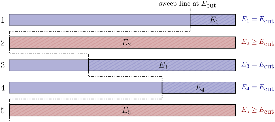
Figure 1: An illustration of the final state of the line sweep for an example with $5$ agents. As shown in the figure, agent $2$ and agent $5$ have a mean above the sweep line larger than $E_{\mathrm{cut}}$, as their quantile cuts satisfy $q_{i}=1$.

Now consider the scenario where the principalknows everyone’s exact value, and selects all agents $i$ whose value is above their own quantile cut $q_{i}$, and additionally selects $k$ agents with highest values among the remaining agents. The social welfare in this scenario is at most

$$\mathrm{SW}^{\prime}\leq E_{\mathrm{cut}}\cdot k+\sum_{i\in[N]}E_{i}\cdot q_{i}.$$

Since in this scenario the principalalways selects a (weak) superset of the agents selected under full-revelation of values (where the principalknows the revealed value of all agents and selects the top $k$ posterior mean agents), the social welfare achieved under full revelation of values $\mathrm{SW}^{\max}$ is at most $\mathrm{SW}^{\prime}$.

Lemma 5.2.

$\mathrm{SW}^{\max}\leq E_{\mathrm{cut}}\cdot k+\sum_{i\in[N]}E_{i}\cdot q_{i}$.

Consider any Nash equilibrium strategy profile $\bm{\mathcal{Z}}$. Denote the probability of agent $i$ being selected by

$$r_{i}(\bm{\mathcal{Z}})=\int_{\bigotimes_{i=1}^{N}\Sigma_{i}}\rho_{i}(\bm{\sigma})\mathop{\mathrm{d}\!}\bm{\Pi}(\bm{\sigma}).$$

Fix a constant $\alpha>1/Q$. Since $Q\leq 1$, we have $\alpha>1$. We group the agents into two sets $\mathcal{N}_{1}$ and $\mathcal{N}_{2}$ based on their $r_{i}(\bm{\mathcal{Z}})$ as:

$$\mathcal{N}_{1}=\{i\in[N]:r_{i}(\bm{\mathcal{Z}})\geq\alpha\cdot q_{i}\};\qquad\mathcal{N}_{2}=\{i\in[N]:r_{i}(\bm{\mathcal{Z}})<\alpha\cdot q_{i}\}.$$

Since $\sum_{i\in[N]}r_{i}(\bm{\mathcal{Z}})\leq k$, we have $\sum_{i\in\mathcal{N}_{1}}q_{i}\leq k/\alpha$. Therefore, $\sum_{i\in\mathcal{N}_{2}}q_{i}\geq(Q-1/\alpha)\cdot k$. Since $Q>1/\alpha$, $\mathcal{N}_{2}$ cannot be an empty set. We have the following simple lemma.

Lemma 5.3.

If $E_{i}>E_{\mathrm{cut}}$, then $i\in\mathcal{N}_{2}$. Therefore, $\min_{i\in\mathcal{N}_{2}}E_{i}\geq\max_{i\in\mathcal{N}_{1}}E_{i}$.

Proof.

When $E_{i}>E_{\mathrm{cut}}$, we have $q_{i}=1$. Since $\alpha>1$, this implies $\alpha\cdot q_{i}>1$. However, $r_{i}(\bm{\mathcal{Z}})\leq 1$, which means $i\in\mathcal{N}_{2}$. Since $E_{j}\geq E_{\mathrm{cut}}$ for all $j$, it must hold that $\max_{i\in\mathcal{N}_{1}}E_{i}=E_{\mathrm{cut}}$, completing the proof. ∎

In the rest of the analysis, we will fix a constant $\beta>0$. We split the analysis based on the value generated by agents in $\mathcal{N}_{2}$ when they are selected.

5.2 Case 1: All Agents in $\mathcal{N}_{2}$ are Large Contributors

For each agent $i$, define the value contribution of $i$ as

$$c_{i}(\bm{\mathcal{Z}})=\int_{\bigotimes_{i=1}^{N}\Sigma_{i}}\rho_{i}(\bm{\sigma})\cdot e_{i}(\sigma_{i})\mathop{\mathrm{d}\!}\bm{\Pi}(\bm{\sigma}),$$

where $e_{i}(\sigma_{i})$ is the posterior mean when agent $i$ sends signal $\sigma_{i}$.

Notice that the overall social welfare in equilibrium $\bm{\mathcal{Z}}$ is

$$\mathrm{SW}(\bm{\mathcal{Z}})=\sum_{i\in[N]}c_{i}(\bm{\mathcal{Z}}).$$

We prove that when all the agents in $\mathcal{N}_{2}$ have large value contribution, the social welfare of $\bm{\mathcal{Z}}$ is at least a constant fraction of the optimal social welfare.

Lemma 5.4.

Given a strategy profile $\bm{\mathcal{Z}}$, if all agents in $\mathcal{N}_{2}$ satisfy $c_{i}(\bm{\mathcal{Z}})\geq E_{i}\cdot\beta\cdot q_{i}$, then we have

$$\mathrm{SW}(\bm{\mathcal{Z}})\geq\mathrm{SW}^{\prime}\cdot\frac{\beta\cdot(Q-1/\alpha)}{1+Q}.$$

Proof.

We have

$$\mathrm{SW}(\bm{\mathcal{Z}}) =\sum_{i\in[N]}c_{i}\geq\sum_{i\in\mathcal{N}_{2}}c_{i}\geq\beta\cdot\sum_{i\in\mathcal{N}_{2}}E_{i}\cdot q_{i}$$

$$\geq\beta\cdot\left(\sum_{i\in[N]}q_{i}\cdot E_{i}\right)\cdot\frac{\sum_{i\in\mathcal{N}_{2}}q_{i}}{\sum_{i\in[N]}q_{i}}$$ (Lemma 5.3)

$$\geq\beta\cdot\left(\sum_{i\in[N]}q_{i}\cdot E_{i}+k\cdot E_{\mathrm{cut}}\right)\cdot\frac{\sum_{i\in[N]}q_{i}}{k+\sum_{i\in[N]}q_{i}}\cdot\frac{\sum_{i\in\mathcal{N}_{2}}q_{i}}{\sum_{i\in[N]}q_{i}} E_{i}\geq E_{\mathrm{cut}}$$ (Since for any agent)

$$\geq\beta\cdot\mathrm{SW}^{\prime}\cdot\frac{Q}{1+Q}\cdot\frac{Q-1/\alpha}{Q}=\mathrm{SW}^{\prime}\cdot\frac{\beta\cdot(Q-1/\alpha)}{1+Q}.$$

This completes the proof. ∎

Since $\mathrm{SW}^{\max}\leq\mathrm{SW}^{\prime}$, it follows that the Price of Anarchy is bounded by $\frac{1+Q}{\beta\cdot(Q-1/\alpha)}$ in this case.

5.3 Case 2: Some Agent in $\mathcal{N}_{2}$ Is a Small Contributor

Now assume that there exists an agent $i^{*}\in\mathcal{N}_{2}$ for which

$$c_{i^{*}}<E\cdot\beta\cdot q_{i^{*}}.$$

In other words, the agent $i^{*}$ is not selected with enough value from her equilibrium strategy. Our goal is to show that in this case, the agent $i^{*}$ can deviate in a way that will improve her payoff if the social welfare is too low, which contradicts the equilibrium condition.

Fix some constant $\phi>1$ and consider the top $\phi_{i^{*}}=\min\{\phi\cdot q_{i^{*}},\ 1\}$ quantile of $i^{*}$’s value distribution. Let $\bm{\Pi}_{-i^{*}}=\bigotimes_{j\neq i^{*}}\Pi_{j}$ denote the distribution of signals from all agents except $i^{*}$. For simplicity, for any signal profile $\bm{\sigma}$, we write $\rho_{i^{*}}(\bm{\sigma})$ as $\rho_{i^{*}}(\sigma_{i^{*}},\bm{\sigma}_{-i^{*}})$ where $\bm{\sigma}_{-i^{*}}$ is the signal profile of all agents except $i^{*}$. For each signal $\sigma_{i^{*}}\in\Sigma_{i^{*}}$, define

$$w_{i^{*}}(\sigma_{i^{*}})=\int_{\bigotimes_{j\neq i^{*}}\Sigma_{j}}\rho_{i^{*}}(\sigma_{i^{*}},\bm{\sigma}_{-i^{*}})\mathop{\mathrm{d}\!}\bm{\Pi}_{-i^{*}}(\bm{\sigma}_{-i^{*}}).$$

This represents the overall probability that agent $i^{*}$ is selected when she sends the signal $\sigma_{i^{*}}$.

5.3.1 Construction of the deviation signal $s^{*}$

This step is the key to the analysis. Choose a constant $\tau\in(0,1)$. We partition the signals of $\Sigma_{i^{*}}$ into two sets:

$$S_{1}=\{\sigma\in\Sigma_{i^{*}}:w_{i^{*}}(\sigma)\geq\tau\},\text{ and }S_{2}=\{\sigma\in\Sigma_{i^{*}}:w_{i^{*}}(\sigma)<\tau\}.$$

Here, $S_{1}$ consists of signals that yield a high probability (at least $\tau$) of agent $i^{*}$ being selected, while $S_{2}$ contains signals with low probabilities of being selected.

We construct a new signaling scheme $\mathcal{Z}_{i^{*}}^{\prime}=\{\Sigma_{i^{*}}\cup\{s^{*}\},\pi_{i^{*}}^{\prime}\}$ of agent $i^{*}$. The signaling scheme adds a new signal $s^{*}$ to the original signal space $\Sigma_{i^{*}}$. The new signal $s^{*}$ is formed by merging all the value mass in the top $\phi_{i^{*}}$ quantile that were originally mapped to $S_{2}$. Formally, for any measurable set $S\subseteq\Sigma_{i^{*}}^{\prime}$ and for each $v\in V$, $\pi_{i^{*}}(S\mid v)$ is given by:

$$\pi_{i^{*}}^{\prime}(S\mid v)=\begin{cases}\pi_{i^{*}}(S\cap S_{1}\mid v)+\pi_{i^{*}}(S_{2}\mid v)\cdot\mathbb{1}[s^{*}\in S]&\text{if $v$ is in the top $\phi_{i^{*}}$-quantile of $\mathcal{F}_{i^{*}}$,}\\ \pi_{i^{*}}(S\mid v)&\text{otherwise.}\end{cases}$$

The intuition of our construction is that we are “recombining” all the signals in $S_{2}$ that come from the high-value region into one single signal $s^{*}$. This new signal is intended to improve agent $i^{*}$’s chances of being selected on higher values by eliminating the low probabilities of being selected that were associated with signals in $S_{2}$.

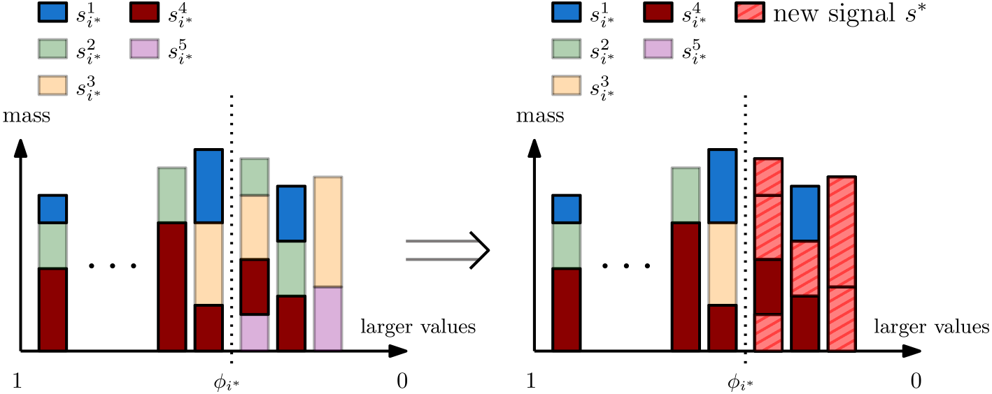
Figure 2: Illustration of construction of deviation signaling scheme $s^{*}$.

Fig.˜2 illustrates the process of the construction of $s^{*}$. The $x$-axis represents the values while the $y$-axis (heights of the bars) represents the mass on the corresponding values. Since each signal consists of masses on different values, we use the same color set of rectangles to represent a signal. In the illustration, we assume $\Sigma_{i^{*}}$ consists of five signals $\{s_{i^{*}}^{j}\}_{j=1}^{5}$. Assume that if signal $s_{i^{*}}^{1}$ or $s_{i^{*}}^{4}$ is sent, agent $i^{*}$ has at least $\tau$ probability of being selected. Then $s_{i^{*}}^{1},s_{i^{*}}^{4}\in S_{1}$. On the other hand, $s_{i^{*}}^{2}$, $s_{i^{*}}^{3}$, or $s_{i^{*}}^{5}$ belong to $S_{2}$. We will pick all the masses from by these signals with values in the top $\phi_{i^{*}}$ quantile, and combine them into a signal $s^{*}$, as shown in the tiled area on the right.

5.3.2 The posterior mean of $s^{*}$

Let $e_{i^{*}}(\sigma)$ denote the posterior mean of signal $\sigma$ under agent $i^{*}$’s original signaling scheme $\mathcal{Z}_{i^{*}}$, and let $e_{i^{*}}^{\prime}(s^{*})$ denote the posterior mean of the new signal $s^{*}$ under $\mathcal{Z}_{i^{*}}^{\prime}$. We will first show that the posterior mean of $s^{*}$ is at least a constant fraction of $E_{i^{*}}$.

Lemma 5.5.

$e_{i^{*}}^{\prime}(s^{*})\geq E_{i^{*}}\cdot\left(\frac{1}{\phi}-\frac{\beta}{\tau\cdot\phi}\right)$.

Proof.

Since $c_{i^{*}}<E_{i^{*}}\cdot\beta\cdot q_{i^{*}}$, the value contribution comes from signals in $S_{1}$ or signals in $S_{2}$. Therefore, by considering only signals in $S_{1}$, we have

$$\int_{\sigma\in S_{1}}e_{i^{*}}(\sigma)\cdot w_{i^{*}}(\sigma)\mathop{\mathrm{d}\!}\,\Pi_{i^{*}}(\sigma)<E_{i^{*}}\cdot\beta\cdot q_{i^{*}}.$$

By definition of $S_{1}$, for all $\sigma\in S_{1}$, $w_{i^{*}}(\sigma)>\tau$. We have

$$\int_{\sigma\in S_{1}}e_{i^{*}}(\sigma)\mathop{\mathrm{d}\!}\,\Pi_{i^{*}}(\sigma)<\frac{E_{i^{*}}\cdot\beta\cdot q_{i^{*}}}{\tau}.$$ (4)

Since $s^{*}$ and the signals in $S_{1}$ must have “used up” all the masses in the top $\phi_{i^{*}}$ quantile of $\mathcal{F}_{i^{*}}$, we have

$$\int_{\sigma\in S_{1}}e_{i^{*}}(\sigma)\mathop{\mathrm{d}\!}\,\Pi_{i^{*}}(\sigma)+e_{i^{*}}^{\prime}(s^{*})\cdot\Pr[\textrm{$s^{*}$ is sent}]\geq E_{i^{*}}\cdot q_{i^{*}}.$$ (5)

Since $s^{*}$ is sent only when agent $i^{*}$’s value is in the top $\phi_{i^{*}}$ quantile, it must hold that $0<\Pr[\textrm{$s^{*}$ is sent}]\leq\phi\cdot q_{i^{*}}$. Combining with Eqs.˜4 and 5, we have

$$e_{i^{*}}^{\prime}(s^{*})\geq\frac{E_{i^{*}}\cdot q_{i^{*}}-\frac{E_{i^{*}}\cdot\beta\cdot q_{i^{*}}}{\tau}}{\phi\cdot q_{i^{*}}}\geq E_{i^{*}}\cdot\left(\frac{1}{\phi}-\frac{\beta}{\tau\cdot\phi}\right),$$

completing the proof. ∎

5.3.3 Deviation to $s^{*}$ in new signaling scheme

Denote by $\bm{\mathcal{Z}}^{\prime}$ the signaling scheme profile where only agent $i^{*}$ deviates to the new signaling scheme $\mathcal{Z}_{i^{*}}^{\prime}$ while all other agents keep their signaling scheme in $\bm{\mathcal{Z}}$.

Lemma 5.6.

Assuming $\phi\cdot\tau>\alpha,$ in the new signaling scheme profile $\bm{\mathcal{Z}}^{\prime}$, we have

$$\Pr[i^{*}\mbox{ is selected}\mid s^{*}\mbox{ is sent}]<\tau.$$

Proof.

Assume instead that when signal $s^{*}$ is sent, agent $i^{*}$ is selected with probability at least $\tau$. Since $\phi_{i^{*}}=\min(1,\phi\cdot q_{i^{*}})$, we consider the following two cases:

• If $\phi_{i^{*}}=1$, then agent $i^{*}$’s deviation to $s^{*}$ strictly increases the probability of being selected on all values used to form $s^{*}$, since their original probability of being selected is less than $\tau$ by definition of $S_{2}$. Therefore, agent $i^{*}$ will strictly benefit from the deviation.

• If $\phi_{i^{*}}=\phi\cdot q_{i^{*}}$, consider the case after agent $i^{*}$ deviates to $\mathcal{Z}_{i^{*}}^{\prime}$. All values in the top $(\phi\cdot q_{i^{*}})$ quantile are mapped to either signals in $S_{1}$ or $s^{*}$. Since when any signal in $S_{1}$ or $s^{*}$ is sent to the principal, agent $i^{*}$ is selected with probability at least $\tau$, the deviation to $s^{*}$ makes her overall probability of being selected at least $\phi\cdot q_{i^{*}}\cdot\tau$. By the construction of $\mathcal{Z}_{i^{*}}$, agent $i^{*}$ loses utility from the cases when her value is at most $v_{i^{*}}(\phi_{i^{*}})$ and gains utility from the cases when her value is at least $v_{i^{*}}(\phi_{i^{*}})$. Recall that $i^{*}\in\mathcal{N}_{2}$, so $r_{i^{*}}(\bm{\mathcal{Z}})<\alpha\cdot q_{i^{*}}$. Since the parameters satisfy $\phi\cdot\tau>\alpha$, agent $i^{*}$’s overall probability of being selected increases from strictly less than $\alpha\cdot q_{i^{*}}$ to $\phi\cdot\tau\cdot q_{i^{*}}$. She will gain at least

  $$(\phi\cdot\tau-\alpha)\cdot q_{i^{*}}\cdot u_{i^{*}}(v_{i^{*}}(\phi_{i^{*}}))>0$$

  additional utility from the deviation.

Therefore, agent $i^{*}$ will strictly benefit from the potential strategy deviation from $\mathcal{Z}_{i^{*}}$ to $\mathcal{Z}_{i^{*}}^{\prime}$, which contradicts the fact that $\bm{\mathcal{Z}}$ is a Nash equilibrium. ∎

By the above lemma, we can assume that in $\bm{\mathcal{Z}}^{\prime}$, agent $i^{*}$ is selected with probability strictly less than $\tau$ when $s^{*}$ is sent. We now classify all agents into two groups $\mathcal{N}_{\ell}$ and $\mathcal{N}_{s}$, according to whether an agent $i$ has $E_{i}$ larger or smaller than $E_{i^{*}}$:

$$\mathcal{N}_{\ell}=\{i\in[N]:E_{i}>E_{i^{*}}\};\qquad\mathcal{N}_{s}=\{i\in[N]:E_{i}\leq E_{i^{*}}\}.$$

Since $E_{i^{*}}\geq E_{\mathrm{cut}}$, all agents in $\mathcal{N}_{\ell}$ must have their $q_{i}=1$. Note that $i^{*}\in\mathcal{N}_{s}$. Since $q_{i^{*}}>0$ and $\sum_{i\in[N]}q_{i}=Q\cdot k$, we have $|\mathcal{N}_{\ell}|<k\cdot Q\leq k$, where we have used $Q\leq 1$.

Let $M(\bm{\mathcal{Z}})$ denote the random variable indicating the $(k-|\mathcal{N}_{\ell}|)$-th largest posterior mean among all agents in $\mathcal{N}_{s}$ in the Nash equilibrium $\bm{\mathcal{Z}}$.

Lemma 5.7.

If agent $i^{*}$ is selected with probability less than $\tau$ when $s^{*}$ is sent in $\bm{\mathcal{Z}}^{\prime}$, we have

$$\Pr[M(\bm{\mathcal{Z}})\geq e_{i^{*}}(s^{*})]\geq 1-\tau.$$

Proof.

If not, we have $\Pr[M(\bm{\mathcal{Z}})\geq e_{i^{*}}(s^{*})]<1-\tau\Rightarrow\Pr[M(\bm{\mathcal{Z}})<e_{i^{*}}(s^{*})]\geq\tau$. Denote by $M_{-i^{*}}(\bm{\mathcal{Z}})$ the random variable representing the $(k-|\mathcal{N}_{\ell}|)$-th largest posterior mean among all agents except $i^{*}$ in $\mathcal{N}_{s}$ in $\bm{\mathcal{Z}}$. $M_{-i^{*}}(\bm{\mathcal{Z}})$ is stochastically dominated by $M(\bm{\mathcal{Z}})$. When $M_{-i^{*}}(\bm{\mathcal{Z}})<e_{i^{*}}(s^{*})$, agent $i^{*}$ must be selected when $s^{*}$ is sent. This contradicts the assumption that she is selected with probability less than $\tau$ when $s^{*}$ is selected. ∎

We first present a proof showing that when the top $(1-\tau)$ quantile of $M(\bm{\mathcal{Z}})$ is no less than the posterior mean of $s^{*}$, the social welfare decreases by at most a constant.

Lemma 5.8.

Given a strategy profile $\bm{\mathcal{Z}}$, if $\Pr\left[M(\bm{\mathcal{Z}})\geq e_{i^{*}}(s^{*})\right]\geq 1-\tau$, then we have

$$\mathrm{SW}(\bm{\mathcal{Z}})\geq\mathrm{SW}^{\prime}(\bm{\mathcal{Z}})\cdot\frac{(1-\tau)\cdot\left(\frac{1}{\phi}-\frac{\beta}{\tau\cdot\phi}\right)}{1+Q}.$$

Proof.

Consider a hypothetical scenario where, instead of selecting the $k$ agents with the highest posterior means, the principalselects all agents in $\mathcal{N}_{\ell}$ and selects the remaining $k-|\mathcal{N}_{\ell}|$ agents from $\mathcal{N}_{s}$ with the highest posterior means. Denote the resulting social welfare in this scenario by $\mathrm{SW}^{\textrm{(fake)}}$. We have

$$\mathrm{SW}^{\textrm{(fake)}}(\bm{\mathcal{Z}}) \geq(k-|\mathcal{N}_{l}|)\cdot\mathbb{E}[M(\bm{\mathcal{Z}})]+\sum_{i\in\mathcal{N}_{\ell}}E_{i}$$

$$\geq(1-\tau)\cdot(k-|\mathcal{N}_{l}|)\cdot e_{i^{*}}(s^{*})+\sum_{i\in\mathcal{N}_{\ell}}E_{i} 1-\tau M(\bm{\mathcal{Z}})\geq e_{i^{*}}(s^{*})$$ (w.p. , . )

$$\geq(1-\tau)\cdot(k-|\mathcal{N}_{\ell}|)\cdot\left(\frac{1}{\phi}-\frac{\beta}{\tau\cdot\phi}\right)\cdot E_{i^{*}}+\sum_{i\in\mathcal{N}_{\ell}}E_{i}$$ (Lemma 5.5)

$$\geq\frac{(1-\tau)\cdot(k-|\mathcal{N}_{\ell}|)\cdot\left(\frac{1}{\phi}-\frac{\beta}{\tau\cdot\phi}\right)\cdot E_{i^{*}}+\sum_{i\in\mathcal{N}_{\ell}}E_{i}}{(1-\tau)\cdot\left(\frac{1}{\phi}-\frac{\beta}{\tau\cdot\phi}\right)\cdot(k-|\mathcal{N}_{\ell}|)+|\mathcal{N}_{\ell}|}\cdot(1-\tau)\cdot\left(\frac{1}{\phi}-\frac{\beta}{\tau\cdot\phi}\right)\cdot k.$$ (6)

To see the last inequality, note that $Q\leq 1$, so that $\alpha>\frac{1}{Q}\geq 1$. Since $\tau<1$, we have $\phi\geq\frac{\alpha}{\tau}>1$. Since $\beta\leq\tau$, we finally have

$$(1-\tau)\cdot\left(\frac{1}{\phi}-\frac{\beta}{\tau\cdot\phi}\right)\leq(1-\tau)<1.$$

Hence,

$$(1-\tau)\cdot\left(\frac{1}{\phi}-\frac{\beta}{\tau\cdot\phi}\right)\cdot(k-|\mathcal{N}_{\ell}|)+|\mathcal{N}_{\ell}|\geq(1-\tau)\cdot\left(\frac{1}{\phi}-\frac{\beta}{\tau\cdot\phi}\right)\cdot k.$$

Since $E_{\mathrm{cut}}\leq E_{i}\leq E_{i^{*}}\leq E_{j}$, for any $i\in\mathcal{N}_{s}$, and $j\in\mathcal{N}_{\ell}$, it follows that any convex combination of $E_{\mathrm{cut}}$ and $\{E_{i}\}_{i\in\mathcal{N}_{s}}$ cannot exceed $E_{i^{*}}$, while $E_{i^{*}}$ cannot exceed any convex combination of $\{E_{j}\}_{j\in\mathcal{N}_{\ell}}$. Therefore,

$$\frac{k\cdot E_{\mathrm{cut}}+\sum_{i\in\mathcal{N}_{s}}E_{i}\cdot q_{i}}{k+\sum_{i\in\mathcal{N}_{s}}q_{i}}\leq E_{i^{*}}\leq\frac{\sum_{i\in\mathcal{N}_{\ell}}E_{i}}{|\mathcal{N}_{\ell}|}.$$

For any real numbers $b\geq a_{\ell}\geq a_{s}\geq 0,w_{\ell}\geq w_{s},w_{b}\geq 0$, we have

$$\frac{a_{\ell}\cdot w_{s}+b\cdot w_{b}}{w_{s}+w_{b}}\geq\frac{a_{s}\cdot w_{\ell}+b\cdot w_{b}}{w_{\ell}+w_{b}}.$$

By letting $b=\frac{\sum_{i\in\mathcal{N}_{\ell}}E_{i}}{|\mathcal{N}_{\ell}|}$, $w_{b}=|\mathcal{N}_{\ell}|$, $a_{\ell}=E_{i^{*}}$, $w_{s}=(1-\tau)\cdot\left(\frac{1}{\phi}-\frac{\beta}{\tau\cdot\phi}\right)\cdot(k-|\mathcal{N}_{\ell}|)$, $a_{s}=\frac{k\cdot E_{\mathrm{cut}}+\sum_{i\in\mathcal{N}_{s}}E_{i}\cdot q_{i}}{k+\sum_{i\in\mathcal{N}_{s}}q_{i}}$, $w_{\ell}=k+\sum_{i\in\mathcal{N}_{s}}q_{i}$, it follows from Eq.˜6 that

$$\mathrm{SW}^{\textrm{(fake)}}(\bm{\mathcal{Z}}) \geq\frac{k\cdot E_{\mathrm{cut}}+\sum_{i\in\mathcal{N}_{s}}E_{i}\cdot q_{i}+\sum_{i\in\mathcal{N}_{\ell}}E_{i}}{k+\sum_{i\in\mathcal{N}_{s}}q_{i}+|\mathcal{N}_{\ell}|}\cdot(1-\tau)\cdot\left(\frac{1}{\phi}-\frac{\beta}{\tau\cdot\phi}\right)\cdot k$$

$$=\frac{\mathrm{SW}^{\prime}}{(1+Q)\cdot k}\cdot(1-\tau)\cdot\left(\frac{1}{\phi}-\frac{\beta}{\tau\cdot\phi}\right)\cdot k.$$

Since in the fake scenario, the principalmay not be a posterior mean maximizer, we have $\mathrm{SW}^{\textrm{(fake)}}(\bm{\mathcal{Z}})\leq\mathrm{SW}(\bm{\mathcal{Z}})$. This completes the proof. ∎

Since $\mathrm{SW}^{\prime}$ is an upper bound on social welfare in the full-revelation scenario, and since selection in the hypothetical scenario leads to at most the social welfare of selecting the $k$ agents with highest posterior mean, the PoA in this case is at most $\frac{1+Q}{(1-\tau)\cdot\left(\frac{1}{\phi}-\frac{\beta}{\tau\cdot\phi}\right)}$.

Completing the proof of Theorem˜5.1.

Since either Case 1 or Case 2 happens, the PoA is at most

$$\mbox{PoA}\leq\max\left\{\frac{1+Q}{\beta\cdot(Q-1/\alpha)},\frac{1+Q}{(1-\tau)\cdot\left(\frac{1}{\phi}-\frac{\beta}{\tau\cdot\phi}\right)}\right\}.$$

By setting

$$Q=1,\qquad\alpha=\frac{\sqrt{5}+1}{2}\approx 1.618,\qquad\beta=\sqrt{5}-2\approx 0.236,$$

$$\tau=\frac{\sqrt{5}-1}{2}\approx 0.618,\qquad\phi=\frac{\sqrt{5}+3}{2}\approx 2.618,$$

we know that the PoA of any instance is at most $11+5\sqrt{5}\approx 22.18$. This completes the proof of Theorem˜5.1. ∎

6 Open Questions

There are several avenues for future research. The immediate question is to improve the constant factor in Theorem˜5.1; this will require new ideas. Another open question is to show the existence of a Nash equilibrium in the most general model considered in Section˜5. Though the existence is known for the non-identical prior version of the utility model in Section˜4, extending this result to all utility functions would be non-trivial and interesting. Further, it would be interesting to extend our results further to the setting where the principal solves an arbitrary combinatorial optimization problem on the agents, and when agent values can be multi-dimensional. As an example, each agent can control a subset of edges in a graph, whose cost they seek to signal to the principal, while the principal seeks to compute a minimum spanning tree on these edges. Another example is the price discrimination setting in Bergemann et al. (2015). Finally, it would be interesting to explore PoA for other models of information revelation beyond signaling, for instance, models where the agents themselves are uncertain about their values (Roesler and Szentes, 2017).

References

- Alijani et al. [2022] Reza Alijani, Siddhartha Banerjee, Kamesh Munagala, and Kangning Wang. The limits of an information intermediary in auction design. In Proceedings of the 23rd ACM Conference on Economics and Computation (EC), pages 849–868. ACM, 2022.
- Anshelevich et al. [2008] Elliot Anshelevich, Anirban Dasgupta, Jon Kleinberg, Éva Tardos, Tom Wexler, and Tim Roughgarden. The price of stability for network design with fair cost allocation. SIAM J. Comput., 38(4):1602–1623, November 2008. ISSN 0097-5397. doi:10.1137/070680096. URL https://doi.org/10.1137/070680096.
- Au and Kawai [2020] Pak Hung Au and Keiichi Kawai. Competitive information disclosure by multiple senders. Games and Economic Behavior, 119:56–78, 2020.
- Au and Kawai [2021] Pak Hung Au and Keiichi Kawai. Competitive disclosure of correlated information. Economic Theory, 72(3):767–799, 2021.
- Babaioff et al. [2020] Moshe Babaioff, Nicole Immorlica, Brendan Lucier, and S. Matthew Weinberg. A simple and approximately optimal mechanism for an additive buyer. J. ACM, 67(4), June 2020. ISSN 0004-5411. doi:10.1145/3398745. URL https://doi.org/10.1145/3398745.
- Babichenko et al. [2021] Yakov Babichenko, Inbal Talgam-Cohen, Haifeng Xu, and Konstantin Zabarnyi. Regret-minimizing bayesian persuasion. In Proceedings of the 22nd ACM Conference on Economics and Computation (EC), page 128. ACM, 2021. doi:10.1145/3465456.3467574. URL https://doi.org/10.1145/3465456.3467574.
- Banerjee et al. [2024] Siddhartha Banerjee, Kamesh Munagala, Yiheng Shen, and Kangning Wang. Fair price discrimination. In Proceedings of the 2024 ACM-SIAM Symposium on Discrete Algorithms (SODA), pages 2679–2703. SIAM, 2024. doi:10.1137/1.9781611977912.96. URL https://doi.org/10.1137/1.9781611977912.96.
- Banerjee et al. [2025] Siddhartha Banerjee, Kamesh Munagala, Yiheng Shen, and Kangning Wang. Majorized bayesian persuasion and fair selection. In Proceedings of the 2025 Annual ACM-SIAM Symposium on Discrete Algorithms (SODA), pages 1837–1856. SIAM, 2025.
- Bergemann and Morris [2019] Dirk Bergemann and Stephen Morris. Information design: A unified perspective. Journal of Economic Literature, 57(1):44–95, 2019.
- Bergemann et al. [2015] Dirk Bergemann, Benjamin Brooks, and Stephen Morris. The limits of price discrimination. American Economic Review, 105(3):921–957, 2015.
- Boleslavsky and Cotton [2015] Raphael Boleslavsky and Christopher Cotton. Grading standards and education quality. American Economic Journal: Microeconomics, 7(2):248–279, 2015.
- Boleslavsky and Cotton [2018] Raphael Boleslavsky and Christopher Cotton. Limited capacity in project selection: Competition through evidence production. Economic Theory, 65:385–421, 2018.
- Cummings et al. [2020] Rachel Cummings, Nikhil R. Devanur, Zhiyi Huang, and Xiangning Wang. Algorithmic price discrimination. In Proceedings of the 2020 ACM-SIAM Symposium on Discrete Algorithms (SODA), pages 2432–2451. SIAM, 2020. doi:10.1137/1.9781611975994.149. URL https://doi.org/10.1137/1.9781611975994.149.
- Devic et al. [2024] Siddartha Devic, Aleksandra Korolova, David Kempe, and Vatsal Sharan. Stability and multigroup fairness in ranking with uncertain predictions. In Proceedings of the 41st International Conference on Machine Learning (ICML). PMLR, 2024.
- Ding et al. [2023] Bolin Ding, Yiding Feng, Chien-Ju Ho, Wei Tang, and Haifeng Xu. Competitive information design for pandora’s box. In Proceedings of the 2023 Annual ACM-SIAM Symposium on Discrete Algorithms (SODA), pages 353–381. SIAM, 2023.
- Dixon-Román et al. [2013] Ezekiel J. Dixon-Román, Howard T. Everson, and John J. McArdle. Race, poverty and SAT scores: Modeling the influences of family income on black and white high school students’ SAT performance. Teachers College Record, 115(4):1–33, 2013.
- Du et al. [2024] Zhicheng Du, Wei Tang, Zihe Wang, and Shuo Zhang. Competitive information design with asymmetric senders. In Proceedings of the 25th ACM Conference on Economics and Computation (EC), 2024.
- Dughmi [2017] Shaddin Dughmi. Algorithmic information structure design: a survey. SIGecom Exchanges, 15(2):2–24, 2017. doi:10.1145/3055589.3055591. URL https://doi.org/10.1145/3055589.3055591.
- Dughmi and Xu [2016] Shaddin Dughmi and Haifeng Xu. Algorithmic bayesian persuasion. In Daniel Wichs and Yishay Mansour, editors, Proceedings of the 48th Annual ACM SIGACT Symposium on Theory of Computing (STOC), pages 412–425. ACM, 2016. doi:10.1145/2897518.2897583. URL https://doi.org/10.1145/2897518.2897583.
- Emelianov et al. [2020] Vitalii Emelianov, Nicolas Gast, Krishna P. Gummadi, and Patrick Loiseau. On fair selection in the presence of implicit variance. In Proceedings of the 21st ACM Conference on Economics and Computation (EC), pages 649–675. ACM, 2020. doi:10.1145/3391403.3399482. URL https://doi.org/10.1145/3391403.3399482.
- García-Soriano and Bonchi [2021] David García-Soriano and Francesco Bonchi. Maxmin-fair ranking: Individual fairness under group-fairness constraints. In Proceedings of 27th ACM SIGKDD Conference on Knowledge Discovery and Data Mining (KDD), pages 436–446. ACM, 2021. doi:10.1145/3447548.3467349. URL https://doi.org/10.1145/3447548.3467349.
- Gentzkow and Kamenica [2016] Matthew Gentzkow and Emir Kamenica. Competition in persuasion. The Review of Economic Studies, 84(1):300–322, 2016.
- Gentzkow and Kamenica [2017] Matthew Gentzkow and Emir Kamenica. Bayesian persuasion with multiple senders and rich signal spaces. Games and Economic Behavior, 104:411–429, 2017.
- Gradwohl et al. [2022] Ronen Gradwohl, Niklas Hahn, Martin Hoefer, and Rann Smorodinsky. Reaping the informational surplus in bayesian persuasion. American Economic Journal: Microeconomics, 14(4):296–317, 2022.
- Hartline et al. [2014] Jason Hartline, Darrell Hoy, and Sam Taggart. Price of anarchy for auction revenue. In Proceedings of the Fifteenth ACM Conference on Economics and Computation (EC), page 693–710. ACM, 2014. ISBN 9781450325653. doi:10.1145/2600057.2602878. URL https://doi.org/10.1145/2600057.2602878.
- Hoffmann et al. [2020] Florian Hoffmann, Roman Inderst, and Marco Ottaviani. Persuasion through selective disclosure: Implications for marketing, campaigning, and privacy regulation. Management Science, 66(11):4958–4979, 2020.
- Hossain et al. [2024] Safwan Hossain, Tonghan Wang, Tao Lin, Yiling Chen, David C. Parkes, and Haifeng Xu. Multi-sender persuasion: A computational perspective. In Proceedings of the 41st International Conference on Machine Learning (ICML), 2024.
- Hwang et al. [2019] Ilwoo Hwang, Kyungmin Kim, and Raphael Boleslavsky. Competitive advertising and pricing. Emory University and University of Miami, 2019.
- Jain and Whitmeyer [2019] Vasudha Jain and Mark Whitmeyer. Competing to persuade a rationally inattentive agent. arXiv preprint arXiv:1907.09255, 2019.
- Kamenica and Gentzkow [2011] Emir Kamenica and Matthew Gentzkow. Bayesian persuasion. American Economic Review, 101(6):2590–2615, 2011.
- Krengel and Sucheston [1978] Ulrich Krengel and Louis Sucheston. On semiamarts, amarts, and processes with finite value. In Probability on Banach spaces, volume 4 of Adv. Probab. Related Topics, pages 197–266. Dekker, New York, 1978. ISBN 0-8247-6799-3.
- Mehrotra and Celis [2021] Anay Mehrotra and L. Elisa Celis. Mitigating bias in set selection with noisy protected attributes. In Proceedings of the 2021 ACM Conference on Fairness, Accountability, and Transparency (FAccT), pages 237–248. ACM, 2021. doi:10.1145/3442188.3445887. URL https://doi.org/10.1145/3442188.3445887.
- Ravindran and Cui [2020] Dilip Ravindran and Zhihan Cui. Competing persuaders in zero-sum games. arXiv preprint arXiv:2008.08517, 2020.
- Roesler and Szentes [2017] Anne-Katrin Roesler and Balázs Szentes. Buyer-optimal learning and monopoly pricing. American Economic Review, 107(7):2072–80, July 2017. doi:10.1257/aer.20160145. URL https://www.aeaweb.org/articles?id=10.1257/aer.20160145.
- Roughgarden [2015] Tim Roughgarden. Intrinsic robustness of the price of anarchy. J. ACM, 62(5), November 2015. ISSN 0004-5411. doi:10.1145/2806883. URL https://doi.org/10.1145/2806883.
- Sapiro-Gheiler [2024] Eitan Sapiro-Gheiler. Persuasion with ambiguous receiver preferences. Economic Theory, 77(4):1173–1218, 2024.
- Shen et al. [2023] Zeyu Shen, Zhiyi Wang, Xingyu Zhu, Brandon Fain, and Kamesh Munagala. Fairness in the assignment problem with uncertain priorities. In Proceedings of the 2023 International Conference on Autonomous Agents and Multiagent Systems (AAMAS), pages 188–196. ACM, 2023. doi:10.5555/3545946.3598636. URL https://dl.acm.org/doi/10.5555/3545946.3598636.
- Singh et al. [2021] Ashudeep Singh, David Kempe, and Thorsten Joachims. Fairness in ranking under uncertainty. In Proceedings of the 35th Annual Conference on Neural Information Processing Systems (NeurIPS), pages 11896–11908, 2021. URL https://proceedings.neurips.cc/paper/2021/hash/63c3ddcc7b23daa1e42dc41f9a44a873-Abstract.html.
- Xu et al. [2015] Haifeng Xu, Zinovi Rabinovich, Shaddin Dughmi, and Milind Tambe. Exploring information asymmetry in two-stage security games. In Proceedings of the 29th AAAI Conference on Artificial Intelligence (AAAI), pages 1057–1063. AAAI Press, 2015. doi:10.1609/AAAI.V29I1.9290. URL https://doi.org/10.1609/aaai.v29i1.9290.