UT-Komaba/24-8, YITP-24-155

Holographic Entanglement Entropy in the ​ FLRW Universe

Toshifumi Noumi^†, Fumiya Sano^♭,♮ and Yu-ki Suzuki^♯

^† Graduate School of Arts and Sciences, The University of Tokyo, Tokyo 153-8902, Japan

^♭ Department of Physics, Institute of Science Tokyo, Tokyo 152-8551, Japan

^♮ Center for Theoretical Physics of the Universe, Institute for Basic Science,
Daejeon 34126, Korea

^♯Center for Gravitational Physics and Quantum Information,
Yukawa Institute for Theoretical Physics, Kyoto University,
Kitashirakawa Oiwakecho, Sakyo-ku, Kyoto 606-8502, Japan

Abstract

We compute a holographic entanglement entropy via Ryu–Takayanagi prescription in the three-dimensional Friedmann–Lemaître–Robertson–Walker universe. We consider two types of holographic scenarios analogous to the static patch holography and the half de Sitter holography, in which the holographic boundary is timelike and placed in the bulk. We find in general that the strong subadditivity can be satisfied only in the former type and in addition the holographic boundary has to fit inside the apparent horizon. Also, for the universe filled with an ideal fluid of constant equation of state $w<-1$, the condition is sharpened as that the holographic boundary has to fit inside the event horizon instead. These conditions provide a necessary condition for the dual quantum field theory to be standard and compatible with the strong subadditivity.

1 Introduction and summary

After the discovery of the AdS/CFT (Anti-de Sitter/Conformal field theory) correspondence [1], theoretical physicists have been trying to understand the emergence of spacetime. One prominent way is to utilize quantum information theory in the AdS/CFT correspondence. The celebrated Ryu–Takayanagi (RT) formula [2, 3] proposed a gravity dual of entanglement entropy that can be regarded as a natural extension of Bekenstein–Hawking entropy [4, 5]. In the slogan of “It from Qubit”, which states that the spacetime emerges through quantum entanglement, we have been understanding quantum gravity in the AdS space.

An extension of the holographic principle to the de Sitter (dS) space, called the dS/CFT correspondence, was initiated by Strominger in Ref. [6]. Although dS/CFT is not indicated from the string theory unlike the AdS/CFT case, we can study various issues by assuming the would-be correspondence in the bottom-up spirit. For example, in the original dS/CFT correspondence [6], the dual CFT is on the future infinity of the de Sitter space and hence it does not admit the time direction. The resulting CFT is expected to be non-unitary, which can also be expected from the analytic continuation of the radius from the AdS case.

From the viewpoint of cosmology, the de Sitter space is directly related with our universe through cosmic inflation [7, 8, 9, 10], which is approximated by quasi-de Sitter space with broken time-translational symmetry due to the scalar field inflaton driving inflation. Correlation functions of the inflaton and graviton perturbations on the future infinity provide initial conditions for late-time anisotropy and inhomogeneity, which is observable through cosmic microwave background, large scale structures, and so on (see [11] for current constraints). Besides bulk analyses of inflationary perturbations, studies of inflationary correlators in the context of dS/CFT correspondence have been performed. Following pioneer works [12, 13, 14, 15], some phenomenological aspects have been discussed such as operator product expansion for non-Gaussian inflationary correlators [16], correspondence of slow-roll inflation/deformed CFT [17, 18, 19], initial vacuum states for wavefunction [20, 21] etc., as well as the so-called cosmological bootstrap [22, 23, 24, 25]. However, due to unhealthy dual CFT, as well as the additional complexity from broken de Sitter isometry during inflation, practical use of dS/CFT correspondence is basically limited to reproductions of some simple results of quantum field theory (QFT) in (quasi-)dS space.

Instead, to realize a QFT dual with time direction as in the AdS/CFT correspondence, we introduce a timelike holographic boundary (or also called a stretched horizon) as proposed in Refs. [26, 27] (see related works [28, 29, 30]). We impose the Dirichlet-like boundary conditions on the metric so that the dual QFT should be decoupled from bulk gravitational modes. In these cases, the bulk gravity is expected to be dual to a non-gravitating quantum field theory on the stretched horizon. The QFT may signal non-local behavior [27] since it is a finite-cutoff holography as in the $T\bar{T}$-deformation case [31, 32] (also see [33] for a relation to the violation of the strong subadditivity of the holographic entanglement entropy), but it is believed to be unitary. In these cases, the holographic boundary is not placed at the asymptotic boundary, and it is not clear where we should place the holographic boundary from the first principle.

An extension of the holographic principle to other general (closed) Friedmann–Lemaître–Robertson–Walker (FLRW) spacetime is recently proposed in Refs. [34, 35, 36], which shed light on the possibility that the entire history of our universe can be understood via holography and we can analyze scientifically why our universe is chosen from enormous possibilities.

In this paper we would like to discuss the following question: where should we place the holographic boundary and are there any holographic principles in the FLRW universe? We assume that the RT-prescription works in these spacetimes and explore constraints on holographic scenarios and background spacetimes by analyzing inequalities that the entanglement entropy should satisfy. More specifically, we compute the holographic entanglement entropy via the RT formula in three-dimensional flat, closed, and open FLRW spacetimes and analyze whether the strong subadditivity (SSA) is satisfied. We also use the ideal fluid approximation for the matter and label the FLRW spacetime by $w$, which relates the energy density $\varepsilon$ and pressure $p$ as $p=w\varepsilon$. As a holographic scenario, we consider two types of location of the holographic boundary. One is what we call a half holography, which is like a straight hypersurface, and the other is what we call a horizon-type holography, which is like a circle-shaped hypersurface. We define a subsystem on a constant time slice and test the SSA. We demonstrate the explicit computation for the flat FLRW cases. For the half holography, the SSA is always violated. For the horizon-type holography, the SSA is satisfied when the boundary is on or inside the apparent horizon and the event horizon for $w>-1$ and $w<-1$, respectively. In both of the choices of boundaries, the entanglement entropy enjoys a peculiar phase transition at the event horizon for the accelerating universe with $w<-1$.

This paper is organized as follows. Sec. 2 reviews holography for cosmologists and the flat FLRW universe for string theorists. Also, we summarize the relation between the SSA and the concavity of the entanglement entropy. Sec. 3 is the computation in the flat de Sitter universe. In the de Sitter case, we can compute the geodesic distance by embedding into the Minkowski space and obtain the fully analytic results. Sec. 4 extends the computation to the flat FLRW universe and obtain analytic results, where the integral of the geodesic can be evaluated analytically. For the closed and open universe, we can also compute numerically, which is summarized in Appendices. Sec. 5 comments on the relation to other sum-dominant contributions of matter components. We end up with the conclusion in Sec. 6. In the Appendix A, we summarize the FLRW universe. In the Appendix B, we analyze the closed and open FLRW cases.

2 Preliminaries

In this section we provide a review of background materials of the paper. Readers who are familiar with these topics can skip this section.

2.1 Review on holography

An idea of the holographic principle is suggested in Refs. [37, 38]. After a few years, Maldacena proposed the AdS/CFT correspondence [1] (refer to [39] for a comprehensive review) as an explicit realization. We first review the AdS/CFT correspondence briefly and after that we also introduce holography in de Sitter space. We aim to deliver this section to cosmologists new to the AdS/CFT correspondence.

2.1.1 AdS/CFT correspondence

The AdS/CFT correspondence is originally proposed in the framework of string theory using D-branes. This type of proposal based on string theory is called top-down. On the other hand, the AdS/CFT correspondence is expected to work in a wider framework and its general properties can be discussed without relying on concrete stringy theory realization, which is called bottom-up. The statement of the AdS/CFT correspondence is that

Quantum gravity in $$(d+1) d$$-dim AdS space is dual to -dim quantum field theory (QFT).

Rigorously, the quantum field theory is conformal field theory (CFT), which has a special conformal invariance in addition to a scale invariance, but we can also extend it to the non-conformal cases by suitable deformations. The AdS space has a timelike asymptotic boundary at spatial infinity, where the CFT lives. The metric for the global AdS_d+1 reads

$$ds^{2}=-(1+r^{2})dt^{2}+\frac{dr^{2}}{1+r^{2}}+r^{2}d\Omega_{d-1}^{2}\,,$$ (2.1)

where

$$0\leq r<\infty\,,\quad-\infty<t<\infty\,,$$ (2.2)

and $d\Omega_{d-1}^{2}$ is the line element on S^d-1. In this case the topology of boundary is $\mathbf{R}\times S^{d-1}$, but we can realize the correspondence in other topologies by taking other coordinates. Note that the CFT is on $r=\infty$. The consistency of the AdS/CFT correspondence can be confirmed from the symmetry. The $(d+1)$-dim AdS space can be embedded into the flat spacetime, which admits two time directions, and this is nothing but a conformal symmetry in $d$ dimensions. Both of these have a symmetry $SO(2,d)$.

In the subsequent papers [40, 41] (see also [42]), they formulate how to relate partition functions and correlation functions between gravity and QFT sides. The duality in the AdS/CFT correspondence states the isomorphism of Hilbert spaces of both sides. In other words, we have one-to-one correspondence between the bulk (on the gravity region) and the boundary (on the QFT) operators. For example, the gauge current and the stress-energy tensor in the boundary CFT correspond to the gauge field and metric in the bulk gravity. The emergent direction, which the gravity has, but the QFT does not, can be regarded as an energy scale through holographic renormalization [43, 44]. It is amazing why the theories in different dimensions match, but roughly speaking, the information of the emergent (radial) direction is encoded into the complicated interactions in the CFT side.

As a final remark, the quantum field theory, which we assumed above, is originally non-gravitating, but there are many trials to realize a finite cutoff boundary (not on the asymptotic boundary) such as $T\bar{T}$-deformation [45, 31]. Indeed, in this paper we treat finite cutoff cases as a boundary dual.

2.1.2 Holography in the de Sitter space

dS/CFT correpondence

The first trial to extend the AdS/CFT correspondence to the de Sitter case was initiated in Ref. [6] by Strominger. The dS space has a spacelike asymptotic boundary at the future infinity unlike the AdS case. The metric for the flat slicing of dS_d+1 reads

$$ds^{2}=\frac{-d\eta^{2}+d\vec{x}^{2}}{\eta^{2}}\,,$$ (2.3)

where $0\leq\eta<\infty$. The CFT is on $\eta=0$ timeslice. The dual QFT (CFT) is expected to be non-unitary since there is no time on the theory as we see from the metric. This can also be understood by analytically continuing the radius of curvature from the AdS to dS first observed in [13]. Especially from the AdS₃/CFT₂ to the dS₃/CFT₂ case, the central charge of CFT₂ dual to dS₃ becomes $c=\frac{3iL}{2G}$, which is indeed imaginary valued, where $L$ is the curvature of radius and $G$ is the Newton constant. In the paper [13], the relation between the partition function in the CFT and the wavefunction of the universe is proposed as in the AdS/CFT case. Through this relation, we can compute $n$-point correlation functions by taking functional derivatives of the generating function.

In the context of inflation, the asymptotic boundary at the future infinity corresponds to the end of inflation, where the Big Bang commenced. Understanding de Sitter holography (more correctly we should understand quasi-de Sitter space for realistic application) helps us to understand quantum gravity and how our universe is created. Note that unlike the AdS case, it is not easy to realize a stable de Sitter vacua in string theory in a simple and well-controlled manner (see for a candidate [46]). Also in the dS/CFT case, the emergent direction is the time direction. The dS/CFT will offer a way to the role of time in gravity.

Static patch holography

The above dS/CFT proposal has a problem since the boundary CFT does not have a time direction, resulting in the non-unitarity of the CFT. To resolve this problem, in Ref. [26], Susskind proposed static patch holography, which states that gravity in the static patch is dual to a QFT on the stretched horizon defined by some hypersurface. To describe that, let us introduce coordinates. The metric for the $(d+1)$-dim static patch is given by

$$ds^{2}=-(1-r^{2})dt^{2}+\frac{dr^{2}}{1-r^{2}}+r^{2}d\Omega_{d-1}^{2}\,,$$ (2.4)

where

$$0\leq r<1,\quad-\infty<t<\infty\,.$$ (2.5)

Since the static patch is a compact space and there is no timelike boundary originally. A possible candidate would be a timelike boundary defined by $r=r_{*}$. Especially, in [26], they take a cosmological horizon $r=1$. However, we do not have a concrete formula for deriving the correlation functions on both sides and what kind of theories there are. One of the motivations of this paper is to give a criteria for putting boundary in the static patch. More generally, we also extend this setup to the FLRW cases. Note that to obtain a non-gravitating QFT dual on the boundary, we should impose a Dirichlet-like boundary condition on the metric fluctuation.

A half de Sitter holography

As similar motivations with the static patch holography (resolving non-unitarity of CFTs dual to dS gravity), Ref. [27] introduced a timelike boundary at a finite radial cutoff. Especially, they take global patch of the de Sitter space

$$ds^{2}=-dt^{2}+\cosh^{2}t(d\theta^{2}+\sin^{2}\theta d\phi^{2})\,,$$ (2.6)

and introduce a timelike boundary at $\theta=\theta_{*}$, where they impose the Dirichlet boundary condition on the metric. Still, it is hard to exactly identify this theory, but they expect that it is a kind of non-local theory, which is realized for example by containing an infinite higher derivative kinetic term. This can be deduced from the super-volume law of the holographic entanglement entropy. Our setup is a kind of generalizations of this setup although the original motivations are different.

2.2 Ryu–Takayanagi formula and strong subadditivity

In this section, we explain the RT formula for the holographic entanglement entropy in the AdS gravity, which is dual to the entanglement entropy in the CFT side. We also explain SSA, which the entanglement entropy should satisfy in the standard QFT.

2.2.1 Ryu–Takayanagi formula

In this paper, we use the holographic entanglement entropy via RT-prescription to probe spacetimes. The computation of entanglement entropy in the CFT side was established in Ref. [47] (see Refs. [48] for an earlier work). Through the AdS/CFT correspondence, it is expected that there is a gravity dual of the entanglement entropy, called the holographic entanglement entropy. In Ref. [2, 3], Ryu and Takayanagi found that the holographic entanglement entropy is identified with the area of the minimal surface connecting the boundaries of the subsystem taken in the CFT divided by $4G$. Note that we choose the minimal surface homologous to the subsystem, which plays a role in the non-trivial geometry like a thermal geometry. This can be regarded as a natural extension of the Bekenstein–Hawking entropy [4, 5] since the entanglement entropy estimates the amount of the information lost after tracing out a subsystem. Later, this holographic entanglement entropy was derived using gravitational path integral by Lewkowycz and Maldacena in [49].

In this paper, we compute the holographic entanglement entropy via RT formula. It is not well understood yet whether the RT formula can be applied to other spacetimes besides the AdS space, but instead in this paper we discuss what kind of holographic scenarios can have a standard QFT dual, by assuming that the RT formula is applicable to FLRW spacetimes and requiring the strong subadditivity as a consistency condition. We also notice that we will focus on three dimensions and thus the minimal surface reduces to the geodesic connecting the endpoints of the subsystem, which simplifies the computation compared to higher dimensions.

2.2.2 Strong subadditivity

The holographic entanglement entropy is a kind of entropy and thus it should satisfy various inequalities (see for a nice summary [50]). In particular, we examine the strong subadditivity [51, 52], which is related to the concavity of the entropy. The definition of the strong subaddtivity is as follows. Let us take subsystems $A$, $B$, and $C$. Then, the strong subadditivity states that

$$S_{AB}+S_{BC}-S_{ABC}-S_{B}\geq 0\,,$$ (2.7)

where $S_{A}$ is the entanglement entropy of the subsystem $A$, and $AB$ is defined by $A\cup B$. It is natural to expect that the holographic entanglement entropy also satisfies this inequality and we examine it in this paper. For convenience, we take subsystems on a constant time slice, which is often called the static SSA in the context of the AdS/CFT correspondence. It is intriguing to show this inequality directly, and we can compute the second derivative with respect to the system size instead. We take the length of $ABC$ and $B$ as $x_{1}$ and $x_{2}$, respectively. Then, we simplify (2.7) as

$$2S\left(\frac{x_{1}+x_{2}}{2}\right)-S(x_{1})-S(x_{2})\geq 0\,,$$ (2.8)

where we assumed that the system is homogeneous. Finally, by setting $x_{1}=x+\Delta x$ and $x_{2}=x-\Delta x$ and taking $\Delta x\rightarrow 0$, we obtain

$$\frac{\partial^{2}S}{\partial x^{2}}\leq 0\,.$$ (2.9)

For holographic entanglement entropy, there is a beautiful proof of the strong subadditivity utilizing a geometric understanding in Ref. [53] (also see previous study [54]).

2.3 Basics of the flat FLRW universe

In this subsection, we review basics of the flat FLRW universe. The main text focuses on the flat universe, leaving the closed and open universes in appendices.

Geometry.

Consider a flat universe in $(d+1)$-dimensions:

$$ds^{2}=a^{2}(\eta)\left[-d\eta^{2}+dr^{2}+r^{2}d\Omega_{d-1}^{2}\right]\,,$$ (2.10)

where $\eta$ is the conformal time, $a(\eta)$ is the scale factor of the universe, and $d\Omega_{d-1}^{2}$ is the line element of the $(d-1)$-dimensional unit sphere. While our analysis mainly uses the conformal time $\eta$, physical properties of the universe are often captured by the physical time $t$ defined such that $dt=a(\eta)d\eta$, in terms of which the metric reads

$$ds^{2}=-dt^{2}+a^{2}(\eta(t))\left[dr^{2}+r^{2}d\Omega_{d-1}^{2}\right]\,.$$ (2.11)

For instance, the Hubble parameter $H=\dot{a}/a$ (dots are for derivatives in physical time $t$) describes the expansion rate of the universe. Also, the acceleration of the universe is given by $\ddot{a}$.

Apparent horizon.

In our holographic analysis, the cosmological horizon plays a crucial role. In the flat universe, the apparent horizon corresponds to the sphere that expands with the speed of light. Then, the Hubble law implies that the physical radius $R_{\rm H}$ of the apparent horizon is

$$R_{\mathrm{H}}=H^{-1}\,.$$ (2.12)

Correspondingly, the location of the apparent horizon is given in terms of the comoving radius $r$ as

$$r=r_{\rm H}\quad{\rm with}\quad r_{\rm H}=\frac{1}{aH}=\frac{a}{a^{\prime}}\,,$$ (2.13)

where primes are for derivatives in conformal time $\eta$.

Benchmark examples.

For illustration, it is sometimes useful to consider the universe filled with an ideal fluid of the constant equation of state $w=p/\varepsilon$, where $\varepsilon>0$ and $p$ are the energy density and pressure of the fluid, respectively. From the Einstein equation, time evolution of the scale factor follows as

$$a(\eta)=R\left(\frac{\eta}{\gamma}\right)^{\gamma}\quad{\rm with}\quad\gamma=\frac{2}{d(1+w)-2}\,,$$ (2.14)

where $R$ is a constant that characterizes the physical size of the universe. For simplicity, we employ a normalization $R=1$ in the following. Also, we chose the expansion phase of the universe without loss of generality, so that $0<\eta<\infty$ for $\gamma>0$ and $-\infty<\eta<0$ for $\gamma<0$. Note that $\gamma>0$ and $\gamma<0$ correspond to the decelerating universe $\ddot{a}<0$ and the accelerating universe $\ddot{a}>0$, respectively. Particularly, the flat chart of de Sitter spacetime is reproduced by $w=-1$, or equivalently $\gamma=-1$, which saturates the null energy condition $w\geq-1$. For the power-law scale factor (2.14), the comoving radius of the apparent horizon reads

$$r_{\rm H}=\frac{\eta}{\gamma}\,.$$ (2.15)

Summary for $3$-dimensional universe.

Let us rewrite the above especially for the three dimensional universe ($d=2$), where our holographic analysis is carried. The metric in the conformal time is

$$ds^{2}=a^{2}(\eta)\left[-d\eta^{2}+dr^{2}+r^{2}d\phi^{2}\right]\,,$$ (2.16)

where $\phi$ is the $S^{1}$ coordinate ($0\leq\phi<2\pi$). For the flat universe with a constant equation of state $w$, the parameter $\gamma$ is simply $\gamma=w^{-1}$, so that the scale factor and the comoving radius of the apparent horizon are

$$a(\eta)=(w\eta)^{\frac{1}{w}}\,,\quad r_{\rm H}=\frac{a}{a^{\prime}}=w\eta\,.$$ (2.17)

3 de Sitter holography

As the simplest example of the FLRW universe, we first analyze de Sitter spacetime. The advantage is that we can analytically derive the length of the geodesic by embedding it into the Minkowski space.

Three-dimensional de Sitter spacetime of the unit radius is defined by the embedding,

$$-(X^{0})^{2}+(X^{1})^{2}+(X^{2})^{2}+(X^{3})^{2}=1\,,$$ (3.1)

into four-dimensional flat spacetime,

$$ds^{2}=-(dX^{0})^{2}+(dX^{1})^{2}+(dX^{2})^{2}+(dX^{3})^{2}\,.$$ (3.2)

In the embedding language, the geodesic distance $D>0$ of two spatially separated points $X_{A}$ and $X_{B}$ is given by

$$\cos D=-X_{A}^{0}X_{B}^{0}+X_{A}^{1}X_{B}^{1}+X_{A}^{2}X_{B}^{2}+X_{A}^{3}X_{B}^{3}\,,$$ (3.3)

which offers a simple formula of the holographic entanglement entropy or a geodesic. In this section we consider the flat chart of de Sitter spacetime and test the strong subadditivity in two classes of holographic scenarios that include analogs of the static patch holography [26] and the half de Sitter holography [27]. See Appendix B for extension to the closed and open universes.

3.1 Holographic scenarios

Flat universe.

The flat chart of de Sitter spacetime is defined by

$$X^{0}=\frac{\eta^{2}-1-r^{2}}{2\eta},\quad X^{1}=\frac{\eta^{2}+1-r^{2}}{2\eta},\quad X^{2}=\frac{r\cos\phi}{\eta},\quad X^{3}=\frac{r\sin\phi}{\eta}$$ (3.4)

with

$$-\infty<\eta<0\,,\quad 0\leq r<\infty\,,\quad 0\leq\phi<2\pi\,.$$ (3.5)

The corresponding metric is

$$ds^{2}=\frac{-d\eta^{2}+dr^{2}+r^{2}d\phi^{2}}{\eta^{2}}\,.$$ (3.6)

The cosmological event horizon for the observer sitting at $r=0$ is located at $r=|\eta|$. Also, the geodesic distance $D$ of two points $(\eta_{A},r_{A},\phi_{A})$ and $(\eta_{B},r_{B},\phi_{B})$ reads

$$\cos D=1-\frac{-(\eta_{A}-\eta_{B})^{2}+r_{A}^{2}+r_{B}^{2}-2r_{A}r_{B}\cos(\phi_{A}-\phi_{B})}{2\eta_{A}\eta_{B}}\,.$$ (3.7)

Holographic setups.

As we reviewed in Sec. 2, holographic scenarios for expanding universes are classified into two types: In holographic scenarios with a spacelike boundary such as the dS/CFT correspondence [6], the bulk and boundary do not share the notion of time and so the would-be holographic dual is non-unitary. On the other hand, in scenarios with a timelike boundary such as the static patch holography [26] and the half de Sitter holography [27], the bulk and boundary share the time and so the would-be holographic dual is unitary. Since the purpose of the current paper is to identify holographic scenarios with the standard holographic dual, we present our analysis in the the latter context, even though it is applicable to the former too. See also the last paragraph of the subsection.

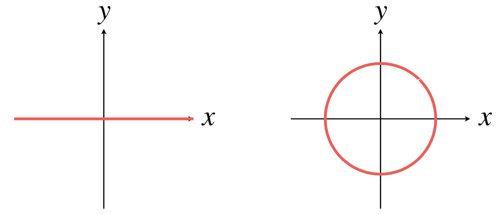
Figure 3.1: Location of the boundary on the constant time slice is depicted by the red line for the half holography (left) and the horizon-type holography (right).

Having said this, we consider holographic scenarios with a $(1+1)$-dimensional timelike boundary, which extends along the conformal time ($\eta$) direction and a spatial direction. At a constant time $\eta=\eta_{*}$, the boundary is specified by embedding of a one-dimensional curve into the $(r,\phi)$ plane. In this paper, we study the following two types of symmetric embedding (see also Fig. 3.1):

1. Half holography.

   The first type is motivated by the half de Sitter holography [27] and we place a boundary at a time $\eta=\eta_{*}$ on a straight line defined by

   $$y=0\quad{\rm with}\quad(x,y):=(r\cos\phi,r\sin\phi)\,,$$ (3.8)

   which cuts a constant-$\eta$ slice in half. We call this type the half holography in the following. Thanks to the translational invariance of the flat universe, the boundary enjoys a shift symmetry of $x$ and therefore the second derivative of the entanglement entropy can be used to test the (strong) subadditivity.

2. Horizon-type holography.

   The second type is motivated by the static patch holography [26] and we place a boundary at a time $\eta=\eta_{*}$ on a circle defined by

   $$r=\lambda|\eta_{*}|\,,\quad 0\leq\phi<2\pi\,.$$ (3.9)

   Here, we introduced a parameter $\lambda$ for later convenience. Especially for $\lambda=1$, the boundary coincides with the cosmological horizon. On the other hand, for $0<\lambda<1$ and $\lambda>1$, the boundary is located inside and outside of the horizon, respectively. We call this type the horizon-type holography in the following. Thanks to the rotational invariance of the flat universe, the boundary enjoys a shift symmetry of $\phi$ and therefore the second derivative of the entanglement entropy can be used to test the (strong) subadditivity.

Remarks on holography with a spacelike boundary.

As we mentioned, our analysis is applicable to holographic scenarios with a space-like boundary as well. For instance, suppose that the boundary is a spacelike surface defined by $\eta=\eta_{*}$, similarly to the dS/CFT correspondence [6]. If we identify the $y$ coordinate with a Euclidean time coordinate, the constant (Euclidean) time slice is the same as the half holography. Also, if we identify the radial coordinate $r$ with a Euclidean time, the constant time slice coincides with the one for the horizon-type holography. Since the holographic entanglement entropy depends only on the boundary points of the subsystem at a given time, the following analysis can be applied to these scenarios without any modification. The same remark applies to our analysis in open and closed universes of dS holography and the FLRW holography too.

3.2 Half holography

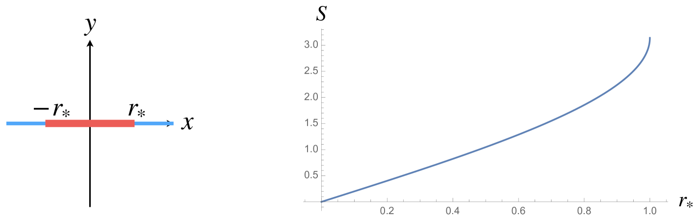
Figure 3.2: Left: Subsystem (red) and its complement (blue) in the half holography.
Right: Holographic entanglement entropy in the unit $4G=1$.

Now, we compute the holographic entanglement entropy for the half holography. We take a subsystem on an interval defined by

$$x\in(-r_{*},r_{*})\,,\quad y=0\,.$$ (3.10)

See also Fig. 3.2. Without loss of generality, we choose the conformal time as $\eta_{*}=-1$ for visual clarity, using the de Sitter dilatation symmetry. Then, the holographic entanglement entropy follows from Eq. (3.7) and the RT formula as

$$S=\frac{1}{2G}\arcsin r_{*}\,,$$ (3.11)

which is real as long as the subsystem interval fits inside the cosmological horizon, i.e., $r_{*}\leq 1$. However, it becomes complex once the interval goes beyond the event horizon $r_{*}>1$ [27]. Its second derivative with respect to (half of) the subsystem size $r_{*}$ reads

$$\frac{\partial^{2}S}{\partial r_{*}^{2}}=\frac{1}{2G}\frac{r_{*}}{(1-r_{*}^{2})^{\frac{3}{2}}}\,,$$ (3.12)

which is always positive as long as the subsystem interval is inside the event horizon. Hence, the half holography scenario is incompatible with the strong subadditivity. See also Fig. 3.2 for a plot of the holographic entanglement entropy and its second derivative.

3.3 Horizon-type holography

Next we study the horizon-type holography. We take a subsystem on an arc defined by

$$r=\lambda|\eta_{*}|\,,\quad\phi\in(0,\phi_{*})\,.$$ (3.13)

See also Fig. 3.3. Again, we choose $\eta_{*}=-1$ without loss of generality. Also, recall that $\lambda$ quantifies the boundary size compared to the horizon size. Then, the holographic entanglement entropy follows from Eq. (3.7) as

$$S=\frac{1}{4G}\arccos\left[1-2\lambda^{2}\sin^{2}\frac{\phi_{*}}{2}\right]\,,$$ (3.14)

which is real for all $\phi_{*}$ as long as the boundary is on or inside the horizon, i.e., $\lambda\leq 1$. In contrast, if the boundary is outside of the horizon $\lambda>1$, it becomes complex for $\sin\frac{\phi_{*}}{2}>\frac{1}{\lambda}$. On the other hand, the second derivative of the holographic entanglement entropy with respect to the subsystem size $\phi_{*}$ reads

$$\frac{\partial^{2}S}{\partial\phi_{*}^{2}}=-\frac{(1-\lambda^{2})}{8G}\frac{\lambda\sin\frac{\phi_{*}}{2}}{(1-\lambda^{2}\sin^{2}\frac{\phi_{*}}{2})^{\frac{3}{2}}}\,.$$ (3.15)

Interestingly, it is negative for all $\phi_{*}$ when the boundary is inside the cosmological horizon, whereas it is positive when the boundary is outside of the horizon. We conclude that the horizon-type holography is compatible with the strong subadditivity as long as the boundary is on or inside the horizon, at least within the scope of our current analysis. On the other hand, it is incompatible to put the boundary outside of the horizon. See also Fig. 3.3.

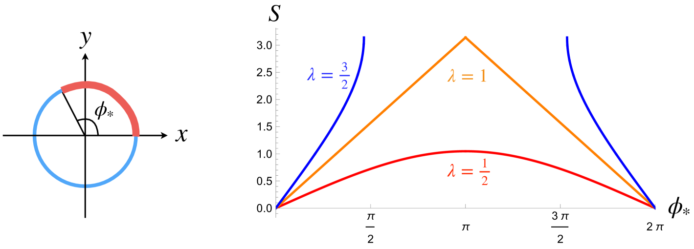
Figure 3.3: Left: Subsystem (red) and its complement (blue) in the horizon-type holography. Right: Holographic entanglement entropy for $\lambda=\frac{1}{2},1,\frac{3}{2}$ in the unit $4G=1$.

Before moving on to the closed and open universes, we comment on the $\lambda=1$ case, where the boundary is on the cosmological horizon. For this, the holographic entanglement entropy is simply proportional to the size of the subsystem or its complement:

$$S=\left\{\begin{array}[]{cl}\displaystyle\frac{\phi_{*}}{4G}&(0<\phi_{*}<\pi)\,,\\[8.53581pt] \displaystyle\frac{2\pi-\phi_{*}}{4G}&(\pi<\phi_{*}<2\pi)\,.\end{array}\right.$$ (3.18)

Hence, its second derivative vanishes except for $\phi_{*}=\pi$. It is suggestive that when the cosmological horizon is identified with the boundary, the negativity bound on the second derivative is saturated by the de Sitter spacetime, which also saturates the null energy condition. This motivates us to perform a similar analysis for more general FLRW universes and study the role of the null energy condition in this context.

4 FLRW holography

In this section we extend the previous analysis in the de Sitter space to general FLRW universes. In Sec. 4.1-Sec. 4.3 we perform an analytic study of the holographic entanglement entropy in the flat universe filled with an ideal fluid of constant equation of state. In Sec. 4.4, we conclude the analysis by discussing the location of the holographic boundary that accommodates a standard quantum field theory dual satisfying the strong subadditivity. See also Appendix B for the analysis of the closed and open universes.

4.1 Cosmological setup

Generality.

Consider a flat FLRW universe in three dimensions:

$$ds^{2}=a(\eta)^{2}\left[-d\eta^{2}+dr^{2}+r^{2}d\phi^{2}\right]\qquad(0\leq r<\infty\,,\,\,0\leq\phi<2\pi)\,,$$ (4.1)

where the scale factor $a(\eta)$ is kept arbitrary for this moment. In the following analysis of the holographic entanglement entropy, we need to evaluate the geodesic distance between two points $A,B$ on the same constant-$\eta$ slice $\eta=\eta_{*}$:

$$(\eta,r,\phi)=(\eta_{*},r_{A},\phi_{A}),\,\,(\eta_{*},r_{B},\phi_{B})\,.$$ (4.2)

For this purpose, it is convenient to use the translation and rotation symmetries of the flat slice $\eta=\eta_{*}$ to map the two points to

$$(\eta,r,\phi)=(\eta_{*},\tilde{r},0)\,,\,\,(\eta_{*},\tilde{r},\pi)\quad{\rm with}\quad\tilde{r}=\frac{1}{2}\sqrt{r_{A}^{2}+r_{B}^{2}-2r_{A}r_{B}\cos(\phi_{A}-\phi_{B})}\,,$$ (4.3)

or equivalently in the Euclidean coordinates $(x,y)=(r\cos\theta,r\sin\theta)$ as

$$(\eta,x,y)=(\eta_{*},\tilde{r},0)\,,\,\,(\eta_{*},-\tilde{r},0)\,.$$ (4.4)

The symmetry of the problem implies that $y=0$ along the geodesic, so that the geodesic is characterized by the conformal time $\eta(x)$ as a function of $x$. Then, the geodesic connecting the two points (4.4) is determined by minimization of the distance,

$$D(\eta_{*},\tilde{r})=\int_{-\tilde{r}}^{\tilde{r}}dx\,a\big{(}\eta(x)\big{)}\sqrt{1-\eta^{\prime}(x)^{2}}=2\int_{0}^{\tilde{r}}dx\,a\big{(}\eta(x)\big{)}\sqrt{1-\eta^{\prime}(x)^{2}}\,,$$ (4.5)

under the boundary conditions $\eta^{\prime}(0)=0$ and $\eta(\tilde{r})=\eta_{*}$, where we used the $Z_{2}$ symmetry $\eta(-x)=\eta(x)$ that follows from the boundary conditions $\eta(\pm\tilde{r})=\eta_{*}$.

Also, the translational symmetry along the $x$-axis implies the following conservation law:

$$\frac{a\big{(}\eta(x)\big{)}}{\sqrt{1-\eta^{\prime}(x)^{2}}}=a\big{(}\eta_{0}\big{)}\,,$$ (4.6)

where $\eta_{0}:=\eta(0)$ is the conformal time at the turning point of the geodesic. This implies $a(\eta(x))\leq a(\eta_{0})$. In particular, $\eta_{0}>\eta_{*}$ if the universe is in the expansion phase at $\eta=\eta_{*}$, which we assume in the following without loss of generality. Then, the geodesic is given by

$$x(\eta)=\pm\int^{\eta_{0}}_{\eta}\frac{d\tilde{\eta}}{\sqrt{1-\frac{a(\tilde{\eta})^{2}}{a(\eta_{0})^{2}}}}\,,\quad\tilde{r}=|x(\eta_{*})|=\int^{\eta_{0}}_{\eta_{*}}\frac{d\tilde{\eta}}{\sqrt{1-\frac{a(\tilde{\eta})^{2}}{a(\eta_{0})^{2}}}}\,,$$ (4.7)

where each of the $\pm$ sign describes a half of the geodesics. See also Figs. 4.1-4.3 for concrete profiles of geodesics. Correspondingly, the geodesic distance reads

$$D(\eta_{*},\tilde{r})=2\int^{\eta_{0}}_{\eta_{*}}d\eta\frac{a(\eta)^{2}}{\sqrt{a(\eta_{0})^{2}-a(\eta)^{2}}}\,.$$ (4.8)

The holographic entanglement entropy is obtained by dividing the geodesic distance by $4G$. Our task is now to perform the integrals (4.7)-(4.8).

Analytic results for constant $w$.

To be concrete, let us suppose that the universe is filled with an ideal fluid with a constant equation of state $w=p/\varepsilon$, where $\varepsilon>0$ and $p$ are the energy density and the pressure of the fluid, respectively. Then, the scale factor $a(\eta)$ enjoys a simple power law (see also Appendix A for basics of the FLRW universe):

$$a(\eta)=(w\eta)^{\frac{1}{w}}\,.$$ (4.9)

Here, we chose an expanding universe without loss of generality, so that the conformal time $\eta$ is in the range $0<\eta<\infty$ for the decelerating universe $w>0$ and $-\infty<\eta<0$ for the accelerating universe $w<0$, respectively. For the power-law scale factor (4.9), the integrals (4.7)-(4.8) can be performed analytically:

$$x(\eta) =\pm\left[\eta_{0}\cdot\frac{\sqrt{\pi}\,\Gamma\left[\frac{w+2}{2}\right]}{\Gamma\left[\frac{w+1}{2}\right]}-\eta\cdot{}_{2}F_{1}\left[\frac{1}{2},\frac{w}{2};\frac{w+2}{2};\left(\frac{\eta}{\eta_{0}}\right)^{\frac{2}{w}}\right]\right]\,,$$

$$\tilde{r} =\eta_{0}\cdot\frac{\sqrt{\pi}\,\Gamma\left[\frac{w+2}{2}\right]}{\Gamma\left[\frac{w+1}{2}\right]}-\eta_{*}\cdot{}_{2}F_{1}\left[\frac{1}{2},\frac{w}{2};\frac{w+2}{2};\left(\frac{\eta_{*}}{\eta_{0}}\right)^{\frac{2}{w}}\right]\,,$$ (4.10)

$$D(\eta_{*},\tilde{r}) =(w\eta_{0})^{1+\frac{1}{w}}\frac{\sqrt{\pi}\,\Gamma\left[\frac{w+2}{2}\right]}{\Gamma\left[\frac{w+3}{2}\right]}-\frac{2}{w+2}\frac{(w\eta_{*})^{1+\frac{2}{w}}}{(w\eta_{0})^{\frac{1}{w}}}{}_{2}F_{1}\left[\frac{1}{2},\frac{w+2}{2},\frac{w+4}{2},\left(\frac{\eta_{*}}{\eta_{0}}\right)^{\frac{2}{w}}\right]\,,$$

where each of the $\pm$ sign describes a half of the geodesics as we mentioned. Note that the above expression has an apparent singularity at $w=-2$, but they are finite even in this limit. For instance, an explicit form of $\tilde{r}$ and $d(\eta_{*},\tilde{r})$ for $w=-2$ is given by

$$\tilde{r}=-\eta_{*}\sqrt{1-\frac{\eta_{0}}{\eta_{*}}}-\frac{\eta_{0}}{2}\ln\frac{1+\sqrt{1-\frac{\eta_{0}}{\eta_{*}}}}{1-\sqrt{1-\frac{\eta_{0}}{\eta_{*}}}}\,,\quad d(\eta_{*},\tilde{r}) =\sqrt{-2\eta_{0}}\ln\frac{1+\sqrt{1-\frac{\eta_{0}}{\eta_{*}}}}{1-\sqrt{1-\frac{\eta_{0}}{\eta_{*}}}}\,.$$ (4.11)

Also note that thanks to the power-law nature (4.9) of the scale factor, $\eta_{*}$-dependence of the geodesic length enjoys a simple power-law,

$$D(\eta_{*},\tilde{r})=|\eta_{*}|^{1+\frac{1}{w}}D\left(\pm 1,\frac{\tilde{r}}{|\eta_{*}|}\right)\,,$$ (4.12)

where the plus and minus signs are for the decelerating universe ($w>0$) and the accelerating universe ($w<0$), respectively.

4.2 Half holography

First, we apply the analytic results (4.10) for the flat universe with constant $w$ to the half holography. Similarly to the de Sitter case, we put the boundary at a time $\eta=\eta_{*}$ on the straight line $y=0$ and take a subsystem on the interval,

$$x\in(-r_{*},r_{*})\,,\quad y=0\,.$$ (4.13)

Then, the holographic entanglement entropy reads

$$S=\frac{D(\eta_{*},r_{*})}{4G}\,.$$ (4.14)

Its $\eta_{*}$-dependence is a simple power-law (see Eq.(4.12))), which can be absorbed by an overall rescaling of the scale factor, so that we take $\eta_{*}=\pm 1$ without loss of generality. In the following we present the results for $w>0$, $-1<w<0$, and $w<-1$ in order.

Figure 4.1: Left: Profiles of geodesics for $w=\frac{1}{2}$. Red, orange, and blue curves are for $\eta_{0}=4,8,16$, respectively. The dashed line shows the $\eta_{*}=1$ slice, on which the subsystem is taken. Right: Holographic entanglement entropy for $w=\frac{1}{2},1,\frac{3}{2}$ in the unit $4G=1$. For visual clarity, $S/w^{1+\frac{1}{w}}$ is plotted in the figure.

Decelerating universe $(w>0)$.

First, typical profiles of geodesics in the decelerating universe $(w>0)$ are shown in the left panel of Fig. 4.1, which shows that for any $r_{*}$ there exists a single spacelike geodesic connecting the two boundary points. Indeed, one can confirm from Eq. (4.10) that the subsystem size $r_{*}$ is a monotonic function of the turning time $\eta_{0}$ with an asymptotic behavior,

$$r_{*}\simeq\eta_{0}\cdot\frac{\sqrt{\pi}\,\Gamma\left[\frac{w+2}{2}\right]}{\Gamma\left[\frac{w+1}{2}\right]}\quad(\eta_{0}\gg\eta_{*})\,.$$ (4.15)

Second, as shown in the right panel of Fig. 4.1, the holographic entanglement entropy is a convex function of the system size $r_{*}$. Hence, the half holography is incompatible with the strong subadditivity, similarly to the de Sitter case.

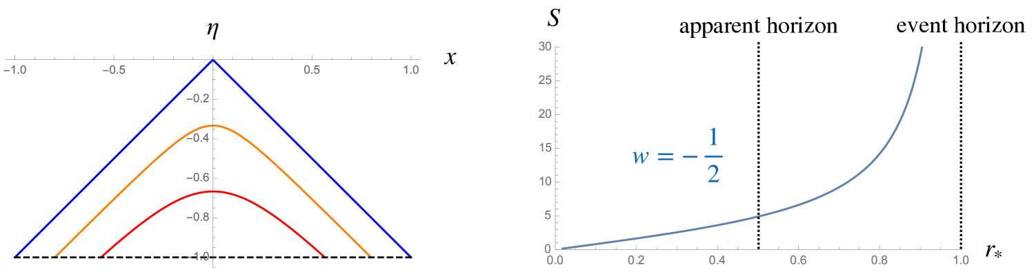
Figure 4.2: Left: Profiles of geodesics for $w=-\frac{1}{2}$. Red, orange, and blue curves are for $\eta_{0}=-\frac{3}{4},-\frac{1}{2},0$, respectively. The dashed line shows the $\eta_{*}=-1$ slice, on which the subsystem is taken. Right: Holographic entanglement entropy for $w=-\frac{1}{2}$ in the unit $4G=1$. The entropy diverges when the subsystem touches the event horizon, whereas nothing special happens at the apparent horizon.

Accelerating universe with $-1<w<0$.

Next, we consider the accelerating universe that satisfies the null energy condition, i.e., $-1<w<0$, for which the apparent horizon $r=w\eta$ is inside the event horizon $r=-\eta$ of an observer sitting at the origin $r=0$. In particular, at $\eta=\eta_{*}=-1$, they are located at $r=|w|$ and $r=1$, respectively. As depicted in the left panel of Fig. 4.2, there exists a spacelike geodesic connecting the two boundary points only when the subsystem is inside the event horizon $r_{*}<1$. Accordingly, the holographic entanglement entropy is no more real when the subsystem stretches outside the event horizon. This is similar to the de Sitter case. Second, as shown in the right panel of Fig. 4.2, the holographic entanglement entropy is a convex function of the system size $r_{*}$. Hence, the half holography is again incompatible with the strong subadditivity. Note that the holographic entanglement entropy diverges when the subsystem touches the event horizon, in contrast to the de Sitter case. Indeed, one can confirm the asymptotic behavior $S\propto(1-r_{*})^{1+\frac{1}{w}}$ in the limit $r_{*}\to 1$, using the analytic formulae (4.10).

Accelerating universe with $w<-1$.

Finally, we consider the accelerating universe that violates the null energy condition, i.e., $w<-1$, for which the apparent horizon $r=w\eta$ is outside of the event horizon $r=-\eta$ of an observer sitting at the origin $r=0$. The left panel of Fig. 4.3 illustrates the subsystem size $r_{*}$ as a function of the turning time $\eta_{0}$, which shows that there exists a spacelike geodesic connecting the two boundary points, even when the subsystem stretches outside the event horizon $r=1$. More remarkably, there exist two spacelike geodesics when $r_{*}$ is in the range $1\leq r_{*}<r_{\rm max}$, where $r_{\rm max}$ is the maximum subsystem size that accommodates a spacelike geodesic. These properties are in sharp contrast to the accelerating universe satisfying the null energy condition $-1\leq w<0$. See also the right panel of Fig. 4.3 for typical profiles of geodesics.

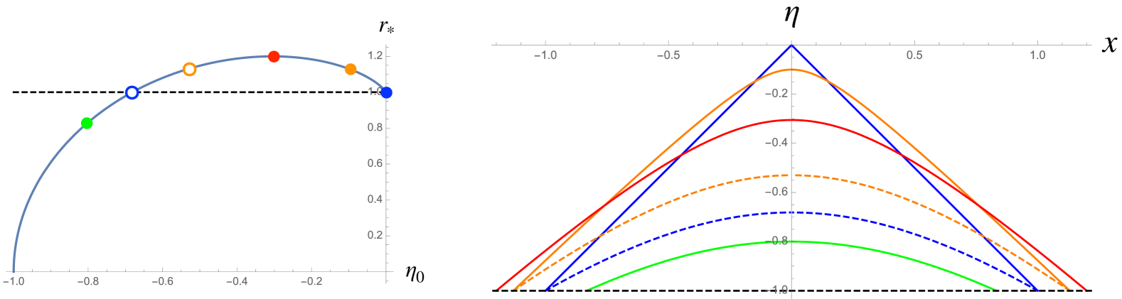
Figure 4.3: Left: Subsystem size $r_{*}$ as a function of turning time $\eta_{0}$ for $w=-2$. The dashed line shows the event horizon size $r_{*}=1$. The colored and white circles correspond to the solid and dashed curves of the same color in the right panel, respectively.
Right: Profiles of geodesics for $w=-2$. The solid and doted curves in the same color have the same subsystem size $r_{*}$, and the solid one has a shorter geodesic length. Red, orange, blue and green are for $r_{*}\simeq 1.20,1.13,1.00,0.83$, respectively.

Accordingly, the holographic entanglement entropy enjoys a peculiar phase transition at the event horizon scale $r_{*}=1$. See Fig. 4.4. When the subsystem fits inside the event horizon $r_{*}<1$, there exists a single geodesic for each $r_{*}$. In this regime, the holographic entanglement entropy is a convex function of $r_{*}$. At $r_{*}=1$, there appears a new branch represented by the solid curve in the regime $r_{*}\geq 1$ of the figure, which has a shorter geodesic length than the original branch (the dotted curve) and therefore it is identified with the Ryu–Takayanagi geodesic. Note that the entropy is a concave function of $r_{*}$ in the regime $1\leq r_{*}\leq r_{\rm max}$ ($r_{\rm max}\simeq 1.20$ for $w=-2$ used in the figure). For $r_{*}>r_{\rm max}$, there is no spacelike geodesic connecting the two boundary points, so that the entropy is no more real. Obviously, the holographic entanglement entropy does not satisfy the strong subadditivity and hence the half holography is incompatible similarly to the previous examples. Since the null energy condition is violated, there may be a real valued length geodesic even outside the event horizon.

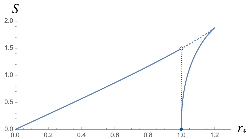
Figure 4.4: Holographic entanglement entropy for $w=-2$ as a function of subsystem size $r_{*}$.

4.3 Horizon-type holography

Next, we study the horizon-type holography. Similarly to the de Sitter case, we put the boundary at a time $\eta=\eta_{*}$ on the circle defined by

$$r=\lambda r_{\rm H}\,,\quad 0\leq\phi<2\pi\,,$$ (4.16)

where $r_{H}:=\frac{a(\eta_{*})}{a^{\prime}(\eta_{*})}$ is the radius of the apparent horizon and $\lambda$ quantifies the boundary size compared to it. Note that $r_{H}=w\eta_{*}$ for the power-law scale factor (4.9). Also, we take a subsystem on the arc,

$$r=\lambda r_{\rm H}\,,\quad\phi\in(0,\phi_{*})\,.$$ (4.17)

Then, $\tilde{r}$ in Eq. (4.3) is $\tilde{r}=\lambda r_{\rm H}\sin\frac{\phi_{*}}{2}$, so that the holographic entanglement entropy reads

$$S=\frac{D(\eta_{*},\lambda r_{\rm H}\sin\frac{\phi_{*}}{2})}{4G}\,.$$ (4.18)

In the following, we take $\eta_{*}=\pm 1$ without loss of generality and present the results for $w>0$ and $w<0$ in order.

Decelerating universe.

Fig. 4.5 illustrates the holographic entanglement entropy for $w=\frac{1}{2}$ as a function of the subsystem size $\phi_{*}$, whose properties are summarized as follows: First, for any $w>0$, the entropy has a real value for all $\phi_{*}$. Second, it is concave when the subsystem is large enough. This is due to the $Z_{2}$ symmetry $\phi_{*}\to 2\pi-\phi_{*}$ and the fact that the entropy takes a real value for all $\tilde{r}$. However, if the boundary is outside the apparent horizon $\lambda>1$, the entropy becomes convex in the small $\phi_{*}$ regime (see Sec. 4.4.1 for an analytic study). Hence, the horizon-type holography is compatible with the strong subadditivity only when the holographic boundary is on or inside the apparent horizon.

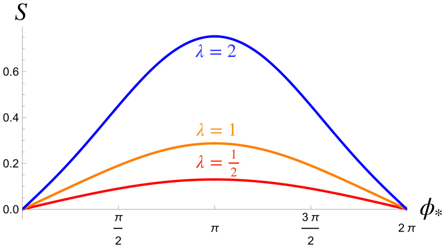
Figure 4.5: Holographic entanglement entropy for $w=\frac{1}{2}$ as a function of $\phi_{*}$. The boundary size is set as $\lambda=\frac{1}{2},1,2$, respectively.

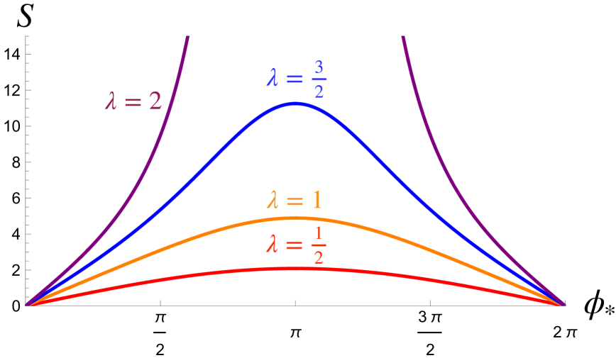
Figure 4.6: Holographic entanglement entropy for $w=-\frac{1}{2}$ as a function of $\phi_{*}$. The boundary size is set as $\lambda=\frac{1}{2},1,\frac{3}{2},2$, respectively.

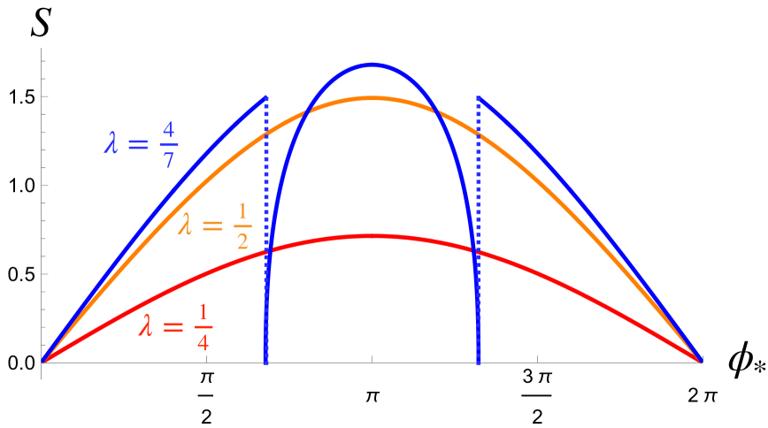
Figure 4.7: Holographic entanglement entropy for $w=-2$ as a function of $\phi_{*}$. The boundary size is set as $\lambda=\frac{1}{4},\frac{1}{2},\frac{4}{7}$, respectively.

Accelerating universe.

For the accelerating universe, the event horizon also comes into the game. For $-1\leq w<0$, the holographic entanglement entropy has a real value only when the subsystem fits inside the event horizon. Therefore, the condition for the entropy to be real for all $\phi_{*}$ reads $\lambda\leq|w|^{-1}$. The entropy for $w=-\frac{1}{2}$ as a function of $\phi_{*}$ is plotted in Fig. 4.6. There we find that the entropy is concave and the horizon-type holography is compatible with the strong subadditivity only when the holographic boundary is on or inside the apparent horizon (see also Sec. 4.4.1). On the other hand, for $w<-1$, the entanglement entropy enjoys a peculiar phase transition when the holographic boundary is outside the event horizon $\lambda>|w|^{-1}$. See Fig. 4.7. This may also be related with a violation of the null energy condition. Similarly to the half holography case, this makes the horizon-type holography with $\lambda>|w|^{-1}$ incompatible with the strong subadditivity. In contrast, if the holographic boundary is on or inside the event horizon $\lambda\leq|w|^{-1}$, the entanglement entropy is concave and compatible with the strong subadditivity.

4.4 Where can we place the holographic boundary?

To summarize so far, we have found for the flat FLRW universe with a power-law scale factor that the half holography is incompatible with the strong subadditivity, whereas compatibility of the horizon-type holography depends on the boundary size $\lambda$ as well as the equation of state $w$. The necessary conditions for the strong subadditivity to be satisfied in the horizon-type holography can be characterized by the subsystem size as follows:

1. Small subsystem

   The strong subadditivity is satisfied in the small subsystem regime $\phi_{*}\ll 1$, only when the holographic boundary is on or inside the apparent horizon $\lambda\leq 1$. This statement about small subsystems does not depend on the equation of state $w$ and applies to both accelerating and decelerating universes, essentially because local properties are insensitive to details of the cosmic history. Indeed, we show below analytically that this statement holds in general FLRW spacetimes, beyond the flat universe with a constant $w$. Also, note that the apparent horizon is defined locally, which is why its effects appear in the short-distance behavior of the holographic entanglement entropy.

2. Large subsystem

   On the other hand, the long-distance behavior is sensitive to the event horizon, which is defined based on global causal structure of the spacetime. Its impact on the horizon-type holography is distinct, especially when the event horizon of the accelerating universe is inside the apparent horizon, i.e., $w<-1$: If the holographic boundary is outside the event horizon, the holographic entanglement entropy experiences a peculiar phase transition, due to which the strong subadditivity is violated. Thus, we arrive at a necessary condition for the strong subadditivity: the holographic boundary in the accelerating universe has to be on or inside the event horizon.

   It is also interesting to rephrase our finding as follows: If the holographic boundary is put on the apparent horizon, the strong subadditivity is satisfied only when the universe satisfies the null energy condition $w\geq-1$. This is reminiscent of earlier works [55, 56, 57] that found a similar relation between the null energy condition and consistency of the holographic entanglement entropy in other spacetimes.

This observation leads to the following general expectation on the FLRW holography: If we require that the dual theory is an ordinary quantum field theory that respects unitarity and locality, the holographic boundary has to fit inside the apparent horizon and the event horizon of a geodesic observer. In particular, if we focus on a symmetric embedding of the holographic boundary into the FLRW universe, a natural holographic scenario is the horizon-type holography with $\lambda\leq 1$. To support this claim, in Sec. 4.4.1, we study the short-distance behavior of the holographic entanglement entropy in general FLRW universes.

Before moving on to this, we briefly comment on the original dS/CFT correspondence and possible extensions to the FLRW universe. As we remarked at the end of Sec. 3.1, our analysis can be applied directly to holography with a spacelike boundary at a constant time $\eta$. In particular, if we identify the $y$ coordinate with a Euclidean time coordinate of the would-be dual theory, the entanglement entropy is identical to the one we studied in the half holography. Since the strong subadditivity is always violated in this case, the would-be dual theory is a non-standard one. Indeed, it is expected to be non-unitary since the bulk and boundary do not share the notion of time. While it is interesting to explore such a holography with a non-standard dual theory, our take in this paper is in a different style: we are exploring a criteria for holographic and cosmological scenarios by postulating that the dual quantum field theory is well behaved.

4.4.1 Short-distance behavior in general FLRW universe.

To conclude this section, we make an analytic study of the short-distance behavior of the holographic entanglement entropy in general FLRW universes. Note that the long-distance behavior depends on the entire cosmic history and so it is hard to make a general study in contrast.

Consider a general flat FLRW universe and recall the general formulae (4.5)-(4.6) of the geodesic length. Combining them, the holographic entanglement entropy reads

$$S=\frac{1}{4G}\int_{-\tilde{r}}^{\tilde{r}}\frac{a^{2}(\eta(x))}{a(\eta(0))}dx\,,$$ (4.19)

where $\tilde{r}=r_{*}$ in the half holography and $\tilde{r}_{*}=\lambda r_{\rm H}\sin\frac{\phi_{*}}{2}$ in the horizon-type holography. Its small $\tilde{r}$ behavior reads

$$S=\frac{1}{4G}\left[2a(\eta_{*})\tilde{r}-\frac{1}{3}a^{\prime}(\eta_{*})\eta^{\prime\prime}(\tilde{r})\,\tilde{r}^{3}+\mathcal{O}(\tilde{r}^{5})\right]\,,$$ (4.20)

where we used the boundary condition $\eta^{\prime}(0)=0$ of the problem. On the other hand, the equation of motion that follows from Eq. (4.5) implies

$$\eta^{\prime\prime}(\tilde{r})=-\frac{a^{\prime}(\eta_{*})}{a(\eta_{*})}=-\frac{1}{r_{\rm H}}\,.$$ (4.21)

Then, we find

$$S=\frac{a_{*}}{4G}\left[2\tilde{r}+\frac{1}{3}\frac{\tilde{r}^{3}}{r_{\rm H}^{2}}+\mathcal{O}(\tilde{r}^{5})\right]\,.$$ (4.22)

In the half holography, we have $\tilde{r}=r_{*}$ with $r_{*}$ being a half of the subsystem size, hence the entropy is convex for any flat FLRW universe in the short-distance regime. In Appendix B, we find similar results for closed and open universes as well, hence we conclude that the half holography is incompatible with the strong subadditivity for any FLRW universe.

On the other hand, in the horizon-type holography, we have $\tilde{r}=\lambda r_{\rm H}\sin\frac{\phi_{*}}{2}$, where $\lambda$ is the size of the holographic boundary compared to the apparent horizon size and $\phi_{*}$ is the subsystem size. Substituting this to Eq. (4.22) gives the small $\phi_{*}$ expansion:

$$S=\frac{\lambda a_{*}r_{\rm H}}{4G}\left[\phi_{*}-\frac{1}{24}\left(1-\lambda^{2}\right)\phi_{*}^{3}+\mathcal{O}(\phi_{*}^{5})\right]\,.$$ (4.23)

In Appendix B, we find the same results for closed and open universes too. We thus conclude that the horizon-type holography is compatible with the strong subadditivity only when the holographic boundary is on or inside the apparent horizon $\lambda\leq 1$, which supports our claim that the holographic boundary has to fit inside the apparent horizon in order to have a standard quantum field theory dual.

5 Comments on matter entropy

In our analysis, so far we have ignored contributions of the matter entropy to the holographic entanglement entropy. In this section, we argue that this approximation can be justified naturally as long as the fluid description of the matter that fills the universe works well.

For simplicity, let us assume that the subsystem is smaller than its complement (e.g., $0<\phi_{*}<\pi$ in the horizon-type holography). Then, the geometric contribution $S_{\rm geo}$, i.e., the length of the geodesic is estimated as

$$S_{\rm geo}\sim\frac{L}{G}\,,$$ (5.1)

in terms of the physical size $L$ of the subsystem (e.g., $L=\lambda r_{\rm H}\phi_{*}$ in the horizon-type holography). On the other hand, the matter contribution is given by the matter entropy in the region surrounded by the subsystem and the RT surface (here just a geodesic), so that it is estimated as

$$S_{\rm mat}\sim sL^{2},$$ (5.2)

with $s$ being the entropy density of the fluid. Therefore, the matter contribution is negligible at least as long as the subsystem size $L$ is sufficiently small:

$$L\ll L_{*}\quad{\rm with}\quad L_{*}\sim\frac{1}{Gs}\,.$$ (5.3)

First, as we showed in the previous section, the short-distance behavior of the holographic entanglement entropy was enough to conclude that the half holography and the horizon-type holography with $\lambda>1$ are incompatible with the strong subadditivity. Hence, for whatever value of the critical length $L_{*}$, this conclusion is not affected by the matter entropy simply because we can always choose $L$ to be much smaller than a given $L_{*}$.

Next, let us take a closer look at the critical length $L_{*}$ to clarify applicability of our analysis at a long-distance scale. For concreteness, let us consider a flat universe filled with an ideal fluid. Then, its entropy density follows from the standard thermodynamics as

$$s=\frac{\varepsilon+p}{T}\,,$$ (5.4)

where for simplicity we assumed that the fluid has a single component of the temperature $T$. If the equation of state $w=p/\varepsilon$ satisfies $w+1=\mathcal{O}(1)$, we have $s\sim\varepsilon/T$, so that the critical length reads

$$L_{*}\sim\frac{T}{G\varepsilon}\,.$$ (5.5)

On the other hand, the Einstein equation relates the energy density $\varepsilon$ to the spacetime curvature as $G\varepsilon\sim H^{2}$ in terms of the Hubble parameter $H$. Note that the physical size of the apparent horizon $R_{\rm H}=ar_{\rm H}$ is $R_{\rm H}=H^{-1}$. Now, the condition $L\ll L_{*}$ is rephrased as

$$\frac{L}{R_{\rm H}}\ll\frac{T}{H}\,.$$ (5.6)

We emphasize that the matter entropy is $\mathcal{O}(G^{-1})$, which is at the same order of the $G$-expansion as the geometric contribution. This is why the Newton constant $G$ does not appear in the condition (5.6). For instance, in the horizon-type holography with $\lambda=\mathcal{O}(1)$, we have $L_{*}/R_{\rm H}\lesssim 1$, so that the matter contribution is negligible as long as the fluid temperature is higher than the Hubble scale:

$$T\gg H\,,$$ (5.7)

which is naturally satisfied as long as the fluid temperature is well-defined in the local patch of the universe. We thus conclude that the matter entropy is negligible and our analysis is applicable at least in a wide range of cosmological scenarios.

As a caveat, it is worth mentioning that in real cosmology, there are multiple components of fluids that have different temperatures. Moreover, the dominant component of the entropy is not necessarily the same as the dominant component of the energy density, so that the above simple argument does not work. For example, in our universe, radiation such as the cosmic microwave and neutrino backgrounds is negligible in the current energy density, but it is an important source of entropy. Besides, dark matter halo and Bekenstein–Hawking entropy of black holes and cosmological event horizon are paid attention as candidates of the leading source of entropy in the universe [58, 59]. It is interesting to explore how the story changes in the case where the dominant source of matter entropy is negligible as a source of the energy density, leaving it for future work.

6 Conclusion

In this paper, we studied the Ryu–Takayanagi surface or the geodesic in the three-dim FLRW universe. We considered two types of holographic scenario called the half holography and the horizon-type holography in the bulk spacetime and defined a subsystem on a constant time slice. To examine possible location of boundaries, we utilized the strong subadditivity of the entanglement entropy. We found in general that the strong subadditivity can be satisfied only in the horizon-type holography and in addition the holographic boundary has to fit inside the apparent horizon. Also, for the universe filled with an ideal fluid of constant equation of state $w<-1$, the condition is sharpened as that the holographic boundary has to fit inside the event horizon instead. Thus, assuming the null energy condition or $w>-1$, a natural holographic scenario is the horizon-type holography with the holographic boundary placed on or inside the apparent horizon.

Appendix A Basics of FLRW universe

Here, we summarize the basics of the FLRW universe, including the closed and open universes.

Coordinates.

The FLRW universe in $(d+1)$ dimensions is described by the metric,

$$ds^{2} =a^{2}(\eta)\left[-d\eta^{2}+\frac{dr^{2}}{1-kr^{2}}+r^{2}d\Omega_{d-1}^{2}\right]\,,$$ (A.1)

where $k=0,1,-1$ for the flat, closed, and open universes, respectively, and $r$ corresponds to the comoving radius of $S^{d-1}$. In particular, $d\eta=d\Omega_{d-1}=0$ gives a great circle of the $d$-dimensional sphere and hyperboloid describing the closed and open universes. To manifest the symmetry of the great circle, it is convenient to introduce the coordinate $\rho$ such that

$$\text{flat}:r=\rho\,,\quad\text{closed}:r=\sin\rho\,,\quad\text{open}:r=\sinh\rho\,,$$ (A.2)

in terms of which the metric reads

$$ds^{2} =a^{2}(\eta)\left[-d\eta^{2}+d\rho^{2}+r^{2}(\rho)d\Omega_{d-1}^{2}\right]\,.$$ (A.3)

Note that $r\in[0,1]$ and $\rho\in[0,\pi]$ for the closed universe, whereas $r,\rho\in[0,\infty)$ for the flat and open universes. We use these two coordinate systems interchangeably.

Apparent horizon.

On the apparent horizon, the ingoing/outgoing light rays do not feel the expansion/contraction of the universe, respectively. This condition can be stated as

$$0=\frac{d}{d\eta}(ar)=r\frac{da}{d\eta}+a\frac{dr}{d\eta}=ra^{\prime}\mp a\sqrt{1-kr^{2}}\,,$$ (A.4)

where the minus and plus signs are for the ingoing light rays in the expanding phase of the universe and the outgoing light rays in the contraction phase, respectively. Then, the radius $r_{\rm H}(\eta)$ of the apparent horizon at the time $\eta$ reads

$$r_{\rm H}(\eta)=\frac{1}{\sqrt{\left(\frac{a^{\prime}(\eta)}{a(\eta)}\right)^{2}+k}}\,.$$ (A.5)

If we define the corresponding $\rho$ coordinate such that $r_{\rm H}=\rho_{\rm H}$ (flat), $r_{\rm H}=\sin\rho_{\rm H}$ (closed), and $r_{\rm H}=\sinh\rho_{\rm H}$ (open), we have

$$\text{flat}:\rho_{\rm H}=\frac{a}{|a^{\prime}|}\,,\quad\text{closed}:\sin\rho_{\rm H}=\frac{a}{|a^{\prime}|}\,,\quad\text{open}:\sinh\rho_{\rm H}=\frac{a}{|a^{\prime}|}\,.$$ (A.6)

Benchmark examples.

Finally, we consider the universe filled with an ideal fluid of the constant equation of state $w=p/\varepsilon$. From the Einstein equation, the scale factor reads

$$\text{flat}:a(\eta)=\left(\frac{\eta}{\gamma}\right)^{\gamma}\,,\quad\text{closed}:a(\eta)=\left(\sin\frac{\eta}{|\gamma|}\right)^{\gamma}\,,\quad\text{open}:a(\eta)=\left(\sinh\frac{\eta}{\gamma}\right)^{\gamma}\,,$$ (A.7)

where the parameter $\gamma=\frac{2}{d(1+w)-2}$ is the same as the one defined in Eq. (2.14). Also, for simplicity, we suppressed an overall dimensionful factor that characterizes the physical size of the universe, similarly to the flat universe case. For the flat and open universes, we chose the expansion phase without loss of generality, so that $0<\eta<\infty$ for the decelerating universe ($\gamma>0$) and $-\infty<\eta<0$ for the accelerating universe ($\gamma<0$). On the other hand, in the closed universe, the $\rho$ coordinate satisfies $\rho\in[0,\pi]$, and the domain of conformal time is $\eta\in[0,|\gamma|\pi]$. See the following tables for qualitative features of the closed universe:

1. Decelerating closed universe $\gamma>0,k=1$

   $\eta=0$	$0<\eta<\gamma{\pi}/{2}$	$\gamma{\pi}/{2}<\eta<\pi\gamma$	$\eta=\gamma\pi$
   Big Bang	expansion $\dot{a}>0$	contraction $\dot{a}<0$	Big Crunch

2. Accelerating closed universe $\gamma<0,k=1$

   $0<\eta<|\gamma|\pi/2$	$|\gamma|{\pi}/{2}<\eta<|\gamma|\pi$
   contraction $\dot{a}<0$	expansion $\dot{a}>0$

From Eqs. (A.5)-(A.6), the location of the apparent horizon follows in the $r$ coordinate as

$$\text{flat}:r_{\rm H}=\frac{\eta}{\gamma}\,,\quad\text{closed}:r_{\rm H}=\sin\frac{\eta}{|\gamma|}\,,\quad\text{open}:r_{\rm H}=\sinh\frac{\eta}{\gamma}\,,$$ (A.8)

or equivalently in the $\rho$ coordinate as

$$\text{flat}:\rho_{\rm H}=\frac{\eta}{\gamma}\,,\quad\text{closed}:\rho_{\rm H}=\left\{\begin{array}[]{cc}\dfrac{\eta}{|\gamma|}&(0<\eta\leq\frac{\pi}{2})\,,\\ \pi-\dfrac{\eta}{|\gamma|}&\,\,(\frac{\pi}{2}\leq\eta<\pi)\,,\end{array}\right.\quad\text{open}:\rho_{\rm H}=\frac{\eta}{\gamma}\,.$$ (A.11)

Appendix B Closed and open universes

In this appendix, we extend the analysis of the main text to the closed and open universes.

B.1 Geometry

Consider the general FLRW universe in three dimensions:

$$ds^{2}=a^{2}(\eta)\left[-d\eta^{2}+\frac{dr^{2}}{1-kr^{2}}+r^{2}d\phi^{2}\right]=a^{2}(\eta)\left[-d\eta^{2}+d\rho^{2}+r^{2}(\rho)d\phi^{2}\right]\,.$$ (B.1)

where $k=0,1,-1$ for the flat, closed, and open universes respectively. The relation between the coordinates $r,\rho$ is

$$\text{flat}:r=\rho\,,\quad\text{closed}:r=\sin\rho\,,\quad\text{open}:r=\sinh\rho\,.$$ (B.2)

Note that $r\in[0,1]$ and $\rho\in[0,\pi]$ for the closed universe, whereas $r,\rho\in[0,\infty)$ for the flat and open universes. As we see shortly, the $r$ coordinate is useful in the horizon-type holography, whereas the $\rho$ coordinate is useful in the half holography. The comoving horizon radius $r_{\rm H}$ is given by

$$r_{\rm H}(\eta)=\frac{1}{\sqrt{\left(\frac{a^{\prime}(\eta)}{a(\eta)}\right)^{2}+k}}\,.$$ (B.3)

The corresponding $\rho$ coordinate defined such that $r_{\rm H}=\rho_{\rm H}$ (flat), $r_{\rm H}=\sin\rho_{\rm H}$ (closed), and $r_{\rm H}=\sinh\rho_{\rm H}$ (open) reads

$$\text{flat}:\rho_{\rm H}=\frac{a}{|a^{\prime}|}\,,\quad\text{closed}:\sin\rho_{\rm H}=\frac{a}{|a^{\prime}|}\,,\quad\text{open}:\sinh\rho_{\rm H}=\frac{a}{|a^{\prime}|}\,.$$ (B.4)

See Appendix A for more details.

B.2 Geodesics in general FLRW universe

Similarly to the flat universe case, we are interested in the geodesic distance between two points $A,B$ on the same constant-$\eta$ slice $\eta=\eta_{*}$:

$$(\eta,\rho,\phi)=(\eta_{*},\rho_{A},\phi_{A}),\,\,(\eta_{*},\rho_{B},\phi_{B})\,.$$ (B.5)

Using isometry of the FLRW spacetime, i.e., homogeneity and isotropy of the spatial slice $\eta=\eta_{*}$, we may map the two boundary points to

$$(\eta,\rho,\phi)=(\eta_{*},\tilde{\rho},0),\,\,(\eta_{*},\tilde{\rho},\pi),$$ (B.6)

where $\tilde{\rho}$ is a half of the geodesic distance on the two-dimensional spatial slice $\eta=\eta_{*}$. Its concrete form reads

flat $$:\,\,\,\,\,\,\,\,\,\,\,\tilde{\rho}\,=\frac{1}{2}\sqrt{\rho_{A}^{2}+\rho_{B}^{2}-2\rho_{A}\rho_{B}\cos(\phi_{A}-\phi_{B})}\,,$$ (B.7)

closed $$:\,\,\,\sin\tilde{\rho}\,=\sqrt{\frac{1-\cos\rho_{A}\cos\rho_{B}-\sin\rho_{A}\sin\rho_{B}\cos(\phi_{A}-\phi_{B})}{2}}\,,$$ (B.8)

open $$:\,\sinh\tilde{\rho}=\sqrt{\frac{\cosh\rho_{A}\cosh\rho_{B}-1-\sinh\rho_{A}\sinh\rho_{B}\cos(\phi_{A}-\phi_{B})}{2}}\,.$$ (B.9)

The symmetry of the problem implies that $d\phi=0$ along the geodesic, so that the geodesic problem reduces to the one in the two-dimensional spacetime $ds^{2}=a^{2}(\eta)[-d\eta^{2}+d\rho^{2}]$, which is nothing but the one we studied for the flat universe. Recycling the results there (see around Eqs. (4.6)-(4.8)), we find the following formula of the geodesic length $D(\eta_{*},\tilde{\rho})$:

$$D(\eta_{*},\tilde{\rho})=2\int^{\eta_{0}}_{\eta_{*}}d\eta\frac{a(\eta)^{2}}{\sqrt{a(\eta_{0})^{2}-a(\eta)^{2}}}\quad{\rm wtih}\quad\tilde{\rho}=\int^{\eta_{0}}_{\eta_{*}}\frac{d\tilde{\eta}}{\sqrt{1-\frac{a(\tilde{\eta})^{2}}{a(\eta_{0})^{2}}}}\,,$$ (B.10)

where we assumed that the universe is in the expansion phase at $\eta=\eta_{*}$ and therefore the conformal time $\eta_{0}$ at the turning point of the geodesic satisfies $\eta_{0}>\eta_{*}$.

Short-distance behavior.

Similarly to the flat universe case, the short-distance behavior of the geodesic length (B.10) can be studied without specifying details of the cosmic history. First, by performing the small $\tilde{\rho}$ expansion and using the equation of motion and the boundary conditions (see discussion around Eqs. (4.20)-(4.21) for details), we find

$$D(\eta_{*},\tilde{\rho})=a(\eta_{*})\left[2\tilde{\rho}+\frac{1}{3}\left(\frac{a^{\prime}(\eta_{*})}{a(\eta_{*})}\right)^{2}\tilde{\rho}^{3}+\mathcal{O}(\tilde{\rho}^{5})\right]\,.$$ (B.11)

It is also convenient to rewrite it in terms of the $r$ coordinate defined by

$$\text{flat}:\tilde{r}=\tilde{\rho}\,,\quad\text{closed}:\tilde{r}=\sin\tilde{\rho}\,,\quad\text{open}:\tilde{r}=\sinh\tilde{\rho}\,,$$ (B.12)

as follows:

$$D(\eta_{*},\tilde{\rho})=a(\eta_{*})\left[2\tilde{r}+\frac{1}{3}\frac{\tilde{r}^{3}}{r_{\rm H}^{2}}+\mathcal{O}(\tilde{r}^{5})\right]\,,$$ (B.13)

where $r_{\rm H}$ is the radius of the apparent horizon at the time $\eta=\eta_{*}$, i.e., $r_{\rm H}=r_{\rm H}(\eta_{*})$ with Eq. (A.5). In the next subsection, we discuss the short-distance behavior of the holographic entanglement entropy based on Eq. (B.11) and Eq. (B.13).

B.3 Holographic scenarios

Similarly to the flat universe case, we consider the following two types of holographic scenarios. This subsection summarizes general properties of the holographic entanglement entropy, leaving concrete analysis in specific cosmological scenarios to the rest of the section.

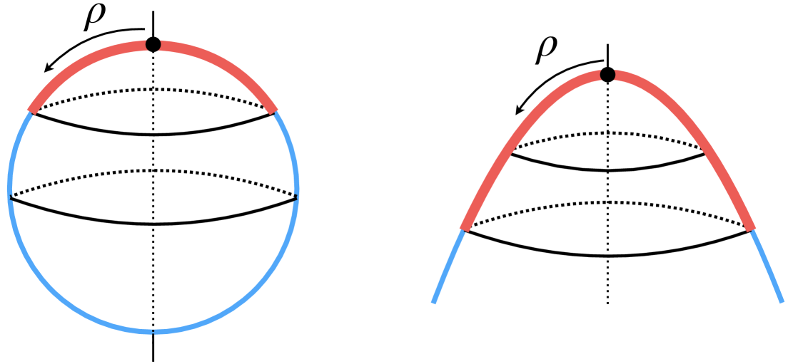
Figure B.1: The two-dimensional sphere (left) and hyperboloid (right) describe the closed and open universes at $\eta=\eta_{*}$. The black point is for the North pole $\rho=0$ and the rotation angle around the straight line is $\phi$. The subsystem and its complement in the half holography are depicted by the red and blue curves, respectively.

Half holography.

In the half holography, we place the holographic boundary at $\eta=\eta_{*}$ on a curve defined by $\rho\sin\phi=0$, which cuts the universe in half. Note that a shift symmetry on the holographic boundary is guaranteed by the isometry. As a subsystem, we take an interval defined by

$$\rho\cos\phi\in[-\rho_{*},\rho_{*}]\,,\quad\rho\sin\phi=0\,.$$ (B.14)

See also Fig. B.1. Then, the holographic entanglement entropy reads

$$S=\frac{D(\eta_{*},\rho_{*})}{4G}\,.$$ (B.15)

In particular, its short-distance behavior follows from Eq. (B.11) as

$$S=\frac{a(\eta_{*})}{4G}\left[2\tilde{\rho}+\frac{1}{3}\left(\frac{a^{\prime}(\eta_{*})}{a(\eta_{*})}\right)^{2}\tilde{\rho}^{3}+\mathcal{O}(\tilde{\rho}^{5})\right]\,,$$ (B.16)

which shows that the entropy is always convex in the short-distance regime. Therefore, we conclude that the half holography is incompatible with the strong subadditivity in the closed and open universes as well.

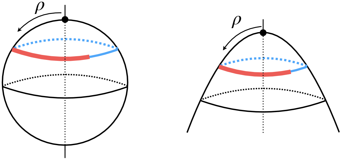
Figure B.2: The two-dimensional sphere (left) and hyperboloid (right) describe the closed and open universes at $\eta=\eta_{*}$. The subsystem and its complement in the horizon-type holography are depicted by the red and blue curves, respectively.

Horizon-type holography.

In the horizon-type holography, the apparent horizon plays an important role, whose radius $r_{\rm H}=r_{\rm H}(\eta_{*})$ at the time $\eta=\eta_{*}$ is given in Eq. (A.5). We place the holographic boundary on a circle defined in the $r$ coordinate as

$$r=\lambda r_{\rm H}$$ (B.17)

or equivalently in the $\rho$ coordinate as

$$\text{flat}:\rho=\lambda r_{\rm H}\,,\quad\text{closed}:\sin\rho=\lambda r_{\rm H}\,,\quad\text{open}:\sinh\rho=\lambda r_{\rm H}\,,$$ (B.18)

where $\lambda$ quantifies the size of the boundary compared to the apparent horizon. As a subsystem, we take an arc defined by

$$r=\lambda r_{\rm H}\,,\quad\phi\in[0,\phi_{*}]\,.$$ (B.19)

and similarly in the $\rho$ coordinate. See also Fig. B.2. The corresponding $\tilde{\rho}$ defined in Eqs. (B.7)-(B.9) reads

$$\text{flat}:\tilde{\rho}=\lambda r_{\rm H}\sin\frac{\phi_{*}}{2}\,,\quad\text{closed}:\sin\tilde{\rho}=\lambda r_{\rm H}\sin\frac{\phi_{*}}{2}\,,\quad\text{open}:\sinh\tilde{\rho}=\lambda r_{\rm H}\sin\frac{\phi_{*}}{2}\,.$$ (B.20)

Note that in terms of $\tilde{r}$ defined in Eq. (B.12), the above relations are summarized simply as

$$\tilde{r}=\lambda r_{\rm H}\sin\frac{\phi_{*}}{2}\,.$$ (B.21)

Then, the holographic entanglement entropy reads

flat $$:S=\frac{D(\eta_{*},\lambda r_{\rm H}\sin\frac{\phi_{*}}{2})}{4G}\,,$$ (B.22)

closed $$:S=\frac{D(\eta_{*},\arcsin[\lambda r_{\rm H}\sin\frac{\phi_{*}}{2}])}{4G}\,,$$ (B.23)

open $$:S=\frac{D(\eta_{*},\text{arsinh}[\lambda r_{\rm H}\sin\frac{\phi_{*}}{2}])}{4G}\,.$$ (B.24)

In particular, its short-distance behavior follows from Eq. (B.13) as

$$S=\frac{\lambda a_{*}r_{\rm H}}{4G}\left[\phi_{*}-\frac{1}{24}\left(1-\lambda^{2}\right)\phi_{*}^{3}+\mathcal{O}(\phi_{*}^{5})\right]\,.$$ (B.25)

Hence, in the short-distance regime, the horizon-type holography is compatible with strong subadditivity, only when the holographic boundary is on or inside the apparent horizon.

B.4 de Sitter spacetime

As a concrete example, we consider de Sitter spacetime, for which we can compute the holographic entanglement entropy analytically by performing the integral (B.10) or by using the embedding coordinate expression (3.3). Here, we present the latter analysis and show that qualitative features of the entropy do not depend on the curvature $k$ of the universe.

B.4.1 Coordinate systems

We first introduce the closed and open charts of de Sitter spacetime and derive an analytic formula for the geodesic length using the embedding language.

Closed universe.

The de Sitter closed universe is described by the coordinates,

$$X^{0}=-\frac{1}{\tan\eta},\quad X^{1}=\frac{\cos\rho}{\sin\eta},\quad X^{2}=\frac{\sin\rho}{\sin\eta}\cos\phi,\quad X^{3}=\frac{\sin\rho}{\sin\eta}\sin\phi$$ (B.26)

with

$$0<\eta<\pi\,,\quad 0\leq\rho\leq\pi\,,\quad 0\leq\phi<2\pi\,.$$ (B.27)

The corresponding metric is

$$ds^{2}=\frac{-d\eta^{2}+d\rho^{2}+\sin^{2}\rho\,d\phi^{2}}{\sin^{2}\eta}\,.$$ (B.28)

The cosmological event horizon for the observer sitting at $\rho=0$ is located at

$$\rho=\left\{\begin{array}[]{cc}\eta&(0<\eta\leq\frac{\pi}{2})\,,\\ \pi-\eta&(\frac{\pi}{2}\leq\eta<\pi)\,.\end{array}\right.$$ (B.31)

The geodesic distance $D$ of two points $(\eta_{A},\rho_{A},\phi_{A})$ and $(\eta_{B},\rho_{B},\phi_{B})$ reads

$$\cos D=1-\frac{\cos(\eta_{A}-\eta_{B})-\cos\rho_{A}\cos\rho_{B}-\sin\rho_{A}\sin\rho_{B}\cos(\phi_{A}-\phi_{B})}{\sin\eta_{A}\sin\eta_{B}}\,.$$ (B.32)

Open universe.

The de Sitter open universe is described by the coordinates,

$$X^{0}=-\frac{\cosh\rho}{\sinh\eta}\,,\quad X^{1}=\frac{1}{\tanh\eta}\,,\quad X^{2}=\frac{\sinh\rho}{\sinh\eta}\cos\phi\,,\quad X^{3}=\frac{\sinh\rho}{\sinh\eta}\sin\phi$$ (B.33)

with

$$-\infty<\eta<0\,,\quad 0\leq\rho<\infty\,,\quad 0\leq\phi<2\pi\,.$$ (B.34)

The corresponding metric is

$$ds^{2}=\frac{-d\eta^{2}+d\rho^{2}+\sinh^{2}\rho\,d\phi^{2}}{\sinh^{2}\eta}\,.$$ (B.35)

The cosmological event horizon for the observer sitting at $\rho=0$ is located at $\rho=-\eta$. The geodesic distance of two points $(\eta_{A},\rho_{A},\phi_{A})$ and $(\eta_{B},\rho_{B},\phi_{B})$ reads

$$\cos D=1-\frac{-\cosh(\eta_{A}-\eta_{B})+\cosh\rho_{A}\cosh\rho_{B}-\sinh\rho_{A}\sinh\rho_{B}\cos(\phi_{A}-\phi_{B})}{\sinh\eta\sinh\eta_{B}}\,.$$ (B.36)

B.4.2 Holographic entanglement entropy

Now, we compute the holographic entanglement entropy in the two holographic scenarios.

Half holography.

In the half holography, we take the subsystem at the time $\eta=\eta_{*}$ as

$$\rho\cos\phi\in[-\rho_{*},\rho_{*}]\,,\quad\rho\sin\phi\,.$$ (B.37)

Then, the holographic entanglement entropy $\displaystyle S=\frac{D}{4G}$ with $D$ being the geodesic distance of the two boundary points reads

$$\text{closed}:\,\,S=\frac{1}{2G}\arcsin\frac{\sin\rho_{*}}{\sin\eta_{*}}\,,\quad\text{open}:\,\,S=\frac{1}{2G}\arcsin\frac{\sinh\rho_{*}}{\sinh\eta_{*}}\,,$$ (B.38)

which is real as long as the subsystem interval is inside the horizon. More explicitly, we may rewrite it in terms of the $r$ coordinate, $r_{*}=\sin\rho_{*}$ (closed) and $r_{*}=\sinh\rho_{*}$ (open), and the horizon radius, $r_{\rm H}=\sin\eta_{*}$ (closed) and $r_{\rm H}=\sinh\eta_{*}$ (open), as

$$S=\frac{1}{2G}\arcsin\frac{r_{*}}{r_{\rm H}}\,.$$ (B.39)

This formula summarizes the results for all the flat, closed, and open universes. See also the flat universe result (3.11), where $r_{\rm H}=1$. On the other hand, the second derivative of the entropy with respect to (half of) the subsystem size $\rho_{*}$ is

closed $$:\,\,\frac{\partial^{2}S}{\partial\rho_{*}^{2}}=\frac{1}{2G}\frac{\cos^{2}\eta_{*}\sin\rho_{*}}{(\sin\eta_{*}^{2}-\sin\rho_{*}^{2})^{\frac{3}{2}}}\,,$$ (B.40)

open $$:\,\,\frac{\partial^{2}S}{\partial\rho_{*}^{2}}=\frac{1}{2G}\frac{\cosh^{2}\eta_{*}\sinh\rho_{*}}{(\sinh\eta_{*}^{2}-\sinh\rho_{*}^{2})^{\frac{3}{2}}}\,.$$ (B.41)

Similarly to the flat universe case, the second derivative is always positive, hence the half holography is incompatible with the strong subadditivity.

Horizon-type holography.

In the horizon-type holography, we take a subsystem at the time $\eta=\eta_{*}$ in the $r$ coordinate as

$$r=\lambda r_{\rm H}\,,\quad\phi\in[0,\phi_{*}]$$ (B.42)

or equivalently in the $\rho$ coordinate as

$$\text{closed}:\sin\rho=\lambda r_{\rm H}\,,\,\,\phi\in[0,\phi_{*}]\,,\quad\text{open}:\sinh\rho=\lambda r_{\rm H}\,,\,\,\phi\in[0,\phi_{*}]\,.$$ (B.43)

Note that the location of the holographic boundary and the choice of the subsystem are essentially the same as the flat universe case. As a result, the holographic entanglement entropy and its second derivative take the same form as before:

$$S=\frac{1}{2G}\arcsin\left[\lambda\sin\frac{\phi_{*}}{2}\right]\,,\quad\frac{\partial^{2}S}{\partial\phi_{*}^{2}}=-\frac{(1-\lambda^{2})}{8G}\frac{\lambda\sin\frac{\phi_{*}}{2}}{(1-\lambda^{2}\sin^{2}\frac{\phi_{*}}{2})^{\frac{3}{2}}}\,,$$ (B.44)

which are applicable for all the flat, closed, and open universes. We conclude also for the closed and open universes that the horizon-type holography is compatible with the strong subadditivity as long as the boundary is on or inside the horizon, at least within the scope of our current analysis.

B.5 FLRW universe with constant equation of state

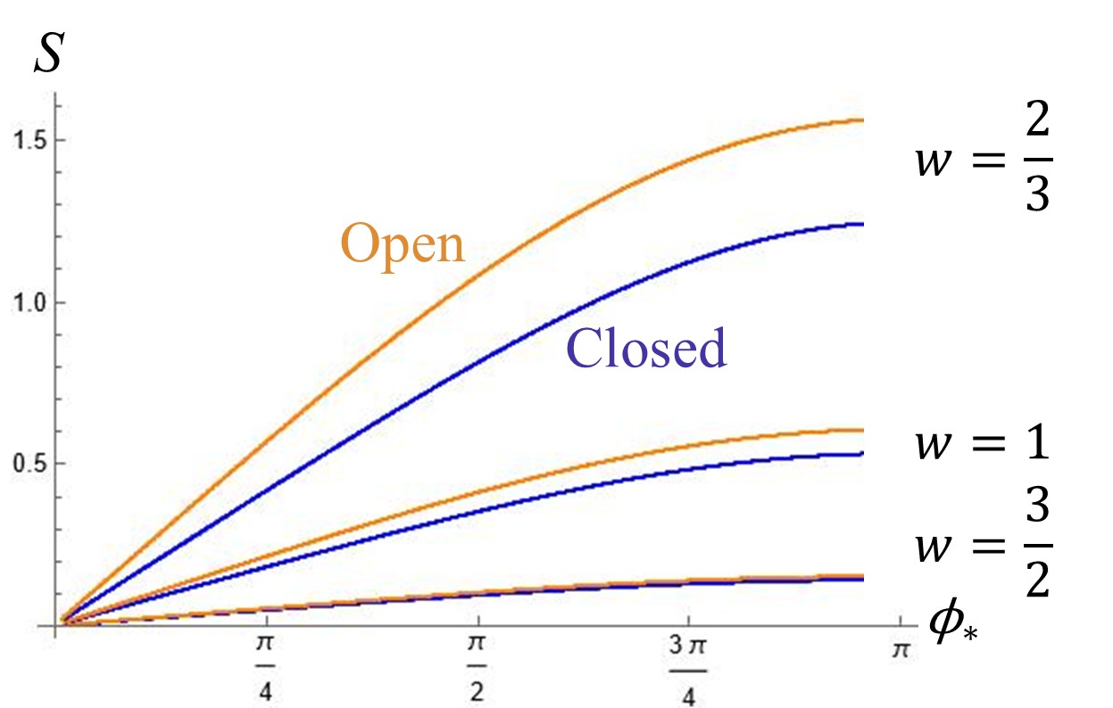
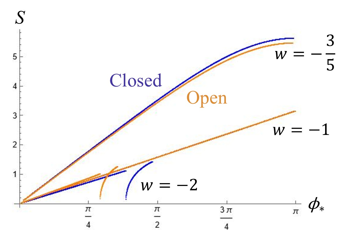
Figure B.3: The holographic entanglement entropy in open universe (orange) and closed universe (blue). We fix the boundary at the apparent horizon $\lambda=1$ at the time slice $\eta_{*}=0.5$ for the decelerating universes (left) and $\eta_{*}=-0.5$ for the accelerating universes (right), respectively. Note that the plots exclude $\phi_{*}\simeq 0,\pi$ due to numerical error.

Finally, we consider the closed and open universes $k=\pm 1$ filled with an ideal fluid of a constant equation of state parameter $w=p/\varepsilon$, where $\varepsilon>0$ and $p$ are the energy density and pressure of the fluid, respectively. Then, the scale factor $a(\eta)$ takes the form,

$$\text{closed}:a(\eta)=[\sin(w\eta)]^{\frac{1}{w}}\,,\quad\text{open}:a(\eta)=[\sinh(w\eta)]^{\frac{1}{w}}\,.$$ (B.45)

See also Eq. (A.7). Here, without loss of generality, we normalized the scale factor such that $a(\eta)=1$ when $\sin(w\eta)=1$ for the closed universe and $\sinh(w\eta)=1$ for the open universe, respectively. Also, $0<w\eta<\pi$ for the closed universe. For the open universe, we choose the expanding universe, so that $0<\eta<\infty$ for the decelerating universe $w>0$ and $-\infty<\eta<0$ for the accelerating universe. We can perform a similar computation to the main text by substituting the scale factor for (B.10). The numerical results for the horizon-type boundary are illustrated in Fig. B.3, which shows that the qualitative features of the holographic entanglement entropy do not depend on the curvature $k$ very much. The difference of the open and closed universe is their expansion rate (B.45). In the decelerating universe, the open universe is bigger when we take the same time and equation of state parameters, leading to a larger RT surface. The accelerating universe is the opposite, i.e., the closed universe has a larger universe size and the RT surface. As a special case, you can find in the figure that the holographic entanglement entropy in de Sitter spacetime $w=-1$ is the same for all $k$, which confirms the discussion in the previous subsection. Note that the results of the flat universe are in-between those of the open and closed universe.

References

- [1] J. M. Maldacena, The Large N limit of superconformal field theories and supergravity, Adv. Theor. Math. Phys. 2 (1998) 231–252, [hep-th/9711200].
- [2] S. Ryu and T. Takayanagi, Holographic derivation of entanglement entropy from AdS/CFT, Phys. Rev. Lett. 96 (2006) 181602, [hep-th/0603001].
- [3] S. Ryu and T. Takayanagi, Aspects of Holographic Entanglement Entropy, JHEP 08 (2006) 045, [hep-th/0605073].
- [4] J. D. Bekenstein, Black holes and entropy, Phys. Rev. D 7 (1973) 2333–2346.
- [5] S. W. Hawking, Particle Creation by Black Holes, Commun. Math. Phys. 43 (1975) 199–220. [Erratum: Commun.Math.Phys. 46, 206 (1976)].
- [6] A. Strominger, The dS / CFT correspondence, JHEP 10 (2001) 034, [hep-th/0106113].
- [7] A. A. Starobinsky, A New Type of Isotropic Cosmological Models Without Singularity, Phys. Lett. B 91 (1980) 99–102.
- [8] K. Sato, First Order Phase Transition of a Vacuum and Expansion of the Universe, Mon. Not. Roy. Astron. Soc. 195 (1981) 467–479.
- [9] A. H. Guth, The Inflationary Universe: A Possible Solution to the Horizon and Flatness Problems, Phys. Rev. D 23 (1981) 347–356.
- [10] A. D. Linde, A New Inflationary Universe Scenario: A Possible Solution of the Horizon, Flatness, Homogeneity, Isotropy and Primordial Monopole Problems, Phys. Lett. B 108 (1982) 389–393.
- [11] Planck Collaboration, Y. Akrami et al., Planck 2018 results. X. Constraints on inflation, Astron. Astrophys. 641 (2020) A10, [arXiv:1807.06211].
- [12] F. Larsen, J. P. van der Schaar, and R. G. Leigh, De Sitter holography and the cosmic microwave background, JHEP 04 (2002) 047, [hep-th/0202127].
- [13] J. M. Maldacena, Non-Gaussian features of primordial fluctuations in single field inflationary models, JHEP 05 (2003) 013, [astro-ph/0210603].
- [14] J. P. van der Schaar, Inflationary perturbations from deformed CFT, JHEP 01 (2004) 070, [hep-th/0307271].
- [15] D. Seery and J. E. Lidsey, Non-Gaussian Inflationary Perturbations from the dS/CFT Correspondence, JCAP 06 (2006) 001, [astro-ph/0604209].
- [16] A. Kehagias and A. Riotto, Operator Product Expansion of Inflationary Correlators and Conformal Symmetry of de Sitter, Nucl. Phys. B 864 (2012) 492–529, [arXiv:1205.1523].
- [17] A. Bzowski, P. McFadden, and K. Skenderis, Holography for inflation using conformal perturbation theory, JHEP 04 (2013) 047, [arXiv:1211.4550].
- [18] K. Schalm, G. Shiu, and T. van der Aalst, Consistency condition for inflation from (broken) conformal symmetry, JCAP 03 (2013) 005, [arXiv:1211.2157].
- [19] J. Garriga and Y. Urakawa, Inflation and deformation of conformal field theory, JCAP 07 (2013) 033, [arXiv:1303.5997].
- [20] D. Anninos, T. Anous, D. Z. Freedman, and G. Konstantinidis, Late-time Structure of the Bunch-Davies De Sitter Wavefunction, JCAP 11 (2015) 048, [arXiv:1406.5490].
- [21] A. Shukla, S. P. Trivedi, and V. Vishal, Symmetry constraints in inflation, -vacua, and the three point function, JHEP 12 (2016) 102, [arXiv:1607.08636].
- [22] N. Arkani-Hamed, D. Baumann, H. Lee, and G. L. Pimentel, The Cosmological Bootstrap: Inflationary Correlators from Symmetries and Singularities, JHEP 04 (2020) 105, [arXiv:1811.00024].
- [23] D. Baumann, C. Duaso Pueyo, A. Joyce, H. Lee, and G. L. Pimentel, The cosmological bootstrap: weight-shifting operators and scalar seeds, JHEP 12 (2020) 204, [arXiv:1910.14051].
- [24] D. Baumann, C. Duaso Pueyo, A. Joyce, H. Lee, and G. L. Pimentel, The Cosmological Bootstrap: Spinning Correlators from Symmetries and Factorization, SciPost Phys. 11 (2021) 071, [arXiv:2005.04234].
- [25] E. Pajer, D. Stefanyszyn, and J. Supeł, The Boostless Bootstrap: Amplitudes without Lorentz boosts, JHEP 12 (2020) 198, [arXiv:2007.00027]. [Erratum: JHEP 04, 023 (2022)].
- [26] L. Susskind, De Sitter Holography: Fluctuations, Anomalous Symmetry, and Wormholes, Universe 7 (2021), no. 12 464, [arXiv:2106.03964].
- [27] T. Kawamoto, S.-M. Ruan, Y.-k. Suzuki, and T. Takayanagi, A half de Sitter holography, JHEP 10 (2023) 137, [arXiv:2306.07575].
- [28] D. Anninos, D. A. Galante, and C. Maneerat, Cosmological observatories, Class. Quant. Grav. 41 (2024), no. 16 165009, [arXiv:2402.04305].
- [29] E. Silverstein, Black hole to cosmic horizon microstates in string/M theory: timelike boundaries and internal averaging, JHEP 05 (2023) 160, [arXiv:2212.00588].
- [30] G. Batra, G. B. De Luca, E. Silverstein, G. Torroba, and S. Yang, Bulk-local dS3 holography: the matter with + 2, JHEP 10 (2024) 072, [arXiv:2403.01040].
- [31] L. McGough, M. Mezei, and H. Verlinde, Moving the CFT into the bulk with , JHEP 04 (2018) 010, [arXiv:1611.03470].
- [32] M. Guica and R. Monten, and the mirage of a bulk cutoff, SciPost Phys. 10 (2021), no. 2 024, [arXiv:1906.11251].
- [33] A. Lewkowycz, J. Liu, E. Silverstein, and G. Torroba, and EE, with implications for (A)dS subregion encodings, JHEP 04 (2020) 152, [arXiv:1909.13808].
- [34] Y. Nomura, N. Salzetta, F. Sanches, and S. J. Weinberg, Spacetime Equals Entanglement, Phys. Lett. B 763 (2016) 370–374, [arXiv:1607.02508].
- [35] Y. Nomura, N. Salzetta, F. Sanches, and S. J. Weinberg, Toward a Holographic Theory for General Spacetimes, Phys. Rev. D 95 (2017), no. 8 086002, [arXiv:1611.02702].
- [36] V. Franken, H. Partouche, F. Rondeau, and N. Toumbas, Closed FRW holography: a time-dependent ER=EPR realization, JHEP 05 (2024) 219, [arXiv:2310.20652].
- [37] G. ’t Hooft, Dimensional reduction in quantum gravity, Conf. Proc. C 930308 (1993) 284–296, [gr-qc/9310026].
- [38] L. Susskind, The World as a hologram, J. Math. Phys. 36 (1995) 6377–6396, [hep-th/9409089].
- [39] O. Aharony, S. S. Gubser, J. M. Maldacena, H. Ooguri, and Y. Oz, Large N field theories, string theory and gravity, Phys. Rept. 323 (2000) 183–386, [hep-th/9905111].
- [40] S. S. Gubser, I. R. Klebanov, and A. M. Polyakov, Gauge theory correlators from noncritical string theory, Phys. Lett. B 428 (1998) 105–114, [hep-th/9802109].
- [41] E. Witten, Anti-de Sitter space and holography, Adv. Theor. Math. Phys. 2 (1998) 253–291, [hep-th/9802150].
- [42] T. Banks, M. R. Douglas, G. T. Horowitz, and E. J. Martinec, AdS dynamics from conformal field theory, hep-th/9808016.
- [43] K. Skenderis, Lecture notes on holographic renormalization, Class. Quant. Grav. 19 (2002) 5849–5876, [hep-th/0209067].
- [44] M. Bianchi, D. Z. Freedman, and K. Skenderis, Holographic renormalization, Nucl. Phys. B 631 (2002) 159–194, [hep-th/0112119].
- [45] A. B. Zamolodchikov, Expectation value of composite field T anti-T in two-dimensional quantum field theory, hep-th/0401146.
- [46] S. Kachru, R. Kallosh, A. D. Linde, and S. P. Trivedi, De Sitter vacua in string theory, Phys. Rev. D 68 (2003) 046005, [hep-th/0301240].
- [47] P. Calabrese and J. L. Cardy, Entanglement entropy and quantum field theory, J. Stat. Mech. 0406 (2004) P06002, [hep-th/0405152].
- [48] C. Holzhey, F. Larsen, and F. Wilczek, Geometric and renormalized entropy in conformal field theory, Nucl. Phys. B 424 (1994) 443–467, [hep-th/9403108].
- [49] A. Lewkowycz and J. Maldacena, Generalized gravitational entropy, JHEP 08 (2013) 090, [arXiv:1304.4926].
- [50] M. Rangamani and T. Takayanagi, Holographic Entanglement Entropy, vol. 931. Springer, 2017.
- [51] E. H. Lieb and M. B. Ruskai, A Fundamental Property of Quantum-Mechanical Entropy, Phys. Rev. Lett. 30 (1973) 434–436.
- [52] E. H. Lieb and M. B. Ruskai, Proof of the strong subadditivity of quantum-mechanical entropy, J. Math. Phys. 14 (1973) 1938–1941.
- [53] M. Headrick and T. Takayanagi, A Holographic proof of the strong subadditivity of entanglement entropy, Phys. Rev. D 76 (2007) 106013, [arXiv:0704.3719].
- [54] T. Hirata and T. Takayanagi, AdS/CFT and strong subadditivity of entanglement entropy, JHEP 02 (2007) 042, [hep-th/0608213].
- [55] A. Allais and E. Tonni, Holographic evolution of the mutual information, JHEP 01 (2012) 102, [arXiv:1110.1607].
- [56] R. Callan, J.-Y. He, and M. Headrick, Strong subadditivity and the covariant holographic entanglement entropy formula, JHEP 06 (2012) 081, [arXiv:1204.2309].
- [57] E. Caceres, A. Kundu, J. F. Pedraza, and W. Tangarife, Strong Subadditivity, Null Energy Condition and Charged Black Holes, JHEP 01 (2014) 084, [arXiv:1304.3398].
- [58] C. A. Egan and C. H. Lineweaver, A Larger Estimate of the Entropy of the Universe, Astrophys. J. 710 (2010) 1825–1834, [arXiv:0909.3983].
- [59] S. Profumo, L. Colombo-Murphy, G. Huckabee, M. D. Svensson, S. Garg, I. Kollipara, and A. Weber, A New Census of the Universe’s Entropy, arXiv:2412.11282.