What metric to optimize for suppressing instability in a Vlasov-Poisson system?

Abstract

Stabilizing plasma dynamics is an important task in green energy generation via nuclear fusion. One common strategy is to introduce an external field to prevent the plasma distribution from developing turbulence. However, finding such external fields efficiently remains an open question, even for simplified models such as the Vlasov-Poisson (VP) system. In this work, we leverage two different approaches to build such fields: for the first approach, we use an analytical derivation of the dispersion relation of the VP system to find a range of reasonable fields that can potentially suppress instability, providing a qualitative suggestion. For the second approach, we leverage PDE-constrained optimization to obtain a locally optimal field using different loss functions. As the stability of the system can be characterized in several different ways, the objective functions need to be tailored accordingly. We show, through extensive numerical tests, that objective functions such as the relative entropy (KL divergence) and the $L^{2}$ norm result in a highly non-convex problem, rendering the global minimum difficult to find. However, we show that using the electric energy of the system as a loss function is advantageous, as it has a large convex basin close to the global minimum. Unfortunately, outside the basin, the electric energy landscape consists of unphysical flat local minima, thus rendering a good initial guess key for the overall convergence of the optimization problem, particularly for solvers with adaptive steps.

1 Introduction

Plasma is an ionized gas composed of free electrons, ions, and neutral particles [5, 14, 15]. One application for plasma is to generate green energy from fusion [18, 24].

However, in fusion devices, it is well known that plasma gives rise to many instabilities: a small perturbation to the equilibrium states, due to internal or external influences or imperfections, can grow and disrupt the system, rendering fusion devices impractical. As a consequence, to fully utilize plasma’s capabilities, it is essential to study and manage these instabilities. There are many kinds of equilibrium states for plasma: we study the class of equilibrium states that are homogeneous in space, e.g., [31, 33].

One strategy to control instability is to impose external electric or magnetic fields to force plasma to move along desired trajectories. To find this control, mathematically one can formulate the problem as a PDE-constrained optimization: conditioned on plasma PDE being satisfied, one looks for the control (external fields) that suppresses instability:

$$\min_{H} \quad\quad\quad\quad\quad\quad\quad\mathcal{J}(f[H])$$ (1.1)

s.t. $$\,\left\{\begin{array}[]{lc}\partial_{t}f+v\cdot\nabla_{x}f-(E_{f}+H)\cdot\nabla_{v}f=0\,,\\ E_{f}=\nabla_{x}V_{f}\,,\\ \Delta V_{f}=1-\rho_{f}=1-\int f\,\mathrm{d}v\,,\end{array}\right.$$

where the objective function $\mathcal{J}$ is a functional that quantifies the instability in the plasma distribution $f$, and the PDE is the Vlasov-Poisson (VP) system, the most fundamental kinetic model that describes the dynamics of plasma. In the equation, $f(t,x,v)$ stands for the density of plasma particles on the phase space $(x,v)\in\mathbb{R}^{3}\times\mathbb{R}^{3}$ at time $t\in\mathbb{R}_{+}$, $E_{f}(t,x)$ is the self-generated electric field that comes from the gradient of the self-generated potential $V_{f}(t,x)$, which is determined by the charge density $\rho_{f}(t,x)$ such that

$$\rho_{f}(t,x)=\int f(t,x,v)\,\mathrm{d}v\,,$$

The quantities, $\rho_{f}$, $V_{f}$ and $E_{f}$ are macroscopic quantities and are functions of space only. $H(x)$ is the control (external electric field) and the parameter to be tuned. The formulation looks for the optimal control (an external electric field) $H$ so that $\mathcal{J}$, the instability is minimized.

This formulation is straightforward and has been adopted in multiple studies, both theoretically [10, 16, 17, 23, 22] and numerically [11, 1, 19, 2], with variations replacing the Vlasov-Poisson equation with the fluid counterpart magnetohydrodynamic (MHD) system [3, 29]. These works laid the foundations for understanding instability control in plasma dynamics, providing key insights into the mathematical structure and computational strategies required for effective stabilization.

However, most of the currently available work assume the instability is presented as the simple difference between the computed solution $f_{T}:=f(T,\cdot,\cdot)$ and the desired equilibrium state. Denote $f_{\text{eq}}$ the desired equilibrium state, in [11], the authors studied the optimization solver for

$$\mathcal{J}(f)=\frac{1}{2}\|f_{T}-f_{\text{eq}}\|_{L^{2}(x,v)}^{2}\,.$$

Namely, the PDE equipped with the external field $H$ is ran up to time $t=T$, and one wishes to minimize the difference between the PDE generated solution $f_{T}$ and the desired state.

However, it is unclear this is a good form to characterize the instability. To suppress instability, ultimately, one hopes to minimize the self-generated electric field, so to prevent plasma from mixing. This means the instability should be characterized as a quantity in spatial domain only. The $L^{2}$ distance between PDE output and the desired distribution examines the stability on $(x,v)$ domain, which may be unnecessarily excessive. Different objective functions, formulated to quantify different characterizations of instability, promote different properties of the PDE solution, and achieve different suppressing mechanism. Indeed, in [11], the authors plotted a scan over two parameters for the external field $H$, and observed a non-convex, even highly oscillatory pattern for the objective function. This indicates that one should be cautious in selecting the objective function that truly represents the instability to suppress.

Upon a good choice of the objective, one then needs to run optimization algorithms to find optimal control and solve (1.1). There are many off-the-shelf optimization solvers, each bringing about different features. Different solvers are compatible to different type of objectives. For instance, if the solvers are “local” in nature (such as gradient descent with fixed time-stepping), they would not be able to reconstruct optimal solution to (1.1) when the landscape is rugged. To overcome this difficulty, a mechanism needs to be built in the solver that allows samples to move out of local minima basin. One simple fix is to deploy line search. This allows a sample to explore the best parameter configuration in the gradient direction. Another possibility is to employ global solvers such as particle swarm-based method or genetic algorithms can be deployed too, as was done in [11]. However, these global solvers usually require multiple parallel sample paths, and can be much more computationally demanding.

These observations compel us to numerically examine the following question

What is a good metric to quantify and optimize for suppressing instabilities in a Vlasov-Poisson system?

More specifically, we are interested in finding alternative metrics to the brute-force $L^{2}$ as defined in [11], that can potentially better quantify the instability, and give more convex objective function landscapes. Moreover, we are also interested in finding optimization solvers that are compatible with these metrics.

Different mathematical definition of “instability” (objective functions) show drastically different landscape for a given shared physics problem is not a new phenomenon, and is especially pronounced for wave-type problems. It is well-known that VP system, upon a small perturbation from an equilibrium state, undergoes turbulence or filementation, making the solution highly oscillatory in the phase space. Consequently, a large integer period of a shift in phase space can produce a much smaller mismatch compared to a small non-integer shift. In wave-type inverse problems, this phenomenon is termed cycle-skipping, and has garnered a great amount of research interests [12, 30, 6], with many of the works proposing alternative metrics for designing objective functions. Similar to these efforts for wave-inversion, we conjecture a different objective function, potentially defined on a macroscopic quantity (such as $\rho_{f}$ or $E_{f}$), can give a better landscape.

This is indeed the case. Our numerical finding suggest that defining $\mathcal{J}$ through the distribution function $f$, either using the standard $L^{2}$ distance or relative entropy against a desired equilibrium state, leads to a non-convex objective function with a very rugged landscape. Conversely, setting $\mathcal{J}$ to be the self-generated electric energy, a macroscopic quantity, relaxes the fine-grained requirements imposed on $f$, and give a much convexified landscape. As a result, a solver that can see beyond local gradient is necessary if $\mathcal{J}$ is defined through $f$, but a simple gradient descent with fixed (small) time-stepping can quickly suppresses instability if $\mathcal{J}$ only sees macroscopic quantity.

To initiate the optimization procedure, we resort to PDE analysis for a good range of parameter configuration. More specifically, using Laplace and Fourier transforms, one can deduce the dispersion relation for the VP system in the linearized regime. The root analysis for the dispersion relation reveals the information on the frequency of the modes that blow up the fastest. In return, these analysis provide a good guess on the control $H$: The field should be designed to focus on suppressing these blowing-up modes. The analysis is only valid in the linear regime, but nevertheless pinpoint the range for finding parameters for the optimal field, and hence serves as the initial guess for running optimization.

The paper is organized as follows. In Section 2 we properly define the PDE-constrained optimization problem that we aim to solve, along the different possible objective functions that we will test. We also present the forward solver that we will use to solve the forward problem and the two canonical examples that we will present in this work. In Section 3 we briefly present the dispersion relation and a linear stability analysis which gives us important information on the frequency and scaling that our control $H$ should have. In Section 4 we study the different landscapes that the different objectives have. In Section 5 we make substantial numerical simulations with different objectives, methods, and initializations of the parameters.

2 Preliminaries

In practice, plasma for fusion applications is confined within a circular domain. From a mathematical perspective, this corresponds to treating the $y,z$-domain as constant and expressing the 3D problem as a pseudo-1D problem with periodic boundary conditions, where $(x,v)\in[0,L_{x}]\times[-L_{v},L_{v}]$ with periodic boundary conditions in space and homogeneous Dirichlet boundary conditions in the velocity domain. Under this framework, the Vlasov-Poisson system can be simplified, resulting in the following formulation:

$$\left\{\begin{array}[]{lc}\partial_{t}f+v\partial_{x}f-(E_{f}+H)\cdot\partial_{v}f=0\,,\\ E_{f}=\partial_{x}V_{f}\,,\\ -\partial_{xx}V_{f}=\int f_{\text{eq}}-f\,\mathrm{d}v:=\rho_{\text{p}}\,.\end{array}\right.$$ (2.1)

where we decomposed $f=f_{\text{p}}+f_{\text{eq}}$ such that $f_{\text{p}}$ represents the component of the dynamics that has been perturbed and our perturbed charge density $\rho_{\text{p}}$ is defined as

$$\rho_{\text{p}}(t,v):=\int f_{\text{eq}}(v)-f(t,x,v)\,\mathrm{d}v\,.$$

It is not hard to see that in the Vlasov-Poisson system defined in (1.1) (and (2.1)), any initial data that is spatially independent is an equilibrium state. In other words, if $f(0,x,v)=f_{0}(x,v)=f_{\text{eq}}(v)$, then $f(t,x,v)=f_{\text{eq}}(v)$ is a solution and, $\partial_{x}f=0$ and $E_{f}=\partial_{x}V_{f}=0$.

We also formally define the electric energy in time $\mathcal{E}_{f}(t)$ as

$$\mathcal{E}_{f}(t)=\int_{0}^{L_{x}}[E_{f}(t,x)]^{2}\,\mathrm{d}x\,.$$ (2.2)

It is well known that equilibrium states which do not satisfy the Penrose condition [25] are classified as unstable. In such cases, even a small perturbation to the equilibrium state can lead to exponential growth of the self-generated electric field $E_{f}$. In this work, we study two canonical examples of such unstable equilibria that violate the Penrose condition: the Two-Stream equilibrium (Section 2.3.1) and the Bump-on-Tail equilibrium (Section 2.3.2).

2.1 PDE-constrained optimization problem

In general, it is difficult to suppress the self-generated electric field for every point in time, so, we attempt to suppress the instability of the Vlasov-Poisson system at a given time $T$ by introducing an external electric field $H(x)$. For this, we define $f[H]=f[H](t,x,v)$ as the solution of (2.1) for a given external electric field $H$ and, our self-generated electric field for that system is now defined as $E_{f[H]}$. Therefore, we want to solve the following PDE-constrained optimization problem.

$$\min_{H} \quad\quad\quad\mathcal{J}(f[H])$$ (2.3)

s.t. $$\,f[H]\text{ is a solution of }\eqref{eq:vlasov-poisoon_system_ext_1d}$$

where our objective function will be either of the following three

$$\mathcal{J}(f[H])=\frac{1}{2}\|f_{T}[H]-f_{\text{eq}}\|^{2}_{L^{2}(x,v)}=\frac{1}{2}\int_{-L_{v}}^{L_{v}}\int_{0}^{L_{x}}(f[H](T,x,v)-f_{\text{eq}}(v))^{2}\,\mathrm{d}x\,\mathrm{d}v\,, L^{2}$$ ()

$$\mathcal{J}(f[H])=\text{KL}(f_{T}[H]||f_{\text{eq}})=\int_{-L_{v}}^{L_{v}}\int_{0}^{L_{x}}f[H](T,x,v)\log\left(\frac{f[H](T,x,v)}{f_{\text{eq}}(v)}\right)\,\mathrm{d}x\,\mathrm{d}v\,,$$ (KL)

$$\mathcal{J}(f[H])=\int_{0}^{T}\mathcal{E}_{f[H]}(t)\mathrm{d}t=\int_{0}^{T}\int_{0}^{L_{x}}[E_{f[H]}(t,x)]^{2}\,\mathrm{d}x\,\mathrm{dt}\,,$$ (EE)

where $E_{f[H]}$ and $\mathcal{E}_{f[H]}$ are as defined in (2.1) and (2.2) respectively.

To simplify the computations we define the external field $H(x)$ as a linear combination of cosine and sine basis functions:

$$H(x;\bm{a},\bm{b}) =\sum_{k=1}^{N}a_{k}\cos\left(\frac{2\pi kx}{L_{x}}\right)+b_{k}\sin\left(\frac{2\pi kx}{L_{x}}\right)$$ (2.5)

$$=\sum_{k=1}^{N}a_{k}\cos\left(kk_{0}x\right)+b_{k}\sin\left(kk_{0}x\right)\,,$$

where $\bm{a}=(a_{1},...,a_{N})$ and $\bm{b}=(b_{1},...,b_{N})$ represent the parameters to be determined. To simplify notation we will drop the dependence on $\bm{a}$ and $\bm{b}$ for $H$, and our problem becomes,

$$\min_{(\bm{a},\bm{b})} \quad\quad\quad\mathcal{J}(f[H])$$ (2.6)

s.t. $$\,f[H]\text{ is a solution of }\eqref{eq:vlasov-poisoon_system_ext_1d}$$

$$\,(\bm{a},\bm{b})\in\mathbb{R}^{N}\times\mathbb{R}^{N}\,.$$

2.2 Solving the forward problem

In order to solve (2.6) we must be able to solve (2.1) in an efficient and stable way. In the past, many methods have been developed: Eulerian methods [13], Lagrangian methods [32] and, semi-Lagrangian methods [7]. In this work we will use the latter mainly because they are fully explicit and unconditionally stable (they do not suffer from a CFL condition).

In a nutshell, semi-Lagrangian methods trace the characteristics exactly and perform an interpolation since the translated solution may not coincide with the grid. The literature proposes different ways to perform this interpolation, with spline based [7, 28, 13] and Fourier-based methods [20, 21] being the most famous. More recently, the interpolation has been done following a discontinuous Galerkin approach [8, 26, 27, 9, 11]. In our case, we deploy a simple linear interpolation.

We now describe the semi-Lagrangian method that we implemented. We first perform a time splitting to treat the computations in space and velocity separately such that:

$$\partial_{t}f+v\partial_{x}f=0$$ (2.7a)

$$\partial_{t}f-(E_{f}+H)\partial_{v}f=0$$ (2.7b)

One can solve for each of these equations by using the method of characteristics as long as we have an initial condition. For this, we discretize in time such that our time step is $\Delta t$ and $t^{n}:=n\Delta t$ is the $n$-th time step taken. We also discretize the phase-space $(x,v)$ using equispaced grid points such that we have $M_{x}$ and $M_{v}$ points for each. For simplicity, we will use the same amount for each so $M=M_{x}=M_{v}$, and our grid becomes $\{x_{i},v_{j}\}_{i,j=0}^{M-1}$.

Since we want to make sure that we take one time step to solve the whole VP system we first solve for (2.7a) using half a step. In this step, we will do a linear interpolation because we may have to evaluate our solution outside of our grid points, so we get a numerical approximation of the solution which we note by $\mathsf{f}$. In other words, if we have an approximation of the solution at $t^{n}$ and want to get an approximation at $t^{n+\frac{1}{2}}$, we compute

$$\mathsf{f}^{\ast}(x_{i},v_{j})=\mathsf{f}(t^{n},x_{i}-v_{j}\Delta t/2,v_{j})\,,\quad\text{for }i,j=0,1,...,M-1\,.$$

Next, we use this solution to compute the self-generated electric field $E_{\mathsf{f}^{\ast}}$. For this, we solve

$$\left\{\begin{array}[]{rcl}E_{\mathsf{f}^{\ast}}&=&\partial_{x}V_{\mathsf{f}^{\ast}}\\ -\partial_{xx}V_{\mathsf{f}^{\ast}}&=&\rho_{\text{p}}\end{array}\right.\,.$$ (2.8)

using a pseudo-spectral method. We apply the Fourier transform so,

$$\left\{\begin{array}[]{rcl}\hat{E}_{\mathsf{f}^{\ast}}&=&2\pi i\xi\hat{V}_{\mathsf{f}^{\ast}}\\ 4\pi^{2}\xi^{2}\hat{V}_{\mathsf{f}^{\ast}}&=&\hat{\rho}_{\text{p}}\end{array}\right.\,.$$

Since we can compute $\rho_{\text{p}}$ by knowing $f_{\text{eq}}$ and, $\mathsf{f}^{\ast}$ from the previous step, we have that

$$\hat{E}_{\mathsf{f}^{\ast}}(t,\xi)=-\frac{1}{2\pi i\xi}\hat{\rho}_{\text{p}}(t,\xi)\,.$$

Then, applying the inverse Fourier transform gives $E_{\mathsf{f}^{\ast}}$. With this, we can solve for (2.7b) in the same way we solved for (2.7a) for the whole time step so,

$$\mathsf{f}^{\ast\ast}(x_{i},v_{j})=\mathsf{f}^{\ast}(x_{i},v_{j}+(E_{\mathsf{f}^{\ast}}+H)\Delta t)\,,\quad\text{for }i,j=0,1,...,M-1\,.$$

Finally, we take the remaining half of the time step on the space variable so

$$\mathsf{f}(t^{n+1},x_{i},v_{j})=\mathsf{f}^{\ast\ast}(x_{i}-v_{j}\Delta t/2,v_{j})\,,\quad\text{for }i,j=0,1,...,M-1\,.$$

We summarize the semi-Lagrangian method described above in Algorithm 1.

Algorithm 1 Semi-Lagrangian with interpolation

1:$\{x_{i},v_{j}\}_{i,\,j=0}^{M-1}$, $f_{\text{iv}}$, $\Delta t$, $N$, $f_{\text{eq}}$, $L_{x}$, $L_{v}$, $H$.

2:$\bm{f}_{n}:=\{\mathsf{f}(t^{n},x_{i},v_{j})\}_{i,\,j=0}^{M-1}$ for $n=0,...,N$.

3:for $n=0,1,...,N$ do

4:  Compute $\mathsf{f}^{\ast}(x_{i},v_{j})=\mathsf{f}(t^{n},x_{i}-v_{j}\Delta t/2,v_{j})$, for $i,j=0,1,...,M-1$.

5:  Compute $E_{\mathsf{f}^{\ast}}$ by solving (2.8).

6:  Compute $\mathsf{f}^{\ast\ast}(x_{i},v_{j}+(E_{\mathsf{f}^{\ast}}+H)\Delta t)$, for $i,j=0,1,...,M-1$.

7:  Compute $\mathsf{f}(t^{n+1},x_{i},v_{j})=\mathsf{f}^{\ast\ast}(x_{i}-v_{j}\Delta t/2,v_{j})$, for $i,j=0,1,...,M-1$.

8:end for

2.3 Two canonical examples

Plasma system, or the system modeled by the Vlasov-Poisson equation set, can have many different kinds of instabilities. We only study two most prominent ones: Two Stream instability and Bump-on-Tail instability. Both instabilities violate the Penrose condition and are regarded as two canonical examples.

2.3.1 Two Stream example

As a first example, we consider the Two Stream equilibrium. This distribution arises when two streams (or beams) of charged particles moving relative to each other are interpenetrating, causing instability. Mathematically, the equilibrium distribution is given by

$$f_{\text{eq}}(v)=\frac{\alpha\exp\left(-\frac{1}{2}(v-\mu)^{2}\right)+(1-\alpha)\exp\left(-\frac{1}{2}(v+\mu)^{2}\right)}{\sqrt{2\pi}}\,.$$ (2.9)

It is a distribution composed of two Gaussians having opposite centers. In our simulation we set $\alpha=0.5$ and $\mu=2.4$.

The initial data is set to be a small perturbation from this equilibrium:

$$f_{\text{iv}}(x,v)=\left(1+\varepsilon\cos(k_{0}x)\right)f_{\text{eq}}(v)\,,$$ (2.10)

with $\varepsilon=0.001$.

In Figure 1 we plot our simulation (2.1) using Algorithm 1 without an external electric field (i.e., $H\equiv 0$). We simulate until $T=30$ – a time one can observe strong instability starting to appear. The simulation is done over a $L_{x}=10\pi$ and $L_{v}=6.0$ box.

Figure 1: Simulation of (2.1) with $H\equiv 0$ for the Two Stream equilibrium. From left to right we have $f_{\text{eq}}$, $f(T=30,x,v)$, $E_{f}(t,x)$, $\mathcal{E}_{f}(t)$.

2.3.2 Bump-on-Tail example

The Bump-on-Tail equilibrium is another steady state that is heavily investigated. This distribution appears when a small group of fast-moving electrons (a “bump”) is superimposed on the tail of the background electron velocity distribution and this can cause instability. This can happen due to particle injection or wave-particle interactions. The equilibrium is defined as

$$f_{\text{eq}}(v)=\frac{9}{10\sqrt{2\pi}}\exp\left(-\frac{1}{2}(v-\bar{v}_{1})^{2}\right)+\frac{\sqrt{2}}{10\sqrt{\pi}}\exp\left(-2(v-\bar{v}_{2})^{2}\right)\,.$$ (2.11)

with the equilibrium parameters set to

$$\bar{v}_{1} =-3.0,\quad\bar{v}_{2}=4.5.$$

This equilibrium is also not stable. We add an initial perturbation to it as the initial data:

$$f_{\text{iv}}(x,v)=f_{\text{eq}}(v)+\frac{\sqrt{2}\,\varepsilon}{10\sqrt{\pi}}\exp\left(-2(v-\bar{v}_{2})^{2}\right)\cos(0.1x)\,,$$ (2.12)

with $\varepsilon=0.001$, the electric energy will exponential grow in time. In Figure 2 we simulate (2.1) using Algorithm 1 without an external electric field (i.e., $H\equiv 0$). The solution demonstrates strong electric energy growth at about $T=40$ when we terminate the simulation. The simulation is conducted over a $L_{x}\times L_{v}=20\pi\times 9.0$ box.

Figure 2: Simulation of (2.1) with $H\equiv 0$ for the Bump-on-Tail equilibrium. From left to right we have $f_{\text{eq}}$, $f(T=40,x,v)$, $E_{f}(t,x)$, $\mathcal{E}_{f}(t)$.

3 Dispersion relation and linear stability analysis

Examining the dispersion relation is a classical tool to investigate a dynamical system’s stability features. Mathematically, this amounts to conducting linearization of the system around a desired equilibrium state, and examining the PDE spectrum of the resulting linear PDE operator. If the PDE operator has positive spectrum, the system is expected to demonstrate exponential growth. However, the extra control term $H$ can shift the PDE spectrum and the desired control is to find the $H$ so that the positive spectrum are eliminated.

This strategy was proposed and studied in depth in [10], and for the completeness of the current paper, we briefly summarize the results. These analytical findings will shed lights to our simulation.

We first linearize the system around the desired equilibrium state, writing $f=f_{\text{eq}}+f_{\text{p}}$, then omitting the higher order terms in the expansion, the leading order solution to $f_{\text{p}}$ is:

$$\left\{\begin{aligned} &\partial_{t}f_{\text{p}}(t,x,v)+v\partial_{x}f_{\text{p}}(t,x,v)-\left[E(t,x)+H(t,x)\right]\partial_{v}f_{\text{eq}}(v)=0,\\ &\partial_{xx}V(t,x)=-\rho_{\text{p}}(t,x),\\ &E(t,x)=\partial_{x}V(t,x)\,.\end{aligned}\right.$$ (3.1)

We define three crucial transforms:

• Fourier transform in space, e.g.

  $$\hat{F}(t,k)=\int_{-\infty}^{\infty}F(t,x)e^{-ikx}\,\mathrm{d}x\,.$$

• Fourier transform in space and velocity, e.g:

  $$\hat{F}(t,k,m)=\int_{-\infty}^{\infty}\int_{-\infty}^{\infty}F(t,x,v)e^{-ikx}e^{-imv}\,\mathrm{d}x\,\mathrm{d}v\,.$$

• Laplace transform in time:

  $$L[F](s)=\int_{0}^{\infty}e^{-st}F(t)\,\mathrm{d}t\,.$$ (3.2)

We can deduce a very important identity:

$$\left(L[\hat{\rho}_{\text{p}}(\cdot,k)](s)-L[\hat{S}(\cdot,k)](s)\right)\left(1+L[\hat{U}(\cdot,k)](s)\right)=L[\hat{U}(\cdot,k)](s)\left(-L[\hat{S}(\cdot,k)](s)+ikL[\hat{H}(\cdot,k)](s)\right).$$ (3.3)

where

• $\hat{U}(t,k)$ is defined as:

  $$\hat{U}(t,k):=t\hat{f}_{\text{eq}}(kt)\,.$$ (3.4)

  It is a function of $t$ and $k$, and is uniquely determined by the equilibrium $f_{\text{eq}}$.

• $\hat{S}$ is defined as

  $$\hat{S}(t,k):=\hat{f}_{\text{p}}(0,k,kt)\,.$$ (3.5)

  Or equivalently $S(t,x)=\int f_{\text{p}}(t,x-vt,v)\,\mathrm{d}v$. It is the free-streaming solution.

According to Mellin inversion Laplace transform formula, $\rho_{\text{p}}$ will have exponential growth if $L[\hat{\rho}_{\text{p}}]$ has singularity on $\mathcal{R}(s)>0$, the right half of the complex plane for $s$. This would be the case if $1+L[\hat{U}(\cdot,k)](s)=0$ for some $(k,s)$ while the whole right hand side does not vanish at the some point. Consequently, to eliminate the exponential growth, one should also impose a root for the right hand side when the factor $1+L[\hat{U}(\cdot,k)](s)$ touches zero. In light of this discussion, in [10], the authors propose to set the control $H$ according to:

$$-L[\hat{S}(\cdot,k)](s)+ikL[\hat{H}(\cdot,k)](s)=h\left(1+L[\hat{U}(\cdot,k)](s)\right),$$ (3.6)

where $h$ is a factor so that:

$$h:\mathbb{C}\to\mathbb{C}\quad\text{s.t.}\quad h(0)=0\quad\text{and}\quad\lim\limits_{|x|\to 0}\frac{|h(\cdot)|}{|\cdot|}=c\ \ \text{for some}\ c\in\mathbb{C}\,.$$ (3.7)

In particular,

• By setting $h(\cdot)=0$, the control $H$ becomes

  $$ik\hat{H}(t,k)=\hat{S}(t,k)\,,$$

  and the solution is a free-streaming:

  $$\rho_{\text{p}}(t,x)=S(t,x)=\int f_{\text{p}}(t,x-vt,v)\,\mathrm{d}v\,.$$

• By setting $h(\cdot)=\alpha\times\cdot$, we have:

  $$ik\hat{H}(t,k)=\hat{S}(t,k)+\alpha\left(\delta(t)+\hat{U}(t,k)\right),$$ (3.8)

  and the density solution is:

  $${\rho}_{\text{p}}(t,x)={S}(t,x)+\alpha{U}(t,x)\,.$$ (3.9)

  where $U$ is the inverse Fourier transform of $\hat{U}$.

It is evident that the control $H$ designed above has both time and space dependence. However, the $H$ we are seeking for only has spatial dependence, rendering these analysis results not immediately useful. However, the study does provide a nice range to make a guess for optimization. In particular, in both designs for $H$ above, roughly $ik\hat{H}\approx\hat{S}$. So whenever $\hat{S}(k,\cdot)\equiv 0$ for a fixed wavenumber $k$, meaning that the initial perturbation lacks the mode corresponding to this frequency, it is therefore appropriate to set $\hat{H}(k)=0$.

Taking the two-stream example shown in Section 2.3.1,

$$f_{\text{p}}(t=0)=\epsilon\cos(k_{0}x)f_{\text{eq}}\quad\Rightarrow\quad\rho_{\text{p}}(t=0)=\epsilon\cos(k_{0}x)\,,$$

where $f_{\text{eq}}$ is defined in (2.9). So a good guess for $H$ should simply be:

$$H(x)=\mathcal{O}({\epsilon\left(\sin(k_{0}x)+\cos(k_{0}x)\right)})\,.$$

The parameters still need to be fine tuned. The analysis above, however, pins an important frequency for the control ($k_{0}$), and the important scaling ($\epsilon$).

4 Landscape analysis of the objective function

We look into landscape analysis for the objective function in this section. This is to examine the dependence of the three objective functions (defined in ($L^{2}$)-(KL)-(EE)) on parameters of the control (defined in (2.5)). Landscape analysis requires a sweep of PDE solves over all parameter choices in a pre-defined domain, and thus is computationally demanding. We are only presenting results for the following two choices of parameter settings:

• Choice A:

  $$H(x)=b_{1}\sin(k_{0}x)\,,$$ (4.1)

• Choice B:

  $$H(x)=b_{1}\sin(k_{0}x)+b_{2}\sin(2k_{0}x)\,.$$ (4.2)

In Section 4.1 and Section 4.2 respectively, we provide the landscape for these choices for two different canonical examples (Sections 2.3.1 and 2.3.2).

4.1 Two Stream example

We report results for the two-stream instability problem in this section.

For Choice A, with one parameter, we conduct a sweeping of PDE solutions by setting $b_{1}$ to be in the re-defined range of $[-0.04,0.04]$, and compute the evaluation of the three different objective functions ($L^{2}$, KL and electric energy). The result is plotted in Figure 3. Evidently, in this 1D situation, both ($L^{2}$) and (KL) give non-convex behavior in the neighborhood of the minimum, whereas (EE) demonstrates a distinctly convex profile.

Figure 3: Landscape of the Two Stream instability on the domain $[-0.04,0.04]$ for $b_{1}$ for (4.1). The objective functions are ($L^{2}$) (left), (KL) (center), and (EE)(right).

Then, for Choice B with two parameters, we again perform a sweeping of PDE solutions by setting $(b_{1},b_{2})$ in three pre-defined domains:

• Far field: $[-1,1]\times[-1,1]$;

• Mid-range: $[-0.1,0.1]\times[-0.1,0.1]$

• Near: $[-0.003,0.001]\times[-0.003,0.001]$

The wordings are selected based on the conclusions drawn from Section 3 of dispersion relation, where it was suggested the optimal $H$ should be in the range of $O(\epsilon)$. In this case, $\epsilon=0.001$. In Figure 4, we plot the values for the three different objective functions ($L^{2}$, KL and electric energy) in these three domains, and some conclusions are drawn:

• The landscapes for $L^{2}$ and KL exhibit very similar features, both displaying pronounced non-convex behavior in the far-field and mid-range regions. Additionally, all plots are symmetric with respect to $b_{1}$, which corresponds to the first mode.

• The landscape close to the global minimum (near-range) is convex for all three objective functions.

• In the mid-range set, ($L^{2}$) and (KL) present a pronounced bulge around the minimum that highlights a clear non-convex behavior along the first mode direction ($b_{1}$ variable), while (EE) continues being convex.

• In the far field, ($L^{2}$) and (KL) are oscillatory. (EE) also presents minima for large values of $b_{1}$ and $b_{2}$. In this setting, the imposed electric field $H$ is quite large, and completely dominates the dynamics. Though the electric energy $\mathcal{E}_{f}$ is small, the physics is unclear.

Figure 4: Landscape of the Two Stream instability with on the domain $[-1,1]^{2}$ (top), $[-0.1,0.1]^{2}$ (center) and, $[-0.003,0.001]^{2}$ (bottom) for $(b_{1},b_{2})$ for (4.2). The objective functions are ($L^{2}$) (left), (KL) (center), and (EE)(right).

4.2 Bump-on-Tail example

In this section, we present results for the bump-on-tail instability problem.

For Choice A, we perform a parameter sweep of the PDE solutions by varying $b_{1}$ over the redefined interval $[-0.07,0.07]$. We then evaluate three different objective functions (($L^{2}$), (KL), and (EE)), in analogous to the two-stream example. The results are displayed in Figure 5. Notably, in this one-dimensional setting, both ($L^{2}$) and (KL) exhibit non-convex behavior in the vicinity of the minimum, whereas (EE) displays a distinctly convex profile, mirroring the behavior observed in the two-stream example presented in Section 4.1.

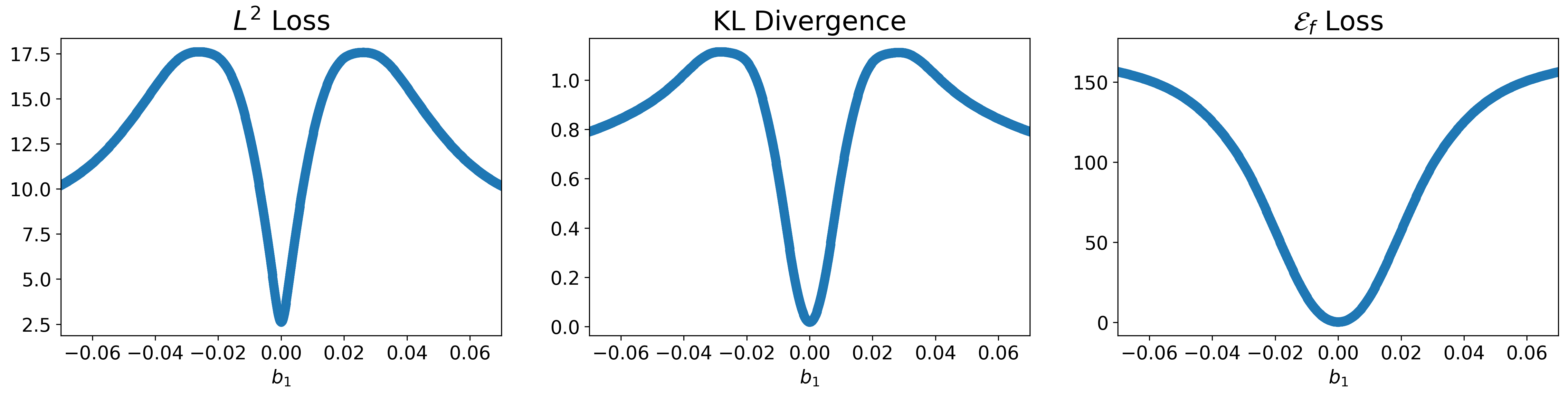
Figure 5: Landscape of the Bump-on-Tail instability on the domain $[-0.07,0.07]$ for $b_{1}$ for (4.1). The objective functions are ($L^{2}$) (left), (KL) (center), and (EE)(right).

For Choice B, we extend the analysis to a two-parameter sweep by varying the pair $(b_{1},b_{2})$ over three pre-defined domains ($[-1,1]^{2}$, $[-0.1,0.1]^{2}$, and $[-0.001,0.003]^{2}$). The near-field region is shifted due to the new location of the global minimum in this case.

Figure 6 displays the values of the three objective functions (($L^{2}$), (KL), and (EE)) across the three domains. The conclusions drawn from the two-stream example continue hold, and in some cases even more pronounced. Notably, in the far-field region, the electric energy objective (EE), maintains a relatively convex structure and does not exhibit global minima for large values of $b_{1}$ and $b_{2}$. This observation indicates that an excessively strong external electric field does not always produce a correspondingly small self-generated electric field.

Figure 6: Landscape of the Bump-on-Tail instability with on the domain $[-1,1]^{2}$ (top), $[-0.1,0.1]^{2}$ (center) and, $[-0.001,0.003]^{2}$ (bottom) for $(b_{1},b_{2})$ for (4.2). The objective functions are ($L^{2}$) (left), (KL) (center), and (EE)(right).

5 Solving the PDE-constrained optimization problem

In this section, we present the numerical results obtained from solving (2.6) using Algorithm 1 to address the forward system described by (2.1). The computation was performed on an NVIDIA GeForce RTX 4090 GPU with 24 GB of memory. For the forward simulation, the phase space was discretized with $M=256$ mesh points, and the time domain was discretized using a time step of $\Delta t=0.1$. Each PDE solve can be completed within 5 seconds. Optimization was carried out using automatic differentiation, facilitated by the Python library JAX [4], to compute the required gradients.

The plots shown in Section 4 suggest that the landscape for the objectives ($L^{2}$) or (KL) are rather similar. Therefore we expect the performance of optimization solvers with these objectives would be similar as well. The rest of this section, we perform numerical studies only on (KL) and (EE).

The landscape plots only provide some suggestions on the performance of optimization solvers. Indeed, for local solvers such as gradient descent, that can only sees local behavior of objective functions, the solutions are trapped in local minimum, and thus placing the initial guess in the global basin is crucial. On the other hand, solvers have their non-convex extensions. One such possibility is to integrate the linesearch technique, which allows iterations to jump out of local minima. This can potentially relax the requirement for a good initial guess.

Another strategy typically deployed in optimization is “over-parameterization.” This is to increase the number of unknowns and adjustable parameters, and thus formulating the problem in a higher-dimensional space. In this setting, it is very likely that the dimension of the global optima manifold increases, and so the chance of obtaining optimal points.

For these reasons, we numerically investigate the solvers’ performance on two physics scenarios, Two Stream instability and Bump-on-Tail instability, respectively, in three distinct dimensions of variations:

• Solvers can be either local or adaptive/global;

  • Local solver. There are many kinds of local solvers. We adopt the simplest gradient descent with constant stepsize. The stepsize is small enough ($1e-8$, $1e-9$) that one can essentially view the optimization iteration as a gradient flow along the landscape.

  • Adaptive/global solver. There are also many choices of adaptive solvers. To be more comparable with the choice of local solver (GD), we select GD with linesearch correction as our adaptive solver. The linesearch will satisfy the strong Wolfe condition that we briefly describe below.

    Denoting the GD with stepsize $\alpha_{n}$ at $n$-th iteration for minimizing a function $F$:

    $$x_{n+1}=x_{n}-\alpha_{n}\nabla F(x_{n})\,.$$

    Linesearch is imposed to ensure that the choice of $\alpha_{n}$ provides sufficient decrease. The “sufficiency” is quantified by the following:

    $$F(x_{n}-\alpha_{n}\nabla F(x_{n})) \leq F(x_{n})-c_{1}\alpha_{n}\|\nabla F(x_{n})\|^{2}$$

    $$|[\nabla F(x_{n}-\alpha_{n}\nabla F(x_{n}))]^{\top}\nabla F(x_{n})| \leq c_{2}\|\nabla F(x_{n})\|^{2}$$

    for $0<c_{1}<c_{2}<1$. Namely, either the value of the new update is sufficiently smaller than the current value, or the new update has a gradient almost parallel to that of the old one. In particular, we use $c_{1}=10^{-4}$ and $c_{2}=0.9$.

• Initial guess can be close, or far away from the optimum points;

  More specifically, the three kinds of initializations are

  • Far initialization: $(\bm{a},\bm{b})\in[-1,1]^{2N}$,

  • Mid-range initialization: $(\bm{a},\bm{b})\in[-0.05,0.05]^{2N}$,

  • Near initialization: $(\bm{a},\bm{b})\in[-0.003,0.001]^{2N}$ for Two Stream and $(\bm{a},\bm{b})\in[-0.001,0.003]^{2N}$ for Bump-on-Tail.

  The scaling are termed “far”, “mid-range” and “near” are closely tied to the landscapes we found on Section 4.

• Optimization conducted with either $2$ (under or properly parameterized) or $14$ (over-parameterized) variables.

  According to the definition of the control term (2.5), $H$ is composed of Fourier modes. The terminology “under/properly” or “over” have blurred scientific meanings. Roughly speaking, a system is “over-parameterized” if one can find a configuration that already performs optimization well with a smaller set of parameters. We perform the study with

  • Under/properly parameterized:

    $$H(x;b_{1},b_{2})=b_{1}\sin(k_{0}x)+b_{2}\sin(2k_{0}x)\,,$$ (5.1)

  • Over-parameterized:

    $$H(x;\bm{a},\bm{b})=\sum_{k=1}^{14}a_{k}\cos\left(kk_{0}x\right)+b_{k}\sin\left(kk_{0}x\right)$$ (5.2)

    where $(\bm{a},\bm{b})=((a_{1},...,a_{14}),(b_{1},...,b_{14}))$.

5.1 Two Stream example

We summarize results for controlling two-stream instability, using the equilibrium state and initial condition presented in (2.9)-(2.10). All numerical results are presented in Table 1 that shows the final distribution function $f_{T}[H]$ with $H$ found by the optimization solver. Also, a more detailed summary of each experiment can be found in Appendix A.1. The stepsize used for the constant stepsize gradient descent is $10^{-8}$.

		Under-parametrized		Over-parametrized
Init.	Step	(KL)	(EE)	(KL)	(EE)
Far	Adaptive
		(see Figure 7)	(see Figure 13)	(see Figure 19)	(see Figure 25)
	Local
		(see Figure 8)	(see Figure 14)	(see Figure 20)	(see Figure 26)
Mid	Adaptive
		(see Figure 9)	(see Figure 15)	(see Figure 21)	(see Figure 27)
	Local
		(see Figure 10)	(see Figure 16)	(see Figure 22)	(see Figure 28)
Near	Adaptive
		(see Figure 11)	(see Figure 17)	(see Figure 23)	(see Figure 29)
	Local
		(see Figure 12)	(see Figure 18)	(see Figure 24)	(see Figure 30)

Table 1: Summary of results for the Two Stream equilibrium.

Multiple conclusions can be drawn.

• Local solver with near-optimal initialization always stabilize the system, and such stability is achieved in both $2$-parameter regime, and $14$-parameter regime, as seen in Figures 12, 18, 24 and 30. This signifies the importance of making a good initial guess. Making a good initial guess is usually not a feasible task for a classical PDE-constrained optimization. Fortunately, for plasma control, the study of the dispersion relation can potentially identify the global basin, see discussion in Section 3.

• Adaptive solver is not compatible with the objective function (EE), as seen in Figures 13, 29, 15, 27 and 29. Indeed, as shown in Figure 4, (EE) has very low evaluation when parameters are very large. When adaptive solvers such as GD with linesearch are deployed, the searching can take the iteration very far into the large parameter domain. This corresponds to the situation when the external field is extremely strong and it completely dominates the whole plasma behavior. When it happens, the self-generated electric field is indeed very small, but the solution renders meaningless physics. The only exception in this case is to set the initial data from a near-optimal initialization. The basin is convex enough to control the linesearch’s performance, see Figure 17.

• The KL divergence does not seem to be a good metric for suppressing instability. Good suppression solution is only observed when initialization is near-optimal already (see Figures 11, 12 and 24). With neither adaptive or local solver, in neither under-parameterized or over-parameterized regime, KL metric does not return a satisfactory solution as long as initialization is not near-optimal.

• Counter-intuitively, over-parametrization in this setting does not seem to bring too much benefit (comparing the third/forth columns with the first/second columns), with the only exception being the use of an adaptive solver for minimizing KL with a far-away initialization (comparing Figure 19 with Figure 7).

5.2 Bump-on-Tail example

For the Bump-on-Tail example (see Table 2 and Appendix A.2), most of the observations drawn from the previous example still hold true, or are even more prominent, except for the comparison between under- and over-parametrized scenarios. In particular, comparing over-parametrized results with those for under-parameterized using (EE) in the near-optimal initialization with local solver, it is evident over-parametrization significantly improves the stability (see Figures 54 and 42). This can potentially be explained by the fact that Bump-on-Tail distribution has more fine features and thus requires more Fourier modes for a successful suppression of instabilities.

		Under-parametrized		Over-parametrized
Init.	Step	(KL)	(EE)	(KL)	(EE)
Far	Adaptive
		(see Figure 31)	(see Figure 37)	(see Figure 43)	(see Figure 49)
	Local
		(see Figure 32)	(see Figure 38)	(see Figure 44)	(see Figure 50)
Mid	Adaptive
		(see Figure 33)	(see Figure 39)	(see Figure 45)	(see Figure 51)
	Local
		(see Figure 34)	(see Figure 40)	(see Figure 46)	(see Figure 52)
Near	Adaptive
		(see Figure 35)	(see Figure 41)	(see Figure 47)	(see Figure 53)
	Local
		(see Figure 36)	(see Figure 42)	(see Figure 48)	(see Figure 54)

Table 2: Summary of results for the Bump-on-Tail equilibrium.

Appendix A Summary of results

In this section we present in detail the results seen in Tables 1 and 2.

A.1 Two Stream example

Figure 7: Simulation of (2.1) with under-parametrized $H$ obtained from (2.6) using (KL) with far initialization using GD with linesearch. From left to right and top to bottom: $f[H](T=30,x,v)$, $|f[H](T,x,v)-f_{\text{eq}}(v)|$, $H$ and $E_{f[H]}(t,x)$, $\mathcal{E}_{f[H]}(t)$, convergence of objective and, trajectory over the landscape of the objective (yellow dot is initial guess).

Figure 8: Simulation of (2.1) with under-parametrized $H$ obtained from (2.6) using (KL) with far initialization using GD with constant stepsize. From left to right and top to bottom: $f[H](T=30,x,v)$, $|f[H](T,x,v)-f_{\text{eq}}(v)|$, $H$ and $E_{f[H]}(t,x)$, $\mathcal{E}_{f[H]}(t)$, convergence of objective and, trajectory over the landscape of the objective (yellow dot is initial guess).

Figure 9: Simulation of (2.1) with under-parametrized $H$ obtained from (2.6) using (KL) with near initialization using GD with linesearch. From left to right and top to bottom: $f[H](T=30,x,v)$, $|f[H](T,x,v)-f_{\text{eq}}(v)|$, $H$ and $E_{f[H]}(t,x)$, $\mathcal{E}_{f[H]}(t)$, convergence of objective and, trajectory over the landscape of the objective (yellow dot is initial guess).

Figure 10: Simulation of (2.1) with under-parametrized $H$ obtained from (2.6) using (KL) with near initialization using GD with constant stepsize. From left to right and top to bottom: $f[H](T=30,x,v)$, $|f[H](T,x,v)-f_{\text{eq}}(v)|$, $H$ and $E_{f[H]}(t,x)$, $\mathcal{E}_{f[H]}(t)$, convergence of objective and, trajectory over the landscape of the objective (yellow dot is initial guess).

Figure 11: Simulation of (2.1) with under-parametrized $H$ obtained from (2.6) using (KL) with local initialization using GD with linesearch. From left to right and top to bottom: $f[H](T=30,x,v)$, $|f[H](T,x,v)-f_{\text{eq}}(v)|$, $H$ and $E_{f[H]}(t,x)$, $\mathcal{E}_{f[H]}(t)$, convergence of objective and, trajectory over the landscape of the objective (yellow dot is initial guess).

Figure 12: Simulation of (2.1) with under-parametrized $H$ obtained from (2.6) using (KL) with local initialization using GD with constant stepsize. From left to right and top to bottom: $f[H](T=30,x,v)$, $|f[H](T,x,v)-f_{\text{eq}}(v)|$, $H$ and $E_{f[H]}(t,x)$, $\mathcal{E}_{f[H]}(t)$, convergence of objective and, trajectory over the landscape of the objective (yellow dot is initial guess).

Figure 13: Simulation of (2.1) with under-parametrized $H$ obtained from (2.6) using (EE) with far initialization using GD with linesearch. From left to right and top to bottom: $f[H](T=30,x,v)$, $|f[H](T,x,v)-f_{\text{eq}}(v)|$, $H$ and $E_{f[H]}(t,x)$, $\mathcal{E}_{f[H]}(t)$, convergence of objective and, trajectory over the landscape of the objective (yellow dot is initial guess).

Figure 14: Simulation of (2.1) with under-parametrized $H$ obtained from (2.6) using (EE) with far initialization using GD with constant stepsize. From left to right and top to bottom: $f[H](T=30,x,v)$, $|f[H](T,x,v)-f_{\text{eq}}(v)|$, $H$ and $E_{f[H]}(T,x)$, $E_{f[H]}(t,x)$, $\mathcal{E}_{f[H]}(t)$ and, convergence of objective.

Figure 15: Simulation of (2.1) with under-parametrized $H$ obtained from (2.6) using (EE) with near initialization using GD with linesearch. From left to right and top to bottom: $f[H](T=30,x,v)$, $|f[H](T,x,v)-f_{\text{eq}}(v)|$, $H$ and $E_{f[H]}(t,x)$, $\mathcal{E}_{f[H]}(t)$, convergence of objective and, trajectory over the landscape of the objective (yellow dot is initial guess).

Figure 16: Simulation of (2.1) using (EE) with under-parametrized $H$ obtained from (2.6) with near initialization using GD with constant stepsize. From left to right and top to bottom: $f[H](T=30,x,v)$, $|f[H](T,x,v)-f_{\text{eq}}(v)|$, $H$ and $E_{f[H]}(t,x)$, $\mathcal{E}_{f[H]}(t)$, convergence of objective and, trajectory over the landscape of the objective (yellow dot is initial guess).

Figure 17: Simulation of (2.1) with under-parametrized $H$ obtained from (2.6) using (EE) with local initialization using GD with linesearch. From left to right and top to bottom: $f[H](T=30,x,v)$, $|f[H](T,x,v)-f_{\text{eq}}(v)|$, $H$ and $E_{f[H]}(t,x)$, $\mathcal{E}_{f[H]}(t)$, convergence of objective and, trajectory over the landscape of the objective (yellow dot is initial guess).

Figure 18: Simulation of (2.1) using (EE) with under-parametrized $H$ obtained from (2.6) with local initialization using GD with constant stepsize. From left to right and top to bottom: $f[H](T=30,x,v)$, $|f[H](T,x,v)-f_{\text{eq}}(v)|$, $H$ and $E_{f[H]}(t,x)$, $\mathcal{E}_{f[H]}(t)$, convergence of objective and, trajectory over the landscape of the objective (yellow dot is initial guess).

Figure 19: Simulation of (2.1) with over-parametrized $H$ obtained from (2.6) using (KL) with far initialization using GD with linesearch. From left to right and top to bottom: $f[H](T=30,x,v)$, $|f[H](T,x,v)-f_{\text{eq}}(v)|$, $H$ and $E_{f[H]}(t,x)$, $\mathcal{E}_{f[H]}(t)$, convergence of objective and, trajectory over the landscape of the objective (yellow dot is initial guess).

Figure 20: Simulation of (2.1) with over-parametrized $H$ obtained from (2.6) using (KL) with far initialization using GD with constant stepsize. From left to right and top to bottom: $f[H](T=30,x,v)$, $|f[H](T,x,v)-f_{\text{eq}}(v)|$, $H$ and $E_{f[H]}(t,x)$, $\mathcal{E}_{f[H]}(t)$, convergence of objective and, trajectory over the landscape of the objective (yellow dot is initial guess).

Figure 21: Simulation of (2.1) with over-parametrized $H$ obtained from (2.6) using (KL) with near initialization using GD with linesearch. From left to right and top to bottom: $f[H](T=30,x,v)$, $|f[H](T,x,v)-f_{\text{eq}}(v)|$, $H$ and $E_{f[H]}(t,x)$, $\mathcal{E}_{f[H]}(t)$, convergence of objective and, trajectory over the landscape of the objective (yellow dot is initial guess).

Figure 22: Simulation of (2.1) with over-parametrized $H$ obtained from (2.6) using (KL) with near initialization using GD with constant stepsize. From left to right and top to bottom: $f[H](T=30,x,v)$, $|f[H](T,x,v)-f_{\text{eq}}(v)|$, $H$ and $E_{f[H]}(t,x)$, $\mathcal{E}_{f[H]}(t)$, convergence of objective and, trajectory over the landscape of the objective (yellow dot is initial guess).

Figure 23: Simulation of (2.1) with over-parametrized $H$ obtained from (2.6) using (KL) with local initialization using GD with linesearch. From left to right and top to bottom: $f[H](T=30,x,v)$, $|f[H](T,x,v)-f_{\text{eq}}(v)|$, $H$ and $E_{f[H]}(t,x)$, $\mathcal{E}_{f[H]}(t)$, convergence of objective and, trajectory over the landscape of the objective (yellow dot is initial guess).

Figure 24: Simulation of (2.1) with over-parametrized $H$ obtained from (2.6) using (KL) with local initialization using GD with constant stepsize. From left to right and top to bottom: $f[H](T=30,x,v)$, $|f[H](T,x,v)-f_{\text{eq}}(v)|$, $H$ and $E_{f[H]}(t,x)$, $\mathcal{E}_{f[H]}(t)$, convergence of objective and, trajectory over the landscape of the objective (yellow dot is initial guess).

Figure 25: Simulation of (2.1) with under-parametrized $H$ obtained from (2.6) using (EE) with far initialization using GD with linesearch. From left to right and top to bottom: $f[H](T=30,x,v)$, $|f[H](T,x,v)-f_{\text{eq}}(v)|$, $H$ and $E_{f[H]}(t,x)$, $\mathcal{E}_{f[H]}(t)$, convergence of objective and, trajectory over the landscape of the objective (yellow dot is initial guess).

Figure 26: Simulation of (2.1) with over-parametrized $H$ obtained from (2.6) using (EE) with far initialization using GD with constant stepsize. From left to right and top to bottom: $f[H](T=30,x,v)$, $|f[H](T,x,v)-f_{\text{eq}}(v)|$, $H$ and $E_{f[H]}(t,x)$, $\mathcal{E}_{f[H]}(t)$, convergence of objective and, trajectory over the landscape of the objective (yellow dot is initial guess).

Figure 27: Simulation of (2.1) with over-parametrized $H$ obtained from (2.6) using (EE) with near initialization using GD with linesearch. From left to right and top to bottom: $f[H](T=30,x,v)$, $|f[H](T,x,v)-f_{\text{eq}}(v)|$, $H$ and $E_{f[H]}(t,x)$, $\mathcal{E}_{f[H]}(t)$, convergence of objective and, trajectory over the landscape of the objective (yellow dot is initial guess).

Figure 28: Simulation of (2.1) using (EE) with over-parametrized $H$ obtained from (2.6) with near initialization using GD with constant stepsize. From left to right and top to bottom: $f[H](T=30,x,v)$, $|f[H](T,x,v)-f_{\text{eq}}(v)|$, $H$ and $E_{f[H]}(t,x)$, $\mathcal{E}_{f[H]}(t)$, convergence of objective and, trajectory over the landscape of the objective (yellow dot is initial guess).

Figure 29: Simulation of (2.1) with over-parametrized $H$ obtained from (2.6) using (EE) with local initialization using GD with linesearch. From left to right and top to bottom: $f[H](T=30,x,v)$, $|f[H](T,x,v)-f_{\text{eq}}(v)|$, $H$ and $E_{f[H]}(t,x)$, $\mathcal{E}_{f[H]}(t)$, convergence of objective and, trajectory over the landscape of the objective (yellow dot is initial guess).

Figure 30: Simulation of (2.1) using (EE) with over-parametrized $H$ obtained from (2.6) with local initialization using GD with constant stepsize. From left to right and top to bottom: $f[H](T=30,x,v)$, $|f[H](T,x,v)-f_{\text{eq}}(v)|$, $H$ and $E_{f[H]}(t,x)$, $\mathcal{E}_{f[H]}(t)$, convergence of objective and, trajectory over the landscape of the objective (yellow dot is initial guess).

A.2 Bump-on-Tail example

Figure 31: Simulation of (2.1) with under-parametrized $H$ obtained from (2.6) using (KL) with far initialization using GD with linesearch. From left to right and top to bottom: $f[H](T=30,x,v)$, $|f[H](T,x,v)-f_{\text{eq}}(v)|$, $H$ and $E_{f[H]}(t,x)$, $\mathcal{E}_{f[H]}(t)$, convergence of objective and, trajectory over the landscape of the objective (yellow dot is initial guess).

Figure 32: Simulation of (2.1) with under-parametrized $H$ obtained from (2.6) using (KL) with far initialization using GD with constant stepsize. From left to right and top to bottom: $f[H](T=30,x,v)$, $|f[H](T,x,v)-f_{\text{eq}}(v)|$, $H$ and $E_{f[H]}(t,x)$, $\mathcal{E}_{f[H]}(t)$, convergence of objective and, trajectory over the landscape of the objective (yellow dot is initial guess).

Figure 33: Simulation of (2.1) with under-parametrized $H$ obtained from (2.6) using (KL) with near initialization using GD with linesearch. From left to right and top to bottom: $f[H](T=30,x,v)$, $|f[H](T,x,v)-f_{\text{eq}}(v)|$, $H$ and $E_{f[H]}(t,x)$, $\mathcal{E}_{f[H]}(t)$, convergence of objective and, trajectory over the landscape of the objective (yellow dot is initial guess).

Figure 34: Simulation of (2.1) with under-parametrized $H$ obtained from (2.6) using (KL) with near initialization using GD with constant stepsize. From left to right and top to bottom: $f[H](T=30,x,v)$, $|f[H](T,x,v)-f_{\text{eq}}(v)|$, $H$ and $E_{f[H]}(t,x)$, $\mathcal{E}_{f[H]}(t)$, convergence of objective and, trajectory over the landscape of the objective (yellow dot is initial guess).

Figure 35: Simulation of (2.1) with under-parametrized $H$ obtained from (2.6) using (KL) with local initialization using GD with linesearch. From left to right and top to bottom: $f[H](T=30,x,v)$, $|f[H](T,x,v)-f_{\text{eq}}(v)|$, $H$ and $E_{f[H]}(t,x)$, $\mathcal{E}_{f[H]}(t)$, convergence of objective and, trajectory over the landscape of the objective (yellow dot is initial guess).

Figure 36: Simulation of (2.1) with under-parametrized $H$ obtained from (2.6) using (KL) with local initialization using GD with constant stepsize. From left to right and top to bottom: $f[H](T=30,x,v)$, $|f[H](T,x,v)-f_{\text{eq}}(v)|$, $H$ and $E_{f[H]}(t,x)$, $\mathcal{E}_{f[H]}(t)$, convergence of objective and, trajectory over the landscape of the objective (yellow dot is initial guess).

Figure 37: Simulation of (2.1) with under-parametrized $H$ obtained from (2.6) using (EE) with far initialization using GD with linesearch. From left to right and top to bottom: $f[H](T=30,x,v)$, $|f[H](T,x,v)-f_{\text{eq}}(v)|$, $H$ and $E_{f[H]}(t,x)$, $\mathcal{E}_{f[H]}(t)$, convergence of objective and, trajectory over the landscape of the objective (yellow dot is initial guess).

Figure 38: Simulation of (2.1) with under-parametrized $H$ obtained from (2.6) using (EE) with far initialization using GD with constant stepsize. From left to right and top to bottom: $f[H](T=30,x,v)$, $|f[H](T,x,v)-f_{\text{eq}}(v)|$, $H$ and $E_{f[H]}(t,x)$, $\mathcal{E}_{f[H]}(t)$, convergence of objective and, trajectory over the landscape of the objective (yellow dot is initial guess).

Figure 39: Simulation of (2.1) with under-parametrized $H$ obtained from (2.6) using (EE) with near initialization using GD with linesearch. From left to right and top to bottom: $f[H](T=30,x,v)$, $|f[H](T,x,v)-f_{\text{eq}}(v)|$, $H$ and $E_{f[H]}(t,x)$, $\mathcal{E}_{f[H]}(t)$, convergence of objective and, trajectory over the landscape of the objective (yellow dot is initial guess).

Figure 40: Simulation of (2.1) using (EE) with under-parametrized $H$ obtained from (2.6) with near initialization using GD with constant stepsize. From left to right and top to bottom: $f[H](T=30,x,v)$, $|f[H](T,x,v)-f_{\text{eq}}(v)|$, $H$ and $E_{f[H]}(t,x)$, $\mathcal{E}_{f[H]}(t)$, convergence of objective and, trajectory over the landscape of the objective (yellow dot is initial guess).

Figure 41: Simulation of (2.1) with under-parametrized $H$ obtained from (2.6) using (EE) with local initialization using GD with linesearch. From left to right and top to bottom: $f[H](T=30,x,v)$, $|f[H](T,x,v)-f_{\text{eq}}(v)|$,$H$ and $E_{f[H]}(t,x)$, $\mathcal{E}_{f[H]}(t)$, convergence of objective and, trajectory over the landscape of the objective (yellow dot is initial guess).

Figure 42: Simulation of (2.1) using (EE) with under-parametrized $H$ obtained from (2.6) with local initialization using GD with constant stepsize. From left to right and top to bottom: $f[H](T=30,x,v)$, $|f[H](T,x,v)-f_{\text{eq}}(v)|$, $H$ and $E_{f[H]}(t,x)$, $\mathcal{E}_{f[H]}(t)$, convergence of objective and, trajectory over the landscape of the objective (yellow dot is initial guess).

Figure 43: Simulation of (2.1) with over-parametrized $H$ obtained from (2.6) using (KL) with far initialization using GD with linesearch. From left to right and top to bottom: $f[H](T=30,x,v)$, $|f[H](T,x,v)-f_{\text{eq}}(v)|$, $H$ and $E_{f[H]}(t,x)$, $\mathcal{E}_{f[H]}(t)$, convergence of objective and, trajectory over the landscape of the objective (yellow dot is initial guess).

Figure 44: Simulation of (2.1) with over-parametrized $H$ obtained from (2.6) using (KL) with far initialization using GD with constant stepsize. From left to right and top to bottom: $f[H](T=30,x,v)$, $|f[H](T,x,v)-f_{\text{eq}}(v)|$, $H$ and $E_{f[H]}(t,x)$, $\mathcal{E}_{f[H]}(t)$, convergence of objective and, trajectory over the landscape of the objective (yellow dot is initial guess).

Figure 45: Simulation of (2.1) with over-parametrized $H$ obtained from (2.6) using (KL) with near initialization using GD with linesearch. From left to right and top to bottom: $f[H](T=30,x,v)$, $|f[H](T,x,v)-f_{\text{eq}}(v)|$, $H$ and $E_{f[H]}(t,x)$, $\mathcal{E}_{f[H]}(t)$, convergence of objective and, trajectory over the landscape of the objective (yellow dot is initial guess).

Figure 46: Simulation of (2.1) with over-parametrized $H$ obtained from (2.6) using (KL) with near initialization using GD with constant stepsize. From left to right and top to bottom: $f[H](T=30,x,v)$, $|f[H](T,x,v)-f_{\text{eq}}(v)|$, $H$ and $E_{f[H]}(t,x)$, $\mathcal{E}_{f[H]}(t)$, convergence of objective and, trajectory over the landscape of the objective (yellow dot is initial guess).

Figure 47: Simulation of (2.1) with over-parametrized $H$ obtained from (2.6) using (KL) with local initialization using GD with linesearch. From left to right and top to bottom: $f[H](T=30,x,v)$, $|f[H](T,x,v)-f_{\text{eq}}(v)|$, $H$ and $E_{f[H]}(t,x)$, $\mathcal{E}_{f[H]}(t)$, convergence of objective and, trajectory over the landscape of the objective (yellow dot is initial guess).

Figure 48: Simulation of (2.1) with over-parametrized $H$ obtained from (2.6) using (KL) with local initialization using GD with constant stepsize. From left to right and top to bottom: $f[H](T=30,x,v)$, $|f[H](T,x,v)-f_{\text{eq}}(v)|$, $H$ and $E_{f[H]}(t,x)$, $\mathcal{E}_{f[H]}(t)$, convergence of objective and, trajectory over the landscape of the objective (yellow dot is initial guess).

Figure 49: Simulation of (2.1) with under-parametrized $H$ obtained from (2.6) using (EE) with far initialization using GD with linesearch. From left to right and top to bottom: $f[H](T=30,x,v)$, $|f[H](T,x,v)-f_{\text{eq}}(v)|$, $H$ and $E_{f[H]}(T,x)$, $E_{f[H]}(t,x)$, $\mathcal{E}_{f[H]}(t)$ and, convergence of objective.

Figure 50: Simulation of (2.1) with over-parametrized $H$ obtained from (2.6) using (EE) with far initialization using GD with constant stepsize. From left to right and top to bottom: $f[H](T=30,x,v)$, $|f[H](T,x,v)-f_{\text{eq}}(v)|$, $H$ and $E_{f[H]}(t,x)$, $\mathcal{E}_{f[H]}(t)$, convergence of objective and, trajectory over the landscape of the objective (yellow dot is initial guess).

Figure 51: Simulation of (2.1) with over-parametrized $H$ obtained from (2.6) using (EE) with near initialization using GD with linesearch. From left to right and top to bottom: $f[H](T=30,x,v)$, $|f[H](T,x,v)-f_{\text{eq}}(v)|$, $H$ and $E_{f[H]}(t,x)$, $\mathcal{E}_{f[H]}(t)$, convergence of objective and, trajectory over the landscape of the objective (yellow dot is initial guess).

Figure 52: Simulation of (2.1) using (EE) with over-parametrized $H$ obtained from (2.6) with near initialization using GD with constant stepsize. From left to right and top to bottom: $f[H](T=30,x,v)$, $|f[H](T,x,v)-f_{\text{eq}}(v)|$, $H$ and $E_{f[H]}(t,x)$, $\mathcal{E}_{f[H]}(t)$, convergence of objective and, trajectory over the landscape of the objective (yellow dot is initial guess).

Figure 53: Simulation of (2.1) with over-parametrized $H$ obtained from (2.6) using (EE) with local initialization using GD with linesearch. From left to right and top to bottom: $f[H](T=30,x,v)$, $|f[H](T,x,v)-f_{\text{eq}}(v)|$, $H$ and $E_{f[H]}(t,x)$, $\mathcal{E}_{f[H]}(t)$, convergence of objective and, trajectory over the landscape of the objective (yellow dot is initial guess).

Figure 54: Simulation of (2.1) using (EE) with over-parametrized $H$ obtained from (2.6) with local initialization using GD with constant stepsize. From left to right and top to bottom: $f[H](T=30,x,v)$, $|f[H](T,x,v)-f_{\text{eq}}(v)|$, $H$ and $E_{f[H]}(t,x)$, $\mathcal{E}_{f[H]}(t)$, convergence of objective and, trajectory over the landscape of the objective (yellow dot is initial guess).

References

- [1] Giacomo Albi, Giacomo Dimarco, Federica Ferrarese and Lorenzo Pareschi “Instantaneous control strategies for magnetically confined fusion plasma” In Journal of Computational Physics 527, 2025, pp. 113804 DOI: https://doi.org/10.1016/j.jcp.2025.113804
- [2] Jan Bartsch, Patrik Knopf, Stefania Scheurer and Jörg Weber “Controlling a Vlasov–Poisson Plasma by a Particle-in-Cell Method Based on a Monte Carlo Framework” In SIAM Journal on Control and Optimization 62.4, 2024, pp. 1977–2011 DOI: 10.1137/23M1563852
- [3] James Bialek, Allen H. Boozer, M.. Mauel and G.. Navratil “Modeling of active control of external magnetohydrodynamic instabilities” In Physics of Plasmas 8.5, 2001, pp. 2170–2180 DOI: 10.1063/1.1362532
- [4] James Bradbury et al. “JAX: composable transformations of Python+NumPy programs”, 2018 URL: http://github.com/jax-ml/jax
- [5] KTAL Burm “Plasma: The fourth state of matter” In Plasma Chemistry and Plasma Processing 32 Springer, 2012, pp. 401–407
- [6] Shi Chen, Zhiyan Ding, Qin Li and Leonardo Zepeda-Núñez “High-Frequency Limit of the Inverse Scattering Problem: Asymptotic Convergence from Inverse Helmholtz to Inverse Liouville” In SIAM Journal on Imaging Sciences 16.1, 2023, pp. 111–143 DOI: 10.1137/22M147075X
- [7] Chio-Zong Cheng and Georg Knorr “The integration of the Vlasov equation in configuration space” In Journal of Computational Physics 22.3 Elsevier, 1976, pp. 330–351
- [8] N. Crouseilles, M. Mehrenberger and Vecil, F. “Discontinuous Galerkin semi-Lagrangian method for Vlasov-Poisson” In ESAIM: Proc. 32, 2011, pp. 211–230 DOI: 10.1051/proc/2011022
- [9] Lukas Einkemmer “A performance comparison of semi-Lagrangian discontinuous Galerkin and spline based Vlasov solvers in four dimensions” In Journal of Computational Physics 376 Elsevier, 2019, pp. 937–951
- [10] Lukas Einkemmer, Qin Li, Clément Mouhot and Yukun Yue “Control of instability in a Vlasov-Poisson system through an external electric field” In Journal of Computational Physics 530, 2025, pp. 113904 DOI: https://doi.org/10.1016/j.jcp.2025.113904
- [11] Lukas Einkemmer, Qin Li, Li Wang and Yang Yunan “Suppressing instability in a Vlasov–Poisson system by an external electric field through constrained optimization” In Journal of Computational Physics 498, 2024, pp. 112662 DOI: https://doi.org/10.1016/j.jcp.2023.112662
- [12] Björn Engquist and Yunan Yang “Optimal Transport Based Seismic Inversion:Beyond Cycle Skipping” In Communications on Pure and Applied Mathematics 75.10, 2022, pp. 2201–2244 DOI: https://doi.org/10.1002/cpa.21990
- [13] Francis Filbet and Eric Sonnendrücker “Comparison of Eulerian Vlasov solvers” In Computer Physics Communications 150.3 Elsevier, 2003, pp. 247–266
- [14] Richard Fitzpatrick “Plasma physics: an introduction” Crc Press, 2022
- [15] D Frank-Kamenetskii “Plasma: the fourth state of matter” Springer Science & Business Media, 2012
- [16] Olivier Glass “On the controllability of the Vlasov–Poisson system” In Journal of Differential Equations 195.2, 2003, pp. 332–379 DOI: https://doi.org/10.1016/S0022-0396(03)00066-4
- [17] Olivier Glass and Daniel Han-Kwan “On the controllability of the Vlasov–Poisson system in the presence of external force fields” In Journal of Differential Equations 252.10, 2012, pp. 5453–5491 DOI: https://doi.org/10.1016/j.jde.2012.02.007
- [18] Setsuo Ichimaru “Nuclear fusion in dense plasmas” In reviews of modern physics 65.2 APS, 1993, pp. 255
- [19] S. Kawata, T. Karino and Y.J. Gu “Dynamic stabilization of plasma instability” In High Power Laser Science and Engineering 7 Cambridge University Press, 2019, pp. e3
- [20] A.J. Klimas and W.M. Farrell “A Splitting Algorithm for Vlasov Simulation with Filamentation Filtration” In Journal of Computational Physics 110.1, 1994, pp. 150–163 DOI: https://doi.org/10.1006/jcph.1994.1011
- [21] Alexander J. Klimas and Adolfo.. Viñas “Absence of recurrence in Fourier–Fourier transformed Vlasov–Poisson simulations” In Journal of Plasma Physics 84.4, 2018, pp. 905840405 DOI: 10.1017/S0022377818000776
- [22] Patrik Knopf “Confined steady states of a Vlasov-Poisson plasma in an infinitely long cylinder” In Mathematical Methods in the Applied Sciences 42.18, 2019, pp. 6369–6384 DOI: https://doi.org/10.1002/mma.5728
- [23] Patrik Knopf “Optimal control of a Vlasov–Poisson plasma by an external magnetic field” In Calculus of Variations and Partial Differential Equations 57.5, 2018 DOI: 10.1007/s00526-018-1407-x
- [24] Kenro Miyamoto “Plasma physics for nuclear fusion” Massachusetts Institute of Technology, Cambridge, MA, 1980
- [25] Oliver Penrose “Electrostatic instabilities of a uniform non-Maxwellian plasma” In The Physics of Fluids 3.2 American Institute of Physics, 1960, pp. 258–265
- [26] Jing-Mei Qiu and Chi-Wang Shu “Positivity preserving semi-Lagrangian discontinuous Galerkin formulation: theoretical analysis and application to the Vlasov–Poisson system” In Journal of Computational Physics 230.23 Elsevier, 2011, pp. 8386–8409
- [27] James A. Rossmanith and David C. Seal “A positivity-preserving high-order semi-Lagrangian discontinuous Galerkin scheme for the Vlasov–Poisson equations” In Journal of Computational Physics 230.16, 2011, pp. 6203–6232 DOI: https://doi.org/10.1016/j.jcp.2011.04.018
- [28] Eric Sonnendrücker, Jean Roche, Pierre Bertrand and Alain Ghizzo “The semi-Lagrangian method for the numerical resolution of the Vlasov equation” In Journal of computational physics 149.2 Elsevier, 1999, pp. 201–220
- [29] E.. Strait “Magnetic control of magnetohydrodynamic instabilities in tokamaks” In Physics of Plasmas 22.2, 2014, pp. 021803 DOI: 10.1063/1.4902126
- [30] W.. Symes and J.. Carazzone “Velocity inversion by differential semblance optimization” In GEOPHYSICS 56.5, 1991, pp. 654–663 DOI: 10.1190/1.1443082
- [31] MA Van Zeeland et al. “Beam modulation and bump-on-tail effects on Alfvén eigenmode stability in DIII-D” In Nuclear Fusion 61.6 IOP Publishing, 2021, pp. 066028
- [32] J P Verboncoeur “Particle simulation of plasmas: review and advances” In Plasma Physics and Controlled Fusion 47.5A, 2005, pp. A231 DOI: 10.1088/0741-3335/47/5A/017
- [33] Hartmut Zohm “Magnetohydrodynamic stability of tokamaks” John Wiley & Sons, 2015