MonoDiff9D: Monocular Category-Level 9D Object
Pose Estimation via Diffusion Model
Abstract
Object pose estimation is a core means for robots to understand and interact with their environment. For this task, monocular category-level methods are attractive as they require only a single RGB camera. However, current methods rely on shape priors or CAD models of the intra-class known objects. We propose a diffusion-based monocular category-level 9D object pose generation method, MonoDiff9D. Our motivation is to leverage the probabilistic nature of diffusion models to alleviate the need for shape priors, CAD models, or depth sensors for intra-class unknown object pose estimation. We first estimate coarse depth via DINOv2 from the monocular image in a zero-shot manner and convert it into a point cloud. We then fuse the global features of the point cloud with the input image and use the fused features along with the encoded time step to condition MonoDiff9D. Finally, we design a transformer-based denoiser to recover the object pose from Gaussian noise. Extensive experiments on two popular benchmark datasets show that MonoDiff9D achieves state-of-the-art monocular category-level 9D object pose estimation accuracy without the need for shape priors or CAD models at any stage. Our code will be made public at https://github.com/CNJianLiu/MonoDiff9D.
I INTRODUCTION
Nine-degrees-of-freedom (9D) object pose estimation aims to predict the 3D translation, 3D rotation, and 3D size of an object relative to the camera [1, 2, 3, 4, 5, 6]. It plays a crucial role in robotic 3D scene understanding [7, 8, 9, 10, 11, 12]. Early object pose estimation methods are mainly instance-level methods [13, 14, 15, 16, 17, 18]. They achieve good results on specific object instances, but have poor generalization ability. Recently, category-level methods have received extensive research attention due to their ability to generalize to intra-class unknown objects without requiring CAD models of the objects [19, 20, 21, 22, 23, 24, 25].
As one of the pioneers in category-level research, Wang et al. [26] proposed a Normalized Object Coordinate Space (NOCS) for the standardized representation of a category of objects, and used the Umeyama algorithm [27] to match the predicted NOCS shape and the observed object point cloud to solve the pose. Following this, several RGBD-based methods were proposed that fuse the 2D texture and 3D geometric features of the observed object for pose estimation [28, 29, 30, 31, 32, 33]. In addition, some RGBD-based domain adaptation and domain generalization methods have been introduced [34, 35, 36, 37, 38], which aim to reduce the reliance on real-world annotated data. Besides these RGBD-based methods, some depth-based methods have been proposed [39, 40, 41, 42], which further focus on the geometric features of the observed object and then directly regress the object pose. Although these RGBD and depth-based methods achieve superior performance, they exhibit excessive dependence on depth information. Since depth sensors are energy-consuming for robots and most mobile devices (such as mobile phones, tablets, laptops, etc.) are not equipped with them, achieving monocular category-level pose estimation holds significant importance across diverse applications.
To avoid the need for depth sensor, some monocular RGB-based methods have been proposed [44, 45, 46, 47, 48]. Synthesis [44] and MSOS [45] estimate object pose from a single RGB image, however, their performance is greatly limited since a monocular RGB image cannot accurately represent the 3D location and geometric information. More recently, OLD-Net [46] and DMSR [47] first leverage a single RGB image to estimate the depth or sketch of the observed object, and then combine the estimated geometric information and shape priors to reconstruct the NOCS shape of the intra-class unknown object. Next, the 9D object pose is solved through the Umeyama [27] or RANSAC+Perspective-n-Point (PnP) [47] algorithm. Although these methods improve accuracy, they either require the Umeyama algorithm to solve the pose, or the RANSAC algorithm and the PnP procedure to remove outliers and solve the pose, respectively, making them non-differentiable. Furthermore, they all rely on using shape priors or the CAD models of intra-class known objects during training, which need extensive manual effort to obtain.
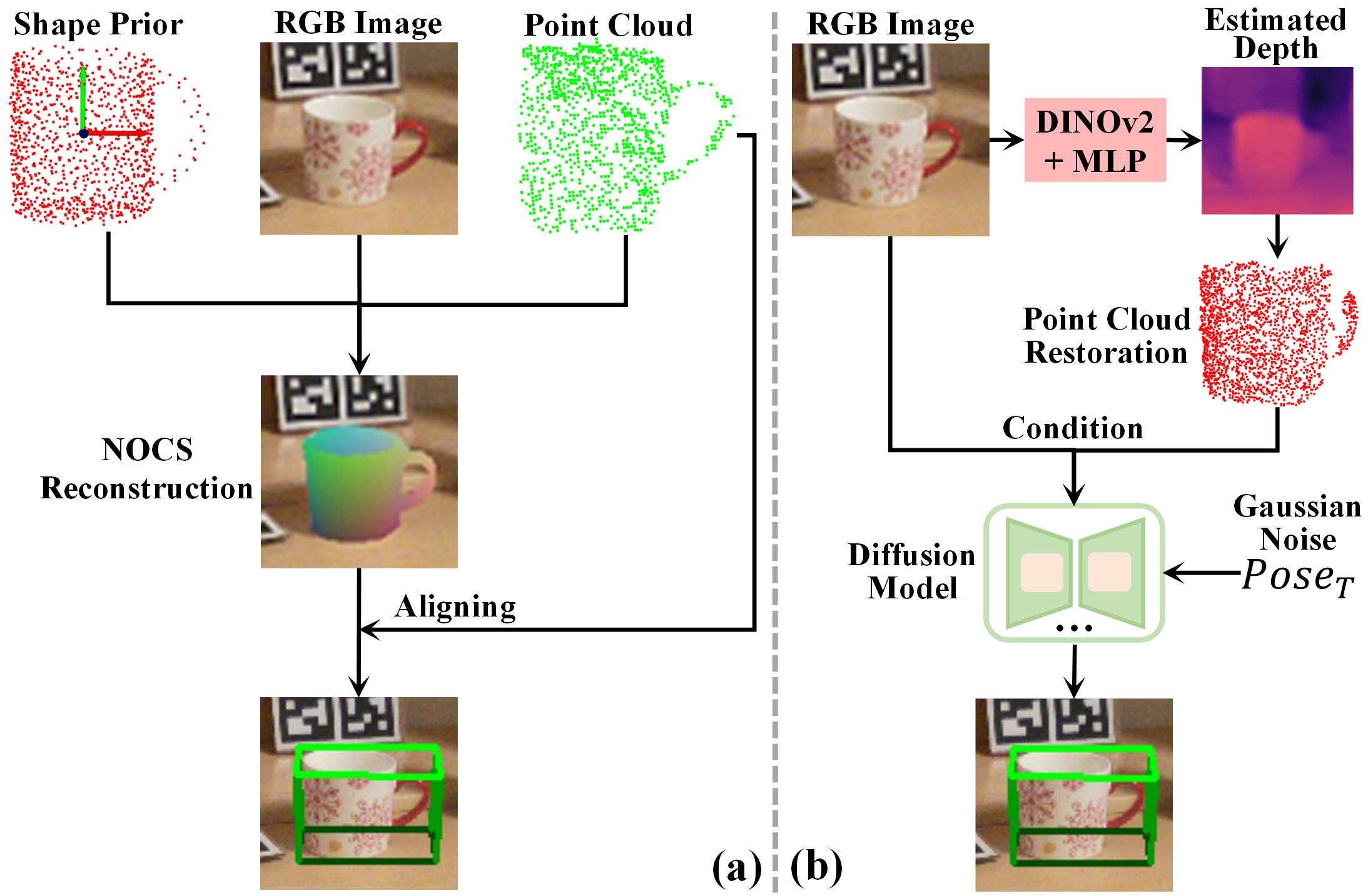
To address the aforementioned challenges, inspired by the prior work Diff9D [49], we propose a differentiable and shape prior-free monocular category-level 9D object pose estimation method, coined MonoDiff9D. Our aim is to exploit the probabilistic nature of the diffusion model to perform intra-class unknown object pose estimation, even in the absence of shape priors, CAD models, or depth sensors. Since the depth image/point cloud can represent the location and geometric information of the object, it is the most critical input for object pose estimation. In particular, estimating 3D object translation from a single RGB image is tricky. Based on this, we propose to leverage the Large Vision Model (LVM) DINOv2 [43] to perform coarse depth estimation from the input RGB image in a zero-shot manner and convert it into a point cloud, thereby introducing the location and geometric information of the observed object to condition the learning of the diffusion model. Since there is still a gap between the DINOv2 estimated and the actual object point clouds, and the complete point cloud may not be restored, we then leverage the self-attention and cross-attention mechanisms to fuse the global features of the RGB image and the estimated point cloud, so that it can pay more attention to the pose-sensitive features of the coarse point cloud. Finally, we design a transformer-based denoiser following the Denoising Diffusion Implicit Model (DDIM) [50] scheduler to recover the object pose from Gaussian noise. A comparison between the shape prior-based RGBD methods and the proposed MonoDiff9D is shown in Fig. 1. Overall, we make the following contributions:
-
•
We propose a diffusion model-based monocular category-level 9D object pose generation framework, designed to enhance generalization to intra-class unknown objects when shape priors and CAD models of intra-class known objects are unavailable.
-
•
We propose LVM-based conditional encoding to introduce coarse location and geometric prompts to condition the learning of the single RGB-based pose diffusion process, and demonstrate that LVM can effectively adapt to this framework without any fine-tuning.
-
•
We demonstrate on two widely used benchmarks that object pose can be recovered from Gaussian noise with state-of-the-art (SOTA) accuracy in near real-time.
II RELATED WORK
We review related category-level object pose estimation works by categorizing them into RGBD-based, depth-based, and RGB-based methods.
II-A RGBD-Based and Depth-Based Methods
SPD [28] first uses the category-level CAD model library to extract shape priors offline. Then, it utilizes shape prior deformation to reconstruct the NOCS shape of intra-class unknown object and leverages the Umeyama algorithm [27] to solve pose. Due to the superior performance achieved by SPD, many other prior-based methods [29, 51, 30, 52, 53] are subsequently proposed. Although these prior-based methods can deal with diverse shape variations between intra-class objects, acquiring shape priors requires manual effort to build the category-level CAD model library. Hence, some prior-free methods like DualPoseNet [31], IST-Net [32], and VI-Net [33] are introduced.
Besides the above RGBD-based methods, there are also some depth-based methods[39, 40, 41, 54, 42]. FS-Net [39] introduces a 3D graph convolution-based framework and performs decoupled regression for 6D pose and 3D size. GPV-Pose [40] and HS-Pose [41] improve the model accuracy by enhancing the learning of pose-sensitive features and designing a hybrid scope feature extraction network, respectively. GenPose [55] introduces a score-based diffusion method for generative 6D object pose estimation. Although these depth-based methods achieve superior performance, they heavily rely on the depth information of the observed object. Due to the energy-consuming nature of depth sensors and most mobile devices are not equipped with them, achieving category-level object pose estimation through a single RGB image is significant for widespread applications.
II-B RGB-Based Methods
Synthesis [44] incorporates a neural synthesis module into a model fitting framework based on optimization to predict object shape and pose concurrently. MSOS [45] predicts the metric scale shape and the NOCS shape of the observed object, and performs a similarity transformation between them to recover the pose. However, their accuracy is greatly limited by the lack of guidance from geometric information. Lin et al. [56] introduced a keypoint-based, single-stage pipeline that operates on a single RGB image. More recently, OLD-Net [46] reconstructs object-level depth and NOCS shape directly from monocular RGB image by deforming category-level shape prior and then aligning them to estimate the object pose. DMSR [47] first predicts the 2.5D sketch and decouples scale recovery based on the shape prior, then reconstructs the NOCS shape for pose estimation. These methods enhance accuracy but typically employ non-differentiable techniques such as the Umeyama algorithm [27] for pose recovery or a combination of RANSAC for outlier removal and the PnP approach for solving pose [47]. Moreover, they often rely on shape priors and CAD models of intra-class known objects during the training process.
Different from the above methods, our MonoDiff9D aims to leverage the LVM DINOv2 [43] to provide geometric guidance to condition the Denoising Diffusion Probabilistic Model (DDPM) [57], achieving differentiable and shape prior-free monocular category-level 9D object pose estimation without using any CAD models during training.
III WORKFLOW of MONODIFF9D
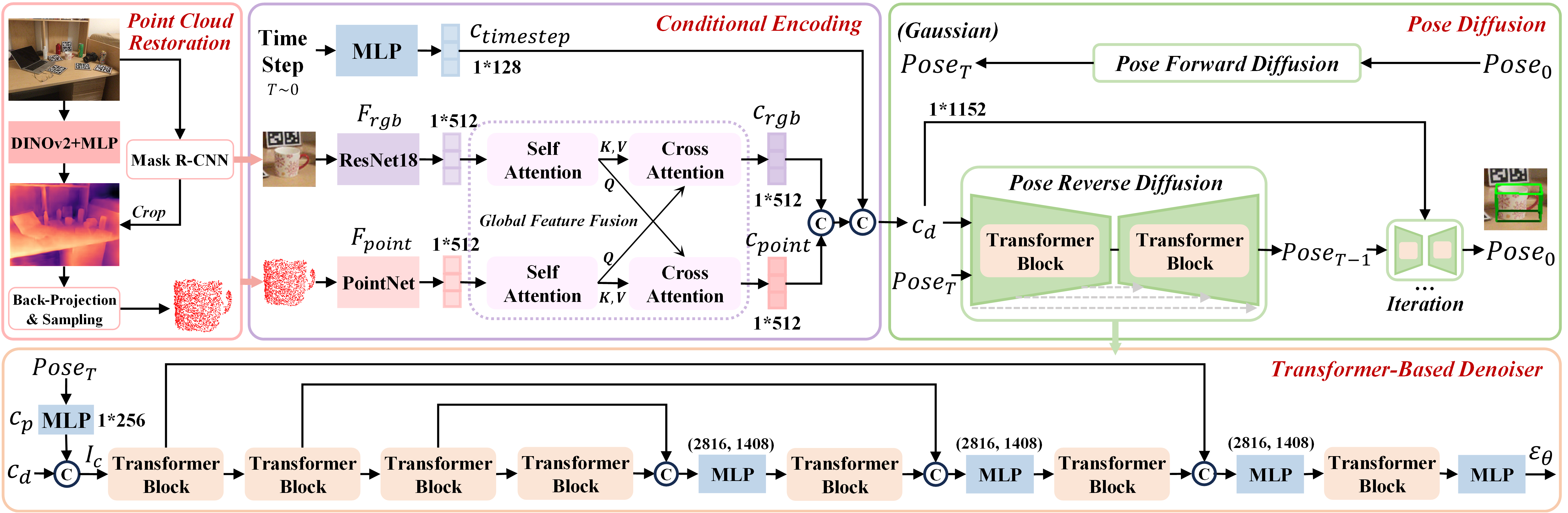
Figure 2 shows an overview of our proposed model. The goal of MonoDiff9D is to predict the 6D pose (composed of 3D translation and 3D rotation) and 3D size (axes lengths of the oriented bounding box) of the intra-class unknown object using only a single RGB image. Given an input RGB image, we first leverage the pre-trained LVM DINOv2 [43] and Mask R-CNN [58] to generate the coarse depth image and segmented RGB image, respectively. The segmented mask is used to crop the coarse depth image. Then, we convert the cropped depth image into a point cloud via back-projection and sampling. Subsequently, we encode all input conditions (including the diffusion time step , RGB image , and restored point cloud as shown in Fig. 2) to provide conditional guidance for accurate reverse diffusion. Specifically, we use MLP to encode the diffusion time step, and leverage the lightweight ResNet18 [59] and PointNet [60] to extract the global features of the observed RGB image and the restored point cloud, respectively. We employ self-attention and cross-attention mechanisms to fuse these two global features. Next, the encoded , , and are concatenated to form the conditional encoding of the diffusion model. Finally, the DDIM [50] is used to denoise the Gaussian noise and recover the actual object pose through a transformer-based denoiser.
III-A Point Cloud Restoration
Point cloud is the most critical input for 9D object pose estimation since it represents the location and geometric information of the observed object. In particular, estimating the 3D object translation from a monocular RGB image is challenging. To introduce the location and geometric information from a single RGB image to condition the learning of the diffusion model, we propose to leverage the pre-trained DINOv2 [43] to perform coarse depth estimation from the RGB image in a zero-shot manner. We elaborate on our choice of using DINOv2 instead of other depth estimators [61, 62] in Sec. IV-D1.
The workflow of the point cloud restoration is shown in Fig. 2. Specifically, we first employ DINOv2 to estimate the coarse depth image corresponding to the observed RGB image. Then, we utilize the Mask R-CNN [58] to perform instance segmentation on the RGB image. Using the segmented mask, we crop the coarse depth image accordingly. Subsequently, the cropped depth image is transformed into a point cloud and downsampled to 1024 points [29, 38].
III-B Conditional Encoding
Adding conditional encoding introduces prompts that make the learning of the diffusion model more accurate [55, 63, 64]. Based on this, taking the time step as an example, we first use MLP to encode the time step . Since the RGB image and point cloud can provide texture and geometric information of the observed object, respectively, these are important inputs for 9D object pose estimation. Conditional encoding of the RGB image and point cloud can effectively make diffusion model learning more robust.
The overall structure of the conditional encoding is shown in Fig. 2. We utilize the lightweight ResNet [59] with the last fully connected layer removed and the PointNet [60] to extract the global features of RGB image and point cloud, respectively. Different from the standard PointNet [60], we only leverage it to extract the global feature as the condition for the efficiency of the diffusion process. Given the disparity between the object point cloud reconstructed using DINOv2 and the actual object point cloud, we utilize self-attention and cross-attention mechanisms to fuse the RGB global feature and the point cloud global feature . This enables our model to pay more attention to the pose-sensitive features of the restored coarse point cloud. The network structures of the self-attention and cross-attention mechanisms are composed of a transformer block, similar to ViT [65]. Their most critical part is the multi-head attention. Taking as an example, it can be expressed as:
| (1) |
where , , and represent query, key, and value, respectively. For self-attention, , , and all come from . For cross-attention, is from , and and are from . denotes the matrix transpose operation. represents the feature dimension of each attention head. denotes first concatenating the feature of all heads, and then feeding the concatenated features to a fully connected layer. Finally, the encoded time step , RGB image , and point cloud are concatenated to form the conditional encoding of the diffusion model as follows:
| (2) |
III-C Pose Diffusion
We leverage the diffusion model because the depth image estimated by DINOv2 [43] may have an error of , and the complete object may not be recovered. When the depth sensors are unavailable, regression-based models such as OLD-Net [46] and DMSR [47] require shape priors and the CAD models of intra-class known objects as additional supervision signals to provide more refined geometric guidance during training. In contrast, diffusion models have strong robustness to recover high-quality outputs from uncertain and noisy conditions [64]. Hence, we do not need to use any shape priors and CAD object models.
The pose diffusion consists of two stages, each characterized as a Markov chain. Specifically, the first stage is forward diffusion, where Gaussian noise with predefined mean and variance is gradually added to the ground-truth object pose. Subsequently, the reverse diffusion stage employs a neural network to progressively denoise Gaussian noise, thus reconstructing the actual object pose.
III-C1 Forward Diffusion
Given a ground-truth object pose , which conforms to the pose distribution , we define a forward diffusion process where Gaussian noise is gradually added to the ground-truth object pose in time steps, producing a sequence of noisy poses . The sequence is controlled by a cosine-schedule and [66]. Following DDPM [57], the step-by-step diffusion process follows the Markov chain assumption:
| (3) |
Specifically, can be defined as:
| (4) |
where is a randomly sampled standard Gaussian noise at time step . Let and and iterate Eq. 4, the forward pose diffusion process from to can be expressed as:
| (5) |
III-C2 Reverse Diffusion
As shown in Fig. 2, the reverse diffusion process aims to recover the actual object pose from a standard Gaussian noise input conditioned on . However, it is difficult to obtain directly, so we run the reverse diffusion process by learning a denoising model to approximate this conditional probability as:
| (6) |
where represents the condition (see Sec. III-B for details). Following DDPM [57] to use Bayes’ theorem transform Eq. 6, then we can get the variance and the mean
| (7) |
Specifically, we first use MLP to encode the input of the diffusion model to obtain the pose feature , and then concatenate it with to form the input of the denoiser as follows:
| (8) |
Since is a one-dimensional vector, we design a transformer-based U-Net as the denoiser. By doing so, each feature channel in can be globally associated with , thus contributing to more robust diffusion. The detailed network structure is shown in Fig. 2. We utilize transformer blocks that are identical to those used in ViT [65].
To improve the running speed of reverse diffusion, we leverage the DDIM scheduler [50] to reduce the number of sampling time steps. Overall, the reverse diffusion aims to estimate the pose noise by learning a neural network conditioned on . Then, we can leverage the DDIM [50] scheduler to denoise, recovering the actual object pose.
III-D Training Protocol
Since can be easily obtained at training time, we use it as the ground truth to supervise the learning of the denoising model. Specifically, the denoising loss term can be parameterized to minimize the difference between and as follows:
| (9) | ||||
IV EXPERIMENTS
IV-A Evaluation Datasets and Metrics
Datasets: We follow previous monocular category-level object pose estimation methods [44, 45, 46, 47] to use the CAMERA25 and REAL275 datasets [26] for evaluation. CAMERA25 is a large synthetic dataset including 1085 instances from 6 categories of objects. REAL275 is a real-world dataset containing 42 instances from the same categories of objects as in CAMERA25. The data split and training mode are identical to the compared methods [44, 45, 46, 47].
| Method | Shape Prior | CAD Model | CAMERA25 | REAL275 | |||||||||||
|---|---|---|---|---|---|---|---|---|---|---|---|---|---|---|---|
|
|
|
|
|
|
|
||||||||||
| Synthesis [44] | - | ✓ | - | - | - | - | - | - | - | 34.0 | 14.2 | 4.8 | |||
| MSOS [45] | - | ✓ | 32.4 | 5.1 | 29.7 | 60.8 | 19.2 | 23.4 | 3.0 | 39.5 | 29.2 | 9.6 | |||
| OLD-Net [46] | ✓ | ✓ | 32.1 | 5.4 | 30.1 | 74.0 | 23.4 | 25.4 | 1.9 | 38.9 | 37.0 | 9.8 | |||
| DMSR [47] | ✓ | ✓ | 34.6 | 6.5 | 32.3 | 81.4 | 27.4 | 28.3 | 6.1 | 37.3 | 59.5 | 23.6 | |||
| MonoDiff9D | - | - | 35.2 | 6.7 | 33.6 | 80.1 | 28.2 | 31.5 | 6.3 | 41.0 | 56.3 | 25.7 | |||
Metrics: Following the comparison methods [44, 45, 46, 47], we choose the widely used and 3D Intersection-over-Union () metrics for evaluation. directly denotes the predicted rotation and translation errors. represents the percentage of intersection and union of the ground-truth and the estimated 3D bounding boxes, which is mainly used to evaluate the size estimation. We follow DMSR [47] to select 50 and 75 as the thresholds of and choose , , and to evaluate the translation and rotation estimation.
IV-B Implementation Details
Since we set the number of attention heads of all the transformer blocks in Fig. 2 to 16 through experiments, the feature dimension in Eq. 1 is set to 32 (calculated by ). The diffusion time step in Eq. 3 is set to 1000. The learning rate is cyclically adjusted between and through the CyclicLR function [67], and the step size of each cycle is set to 20K. We train for 30 cycles, and the batch size of each step is set to 48. Experiments are conducted using a single NVIDIA 3090 GPU. The pose diffusion process achieves a speed of 26.3 frames per second.
IV-C Comparisons with State-of-the-Art Methods
We follow previous SOTA methods [45, 46, 47] to use the CAMERA25 and REAL275 datasets for evaluation. To train and test MonoDiff9D on these two datasets, we extend them with DINOv2 [43] (approximately 276K images) in a zero-shot manner. For a fair comparison, MonoDiff9D and all the comparison methods are provided with the same segmentation results (i.e., segmented by Mask R-CNN [58]).
IV-C1 CAMERA25 Dataset
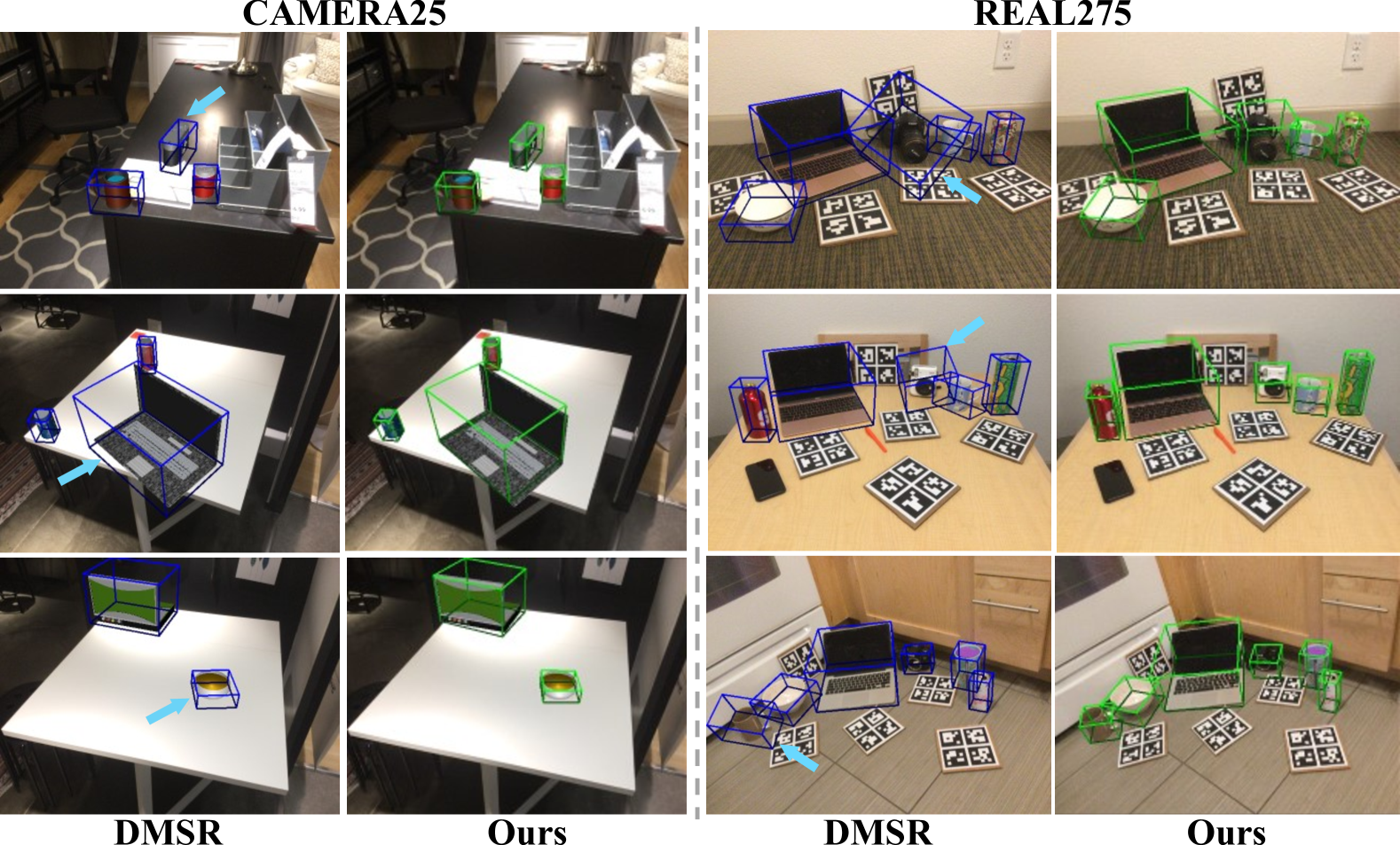
We compare MonoDiff9D with three SOTA methods on the CAMERA25 dataset. The quantitative comparison results are shown in Table I. MonoDiff9D outperforms MSOS [45] and OLD-Net [46] by 19.3 and 6.1 on metric, respectively. Since MSOS [45] lacks the guidance of geometric information, it has lower rotation accuracy. In addition, MonoDiff9D outperforms OLD-Net [46] and DMSR [47] by 4.8 and 0.8 on metric, respectively. It is worth noting that these two comparison methods need to use shape priors and the CAD models of intra-class known objects during training, while MonoDiff9D outperforms them without using these. Some qualitative results are shown in Fig. 3. We can see that MonoDiff9D has a more refined translation and size estimation performance.
| Method |
|
|
|
|||||
|---|---|---|---|---|---|---|---|---|
| DINOv2 + HS-Pose [41] | 19.0 | 1.8 | 27.6 | 42.2 | 12.1 | |||
| DINOv2 + IST-Net [32] | 30.9 | 3.3 | 40.7 | 43.7 | 17.3 | |||
| ZoeDepth + MonoDiff9D | 15.6 | 1.5 | 24.3 | 57.8 | 14.0 | |||
| DINOv2 w/o Diffusion | 21.6 | 2.5 | 30.4 | 52.9 | 19.3 | |||
| DINOv2 + MonoDiff9D | 31.5 | 6.3 | 41.0 | 56.3 | 25.7 |
IV-C2 REAL275 Dataset
We evaluate the performance of our MonoDiff9D on the real-world REAL275 dataset. The quantitative comparison results are shown in Table I. MonoDiff9D outperforms Synthesis [44] and MSOS [45] by 42.1 and 27.1 on metric, respectively. Since both Synthesis [44] and MSOS [45] lack the guidance of geometric information, their rotation estimation accuracy in the real world is much lower than that of methods guided by geometric information. Furthermore, MonoDiff9D outperforms OLD-Net [46] and DMSR [47] by 6.1 and 3.2 on 50 metric, respectively. Note that both OLD-Net [46] and DMSR [47] rely on using shape priors and the CAD models of intra-class known objects during training, which require extensive manual efforts to obtain. MonoDiff9D performs better without using shape priors or CAD models during training. Some qualitative results are shown in Fig. 3. We can see that MonoDiff9D has better size estimation accuracy for some challenging objects (e.g., camera and mug).
IV-D Ablation Studies and Discussions
IV-D1 Depth Estimators and their Suitability for Diffusion Model
First, we take the SOTA category-level 9D object pose estimation methods HS-Pose (depth-based) [41] and IST-Net (RGBD-based) [32] and replace their depth data with that restored by DINOv2 [43] during training as well as inference while keeping all other experimental settings unchanged. Detailed results are shown in Table II. We can see that both HS-Pose and IST-Net do not perform well since the depth images from DINOv2 contain an error of and the complete object is not always restored. Our method is more robust to uncertain and noisy conditions. Additionally, other depth estimators have been proposed recently, such as Depth Anything [61] and ZoeDepth [62]. Depth Anything mainly estimates the relative depth and does not perform metric depth estimation which is required by our model. Hence, we choose ZoeDepth for ablation study (i.e., the depth during training and inference is restored with ZoeDepth). Experimental results demonstrate that DINOv2 outperforms ZoeDepth. It is worth noting that ZoeDepth is specifically designed for monocular depth estimation, while DINOv2 is not. We believe that DINOv2 performs better because its extensive and powerful self-supervised pre-training allows it to better extract semantically consistent features. Moreover, we eliminate the diffusion model and retain the same network as the denoiser for feature fusion, followed by using fully connected layers to regress , , and individually. The significant decline in all metrics demonstrates the effectiveness of the diffusion model.
| Row |
|
|
|
|||||||||
|---|---|---|---|---|---|---|---|---|---|---|---|---|
| 1 | - | ✓ | ✓ | ✓ | 29.5 | 5.3 | 36.2 | 56.0 | 21.6 | |||
| 2 | ✓ | - | ✓ | ✓ | 1.5 | 0.0 | 4.0 | 16.2 | 0.6 | |||
| 3 | ✓ | ✓ | - | - | 28.6 | 4.8 | 34.9 | 55.5 | 21.7 | |||
| 4 | ✓ | ✓ | - | ✓ | 27.7 | 4.5 | 35.9 | 56.2 | 22.6 | |||
| 5 | ✓ | ✓ | ✓ | - | 30.9 | 6.0 | 39.5 | 57.1 | 25.0 | |||
| 6 | ✓ | ✓ | ✓ | * | 31.3 | 5.2 | 40.1 | 57.3 | 25.6 | |||
| 7 | ✓ | ✓ | ✓ | ✓ | 31.5 | 6.3 | 41.0 | 56.3 | 25.7 |
IV-D2 Conditional Encoding
We remove the global feature fusion module and the conditional encoding of the time step, respectively, to explore their contribution to MonoDiff9D.
Global Feature Fusion (): Compared with the original MonoDiff9D, the 50 and 75 metrics drop by 2.0 and 1.0, respectively. The quantitative results are shown in the first row of Table III. These results show that the global feature fusion module in the conditional encoding part enhances the accuracy of MonoDiff9D. Specifically, it helps MonoDiff9D pay more attention to pose-sensitive information from the restored coarse point cloud.
Time Step (): We remove the conditional encoding of the time step and keep the other encoding part unchanged. The quantitative results are shown in the second row of Table III. The metric drops from 41.0 to 4.0, and the metric drops from 56.3 to 16.2. These results show that the conditional encoding of the time step is significant for the diffusion model. Since the noise-adding amplitude of the diffusion model correlates with the time step, incorporating time information via conditional encoding can enhance the robustness of the diffusion model learning process.
IV-D3 Denoiser
For the diffusion process, we conduct ablation studies on the transformer-based denoiser of the reverse diffusion process to justify its design.
Transformer Block (): To prove the applicability of transformer to pose diffusion, we replace the transformer blocks with MLPs and remove the skip concatenation in the denoiser. The and metrics drop by 6.1 and 0.8, respectively. When adding the skip concatenation, the metric still drops by 3.1. These results are shown in the third and fourth rows of Table III, which show that the transformer blocks contribute to improving the accuracy of MonoDiff9D. Since the input of the denoiser is a one-dimensional vector, each feature channel in can be globally associated with the condition via the transformer blocks, thus contributing to more precise diffusion.
| Method |
|
|
|
|||||
|---|---|---|---|---|---|---|---|---|
| DINOv2 + HS-Pose [41] | 8.5 | 0.2 | 33.2 | 11.4 | 3.4 | |||
| DINOv2 + IST-Net [32] | 3.1 | 0.0 | 26.0 | 15.5 | 7.4 | |||
| DINOv2 + MonoDiff9D | 9.6 | 0.4 | 36.3 | 23.4 | 11.1 |
Skip Concatenation (): We first remove it directly to demonstrate the effectiveness of skip concatenation in the denoiser. The quantitative results are shown in the fifth row of Table III. Compared with the original MonoDiff9D, the metric drops by 0.7. Moreover, we use the common residual connection instead of concatenation. The quantitative results are shown in the sixth row of Table III. The the 75 metric drops by 1.1. These results show that skip concatenation in the denoiser is important. Since the skip concatenation can retain more spatial information, it is significant for the reverse diffusion process.
IV-D4 Generalization in the Wild
We use only the test set of the Wild6D [36] dataset to investigate the generalization ability of MonoDiff9D to images in the wild. Wild6D is a large dataset collected in diverse environments, which includes annotations for 486 test videos featuring various backgrounds and 162 instances. It is worth noting that the Wild6D dataset is mainly used to evaluate self-supervised methods, and its training set has no labels, so we do not train on this dataset. Since current monocular methods either have unavailable codes and models [44, 45, 46] or require 2.5D sketches as additional input [47], we use our MonoDiff9D, HS-Pose [41], and IST-Net [32] to perform ablation studies. Detailed results are shown in Table IV. This experiment demonstrates that MonoDiff9D has better generalization ability in the wild than HS-Pose [41] and IST-Net [32]. We believe that this advantage mainly comes from the extensive sampling on the Markov chain of our diffusion-based framework, which can effectively expand the data distribution.
V CONCLUSIONS
This paper presented MonoDiff9D, a diffusion-based method for monocular category-level 9D object pose estimation. We leveraged the probabilistic nature of the diffusion model and the LVM DINOv2 to enhance intra-class unknown object pose estimation when shape priors, CAD models, and depth sensors are unavailable. Extensive experiments demonstrate that MonoDiff9D achieves SOTA accuracy. Future work can use the features of the RGB image to enhance the refinement of the coarse depth map generated by DINOv2. Additionally, exploring the integration of more advanced LVMs could also lead to improved performance in the wild.
Acknowledgments: This work was supported by the National Natural Science Foundation of China under Grant U22A2059 and Grant 62473141, China Scholarship Council under Grant 202306130074, and Natural Science Foundation of Hunan Province under Grant 2024JJ5098.
References
- [1] Y. Liu, Y. Wen, S. Peng, C. Lin, X. Long, T. Komura, and W. Wang, “Gen6d: Generalizable model-free 6-dof object pose estimation from rgb images,” in European Conference on Computer Vision, 2022, pp. 298–315.
- [2] J. Liu, W. Sun, C. Liu, X. Zhang, and Q. Fu, “Robotic continuous grasping system by shape transformer-guided multi-object category-level 6-d pose estimation,” IEEE Transactions on Industrial Informatics, vol. 19, no. 11, pp. 11 171–11 181, 2023.
- [3] V. N. Nguyen, T. Groueix, M. Salzmann, and V. Lepetit, “Gigapose: Fast and robust novel object pose estimation via one correspondence,” in Proceedings of the IEEE/CVF Conference on Computer Vision and Pattern Recognition, 2024, pp. 9903–9913.
- [4] C. Liu, W. Sun, J. Liu, X. Zhang, S. Fan, and Q. Fu, “Fine segmentation and difference-aware shape adjustment for category-level 6dof object pose estimation,” Applied Intelligence, vol. 53, no. 20, pp. 23 711–23 728, 2023.
- [5] J. Cai, Y. He, W. Yuan, S. Zhu, Z. Dong, L. Bo, and Q. Chen, “Open-vocabulary category-level object pose and size estimation,” IEEE Robotics and Automation Letters, vol. 9, no. 9, pp. 7661–7668, 2024.
- [6] J. Liu, W. Sun, H. Yang, Z. Zeng, C. Liu, J. Zheng, X. Liu, H. Rahmani, N. Sebe, and A. Mian, “Deep learning-based object pose estimation: a comprehensive survey,” arXiv preprint arXiv:2405.07801, 2024.
- [7] F. Manhardt, W. Kehl, and A. Gaidon, “Roi-10d: Monocular lifting of 2d detection to 6d pose and metric shape,” in Proceedings of the IEEE/CVF Conference on Computer Vision and Pattern Recognition, 2019, pp. 2069–2078.
- [8] B. Fu, S. K. Leong, X. Lian, and X. Ji, “6d robotic assembly based on rgb-only object pose estimation,” in IEEE/RSJ International Conference on Intelligent Robots and Systems, 2022, pp. 4736–4742.
- [9] A. Remus, S. D’Avella, F. Di Felice, P. Tripicchio, and C. A. Avizzano, “i2c-net: using instance-level neural networks for monocular category-level 6d pose estimation,” IEEE Robotics and Automation Letters, vol. 8, no. 3, pp. 1515–1522, 2023.
- [10] V. N. Nguyen, T. Groueix, G. Ponimatkin, Y. Hu, R. Marlet, M. Salzmann, and V. Lepetit, “Nope: Novel object pose estimation from a single image,” in Proceedings of the IEEE/CVF Conference on Computer Vision and Pattern Recognition, 2024, pp. 17 923–17 932.
- [11] Z. Li, X. Xu, S. Lim, and H. Zhao, “Unimode: Unified monocular 3d object detection,” in Proceedings of the IEEE/CVF Conference on Computer Vision and Pattern Recognition, 2024, pp. 16 561–16 570.
- [12] J. Liu, W. Sun, H. Yang, C. Liu, X. Zhang, and A. Mian, “Domain-generalized robotic picking via contrastive learning-based 6-d pose estimation,” IEEE Transactions on Industrial Informatics, vol. 20, no. 6, pp. 8650–8661, 2024.
- [13] S. Peng, X. Zhou, Y. Liu, H. Lin, Q. Huang, and H. Bao, “Pvnet: Pixel-wise voting network for 6dof object pose estimation,” IEEE Transactions on Pattern Analysis and Machine Intelligence, vol. 44, no. 6, pp. 3212–3223, 2022.
- [14] Y. He, W. Sun, H. Huang, J. Liu, H. Fan, and J. Sun, “Pvn3d: A deep point-wise 3d keypoints voting network for 6dof pose estimation,” in Proceedings of the IEEE/CVF Conference on Computer Vision and Pattern Recognition, 2020, pp. 11 632–11 641.
- [15] C. Wang, D. Xu, Y. Zhu, R. Martín-Martín, C. Lu, L. Fei-Fei, and S. Savarese, “Densefusion: 6d object pose estimation by iterative dense fusion,” in Proceedings of the IEEE/CVF Conference on Computer Vision and Pattern Recognition, 2019, pp. 3343–3352.
- [16] Y. He, H. Huang, H. Fan, Q. Chen, and J. Sun, “Ffb6d: A full flow bidirectional fusion network for 6d pose estimation,” in Proceedings of the IEEE/CVF Conference on Computer Vision and Pattern Recognition, 2021, pp. 3003–3013.
- [17] G. Wang, F. Manhardt, F. Tombari, and X. Ji, “Gdr-net: Geometry-guided direct regression network for monocular 6d object pose estimation,” in Proceedings of the IEEE/CVF Conference on Computer Vision and Pattern Recognition, 2021, pp. 16 611–16 621.
- [18] J. Liu, W. Sun, C. Liu, X. Zhang, S. Fan, and W. Wu, “Hff6d: Hierarchical feature fusion network for robust 6d object pose tracking,” IEEE Transactions on Circuits and Systems for Video Technology, vol. 32, no. 11, pp. 7719–7731, 2022.
- [19] Y. Weng, H. Wang, Q. Zhou, Y. Qin, Y. Duan, Q. Fan, B. Chen, H. Su, and L. J. Guibas, “Captra: Category-level pose tracking for rigid and articulated objects from point clouds,” in Proceedings of the IEEE/CVF International Conference on Computer Vision, 2021, pp. 13 209–13 218.
- [20] B. Wen and K. Bekris, “Bundletrack: 6d pose tracking for novel objects without instance or category-level 3d models,” in IEEE/RSJ International Conference on Intelligent Robots and Systems, 2021, pp. 8067–8074.
- [21] J. Liu, W. Sun, C. Liu, H. Yang, X. Zhang, and A. Mian, “Mh6d: Multi-hypothesis consistency learning for category-level 6-d object pose estimation,” IEEE Transactions on Neural Networks and Learning Systems., pp. 1–14, 2024.
- [22] J. Wang, K. Chen, and Q. Dou, “Category-level 6d object pose estimation via cascaded relation and recurrent reconstruction networks,” in Proceedings of the IEEE/RSJ International Conference on Intelligent Robots and Systems, 2021, pp. 4807–4814.
- [23] P. Wang, H. Jung, Y. Li, S. Shen, R. P. Srikanth, L. Garattoni, S. Meier, N. Navab, and B. Busam, “Phocal: A multi-modal dataset for category-level object pose estimation with photometrically challenging objects,” in Proceedings of the IEEE/CVF Conference on Computer Vision and Pattern Recognition, 2022, pp. 21 222–21 231.
- [24] H. Jung, S.-C. Wu, P. Ruhkamp, G. Zhai, H. Schieber, G. Rizzoli, P. Wang, H. Zhao, L. Garattoni, S. Meier et al., “Housecat6d–a large-scale multi-modal category level 6d object pose dataset with household objects in realistic scenarios,” in Proceedings of the IEEE/CVF Conference on Computer Vision and Pattern Recognition, 2024, pp. 22 498–22 508.
- [25] X. Lin, W. Yang, Y. Gao, and T. Zhang, “Instance-adaptive and geometric-aware keypoint learning for category-level 6d object pose estimation,” in Proceedings of the IEEE/CVF Conference on Computer Vision and Pattern Recognition, 2024, pp. 21 040–21 049.
- [26] H. Wang, S. Sridhar, J. Huang, J. Valentin, S. Song, and L. J. Guibas, “Normalized object coordinate space for category-level 6d object pose and size estimation,” in Proceedings of the IEEE/CVF Conference on Computer Vision and Pattern Recognition, 2019, pp. 2642–2651.
- [27] S. Umeyama, “Least-squares estimation of transformation parameters between two point patterns,” IEEE Transactions on Pattern Analysis and Machine Intelligence, vol. 13, no. 04, pp. 376–380, 1991.
- [28] M. Tian, M. H. Ang, and G. H. Lee, “Shape prior deformation for categorical 6d object pose and size estimation,” in European Conference on Computer Vision, 2020, pp. 530–546.
- [29] K. Chen and Q. Dou, “Sgpa: Structure-guided prior adaptation for category-level 6d object pose estimation,” in Proceedings of the IEEE/CVF International Conference on Computer Vision, 2021, pp. 2773–2782.
- [30] R. Zhang, Y. Di, F. Manhardt, F. Tombari, and X. Ji, “Ssp-pose: Symmetry-aware shape prior deformation for direct category-level object pose estimation,” in Proceedings of the IEEE/RSJ International Conference on Intelligent Robots and Systems, 2022, pp. 7452–7459.
- [31] J. Lin, Z. Wei, Z. Li, S. Xu, K. Jia, and Y. Li, “Dualposenet: Category-level 6d object pose and size estimation using dual pose network with refined learning of pose consistency,” in Proceedings of the IEEE/CVF International Conference on Computer Vision, 2021, pp. 3560–3569.
- [32] J. Liu, Y. Chen, X. Ye, and X. Qi, “Ist-net: Prior-free category-level pose estimation with implicit space transformation,” in Proceedings of the IEEE/CVF International Conference on Computer Vision, 2023, pp. 13 978–13 988.
- [33] J. Lin, Z. Wei, Y. Zhang, and K. Jia, “Vi-net: Boosting category-level 6d object pose estimation via learning decoupled rotations on the spherical representations,” in Proceedings of the IEEE/CVF International Conference on Computer Vision, 2023, pp. 14 001–14 011.
- [34] W. Peng, J. Yan, H. Wen, and Y. Sun, “Self-supervised category-level 6d object pose estimation with deep implicit shape representation,” in Proceedings of the AAAI Conference on Artificial Intelligence, vol. 36, no. 2, 2022, pp. 2082–2090.
- [35] T. Lee, B.-U. Lee, I. Shin, J. Choe, U. Shin, I. S. Kweon, and K.-J. Yoon, “Uda-cope: unsupervised domain adaptation for category-level object pose estimation,” in Proceedings of the IEEE/CVF Conference on Computer Vision and Pattern Recognition, 2022, pp. 14 891–14 900.
- [36] Y. Ze and X. Wang, “Category-level 6d object pose estimation in the wild: A semi-supervised learning approach and a new dataset,” in Advances in Neural Information Processing Systems, vol. 35, 2022, pp. 27 469–27 483.
- [37] T. Lee, J. Tremblay, V. Blukis, B. Wen, B.-U. Lee, I. Shin, S. Birchfield, I. S. Kweon, and K.-J. Yoon, “Tta-cope: Test-time adaptation for category-level object pose estimation,” in Proceedings of the IEEE/CVF Conference on Computer Vision and Pattern Recognition, 2023, pp. 21 285–21 295.
- [38] J. Lin, Z. Wei, C. Ding, and K. Jia, “Category-level 6d object pose and size estimation using self-supervised deep prior deformation networks,” in European Conference on Computer Vision, 2022, pp. 19–34.
- [39] W. Chen, X. Jia, H. J. Chang, J. Duan, L. Shen, and A. Leonardis, “Fs-net: Fast shape-based network for category-level 6d object pose estimation with decoupled rotation mechanism,” in Proceedings of the IEEE/CVF Conference on Computer Vision and Pattern Recognition, 2021, pp. 1581–1590.
- [40] Y. Di, R. Zhang, Z. Lou, F. Manhardt, X. Ji, N. Navab, and F. Tombari, “Gpv-pose: Category-level object pose estimation via geometry-guided point-wise voting,” in Proceedings of the IEEE/CVF Conference on Computer Vision and Pattern Recognition, 2022, pp. 6781–6791.
- [41] L. Zheng, C. Wang, Y. Sun, E. Dasgupta, H. Chen, A. Leonardis, W. Zhang, and H. J. Chang, “Hs-pose: Hybrid scope feature extraction for category-level object pose estimation,” in Proceedings of the IEEE/CVF Conference on Computer Vision and Pattern Recognition, 2023, pp. 17 163–17 173.
- [42] H. Lin, Z. Liu, C. Cheang, Y. Fu, G. Guo, and X. Xue, “Sar-net: Shape alignment and recovery network for category-level 6d object pose and size estimation,” in Proceedings of the IEEE/CVF Conference on Computer Vision and Pattern Recognition, 2022, pp. 6707–6717.
- [43] M. Oquab, T. Darcet, T. Moutakanni, H. Vo, M. Szafraniec, V. Khalidov, P. Fernandez, D. Haziza, F. Massa, A. El-Nouby et al., “Dinov2: Learning robust visual features without supervision,” arXiv preprint arXiv:2304.07193, 2023.
- [44] X. Chen, Z. Dong, J. Song, A. Geiger, and O. Hilliges, “Category level object pose estimation via neural analysis-by-synthesis,” in European Conference on Computer Vision, 2020, pp. 139–156.
- [45] T. Lee, B.-U. Lee, M. Kim, and I. S. Kweon, “Category-level metric scale object shape and pose estimation,” IEEE Robotics and Automation Letters, vol. 6, no. 4, pp. 8575–8582, 2021.
- [46] Z. Fan, Z. Song, J. Xu, Z. Wang, K. Wu, H. Liu, and J. He, “Object level depth reconstruction for category level 6d object pose estimation from monocular rgb image,” in European Conference on Computer Vision, 2022, pp. 220–236.
- [47] J. Wei, X. Song, W. Liu, L. Kneip, H. Li, and P. Ji, “Rgb-based category-level object pose estimation via decoupled metric scale recovery,” in IEEE International Conference on Robotics and Automation, 2024, pp. 2036–2042.
- [48] F. Manhardt, G. Wang, B. Busam, M. Nickel, S. Meier, L. Minciullo, X. Ji, and N. Navab, “Cps++: Improving class-level 6d pose and shape estimation from monocular images with self-supervised learning,” arXiv preprint arXiv:2003.05848, 2020.
- [49] J. Liu, W. Sun, H. Yang, P. Deng, C. Liu, N. Sebe, H. Rahmani, and A. Mian, “Diff9d: Diffusion-based domain-generalized category-level 9-dof object pose estimation,” arXiv preprint arXiv:2502.02525, 2025.
- [50] J. Song, C. Meng, and S. Ermon, “Denoising diffusion implicit models,” in International Conference on Learning Representations, 2020.
- [51] M. Z. Irshad, T. Kollar, M. Laskey, K. Stone, and Z. Kira, “Centersnap: Single-shot multi-object 3d shape reconstruction and categorical 6d pose and size estimation,” in International Conference on Robotics and Automation, 2022, pp. 10 632–10 640.
- [52] M. Lunayach, S. Zakharov, D. Chen, R. Ambrus, Z. Kira, and M. Z. Irshad, “Fsd: Fast self-supervised single rgb-d to categorical 3d objects,” in IEEE International Conference on Robotics and Automation, 2024, pp. 14 630–14 637.
- [53] T. Ikeda, S. Zakharov, T. Ko, M. Z. Irshad, R. Lee, K. Liu, R. Ambrus, and K. Nishiwaki, “Diffusionnocs: Managing symmetry and uncertainty in sim2real multi-modal category-level pose estimation,” arXiv preprint arXiv:2402.12647, 2024.
- [54] Y. You, R. Shi, W. Wang, and C. Lu, “Cppf: Towards robust category-level 9d pose estimation in the wild,” in Proceedings of the IEEE/CVF Conference on Computer Vision and Pattern Recognition, 2022, pp. 6866–6875.
- [55] J. Zhang, M. Wu, and H. Dong, “Generative category-level object pose estimation via diffusion models,” in Advances in Neural Information Processing Systems, vol. 36, 2023, pp. 1–14.
- [56] Y. Lin, J. Tremblay, S. Tyree, P. A. Vela, and S. Birchfield, “Single-stage keypoint-based category-level object pose estimation from an rgb image,” in International Conference on Robotics and Automation, 2022, pp. 1547–1553.
- [57] J. Ho, A. Jain, and P. Abbeel, “Denoising diffusion probabilistic models,” in Advances in Neural Information Processing Systems, vol. 33, 2020, pp. 6840–6851.
- [58] K. He, G. Gkioxari, P. Dollár, and R. Girshick, “Mask r-cnn,” in Proceedings of the IEEE International Conference on Computer Vision, 2017, pp. 2961–2969.
- [59] K. He, X. Zhang, S. Ren, and J. Sun, “Deep residual learning for image recognition,” in Proceedings of the IEEE/CVF Conference on Computer Vision and Pattern Recognition, 2016, pp. 770–778.
- [60] C. R. Qi, H. Su, K. Mo, and L. J. Guibas, “Pointnet: Deep learning on point sets for 3d classification and segmentation,” in Proceedings of the IEEE/CVF Conference on Computer Vision and Pattern Recognition, 2017, pp. 652–660.
- [61] L. Yang, B. Kang, Z. Huang, X. Xu, J. Feng, and H. Zhao, “Depth anything: Unleashing the power of large-scale unlabeled data,” in Proceedings of the IEEE/CVF Conference on Computer Vision and Pattern Recognition, 2024, pp. 10 371–10 381.
- [62] S. F. Bhat, R. Birkl, D. Wofk, P. Wonka, and M. Müller, “Zoedepth: Zero-shot transfer by combining relative and metric depth,” arXiv preprint arXiv:2302.12288, 2023.
- [63] J. Gong, L. G. Foo, Z. Fan, Q. Ke, H. Rahmani, and J. Liu, “Diffpose: Toward more reliable 3d pose estimation,” in Proceedings of the IEEE/CVF Conference on Computer Vision and Pattern Recognition, 2023, pp. 13 041–13 051.
- [64] R. Rombach, A. Blattmann, D. Lorenz, P. Esser, and B. Ommer, “High-resolution image synthesis with latent diffusion models,” in Proceedings of the IEEE/CVF Conference on Computer Vision and Pattern Recognition, 2022, pp. 10 684–10 695.
- [65] A. Dosovitskiy, L. Beyer, A. Kolesnikov, D. Weissenborn, X. Zhai, T. Unterthiner, M. Dehghani, M. Minderer, G. Heigold, S. Gelly et al., “An image is worth 16x16 words: Transformers for image recognition at scale,” in International Conference on Learning Representations, 2020.
- [66] A. Q. Nichol and P. Dhariwal, “Improved denoising diffusion probabilistic models,” in International Conference on Machine Learning, 2021, pp. 8162–8171.
- [67] L. N. Smith, “Cyclical learning rates for training neural networks,” in 2017 IEEE Winter Conference on Applications of Computer Vision, 2017, pp. 464–472.