Software package for simulations using the coarse-grained CALVADOS model

Abstract

We present the CALVADOS package for performing simulations of biomolecules using OpenMM and the coarse-grained CALVADOS model. The package makes it easy to run simulations using the family of CALVADOS models of biomolecules including disordered proteins, multi-domain proteins, proteins in crowded environments, and disordered RNA. We briefly describe the CALVADOS force fields and how they were parametrised. We then discuss the design paradigms and architecture of the CALVADOS package, and give examples of how to use it for running and analysing simulations. The simulation package is freely available under a GNU GPL license; therefore, it can easily be extended and we provide some examples of how this might be done.

Structural Biology and NMR Laboratory, Linderstrøm-Lang Centre for Protein Science, Department of Biology, University of Copenhagen, Copenhagen, Denmark Contributed equally to this work, listed in random order Contributed equally to this work, listed in random order Contributed equally to this work, listed in random order Contributed equally to this work, listed in random order Contributed equally to this work, listed in random order Contributed equally to this work, listed in random order

1 Introduction

1.1 Coarse-grained molecular models for simulations of disordered and multi-domain biomolecules

Intrinsically disordered proteins and regions in proteins (IDPs and IDRs) are important for biological function and involved in various diseases ¹. Around 30% of the residues in the human proteome are predicted to be disordered with around 70% of human proteins containing at least one long (>30 residues) IDR, and some proteins are fully disordered in vitro and in the cell ¹, ², ³. IDRs adopt broad sets of interconverting configurations, and the properties of such conformational ensembles are modulated by the amino acid sequence and solution conditions, and influence phase behaviour and protein function in the cell ¹.

Molecular dynamics (MD) simulations can be used to examine the behaviour of biomolecules at high spatial and temporal resolution. MD simulations numerically integrate a set of equations of motion using interaction potentials (force fields) that are typically parametrised using a combination of experimental data and higher-level (for example quantum-chemical) calculations. Historically, disordered proteins are difficult targets for atomistic molecular simulations. This difficulty arises from two main challenges: The force field problem and the sampling problem. Force fields for atomistic biomolecular simulations were originally mostly tested to model short peptides or the folded states of proteins, and were later found to give rise to unphysically compact IDR ensembles and overly attractive protein-protein interactions ⁴. Several more modern force fields can describe both folded and disordered proteins relatively well ⁵, ⁶, ⁷. However, some inaccuracies persist, including in capturing the global chain dimensions, which vary significantly with the choice of water model ⁸. The sampling problem relates to the challenge of exhaustively sampling protein conformational states. For a simulation of a protein in explicit solvent, most computational resources are spent on calculating water interactions. This is exacerbated by the large simulation boxes needed to minimise finite-size effects in simulations of disordered molecules with extended conformations that might interact across periodic images.

One approach to enhance sampling of conformational space is to simplify the description of the protein, water, or both. Below we describe some of these models that have been applied to IDPs, but do not intend to provide a comprehensive overview of the many models that are available. In models such as ABSINTH ⁹, PROFASI ¹⁰ and CHARMM EEF1 ¹¹, ¹² the protein is described in atomistic detail, but with a continuum model for the solvent. In models such as Martini ¹³, SPICA ¹⁴ and SIRAH ¹⁵ both protein and water molecules are described with a coarse-grained representation, and updated versions have been described that better capture larger-scale conformational properties of IDPs ¹⁶, ¹⁷, ¹⁸, ¹⁹, ²⁰. Despite the reduced number of particles and allowing for larger time steps in MD, these force fields can still be computationally demanding, both for large systems and for single-chain simulations of long IDPs.

A set of models coarse-grain even further by combining a coarse-grained model of the protein with a continuum representation of the solvent. Several of these represent the protein by two or more beads per residue and have been applied to study IDPs ²¹, ²², ²³. Here we instead focus on models where residues are mapped onto single beads ²⁴, ²⁵, ²⁶, ²⁷, ²⁸, ²⁹, ³⁰, ³¹, ³²; we note that several other such models exist. We here refer to these as hydrophobicity scale (HPS) models, although the term HPS was originally meant to indicate a specific set of parameters in one such model ²⁷. In HPS models, the solvent is treated implicitly as a dielectric continuum. To account for water-mediated interactions, the pairwise potentials between residues are scaled according to their hydropathy or ‘stickiness’, as defined by a hydrophobicity scale. Various HPS models have been developed, differing in the hydrophobicity scale used, the treatment of charges ³³, and the use of additional interaction terms like dihedral angle potentials ³⁴.

Simulations with HPS models are computationally efficient enough to be applied to study conformational properties of thousands of isolated IDRs at the proteome scale ³⁵, ³⁶, to perform hundreds of simulations one after another ³⁷, and to simulate hundreds of chains to predict the propensity of proteins to undergo phase separation ²⁷, ³⁸, ³⁹, ⁴⁰, ⁴¹. As such, simulations with HPS models have also been used to train or benchmark models that predict biophysical properties of IDRs from their sequence ⁴², ³⁶, ³⁵, ⁴³, ⁴⁴ and deep learning models that generate conformational ensembles directly from sequence ⁴⁵, ⁴⁶, ⁴⁷, ⁴⁸, ⁴⁹.

HPS models were originally designed and tested for disordered proteins, but have also been applied or tested more extensively to study multi-domain proteins (MDPs), consisting of folded domains connected by flexible linkers ²⁷, ⁵⁰, ⁵¹, ³², and to disordered single-stranded RNA ⁵², ³¹, ⁵³, ⁵⁴.

1.2 The CALVADOS force fields

We have developed a set of CALVADOS (Coarse-graining Approach to Liquid-liquid phase separation Via an Automated Data-driven Optimisation Scheme) models for simulations of proteins and other molecules. Here, we briefly describe the general pair potentials of this family of HPS models, which include the CALVADOS 2 force field for IDRs ²⁹, ⁴⁰ and its extensions to MDPs (CALVADOS 3) ⁵¹, RNA ⁵⁴, and PEG ⁵⁵. Further details on molecule-specific interactions are covered in the next section.

Bonds between residues are described by a harmonic potential,

$$u_{\text{bond}}(r)=\frac{1}{2}k(r-r_{0})^{2},$$ (1)

where $k=$8033\text{\,}\mathrm{k}\mathrm{J}\mathrm{mol}^{-1}\mathrm{n}\mathrm{m}^{-2}$$ is the force constant and $r_{0}$ is the molecule-specific equilibrium bond distance.

Nonbonded non-ionic interactions are described by the Ashbaugh-Hatch (AH) potential ²⁴, a modified Lennard-Jones (LJ) potential that effectively accounts for any non-ionic interaction, such as hydrophobic interactions, $\pi$-$\pi$ stacking, and hydrogen bonding. Key parameters of this potential are the amino acid-specific diameters, $\sigma$, and stickiness values, $\lambda$, which together influence the strength and the range of the interaction. In CALVADOS, the AH potential is truncated and shifted at $r_{c,\text{AH}}=2$ nm ⁴⁰,

$$u_{\text{AH}}(r)=\left\{\begin{aligned} &u_{\text{LJ}}(r)-{\lambda}u_{\text{LJ}}(r_{c,\text{AH}})+{\epsilon}(1-\lambda),&r\leq 2^{1/6}\sigma\\ &{\lambda}[u_{\text{LJ}}(r)-u_{\text{LJ}}(r_{c,\text{AH}})],&2^{1/6}\sigma<r\leq r_{c,\text{AH}}\\ &0,&r>r_{c,\text{AH}}\end{aligned}\right.$$ (2)

where $\sigma=(\sigma_{i}+\sigma_{j})/2$, $\lambda=(\lambda_{i}+\lambda_{j})/2$ for residues $i$ and $j$, and the classic LJ potential,

$$u_{\text{LJ}}(r)=4{\epsilon}\left[\left(\frac{\sigma}{r}\right)^{12}-\left(\frac{\sigma}{r}\right)^{6}\right],$$ (3)

with ${\epsilon}=$0.8368\text{\,}\mathrm{kJ}\text{\,}{\mathrm{mol}}^{-1}$$.

The $\lambda$ parameters are key ingredients in the CALVADOS force field, as they capture the effective interactions between amino acid residues. We have developed an approach to learn force field parameters from experimental data ²⁵ and used similar procedures to learn the $\lambda$ values in the CALVADOS protein force fields ²⁹, ⁴⁰, ⁵¹.

Solvent-mediated salt-screened charge-charge (ionic) interactions are modelled via the Debye-Hückel (DH) potential, truncated and shifted at $r_{c,\text{DH}}=4$ nm,

$$u_{\text{DH}}(r)=\left\{\begin{aligned} &\frac{Z_{i}Z_{j}e^{2}}{4\pi\epsilon_{0}\epsilon_{r}}\left[\frac{\exp(-r/D)}{r}-\frac{\exp(-r_{c,\text{DH}}/D)}{r_{c,\text{DH}}}\right],&r\leq r_{c,\text{DH}}\\ &0,&r>r_{c,\text{DH}},\end{aligned}\right.$$ (4)

Here, $e$ is the elementary charge, $Z_{i}$ and $Z_{j}$ are the charge numbers of beads $i$ and $j$, $\epsilon_{0}$ is the vacuum permittivity, $D=\sqrt{1/(8{\pi}BI)}$ is the Debye length of an electrolyte solution of ionic strength $I$, and $B({\epsilon}_{r})$ is the Bjerrum length of the temperature-dependent dielectric constant $\epsilon_{r}$ ⁵⁶,

$$\begin{split}{\epsilon}_{r}(T)=\frac{5321}{T}&+233.76-0.9297\,T\\ &+1.417{\times}10^{-3}\,T^{2}-8.292{\times}10^{-7}\,T^{3}.\end{split}$$ (5)

To model the effect of different solution pH values, we set the charge of the histidine residues using the Henderson-Hasselbalch equation,

$$Z_{\text{His}}=\frac{1}{1+10^{\text{pH}-\text{p}K_{a}}},$$ (6)

with $\text{p}K_{a}=6.00$.

1.3 Additional molecule-specific CALVADOS parametrization

The details of the models describing folded protein domains, disordered RNA and polyethylene glycol (PEG) crowding have been described in detail before ⁵¹, ⁵⁴, ⁵⁵ and will only be summarized here.

Briefly, folded domains are manually restrained using a harmonic potential between nonbonded pairs of residues within a cutoff of $0.9\text{\,}\mathrm{nm}$. The equilibrium distance of such a restraint is set to the centre-of-mass (COM) separation calculated from a structure that is used as input. For MDPs consisting of folded domains connected by IDRs, we showed that the COM representation reduces overly attractive domain–domain interactions and thereby prevents the compact ensembles observed for some proteins when using the C_α representation ⁵¹. Therefore, we use a mixed representation for MDPs, where residues in folded domains are represented by their COMs and those in IDRs by their C_α atoms, using the same C_α-C_α equilibrium distance of $0.38\text{\,}\mathrm{nm}$ as for the CALVADOS 2 force field. Using this mapping, we reoptimised the $\lambda$ parameters of the model and obtained CALVADOS 3, which performs on par with CALVADOS 2 for IDPs while improving the model accuracy for MDPs.

Synthetic crowders are often used to probe the effect of nonspecific macromolecular crowding on the dynamics of proteins, including their phase-separation propensity. We have developed a model for PEG to study the effect of crowding on conformational and phase properties of IDRs ⁵⁵. The size and stickiness of the individual PEG residues (‘monomers’) were optimised against experimental data reporting on the single-chain compaction of isolated PEG and of IDRs at varying concentrations of PEG. The model can, for example, be used to perform simulations of the phase behaviour of protein systems that do not easily form condensates in the absence of crowding agents.

Disordered RNA is modelled in CALVADOS with a two-bead-per-residue representation to separate the effects of the non-sticky negatively charged backbone and aromatic nucleobases ⁵⁴. CALVADOS-RNA was parametrised using a combined bottom-up and top-down approach against atomistic MD simulations and experimental data, respectively. In addition to the standard pair potentials used for the protein model, CALVADOS-RNA includes a stacking term between neighbouring nucleobases and an angle potential to reproduce local geometry distributions from atomistic simulations ⁵⁷. The AH parameters for backbone and nucleobases were subsequently optimised to match experimental radii of gyration, $R_{g}$, and second virial coefficients, $B_{2}$ ⁵⁴. The RNA model was specifically tested to be compatible with the CALVADOS 2 protein force field, enabling simulations of condensates formed by RNA–protein mixtures.

2 Architecture of the CALVADOS package

2.1 General design

The CALVADOS package is designed to streamline and simplify the process of setting up, simulating, and analysing coarse-grained systems of varying complexity using the CALVADOS models described above. As a minimum example, only the sequence, number and type of molecules, simulation box dimensions, and solution conditions need to be supplied by a user to run a simulation. Conversely, the package enables advanced users to set up complex systems and to define new types of molecules or residues (e.g., post-translational modifications or cyclic peptides).

We chose the OpenMM ⁵⁸ simulation software as the backend, both for its flexibility and for its Python API. We do not make use of the xml-based force field description implemented in OpenMM. Instead, to ease the entry barriers for new users, the CALVADOS package automatically parses sequence input into an OpenMM-readable system topology. Fig. 1 shows the overall architecture of the software. The main modules of the package are sim.py and components.py, which deal with the overall setup of the simulation system and the definitions of the molecules (see Sections 2.3 and 2.4). Additional modules include functions related to input parsing, interaction potentials, sequence parsing and manipulation, building of molecular configurations, as well as postprocessing and analyses.

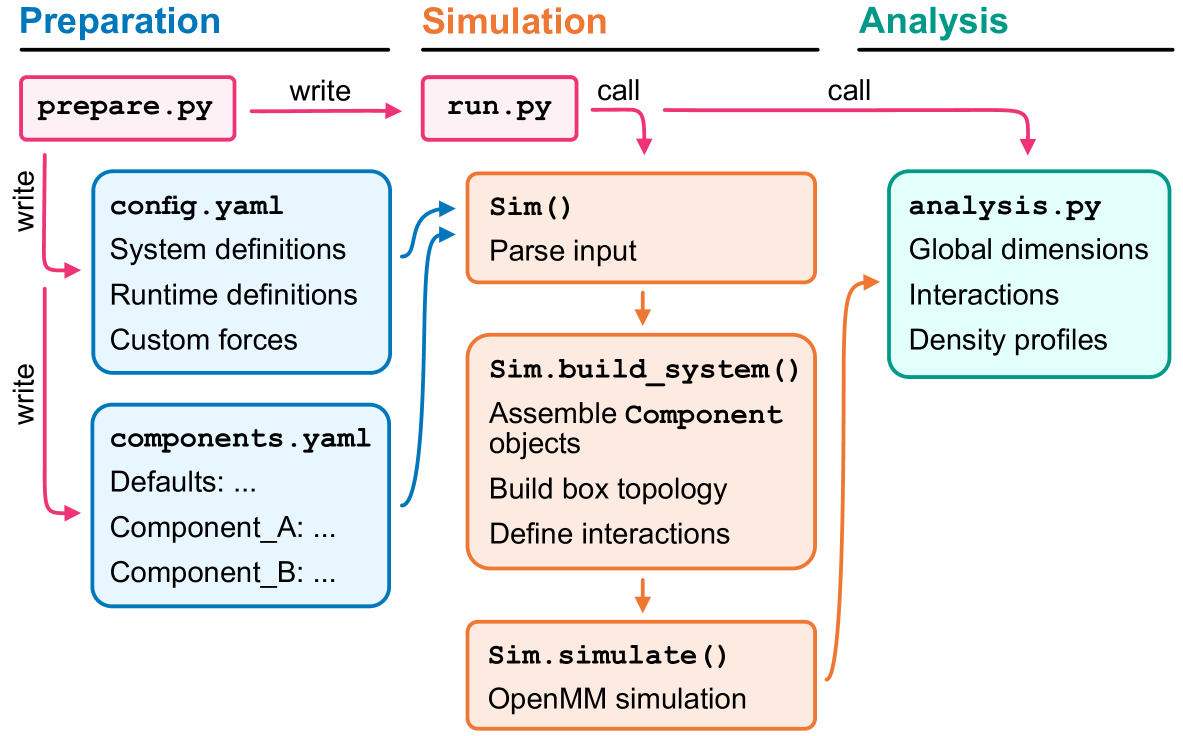
Figure 1: Architecture of the CALVADOS package. A wrapper script prepare.py generates the files config.yaml, components.yaml, and run.py for general definitions, molecule definitions, and running the simulation, respectively. run.py calls the main class Sim, which parses the input, handles setting up the system, and runs the OpenMM simulation. run.py can optionally be configured to call analysis scripts after the simulation is completed. Various trajectory post-processing and analysis routines for single-chain and multi-chain properties are included in the package.

2.2 User input

The user generally provides two input files: A system configuration file (default: config.yaml) and a component file (default: components.yaml). The system configuration file describes global parameters such as box dimensions, temperature, and pH. The component file defines the types and numbers of molecules together with other molecule-specific properties such as whether to account for charged moieties at the termini of polypeptide chains. A default section in the components.yaml configuration file can be used to define properties shared by all molecules. Molecule-specific definitions overwrite the default, allowing users to mix default settings with molecule-specific input. Additional input files such as custom residue definitions, folded domain definitions or custom restraints can be required depending on the specifications of the system and/or components.

The config.yaml and components.yaml input files can be written and edited manually. However, our package provides the Python wrapper prepare.py that conveniently generates both files together with a run.py script to start the simulation, and, optionally, batch job submission files to run the simulation on a server. The wrapper can be supplied with minimal definitions which are then combined with the default settings specified in the files calvados/data/default_config.yaml and calvados/data/default_component.yaml. Template job configuration files are also available (calvados/data/default_job.yaml) alongside batch submission script templates in jinja format (calvados/data/templates/). New job templates can be added to match the user’s server architecture. The cfg.py script manages the settings in the wrapper and writes the input files. The examples in Section 3 show a minimum wrapper (Section 3.1) and extensions thereof for different systems.

2.3 Sim class

The system setup is split into the Sim class of the sim.py module and the Component class of the components.py module. All general definitions and definitions pertaining to multiple components (e.g., intermolecular interactions) are dealt with by Sim, whereas all definitions at the level of a single molecule (e.g., bond connectivity, bead properties, geometry of the initial configuration, intramolecular restraints, etc.) are defined in the Component class.

The Sim class parses the input and sets up the simulation system. First, Sim.__init__() reads and processes the system configurations (config.yaml) and component (component.yaml) input files. Sim requires all relevant simulation parameters to be defined in these files.

Following input parsing, Sim.build_system() defines simulation box dimensions and periodic boundary conditions. For each different molecular component of the system, Sim then instantiates an object of the Component class (and subclasses thereof) in the components.py module, described in Section 2.4.

Molecules are then distributed in the box based on the keyword topol to generate a starting configuration (e.g., with molecules placed in the centre, randomly, in a slab, or on a grid), which is saved as a structure file in PDB format. Non-bonded interactions are defined and the general definitions, including information from each Component object, are packaged into an openmm.System object.

The simulate() method of Sim combines the input configuration, openmm.System object, a Langevin integrator (by default with time step $t=$10\text{\,}\mathrm{fs}$$ and friction coefficient $\gamma=$0.01\text{\,}\mathrm{ps}$^{-1}$), and a desired platform (CPU, OpenCL, or CUDA) to create an openmm.Simulation object. Finally, the simulation is run for a set number of steps or simulation time in hours.

2.4 Component class

In CALVADOS, a component refers to a specific molecule (e.g., the protein FUS) with attributes including sequence, number of molecules, charges, geometry, connectivity, and bond forces. Every different molecule has its own component object, whereas multiple copies of the exact same molecule belong to the same component object. For example, four FUS proteins share the same component object, whereas an additional single Ddx4 protein would have a separate component object.

Each type of biomolecule (protein, RNA, etc.) has its own subclass (Protein, RNA, etc.) which inherits from the Component class. The design principle behind this is that certain attributes between the different biomolecules are shared. For example, all the molecule types have a sequence, particle beads, a molecular weight, etc., whereas other properties are molecule-type specific.

A generic molecule in Component is processed as follows: Read in the sequence, calculate the number of residues and number of beads, determine molecular weights, determine particle bead sizes and $\lambda$ stickiness parameters for use in the AH potential, determine charges for use in the DH potential, and determine bond lengths. Finally, a geometry of the molecule is either read from the PDB file or built from scratch.

The subclasses, such as Protein or RNA, incorporate the definitions that are biomolecule specific by adding additional functions or overwriting default functions of Component, where needed. For example, the number of beads per residue and the connectivity of beads (define ‘what a bond is’) differ between the one-bead-per-residue protein model and two-bead-per-residue RNA model, as does the treatment of terminal residues in the RNA subclass. RNA also introduces additional angle and stacking potentials. In contrast, the Protein subclass has additional routines for restraining folded domains. This modularity allows for easy modification and addition of molecule definitions (see Section 4).

3 Tutorial examples

Below, we provide a number of examples to illustrate some of the types of applications that are made possible with the CALVADOS package. We note that our goal is generally not to motivate the science extensively or to discuss the results, but rather to illustrate how the package can be used and extended. We also stress the importance of reading the original literature for more details on the approximations involved, the ranges of applicability, and the extent to which different applications have been validated. All example scripts described in this section can be run from the examples folders on github.com/KULL-Centre/CALVADOS.

3.1 Single-chain IDR simulation

Using CALVADOS, we can simulate single IDRs and accurately predict their conformational properties providing as input the amino acid sequence, temperature, ionic strength, and pH of the buffer solution. In this example, we simulate the low-complexity domain (LCD) of the heterogeneous nuclear ribonucleoprotein (hnRNPA1^∗), hereafter A1-LCD^∗, with * indicating a sequence missing the hexa-peptide 259–264. hnRNPA1^∗, which is a splicing factor, consists of two RNA recognition motifs connected by a short linker, followed by the LCD: a 131-residue disordered C-terminal domain. This architecture is characteristic of many ribonucleoproteins which, in response to cell stress, together with RNA may form biomolecular condensates known as stress granules ⁵⁹. A1-LCD^∗ has been shown to be necessary and sufficient for the phase separation of hnRNPA1^∗ in vitro ^{59, 60}, and mutations within this region are implicated in neurodegenerative diseases, such as amyotrophic lateral sclerosis ⁶¹. The sequence features determining the compaction and phase properties of A1-LCD^∗ have been studied extensively ^{62, 63}.

To simulate a single copy of A1-LCD^∗, we initialise the Config class in the prepare.py script as follows:

config = Config(
    box=[50, 50, 50],  # nm
    topol=’center’,
    temp=293,          # K
    ionic=0.19,        # M
    pH=7.5,
    wfreq=7000,        # trajectory writing interval
                       # 1 step = 10 fs
    steps=1010*7000,   # 1010 frames
    )

With the options box and topol, we place the IDR in the centre of a cubic box with 50-nm side length and specify temp, ionic, and pH to set the same temperature, ionic strength, and pH as in the experimental SAXS measurements by Martin et al. ⁶⁰. By setting ionic equal to 0.190 M, we account for ionic strength contributions from salt (150 mM NaCl) as well as from the buffer (50 mM Tris at pH 7.5 contributes with $\approx 40$ mM to the ionic strength). We save frames to a trajectory DCD file every 7,000 MD steps, corresponding to $\Delta t=70$ ps. We run the simulation for 70,700 ps and discard the first 700 ps. These settings allow us to collect 1,000 weakly correlated conformations. In a previous study, we fine-tuned the saving frequency to sample consecutive configurations with a low extent of self-correlation irrespective of sequence length, $N$, and obtained $\Delta t\approx 3\times N^{2}\,$\mathrm{fs}$$ if $N>150$ and $\Delta t=70\,$\mathrm{ps}$$ otherwise ³⁶. With this empirical relationship, we found that the value of the autocorrelation function of the radius of gyration, for a time lag of one frame, plateaus to $\sim 0.5$ for $N>200$.

In the prepare.py script, we initialise default Components definitions as follows:

components = Components(
    molecule_type=’protein’,
    nmol=1,
    charge_termini=’both’,
    fresidues=f’{cwd}/input/residues_CALVADOS2.csv’,
    ffasta=f’{cwd}/input/idr.fasta’,
    )

molecule_type and nmol specify that we are simulating a single copy of a protein. With charge_termini=’both’, we add and subtract a unit charge to the N- and C-terminus, respectively, accounting for the extra positive charge and negative charge on the ammonium group at the N-terminus and the carboxylate at the C-terminus. N-, C-, and end-capped proteins can instead be simulated with the options charge_termini=’C’ (only adding a charge to C), ’N’ (only adding a charge to N), and ’end-capped’ (not adding any charge), respectively. We then specify the paths of the file containing the amino acid-specific parameters with fresidues, here parametrised using the CALVADOS 2 force field ⁴⁰, and the FASTA file with the IDR sequence with ffasta, where {cwd} should point to the current working directory.

The IDR of choice (A1SLCD in this case) is then added with

components.add(name=’A1SLCD’)

using the default settings defined above. All component defaults can be overwritten during the components.add() statement. This can be useful for multiple different components with, e.g., different numbers of molecules but otherwise equal definitions.

After running the simulations, the CALVADOS package also helps analyse the simulation trajectories, for example to calculate the internal-distance scaling exponent, $\nu$, the intra-chain residue-residue contacts, the end-to-end distance, $R_{ee}$, and the radius of gyration, $R_{g}$. We can perform these analyses right after the simulation run by adding the following lines in prepare.py:

subprocess.run(f’mkdir -p A1SLCD’, shell=True)
subprocess.run(f’mkdir -p data’, shell=True)
analyses = f"""
from calvados.analysis import save_conf_prop
save_conf_prop(
    path=’A1SLCD’, name=’A1SLCD’,
    residues_file=f’{cwd}/input/residues_CALVADOS2.csv’,
    output_prefix=’data’,
    start=10, is_idr=True, select=’all’
    )
"""
config.write(path, name=’config.yaml’, analyses=analyses)

First, we create directories to store the trajectory (A1SLCD) and the analysis files (data). Second, we write the script run.py appending to it two lines that, once the simulation has completed, import and call the function save_conf_prop(), which calculates per-frame $R_{ee}$ and $R_{g}$ values, the average contact map, and the average $\nu$ (Fig. 2A–C). We estimate $\nu$ from a nonlinear fit to $\sqrt{\langle R_{ij}^{2}\rangle}=R_{0}|i-j|^{\nu}$ of the root-mean-square residue-residue distances, $\sqrt{\langle R_{ij}^{2}\rangle}$, for separations along the linear sequence, $|i-j|$, larger than 5 (Fig. 2A). To obtain the contact map (Fig. 2B), we calculate residue-residue distances, $r_{ij}$, for $|i-j|>3$ and apply the switching function

$$c(r_{ij})=0.5-0.5\tanh{[(r_{ij}-r_{0})/w]}$$ (7)

where $r_{ij}$ is the intermolecular distance between two residues, $r_{0}=$1\text{\,}\mathrm{nm}$$, and $w=$0.3\text{\,}\mathrm{nm}$$. The CALVADOS package uses MDAnalysis ⁶⁴ and MDTraj ⁶⁵ to help in analysing the trajectories, and the user can use these and many other tools to analyse the trajectories in other ways.

A simulation performed with the settings detailed in this section takes 25 min on a single core of an AMD EPYC 9754 CPU and 3 min on an NVIDIA A40 GPU.

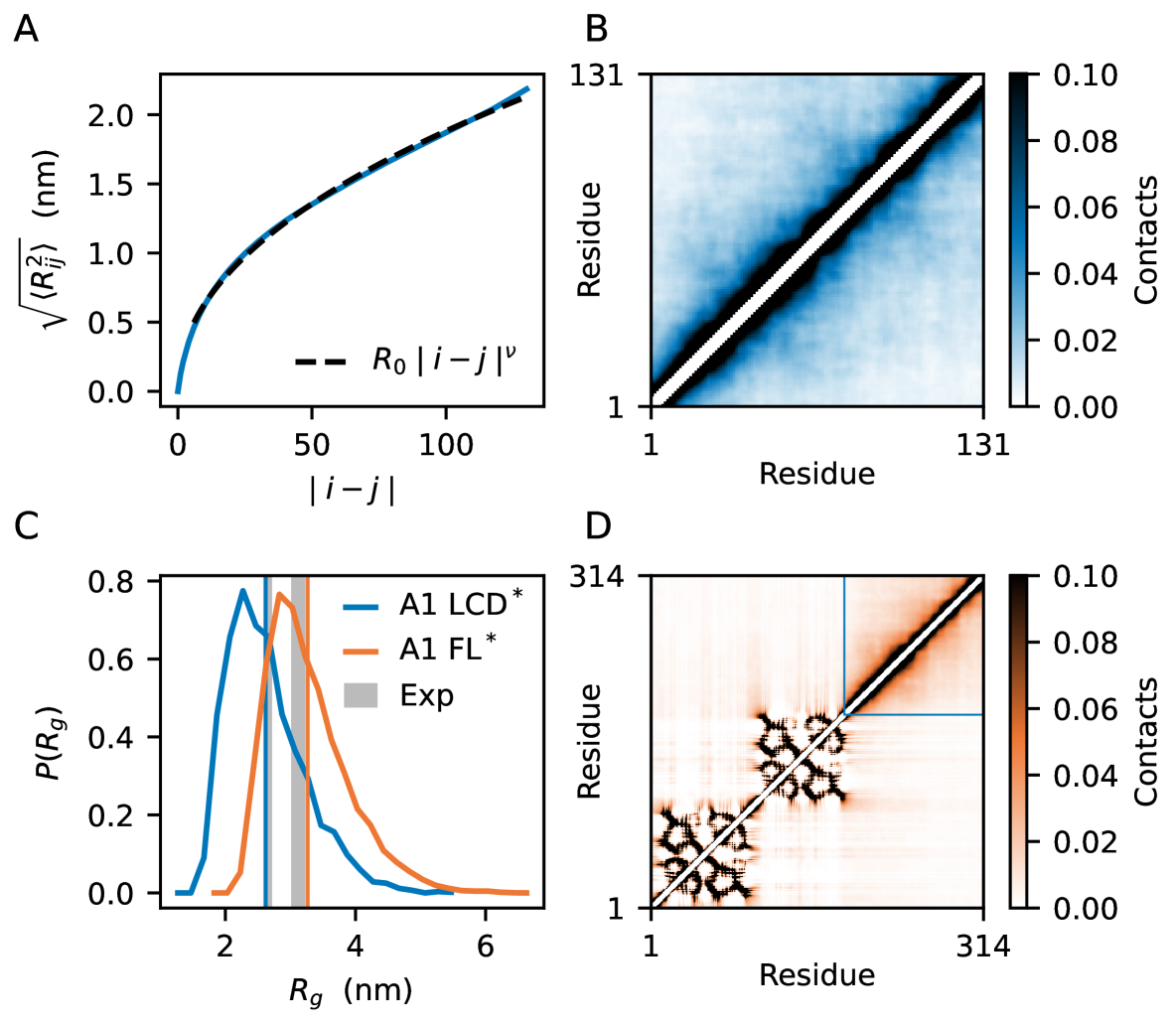
Figure 2: Single-chain simulations. (A) Root-mean-square residue-residue distances, $\sqrt{\langle R_{ij}^{2}\rangle}$, vs. separations along the linear sequence, $|i-j|$, calculated from single-chain simulations of A1-LCD^∗. Dashed line: nonlinear fit to $\sqrt{\langle R_{ij}^{2}\rangle}=R_{0}|i-j|^{\nu}$. (B) Intra-chain contact map of A1-LCD^∗. (C) Distributions of the radius of gyration, $R_{g}$, of A1-LCD^∗ and full-length hnRNPA1^∗. Vertical solid lines: ensemble-averaged simulated $R_{g}$. Vertical grey bars: confidence interval of the experimental $R_{g}$ values measured by Martin et al. ⁶⁰. (D) Intra-chain contact map of full-length hnRNPA1^∗. Blue box: LCD from residue 183 to residue 314. All simulation data shown in this figure are averaged over three independent replicas.

We performed three independent simulations of A1-LCD^∗ and estimated ensemble averages and the corresponding errors as the mean $\pm$ the standard deviation (SD) across the replicas. From the simulations we calculate an apparent scaling exponent of $\nu=0.473\pm 0.001$ (Fig. 2A), indicative of a compact conformational ensemble characteristic of a polymer chain in a poor solvent, where intra-chain interactions are more favourable than residue-solvent interactions. We note that, relative to the intrinsically disordered human proteome, A1-LCD^∗ is remarkably compact, with only 5% of IDRs estimated to have $\nu\leq 0.475$ ³⁶. The predicted $R_{g}$ of $2.62\pm 0.03$ nm is in good agreement with the experimental value reported by Martin et al. ⁶⁰ (Fig. 2C). To further illustrate the conformational ensemble, we calculate the intra-chain contact map and observe long-range interactions (Fig. 2B): Residue pairs separated by more than 20 positions along the sequence are in contact in up to 4% of the sampled conformations.

3.2 Single-chain MDP simulation

In this example, we perform a single-chain simulation of the MDP hnRNPA1^∗ and characterise its conformational ensemble. In addition to the input for simulating an IDR detailed in the previous section, for MDPs we provide a PDB file as the starting structure. This structure can be obtained from experiments or, for example, from AlphaFold predictions ⁶⁶. To restrain the folded domains and maintain their structure throughout the simulation, we use an elastic network model (ENM), whereas the IDRs of the MDP are modelled as flexible chains. To apply the ENM, we first identify the boundaries of each structured domain, for example by visual inspection of the three-dimensional protein structures. Each domain is then mapped to a sequence segment delimited by a start and an end residue. Only pairs of non-neighbouring residues within the same domain are restrained by the harmonic potential of the ENM. To provide the definitions of the domain boundaries, we create a domain file (domains.yaml by default) containing the following lines:

hnRNPA1S:
 - [11,89]
 - [105,179]

hnRNPA1S is the protein name, and [11,89] and [105,179] are two restrained domains: The first spanning residues 11–89 and the second residues 105–179 (1-based indexing, inclusive of the termini). For proteins that have long loops protruding from within a domain, one may exclude such loops in the domains by using nested lists:

SNAP_FUS:
 - [286, 368]
 - [423, 451]
 - [[537, 564], [586, 701]]

In this case, the protein SNAP_FUS has three restrained domains, of which the third contains a loop (residues 565–585) that we do not restrain.

We specify the MDP component as for simulations of single IDRs (Section 3.1), with the following modifications:

components = Components(
    restraint=True,                     # apply restraints
    fresidues=’{cwd}/input/residues_CALVADOS3.csv’,
    fdomains=’{cwd}/input/domains.yaml’,
    pdb_folder=’{cwd}/input’,
    use_com=True,                       # COM representation
    restraint_type=’harmonic’,
    k_harmonic=700,                     # force constant
    cutoff_restr=0.9,
    )

restraint=True indicates that the protein will be regarded as an MDP. For simulations of systems containing MDPs, we recommend using residues_CALVADOS3.csv, which was parametrised using experimental data for both IDRs and MDPs ⁵¹. We then use fdomains and pdb_folder to specify the path of the file containing the domain boundaries and the folder containing the PDB files. The name of the PDB file in pdb_folder should match the name of the component. With use_com=True, we set the centre-of-mass representation for the restrained folded domains. We define the ENM with restraint_type=’harmonic’, set the force constant using k_harmonic (default: $700\text{\,}\mathrm{kJ}\text{\,}{\mathrm{mol}}^{-1}$), and apply restraints to residue pairs separated by up to cutoff_restr (default: $0.9\text{\,}\mathrm{nm}$). As in the previous example, we performed three independent simulations and used the SD over the ensemble averages across the replicas as an estimate of the sampling error. To calculate per-frame $R_{ee}$ and $R_{g}$ values, and the average contact map, we included the same lines in prepare.py as for the example in Section 3.1, setting is_idr=False to skip the calculation of $\nu$.

The $R_{g}$ distribution of full-length hnRNPA1^∗ is shifted toward larger values compared to that of its C-terminal LCD (Fig. 2C) and has a mean of $R_{g}=3.27\pm$0.01\text{\,}\mathrm{nm}$$, in good agreement with the experimental measurement ($3.12\pm$0.08\text{\,}\mathrm{nm}$$) ^{60, 17}. The intra-chain contact map highlights long-range interactions between the folded RRMs and the LCD (Fig. 2D), consistent with previous observations ⁶⁰. A simulation of full-length hnRNPA1^∗ performed with the settings detailed in this section has a speed of 250 ns/day on a single core (750 ns/day on 4 cores and 1000 ns/day on 8 cores) of an AMD EPYC 7552 CPU and $36.4\text{\,}\mathrm{\SIUnitSymbolMicro s}$/day on an NVIDIA A40 GPU.

3.3 Simulation of two (or more) different IDPs

CALVADOS can be used to simulate systems of several IDPs to predict the strength and mode of IDP-IDP interactions, as well as the influence of interaction partners on the conformational properties of individual chains. In the simplest case, we can simulate two chains with identical sequences and characterise the self-interaction of the IDP. Here, we simulate a heterogeneous two-chain system consisting of one copy of $\alpha$-synuclein ($\alpha$-Syn) and one copy of Tau35, a fragment that spans residues 187–441 of full-length human tau (ht2N4R). The steps outlined in the following can also be used to simulate and analyse more complex mixtures with several copies of many different IDPs. Two-chain simulations of $\alpha$-Syn (sequence length 140 residues) and Tau35 (sequence length 255 residues) run with a speed of $30\text{\,}\mathrm{\SIUnitSymbolMicro s}$/day on an NVIDIA V100-16GB GPU with the settings described below.

In the prepare.py script, we instantiate the Config class as illustrated above for single-chain systems, for example with a box size and solution conditions to match experimental data. In this example, we used box=[40, 40, 40], wfreq=10000, steps=5e8, temp=288, ionic=0.12, and pH=7.2. The system contains two components, one for each type of protein. We specify the component defaults as for the single-IDR example (Section 3.1), and then add each component to our system with components.add():

components = Components(
    ... # defaults as for the single-chain IDR example
    )
components.add(name=’aSyn’)     # add single copy of aSyn
components.add(name=’Tau35’)    # add single copy of Tau35

To characterise the interaction between the two IDPs, we used the two-chain simulation trajectory to calculate the radial distribution function, $g(r)$, and the residue-residue contacts between the proteins. $g(r)$ is a function of the inter-chain separation, $r$, which is commonly computed as the distance between the COMs of the two chains. We can add the following lines in prepare.py to run the analysis functions calc_contact_map() and calc_com_traj() immediately after the simulation is completed to generate a trajectory file in which each IDP is represented by its COM, and to calculate the inter-chain contact map:

subprocess.run(f’mkdir -p aSyn_Tau35’,shell=True)
subprocess.run(f’mkdir -p aSyn_Tau35/data’,shell=True)
analyses = f"""
from calvados.analysis import calc_com_traj, calc_contact_map
# dictionary of chain indices
# 0-based indexing
chainid_dict = dict(’aSyn’ = 0, ’Tau35’ = 1)
calc_com_traj(
    path=’aSyn_Tau35’, sysname=’aSyn_Tau35’, output_path=’data’,
    residues_file=’{cwd}/input/residues_CALVADOS2.csv’,
    chainid_dict=chainid_dict, start=10
    )
calc_contact_map(
    path=’aSyn_Tau35’, sysname=’aSyn_Tau35’,
    output_path=’data’, chainid_dict=chainid_dict
    )
"""
config.write(path,name=’config.yaml’,analyses=analyses)

Using the COM-based trajectory, we compute COM–COM separations for each simulation frame (Fig. 3A) and use these to calculate $g(r)$ (Fig. 3B). The second virial coefficient, $B_{2}$, can be calculated from $g(r)$ through the following integral:

$$B_{2}=-2\pi\int_{0}^{R_{c}}[g(r)-1]r^{2}dr,$$ (8)

where $r$ is the COM–COM separation, and the upper limit of integration, $R_{c}$, is set to half the edge length of the cubic simulation box or less. For large values of $r$, $g(r)$ should approach one, as the interactions between the chains vanish. However, for systems of finite size, $g(r)$ can deviate significantly from one also at large values of $r$ (Fig. 3B). In our example, the attractive interaction between the two chains leads to a local accumulation at short separations, which in turn causes a depletion at larger separations, relative to the bulk concentration in the simulation box. Different methods have been proposed to correct for this finite-size effect prior to calculating $B_{2}$ ^{67, 68}. We here used the correction proposed by Ganguly and van der Vegt ⁶⁷ and obtained $B_{2}=-2\pm 1$ L mol kg^-2.

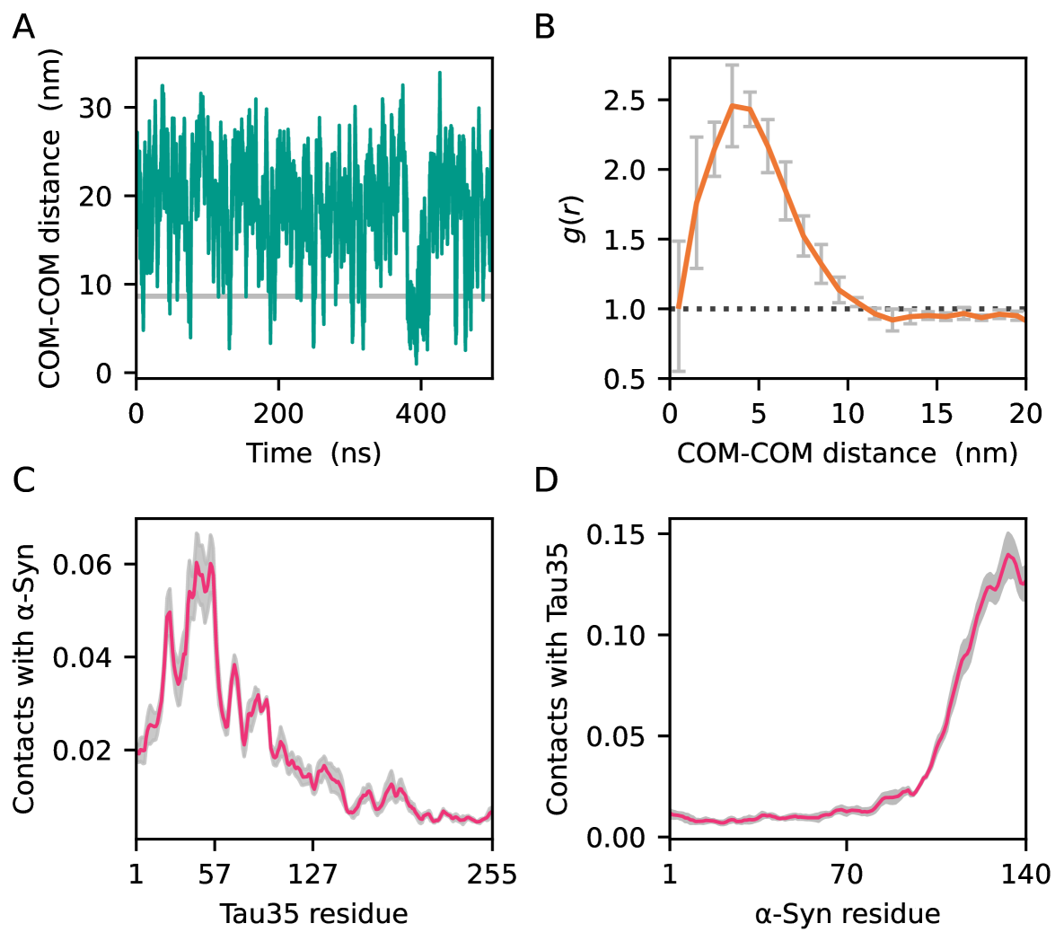
Figure 3: Simulation of two different IDPs. (A) Time series of aSyn-Tau35 COM–COM separation shown for $500\text{\,}\mathrm{ns}$ (5,000 simulation frames). Grey horizontal line: sum of the average radii of gyration of $\alpha$-Syn and Tau35. (B) Radial distribution function, $g(r)$, as a function of the aSyn-Tau35 COM–COM separation, $r$. $g(r)$ is averaged across three independent simulation trajectories, and error bars show the SD across the three runs. Dotted black line: $g(r)=1$. (C) Total number of time-averaged contacts formed between residues in Tau35 and any residue in $\alpha$-Syn. (D) Total number of time-averaged contacts formed between residues in $\alpha$-Syn and any residue in Tau35. The total contacts are averaged across three independent simulations, and grey shaded areas show the SD across the three replicas.

While $B_{2}$ indicates the strength of the inter-chain interaction, and whether this is net attractive ($B_{2}<0$) or net repulsive ($B_{2}>0$), our simulations also provide information on which residues are involved in the formation of the transient dimer. By summing the two-dimensional contact map along each axis, we calculate the time-averaged contacts formed by each residue of one chain with all the residues of the other (Fig. 3C and D). Our simulations reveal that the residues engaging in transient inter-chain interactions are predominantly in the N-terminal region of Tau35 and in the C-terminal region of $\alpha$-Syn. This is in accordance with experimental NMR chemical shift perturbations, which show that $\alpha$-Syn and full-length human tau interact via the negatively charged C-terminal domain of $\alpha$-Syn and the positively charged P2 region of full-length tau (residues 12–57 in Tau35) ⁶⁹.

3.4 Single-component slab simulation

In this example, we show how to simulate and analyse a system of multiple IDR chains that phase separate and form a protein-rich condensed (dense) phase in equilibrium with a dilute phase. To reduce the impact of finite-size effects when simulating the coexistence of these two phases, we insert the proteins into an elongated box with equal side lengths along the $x$- and $y$-axes ($L_{x}=L_{y}$), and a length along the $z$-axis ten times larger ($L_{z}=10\times L_{x}$). With such a simulation cell, proteins may spontaneously phase separate into a single slab spanning the periodic images along the $x$- and $y$-axes ⁷⁰, ²⁷. This setup minimises the interface area and allows us to approximate a bulk dense phase with only one or a few hundred copies of a protein. The long $L_{z}$ is needed to sample the dilute phase which has a concentration much smaller than the dense phase.

The key setting for a slab simulation are shown in the following snippet:

config = Config(
    ... # define temp, ionic, pH
    box=[15, 15, 150],    # nm
    topol=’slab’,         # place chains in a slab
    slab_width=20,        # of width 20 nm
    slab_eq=True,         # apply linear potential
    steps_eq=5000000,     # for this many steps
    wfreq=50000,
    steps=5400*50000      # 2.7 s
    )

With topol=’slab’, we speed up the equilibration of the two-phase system by first inserting the chains between $z=-10$ nm and $z=10$ nm (slab_width=20), with $x$- and $y$-coordinates on a regular grid. We then apply a linear external potential $u_{\text{ext}}(z)=k\,|z-L_{z}/2|$, with $k_{\text{eq}}=0.02$ kJ mol^-1 nm^-1, to focus the chains towards the midplane of the box ($z=0$). The potential is applied for the first $50\text{\,}\mathrm{ns}$ (steps_eq=5000000), during which the trajectory is saved to a file with prefix ‘equilibration_’. Subsequently, we remove the restraint and simulate the systems for additional $2.7\text{\,}\mathrm{\SIUnitSymbolMicro s}$, of which the initial $0.2\text{\,}\mathrm{\SIUnitSymbolMicro s}$ are discarded for equilibration. Simulations of A1-LCD, performed with the settings detailed in this section, have a speed of $5.8\text{\,}\mathrm{\SIUnitSymbolMicro s}$/day on an NVIDIA A40 GPU.

In the package, we implemented the class SlabAnalysis which features basic routines to analyse slab simulations, as shown in the snippet below.

from calvados.analysis import SlabAnalysis
slab = SlabAnalysis(
            name=’A1LCD’, input_path=’A1LCD’,
            output_path=’data’, ref_name=’A1LCD’,
            verbose=True
            )
slab.center(start=400, center_target=’all’)
slab.calc_profiles()
slab.calc_concentrations(pden=2, pdil=8)

First, we run center() to calculate instantaneous concentration profiles in the production run (start=400) and use these to shift the positions of all the beads, so as to align the slab in the middle of the box in each frame. With the resulting centred trajectory, we run calc_profiles() to recalculate the instantaneous concentration profiles and their average over time (Fig. 4A and B). When the simulation converges, the profile is approximately symmetric around $z=0$. To obtain the concentrations in the coexisting phases, we run calc_concentrations(). This function finds the position of the dividing surface, $z_{\text{DS}}$, and the thickness of the interface, $2\cdot d$, by fitting the half profiles for $z<0$ and $z>0$ to the sigmoidal function

$$c(z)=\frac{\widehat{c_{\text{den}}}+\widehat{c_{\text{dil}}}}{2}+\frac{\widehat{c_{\text{dil}}}-\widehat{c_{\text{den}}}}{2}\tanh{\left(\frac{|z|-z_{\text{DS}}}{d}\right)},$$ (9)

where $\widehat{c_{\text{den}}}$ and $\widehat{c_{\text{dil}}}$ are estimates of the average concentrations of the dense and dilute phases, respectively. Using the best-fit parameters, calc_concentrations() then calculates the time series of $c_{\text{den}}$ and $c_{\text{dil}}$ from the mean concentrations in $|z|<z_{\text{DS}}-p_{\text{den}}\cdot d$ and $|z|>z_{\text{DS}}+p_{\text{dil}}\cdot d$, where $p_{\text{den}}$ and $p_{\text{dil}}$ can be defined by the user and are set by default to 2 and 8, respectively. The output generated by these functions includes the slab-centred trajectory, the time-averaged concentration profile (Fig. 4A), the time series of the concentration profile (Fig. 4B), the time series of $c_{\text{den}}$ and $c_{\text{dil}}$, and a table summarizing the settings and results of these analyses.

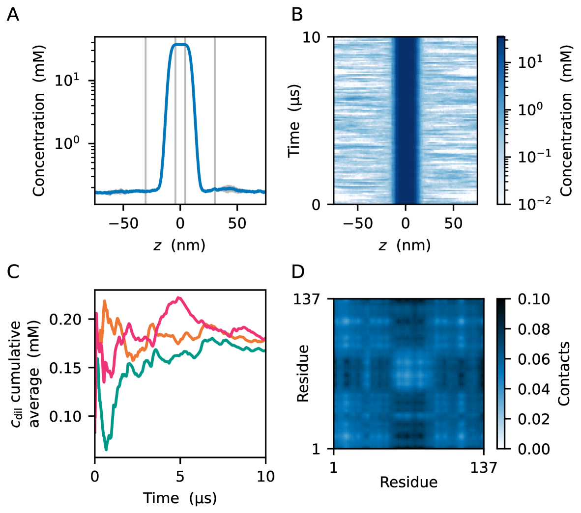
Figure 4: Single-component slab simulation. (A) Concentration profile of hnRNPA1 LCD along the $z$-axis of the simulation cell. The profile is averaged over three simulation replicas with the grey shaded areas showing the SD. Grey vertical lines: boundaries defining the regions within which we calculate the concentration in the dense phase, $c_{\text{den}}$, and in the dilute phase, $c_{\text{dil}}$. (B) Instantaneous concentration profiles as a function of simulation time. (C) Cumulative averages of $c_{\text{dil}}$ from three independent simulation replicas. (D) Contact map between the chain closest to the mid-plane of the protein-dense slab and the surrounding chains.

The saturation concentration, $c_{\text{sat}}$, of the dilute phase at equilibrium with a biomolecular condensate is particularly sensitive to changes in amino acid sequence and solution conditions ⁷¹, and is often used to quantify the propensity of a biomolecule to phase separate. Therefore, $c_{\text{sat}}$ is a key parameter to benchmark simulations against experiments. In this example, we simulated the 137-residue-long LCD of hnRNPA1 (A1-LCD), without the nuclear localization signal ⁶², ⁶³, in three independent simulation replicas, setting temp=293 and ionic=0.15. In good agreement with the experimental $c_{\text{sat}}$ value of $102.2\pm 0.4\,$\mathrm{\SIUnitSymbolMicro M}$$ ^{62, 63}, we estimate $c_{\text{dil}}=176\pm 6\,$\mathrm{\SIUnitSymbolMicro M}$$ as the mean $\pm$ SD across the three replicas. To ensure the convergence of the mean $c_{\text{dil}}$, a simulation time of around $7\text{\,}\mathrm{\SIUnitSymbolMicro s}$ is required for this system, as shown by the cumulative averages of $c_{\text{dil}}$ for the three replicas (Fig. 4C).

In addition to estimating thermodynamic properties, such as $c_{\text{sat}}$ and transfer free energy, $\Delta G_{\text{trans}}=RT\ln{(c_{\text{dil}}/c_{\text{den}})}$, slab simulations provide molecular-level insight into intermolecular interactions in the coexisting phases. Using the function calc_com_traj() introduced in Section 3.4, we obtain the trajectory of the centres of mass of all the chains in the system. The function calc_contact_map() uses this file to find, in each frame, the chain that is closest to the midplane of the slab, and calculates the residue-residue distances, $r_{ij}$, between this chain and all surrounding chains. We convert these distances into contacts using the switching function in Eq. 7. The contact map for A1-LCD in the condensate (Fig. 4D) highlights the strong attractive interactions between the positively charged N-terminal and C-terminal regions and the negatively charged and aromatic-rich region between residues 50 and 90.

# calculate homotypic contact map
from calvados.analysis import calc_com_traj, calc_contact_map
# dictionary of chain indices
# 0-based indexing, inclusive
chainid_dict = dict(A1LCD = (0, 99))
calc_com_traj(
    path=f’{cwd}/A1LCD’, sysname=’A1LCD’,
    output_path=f’{cwd}/data’,
    residues_file=f’{cwd}/input/residues_CALVADOS2.csv’,
    chainid_dict=chainid_dict
    )
calc_contact_map(
    path=f’{cwd}/A1LCD’, sysname=’A1LCD’,
    output_path=f’{cwd}/data’,
    chainid_dict=chainid_dict,
    is_slab=True
    )

3.5 Slab simulation of mixed systems

Many IDRs undergo phase separation with nucleic acids; in this section, we simulate an example of such a mixed system, consisting of the RGG3 domain of Fused in Sarcoma (FUS-RGG3) and a 40-base polyuracil strand (polyU40). Although FUS-RGG3, which is positively charged, does not easily phase separate alone, the addition of moderate amounts of RNA induces phase separation ⁷². Since the two-bead-per-residue RNA model is sequence independent, a specific strand is defined solely by its length; in this case, by specifying 40 consecutive r characters in the FASTA file (idr.fasta). In the script prepare.py, we set up a system containing 200 chains of FUS-RGG3 and 60 chains of polyU40 and describe these using the CALVADOS 2 model for proteins ⁴⁰ and the CALVADOS-RNA model ⁵⁴ via residues_C2RNA.csv. The instantiation of Components and the lines for adding the chains are as follows:

components = Components(
    fresidues=f’{cwd}/input/residues_C2RNA.csv’,
    ffasta=f’{cwd}/input/idr.fasta’,
    rna_kb1=1400.0, rna_kb2=2200.0,
    rna_ka=4.20, rna_pa=3.14,
    rna_nb_sigma=0.4, rna_nb_scale=15,
    rna_nb_cutoff=2.0
    )
components.add(
    name=’FUS-RGG3’, molecule_type=’protein’,
    nmol=100,  charge_termini=’both’
    )
components.add(
    name=’polyU40’, molecule_type=’rna’, nmol=60
    )

The parameters set through the Config object are the same as for the single-component system of Section 3.1, except for box=[15, 15, 80], wfreq=100000, steps=100000000, and the solution conditions, which we match to those of Kaur et al. ⁷², namely temp=293.15, ionic=0.15, and pH=7.5. The performance of this simulation is $7.5\text{\,}\mathrm{\SIUnitSymbolMicro s}$/day using an NVIDIA GeForce RTX 3090 GPU and a single thread (AMD Ryzen Threadripper 3960X 24-Core Processor).

The simulation trajectory can be analysed to determine the distributions of proteins and RNA chains in the dilute and protein-dense phases. As in the previous example, center() removes the overall motion of the condensate by translating its centre to the midplane of the elongated box (Fig. 5A). After discarding the initial 250 steps for equilibration, calc_profiles() reads the translated trajectory and computes the concentration profiles of FUS-RGG3 and polyU40 (Fig. 5B). Finally, calc_concentrations() identifies the dilute and dense phase regions and computes their mean concentration for each frame (Figs. 5C and D). From the density profiles and concentration time series (Figs. 5B and C), we estimate the concentration ratio of FUS-RGG3 to RNA within the condensate to be approximately 4:1. These analyses can be executed by adding the following lines to prepare.py:

from calvados.analysis import SlabAnalysis
slab_analysis = SlabAnalysis(
    name=’mixed_system’,
    input_path=f’{cwd}/mixed_system’,
    output_path=f’{cwd}/data’,
    input_pdb=’top.pdb’, input_dcd=None,
    centered_dcd=’traj.dcd’,
    # use proteins as reference for centering
    ref_chains=(0, 199),  # 0-based indexing, inclusive
    ref_name=’FUS-RGG3’,
    client_chain_list=[(200, 259)],
    client_names=[’polyU40’],
    verbose=False
    )
slab_analysis.center(
    start=250,
    center_target=’ref’
    )
slab_analysis.calc_profiles()
slab_analysis.calc_concentrations()

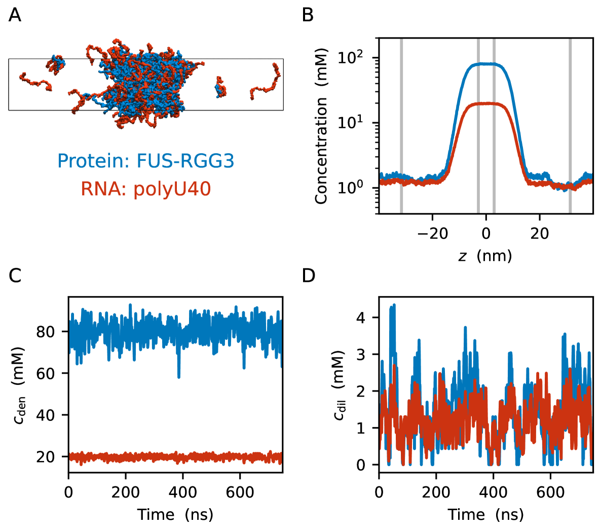
Figure 5: Slab simulation of protein and RNA. (A) A representative snapshot showing FUS-RGG3 in blue and polyU40 in red. (B) Concentration profile of FUS-RGG3 and polyU40 along the $z$-axis. Grey vertical lines: boundaries of dilute and dense phases. Time series of the concentration of FUS-RGG3 and polyU40 in the (C) dense and (D) dilute phases.

3.6 Simulations with crowders

The environment of an IDP can have a significant effect on its conformational dynamics. To study the effects of macromolecular crowding in the CALVADOS model, we have implemented a model for the synthetic crowding agent polyethylene glycol (PEG) ⁵⁵. In our PEG model each bead represents a single residue, and PEG polymers of different molecular weights are represented by sequences of varying lengths, with the letter J denoting the PEG monomer in the FASTA file. To illustrate what effects can be modelled, we here simulate two different systems, (i) a single chain of an IDR (ACTR) with increasing concentrations of PEG400, and (ii) a slab of A1-LCD with increasing concentrations of PEG8000. In the first case, our model is applied to study how crowding affects the global dimensions of an IDP (Fig. 6A). In the second case, we show how a PEG-titration can be used to determine the phase separation propensity of an IDP in the absence of PEG (Fig. 6B).

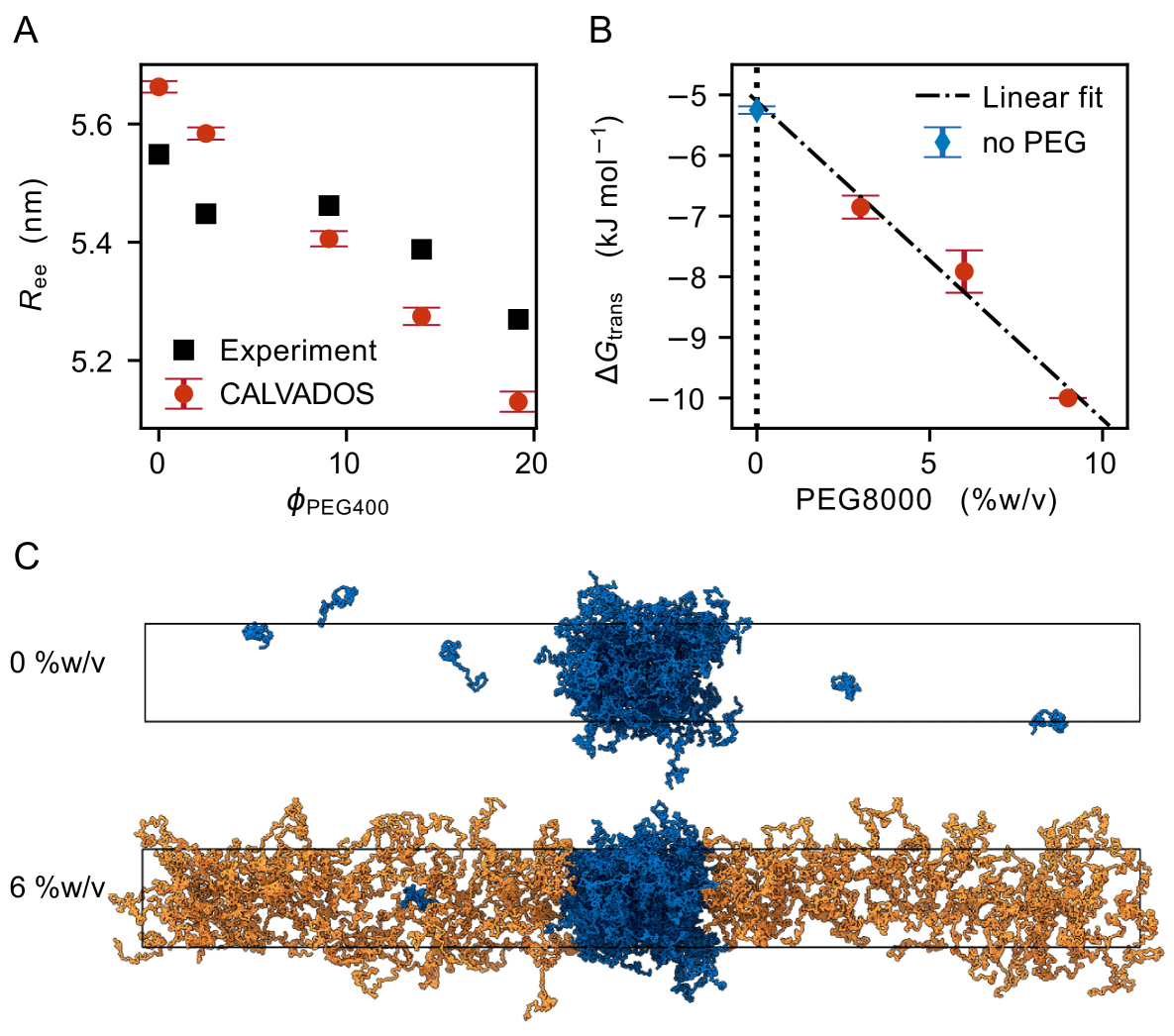
Figure 6: Simulations of IDPs in the presence of PEG. (A) End-to-end distances ($R_{\text{ee}}$) of a single chain of ACTR at increasing concentrations of PEG400. The figure shows previously generated simulation data ⁵⁵ and a comparison to experimental data ⁷³. (B) Phase separation propensity ($\Delta G_{\text{trans}}$) of A1-LCD with PEG8000 (red dots). A linear fit to the data generated at three different concentrations of PEG is used to extrapolate the phase separation propensity in the absence of PEG ($y$-intercept = $-5.1\pm 0.6\text{kJ~mol}^{-1}$). Blue diamond: $\Delta G_{\text{trans}}$ from a simulation of A1-LCD in the absence of PEG ($-5.25\pm 0.06\text{kJ~mol}^{-1}$). (C) Representative snapshots of slab simulations of A1-LCD without PEG8000 (100:0) and with 6 %w/v PEG8000 (100:152).

Before starting the simulations, we first calculate the number of PEG chains, $N_{\text{PEG}}$, as

$$N_{\text{PEG}}(\%\text{w/v PEG})=\frac{10\times\text{\%w/v}}{\text{MW}_{\text{PEG}}}\times V_{\text{box}}\times N_{A},$$ (10)

where $\%w/v$ is the PEG mass concentration in g/100 mL, $\text{MW}_{\text{PEG}}$ is the molecular weight of PEG, $V_{\text{box}}$ is the volume of the simulation box, and $N_{\text{A}}$ is Avogadro’s number. For direct comparison with experiments, we convert $\%w/v$ into the volume fraction, $\phi_{\text{PEG}}$, using $\phi_{\text{PEG}}=(10\times\text{\%w/v})/\rho_{\text{PEG,bulk}}$, where $\rho_{\text{PEG,bulk}}=1,120$ g/L ⁷³, ⁵⁵.

To set up the simulations, the configuration settings are defined as for a standard slab simulation except for the PEG-model specific parameter fixed_lambda, which fixes the AH stickiness parameter $\lambda$ to 0.2 for PEG–PEG and protein–PEG interactions ⁵⁵.

config = Config(
    ... # general definitions
    topol=’grid’,
    fixed_lambda=0.2
    )

Additionally, the bead size $\sigma$ and the MW of a PEG monomer are defined in residues_C2PEG.csv and read as usual:

components = Components(
    ...
    fresidues=f’{cwd}/input/residues_C2PEG.csv’
)

To simulate ACTR with PEG, we use the experimental conditions ⁷³, namely temp=295.15, ionic=0.11 and pH=7.5. We add a single chain of ACTR (nmol=1) and $N_{\text{PEG}}$ molecules of PEG400 (nmol=N_PEG) as follows:

components.add(name=’ACTR’, molecule_type=’protein’, nmol=1)
components.add(
    name=’PEG400’, molecule_type=’crowder’,
    nmol=N_PEG, charge_termini=False
    )

The conformational properties of the IDR are analysed as described in Section 3.1, now selecting only the protein chain in save_conf_prop(), by specifying select=’not resname PEG’. The end-to-end distance of ACTR, $R_{\text{ee}}$, as a function of $\phi_{\text{PEG400}}$ shows a decrease of $R_{\text{ee}}$ induced by the crowder (Fig. 6A).

With minor changes to the input shown in Section 3.4, we can perform slab simulations with PEG to mimic a PEG titration experiment and determine, by extrapolation, the phase separation propensity ($\Delta G_{\text{trans}}$) of a protein that is weakly prone to phase separate. Instead, in this example, we simulate the same IDR as in Section 3.4 and compare the value extrapolated from the PEG titration to $\Delta G_{\text{trans}}$ calculated from slab simulations for the IDR without any PEG.

As for the single-component system, the topology keyword is set to slab and we specify slab_width=20 to insert the proteins between $z=-10$ nm and $z=10$ nm. In addition, slab_outer=25 places the crowder molecules around the slab at $|z|>25$ nm.

config = Config(
    ... # general definitions as above
    box=[15, 15, 150],  # nm
    topol=’slab’,       # place proteins in a slab
    slab_width=20,      # of width 20 nm
    slab_outer=25,      # and the crowder outside
    fixed_lambda=0.2,
)
...
components.add(name=’A1LCD’, molecule_type=’protein’, nmol=100)
components.add(
    name=f’PEG8000’, molecule_type=’crowder’,
    nmol=N_PEG, charge_termini=False
    )

The performance of these protein–crowder simulations ranges from $4.75\text{\,}\mathrm{\SIUnitSymbolMicro s}$/day without PEG to $3.8\text{\,}\mathrm{\SIUnitSymbolMicro s}$/day with 3 %w/v PEG8000 to $2.1\text{\,}\mathrm{\SIUnitSymbolMicro s}$/day at 9 %w/v PEG8000 on a NVIDIA Tesla V100. The density profiles and concentrations of protein and PEG in the dense and dilute phases are calculated as for the mixed protein–RNA simulation in Section 3.5.

from calvados.analysis import SlabAnalysis
slab = SlabAnalysis(
    name=’A1LCD_PEG8000’,
    input_path=f’{cwd}/A1LCD_PEG8000’,
    output_path=f’{cwd}/data’,
    ref_name=’A1’, ref_chains=(0, 99),
    client_names=[’PEG8000’],
    client_chain_list=[(100, 99 + N_PEG)]
    )
slab.center(
    center_target=’ref’ # for centering only on A1LCD
    )
slab.calc_profiles()
slab.calc_concentrations()

To determine the phase-separation propensity of the protein in the absence of PEG, we perform a linear fit and extrapolate $\Delta G_{\text{trans}}$ without PEG as the $y$-intercept. For the case of A1-LCD, we find that this approach reproduces the value from a simulation without PEG (Fig. 6B).

3.7 Custom restraints

The CALVADOS package allows users to define custom restraints between any pairs of residues in the system. In prepare.py, custom restraints are enabled via

config = Config(
    ... # general definitions
    custom_restraints=True,
    custom_restraint_type=’harmonic’,
    fcustom_restraints=f’{cwd}/input/cres.txt’,
)

where the text file cres.txt contains the list of custom restraints. As an example, we restrain the two RRM domains in full-length hnRNPA1^{∗ 60} to move as a single domain ⁷⁴ and analyse the inter-domain fluctuations via the SD of the residue pair distances across the simulation. The cres.txt file reads

hnRNPA1S 1 72 | hnRNPA1S 1 157 | 0.559 700.0
hnRNPA1S 1 73 | hnRNPA1S 1 161 | 1.072 700.0
hnRNPA1S 1 75 | hnRNPA1S 1 155 | 0.765 700.0
...

with the syntax

component1 copy1 residue1 | component2 copy2 residue2 | r0 k

defining a harmonic bond with parameters as in Eq. 1. In this example, we only have one copy of a single component and restrain residues 72 with 157, 73 with 161, etc. using the corresponding COM-COM separations in the input structure (in nm) as the equilibrium distances. These restraints strongly affect how the RRMs move together in the simulation (Fig. 7). Whereas the unrestrained RRMs tumble more independently than suggested before ⁶⁰, ⁷⁴ and by the AlphaFold2 predicted aligned error (PAE) matrix (Fig. 7B and C), the custom restraints cause the RRMs to move together (Fig. 7D).

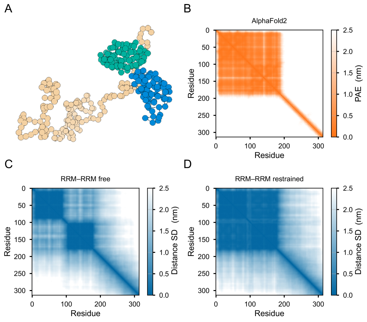
Figure 7: Full-length hnRNPA1^∗ simulations without and with custom restraints between key residues at the RRM–RRM interface. (A) Snapshot of coarse-grained full-length hnRNPA1^∗ with the RRMs coloured in green and blue. (B) AlphaFold2 predicted aligned error (PAE). SD of residue–residue distances (C) without or (D) with RRM-RRM restraints.

4 Modification and extension of the package

The modular architecture of the software allows for modifications and extensions, and contributions from the community are welcome. The CALVADOS code is hosted on GitHub (github.com/KULL-Centre/CALVADOS) and is made available with a GNU General Public License v3.0. We show three examples of simple CALVADOS extensions: Cyclic peptides, star-shaped polymers and residues with post-translational modifications (Fig. 8).

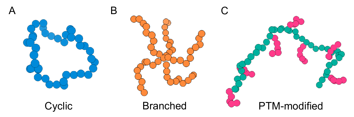
Figure 8: Example of how CALVADOS may be extended. Each of the examples is a subclass of Protein with minor modifications to bond definitions (A) cyclic, (B) branched, and (C) PTM-modified.

As the first example, we derive a new component class Cyclic that inherits from the Protein component class. Here, we change the criteria for the bond definitions by modifying bond_check() from

condition = (j == i + 1)

to

condition0 = (j == i + 1)
condition1 = (j == self.nbeads - 1) and (i == 0)
condition = condition0 or condition1

In this way, a bond is defined between the first and last residue (self.nbeads - 1) as well as between neighbouring residues in the sequence, creating a cyclic peptide (Fig. 8A).

As the second example, we create branched star-shaped polymers, again by modifying the bond_check() method. We define a central bead, adding bonds to that bead and removing bonds at the end of the ‘arms’ (Fig. 8B).

if self.n_ends in [0, 1, 2]:
    return super().bond_check(i, j)
else:
    if (self.nbeads - 1) % self.n_ends == 0:
        branch_length = int((self.nbeads - 1) / self.n_ends)
    else:
        branch_length = int((self.nbeads - 1) / self.n_ends) + 1
    condition0 = (j == i + 1) and ((j - 1) % branch_length != 0)
    condition1 = (i == 0) and ((j - 1) % branch_length == 0)
    condition = condition0 or condition1
    return condition

The number of ‘arms’ of the branched ‘seastar’ polymer can be chosen as an attribute n_ends in the component definition in prepare.py.

components.add(
    name=’branched_polymer’,
    molecule_type=’seastar’, n_ends=5
    )

As a final example, we introduce post-translational modifications (PTMs). There are at least two ways of incorporating PTMs into CALVADOS: As a first option, we modify or add amino-acid residue definitions to account for changes in charge or stickiness (e.g., caused by phosphorylation) without explicitly changing the number of beads. For CALVADOS, we parametrised phosphorylated serine (pSer) and threonine (pThr) beads with increased size and molecular weight, decreased stickiness, and partial charges computed based on solution pH and experimental p$K_{a}$ ^{75, 76}. We determined stickiness parameters for pSer and pThr using a top-down approach, targeting experiments on global dimensions for a set of phosphorylated and unphosphorylated IDRs ⁷⁶. This procedure resulted in a model with $\lambda_{\text{pSer}}\approx 0.09$ and $\lambda_{\text{pThr}}\approx 0.00$ ⁷⁶, though we note that it may also be possible to generate parameters using bottom-up procedures ⁷⁷, ⁷⁸.

Here, we show how to simulate the 10-fold phosphorylated IDR Ash1 with our phosphorylation model ⁷⁶. The first step is to prepare the sequence in FASTA format with the single letter codes B and O for pSer and pThr, respectively.

>10pAsh1
SASSBPBPSOPTKSGKMRSRSSBPVRPKAYOPBPRBPNYHR
FALDBPPQBPRRSSNSSITKKGSRRSSGSBPTRHTTRVCV

The B and O residues are added to the residue definitions in residues_pCALVADOS2.csv.

one, three,     MW, lambdas, sigmas,        q, bondlength
             ...                    ...
  B,   SEP, 165.04,  0.0925,  0.601,  -1.9686,       0.38
  O,   TPO, 179.07,  0.0013,  0.635,  -1.9406,       0.38

Before starting the simulation, we compute the partial charges on pSer and pThr, using the Henderson-Hasselbalch equation, and overwrite residues_pCALVADOS2.csv to update the q values.

# set charge on pSer and pThr based on input pH
pKa_dict = dict(SEP = 6.01, TPO = 6.3)
df_residues = pd.read_csv(residues_file, index_col=’three’)
for pres in pKa_dict.keys():
    df_residues.loc[pres,’q’] = - 1 - 1 / (1 + 10**(pKa_dict[pres] - pH))
df_residues.reset_index().set_index(’one’).to_csv(residues_file)

To analyse the global dimensions of the phosphorylated IDR, we use the save_conf_prop() function, as described in Section 3.1. To explore how the global dimensions change upon phosphorylation, we can simulate the unphosphorylated IDR, and calculate $\Delta R_{\text{g}}$ or $\Delta\nu$.

As a second way of incorporating PTMs into CALVADOS (which can be combined with the first), larger PTMs such as ubiquitination, sumoylation, glycosylation, etc. could be introduced by adding additional branching points at specific residues on the protein chain (Fig. 8C). As an example, we describe a simple case of adding linear PTMs to specific protein residues, but more complicated cases (e.g. branched PTMs for glycosylation, or dyes for FRET experiments ⁷⁹) can be implemented.

In the example below, the user defines PEGylated proteins in the component definition in prepare.py:

components.add(
    name=’A1-PEGylated’,
    molecule_type=’ptm_protein’,
    ptm_name=’PEG’,
    ptm_locations=[5, 10, 15] # 1-based
    )

The code searches for the entry with name ptm_name in the same FASTA file that also contains the protein sequence. The positions of the protein residues to be PEGylated are specified in the list ptm_locations.

Under the hood, the PTM-modified proteins are defined as a subclass PTMProtein which again inherits from Protein. PTMProtein has modified versions of methods calc_comp_seq() and bond_check() to concatenate protein and PTM sequences and to account for the additional protein-PTM and PTM-PTM bonds, respectively.

We provide the options cyclic, seastar, and ptm_protein as options for molecule_type in prepare.py as starting points for possible modifications to CALVADOS. We note, however, that these three molecule types have not been parametrised or tested against experimental or simulation data.

5 Conclusion

The CALVADOS software package can be used for simulations of IDRs, MDPs, solutions crowded by PEG, RNA, and mixtures of all of the above. While we have here provided examples of how to run such simulations, we remind users to keep the limitations of the models in mind, and to explore the literature to determine the ranges of applicability of these and related models. In the future, we envision to increase the complexity of the possible simulated systems by parametrising new biomolecules via combinations of top-down and bottom-up approaches, keeping in mind that data scarcity and force field limitations make it difficult to parametrise all cross-interactions accurately. We therefore encourage users with concrete scientific simulation problems to adapt the force fields to the problem at hand, for example by applying custom restraints using information from experiments, or by introducing custom residues.

Declarations

K.L.-L. holds stock options in and is a consultant for Peptone. The remaining authors declare no competing interests.

References

- Holehouse and Kragelund 2024 Holehouse, A. S.; Kragelund, B. B. The Molecular Basis for Cellular Function of Intrinsically Disordered Protein Regions. Nature Reviews Molecular Cell Biology 2024, 25, 187–211
- Pritišanac et al. 2024 Pritišanac, I.; Alderson, T. R.; Kolarić, Đ.; Zarin, T.; Xie, S.; Lu, A.; Alam, A.; Maqsood, A.; Youn, J.-Y.; Forman-Kay, J. D.; Moses, A. M. A Functional Map of the Human Intrinsically Disordered Proteome. bioRxiv 2024,
- Moses et al. 2024 Moses, D.; Guadalupe, K.; Yu, F.; Flores, E.; Perez, A. R.; McAnelly, R.; Shamoon, N. M.; Kaur, G.; Cuevas-Zepeda, E.; Merg, A. D.; Martin, E. W.; Holehouse, A. S.; Sukenik, S. Structural Biases in Disordered Proteins Are Prevalent in the Cell. Nature Structural & Molecular Biology 2024, 31, 283–292
- Petrov and Zagrovic 2014 Petrov, D.; Zagrovic, B. Are Current Atomistic Force Fields Accurate Enough to Study Proteins in Crowded Environments? PLOS Computational Biology 2014, 10, e1003638
- Huang et al. 2017 Huang, J.; Rauscher, S.; Nawrocki, G.; Ran, T.; Feig, M.; de Groot, B. L.; Grubmüller, H.; MacKerell, A. D. CHARMM36m: An Improved Force Field for Folded and Intrinsically Disordered Proteins. Nature Methods 2017, 14, 71–73
- Robustelli et al. 2018 Robustelli, P.; Piana, S.; Shaw, D. E. Developing a Molecular Dynamics Force Field for Both Folded and Disordered Protein States. Proceedings of the National Academy of Sciences 2018, 115, E4758–E4766
- Piana et al. 2020 Piana, S.; Robustelli, P.; Tan, D.; Chen, S.; Shaw, D. E. Development of a Force Field for the Simulation of Single-Chain Proteins and Protein–Protein Complexes. Journal of Chemical Theory and Computation 2020, 16, 2494–2507
- Sarthak et al. 2023 Sarthak, K.; Winogradoff, D.; Ge, Y.; Myong, S.; Aksimentiev, A. Benchmarking Molecular Dynamics Force Fields for All-Atom Simulations of Biological Condensates. Journal of Chemical Theory and Computation 2023, 19, 3721–3740
- Vitalis and Pappu 2009 Vitalis, A.; Pappu, R. V. ABSINTH: a new continuum solvation model for simulations of polypeptides in aqueous solutions. Journal of computational chemistry 2009, 30, 673–699
- Irbäck et al. 2009 Irbäck, A.; Mitternacht, S.; Mohanty, S. An effective all-atom potential for proteins. PMC biophysics 2009, 2, 1–24
- Lazaridis and Karplus 1999 Lazaridis, T.; Karplus, M. Effective energy function for proteins in solution. Proteins: Structure, Function, and Bioinformatics 1999, 35, 133–152
- Bottaro et al. 2013 Bottaro, S.; Lindorff-Larsen, K.; Best, R. B. Variational optimization of an all-atom implicit solvent force field to match explicit solvent simulation data. Journal of chemical theory and computation 2013, 9, 5641–5652
- Souza et al. 2021 Souza, P. C. T.; Alessandri, R.; Barnoud, J.; Thallmair, S.; Faustino, I.; Grünewald, F.; Patmanidis, I.; Abdizadeh, H.; Bruininks, B. M. H.; Wassenaar, T. A.; Kroon, P. C.; Melcr, J.; Nieto, V.; Corradi, V.; Khan, H. M.; Domański, J.; Javanainen, M.; Martinez-Seara, H.; Reuter, N.; Best, R. B.; Vattulainen, I.; Monticelli, L.; Periole, X.; Tieleman, D. P.; de Vries, A. H.; Marrink, S. J. Martini 3: A General Purpose Force Field for Coarse-Grained Molecular Dynamics. Nature Methods 2021, 18, 382–388
- Kawamoto et al. 2022 Kawamoto, S.; Liu, H.; Miyazaki, Y.; Seo, S.; Dixit, M.; DeVane, R.; MacDermaid, C.; Fiorin, G.; Klein, M. L.; Shinoda, W. SPICA force field for proteins and peptides. Journal of Chemical Theory and Computation 2022, 18, 3204–3217
- Darré et al. 2015 Darré, L.; Machado, M. R.; Brandner, A. F.; González, H. C.; Ferreira, S.; Pantano, S. SIRAH: a structurally unbiased coarse-grained force field for proteins with aqueous solvation and long-range electrostatics. Journal of chemical theory and computation 2015, 11, 723–739
- Klein et al. 2021 Klein, F.; Barrera, E. E.; Pantano, S. Assessing SIRAH’s Capability to Simulate Intrinsically Disordered Proteins and Peptides. Journal of Chemical Theory and Computation 2021, 17, 599–604, PMID: 33411518
- Thomasen et al. 2022 Thomasen, F. E.; Pesce, F.; Roesgaard, M. A.; Tesei, G.; Lindorff-Larsen, K. Improving Martini 3 for Disordered and Multidomain Proteins. Journal of Chemical Theory and Computation 2022, 18, 2033–2041
- Thomasen et al. 2024 Thomasen, F. E.; Skaalum, T.; Kumar, A.; Srinivasan, S.; Vanni, S.; Lindorff-Larsen, K. Rescaling Protein-Protein Interactions Improves Martini 3 for Flexible Proteins in Solution. Nature Communications 2024, 15, 6645
- Yamada et al. 2023 Yamada, T.; Miyazaki, Y.; Harada, S.; Kumar, A.; Vanni, S.; Shinoda, W. Improved protein model in SPICA force field. Journal of Chemical Theory and Computation 2023, 19, 8967–8977
- Wang et al. 2025 Wang, L.; Brasnett, C.; Borges-Araújo, L.; Souza, P. C. T.; Marrink, S. J. Martini3-IDP: Improved Martini 3 Force Field for Disordered Proteins. Nature Communications 2025, 16, 2874
- Wu et al. 2018 Wu, H.; Wolynes, P. G.; Papoian, G. A. AWSEM-IDP: a coarse-grained force field for intrinsically disordered proteins. The Journal of Physical Chemistry B 2018, 122, 11115–11125
- Zhang et al. 2023 Zhang, Y.; Li, S.; Gong, X.; Chen, J. Toward accurate simulation of coupling between protein secondary structure and phase separation. Journal of the American Chemical Society 2023, 146, 342–357
- Mugnai et al. 2025 Mugnai, M. L.; Chakraborty, D.; Nguyen, H. T.; Maksudov, F.; Kumar, A.; Zeno, W.; Stachowiak, J. C.; Straub, J. E.; Thirumalai, D. Sizes, conformational fluctuations, and SAXS profiles for intrinsically disordered proteins. Protein Science 2025, 34, e70067
- Ashbaugh and Hatch 2008 Ashbaugh, H. S.; Hatch, H. W. Natively Unfolded Protein Stability as a Coil-to-Globule Transition in Charge/Hydropathy Space. Journal of the American Chemical Society 2008, 130, 9536–9542
- Norgaard et al. 2008 Norgaard, A. B.; Ferkinghoff-Borg, J.; Lindorff-Larsen, K. Experimental Parameterization of an Energy Function for the Simulation of Unfolded Proteins. Biophysical Journal 2008, 94, 182–192
- Kim and Hummer 2008 Kim, Y. C.; Hummer, G. Coarse-grained models for simulations of multiprotein complexes: application to ubiquitin binding. Journal of molecular biology 2008, 375, 1416–1433
- Dignon et al. 2018 Dignon, G. L.; Zheng, W.; Kim, Y. C.; Best, R. B.; Mittal, J. Sequence Determinants of Protein Phase Behavior from a Coarse-Grained Model. PLOS Computational Biology 2018, 14, e1005941
- Latham and Zhang 2019 Latham, A. P.; Zhang, B. Maximum entropy optimized force field for intrinsically disordered proteins. Journal of chemical theory and computation 2019, 16, 773–781
- Tesei et al. 2021 Tesei, G.; Schulze, T. K.; Crehuet, R.; Lindorff-Larsen, K. Accurate Model of Liquid–Liquid Phase Behavior of Intrinsically Disordered Proteins from Optimization of Single-Chain Properties. Proceedings of the National Academy of Sciences 2021, 118, e2111696118
- Dannenhoffer-Lafage and Best 2021 Dannenhoffer-Lafage, T.; Best, R. B. A data-driven hydrophobicity scale for predicting liquid–liquid phase separation of proteins. The Journal of Physical Chemistry B 2021, 125, 4046–4056
- Joseph et al. 2021 Joseph, J. A.; Reinhardt, A.; Aguirre, A.; Chew, P. Y.; Russell, K. O.; Espinosa, J. R.; Garaizar, A.; Collepardo-Guevara, R. Physics-Driven Coarse-Grained Model for Biomolecular Phase Separation with near-Quantitative Accuracy. Nature computational science 2021, 1, 732–743
- Jussupow et al. 2025 Jussupow, A.; Bartley, D.; Lapidus, L. J.; Feig, M. COCOMO2: A Coarse-Grained Model for Interacting Folded and Disordered Proteins. Journal of Chemical Theory and Computation 2025, Publisher: American Chemical Society
- Tejedor et al. 2025 Tejedor, A. R.; Aguirre Gonzalez, A.; Maristany, M. J.; Chew, P. Y.; Russell, K.; Ramirez, J.; Espinosa, J. R.; Collepardo-Guevara, R. Chemically Informed Coarse-Graining of Electrostatic Forces in Charge-Rich Biomolecular Condensates. ACS Central Science 2025, 11, 302–321
- Rizuan et al. 2022 Rizuan, A.; Jovic, N.; Phan, T. M.; Kim, Y. C.; Mittal, J. Developing Bonded Potentials for a Coarse-Grained Model of Intrinsically Disordered Proteins. Journal of Chemical Information and Modeling 2022, 62, 4474–4485
- Lotthammer et al. 2024 Lotthammer, J. M.; Ginell, G. M.; Griffith, D.; Emenecker, R. J.; Holehouse, A. S. Direct Prediction of Intrinsically Disordered Protein Conformational Properties from Sequence. Nature Methods 2024, 21, 465–476
- Tesei et al. 2024 Tesei, G.; Trolle, A. I.; Jonsson, N.; Betz, J.; Knudsen, F. E.; Pesce, F.; Johansson, K. E.; Lindorff-Larsen, K. Conformational Ensembles of the Human Intrinsically Disordered Proteome. Nature 2024, 626, 897–904
- Pesce et al. 2024 Pesce, F.; Bremer, A.; Tesei, G.; Hopkins, J. B.; Grace, C. R.; Mittag, T.; Lindorff-Larsen, K. Design of Intrinsically Disordered Protein Variants with Diverse Structural Properties. Science Advances 2024, 10, eadm9926
- Regy et al. 2021 Regy, R. M.; Thompson, J.; Kim, Y. C.; Mittal, J. Improved Coarse-Grained Model for Studying Sequence Dependent Phase Separation of Disordered Proteins. Protein Science 2021, 30, 1371–1379
- Tan et al. 2023 Tan, C.; Niitsu, A.; Sugita, Y. Highly Charged Proteins and Their Repulsive Interactions Antagonize Biomolecular Condensation. JACS Au 2023, 3, 834–848
- Tesei and Lindorff-Larsen 2023 Tesei, G.; Lindorff-Larsen, K. Improved Predictions of Phase Behaviour of Intrinsically Disordered Proteins by Tuning the Interaction Range [Version 2; Peer Review: 2 Approved]. Open Research Europe 2023, 2
- An et al. 2024 An, Y.; Webb, M. A.; Jacobs, W. M. Active Learning of the Thermodynamics-Dynamics Trade-off in Protein Condensates. Science Advances 2024, 10, eadj2448
- Zheng et al. 2020 Zheng, W.; Dignon, G.; Brown, M.; Kim, Y. C.; Mittal, J. Hydropathy Patterning Complements Charge Patterning to Describe Conformational Preferences of Disordered Proteins. The Journal of Physical Chemistry Letters 2020, 11, 3408–3415
- Houston et al. 2024 Houston, L.; Phillips, M.; Torres, A.; Gaalswyk, K.; Ghosh, K. Physics-Based Machine Learning Trains Hamiltonians and Decodes the Sequence–Conformation Relation in the Disordered Proteome. Journal of Chemical Theory and Computation 2024, 20, 10266–10274
- von Bülow et al. 2025 von Bülow, S.; Tesei, G.; Zaidi, F. K.; Mittag, T.; Lindorff-Larsen, K. Prediction of phase-separation propensities of disordered proteins from sequence. Proceedings of the National Academy of Sciences 2025, 122, e2417920122
- Lewis et al. 2024 Lewis, S.; Hempel, T.; Jiménez-Luna, J.; Gastegger, M.; Xie, Y.; Foong, A. Y. K.; Satorras, V. G.; Abdin, O.; Veeling, B. S.; Zaporozhets, I.; Chen, Y.; Yang, S.; Schneuing, A.; Nigam, J.; Barbero, F.; Stimper, V.; Campbell, A.; Yim, J.; Lienen, M.; Shi, Y.; Zheng, S.; Schulz, H.; Munir, U.; Clementi, C.; Noé, F. Scalable Emulation of Protein Equilibrium Ensembles with Generative Deep Learning. bioRxiv 2024, 2024.12.05.626885
- Janson and Feig 2024 Janson, G.; Feig, M. Transferable Deep Generative Modeling of Intrinsically Disordered Protein Conformations. PLOS Computational Biology 2024, 20, e1012144
- Zhu et al. 2024 Zhu, J.; Li, Z.; Zheng, Z.; Zhang, B.; Zhong, B.; Bai, J.; Hong, X.; Wang, T.; Wei, T.; Yang, J.; Chen, H.-F. Precise Generation of Conformational Ensembles for Intrinsically Disordered Proteins via Fine-tuned Diffusion Models. bioRxiv 2024, 2024.05.05.592611
- Zhang et al. 2025 Zhang, O.; Liu, Z. H.; Forman-Kay, J. D.; Head-Gordon, T. Deep Learning of Proteins with Local and Global Regions of Disorder. 2025
- Novak et al. 2025 Novak, B.; Lotthammer, J. M.; Emenecker, R. J.; Holehouse, A. S. Accurate predictions of conformational ensembles of disordered proteins with STARLING. bioRxiv 2025, 2025–02
- Krainer et al. 2021 Krainer, G.; Welsh, T. J.; Joseph, J. A.; Espinosa, J. R.; Wittmann, S.; de Csilléry, E.; Sridhar, A.; Toprakcioglu, Z.; Gudiškytė, G.; Czekalska, M. A.; Arter, W. E.; Guillén-Boixet, J.; Franzmann, T. M.; Qamar, S.; George-Hyslop, P. S.; Hyman, A. A.; Collepardo-Guevara, R.; Alberti, S.; Knowles, T. P. J. Reentrant Liquid Condensate Phase of Proteins Is Stabilized by Hydrophobic and Non-Ionic Interactions. Nature Communications 2021, 12, 1085
- Cao et al. 2024 Cao, F.; von Bülow, S.; Tesei, G.; Lindorff-Larsen, K. A Coarse-Grained Model for Disordered and Multi-Domain Proteins. Protein Science 2024, 33, e5172
- Regy et al. 2020 Regy, R. M.; Dignon, G. L.; Zheng, W.; Kim, Y. C.; Mittal, J. Sequence Dependent Phase Separation of Protein-Polynucleotide Mixtures Elucidated Using Molecular Simulations. Nucleic Acids Research 2020, 48, 12593–12603
- Valdes-Garcia et al. 2023 Valdes-Garcia, G.; Heo, L.; Lapidus, L. J.; Feig, M. Modeling Concentration-dependent Phase Separation Processes Involving Peptides and RNA via Residue-Based Coarse-Graining. Journal of Chemical Theory and Computation 2023, 19, 669–678
- Yasuda et al. 2024 Yasuda, I.; von Bülow, S.; Tesei, G.; Yamamoto, E.; Yasuoka, K.; Lindorff-Larsen, K. A Coarse-Grained Model of Disordered RNA for Simulations of Biomolecular Condensates. 2024
- Rauh et al. 2025 Rauh, A. S.; Tesei, G.; Lindorff-Larsen, K. A coarse-grained model for disordered proteins under crowded conditions. bioRxiv 2025,
- Akerlof and Oshry 1950 Akerlof, G. C.; Oshry, H. I. The Dielectric Constant of Water at High Temperatures and in Equilibrium with Its Vapor. Journal of the American Chemical Society 1950, 72, 2844–2847
- Bergonzo et al. 2022 Bergonzo, C.; Grishaev, A.; Bottaro, S. Conformational Heterogeneity of UCAAUC RNA Oligonucleotide from Molecular Dynamics Simulations, SAXS, and NMR Experiments. RNA 2022, 28, 937–946
- Eastman et al. 2017 Eastman, P.; Swails, J.; Chodera, J. D.; McGibbon, R. T.; Zhao, Y.; Beauchamp, K. A.; Wang, L.-P.; Simmonett, A. C.; Harrigan, M. P.; Stern, C. D.; Wiewiora, R. P.; Brooks, B. R.; Pande, V. S. OpenMM 7: Rapid Development of High Performance Algorithms for Molecular Dynamics. PLOS Computational Biology 2017, 13, e1005659
- Molliex et al. 2015 Molliex, A.; Temirov, J.; Lee, J.; Coughlin, M.; Kanagaraj, A. P.; Kim, H. J.; Mittag, T.; Taylor, J. P. Phase separation by low complexity domains promotes stress granule assembly and drives pathological fibrillization. Cell 2015, 163, 123–133
- Martin et al. 2021 Martin, E. W.; Thomasen, F. E.; Milkovic, N. M.; Cuneo, M. J.; Grace, C. R.; Nourse, A.; Lindorff-Larsen, K.; Mittag, T. Interplay of Folded Domains and the Disordered Low-Complexity Domain in Mediating hnRNPA1 Phase Separation. Nucleic Acids Research 2021, 49, 2931–2945
- Kim et al. 2013 Kim, H. J.; Kim, N. C.; Wang, Y.-D.; Scarborough, E. A.; Moore, J.; Diaz, Z.; MacLea, K. S.; Freibaum, B.; Li, S.; Molliex, A., et al. Mutations in prion-like domains in hnRNPA2B1 and hnRNPA1 cause multisystem proteinopathy and ALS. Nature 2013, 495, 467–473
- Martin et al. 2020 Martin, E. W.; Holehouse, A. S.; Peran, I.; Farag, M.; Incicco, J. J.; Bremer, A.; Grace, C. R.; Soranno, A.; Pappu, R. V.; Mittag, T. Valence and Patterning of Aromatic Residues Determine the Phase Behavior of Prion-like Domains. Science 2020, 367, 694–699
- Bremer et al. 2022 Bremer, A.; Farag, M.; Borcherds, W. M.; Peran, I.; Martin, E. W.; Pappu, R. V.; Mittag, T. Deciphering How Naturally Occurring Sequence Features Impact the Phase Behaviours of Disordered Prion-like Domains. Nature Chemistry 2022, 14, 196–207
- Michaud-Agrawal et al. 2011 Michaud-Agrawal, N.; Denning, E. J.; Woolf, T. B.; Beckstein, O. MDAnalysis: a toolkit for the analysis of molecular dynamics simulations. Journal of computational chemistry 2011, 32, 2319–2327
- McGibbon et al. 2015 McGibbon, R. T.; Beauchamp, K. A.; Harrigan, M. P.; Klein, C.; Swails, J. M.; Hernández, C. X.; Schwantes, C. R.; Wang, L.-P.; Lane, T. J.; Pande, V. S. MDTraj: A Modern Open Library for the Analysis of Molecular Dynamics Trajectories. Biophysical Journal 2015, 109, 1528 – 1532
- Jumper et al. 2021 Jumper, J.; Evans, R.; Pritzel, A.; Green, T.; Figurnov, M.; Ronneberger, O.; Tunyasuvunakool, K.; Bates, R.; Žídek, A.; Potapenko, A., et al. Highly accurate protein structure prediction with AlphaFold. nature 2021, 596, 583–589
- Ganguly and Van Der Vegt 2013 Ganguly, P.; Van Der Vegt, N. F. A. Convergence of Sampling Kirkwood–Buff Integrals of Aqueous Solutions with Molecular Dynamics Simulations. Journal of Chemical Theory and Computation 2013, 9, 1347–1355
- Heidari et al. 2024 Heidari, M.; Sikora, M.; Hummer, G. Refined Protein–Sugar Interactions in the Martini Force Field. Journal of Chemical Theory and Computation 2024, 20, 10259–10265
- Siegert et al. 2021 Siegert, A.; Rankovic, M.; Favretto, F.; Ukmar-Godec, T.; Strohäker, T.; Becker, S.; Zweckstetter, M. Interplay between tau and -synuclein liquid–liquid phase separation. Protein Science 2021, 30, 1326–1336
- Blas et al. 2008 Blas, F. J.; MacDowell, L. G.; de Miguel, E.; Jackson, G. Vapor-liquid interfacial properties of fully flexible Lennard-Jones chains. The Journal of chemical physics 2008, 129
- Pappu et al. 2023 Pappu, R. V.; Cohen, S. R.; Dar, F.; Farag, M.; Kar, M. Phase Transitions of Associative Biomacromolecules. Chemical Reviews 2023, 123, 8945–8987
- Kaur et al. 2021 Kaur, T.; Raju, M.; Alshareedah, I.; Davis, R. B.; Potoyan, D. A.; Banerjee, P. R. Sequence-encoded and composition-dependent protein-RNA interactions control multiphasic condensate morphologies. Nature communications 2021, 12, 872
- Soranno et al. 2014 Soranno, A.; Koenig, I.; Borgia, M. B.; Hofmann, H.; Zosel, F.; Nettels, D.; Schuler, B. Single-molecule spectroscopy reveals polymer effects of disordered proteins in crowded environments. Proceedings of the National Academy of Sciences 2014, 111, 4874–4879
- Ritsch et al. 2021 Ritsch, I.; Esteban-Hofer, L.; Lehmann, E.; Emmanouilidis, L.; Yulikov, M.; Allain, F. H.-T.; Jeschke, G. Characterization of weak protein domain structure by spin-label distance distributions. Frontiers in Molecular Biosciences 2021, 8, 636599
- Hendus-Altenburger et al. 2019 Hendus-Altenburger, R.; Fernandes, C. B.; Bugge, K.; Kunze, M. B. A.; Boomsma, W.; Kragelund, B. B. Random coil chemical shifts for serine, threonine and tyrosine phosphorylation over a broad pH range. J. Biomol. NMR 2019, 73, 713–725
- Rauh et al. 2025 Rauh, A. S.; Hedemark, G. S.; Tesei, G.; Lindorff-Larsen, K. A coarse-grained model for simulations of phosphorylated disordered proteins. bioRxiv 2025,
- Perdikari et al. 2021 Perdikari, T. M.; Jovic, N.; Dignon, G. L.; Kim, Y. C.; Fawzi, N. L.; Mittal, J. A predictive coarse-grained model for position-specific effects of post-translational modifications. Biophysical Journal 2021, 120, 1187–1197
- Lohberger et al. 2025 Lohberger, C.; Marien, J.; Bridot, C.; Prévost, C.; Allegro, D.; Tatoni, M.; Landrieu, I.; Smet-Nocca, C.; Sacquin-Mora, S.; Barbier, P. Hydrodynamic Radius Determination of Tau and AT8 Phosphorylated Tau Mutants: A Combined Simulation and Experimental Study. bioRxiv 2025, 2025–02
- Holla et al. 2024 Holla, A.; Martin, E. W.; Dannenhoffer-Lafage, T.; Ruff, K. M.; König, S. L.; Nüesch, M. F.; Chowdhury, A.; Louis, J. M.; Soranno, A.; Nettels, D., et al. Identifying sequence effects on chain dimensions of disordered proteins by integrating experiments and simulations. JACS Au 2024, 4, 4729–4743