Luminis Stellarum et Machina: Applications of Machine Learning in Light Curve Analysis
Abstract
The rapid advancement of observational capabilities in astronomy has led to an exponential growth in the volume of light curve (LC) data, presenting both opportunities and challenges for time-domain astronomy. Traditional analytical methods often struggle to fully extract the scientific value of these vast datasets, especially as their complexity increases. Machine learning (ML) algorithms have become indispensable tools for analyzing light curves, offering the ability to classify, predict, discover patterns, and detect anomalies. Despite the growing adoption of ML techniques, challenges remain in LC classification, including class imbalance, noisy data, and interpretability of models. These challenges emphasize the importance of conducting a systematic review of ML algorithms specifically tailored for LC analysis. This survey provides a comprehensive overview of the latest ML techniques, summarizing their principles and applications in key astronomical tasks such as exoplanet detection, variable star classification, and supernova identification. It also discusses strategies to address the existing challenges and advance LC analysis in the near future. As astronomical datasets continue to grow, the integration of ML and deep learning (DL) techniques will be essential for unlocking the full scientific potential of LC data in the era of astronomical big data.
1 Introduction
Time domain astronomy (TDA) is a rapidly evolving field, driven by the continual discovery of new phenomena and the expansion of observational capabilities Ball & Brunner (2010); Pesenson et al. (2010). This field investigates time-varying characteristics of celestial objects using data from diverse messengers, including gravitational waves, neutrinos, and electromagnetic radiation across various photon-energy bands Vaughan (2013). With the advent of advanced wide-field, multi-epoch sky surveys such as the Sloan Digital Sky Survey (SDSS) York et al. (2000), Zwicky Transient Facility (ZTF) Graham et al. (2019), Panoramic Survey Telescope and Rapid Response System (Pan-STARRS) Kaiser et al. (2010), and the upcoming Vera C. Rubin Observatory (formerly LSST) Ivezić et al. (2019), the volume of transient discoveries has grown exponentially. For instance, ZTF generates alerts for over 100,000 events each night, while LSST is projected to surpass this by an order of magnitude. These alerts, which indicate significant flux density changes or new spatial positions, represent invaluable data streams for studying transient phenomena such as supernovae, pulsars, and gamma-ray bursts. TDA focuses on analyzing time-series data to construct light curves (LCs), which depict the variation in brightness of celestial objects over time and are fundamental to understanding the physical processes driving these phenomena.
However, harnessing these vast data streams requires addressing significant challenges. It is important for astronomers to take into account the possible uncertainties and biases that may arise from observational methods as well as from data analysis procedures. Observational uncertainties stem from limitations in instrumentation and data collection. Analytical uncertainties, on the other hand, emerge from the complexities of modeling physical processes and the numerical methods used to approximate them. Mitigating biases requires developing comprehensive models that incorporate diagnostics from multiple perspectives. This necessitates detailed multi-physics simulations that combine data from various sources and rely on cutting-edge computational capabilities. As a result, TDA not only facilitates the study of astrophysical phenomena but also serves as a bridge to advancing fundamental physics, making it a cornerstone of modern astronomical research.
Machine learning (ML) has become an essential tool for automating data classification, archiving, and retrieval Fluke & Jacobs (2020); Baron (2019). Unlike traditional feature extraction methods, which require domain expertise, deep learning (DL) automatically learns data representations. As a subset of ML, DL has gained widespread popularity and has been successfully applied in various domains, including speech recognition, image processing, and natural language processing Nassif et al. (2019); Deng & Li (2013); Rodellar et al. (2018); Mishra & Celebi (2016); Ussipov et al. (2024a, b); Zhao et al. (2019); Pathak et al. (2018); Ezugwu et al. (2022); Ahuja et al. (2020); Otter et al. (2020); Young et al. (2018). In astronomy, ML has emerged as a powerful tool for automating the classification and analysis of LCs, enabling researchers to extract insights from vast datasets. Despite the growing adoption of ML techniques, there remains a need for a systematic review of algorithms and models specifically tailored for LC classification, particularly in addressing challenges such as class imbalance, noise, and interpretability. Interpretability is crucial in astronomical applications, as it ensures that ML models not only provide accurate predictions but also offer insights into the underlying physical processes, fostering trust and enabling scientific discovery.
This article provides a comprehensive overview of ML algorithms and DL models in LC analysis, covering applications such as exoplanet detection, variable star classification, and supernova identification. By presenting a structured and insightful examination of ML techniques for LC analysis, this review contributes to a deeper understanding of current methodologies and offers guidance for their effective application in future astronomical research.
The rest of the paper is organized as follows. Section 2 provides an overview of major photometric data surveys relevant to LC analysis. Section 3 introduces fundamental ML concepts and architectures. Section 4 explores key applications of ML techniques to LC analysis. Section 5 outlines current challenges and open research questions in the field. Finally, Section 6 concludes with a summary and outlook.
2 Photometric Survey Datasets
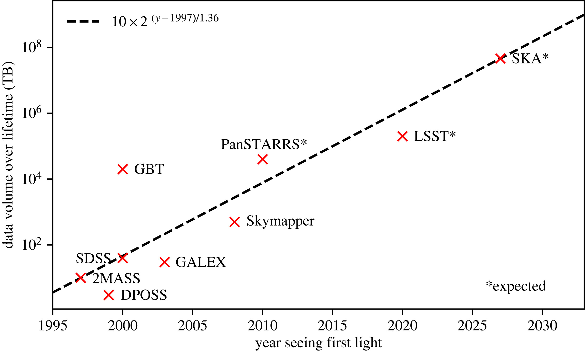
Over the past few decades, large-scale photometric surveys have transformed time-domain astronomy, providing vast, multi-wavelength datasets that are readily accessible through online databases. These surveys have been essential in detecting and classifying variable stars, discovering exoplanets, and identifying transient astronomical events. As shown in Figure 1, the data volume from astronomical surveys has grown exponentially, approximately doubling every 16 months. The combination of different survey datasets enables comprehensive studies of stellar variability across various timescales and wavelengths, driving both traditional astrophysical research and modern ML applications.
Photometric surveys can be broadly categorized into ground-based and space-based missions. Ground-based surveys provide wide-field and high-cadence monitoring, often covering extensive regions of the sky over long time periods. In contrast, space-based missions offer high-precision, uninterrupted observations unaffected by atmospheric distortions, enabling the detection of minute variations in stellar brightness.
Table LABEL:table1 provides an overview of major ground-based and space-based photometric surveys, including their active years, observed bands, sky coverage, and references.
2.1 Ground-based Observatories
Ground-based photometric surveys have significantly expanded understanding of stellar variability, exoplanetary systems, and the dynamic nature of the night sky. Through wide-field imaging and long-term monitoring, these surveys detect brightness variations in stars, uncovering key processes involved in stellar evolution. Covering different sky regions and wavelength bands, they provide extensive datasets that support various astrophysical studies. Below, ground-based observatories are grouped based on their primary target regions.
-
•
All-sky: ASAS, ROTSE, WASP, WISE, ASAS-SN
-
•
Milky Way (MW): MACHO, OGLE, UKIDSS
-
•
Wide field: LINEAR, CRTS, HATnet, VVV, HiTS, NGTS, Pan-STARRS, WFST, Rubin Obs.
-
•
Northern sky: NSVS, ZTF
-
•
Stripe 82: SDSS
2.2 Space-based Missions
Space-based photometric surveys have revolutionized precision astronomy by eliminating atmospheric distortions and enabling uninterrupted observations. These missions provide stable, high-sensitivity measurements, allowing for the detection of minute brightness variations in stars. Their contributions extend beyond exoplanet discovery to studies of stellar oscillations, galaxy evolution, and cosmic distance measurements. The extensive datasets from these surveys not only refine astrophysical models but also support ML applications in time-series analysis, enabling automated classification of variable stars, exoplanets, and other celestial phenomena. Below, space-based observatories are grouped based on their primary target regions.
-
•
All sky: Hipparcos, Gaia, TESS
-
•
Milky Way (MW): CoRoT, Kepler
-
•
Wide field: PLATO, ULTRASAT, Roman ST
-
•
Targeted field: JWST
| Surveys | Active years | Bands | Area | Reference |
|---|---|---|---|---|
| Hipparcos / Tycho | 1989-1993 | , | MW | Perryman et al. (1997); Høg et al. (1997) |
| MAssive Compact Halo Objects (MACHO) | 1992-1999 | V, R | MW, LMC, SMC | Alcock et al. (2000) |
| Optical Gravitational Lensing Experiment (OGLE) | 1992-present | V, I | MW, LMC, SMC | Udalski et al. (2015) |
| All Sky Automated Survey (ASAS) | 1997-present | V, I | All sky | Pojmanski (1997) |
| Two Micron All-Sky Survey (2MASS) | 1997-2001 | J, H, | All sky | Skrutskie et al. (2006) |
| Lincoln Near-Earth Asteroid Research (LINEAR) | 1998-2015 | Unfiltered | Wide field | Stokes et al. (2000) |
| Robotic Optical Transient Search Experiment (ROTSE) | 1998-present | Unfiltered | All sky | Akerlof et al. (2003) |
| Sloan Digital Sky Survey (SDSS) | 1998-present | u, g, r, i, z | Stripe 82 | York et al. (2000) |
| Northern Sky Variability Survey (NSVS) | 1999-2004 | Unfiltered | Northern sky | Woźniak et al. (2004) |
| Catalina Real-Time Survey (CRTS) | 2003-present | V | All sky | Drake et al. (2009) |
| Hungarian Automated Telescope Network (HATnet) | 2003-present | r | Wide field | Bakos et al. (2004) |
| Wide Angle Search for Planets (WASP / SuperWASP) | 2004-present | Optical | All sky | Pollacco et al. (2006) |
| UKIRT Infrared Deep Sky Survey (UKIDSS) | 2005-2014 | Z, Y, J, H, K | Wide field | Lawrence et al. (2007) |
| Convection, Rotation and Planetary Transits (CoRoT) | 2006-2013 | Unfiltered | MW | Barge et al. (2008) |
| Kepler mission | 2009-2018 | Unfiltered | MW | Koch et al. (2010) |
| Wide field Infrared Survey Explorer (WISE) | 2009-present | , , , | Wide field | Wright et al. (2010) |
| VISTA Variables in the Vía Láctea (VVV) | 2010-2016 | Z, Y, J, H, | Wide field | Minniti et al. (2010) |
| High Cadence Transit Survey (HiTS) | 2013-2015 | u, g, r, i | Wide field | Förster et al. (2016) |
| Gaia | 2013-present | BP, RP | All sky | Prusti et al. (2016) |
| All Sky Automated Survey for SuperNovae (ASAS-SN) | 2014-present | V, g | All sky | Kochanek et al. (2017) |
| Next Generation Transit Survey (NGTS) | 2015-present | I | Wide field | Wheatley et al. (2018) |
| Panoramic Survey Telescope and Rapid Response System (Pan-STARRS) | 2010-present | g, r, i, z, y | Wide field | Magnier et al. (2013) |
| Transiting Exoplanet Survey Satellite (TESS) | 2018-present | TESS-band | All sky | Ricker et al. (2015) |
| Zwicky Transient Facility (ZTF) | 2018-present | g, r, i | Northern sky | Bellm et al. (2018) |
| James Webb Space Telescope (JWST) | 2021-present | IR | Targeted fields | Gardner et al. (2023) |
| Wide Field Survey Telescope (WFST) | 2023-present | u, g, r, i, z, w | Northern sky | Lou et al. (2016) |
| Vera C. Rubin Observatory (formerly LSST) | 2025 (expected) | u, g, r, i, z, y | Wide field | Ivezić et al. (2019) |
| PLAnetary Transits and Oscillations of Stars (PLATO) | 2026 (expected) | B, V, R, I | Wide field | Rauer et al. (2014) |
| Ultraviolet Transient Astronomy Satellite (ULTRASAT) | 2027 (expected) | NUV | All sky | Shvartzvald et al. (2024) |
| Roman Space Telescope (formerly WFIRST) | 2027 (expected) | IR | Wide field | Spergel et al. (2015) |
3 Machine learning fundamentals
To demonstrate the applications of ML in LC analysis, this section provides a concise overview of core ML concepts.
ML enables systems to autonomously learn patterns from data and improve decision-making through experience, mirroring aspects of human cognition. Unlike traditional astronomical programming, which relies on explicit physical rules, ML algorithms derive implicit relationships directly from observational data. This data-driven approach offers flexibility for solving complex, nonlinear problems that defy conventional analytical methods Rodr´ıguez et al. (2022); Kembhavi & Pattnaik (2022); Sen et al. (2022).
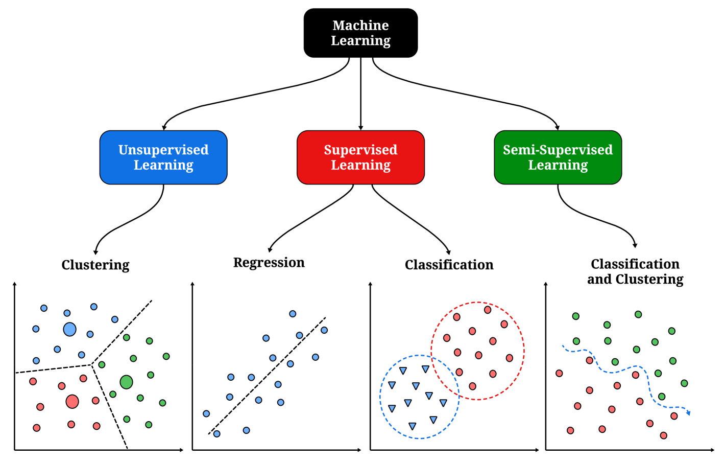
ML algorithms can be broadly categorized into supervised and unsupervised methods, often referred to as predictive and descriptive, respectively. These approaches may also be combined to form semi-supervised methods. Figure 2 provides a visual taxonomy of these approaches. Supervised algorithms learn mappings between input features and predefined target variables using labeled training data curated by domain experts (see e.g., Connolly et al. (1995); Collister & Lahav (2004); Reis et al. (2018a); Daniel et al. (2011); Fiorentin et al. (2007); Richards et al. (2012); Laurino et al. (2011); Masci et al. (2014); Morales-Luis et al. (2011); Bloom et al. (2012); Djorgovski et al. (2016); Mahabal et al. (2008); Miller (2015); Brescia et al. (2012); Krone-Martins et al. (2014); Wright et al. (2015); Lochner et al. (2016); D’Isanto et al. (2016); Castro et al. (2017); Naul et al. (2018); Ishida et al. (2019); D’Isanto & Polsterer (2018); Zucker & Giryes (2018); Delli Veneri et al. (2019); Krone-Martins et al. (2018); Mahabal et al. (2019); D’Isanto et al. (2018); Norris et al. (2019)). Unsupervised methods, conversely, autonomously identify hidden structures or relationships within unlabeled datasets. These techniques are typically divided into three subcategories: clustering (grouping similar data points), dimensionality reduction (extracting salient features), and anomaly detection (identifying outliers) (e.g., Boroson & Green (1992); D’Abrusco et al. (2009); Protopapas et al. (2006); Vanderplas & Connolly (2009); Ascasibar & Sánchez Almeida (2011); Almeida et al. (2010); D’Abrusco et al. (2012); Meusinger et al. (2012); Krone-Martins & Moitinho (2014); Fustes et al. (2013); Baron et al. (2015); Hocking et al. (2015); Nun et al. (2016); Gianniotis et al. (2016); Baron & Poznanski (2017); Reis et al. (2018b, c)). Anomaly detection holds particular promise for astronomical research, as it enables discovery of rare or unexpected phenomena within existing observational datasets.
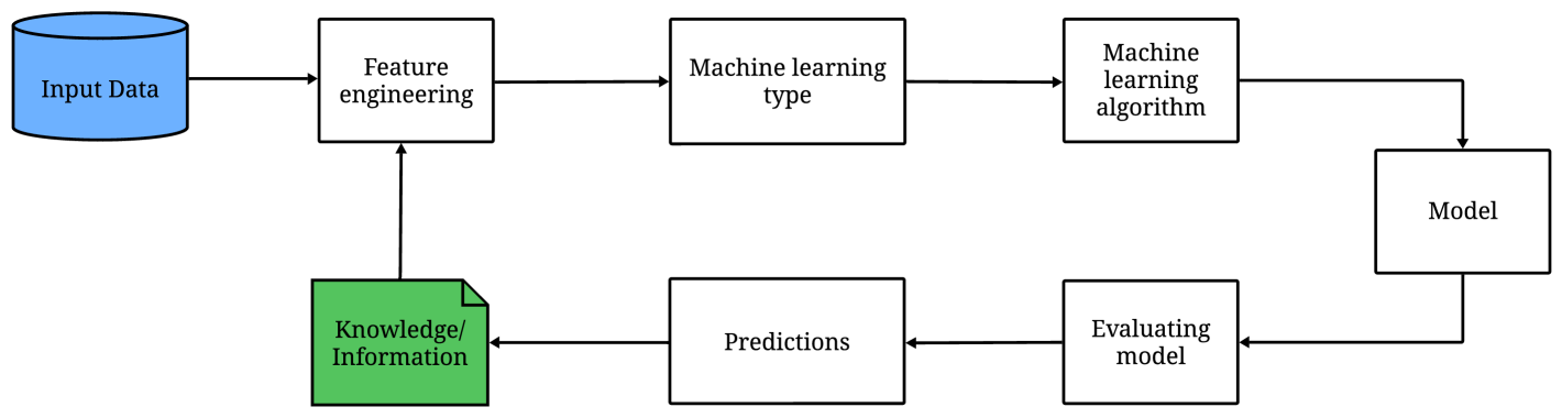
As an interdisciplinary field, ML integrates principles from statistics, optimization theory, and information science. Its primary focus lies in developing adaptive systems that simulate human learning processes to iteratively acquire knowledge, refine skills, and optimize performance. Figure 3 illustrates the iterative workflow of a typical ML system.
3.1 Supervised Learning
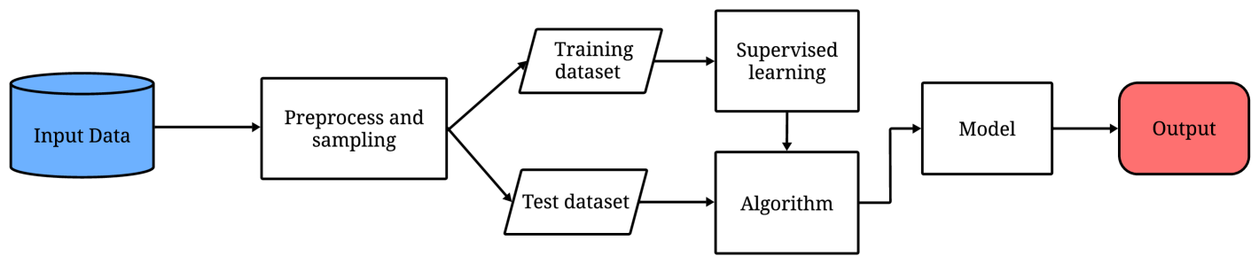
Supervised Learning (SL) operates under guidance, where labeled data provides the necessary supervision for model training. In this framework, class labels act as a reference, enabling the model to learn mappings between inputs and outputs. For instance, in a classification task, such as diagnosing a disease as positive or negative, the algorithm relies on predefined labels to make informed predictions. However, SL is inherently task-specific, meaning the model is limited to learning patterns strictly within the provided data and cannot generalize beyond its training scope Bishop & Nasrabadi (2006). The basic flow of SL is shown in Figure 4.
These algorithms optimize their performance by minimizing a cost function, which quantifies the discrepancy between predicted and actual values. The greater the deviation, the more challenging it becomes to achieve accurate predictions. Effective learning depends on a well-curated dataset with precise class labels, as a larger and higher-quality training set facilitates smoother optimization and improves model accuracy.
Decision tree is a non-parametric model built during training, represented as a top-down, tree-like structure. It is used for both classification and regression tasks. The tree consists of sequential nodes, where each node applies a condition to a specific feature in the dataset, guiding the decision-making process Quinlan (1986).
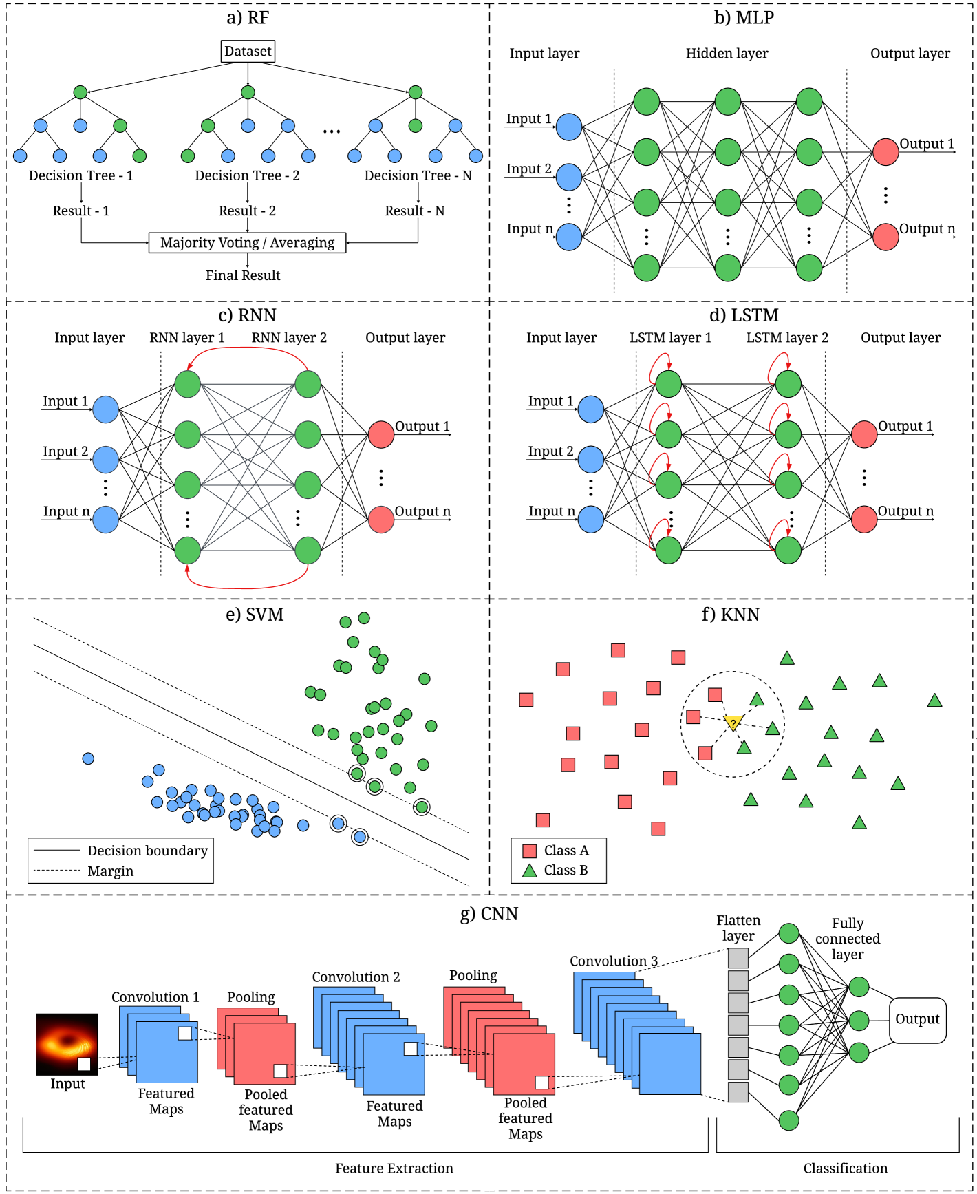
Random Forest (RF) is an ensemble learning method composed of multiple decision trees, where each tree is trained on a randomly selected subset of the training data and features Breiman (2001). This randomness reduces correlation between trees, enhancing generalization and robustness. Additionally, RF has relatively few hyper-parameters, making it an efficient and widely used ML model. Figure 5(a) illustrates a simple algorithm of RF.
Naive Bayes is a classification method based on Bayes’ theorem, assuming conditional independence of features given the target class Friedman et al. (1997). It estimates class probabilities using conditional probability formulas and assigns samples to the most probable class. Bayesian regression, in contrast, applies Bayesian inference to regression problems by modeling parameter distributions instead of single estimates, capturing uncertainty in predictions. Both methods leverage Bayesian principles, making them effective for probabilistic modeling in ML.
Artificial Neural Network (ANN) is a nonlinear, adaptive computational model designed to process information through a network of interconnected processing units Haykin (1994). Inspired by biological neural networks, ANNs simulate learning and decision-making by adjusting connections based on input data, making them highly effective for complex pattern recognition and predictive modeling in distributed environments.
Multilayer Perceptron (MLP) is a common type of ANN composed of multiple layers of fully connected neurons arranged hierarchically. It consists of an input layer, one or more hidden layers, and an output layer. Each neuron, or node, processes information using weighted connections and typically employs activation functions like sigmoid or ReLU to introduce non-linearity Pal & Mitra (1992). Figure 5(b) illustrates a typical MLP structure.
Recurrent Neural Network (RNN) is a type of ANN with recurrent connections, designed to model sequential data for recognition and prediction Bengio et al. (1994). It utilizes high-dimensional hidden states with nonlinear dynamics Sutskever et al. (2011), where each hidden state depends on its previous state Mikolov et al. (2014). This structure enables RNN to store, recall, and process complex temporal patterns over long durations, allowing it to map input sequences to output sequences and predict future time steps Salehinejad et al. (2017). Figure 5(c) illustrates a typical RNN structure.
Long Short-Term Memory (LSTM) is a specialized type of RNN designed to handle sequential data while overcoming the vanishing and exploding gradient problems. Unlike traditional RNNs, LSTMs use memory cells instead of standard hidden units, with gated mechanisms controlling input, output, and information flow. These gates help retain important features from previous time steps, enabling LSTMs to effectively capture long-term dependencies and improve sequence modeling Hochreiter & Schmidhuber (1997); Le et al. (2015); Gers et al. (2000). Figure 5(d) illustrates a typical LSTM structure.
Support Vector Machine (SVM) is a widely used SL algorithm applied in various astronomical tasks (e.g., Kovács & Szapudi (2015); Krakowski et al. (2016); Hartley et al. (2017); Hui et al. (2018); Ksoll et al. (2018); Pashchenko et al. (2018)). It identifies an optimal hyperplane in an -dimensional space to separate classes. In two dimensions, this hyperplane is a line dividing the plane so that each class falls on a different side. The optimal hyperplane maximizes the margin—the distance between the plane and the closest data points, known as support vectors. Once determined, the hyperplane acts as a decision boundary for classifying new data. Figure 5(e) illustrates an SVM hyperplane for a linearly separable two-dimensional dataset.
-Nearest Neighbors (KNN) is a non-parametric, instance-based learning algorithm used for classification and regression. Unlike most supervised methods that build predictive models, KNN directly stores training data and makes predictions by measuring similarity between data points. It calculates distances between a query point and all training samples, selecting the closest neighbors to determine the output Mucherino et al. (2009); Keller et al. (1985). As a lazy learner, KNN requires no explicit training phase but can be computationally expensive for large datasets due to pairwise distance calculations. Figure 5(f) illustrates a typical KNN structure.
Convolutional Neural Network (CNN) is a specialized DL architecture designed for processing structured grid-like data, such as images and time series. Unlike MLPs, which use fully connected layers throughout, CNNs employ convolutional layers that apply learnable filters to small regions of the input, capturing spatial hierarchies and local patterns. These layers reduce the number of parameters while preserving essential features, making CNNs efficient for feature extraction. Pooling layers further refine representations by reducing spatial dimensions, enhancing robustness to variations in input. Fully connected layers at the network’s end aggregate extracted features for final classification or regression tasks Li et al. (2021); O’shea & Nash (2015); Yamashita et al. (2018). Figure 5(g) illustrates a typical CNN structure.
3.2 Unsupervised Learning
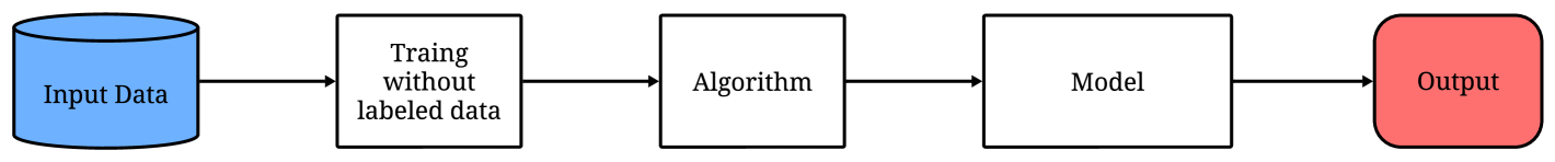
Unsupervised Learning (UL) is a ML approach that trains on unlabeled data, identifying underlying patterns and structures without predefined labels. Unlike supervised methods, which rely on labeled examples, unsupervised algorithms autonomously detect relationships, group similar data points, and uncover anomalies without external guidance. The basic flow of UL is shown in Figure 6.
UL encompasses a broad range of statistical techniques for data exploration, including clustering, dimensionality reduction, visualization, and anomaly detection. These methods are especially valuable in scientific research, as they enable the discovery of hidden patterns and the extraction of new insights from large datasets.
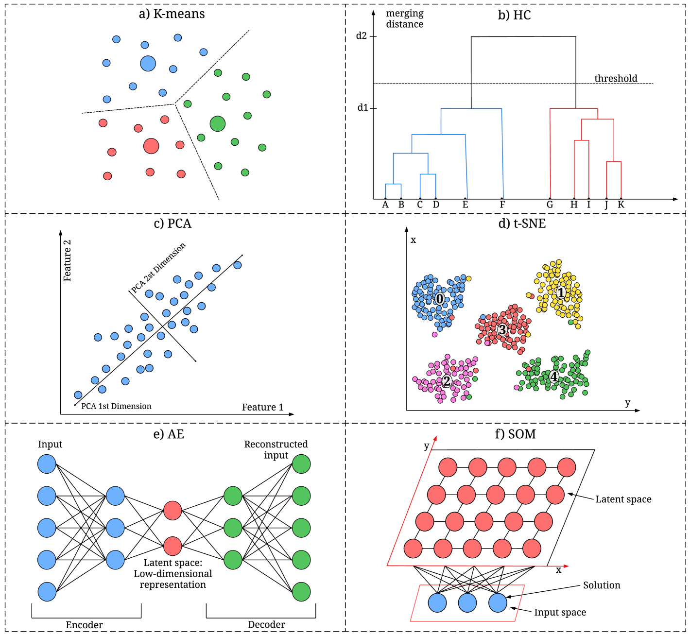
K-means is a widely used and well-known clustering algorithm valued for its simplicity and efficiency. It groups data points into distinct clusters based on their similarities by minimizing the variance within each cluster. The algorithm begins by randomly initializing cluster centroids, then assigns each data point to the nearest centroid based on a chosen distance metric, typically Euclidean distance. After assignment, the centroids are updated by computing the mean of all points within each cluster. This process iterates until convergence, which occurs when the centroid positions stabilize or a predefined iteration limit is reached MacQueen (1967); Hartigan & Wong (1979); Sinaga & Yang (2020). Figure 7(a) illustrates how K-means works, showing the iterative process of centroid updates and cluster assignments.
Hierarchical clustering (HC) is another popular clustering algorithm that aims to build a hierarchy of clusters Ward Jr (1963). There are two main types of HC: Agglomerative Hierarchical Clustering (AHC) and Divisive Hierarchical Clustering (DHC). AHC, also known as the ”bottom-up” approach, starts with each data point as an individual cluster and iteratively merges the closest clusters based on a chosen distance metric until it forms one cluster consisting of all data points. In contrast, DHC, referred to as the ”top-down” approach, begins with all data points grouped into a single cluster and recursively splits them into smaller clusters until each point becomes its own cluster Murtagh & Contreras (2012); Johnson (1967). Figure 7(b) illustrates AHC, showing the process of merging clusters in a ”bottom-up” manner.
Principal Component Analysis (PCA) is a widely used dimensionality reduction technique that transforms high-dimensional data into a lower-dimensional representation while retaining as much relevant information as possible Wold et al. (1987). It achieves this by identifying and projecting the data onto a set of orthogonal directions, known as principal components, which capture the maximum variance in the dataset. This transformation not only reduces the number of features but also mitigates the curse of dimensionality, enhances computational efficiency, and improves data interpretability by focusing on its most informative aspects Abdi & Williams (2010); Jolliffe & Cadima (2016). Figure 7(c) demonstrates the process of PCA.
t-Distributed Stochastic Neighbor Embedding (t-SNE) is another dimensionality reduction technique primarily used for visualization of high-dimensional data in two or three dimensions Van der Maaten & Hinton (2008). The algorithm represents each high-dimensional object as a two or three dimensional point, ensuring that similar objects are placed close together, while dissimilar objects are positioned farther apart with high probability. Unlike linear methods such as PCA, t-SNE captures non-linear relationships, making it particularly effective for revealing clusters and intricate patterns in complex datasets Van Der Maaten (2014); Kobak & Berens (2019). Figure 7(d) illustrates the t-SNE process.
Autoencoder (AE) is an ANN designed to learn efficient low-dimensional representations of input data, commonly used for tasks like compression, dimensionality reduction, and visualization Yang & Li (2015); Gianniotis et al. (2015, 2016). It consists of two main components: an encoder and a decoder. The encoder compresses the input data into a lower-dimensional representation, often referred to as the latent space, while the decoder reconstructs the original data from this compressed form. During training, the network optimizes its weights by minimizing the reconstruction error, typically measured as the squared difference between the input and the reconstructed output. Once trained, the bottleneck layer of the encoder provides a compact representation of the data, enabling its use in reduced-dimensional spaces for analysis or visualization. Figure 7(e) shows the structure of an AE.
Self-organizing map (SOM), also known as a Kohonen map Kohonen (1982), is an unsupervised ANN that creates a low-dimensional, typically two-dimensional, representation of high-dimensional input data. During training, the map self-organizes to closely match the topology of the input dataset, preserving its structure. In astronomy, SOMs have been applied for tasks such as semi-supervised classification, regression, clustering, visualization of complex datasets, and outlier detection (e.g., Armstrong et al. (2015, 2016); Meusinger et al. (2017); Rahmani et al. (2018)). Unlike traditional neural networks, where weights are used to transform input values through activation functions, the weights in SOMs represent the coordinates of the output neurons in the input data space. These weight vectors act as prototypes or templates, capturing the essential features of the input dataset. This unique structure allows SOMs to effectively map and visualize high-dimensional data in a more interpretable, lower-dimensional form. Figure 7(f) illustrates the SOM process.
3.3 Semi-supervised Learning
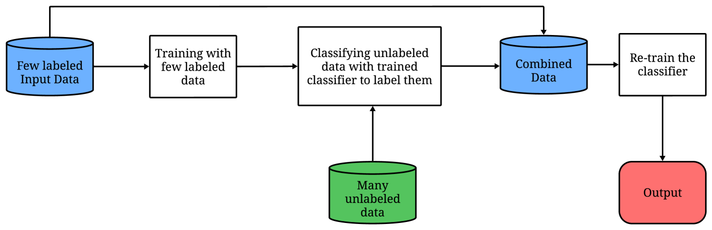
Semi-supervised learning (SSL) is a ML approach that integrates elements of both SL and UL. It leverages a small amount of labeled data alongside a large pool of unlabeled data, making it particularly useful when labeled data is scarce but unlabeled data is abundant Chapelle et al. (2009).
The SSL process begins with dataset collection, comprising both labeled and unlabeled data, followed by cleaning and preprocessing to ensure consistency. The model is initially trained on the labeled data to establish a foundational understanding of the task. It then refines its performance by incorporating information from the unlabeled data, improving overall accuracy. The general workflow of SSL is illustrated in Figure 8.
SSL can be categorized into inductive and transductive learning methods Van Engelen & Hoos (2020). Inductive learning aims to develop a generalized model capable of making predictions on unseen data. It utilizes both labeled and unlabeled data during training to enhance generalization. In contrast, transductive learning focuses on predicting labels solely for the specific unlabeled data available during training, without aiming for broader generalization. Transductive methods often exploit the inherent structure of the unlabeled data, such as relationships between data points, to improve prediction accuracy.
SSL offers several advantages, including more efficient data utilization by leveraging both labeled and unlabeled data, reducing the cost associated with manual labeling. Additionally, it enhances model performance by capturing structural patterns in unlabeled data. By bridging the gap between SL, which relies on labeled data, and UL, which identifies patterns without predefined labels, SSL provides a robust framework for learning in scenarios with limited labeled datasets.
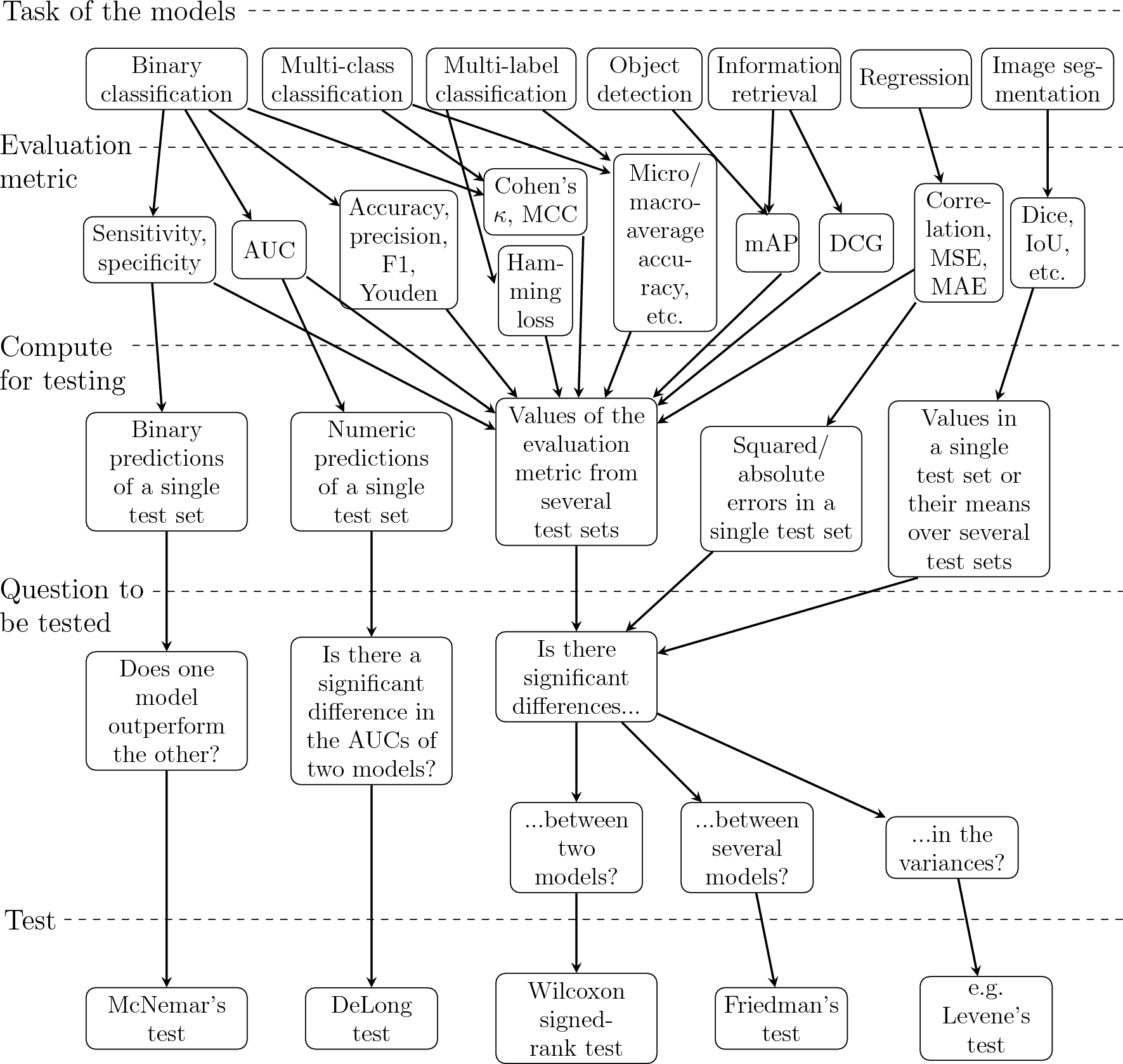
3.4 Evaluation Metrics
Evaluation metrics are essential tools in ML that quantitatively assess a model’s performance. They play a crucial role in optimizing hyper-parameters, evaluating model effectiveness, selecting the most relevant features, and comparing different ML algorithms. These metrics are computed during both the validation and testing phases, where the trained model is applied to previously unseen data, and its predictions are compared against actual target values to measure accuracy and reliability.
Different evaluation metrics are used depending on the specific task, ensuring that models are assessed appropriately based on their objectives. Figure 9, taken from Rainio et al. (2024), provides a comprehensive overview of evaluation metrics for various ML scenarios, detailing the tasks they address, the values that must be computed for statistical testing, the potential questions these tests can answer, and the appropriate statistical tests for each case.
4 Applications of Machine Learning in Light Curve Analysis
The increasing data volume from large-scale astronomical surveys such as Kepler, TESS, and the upcoming LSST presents both unprecedented opportunities and significant challenges in processing and interpretation. Traditional methods struggle with the scale, complexity, and noise in LC data, making automation essential. ML has emerged as a transformative approach, enabling efficient classification, detection, and characterization of astronomical objects with remarkable accuracy.
ML techniques are particularly effective at handling the high-dimensionality and noise inherent in LC data. By leveraging SL, UL, and SSL algorithms, ML facilitates pattern recognition, object classification, and anomaly detection with greater efficiency and precision than traditional methods. This section explores three pivotal applications of ML in LC analysis: (1) exoplanet detection, (2) variable star analysis, and (3) supernova classification.
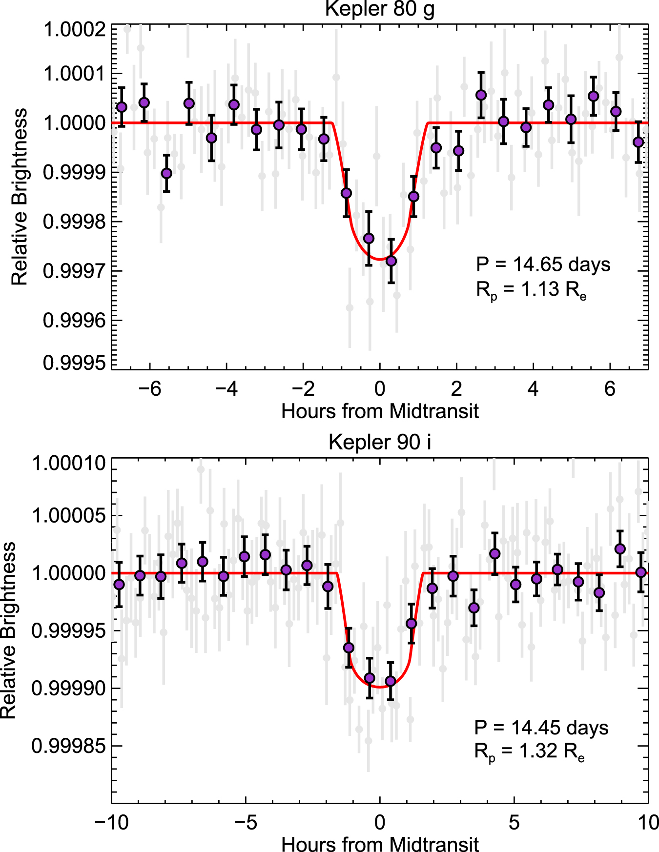
4.1 Transiting Exoplanet Detection
Transit photometry has become a fundamental technique for exoplanet discovery, detecting exoplanets by identifying periodic dips in a star’s brightness and serving as a cornerstone of modern planet-hunting surveys. Figure 10 illustrates a typical LC with a transit event, showcasing the subtle flux dip that ML algorithms are trained to recognize.
Space-based missions including Kepler (2009-2018) and TESS (2018-present) have revolutionized this field by providing high-precision photometric data across large sky areas. The Kepler mission identified thousands of planetary candidates through continuous monitoring of a single field, while TESS has expanded this catalog using its all-sky survey strategy focused on brighter stars. The analysis of these datasets presents significant computational challenges due to their volume, noise characteristics, and the presence of astrophysical false positives, necessitating advanced analytical approaches. Table LABEL:table2 presents a summary of ML methods applied to different exoplanet detection datasets.
The Kepler mission data have served as a testbed for developing ML techniques in transit detection. Initial work established the effectiveness of CNNs through the AstroNet architecture Shallue & Vanderburg (2018), which achieved classification performance comparable to human experts. Subsequent developments introduced modifications such as ExoNet Ansdell et al. (2018), incorporating additional diagnostic information to reduce false positives, and AstroNet-K2 Dattilo et al. (2019), adapted for the modified observing strategy of the K2 mission. Alternative approaches including 2D-CNN architectures Chintarungruangchai & Jiang (2019) and ensemble methods Priyadarshini & Puri (2021) demonstrated improved sensitivity to low signal-to-noise transits.
Analysis of TESS data has built upon these foundations while addressing the mission’s distinct characteristics. Modified versions of the original AstroNet framework have been applied to TESS observations Yu et al. (2019), with subsequent refinements such as Astronet-Triage-v2 Tey et al. (2023) improving classification accuracy. The Nigraha pipeline Rao et al. (2021) represents a comprehensive implementation integrating multiple analysis stages, while systems like SHERLOCK Dévora-Pajares et al. (2024) provide end-to-end processing capabilities. The ExoMiner Valizadegan et al. (2022) and its enhanced version ExoMiner++ Valizadegan et al. (2025) have demonstrated the potential of DL to replicate and augment expert vetting processes.
ML applications have been successfully adapted to various astronomical surveys and simulated datasets beyond the primary space-based missions. In simulated LC analysis, CNNs were applied to detect transits of habitable planets in high-cadence data Zucker & Giryes (2018), while alternative approaches included 1D CNNs for processing non-phase-folded LCs Iglesias Álvarez et al. (2023). GPU-accelerated phase-folding algorithms were developed specifically for detecting ultrashort-period exoplanets Wang et al. (2024).
For ground-based surveys, different ML approaches were implemented: RF and SOM techniques were combined in the NGTS survey for candidate vetting Armstrong et al. (2018), and CNNs were employed for automated candidate screening Chaushev et al. (2019). The QES project utilized DBSCAN-based algorithms for effective noise rejection in transit data Mislis et al. (2018). Similarly, the WASP survey integrated RF and CNN methods for comprehensive transit signal analysis Schanche et al. (2019).
CNNs were also implemented for the BRITE mission’s photometric data analysis Yeh & Jiang (2020). For infrared observations, LSTM networks were applied to Spitzer data for improved detrending of LCs Morvan et al. (2020). In Gaia photometry, XGBoost-assisted methods were developed for transit searches, leading to confirmed exoplanet discoveries Panahi et al. (2022).
These diverse applications demonstrate the versatility of ML techniques across various observational platforms, data types, and specific scientific requirements. The systematic development of analysis methods, reflects the ongoing evolution of techniques to address the challenges posed by current and future transit surveys. These methodological advances continue to enhance the detection and characterization of exoplanetary systems across diverse observational datasets.
| Data type | Method | Description |
|---|---|---|
| Kepler | CNN | Pearson et al. (2018) proposed a CNN-based method for exoplanet detection, outperforming least-squares techniques without requiring model fitting. |
| Shallue & Vanderburg (2018) developed AstroNet, a deep CNN designed for exoplanet classification. | ||
| Ansdell et al. (2018) proposed ExoNet, extending AstroNet by incorporating domain knowledge, centroid time-series data, and stellar parameters. | ||
| Dattilo et al. (2019) proposed AstroNet-K2, an extension of AstroNet adapted for Kepler’s K2 data. | ||
| Chintarungruangchai & Jiang (2019) proposed a 2D-CNN model with phase-folding for transit detection, demonstrating improved accuracy at low S/N. | ||
| Priyadarshini & Puri (2021) proposed an Ensemble-CNN model for exoplanet detection, comparing its performance with various ML algorithms. | ||
| Bugueño et al. (2021) proposed a CNN-based exoplanet detection method using MTF to transform unevenly sampled LCs into fixed-size images. | ||
| Cuéllar et al. (2022) proposed a CNN-based transit detection model trained on mixed real and synthetic data. | ||
| RF | Jenkins et al. (2012) proposed a RF-based approach to automate transit signal classification, generating a preliminary list of planetary candidates. | |
| McCauliff et al. (2015) expanded RF-based exoplanet classification by transforming transit-like detections into numerical attributes. | ||
| Sturrock et al. (2019) developed an RF-based exoplanet classification model and deployed it as a publicly accessible API in the cloud. | ||
| Caceres et al. (2019) developed the ARPS method combining ARIMA modeling, transit comb filtering, and RF classification to identify exoplanet candidates. | ||
| Jin et al. (2022) optimized SL with feature selection and tuning, with RF performing best, and used clustering to identify potentially habitable exoplanets. | ||
| Hesar & Foing (2024) evaluated six classification algorithms for exoplanet detection, identifying RF and SVM as the top performers based on accuracy and F1 score. | ||
| KNN | Thompson et al. (2015) proposed a ML-based metric using dimensionality reduction and KNN to identify transit-shaped signals. | |
| Bahel & Gaikwad (2022) explored exoplanet detection using ML classification, applying KNN on SMOTE-balanced data. | ||
| Ensemble | Hesar et al. (2024) applied ML models to estimate stellar rotation periods, demonstrating that Voting Ensemble improves accuracy over traditional approaches. | |
| Luz et al. (2024) evaluated five Ensemble ML algorithms for exoplanet classification. | ||
| ANN | Kipping & Lam (2016) developed an ANN-based model to predict short-period transits likely to have additional planets. | |
| SOM | Armstrong et al. (2016) developed a SOM-based method for fast exoplanet candidate classification. | |
| GPC | Armstrong et al. (2021) proposed a GPC-based probabilistic planet validation method as an alternative to VESPA. | |
| LightGBM | Malik et al. (2022) proposed a ML approach using TSFresh-extracted features and a gradient boosting classifier for transit detection. | |
| GAN | Suresh et al. (2024) explored GAN-based data augmentation for exoplanet detection, showing comparable accuracy with synthetic data and improved performance. | |
| TESS | CNN | Yu et al. (2019) modified AstroNet for automated triage and vetting of TESS candidates. |
| Osborn et al. (2020) adapted ExoNet for TESS data, training on simulated LCs. | ||
| Rao et al. (2021) developed Nigraha, built upon AstroNet, a pipeline combining transit detection, supervised ML, and vetting. | ||
| Olmschenk et al. (2021) developed a CNN for efficient exoplanet transit detection, and identified 181 new exoplanet candidates. | ||
| Tey et al. (2023) developed Astronet-Triage-v2, built upon AstroNet, an improved neural network for exoplanet candidate triage. | ||
| Fiscale et al. (2023) demonstrated that combining transfer learning with regularization techniques significantly enhances CNN performance. | ||
| Liao et al. (2024) proposed a wavelet-transform-based LC representation and an improved Inception-v3 CNN. | ||
| Dévora-Pajares et al. (2024) proposed SHERLOCK, an end-to-end pipeline that enables efficient exoplanet searches. | ||
| DNN | Valizadegan et al. (2022) proposed ExoMiner, a DL classifier that mimics expert vetting for transit signals. | |
| Valizadegan et al. (2025) introduced ExoMiner++, an enhanced version of ExoMiner, improving transit signal classification by integrating transfer learning. | ||
| Transformer | Salinas et al. (2025) proposed a Transformer-based NN for exoplanet detection, identifying transit signals without phase folding or periodicity assumptions. | |
| Simulated data | CNN | Zucker & Giryes (2018) proposed a CNN-based approach to detect transits of habitable planets in simulated high-cadence LCs. |
| Iglesias Álvarez et al. (2023) developed a 1D CNN for detecting transits in non-phase-folded LCs. | ||
| Wang et al. (2024) proposed GPFC, a GPU-accelerated phase-folding algorithm for ultrashort-period exoplanet detection. | ||
| NGTS | RF and SOM | Armstrong et al. (2018) developed autovet, a ML pipeline, combining RFs and SOMs to rank planetary candidates with high accuracy. |
| CNN | Chaushev et al. (2019) applied a CNN for automated vetting of exoplanet candidates, reducing manual effort. | |
| QES | DBSCAN | Mislis et al. (2018) developed TSARDI, a DBSCAN-based UL algorithm for noise rejection in transit surveys. |
| WASP | RF and CNN | Schanche et al. (2019) developed a ML pipeline combining RFs and CNNs for automated vetting of transit signals. |
| BRITE | CNN | Yeh & Jiang (2020) applied CNNs to BRITE LCs for exoplanet transit detection. |
| Spitzer Space Telescope | LSTM | Morvan et al. (2020) proposed TLCD-LSTM, a probabilistic LSTM-based detrending method for transit LCs. |
| Gaia | XGBoost | Panahi et al. (2022) developed a ML-assisted transit search in Gaia photometry, leading to the first exoplanet detections by Gaia, confirmed as hot Jupiters via radial velocity measurements. |
4.2 Variable Star Analysis
Stellar variability is a fundamental characteristic observed in numerous stars across the optical band, manifesting as periodic, semi-regular, or completely irregular brightness fluctuations. Variable stars are broadly categorized into intrinsic and extrinsic variables based on the underlying mechanisms driving their luminosity variations.
| Variable star types | Abbreviation |
|---|---|
| Eclipsing binary: Algol type | EA |
| Beta type | EB |
| W Ursae Majoris type | EW |
| Ellipsoidal binaries | ELL |
| Long period variable | LPV |
| Mira | MIRA |
| RV Tauri | RV |
| W Virginis: period 8 d | CWA |
| period 8 d | CWB |
| RS Canum Venaticorum | RS |
| BY Draconis | BY |
| Population II Cepheid | PTCEPH |
| Delta Cepheid | DCEP |
| first overtone | DCEPS |
| multi-mode | CEP(B) |
| Delta Scuti | DSCT |
| low amplitude | DSCTC |
| Gamma Doradus | GDOR |
| B emission-line star | BE |
| Gamma Cassiopeiae | GCAS |
| Alpha Cygni | ACYG |
| Beta Cephei | BCEP |
| Alpha-2 Canum Venaticorum | ACV |
| RR Lyrae: RRab type | RRAB |
| RRC type | RRC |
| RRd type | RRD |
| Slowly pulsating B star | SPB |
Intrinsic variables experience genuine changes in luminosity due to internal physical processes, such as stellar pulsations, eruptions, or structural expansion and contraction. This category primarily includes pulsating and eruptive variables. Pulsating variables undergo periodic expansions and contractions in their outer layers, leading to observable brightness oscillations. Notable examples include Cepheids, RR Lyrae, and Mira variables, each exhibiting distinct pulsation periods and amplitude variations. Eruptive variables, such as cataclysmic variables and nova-like stars, exhibit sudden and often dramatic changes in brightness, typically due to stellar outbursts or accretion-related instabilities.
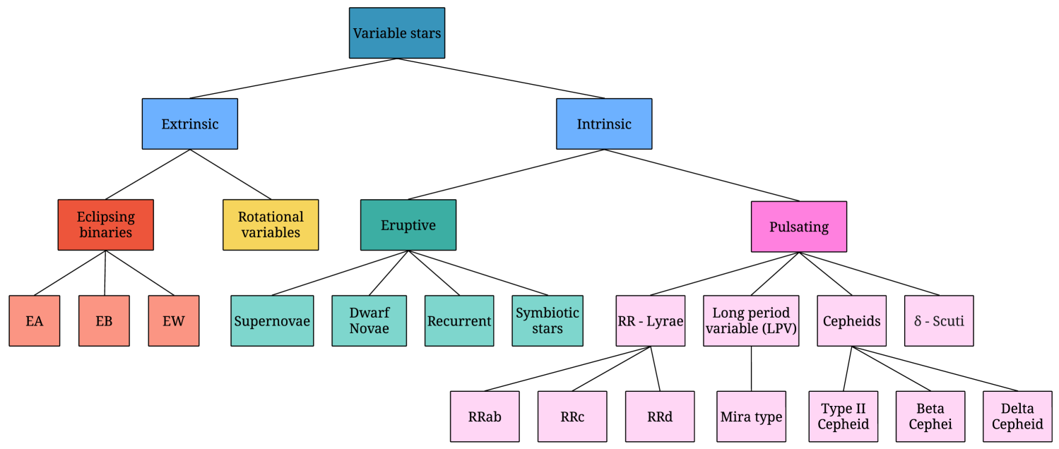
Extrinsic variables, in contrast, exhibit brightness fluctuations due to external factors, such as eclipses or rotational modulations. This category encompasses eclipsing binaries and rotating variables. Eclipsing binary systems consist of two or more gravitationally bound stars orbiting a common center of mass, where periodic eclipses result in characteristic minima in their LCs. The primary and secondary minima in their LCs provide insights into stellar radii, temperatures, and orbital inclinations. Rotating variables exhibit modest brightness variations arising from stellar surface features, such as starspots or ellipsoidal distortions, modulated by the star’s rotation.
Figure 11 presents a schematic classification of variable stars, while Table 3 lists their primary types and corresponding abbreviations. The analysis of variable star LCs plays a crucial role in distinguishing between different classes. Pulsating variables, for instance, exhibit smooth and regular brightness oscillations, whereas eclipsing binaries show well-defined periodic minima. These distinctions enable robust classification and facilitate astrophysical inferences about stellar structure, evolution, and binary interactions.
The systematic classification of variable stars relies heavily on distinguishing subtle features in their LCs, such as periodicity, amplitude, and morphological patterns. Traditional classification frameworks often depend on manually engineered features (e.g., periodograms, Fourier coefficients, or phased-folded curve statistics), which may fail to capture nuanced or non-linear relationships in large datasets. ML methods overcome these limitations by automating feature extraction and enabling robust classification across diverse variable star populations. Table LABEL:table4 provides a comprehensive summary of ML techniques applied to variable star analysis, reflecting the evolution of methodologies from early Bayesian approaches to modern DL architectures.
Early ML implementations focused on probabilistic methods and ensemble techniques. Bayesian Networks (BNs) and Gaussian Mixture Models (GMMs) were employed for CoRoT and Hipparcos datasets to probabilistically associate LC features with physical classes Debosscher et al. (2007); Sarro et al. (2006). The introduction of RFs marked a significant advancement, enabling feature importance analysis and improved handling of imbalanced datasets Richards et al. (2011a); Dubath et al. (2011). Subsequent hybrid approaches combined RFs with dimensionality reduction techniques like PCA or SOMs to enhance interpretability Armstrong et al. (2015); Rimoldini et al. (2012).
The advent of DL revolutionized variable star classification by leveraging raw or minimally preprocessed LCs. CNNs achieved state-of-the-art performance on surveys like CRTS and Kepler, identifying hierarchical patterns directly from flux measurements Mahabal et al. (2017); Akhmetali et al. (2024). RNNs and LSTM networks proved particularly effective for capturing temporal dependencies in irregularly sampled data from ASAS-SN and Gaia Naul et al. (2018); Merino et al. (2024). Transformer architectures, recently applied to Kepler and ZTF data, demonstrated superior performance in modeling long-range dependencies without phase-folding assumptions Pan et al. (2024); Cádiz-Leyton et al. (2024).
| Data type | Method | Description |
|---|---|---|
| ASAS | Bayesian Classifier | Eyer & Blake (2005) developed a Fourier-based Bayesian classifier for ASAS variables. |
| Hipparcos | Bayesian ensemble | Sarro et al. (2006) developed a Bayesian ensemble of neural networks for automatic classification of eclipsing binary LCs. |
| OGLE | BN and SVM | Debosscher et al. (2007) presented BN and SVM in the application of the methodology to variable stars. |
| OGLE | BN and SVM | Sarro et al. (2009) developed and tested a Fourier-based Bayesian classifier |
| CoRoT | BN and GMM | Debosscher et al. (2009) developed a fast pipeline for classifying CoRoT LCs and discovering new stellar variability types. |
| OGLE and Hipparcos | RF | Richards et al. (2011a) developed a ML methodology using RF. |
| Hipparcos | RF and BN | Dubath et al. (2011) evaluated automated classification of Hipparcos periodic stars using RFs. |
| Hipparcos | RF and BN | Rimoldini et al. (2012) applied RFs to classify periodic, non-periodic, and irregular Hipparcos variables. |
| Kepler | RF | Long et al. (2012) introduced noisification to reduce survey-dependent feature mismatch. |
| Hipparcos and OGLE | Active Learning (AL) | Richards et al. (2011b) used active learning to reduce sample bias in variable star classification |
| PTF | RF | Bloom et al. (2012) developed a ML framework for PTF to automate discovery and classification of transients and variables. |
| LINEAR | GMM and SVM | Sesar et al. (2013) proposed method for identifying visually confirmed variable stars within the LINEAR survey. |
| LINEAR | GMM and SVM | Palaversa et al. (2013) identified 7000 faint periodic stars using LINEAR and SDSS data. |
| MACHO | BN and RF | Nun et al. (2014) proposed methodology for anomaly detection in MACHO data. |
| WISE | RF and AL | Masci et al. (2014) proposed methodology for classifying periodic variable stars. |
| Catalogue of Eclipsing Variables | Membership probability | Avvakumova & Malkov (2014) developed a procedure to classify eclipsing binaries based on LC parameters. |
| OGLE and ASAS | KNN, SVM and RF | Kügler et al. (2015) proposed a density model for classifying irregular time-series data. |
| Kepler | SOM and RF | Armstrong et al. (2015) developed a novel method for classifying variable stars by combining SOM and RF. |
| Kepler | RF and BN | Bass & Borne (2016) proposed an ensemble approach for variable star classification in the Kepler field. |
| MACHO, LINEAR and ASAS | RF | Kim & Bailer-Jones (2016) developed a general-purpose ML package for classifying periodic variable stars. |
| MACHO and OGLE | SVM | Mackenzie et al. (2016) extracted subsequences of LCs and clustered them to identify common local patterns. |
| UCR and LINEAR | KNN, RF, RBF-NN | Johnston & Peter (2017) developed a novel time-domain feature extraction method called Slotted Symbolic Markov Modeling (SSMM). |
| ASAS, Hipparcos and OGLE | KNN, SVM, and RF | Johnston & Oluseyi (2017) proposed a method for classifying variable stars using supervised pattern recognition. |
| CRTS | CNN | Mahabal et al. (2017) developed a DL approach for classifying LCs by transforming sparse, irregular time-series data into 2D representation. |
| ASAS, LINEAR, MACHO | RNN | Naul et al. (2018) developed an unsupervised autoencoding RNN that effectively handles irregularly sampled, noisy LCs. |
| Kepler | LSTM and RNN | Hinners et al. (2018) presented methods for representation learning and feature engineering aimed at predicting and classifying properties. |
| OGLE | LR, SVM, KNN, RF, and SGB | Pashchenko et al. (2018) proposed a ML approach for variability detection. |
| OGLE, MACHO and Kepler | Fast Similarity Function | Valenzuela & Pichara (2018) presented a novel data structure called the Variability Tree. |
| Gaia and ASAS | RF | Jayasinghe et al. (2019) utilized the RF classifier along with a series of classification corrections. |
| OGLE, VISTA and CoRoT | CNN | Aguirre et al. (2019) developed a scalable CNN architecture for survey-independent LC classification. |
| ASAS-SN | RNN | Tsang & Schultz (2019) developed classifier combining an RNN AE with a GMM. |
| ASAS | PCA and RF | McWhirter et al. (2019) focused on processing time-series data with uneven cadence by leveraging representation learning to extract useful features. |
| CRTS | RF | Hosenie et al. (2019) developed an optimized ML framework for variable star classification. |
| Light curves in Galactic Plane | -medoids method | Modak et al. (2020) proposed a -medoids clustering approach to objectively classify galactic variable stars. |
| CoRoT, OGLE and MACHO | Streaming Probabilistic Model | Zorich et al. (2020) proposed a streaming probabilistic classification model that uses a novel set of features. |
| OGLE, Gaia and WISE | RNN | Becker et al. (2020) developed an end-to-end DL approach using RNNs for efficient variable star classification. |
| CRTS | RF and XGBoost | Hosenie et al. (2020) proposed a hybrid approach combining HC with data augmentation techniques. |
| MACHO | RNN | Jamal & Bloom (2020) conducted systematic comparison of neural network architectures for time-series classification. |
| UCR Starlight and LINEAR | Multi-View Metric Learning | Johnston et al. (2020) introduced a Multi-View Metric Learning framework that leverages multiple data representations. |
| OGLE | iTCN and iResNet | Zhang & Bloom (2021) developed Cyclic-Permutation Invariant Neural Networks that achieve state-of-the-art accuracy. |
| OGLE | CNN and LSTM | Bassi et al. (2021) proposed 1D CNN-LSTM hybrid network for direct variable star classification using raw time-series data. |
| Simulated data | LSTM | Čokina et al. (2021) developed a DL method for automated classification of eclipsing binaries. |
| ZTF | BRF | Sánchez-Sáez et al. (2021) introduced ALeRCE’s first LC classifier, a two-level balanced RF system processing ZTF alerts. |
| Kepler | GMM | Barbara et al. (2022) developed an interpretable classification system for Kepler LCs. |
| OGLE | Multiple-Input Neural Network | Szklenár et al. (2022) developed a Multiple-Input Neural Network combining CNNs and MLPs. |
| OGLE, CSS, Gaia | UMAP and HDBSCAN | Pantoja et al. (2022) developed semi-supervised and clustering-based approaches for variable star classification. |
| VVV | RF and XGBoost | Molnar et al. (2022) developed VIVACE, an automated two-stage classification pipeline. |
| ZTF | CVAE | Chan et al. (2022) proposed an unsupervised DL approach using variational AE and isolation forests. |
| Kepler | ResNet and LSTM | Yan et al. (2023) developed RLNet, a hybrid ResNet-LSTM neural network. |
| TESS | SVM | Elizabethson et al. (2023) developed a ML framework classifying T Tauri stars into 11 morphological classes. |
| Gaia | LSTM and GRU | Merino et al. (2024) proposed a self-supervised learning approach using RNNs. |
| LAMOST | LightGBM and XGBoost | Qiao et al. (2024) developed a LightGBM/XGBoost-based classification system for LAMOST DR9 data. |
| OGLE | CNN | Monsalves et al. (2024) developed an efficient CNN-based classification system using 2D histogram representations of OGLE LCs. |
| TESS | CNN | Olmschenk et al. (2024) developed a rapid CNN classifier for TESS 30-minute cadence data. |
| TMTS | XGBoost and RF | Guo et al. (2024) developed a classification system for TMTS variables using XGBoost and RF. |
| ZTF | Distance Metric Classifier | Chaini et al. (2024) developed DistClassiPy, an interpretable distance-metric classifier for variable stars. |
| MACHO, OGLE and ATLAS | Transformer | Cádiz-Leyton et al. (2024) proposed HA-MC Dropout, a novel transformer-based method combining hierarchical attention and Monte Carlo dropout. |
| Kepler | Transformer | Pan et al. (2024) developed Astroconformer, a Transformer- based model that demonstrates superior performance. |
| OGLE | CNN | Akhmetali et al. (2024) developed a CNN-based approach for automated variable star classification. |
4.3 Supernova classification
Supernovae (SNe) are among the most energetic transient phenomena in the universe. They play a critical role in stellar evolution, the chemical enrichment of the interstellar medium, and cosmological distance measurements. Their classification traditionally relies on spectroscopic and photometric observations. While spectroscopic classification remains the most accurate, it is expensive and has high requirements for telescopes and observation time, and thus cannot be applied to all observed transients.
Photometric classification, although less precise, offers higher observational efficiency and has gained importance with the advent of wide-field surveys. Early photometric methods used template fitting and parametric modeling of LCs, leveraging features such as peak brightness, decline rate, and color evolution. However, these methods typically require complete LCs with full phase coverage, limiting their application to real-time or sparsely sampled data.
Recent advances in ML have significantly enhanced SN classification capabilities, especially under constraints such as low signal-to-noise ratios and incomplete data. ML-based approaches can classify a wide range of transient types and support near real-time classification. This is critical for follow-up prioritization and maximizing the scientific return from transient surveys. Table 5 provides SN classes and their physical origins, while Table LABEL:table6 summarizes various ML methods applied to SN classification.
| Supernova types | Physical origin |
|---|---|
| SN Ia | White Dwarf |
| SN Ib | Massive star |
| SN Ic | Massive star |
| SN Ic-BL | Massive star |
| SN II | Massive star |
| SN IIb | Massive star |
| SN IIn | Massive star |
| SLSN | Massive star |
Early ML applications focused on engineered features derived from parametric LC fits or domain-specific metrics. The Supernova Photometric Classification Challenge (SNPCC) Kessler et al. (2010) was created as a standardized dataset to evaluate ML-based photometric classification methods for SN. Many subsequent studies tested their algorithms on the SNPCC dataset Newling et al. (2011); Richards et al. (2012); Karpenka et al. (2013); Gupta et al. (2016); Lochner et al. (2016); Charnock & Moss (2017); Ishida et al. (2019); Pasquet et al. (2019); Santos et al. (2020); de Oliveira et al. (2023).
DL revolutionized SN classification by allowing models to process raw flux measurements or minimally preprocessed LCs. Initial ML applications employed a variety of feature‐based techniques: Kernel Density Estimation (KDE) and Boosting methods Newling et al. (2011), Non‐linear Dimensionality Reduction with RFs Richards et al. (2012), ANNs Karpenka et al. (2013), Domain Adaptation with AL Gupta et al. (2016), and Naive Bayes, KNN, SVM, ANN, and BDTs Lochner et al. (2016).
RNN and CNN architectures then advanced photometric classification by ingesting raw time series directly. Deep RNNs (including LSTM variants) demonstrated strong performance on SNPCC and SALT2‐fitted LCs Charnock & Moss (2017); Möller & de Boissière (2020), while CNNs learned hierarchical features from 2D representations of LCs Brunel et al. (2019); Qu et al. (2021). Hybrid models, such as SuperNNova Möller & de Boissière (2020), SuperRAENN Villar et al. (2020), and PELICAN framework Pasquet et al. (2019) leveraged SSL and AEs to boost purity and completeness.
Recent classification pipelines increasingly incorporate generative models, Gaussian Process (GP) augmentation, and real-time alert systems. For example, the ParSNIP framework Boone (2021) utilizes Variational Autoencoders (VAEs) to perform classification. Similarly, Avocado Boone (2019) applies LightGBM combined with GP augmentation to classify transients photometrically. Real-time alert brokers like Fink Leoni et al. (2022) streamline the early identification of SNe from surveys like ZTF using AL strategies. CNN-based models such as SCONE Qu et al. (2021) apply 2D GP regression to multi-band LCs, while Photo-SNthesis Qu & Sako (2023) uses CNNs to generate full redshift probability distributions. Temporal convolutional networks (TCNs) paired with LightGBM, as in the TLW model Li et al. (2024), further demonstrate the effectiveness of hybrid architectures for robust, survey-independent transient classification.
| Data type | Method | Description |
|---|---|---|
| SNPCC | KDE and Boosting | Newling et al. (2011) proposed two classification methods for the application of SNPCC data. |
| SNPCC | Non-linear Dimension Reduction and RF | Richards et al. (2012) proposed the non-linear dimension reduction technique to detect structure in a data base of SNe LCs. |
| SNPCC | ANN | Karpenka et al. (2013) presented a method for automated photometric classification of SNe. |
| SNPCC | Domain Adaptation and AL | Gupta et al. (2016) presented an adaptive mechanism that generates a predictive model to identify SNe Ia. |
| SNPCC | Naive Bayesian, KNN, SVM, ANN and BDT | Lochner et al. (2016) developed a multi-faceted classification pipeline. |
| SNLS | XGBoost | Möller et al. (2016) presented a method to photometrically classify SNe Ia. |
| SNPCC | Deep RNN | Charnock & Moss (2017) presented deep RNN for performing photometric classification of SNe. |
| SNPCC | CNN | Brunel et al. (2019) presented CNN for SNe Ia classification. |
| SNPCC | AL | Ishida et al. (2019) developed a framework for spectroscopic follow-up design for optimizing supernova photometric classification. |
| PS1-MDS | SVM, RF and MLP | Villar et al. (2019) developed 24 classification pipelines with different feature extraction and data augmentation methods. |
| PLAsTiCC | DNN | Muthukrishna et al. (2019) developed RAPID, a novel time-series classication tool for identifying explosive transients. |
| PLAsTiCC | LightGBM | Boone (2019) developed Avocado, a software package for classification of transients with GP augmentation. |
| SNPCC | CNN and AE | Pasquet et al. (2019) developed PELICAN, an algorithm for the characterization and the classification of SNe LCs. |
| SALT2 fitted | RNN | Möller & de Boissière (2020) developed SuperNNova, a framework for photometric classification of SNe. |
| PS1-MDS | RF and RAENN | Villar et al. (2020) developed SuperRAENN, a semi-supervised SN photometric classification pipeline. |
| OSC and ZTF | RF | Gomez et al. (2020) developed a classification algorithm targeted at rapid identification of a pure sample of SLSN-I. |
| SNPCC | TPOT, XGBoost, AdaBoost, GBoost, EXT, RF | Santos et al. (2020) analyzed the performance of boosting and averaging methods for classification of SNe. |
| SALT2 | DNN | Takahashi et al. (2020) developed a classification algorithm to classify LCs observed by Subaru/HSC. |
| PS1-MDS | RF | Hosseinzadeh et al. (2020) developed Superphot, an open-source classification algorithm for photometric classification of SNe. |
| PS1-MDS and PLAsTiCC | VAE | Boone (2021) developed ParSNIP, a hybrid model to produce empirical generative models of transients from data sets of unlabeled LCs. |
| PLAsTiCC | CNN | Qu et al. (2021) developed SCONE, a CNN-based classification method using 2D GP regression. |
| PLAsTiCC | CNN | Qu & Sako (2022) presented classification results on early SNe LCs from SCONE. |
| ZTF | AL | Leoni et al. (2022) developed Fink, a broker for early SNe classification. |
| Open Supernova Catalog | GP | Stevance & Lee (2023) explored the application of GP to SNe LCs. |
| SNPCC | XGBoost | de Oliveira et al. (2023) developed a linear regression algorithm optimized through automated machine learning (AutoML) frameworks. |
| PLAsTiCC and ZTF | MLP, NF and Bayesian Neural Network | Demianenko et al. (2023) examined several ML-based LC approximation methods. |
| PLAsTiCC and Simulated SDSS-II SN data | CNN | Qu & Sako (2023) developed Photo-SNthesis, a CNN-based method for predicting full redshift probability distributions from multi-band SNe LCs. |
| ZTF | AL | Pruzhinskaya et al. (2023) explored the potential of AL techniques in application to detect new SNe candidates. |
| ZTF | LightGBM | de Soto et al. (2024) developed Superphot+, a photometric classifier for SNe LCs that does not rely on redshift information. |
| PLAsTiCC | TCN and LightGBM | Li et al. (2024) developed TLW, a classification algorithm for transients. |
5 Challenges and Open Issues
The application of ML to LC analysis has transformed astronomical research, yet several significant challenges remain in building robust, interpretable, and survey-independent classification systems. These challenges are expected to intensify with the data influx from next-generation surveys such as the LSST, which is projected to detect tens of millions of transient events each night.
A central difficulty lies in the heterogeneity and sparsity of data. Many surveys, including ASAS-SN and Gaia, produce LCs with irregular sampling due to observational constraints such as weather or scheduling. This irregularity poses challenges for the direct application of DL models, which are typically designed for regularly sampled data. Furthermore, models trained on data from one survey, such as Kepler, often fail to generalize to others like TESS, due to differences in cadence, noise properties, and photometric filters. The problem is compounded by the scarcity of high-quality labels, as spectroscopic confirmations are limited, especially for rare transient classes such as SLSNe.
Another major challenge involves the interpretability of ML models and their consistency with physical principles. ML models often function as black boxes, providing predictions without clear explanations. This lack of transparency limits their utility in cosmological studies that require rigorous uncertainty quantification and interpretability. There is a growing interest in hybrid approaches that combine data-driven learning with physics-based priors.
Real-time processing and early classification are also critical challenges. LSST’s alert stream will require sub-minute response times, which strain the capabilities of even highly optimized neural networks. Moreover, many existing classification techniques rely on full-phase LCs for accurate classification. In contrast, real-time systems must operate on partial data, often limited to early stages such as the rising or plateau phases of the LC. Developing models that can provide reliable early-time classifications is a key area of ongoing research.
Lastly, class imbalance and anomaly detection present persistent obstacles. Rare events such as kilonovae or luminious red novae are difficult to detect using standard classification methods. Traditional oversampling techniques are often insufficient for handling such imbalance, and alternative generative or data augmentation strategies are needed. In addition, most ML classifiers operate under a closed-set assumption, recognizing only a fixed set of known classes. However, LSST and similar surveys are expected to discover entirely new types of transients.
6 Conclusions
The rapid advancement of observational capabilities in astronomy has led to an exponential increase in the volume of LC data, opening up both exciting opportunities and complex challenges for time-domain astronomy. In this evolving landscape, ML has emerged as a powerful tool, finding applications across a broad spectrum of tasks. This review discusses major photometric surveys that provide the essential LC data, outlines the fundamental principles of ML, and explores ML applications in LC analysis, including exoplanet detection, variable star analysis, and supernova classification, highlighting the increasing sophistication and versatility of these methods.
As astronomical surveys scale up in depth, cadence, and volume, the need for automated, scalable, and interpretable analysis pipelines becomes ever more urgent. ML models, particularly DL architectures, have shown exceptional performance in handling large, noisy, and irregular datasets. Importantly, the choice of ML approach depends on the specific scientific goal, the nature of the dataset, and the balance among performance, interpretability, and computational cost. At the same time, critical challenges such as survey dependence, class imbalance, interpretability, and real-time applicability remain open issues.
Future advancements are likely to involve approaches that go beyond purely data-driven methods by integrating physical models, enhancing generalizability across different surveys, and incorporating robust uncertainty quantification.The convergence of domain expertise and machine intelligence holds the key to not only improving classification accuracy but also enabling new scientific insights.
In conclusion, the fusion of ML with astronomical time-series data is not just a technical advancement—it represents a paradigm shift in how discoveries are made. As datasets continue to expand, so too will the opportunities for ML to illuminate the dynamic universe in ways previously unimaginable.
References
- Abdi & Williams (2010) Abdi, H., & Williams, L. J. 2010, Wiley interdisciplinary reviews: computational statistics, 2, 433
- Aguirre et al. (2019) Aguirre, C., Pichara, K., & Becker, I. 2019, Monthly Notices of the Royal Astronomical Society, 482, 5078
- Ahuja et al. (2020) Ahuja, R., Chug, A., Gupta, S., Ahuja, P., & Kohli, S. 2020, Nature-inspired computation in data mining and machine learning, 225
- Akerlof et al. (2003) Akerlof, C., Kehoe, R., McKay, T., et al. 2003, Publications of the Astronomical Society of the Pacific, 115, 132
- Akhmetali et al. (2024) Akhmetali, A., Namazbayev, T., Subebekova, G., et al. 2024, Galaxies, 12, 75
- Alcock et al. (2000) Alcock, C., Allsman, R., Alves, D. R., et al. 2000, The Astrophysical Journal, 542, 281
- Almeida et al. (2010) Almeida, J. S., Aguerri, J. A. L., Munoz-Tunón, C., & De Vicente, A. 2010, The Astrophysical Journal, 714, 487
- Ansdell et al. (2018) Ansdell, M., Ioannou, Y., Osborn, H. P., et al. 2018, The Astrophysical journal letters, 869, L7
- Armstrong et al. (2021) Armstrong, D. J., Gamper, J., & Damoulas, T. 2021, Monthly Notices of the Royal Astronomical Society, 504, 5327
- Armstrong et al. (2016) Armstrong, D. J., Pollacco, D., & Santerne, A. 2016, Monthly Notices of the Royal Astronomical Society, stw2881
- Armstrong et al. (2015) Armstrong, D. J., Kirk, J., Lam, K., et al. 2015, Monthly Notices of the Royal Astronomical Society, 456, 2260
- Armstrong et al. (2018) Armstrong, D. J., Günther, M. N., McCormac, J., et al. 2018, Monthly Notices of the Royal Astronomical Society, 478, 4225
- Ascasibar & Sánchez Almeida (2011) Ascasibar, Y., & Sánchez Almeida, J. 2011, Monthly Notices of the Royal Astronomical Society, 415, 2417
- Avvakumova & Malkov (2014) Avvakumova, E., & Malkov, O. Y. 2014, Monthly Notices of the Royal Astronomical Society, 444, 1982
- Bahel & Gaikwad (2022) Bahel, V., & Gaikwad, M. 2022, in 2022 IEEE Region 10 Symposium (TENSYMP), IEEE, 1–5
- Bakos et al. (2004) Bakos, G., Noyes, R., Kovács, G., et al. 2004, Publications of the Astronomical Society of the Pacific, 116, 266
- Ball & Brunner (2010) Ball, N. M., & Brunner, R. J. 2010, International Journal of Modern Physics D, 19, 1049
- Barbara et al. (2022) Barbara, N. H., Bedding, T. R., Fulcher, B. D., Murphy, S. J., & Van Reeth, T. 2022, Monthly Notices of the Royal Astronomical Society, 514, 2793
- Barge et al. (2008) Barge, P., Baglin, A., Auvergne, M., et al. 2008, Astronomy & Astrophysics, 482, L17
- Baron (2019) Baron, D. 2019, arXiv preprint arXiv:1904.07248
- Baron & Poznanski (2017) Baron, D., & Poznanski, D. 2017, Monthly Notices of the Royal Astronomical Society, 465, 4530
- Baron et al. (2015) Baron, D., Poznanski, D., Watson, D., et al. 2015, Monthly Notices of the Royal Astronomical Society, 451, 332
- Bass & Borne (2016) Bass, G., & Borne, K. 2016, Monthly Notices of the Royal Astronomical Society, 459, 3721
- Bassi et al. (2021) Bassi, S., Sharma, K., & Gomekar, A. 2021, Frontiers in Astronomy and Space Sciences, 8, 718139
- Becker et al. (2020) Becker, I., Pichara, K., Catelan, M., et al. 2020, Monthly Notices of the Royal Astronomical Society, 493, 2981
- Bellm et al. (2018) Bellm, E. C., Kulkarni, S. R., Graham, M. J., et al. 2018, Publications of the Astronomical Society of the Pacific, 131, 018002
- Bengio et al. (1994) Bengio, Y., Simard, P., & Frasconi, P. 1994, IEEE transactions on neural networks, 5, 157
- Bishop & Nasrabadi (2006) Bishop, C. M., & Nasrabadi, N. M. 2006, Pattern Recognition and Machine Learning, 1st edn. (Springer)
- Bloom et al. (2012) Bloom, J., Richards, J., Nugent, P., et al. 2012, Publications of the Astronomical Society of the Pacific, 124, 1175
- Boone (2019) Boone, K. 2019, The Astronomical Journal, 158, 257
- Boone (2021) —. 2021, The Astronomical Journal, 162, 275
- Boroson & Green (1992) Boroson, T. A., & Green, R. F. 1992, Astrophysical Journal Supplement Series (ISSN 0067-0049), vol. 80, no. 1, May 1992, p. 109-135., 80, 109
- Breiman (2001) Breiman, L. 2001, Machine learning, 45, 5
- Brescia et al. (2012) Brescia, M., Cavuoti, S., Paolillo, M., Longo, G., & Puzia, T. 2012, Monthly Notices of the Royal Astronomical Society, 421, 1155
- Brunel et al. (2019) Brunel, A., Pasquet, J., Pasquet, J., et al. 2019, arXiv preprint arXiv:1901.00461
- Bugueño et al. (2021) Bugueño, M., Molina, G., Mena, F., Olivares, P., & Araya, M. 2021, Astronomy and Computing, 35, 100461
- Caceres et al. (2019) Caceres, G. A., Feigelson, E. D., Babu, G. J., et al. 2019, The Astronomical Journal, 158, 58
- Cádiz-Leyton et al. (2024) Cádiz-Leyton, M., Cabrera-Vives, G., Protopapas, P., et al. 2024, arXiv preprint arXiv:2412.10528
- Castro et al. (2017) Castro, N., Protopapas, P., & Pichara, K. 2017, The Astronomical Journal, 155, 16
- Chaini et al. (2024) Chaini, S., Mahabal, A., Kembhavi, A., & Bianco, F. B. 2024, Astronomy and Computing, 48, 100850
- Chan et al. (2022) Chan, H.-S., Villar, V. A., Cheung, S.-H., et al. 2022, The Astrophysical Journal, 932, 118
- Chapelle et al. (2009) Chapelle, O., Scholkopf, B., & Zien, A. 2009, IEEE Transactions on Neural Networks, 20, 542
- Charnock & Moss (2017) Charnock, T., & Moss, A. 2017, The Astrophysical Journal Letters, 837, L28
- Chaushev et al. (2019) Chaushev, A., Raynard, L., Goad, M. R., et al. 2019, Monthly Notices of the Royal Astronomical Society, 488, 5232
- Chintarungruangchai & Jiang (2019) Chintarungruangchai, P., & Jiang, G. 2019, Publications of the Astronomical Society of the Pacific, 131, 064502
- Čokina et al. (2021) Čokina, M., Maslej-Krešňáková, V., Butka, P., & Parimucha, Š. 2021, Astronomy and Computing, 36, 100488
- Collister & Lahav (2004) Collister, A. A., & Lahav, O. 2004, Publications of the Astronomical Society of the Pacific, 116, 345
- Connolly et al. (1995) Connolly, A., Szalay, A., Bershady, M., Kinney, A., & Calzetti, D. 1995, Astronomical Journal, 110, 1071
- Cuéllar et al. (2022) Cuéllar, S., Granados, P., Fabregas, E., et al. 2022, Plos one, 17, e0268199
- D’Abrusco et al. (2012) D’Abrusco, R., Fabbiano, G., Djorgovski, G., et al. 2012, The Astrophysical Journal, 755, 92
- D’Abrusco et al. (2009) D’Abrusco, R., Longo, G., & Walton, N. 2009, Monthly Notices of the Royal Astronomical Society, 396, 223
- Daniel et al. (2011) Daniel, S. F., Connolly, A., Schneider, J., VanderPlas, J., & Xiong, L. 2011, The Astronomical Journal, 142, 203
- Dattilo et al. (2019) Dattilo, A., Vanderburg, A., Shallue, C. J., et al. 2019, The Astronomical Journal, 157, 169
- de Oliveira et al. (2023) de Oliveira, F. M., dos Santos, M. V., & Reis, R. R. 2023, Monthly Notices of the Royal Astronomical Society, 518, 2385
- de Soto et al. (2024) de Soto, K. M., Villar, V. A., Berger, E., et al. 2024, The Astrophysical Journal, 974, 169
- Debosscher et al. (2007) Debosscher, J., Sarro, L., Aerts, C., et al. 2007, Astronomy & astrophysics, 475, 1159
- Debosscher et al. (2009) Debosscher, J., Sarro, L., López, M., et al. 2009, Astronomy & Astrophysics, 506, 519
- Delli Veneri et al. (2019) Delli Veneri, M., Cavuoti, S., Brescia, M., Longo, G., & Riccio, G. 2019, Monthly Notices of the Royal Astronomical Society, 486, 1377
- Demianenko et al. (2023) Demianenko, M., Malanchev, K., Samorodova, E., et al. 2023, Astronomy & Astrophysics, 677, A16
- Deng & Li (2013) Deng, L., & Li, X. 2013, IEEE Transactions on Audio, Speech, and Language Processing, 21, 1060
- Dévora-Pajares et al. (2024) Dévora-Pajares, M., Pozuelos, F. J., Thuillier, A., et al. 2024, Monthly Notices of the Royal Astronomical Society, 532, 4752
- D’Isanto et al. (2016) D’Isanto, A., Cavuoti, S., Brescia, M., et al. 2016, Monthly Notices of the Royal Astronomical Society, 457, 3119
- Djorgovski et al. (2016) Djorgovski, S. G., Graham, M. J., Donalek, C., et al. 2016, Future Generation Computer Systems, 59, 95
- Drake et al. (2009) Drake, A., Djorgovski, S., Mahabal, A., et al. 2009, The Astrophysical Journal, 696, 870
- Dubath et al. (2011) Dubath, P., Rimoldini, L., Süveges, M., et al. 2011, Monthly Notices of the Royal Astronomical Society, 414, 2602
- D’Isanto et al. (2018) D’Isanto, A., Cavuoti, S., Gieseke, F., & Polsterer, K. L. 2018, Astronomy & Astrophysics, 616, A97
- D’Isanto & Polsterer (2018) D’Isanto, A., & Polsterer, K. L. 2018, Astronomy & Astrophysics, 609, A111
- Elizabethson et al. (2023) Elizabethson, A., Serna, J., García-Varela, A., Hernández, J., & Cabrera-García, J. F. 2023, The Astronomical Journal, 166, 189
- Eyer & Blake (2005) Eyer, L., & Blake, C. 2005, Monthly Notices of the Royal Astronomical Society, 358, 30
- Ezugwu et al. (2022) Ezugwu, A. E., Ikotun, A. M., Oyelade, O. O., et al. 2022, Engineering Applications of Artificial Intelligence, 110, 104743
- Fiorentin et al. (2007) Fiorentin, P. R., Bailer-Jones, C., Lee, Y. S., et al. 2007, Astronomy & Astrophysics, 467, 1373
- Fiscale et al. (2023) Fiscale, S., Inno, L., Ciaramella, A., et al. 2023, in Applications of Artificial Intelligence and Neural Systems to Data Science (Springer), 127–135
- Fluke & Jacobs (2020) Fluke, C. J., & Jacobs, C. 2020, Wiley Interdisciplinary Reviews: Data Mining and Knowledge Discovery, 10, e1349
- Förster et al. (2016) Förster, F., Maureira, J. C., San Martín, J., et al. 2016, The Astrophysical Journal, 832, 155
- Friedman et al. (1997) Friedman, N., Geiger, D., & Goldszmidt, M. 1997, Machine learning, 29, 131
- Fustes et al. (2013) Fustes, D., Manteiga, M., Dafonte, C., et al. 2013, Astronomy & Astrophysics, 559, A7
- Gal-Yam (2016) Gal-Yam, A. 2016, arXiv preprint arXiv:1611.09353
- Gardner et al. (2023) Gardner, J. P., Mather, J. C., Abbott, R., et al. 2023, Publications of the Astronomical Society of the Pacific, 135, 068001
- Gers et al. (2000) Gers, F. A., Schmidhuber, J., & Cummins, F. 2000, Neural computation, 12, 2451
- Gianniotis et al. (2015) Gianniotis, N., Kügler, D., Tino, P., Polsterer, K., & Misra, R. 2015, arXiv preprint arXiv:1505.00936
- Gianniotis et al. (2016) Gianniotis, N., Kügler, S. D., Tiňo, P., & Polsterer, K. L. 2016, Neurocomputing, 192, 139
- Gomez et al. (2020) Gomez, S., Berger, E., Blanchard, P. K., et al. 2020, The Astrophysical Journal, 904, 74
- Graham et al. (2019) Graham, M. J., Kulkarni, S., Bellm, E. C., et al. 2019, Publications of the Astronomical Society of the Pacific, 131, 078001
- Guo et al. (2024) Guo, F., Lin, J., Wang, X., et al. 2024, Monthly Notices of the Royal Astronomical Society, 528, 6997
- Gupta et al. (2016) Gupta, K. D., Pampana, R., Vilalta, R., Ishida, E. E., & de Souza, R. S. 2016, in 2016 IEEE symposium series on computational intelligence (SSCI), IEEE, 1–8
- Hartigan & Wong (1979) Hartigan, J. A., & Wong, M. A. 1979, Journal of the royal statistical society. series c (applied statistics), 28, 100
- Hartley et al. (2017) Hartley, P., Flamary, R., Jackson, N., Tagore, A., & Metcalf, R. 2017, Monthly Notices of the Royal Astronomical Society, 471, 3378
- Haykin (1994) Haykin, S. 1994, Neural networks: a comprehensive foundation (Prentice Hall PTR)
- Hesar & Foing (2024) Hesar, F. F., & Foing, B. 2024, arXiv preprint arXiv:2402.15874
- Hesar et al. (2024) Hesar, F. F., Foing, B., Heras, A. M., et al. 2024, arXiv preprint arXiv:2409.05482
- Hinners et al. (2018) Hinners, T. A., Tat, K., & Thorp, R. 2018, The Astronomical Journal, 156, 7
- Hochreiter & Schmidhuber (1997) Hochreiter, S., & Schmidhuber, J. 1997, Neural computation, 9, 1735
- Hocking et al. (2015) Hocking, A., Geach, J. E., Davey, N., & Sun, Y. 2015, arXiv preprint arXiv:1507.01589
- Høg et al. (1997) Høg, E., Bässgen, G., Bastian, U., et al. 1997, Astronomy and Astrophysics, Vol. 323, p. L57-L60, 323, L57
- Hosenie et al. (2020) Hosenie, Z., Lyon, R., Stappers, B., Mootoovaloo, A., & McBride, V. 2020, Monthly Notices of the Royal Astronomical Society, 493, 6050
- Hosenie et al. (2019) Hosenie, Z., Lyon, R. J., Stappers, B. W., & Mootoovaloo, A. 2019, Monthly Notices of the Royal Astronomical Society, 488, 4858
- Hosseinzadeh et al. (2020) Hosseinzadeh, G., Dauphin, F., Villar, V. A., et al. 2020, The Astrophysical Journal, 905, 93
- Hui et al. (2018) Hui, J., Aragon, M., Cui, X., & Flegal, J. M. 2018, Monthly Notices of the Royal Astronomical Society, 475, 4494
- Iglesias Álvarez et al. (2023) Iglesias Álvarez, S., Díez Alonso, E., Sánchez Rodríguez, M. L., et al. 2023, Axioms, 12, 348
- Ishida et al. (2019) Ishida, E., Beck, R., González-Gaitán, S., et al. 2019, Monthly Notices of the Royal Astronomical Society, 483, 2
- Ivezić et al. (2019) Ivezić, Ž., Kahn, S. M., Tyson, J. A., et al. 2019, The Astrophysical Journal, 873, 111
- Jamal & Bloom (2020) Jamal, S., & Bloom, J. S. 2020, The Astrophysical Journal Supplement Series, 250, 30
- Jayasinghe et al. (2019) Jayasinghe, T., Stanek, K., Kochanek, C., et al. 2019, Monthly Notices of the Royal Astronomical Society, 486, 1907
- Jenkins et al. (2012) Jenkins, J. M., McCauliff, S., Burke, C., et al. 2012, Proceedings of the International Astronomical Union, 8, 94
- Jin et al. (2022) Jin, Y., Yang, L., & Chiang, C.-E. 2022, International Journal on Cybernetics & Informatics (IJCI), 11, 31
- Johnson (1967) Johnson, S. C. 1967, Psychometrika, 32, 241
- Johnston et al. (2020) Johnston, K., Caballero-Nieves, S., Petit, V., Peter, A. M., & Haber, R. 2020, Monthly Notices of the Royal Astronomical Society, 491, 3805
- Johnston & Oluseyi (2017) Johnston, K. B., & Oluseyi, H. M. 2017, New Astronomy, 52, 35
- Johnston & Peter (2017) Johnston, K. B., & Peter, A. M. 2017, New Astronomy, 50, 1
- Jolliffe & Cadima (2016) Jolliffe, I. T., & Cadima, J. 2016, Philosophical transactions of the royal society A: Mathematical, Physical and Engineering Sciences, 374, 20150202
- Kaiser et al. (2010) Kaiser, N., Burgett, W., Chambers, K., et al. 2010, in Ground-based and airborne telescopes III, Vol. 7733, SPIE, 159–172
- Karpenka et al. (2013) Karpenka, N. V., Feroz, F., & Hobson, M. 2013, Monthly Notices of the Royal Astronomical Society, 429, 1278
- Keller et al. (1985) Keller, J. M., Gray, M. R., & Givens, J. A. 1985, IEEE transactions on systems, man, and cybernetics, 580
- Kembhavi & Pattnaik (2022) Kembhavi, A., & Pattnaik, R. 2022, Journal of Astrophysics and Astronomy, 43, 76
- Kessler et al. (2010) Kessler, R., Bassett, B., Belov, P., et al. 2010, Publications of the Astronomical Society of the Pacific, 122, 1415
- Kim & Bailer-Jones (2016) Kim, D.-W., & Bailer-Jones, C. A. 2016, Astronomy & Astrophysics, 587, A18
- Kipping & Lam (2016) Kipping, D. M., & Lam, C. 2016, Monthly Notices of the Royal Astronomical Society, 465, 3495
- Kobak & Berens (2019) Kobak, D., & Berens, P. 2019, Nature communications, 10, 5416
- Koch et al. (2010) Koch, D. G., Borucki, W. J., Basri, G., et al. 2010, The Astrophysical Journal Letters, 713, L79
- Kochanek et al. (2017) Kochanek, C., Shappee, B., Stanek, K., et al. 2017, Publications of the Astronomical Society of the Pacific, 129, 104502
- Kohonen (1982) Kohonen, T. 1982, Biological cybernetics, 43, 59
- Kovács & Szapudi (2015) Kovács, A., & Szapudi, I. 2015, Monthly Notices of the Royal Astronomical Society, 448, 1305
- Krakowski et al. (2016) Krakowski, T., Małek, K., Bilicki, M., et al. 2016, Astronomy & Astrophysics, 596, A39
- Kremer et al. (2017) Kremer, J., Stensbo-Smidt, K., Gieseke, F., Pedersen, K. S., & Igel, C. 2017, IEEE Intelligent Systems, 32, 16
- Krone-Martins et al. (2014) Krone-Martins, A., Ishida, E. E. d. O., & De Souza, R. d. S. 2014, Monthly Notices of the Royal Astronomical Society: Letters, 443, L34
- Krone-Martins & Moitinho (2014) Krone-Martins, A., & Moitinho, A. 2014, Astronomy & Astrophysics, 561, A57
- Krone-Martins et al. (2018) Krone-Martins, A., Delchambre, L., Wertz, O., et al. 2018, Astronomy & Astrophysics, 616, L11
- Ksoll et al. (2018) Ksoll, V. F., Gouliermis, D. A., Klessen, R. S., et al. 2018, Monthly Notices of the Royal Astronomical Society, 479, 2389
- Kügler et al. (2015) Kügler, S. D., Gianniotis, N., & Polsterer, K. L. 2015, Monthly Notices of the Royal Astronomical Society, 451, 3385
- Laurino et al. (2011) Laurino, O., D’Abrusco, R., Longo, G., & Riccio, G. 2011, Monthly Notices of the Royal Astronomical Society, 418, 2165
- Lawrence et al. (2007) Lawrence, A., Warren, S., Almaini, O., et al. 2007, Monthly Notices of the Royal Astronomical Society, 379, 1599
- Le et al. (2015) Le, Q. V., Jaitly, N., & Hinton, G. E. 2015, arXiv preprint arXiv:1504.00941
- Leoni et al. (2022) Leoni, M., Ishida, E. E., Peloton, J., & Möller, A. 2022, Astronomy & Astrophysics, 663, A13
- Li et al. (2024) Li, M., Wu, C., Kang, Z., et al. 2024, Universe, 10, 31
- Li et al. (2021) Li, Z., Liu, F., Yang, W., Peng, S., & Zhou, J. 2021, IEEE transactions on neural networks and learning systems, 33, 6999
- Liao et al. (2024) Liao, H., Ren, G., Chen, X., Li, Y., & Li, G. 2024, The Astronomical Journal, 167, 180
- Lochner et al. (2016) Lochner, M., McEwen, J. D., Peiris, H. V., Lahav, O., & Winter, M. K. 2016, The Astrophysical Journal Supplement Series, 225, 31
- Long et al. (2012) Long, J. P., El Karoui, N., Rice, J. A., Richards, J. W., & Bloom, J. S. 2012, Publications of the Astronomical Society of the Pacific, 124, 280
- Lou et al. (2016) Lou, Z., Liang, M., Yao, D., et al. 2016, in Advanced Optical Design and Manufacturing Technology and Astronomical Telescopes and Instrumentation, Vol. 10154, SPIE, 587–596
- Luz et al. (2024) Luz, T. S., Braga, R. A., & Ribeiro, E. R. 2024, Electronics, 13, 3950
- Mackenzie et al. (2016) Mackenzie, C., Pichara, K., & Protopapas, P. 2016, The Astrophysical Journal, 820, 138
- MacQueen (1967) MacQueen, J. 1967, in Proceedings of the Fifth Berkeley Symposium on Mathematical Statistics and Probability, Volume 1: Statistics, Vol. 5, University of California press, 281–298
- Magnier et al. (2013) Magnier, E., Schlafly, E., Finkbeiner, D., et al. 2013, The Astrophysical Journal Supplement Series, 205, 20
- Mahabal et al. (2017) Mahabal, A., Sheth, K., Gieseke, F., et al. 2017, in 2017 IEEE symposium series on computational intelligence (SSCI), IEEE, 1–8
- Mahabal et al. (2008) Mahabal, A., Djorgovski, S., Turmon, M., et al. 2008, Astronomische Nachrichten: Astronomical Notes, 329, 288
- Mahabal et al. (2019) Mahabal, A., Rebbapragada, U., Walters, R., et al. 2019, Publications of the Astronomical Society of the Pacific, 131, 038002
- Malik et al. (2022) Malik, A., Moster, B. P., & Obermeier, C. 2022, Monthly Notices of the Royal Astronomical Society, 513, 5505
- Masci et al. (2014) Masci, F. J., Hoffman, D. I., Grillmair, C. J., & Cutri, R. M. 2014, The Astronomical Journal, 148, 21
- McCauliff et al. (2015) McCauliff, S. D., Jenkins, J. M., Catanzarite, J., et al. 2015, The Astrophysical Journal, 806, 6
- McWhirter et al. (2019) McWhirter, P. R., Hussain, A., Al-Jumeily, D., Steele, I. A., & Vellasco, M. M. 2019, Expert Systems with Applications, 131, 94
- Merino et al. (2024) Merino, R., Jara, P., Peralta, B., et al. 2024, in 2024 L Latin American Computer Conference (CLEI), IEEE, 1–8
- Meusinger et al. (2017) Meusinger, H., Brünecke, J., Schalldach, P., et al. 2017, Astronomy & Astrophysics, 597, A134
- Meusinger et al. (2012) Meusinger, H., Schalldach, P., Scholz, R.-D., et al. 2012, Astronomy & Astrophysics, 541, A77
- Mikolov et al. (2014) Mikolov, T., Joulin, A., Chopra, S., Mathieu, M., & Ranzato, M. 2014, arXiv preprint arXiv:1412.7753
- Miller (2015) Miller, A. 2015, The Astrophysical Journal, 811, 30
- Minniti et al. (2010) Minniti, D., Lucas, P., Emerson, J., et al. 2010, New Astronomy, 15, 433
- Mishra & Celebi (2016) Mishra, N. K., & Celebi, M. E. 2016, arXiv preprint arXiv:1601.07843
- Mislis et al. (2018) Mislis, D., Pyrzas, S., & Alsubai, K. 2018, Monthly Notices of the Royal Astronomical Society, 481, 1624
- Modak et al. (2020) Modak, S., Chattopadhyay, T., & Chattopadhyay, A. K. 2020, Journal of Applied Statistics, 47, 376
- Möller & de Boissière (2020) Möller, A., & de Boissière, T. 2020, Monthly Notices of the Royal Astronomical Society, 491, 4277
- Möller et al. (2016) Möller, A., Ruhlmann-Kleider, V., Leloup, C., et al. 2016, Journal of Cosmology and Astroparticle Physics, 2016, 008
- Molnar et al. (2022) Molnar, T. A., Sanders, J. L., Smith, L. C., et al. 2022, Monthly Notices of the Royal Astronomical Society, 509, 2566
- Monsalves et al. (2024) Monsalves, N., Arancibia, M. J., Bayo, A., et al. 2024, Astronomy & Astrophysics, 691, A106
- Morales-Luis et al. (2011) Morales-Luis, A., Almeida, J. S., Aguerri, J., & Muñoz-Tuñón, C. 2011, The Astrophysical Journal, 743, 77
- Morvan et al. (2020) Morvan, M., Nikolaou, N., Tsiaras, A., & Waldmann, I. P. 2020, The Astronomical Journal, 159, 109
- Mucherino et al. (2009) Mucherino, A., Papajorgji, P. J., Pardalos, P. M., et al. 2009, Data mining in agriculture, 83
- Murtagh & Contreras (2012) Murtagh, F., & Contreras, P. 2012, Wiley Interdisciplinary Reviews: Data Mining and Knowledge Discovery, 2, 86
- Muthukrishna et al. (2019) Muthukrishna, D., Narayan, G., Mandel, K. S., Biswas, R., & Hložek, R. 2019, Publications of the Astronomical Society of the Pacific, 131, 118002
- Nassif et al. (2019) Nassif, A. B., Shahin, I., Attili, I., Azzeh, M., & Shaalan, K. 2019, IEEE access, 7, 19143
- Naul et al. (2018) Naul, B., Bloom, J. S., Pérez, F., & Van Der Walt, S. 2018, Nature Astronomy, 2, 151
- Newling et al. (2011) Newling, J., Varughese, M., Bassett, B., et al. 2011, Monthly Notices of the Royal Astronomical Society, 414, 1987
- Norris et al. (2019) Norris, R. P., Salvato, M., Longo, G., et al. 2019, Publications of the Astronomical Society of the Pacific, 131, 108004
- Nun et al. (2014) Nun, I., Pichara, K., Protopapas, P., & Kim, D.-W. 2014, The Astrophysical Journal, 793, 23
- Nun et al. (2016) Nun, I., Protopapas, P., Sim, B., & Chen, W. 2016, The Astronomical Journal, 152, 71
- Olmschenk et al. (2021) Olmschenk, G., Ishitani Silva, S., Rau, G., et al. 2021, The Astronomical Journal, 161, 273
- Olmschenk et al. (2024) Olmschenk, G., Barry, R. K., Silva, S. I., et al. 2024, The Astronomical Journal, 168, 83
- Osborn et al. (2020) Osborn, H. P., Ansdell, M., Ioannou, Y., et al. 2020, Astronomy & Astrophysics, 633, A53
- O’shea & Nash (2015) O’shea, K., & Nash, R. 2015, arXiv preprint arXiv:1511.08458
- Otter et al. (2020) Otter, D. W., Medina, J. R., & Kalita, J. K. 2020, IEEE transactions on neural networks and learning systems, 32, 604
- Pal & Mitra (1992) Pal, S. K., & Mitra, S. 1992, IEEE Transactions on neural networks, 3, 683
- Palaversa et al. (2013) Palaversa, L., Ivezić, Ž., Eyer, L., et al. 2013, The Astronomical Journal, 146, 101
- Pan et al. (2024) Pan, J.-S., Ting, Y.-S., & Yu, J. 2024, Monthly Notices of the Royal Astronomical Society, 528, 5890
- Panahi et al. (2022) Panahi, A., Zucker, S., Clementini, G., et al. 2022, Astronomy & Astrophysics, 663, A101
- Pantoja et al. (2022) Pantoja, R., Catelan, M., Pichara, K., & Protopapas, P. 2022, Monthly Notices of the Royal Astronomical Society, 517, 3660
- Pashchenko et al. (2018) Pashchenko, I. N., Sokolovsky, K. V., & Gavras, P. 2018, Monthly Notices of the Royal Astronomical Society, 475, 2326
- Pasquet et al. (2019) Pasquet, J., Pasquet, J., Chaumont, M., & Fouchez, D. 2019, Astronomy & Astrophysics, 627, A21
- Pathak et al. (2018) Pathak, A. R., Pandey, M., & Rautaray, S. 2018, Procedia computer science, 132, 1706
- Pearson et al. (2018) Pearson, K. A., Palafox, L., & Griffith, C. A. 2018, Monthly Notices of the Royal Astronomical Society, 474, 478
- Perryman et al. (1997) Perryman, M. A., Lindegren, L., Kovalevsky, J., et al. 1997, Astronomy and Astrophysics, Vol. 323, p. L49-L52, 323, L49
- Pesenson et al. (2010) Pesenson, M. Z., Pesenson, I. Z., & McCollum, B. 2010, Advances in Astronomy, 2010, 350891
- Pojmanski (1997) Pojmanski, G. 1997, arXiv preprint astro-ph/9712146
- Pollacco et al. (2006) Pollacco, D. L., Skillen, I., Cameron, A. C., et al. 2006, Publications of the Astronomical Society of the Pacific, 118, 1407
- Priyadarshini & Puri (2021) Priyadarshini, I., & Puri, V. 2021, Earth Science Informatics, 14, 735
- Protopapas et al. (2006) Protopapas, P., Giammarco, J., Faccioli, L., et al. 2006, Monthly Notices of the Royal Astronomical Society, 369, 677
- Prusti et al. (2016) Prusti, T., De Bruijne, J., Brown, A. G., et al. 2016, Astronomy & astrophysics, 595, A1
- Pruzhinskaya et al. (2023) Pruzhinskaya, M. V., Ishida, E. E., Novinskaya, A. K., et al. 2023, Astronomy & Astrophysics, 672, A111
- Qiao et al. (2024) Qiao, P., Xu, T., Wang, F., et al. 2024, The Astrophysical Journal Supplement Series, 272, 1
- Qu & Sako (2022) Qu, H., & Sako, M. 2022, The Astronomical Journal, 163, 57
- Qu & Sako (2023) —. 2023, The Astrophysical Journal, 954, 201
- Qu et al. (2021) Qu, H., Sako, M., Möller, A., & Doux, C. 2021, The Astronomical Journal, 162, 67
- Quinlan (1986) Quinlan, J. R. 1986, Machine learning, 1, 81
- Rahmani et al. (2018) Rahmani, S., Teimoorinia, H., & Barmby, P. 2018, Monthly Notices of the Royal Astronomical Society, 478, 4416
- Rainio et al. (2024) Rainio, O., Teuho, J., & Klén, R. 2024, Scientific Reports, 14, 6086
- Rao et al. (2021) Rao, S., Mahabal, A., Rao, N., & Raghavendra, C. 2021, Monthly Notices of the Royal Astronomical Society, 502, 2845
- Rauer et al. (2014) Rauer, H., Catala, C., Aerts, C., et al. 2014, Experimental Astronomy, 38, 249
- Reis et al. (2018a) Reis, I., Baron, D., & Shahaf, S. 2018a, The Astronomical Journal, 157, 16
- Reis et al. (2018b) Reis, I., Poznanski, D., Baron, D., Zasowski, G., & Shahaf, S. 2018b, Monthly Notices of the Royal Astronomical Society, 476, 2117
- Reis et al. (2018c) Reis, I., Poznanski, D., & Hall, P. B. 2018c, Monthly Notices of the Royal Astronomical Society, 480, 3889
- Richards et al. (2012) Richards, J. W., Homrighausen, D., Freeman, P. E., Schafer, C. M., & Poznanski, D. 2012, Monthly Notices of the Royal Astronomical Society, 419, 1121
- Richards et al. (2011a) Richards, J. W., Starr, D. L., Butler, N. R., et al. 2011a, The Astrophysical Journal, 733, 10
- Richards et al. (2011b) Richards, J. W., Starr, D. L., Brink, H., et al. 2011b, The Astrophysical Journal, 744, 192
- Ricker et al. (2015) Ricker, G. R., Winn, J. N., Vanderspek, R., et al. 2015, Journal of Astronomical Telescopes, Instruments, and Systems, 1, 014003
- Rimoldini et al. (2012) Rimoldini, L., Dubath, P., Süveges, M., et al. 2012, Monthly Notices of the Royal Astronomical Society, 427, 2917
- Rodellar et al. (2018) Rodellar, J., Alférez, S., Acevedo, A., Molina, A., & Merino, A. 2018, International journal of laboratory hematology, 40, 46
- Rodr´ıguez et al. (2022) Rodríguez, J.-V., Rodríguez-Rodríguez, I., & Woo, W. L. 2022, Wiley Interdisciplinary Reviews: Data Mining and Knowledge Discovery, 12, e1476
- Salehinejad et al. (2017) Salehinejad, H., Sankar, S., Barfett, J., Colak, E., & Valaee, S. 2017, arXiv preprint arXiv:1801.01078
- Salinas et al. (2025) Salinas, H., Brahm, R., Olmschenk, G., et al. 2025, Monthly Notices of the Royal Astronomical Society, staf347
- Sánchez-Sáez et al. (2021) Sánchez-Sáez, P., Reyes, I., Valenzuela, C., et al. 2021, The Astronomical Journal, 161, 141
- Santos et al. (2020) Santos, M. V. d., Quartin, M., & Reis, R. R. 2020, Monthly Notices of the Royal Astronomical Society, 497, 2974
- Sarro et al. (2009) Sarro, L., Debosscher, J., López, M., & Aerts, C. 2009, Astronomy & Astrophysics, 494, 739
- Sarro et al. (2006) Sarro, L. M., Sánchez-Fernández, C., & Giménez, Á. 2006, Astronomy & Astrophysics, 446, 395
- Schanche et al. (2019) Schanche, N., Cameron, A. C., Hébrard, G., et al. 2019, Monthly Notices of the Royal Astronomical Society, 483, 5534
- Sen et al. (2022) Sen, S., Agarwal, S., Chakraborty, P., & Singh, K. P. 2022, Experimental Astronomy, 53, 1
- Sesar et al. (2013) Sesar, B., Ivezić, Ž., Stuart, J. S., et al. 2013, The Astronomical Journal, 146, 21
- Shallue & Vanderburg (2018) Shallue, C. J., & Vanderburg, A. 2018, The Astronomical Journal, 155, 94
- Shvartzvald et al. (2024) Shvartzvald, Y., Waxman, E., Gal-Yam, A., et al. 2024, The Astrophysical Journal, 964, 74
- Sinaga & Yang (2020) Sinaga, K. P., & Yang, M.-S. 2020, IEEE access, 8, 80716
- Skrutskie et al. (2006) Skrutskie, M., Cutri, R., Stiening, R., et al. 2006, The Astronomical Journal, 131, 1163
- Smith & Geach (2023) Smith, M. J., & Geach, J. E. 2023, Royal Society Open Science, 10, 221454
- Spergel et al. (2015) Spergel, D., Gehrels, N., Baltay, C., et al. 2015, arXiv preprint arXiv:1503.03757
- Stevance & Lee (2023) Stevance, H., & Lee, A. 2023, Monthly Notices of the Royal Astronomical Society, 518, 5741
- Stokes et al. (2000) Stokes, G. H., Evans, J. B., Viggh, H. E., Shelly, F. C., & Pearce, E. C. 2000, Icarus, 148, 21
- Sturrock et al. (2019) Sturrock, G. C., Manry, B., & Rafiqi, S. 2019, SMU Data Science Review, 2, 9
- Suresh et al. (2024) Suresh, A., Lakshmi, C., Gopirajan, P., & Dhanasekaran, K. 2024, in 2024 International Conference on Emerging Techniques in Computational Intelligence (ICETCI), IEEE, 330–337
- Sutskever et al. (2011) Sutskever, I., Martens, J., & Hinton, G. E. 2011, in Proceedings of the 28th international conference on machine learning (ICML-11), 1017–1024
- Szklenár et al. (2022) Szklenár, T., Bódi, A., Tarczay-Nehéz, D., et al. 2022, The Astrophysical Journal, 938, 37
- Takahashi et al. (2020) Takahashi, I., Suzuki, N., Yasuda, N., et al. 2020, Publications of the Astronomical Society of Japan, 72, 89
- Tey et al. (2023) Tey, E., Moldovan, D., Kunimoto, M., et al. 2023, The Astronomical Journal, 165, 95
- Thompson et al. (2015) Thompson, S. E., Mullally, F., Coughlin, J., et al. 2015, The Astrophysical Journal, 812, 46
- Tsang & Schultz (2019) Tsang, B. T.-H., & Schultz, W. C. 2019, The Astrophysical Journal Letters, 877, L14
- Udalski et al. (2015) Udalski, A., Szymański, M. K., & Szymański, G. 2015, Acta Astronomica, 65
- Ussipov et al. (2024a) Ussipov, N., Zhanabaev, Z., Almat, A., et al. 2024a, Journal of Astronomy and Space Sciences, 41, 149
- Ussipov et al. (2024b) Ussipov, N., Akhtanov, S., Zhanabaev, Z., et al. 2024b, IEEE Access
- Valenzuela & Pichara (2018) Valenzuela, L., & Pichara, K. 2018, Monthly Notices of the Royal Astronomical Society, 474, 3259
- Valizadegan et al. (2022) Valizadegan, H., Martinho, M. J., Wilkens, L. S., et al. 2022, The Astrophysical Journal, 926, 120
- Valizadegan et al. (2025) Valizadegan, H., Martinho, M. J., Jenkins, J. M., et al. 2025, arXiv preprint arXiv:2502.09790
- Van Der Maaten (2014) Van Der Maaten, L. 2014, The journal of machine learning research, 15, 3221
- Van der Maaten & Hinton (2008) Van der Maaten, L., & Hinton, G. 2008, Journal of machine learning research, 9
- Van Engelen & Hoos (2020) Van Engelen, J. E., & Hoos, H. H. 2020, Machine learning, 109, 373
- Vanderplas & Connolly (2009) Vanderplas, J., & Connolly, A. 2009, The Astronomical Journal, 138, 1365
- Vaughan (2013) Vaughan, S. 2013, Philosophical Transactions of the Royal Society A: Mathematical, Physical and Engineering Sciences, 371, 20110549
- Villar et al. (2019) Villar, V., Berger, E., Miller, G., et al. 2019, The Astrophysical Journal, 884, 83
- Villar et al. (2020) Villar, V. A., Hosseinzadeh, G., Berger, E., et al. 2020, The Astrophysical Journal, 905, 94
- Wang et al. (2024) Wang, K., Ge, J., Willis, K., Wang, K., & Zhao, Y. 2024, Monthly Notices of the Royal Astronomical Society, 528, 4053
- Ward Jr (1963) Ward Jr, J. H. 1963, Journal of the American statistical association, 58, 236
- Wheatley et al. (2018) Wheatley, P. J., West, R. G., Goad, M. R., et al. 2018, Monthly Notices of the Royal Astronomical Society, 475, 4476
- Wold et al. (1987) Wold, S., Esbensen, K., & Geladi, P. 1987, Chemometrics and intelligent laboratory systems, 2, 37
- Woźniak et al. (2004) Woźniak, P., Vestrand, W., Akerlof, C., et al. 2004, The Astronomical Journal, 127, 2436
- Wright et al. (2015) Wright, D., Smartt, S., Smith, K., et al. 2015, Monthly Notices of the Royal Astronomical Society, 449, 451
- Wright et al. (2010) Wright, E. L., Eisenhardt, P. R., Mainzer, A. K., et al. 2010, The Astronomical Journal, 140, 1868
- Yamashita et al. (2018) Yamashita, R., Nishio, M., Do, R. K. G., & Togashi, K. 2018, Insights into imaging, 9, 611
- Yan et al. (2023) Yan, J., Wu, H., Qiu, B., Luo, A.-L., & Ren, F. 2023, Universe, 9, 435
- Yang & Li (2015) Yang, T., & Li, X. 2015, Monthly Notices of the Royal Astronomical Society, 452, 158
- Yeh & Jiang (2020) Yeh, L.-C., & Jiang, G. 2020, Publications of the Astronomical Society of the Pacific, 133, 014401
- York et al. (2000) York, D. G., Adelman, J., Anderson Jr, J. E., et al. 2000, The Astronomical Journal, 120, 1579
- Young et al. (2018) Young, T., Hazarika, D., Poria, S., & Cambria, E. 2018, ieee Computational intelligenCe magazine, 13, 55
- Yu et al. (2021) Yu, C., Li, K., Zhang, Y., et al. 2021, Wiley Interdisciplinary Reviews: Data Mining and Knowledge Discovery, 11, e1425
- Yu et al. (2019) Yu, L., Vanderburg, A., Huang, C., et al. 2019, The Astronomical Journal, 158, 25
- Zhang & Bloom (2021) Zhang, K., & Bloom, J. S. 2021, Monthly Notices of the Royal Astronomical Society, 505, 515
- Zhao et al. (2019) Zhao, Z.-Q., Zheng, P., Xu, S.-t., & Wu, X. 2019, IEEE transactions on neural networks and learning systems, 30, 3212
- Zorich et al. (2020) Zorich, L., Pichara, K., & Protopapas, P. 2020, Monthly Notices of the Royal Astronomical Society, 492, 2897
- Zucker & Giryes (2018) Zucker, S., & Giryes, R. 2018, The Astronomical Journal, 155, 147