The Bispectrum of Intrinsic Alignments: I. Theory Modelling and Forecasts for Stage IV Galaxy Surveys

Abstract

We present a complete treatment of the bispectrum of intrinsic alignments, both in three spatial dimensions and in projection in the flat-sky approximation. Since intrinsic alignment is a spin-2 observable, the bispectrum of intrinsic alignments contains a parity-even and a parity-odd part, the latter being nonzero even in the absence of parity violation. Moreover, all possible combinations of scalar, E- and B-mode bispectra are nonzero in the absence of parity violation. In analogy to the galaxy bispectrum in redshift space, we construct a complete set of multipoles for anisotropic bispectra of projected spin-2 fields. We then construct separable bispectrum estimators, both for parity-even and parity-odd bispectra, which can be computed by means of Fast Fourier Transforms (FFTs). We compare several different choices of angular weighting in terms of signal-to-noise ratios (SNR) for a Stage IV setup using luminous red galaxies (LRGs) from the Dark Energy Spectroscopic Instrument (DESI) with galaxy shapes measured by the Legacy Survey of Space and Time (LSST). Assuming an overlapping area of $\sim 4,000$ square degrees (yielding $\sim 1.3$ million LRGs) and including scales up to $k_{\text{max}}=0.14\,h$/Mpc, we find that the position-position-E-mode bispectrum $B_{DDE}$ (which is parity-even) can be strongly detected at SNR $\sim 30$, while detecting parity-odd bispectra (such as $B_{DDB}$, SNR $\sim 5$) or bispectra with more than one shape field (such as $B_{DEE}$, SNR $\sim 5$) may also be possible.

1 Introduction

Over the past years, precision cosmology has painted an increasingly accurate depiction of the Universe through large-scale structure surveys (1; 2), weak lensing surveys (3; 4; 5; 6; 7), data from nearby supernovae at low redshifts (8) as well as early-Universe measurements from the Planck satellite (9). Simultaneously, several tensions have appeared between these probes within the concordance $\Lambda$CDM model (see (10) for a review). As such, it is paramount that next-generation surveys with yet smaller error budgets reconsider all possible sources of systematics that may be relevant at the level of accuracy that is aimed for. On the other hand, the projected increase in signal-to-noise for future equivalents of these surveys will also enable new cross-validation and calibration methods to ensure robustness of their final results.

One prominent example of such systematics is found in the intrinsic alignments (IAs) of galaxies, which arise due to their gravitational interaction with the local tidal field (11; 12). As such, intrinsic alignments are correlated with large-scale structure and thus dependent on cosmology. Intrinsic alignments have long been recognized as a possible source of systematics in weak lensing surveys (13). However, it was recognized later on that intrinsic alignments could, in parallel, provide information about the early Universe (14; 15), late-time growth (16) and many other cosmological and astrophysical phenomena (17; 18; 19; 20; 21; 22; 23). As another interesting example, understanding the intrinsic alignment signal present in spectroscopic clustering samples is crucial when examining selection effects as a contaminant to redshift-space distortion measurements of the growth rate (24; 25; 26). In addition they also provide important information on galaxy formation and evolution (27)

Recently, there has been an increased interest in using beyond two-point statistics for cosmological analyses (e.g., 28; 29; 30; 31; 32; 33) in order to extract the maximum amount of information from large-scale structure datasets. Efficient computational methods have now brought the application of three- and four-point statistics within reach for current and next-generation surveys (34; 35; 36; 37). Additionally, higher-order statistics are more sensitive to parity-violating phenomena (38; 39), which have gained attention when a hint of parity violation appeared from the analysis of the galaxy four-point correlation function of the SDSS DR12 sample (though see (40; 41)).

Motivated by these developments, this work considers the bispectrum of intrinsic alignments as a cosmological observable. We are not the first to consider three-point statistics of intrinsic alignments. Some early modelling appeared in (26; 42; 43; 44). Additionally, (45) considered the IA bispectrum for certain specific (e.g. equilateral or isosceles) configurations in the IllustrisTNG hydrodynamical simulation, employing a phenomenological modification of the non-linear alignment (NLA) model (46; 47) combined with an effective second order kernel (48). This model is not necessarily restricted to perturbative scales, since information from the 1-halo regime is included in the effective kernels. Moreover, a recent application of an alternative phenomenological model to SDSS-LOWZ data (49) yielded a good fit to the measured intrinsic alignment signal as quantified by three-point aperture mass statistics, which can be expressed as line-of-sight integrals of the full three-dimensional bispectrum. As a consequence of employing the Limber approximation, this model only depends on the bispectrum for triangles in the sky plane. Additionally, as pointed out by (50), the use of equal aperture radii implies that this statistic is mostly sensitive to equilateral configurations. However, as already noted in (51), more information can be extracted from the IA signal if the radial structure of IA correlations is used.

Our line of work thus aims to assess the maximum possible information content in fully anisotropic intrinsic alignment bispectra. On the modelling side, we restrict ourselves to perturbative scales ($k<0.25\,h$/Mpc), but we examine all possible triangle configurations. Specifically, our model is grounded in the Effective Field Theory of Large Scale Structure (EFT of LSS) (52; 53) and described in more detail below. This is a robust framework for describing the clustering of tracers of the dark matter density field on large scales, where baryonic effects and nonlinearities can safely be marginalized over at the expense of introducing a modest number of additional free parameters (54; 55). We will consider the full three-dimensional bispectrum and decompose the angular structure into multipoles, thus keeping all information encoded in the anisotropic bispectrum (56). Some earlier work in this direction also appeared in (57; 58; 59).

Our theoretical formalism and forecast thus assume that three-dimensional positions of galaxies are available through spectroscopically measured redshifts. We thereby defer all applications in the context of photometric surveys (thus including weak gravitational lensing) to future work. Our paper is structured as follows: in Section 2, we establish the general theoretical framework employed here for the bispectrum theory model. Then in Section 3, we state our definitions for the multipole observables we consider, as well as the construction of separable estimators. We conclude this Section by visualizing the IA bispectrum signal across all triangle configurations. In Section 4 we describe our forecasting setup for the signal-to-noise ratio (SNR) of the bispectrum multipoles and discuss the theoretical Gaussian covariance model. Section 5 shows a detailed account of our results. We discuss them at length in Section 6. Some calculations and results thereof are relegated to appendices.

Throughout this work, we use the convention that the Fourier transform and inverse Fourier transform of any function $f(\mathbf{x})$ are

$$f(\mathbf{k}) =\int\mathrm{d}^{3}\mathbf{x}\,f(\mathbf{x})e^{\mathrm{i}\mathbf{k}\cdot\mathbf{x}};$$

$$f(\mathbf{x}) =\int\frac{\mathrm{d}^{3}\mathbf{k}}{(2\pi)^{3}}\,e^{-\mathrm{i}\mathbf{k}\cdot\mathbf{x}}f(\mathbf{k}),$$

respectively. Throughout the entire paper, we use $c=1$. The fiducial cosmology we use for the theory and covariance computation is Euclidean $\Lambda$CDM with $\omega_{b}=0.02225,\omega_{c}=0.1198,\Omega_{\Lambda}=0.6844,n_{s}=0.9645,\ln(10^{10}A_{s})=3.094$, identical to that of (60) and in accordance with Planck CMB data (9). We use the Boltzmann solver CAMB (61).

2 Effective Field Theory for Galaxy Shapes

In the past decade, it has become clear that galaxy clustering properties in the weakly non-linear regime can be described accurately by means of perturbative methods, most notably the effective field theory of large-scale structure (EFT of LSS) (52; 53). This framework extends standard perturbation theory (SPT) methods to correctly take into account the backreaction of small scales onto the perturbative regime, as well as nonlocal processes that influence tracer formation and evolution (see (62) for a review). Originally, this was applied to scalar tracers of the dark matter distribution, but it is also possible to generalize this to tensorial tracers such as halo shapes or galaxy shapes. This is referred to as the effective field theory of intrinsic alignments (EFT of IA) (58; 59).

2.1 EFT Expansion for Shape Fields

Following (58; 63) the EFT of IA describes the $N$-point statistics of a symmetric 2-tensor field $S_{ij}(\mathbf{x})$ called the shape perturbation. It is formally constructed by modelling the 3D shape of a galaxy (or dark matter halo, or any tracer of the dark matter field) located at position $\mathbf{x}_{\alpha}$ through its second moment tensor $I_{ij}(\mathbf{x}_{\alpha})$:

$$I_{ij}(\mathbf{x}_{\alpha})\propto\sum_{p\in\alpha}w_{p}\Delta{\bf x}_{p,i}\Delta{\bf x}_{p,j}.$$ (1)

Here $\Delta\mathbf{x}_{p,i}$ is difference of the $i$-th coordinate of the $p$-th particle and the center $\mathbf{x}_{\alpha}$. Different weightings $w_{p}$ have been employed in the literature. One can now formally construct the ‘moment tensor field’ $I_{ij}(\mathbf{x})$:

$$I_{ij}(\mathbf{x}):=\sum_{\alpha}I_{ij}({\bf x}_{\alpha})\delta^{D}({\bf x}-{\bf x}_{\alpha}).$$ (2)

The shape perturbation is subsequently defined as

$$S_{ij}({\bf x}):=\frac{I_{ij}({\bf x})-\langle I_{ij}\rangle}{\langle\text{Tr}(I_{ij})\rangle}=\frac{1}{3}\delta_{ij}\delta_{s}(\mathbf{x})+g_{ij}(\mathbf{x}).$$ (3)

Here $\delta_{s}(\mathbf{x})$ is the intrinsic size perturbation (i.e. it is not lensing-induced) and $g_{ij}(\mathbf{x})$ is the intrinsic shape perturbation, which is traceless and has five degrees of freedom. Note that $S_{ij}$ is a dimensionless quantity and by construction $\langle S_{ij}\rangle=0$. By virtue of statistical isotropy, we must have that $\langle I_{ij}\rangle\propto\delta_{ij}^{K}$. Any symmetric tensor field $S_{ij}(\mathbf{x})$ can be decomposed into a trace and trace-free part:

$$S_{ij}(\mathbf{x})=\frac{1}{3}\delta_{ij}\text{Tr}(S)(\mathbf{x})+\text{TF}(S)_{ij}(\mathbf{x}).$$ (4)

This decomposition is linear, and thus also applies in Fourier space:

$$S_{ij}(\mathbf{k})=\frac{1}{3}\delta_{ij}\text{Tr}(S)(\mathbf{k})+\text{TF}(S)_{ij}(\mathbf{k}).$$ (5)

For the purposes of this paper, we are not interested in intrinsic size perturbations, but rather in the intrinsic shape perturbation $g_{ij}(\mathbf{x})$ and how it correlates with the scalar observable $\delta_{D}(\mathbf{x})$ which specifically refers to the galaxy overdensity field. Thus, to be precise, the symmetric 2-tensor field of interest to us is actually

$$\bar{S}_{ij}(\mathbf{x})=\frac{1}{3}\delta_{ij}\delta_{D}(\mathbf{x})+g_{ij}(\mathbf{x})$$ (6)

with $g_{ij}$ defined as above. We will henceforth drop the overbar and simply refer to the r.h.s. of the above equation as $S_{ij}(\mathbf{x})$. It is important to realize that our theory model is completely agnostic to such redefinitions. Its general form applies to any tracer of the dark matter field, as we will see below.

We now concentrate on the large-scale perturbative expansion of the intrinsic shape perturbation $g_{ij}(\mathbf{x})$ (the bias expansion for scalars such as $\delta_{D}$ are well-studied elsewhere (62) and we do not reproduce them here, except briefly in Appendix A). The bias expansion for the intrinsic shape perturbation can be separated into two pieces with distinct physical interpretation:

$$g_{ij}(\mathbf{x}) =g_{ij}^{\text{loc}}(\mathbf{x})+g_{ij}^{\text{stoch}}(\mathbf{x});$$ (7)

$$g_{ij}^{\text{loc}}(\mathbf{x}) =\sum_{\mathcal{O}}b^{\text{g}}_{\mathcal{O}}\text{TF}(\mathcal{O}_{ij})(\mathbf{x});$$

$$g_{ij}^{\text{stoch}}(\mathbf{x}) =\sum_{\mathcal{O}}\epsilon_{\mathcal{O}}(\mathbf{x})\text{TF}({O}_{ij})(\mathbf{x});$$

where the sum is over all independent operators $\mathcal{O}$ that can be measured by a local observer comoving with the tracer. We omit higher-derivative terms here but briefly comment on them at the end of this subsection.

Explicit expressions for each of the terms above can be found in Appendix A. The first term, $g_{ij}^{\text{loc}}(\mathbf{x})$ corresponds to the local operators (local meaning that they are lowest order in spatial derivatives). The authors of (64) provide an enumeration of these operators in terms of ‘building blocks’ $\Pi^{[n]}_{ij}$ which can be computed order by order in perturbation theory.

The second term $g_{ij}^{\text{stoch}}(\mathbf{x})$ encodes stochastic contributions to the shape perturbation, which is sometimes also referred to as shape noise. It corresponds to the influence of short-scale astrophysical processes on the evolution of the shape field on large scales. This can be modelled through the inclusion of stochastic fields $\epsilon(\mathbf{x})$ which have the following properties: (i) they are uncorrelated with the dark matter density on large scales (and therefore uncorrelated with the $\Pi^{[n]}$ operators defined above), (ii) at leading order, they are uncorrelated at different positions, i.e. $\langle\epsilon(\mathbf{x})\epsilon(\mathbf{x}^{\prime})\rangle\propto\delta^{D}(\mathbf{x-x^{\prime}}).$ In reality, at any finite separation distance between two objects neither of these statements is exact, since, as shown in great detail in e.g. (62), it is true that (i) gravitational evolution couples the stochastic fields with the local bias operators $\Pi^{[n]}$, and (ii) the stochastic field value at different positions do have some nonzero correlation due to the spatial nonlocality of tracer formation. All in all, this implies that the deterministic part of the Eulerian bias expansion is supplemented by terms of the form

$$g_{ij}^{\text{stoch}}(\mathbf{x})\supset\{\epsilon_{ij}(\mathbf{x});\epsilon^{\delta}_{ij}(\mathbf{x})\delta(\mathbf{x});\epsilon^{\Pi}(\mathbf{x})\text{TF}(\Pi_{ij}^{[1]}(\mathbf{x})),\dots\}$$ (8)

whose correlators schematically satisfy the relation

$$\langle \epsilon_{1}(\mathbf{x}_{1})\epsilon_{2}(\mathbf{x}_{2})\dots\delta(\mathbf{y}_{1})\delta(\mathbf{y}_{2})\dots\rangle$$ (9)

$$=\langle\epsilon_{1}(\mathbf{x}_{1})\epsilon_{2}(\mathbf{x}_{2})\dots\rangle\cdot\langle\delta(\mathbf{y}_{1})\delta(\mathbf{y}_{2})\dots\rangle;$$

that is to say, the stochastic fields $\epsilon_{i}(\mathbf{x}_{i})$ are uncorrelated with large-scale structure, but their coupling to gravitational evolution is captured by introducing composite operators like $\epsilon^{\delta}_{ij}(\mathbf{x})\delta(\mathbf{x})$.

Note that these new fields may also carry indices $ij$, in which case they are trace-free. It is expected that the large-scale limit of loop corrections to the bispectrum will naturally require the inclusion of such terms, in similar spirit to the case of galaxy clustering, so that in order to consistently treat the impact of small-scale physics we must introduce these terms with free amplitudes. Put differently, the stochastic terms describe variability in the large-scale bias amplitudes, i.e. the response of the galaxy density field to changes in gravitational observables.

There is in principle also an additional term $g_{ij}^{\text{h.d.}}(\mathbf{x})$ which corresponds to higher-derivative corrections coming from the fact that tracer formation is not exactly local in space. There is a characteristic non-locality scale $R_{*}$ which defines the typical size of the region involved in the formation process. These higher-derivative corrections are contractions of partial derivatives $\partial_{i}$ with the operators $\Pi_{ij}^{[n]}$. Some possible examples would be

$$g_{ij}^{\text{h.d.}}(\mathbf{x})\supset\{R_{*}^{2}\nabla^{2}\text{TF}(\Pi^{[1]})_{ij};R_{*}^{2}\text{TF}(\partial_{i}\partial_{k}\Pi^{[2]}_{kj}),\dots\}.$$ (10)

In principle, the scale of spatial non-locality $k_{*}\sim 1/R_{*}$ could be different from the nonlinear scale $k_{\text{NL}}$ (67). This depends on the tracer in question, and one can treat each of these scales differently in perturbation theory. In principle, at any order in perturbation theory, all possible contractions of the spatially local operators $\Pi^{[n]}_{ij}$ with derivatives are allowed. The first such term would be of the form

$$g_{ij}^{\text{h.d.}}(\mathbf{x})=b^{\text{g}}_{R}(\nabla_{i}\nabla_{j}-\frac{1}{3}\nabla^{2})\delta(\mathbf{x}).$$ (11)

or equivalently in Fourier space

$$g_{ij}^{\text{h.d.}}(\mathbf{k})=-b^{\text{g}}_{R}k^{2}\mathcal{D}_{ij}(\mathbf{k})\delta(\mathbf{k}).$$ (12)

where $\mathcal{D}_{ij}(\mathbf{k})=k^{-2}(\mathbf{k}_{i}\mathbf{k}_{j}-k^{2}\delta_{ij}/3)$. For the power spectrum, this leads to familiar corrections $\propto k^{2}P_{L}(k)$. Such terms are strongly degenerate with loop corrections on large scales (63). Our baseline model thus does not include spatially nonlocal terms.

2.2 Tree-level Bispectrum

The bispectrum of shape fields $B_{ijklrs}$ is defined through

$$\langle S_{ij}(\mathbf{k}_{1})S_{kl}(\mathbf{k}_{2})S_{rs}(\mathbf{k}_{3})\rangle =(2\pi)^{3}\delta^{D}(\mathbf{k}_{1}+\mathbf{k}_{2}+\mathbf{k}_{3})$$ (13)

$$\times B_{ijklrs}(\mathbf{k}_{1},\mathbf{k}_{2},\mathbf{k}_{3}).$$

The symmetries of the left hand side immediately imply that $B_{ijklrs}$ is symmetric under the exchange of any of the pairs $(ij),(kl),(rs)$ (together with their corresponding wavevector) and also symmetric under exchange of indices within a pair.

After decomposing $S_{ij}$ into a scalar perturbation $\delta$ and an intrinsic shape perturbation $g_{ij}$, the bispectrum naturally decomposes into four different parts: (i) a scalar-scalar-scalar contribution (sss), (ii) a scalar-scalar-shape part (ssg), (iii) a scalar-shape-shape part (sgg) and (iv) a shape-shape-shape part (ggg). For example,

$$B^{\text{ssg}}_{rs}(\mathbf{k}_{1},\mathbf{k}_{2},\mathbf{k}_{3}) =\langle\text{Tr}(S)(\mathbf{k}_{1})\text{Tr}(S)(\mathbf{k}_{2})\text{TF}(S_{rs})(\mathbf{k}_{3})\rangle^{\prime}$$

$$=\langle\delta(\mathbf{k}_{1})\delta(\mathbf{k}_{2})g_{rs}(\mathbf{k}_{3})\rangle^{\prime}.$$ (14)

Here we use indices $rs$ rather than $ij$ to emphasize that specifically the third field is the tensor variable. Clearly $B^{\text{ssg}}$ is symmetric in its first two arguments $\mathbf{k}_{1},\mathbf{k}_{2}$ while $B^{\text{sgg}}$ is symmetric in the last two arguments $\mathbf{k}_{2},\mathbf{k}_{3}$. The pure-scalar ($B^{\text{sss}}$) and pure-tensor ($B^{\text{ggg}}$) spectra are symmetric in all three wavevectors. Note that we only need to consider ordered combinations of scalar and shape variables, i.e. we do not need for example shape-scalar-scalar because

$$B^{\text{ssg}}(\mathbf{k}_{1},\mathbf{k}_{2},\mathbf{k}_{3}) =B^{\text{sgs}}(\mathbf{k}_{1},\mathbf{k}_{3},\mathbf{k}_{2})=B^{\text{gss}}(\mathbf{k}_{3},\mathbf{k}_{1},\mathbf{k}_{2});$$ (15)

$$B^{\text{sgg}}(\mathbf{k}_{1},\mathbf{k}_{2},\mathbf{k}_{3}) =B^{\text{gsg}}(\mathbf{k}_{2},\mathbf{k}_{1},\mathbf{k}_{3})=B^{\text{ggs}}(\mathbf{k}_{3},\mathbf{k}_{2},\mathbf{k}_{1}).$$

Here we suppressed tensor indices to avoid clutter. Since we neglect spatially nonlocal terms in our bias expansion, the bispectrum of shape fields takes the form

$$B_{ijklrs}^{\text{tree}}=B_{ijklrs}^{\text{det,tree}}+B_{ijklrs}^{\text{stoch,tree}};$$ (16)

where the second term contains all contributions with at least one stochastic field. Tree-level contributions to the bispectrum start at fourth order in perturbations and consist of combinations of two first order fields and one second order field. Explicitly,

$$B_{ijklrs}^{\text{tree}}(\mathbf{k}_{1},\mathbf{k}_{2},\mathbf{k}_{3}) =\langle S_{ij}^{(2)}(\mathbf{k}_{1})S_{kl}^{(1)}(\mathbf{k}_{2})S_{rs}^{(1)}(\mathbf{k}_{3})\rangle^{\prime}$$ (17)

$$+\langle S_{ij}^{(1)}(\mathbf{k}_{1})S_{kl}^{(2)}(\mathbf{k}_{2})S_{rs}^{(1)}(\mathbf{k}_{3})\rangle^{\prime}$$

$$+\langle S_{ij}^{(1)}(\mathbf{k}_{1})S_{kl}^{(1)}(\mathbf{k}_{2})S_{rs}^{(2)}(\mathbf{k}_{3})\rangle^{\prime}.$$

Here the prime denotes a correlator where the factor of $(2\pi)^{3}\delta^{D}(\mathbf{k}_{1}+\mathbf{k}_{2}+\mathbf{k}_{3})$ ensuring momentum conservation is omitted. The final two terms can be obtained simply by exchanging the index pairs $(ij)\leftrightarrow(kl)$ resp. $(ij)\leftrightarrow(rs)$ together with their corresponding wavevectors. We will thus write this as

$$B_{ijklrs}^{\text{tree}}(\mathbf{k}_{1},\mathbf{k}_{2},\mathbf{k}_{3})=\langle S_{ij}^{(2)}(\mathbf{k}_{1})S_{kl}^{(1)}(\mathbf{k}_{2})S_{rs}^{(1)}(\mathbf{k}_{3})\rangle^{\prime}$$ (18)

$$+\text{2 perm.}$$

The explicit expressions for all the different contributions have mostly been derived elsewhere already (58; 57). We elaborate on them in Appendix A and also list our definitions of bias coefficients there. We will neglect the effects of infrared resummation on the bispectrum (see e.g. 68; 69; 70), which, although present at the percent level, does not contribute appreciably to the total bispectrum SNR we estimate here. A summary of our theory model can be found in Table 2. In brief, the total tensor bispectrum of biased tracers depends on seven operator biases $b_{\mathcal{O}}$ and six stochastic amplitudes. If one only considers bispectra with a single projected tensor field (i.e. E- or B-mode), we only have three stochastic amplitudes, so 10 free parameters in total.

3 Projected Observables

An observer at any fixed position in the Universe cannot determine all components of the shape perturbation, because components parallel to the line of sight are not available. Thus, only two of the five degrees of freedom in $g_{ij}$ remain. These are typically labeled E- and B-modes, and they are entirely analogous to the two degrees of freedom of other spin-2 fields on the sky considered previously in the literature, e.g. the cosmic microwave background (CMB) photon polarization (71) and gravitational wave polarization. We now discuss how this projection is modelled for the IA observable. This treatment is identical to that of (59). Importantly, all findings presented in this Section are completely independent from the theory model from Section 2 and apply to any LSS observable.

3.1 Flat Sky Projection

We can project any trace-free tensorial quantity on the sky by considering the projection operation

$$\gamma_{ij,I}(\mathbf{x}) :=\text{TF}(\mathcal{P}^{ik}(\hat{\mathbf{n}})\mathcal{P}^{jl}(\hat{\mathbf{n}})g_{kl}(\mathbf{x},z))$$ (19)

$$=\mathcal{P}^{ijkl}(\hat{\mathbf{n}})g_{kl}(\mathbf{x});$$

where

$$\mathcal{P}^{ij}(\hat{\mathbf{n}}):=\delta^{ij}-\hat{\mathbf{n}}^{i}\hat{\mathbf{n}}^{j}$$ (20)

is a projection operator in the $\hat{\mathbf{n}}$-direction and the last line of Eq. (19) is the definition of the total projection tensor $\mathcal{P}_{ijkl}$. The projected shape field has two degrees of freedom. We choose to decompose it as

$$\gamma_{ij,I}(\mathbf{x})=\mathbf{M}_{ij}^{(+2)}(\hat{\mathbf{n}})\gamma_{+2}(\mathbf{x})+\mathbf{M}_{ij}^{(-2)}(\hat{\mathbf{n}})\gamma_{-2}(\mathbf{x}).$$ (21)

Here $\mathbf{M}_{ij}^{(\pm 2)}$ are defined through

$$\mathbf{M}_{ij}^{(\pm 2)}(\hat{\mathbf{n}}) :=\mathbf{m}_{i}^{\pm}\mathbf{m}_{j}^{\pm};$$ (22)

where $\mathbf{m}_{1}=\hat{\mathbf{x}}$, $\mathbf{m}_{2}=\hat{\mathbf{y}}$ and $\mathbf{m}^{\pm}:=\mp\frac{1}{\sqrt{2}}(\mathbf{m}_{1}\mp\mathrm{i}\mathbf{m}_{2})$. Under complex conjugation we have $(\mathbf{m}^{\pm})^{*}=-\mathbf{m}^{\mp}$ and therefore $\mathbf{M}_{ij}^{(\pm 2),*}=\mathbf{M}_{ij}^{(\mp 2)}$. The projection tensors are orthonormal in the complex sense, i.e. $\mathbf{M}^{s}\cdot\mathbf{M}^{*,s^{\prime}}=\delta_{ss^{\prime}}$. The components of the shape field in Fourier space are complex valued, but since the configuration-space shape field must be real, we have the constraint $\gamma_{ij,I}^{*}(\mathbf{k})=\gamma_{ij,I}(-\bf{k})$. This enforces the constraint that $\gamma_{\pm 2}^{*}(\mathbf{k})=\gamma_{\mp 2}(-\mathbf{k})$. In the flat-sky approximation, also referred to as the global plane-parallel (GPP) limit, the line of sight is a fixed vector $\hat{\mathbf{n}}$ and projection operators are position-independent. Another common basis for this is the E/B-basis also used in analyzing e.g. polarisation of the CMB. This has the advantage that it is independent of the coordinate system chosen (whereas the decomposition in Eq. (21) depends on the choice of specific $x$ and $y$ axes in the plane). It can be obtained via a $\mathbf{k}$-dependent rotation in the plane of the sky:

$$\gamma_{E}(\mathbf{k}) =\frac{1}{2}(\gamma_{+2}\exp(-2\mathrm{i}\phi_{\mathbf{k}})+\gamma_{-2}\exp(+2\mathrm{i}\phi_{\mathbf{k}}));$$ (23)

$$\gamma_{B}(\mathbf{k}) =\frac{1}{2\mathrm{i}}(\gamma_{+2}\exp(-2\mathrm{i}\phi_{\mathbf{k}})-\gamma_{-2}\exp(+2\mathrm{i}\phi_{\mathbf{k}}));$$

where $\phi_{\mathbf{k}}$ is the angle the projected $\mathbf{k}$ vector makes with the (positive) $x$-axis. If we define the E- and B-projection tensors

$$\mathbf{M}^{E}_{ij}(\hat{\mathbf{k}},\hat{\mathbf{n}})=\frac{1}{2}\big{(} \mathbf{M}^{(-2)}_{ij}(\hat{\mathbf{n}})\exp(-2\mathrm{i}\phi_{\mathbf{k}})$$ (24)

$$+\mathbf{M}^{(+2)}_{ij}(\hat{\mathbf{n}})\exp(+2\mathrm{i}\phi_{\mathbf{k}})\big{)}$$

and

$$\mathbf{M}^{B}_{ij}(\hat{\mathbf{k}},\hat{\mathbf{n}})=\frac{1}{2\mathrm{i}}\big{(} \mathbf{M}^{(-2)}_{ij}(\hat{\mathbf{n}})\exp(-2\mathrm{i}\phi_{\mathbf{k}})$$ (25)

$$-\mathbf{M}^{(+2)}_{ij}(\hat{\mathbf{n}})\exp(+2\mathrm{i}\phi_{\mathbf{k}})\big{)},$$

then it is clear that

$$\gamma_{E}(\mathbf{k},\hat{\mathbf{n}}) =\mathbf{M}^{E}_{ij}(\hat{\mathbf{k}},\hat{\mathbf{n}})^{*}g_{ij}(\mathbf{k});$$ (26)

$$\gamma_{B}(\mathbf{k},\hat{\mathbf{n}}) =\mathbf{M}^{B}_{ij}(\hat{\mathbf{k}},\hat{\mathbf{n}})^{*}g_{ij}(\mathbf{k});$$

and

$$\mathbf{M}^{E}_{ij}(\hat{\mathbf{k}},\hat{\mathbf{n}})^{*} =\mathbf{M}^{E}_{ij}(\hat{\mathbf{k}},\hat{\mathbf{n}});$$ (27)

$$\mathbf{M}^{B}_{ij}(\hat{\mathbf{k}},\hat{\mathbf{n}})^{*} =\mathbf{M}^{B}_{ij}(\hat{\mathbf{k}},\hat{\mathbf{n}});$$

where we explicitly indicated the $\hat{\mathbf{k}}$ and $\hat{\mathbf{n}}$ dependence. The E- and B-fields defined above are real because $\gamma_{E,B}(\mathbf{k})^{*}=\gamma_{E,B}(-\mathbf{k})$. Also, the E- and B- projection operators are orthogonal and $\mathbf{M}_{X}\cdot\mathbf{M}_{X}^{*}=1/2$. It is important to note that the E- and B-mode projection tensors depend on the wavevector $\mathbf{k}$ in question. From now on, in order to avoid clutter, we will drop the dependence of the projection tensors and the projected fields on $\hat{\mathbf{n}}$ (we never consider transformations that change the line of sight direction).

If we consider a new frame (denoted with a prime) obtained by counterclockwise rotation $\mathbf{R}_{\psi}$ around the line of sight by angle $\psi$, the projection tensors transform as spin-weighted 2-tensors in two dimensions, i.e.

$$\mathbf{M^{\prime}}^{(\pm 2)}_{i^{\prime}j^{\prime}}=(\mathbf{R}_{\psi})^{i}_{i^{\prime}}(\mathbf{R}_{\psi})^{j}_{j^{\prime}}\mathbf{M}^{(\pm 2)}_{ij}\exp(\pm 2\mathrm{i}\psi).$$ (28)

The angle $\phi_{\mathbf{k}}$ transforms as $\phi^{\prime}_{\mathbf{k}^{\prime}}=\phi_{\mathbf{k}}-\psi$. It is hence clear that $\gamma_{E,B}^{\prime}(\mathbf{k}^{\prime})=\gamma_{E,B}(\mathbf{k})$. It is convenient to also introduce a ‘scalar projection operator’ for the scalar tracer $D$ (c.f. Eq. 6) in the trace of $S_{ij}$;

$$\mathbf{M}_{ij}^{D}(\hat{\mathbf{k}})=\delta_{ij}$$ (29)

so that we have

$$X(\mathbf{k})=\mathbf{M}_{ij}^{X}(\hat{\mathbf{k}})S_{ij}(\mathbf{k})$$ (30)

for $X=D,E,B$). Then we can define the following coordinate-independent bispectra:

$$B_{XYZ}=\mathbf{M}_{ij}^{X}(\hat{\mathbf{k}}_{1})\mathbf{M}_{kl}^{Y}(\hat{\mathbf{k}}_{2})\mathbf{M}_{rs}^{Z}(\hat{\mathbf{k}}_{3})B_{ijklrs};$$ (31)

where $X,Y,Z=D,E,B$ and we omit the arguments $(\mathbf{k}_{1},\mathbf{k}_{2},\mathbf{k}_{3})$ on both sides. If we consider a reflection $\mathbf{P}$ that keeps the line of sight and the $y$-axis fixed but sends $\hat{\mathbf{x}}$ to $-\hat{\mathbf{x}}$, then we get $\phi^{\prime}_{\mathbf{k}^{\prime}}=\pi-\phi_{\mathbf{k}}$ and $\mathbf{m^{\prime}}^{\pm}=\mathbf{m}^{\mp}$. Thus,

$$(\mathbf{M}^{E}_{i^{\prime}j^{\prime}})(\hat{\mathbf{k}}^{\prime}) =\mathbf{P}^{i}_{i^{\prime}}\mathbf{P}^{j}_{j^{\prime}}\mathbf{M}^{E}_{ij}(\hat{\mathbf{k}}),$$ (32)

$$(\mathbf{M}^{B}_{i^{\prime}j^{\prime}})(\hat{\mathbf{k}}^{\prime}) =-\mathbf{P}^{i}_{i^{\prime}}\mathbf{P}^{j}_{j^{\prime}}\mathbf{M}^{B}_{ij}(\hat{\mathbf{k}}),$$

while $\mathbf{M}_{ij}^{D}$ obviously remains invariant. Note that these transformation laws are completely general, i.e. they do not assume anything about statistical isotropy or parity invariance of the resulting spectra.

In contrast to the power spectrum case, parity conservation does not impose that bispectra with an odd number of B-modes vanish (57). As such, in general all possible combinations of $D,E,B$ constitute nontrivial bispectra even in absence of parity-violating physics, i.e. we have the 10 possible combinations

sss $$:B_{DDD};$$ (33)

ssg $$:B_{DDE},B_{DDB};$$

sgg $$:B_{DEE},B_{DEB},B_{DBB};$$

ggg $$:B_{EEE},B_{EEB},B_{EBB},B_{BBB}.$$

This appears to contradict earlier findings from (72). We elaborate on this issue in Appendix D. Importantly, Eq. (32) implies that when considering tensor bispectra, those with an odd number of B-modes are odd under parity transformations , i.e.

$$B_{XYZ}(\mathbf{P}\mathbf{k}_{1},\mathbf{P}\mathbf{k}_{2},\mathbf{P}\mathbf{k}_{3})=-B_{XYZ}(\mathbf{k}_{1},\mathbf{k}_{2},\mathbf{k}_{3})$$ (34)

if an odd number of $X,Y,Z$ is a B-mode. This will mean that their multipole expansion is different from parity-even multipoles.

Analogous to the notation above we can form kernels for scalar ($D$), E- and B-modes up to first and second order, i.e. $\mathcal{K}_{X}^{(1)}(\mathbf{k})$ and $\mathcal{K}_{X}^{(2)}(\mathbf{k}_{1},\mathbf{k}_{2})$ for $X=D,E,B$ (see Appendix A). There are further simplifications at tree-level. There, exactly two of the three fields entering the bispectrum must be of first order. However, since the first order $E$- and $B$-mode kernels of the shape field $g_{ij}$ satisfy

$$\mathcal{K}_{E}^{(1)}(\mathbf{k}) =\mathbf{M}^{E}_{ij}(\hat{\mathbf{k}})\cdot\mathcal{K}_{ij}^{\text{g},(1)}(\mathbf{k})=\frac{1}{2}(1-\mu_{\mathbf{k}}^{2});$$ (35)

$$\mathcal{K}_{B}^{(1)}(\mathbf{k}) =\mathbf{M}^{B}_{ij}(\hat{\mathbf{k}})\cdot\mathcal{K}_{ij}^{\text{g},(1)}(\mathbf{k})=0;$$

it follows that the deterministic parts of spectra with at least two B-fields must be zero at tree-level.

3.2 Bispectrum Multipoles

Since the bispectra defined in Eq. (31) are manifestly coordinate invariant, we can, in analogy to the literature on the redshift-space bispectrum (73) express them in terms of the five variables $k_{1},k_{2},k_{3},\mu_{1},\xi$. Here, the $k_{i}$ are the side lengths of the triangle, $\mu_{1}=\hat{\mathbf{k}}_{1}\cdot\hat{\mathbf{n}}$ and $\xi$ describes an azimuthal rotation of $\mathbf{k}_{2}$ around $\mathbf{k}_{1}$ (where $\xi=0$ corresponds to the case where $\mathbf{k}_{2}$ is ‘in between’ $\mathbf{k}_{1}$ and $\hat{\mathbf{n}}$) (73). Explicitly, we can put $\mathbf{k}_{1}$ in the $xz$-plane (with $\mathbf{k}_{1,x}>0$) without loss of generality, in which case we have

$$\hat{\mathbf{k}}_{1} =(\sqrt{1-\mu_{1}^{2}},0,\mu_{1});$$ (36)

$$\hat{\mathbf{k}}_{2} =(\mu_{1}\sqrt{1-\mu_{12}^{2}}\cos\xi+\mu_{12}\sqrt{1-\mu_{1}^{2}},\sqrt{1-\mu_{12}^{2}}\sin\xi,$$

$$\mu_{1}\mu_{12}-\sqrt{1-\mu_{12}^{2}}\sqrt{1-\mu_{1}^{2}}\cos\xi);$$

$$\mathbf{k}_{3} =-\mathbf{k}_{1}-\mathbf{k}_{2}.$$

The resulting expressions for the tree-level bispectra are rather lengthy functions of the five variables $k_{1},k_{2},k_{3},\mu_{1}$ and $\xi$, which we do not reproduce here (but see Appendix A).

It is easy to see that flipping $\xi$ to $-\xi$ amounts to performing a reflection in the $xz$-plane. Thus, parity-odd bispectra are odd functions of the angular variable $\xi$. Conversely, parity-even bispectra are even functions of $\xi$. This will have important ramifications when we construct bispectrum multipole estimators.

Rather than retaining the full angular dependence of the bispectrum, it is common to consider its multipole moments as a means of further compressing the bispectrum data vector. In the most general sense, multipole moments should be viewed as spherical averages of the full 3D bispectrum over all possible triangle orientations with some angular weighting, i.e. schematically we can write

$$B^{L}_{XYZ}(k_{1}, k_{2},k_{3})=\frac{N_{L}}{V_{\Delta}}\int_{k_{1,2,3}}\mathrm{d}^{3}\mathbf{q}_{1,2,3}\,\delta^{D}(\mathbf{q}_{123})$$ (37)

$$\times\bigg{(}\mathcal{P}_{XYZ}^{L}(\{\hat{\mathbf{q}}_{i}\})B_{XYZ}(\mathbf{q}_{1},\mathbf{q}_{2},\mathbf{q}_{3})\bigg{)}.$$

where $N_{L}$ is a normalization depending on the multipole and the notation for the integration region is

$$\int_{k_{1,2,3}}\mathrm{d}^{3}\mathbf{q}_{1,2,3}=\prod_{i=1,2,3}\bigg{(}\int_{k_{i}-\Delta k/2}^{k_{i}+\Delta k/2}q_{i}^{2}\mathrm{d}q_{i}\int\mathrm{d}\Omega_{i}\bigg{)}.$$ (38)

and $V_{\Delta}$ is the volume of this region. Thus, the multipole moments only depend on the side lengths. The angular weighting $\mathcal{P}_{XYZ}^{L}(\{\hat{\mathbf{q}}_{i}\})$ can depend on the fields $XYZ$ considered, and the triple solid angle integration is over all orientations of the unit vectors. Since the bispectra involving E- and B-modes are invariant under 2D rotations in the sky plane, they now only depend on the side lengths of the triangle and the orientation of the triangle with respect to the line of sight. Furthermore, we can take the radial integral to be trivial if the bins are small enough. For these reasons, one can use the angular variables $\mu_{1},\xi$ as mentioned above and convert the triple momentum integration into an integral over these two angular variables (76; 79):

$$\frac{1}{V_{\Delta}}\int_{k_{1,2,3}}\mathrm{d}^{3}\mathbf{q}_{1,2,3}\,\delta^{D}(\mathbf{q}_{123})\approx\frac{1}{4\pi}\int\mathrm{d}\mu_{1}\mathrm{d}\xi.$$ (39)

It is always understood that the integration bounds for $\mu_{1}$ resp. $\xi$ are $[-1,1]$ and $[0,2\pi]$. Alternatively, this angular average is sometimes viewed as an average over all orientations of the line of sight, if the triangle is assumed to be in a fixed position. Thus, in full analogy to the galaxy bispectrum multipoles in redshift space, one can consider a complete expansion of the form

$$B_{XYZ}(k_{1},k_{2},k_{3},\mu_{1},\xi) =\sum_{\ell,m}\bigg{(}Y_{\ell m}(\mu_{1},\xi)$$ (40)

$$\times B_{XYZ}^{\ell m}(k_{1},k_{2},k_{3})\bigg{)}$$

where the expansion coefficients are given by

$$B_{XYZ}^{\ell m}(k_{1},k_{2},k_{3}) =\frac{2\ell+1}{4\pi}\int\mathrm{d}\mu_{1}\mathrm{d}\xi\bigg{(}Y_{\ell m}(\mu_{1},\xi)$$ (41)

$$\times B_{XYZ}(k_{1},k_{2},k_{3},\mu_{1},\xi)\bigg{)}$$

and the prefactor is due to the normalization of the spherical harmonics. We choose to work with real spherical harmonics $Y_{\ell m}$ (denoted with two lower indices, see also (80)), which are defined through a simple basis transformation

$$Y_{\ell(m<0)} =\frac{\mathrm{i}}{\sqrt{2}}(Y_{\ell}^{m}-(-1)^{m}Y_{\ell}^{-m});$$ (42)

$$Y_{\ell(m=0)} =Y_{\ell}^{0};$$

$$Y_{\ell(m>0)} =\frac{1}{\sqrt{2}}(Y_{\ell}^{m}+(-1)^{m}Y_{\ell}^{-m}).$$

A basis of real spherical harmonics ensures that the resulting multipoles are real, since the bispectrum is itself real. Here $Y_{\ell}^{m}$ (with one lower index) is the usual spherical harmonic (see Eq. (100)). Spherical harmonics with $m\geq 0$ will be referred to as cosine type and those with $m<0$ as sine type, since they are proportional to $\cos m\xi$ and $\sin m\xi$ respectively. Parity-even (odd) bispectra can thus be entirely decomposed into spherical harmonics of cosine (sine) type. Concretely, we have the two disjoint expansions

$$B_{XYZ}(k_{1},k_{2},k_{3},\mu_{1},\xi) {}_{\text{even}}=\sum_{\ell,m\geq 0}\bigg{(}Y_{\ell m}(\mu_{1},\xi)$$ (43)

$$\times B_{XYZ}^{\ell m}(k_{1},k_{2},k_{3})\bigg{)}$$

and

$$B_{XYZ}(k_{1},k_{2},k_{3},\mu_{1},\xi) {}_{\text{odd}}=\sum_{\ell,m<0}\bigg{(}Y_{\ell m}(\mu_{1},\xi)$$ (44)

$$\times B_{XYZ}^{\ell m}(k_{1},k_{2},k_{3})\bigg{)}.$$

If we consider the case where $X,Y,Z$ are all scalars (so that $XYZ$ is even), then as we prove in Appendix B we can equivalently define the set of multipoles

$$B^{O,\ell_{1}\ell_{2}}_{\text{sss}}(k_{1},k_{2},k_{3}) =\frac{N_{\ell_{1}\ell_{2}}}{4\pi}\int\mathrm{d}\mu_{1}\mathrm{d}\xi\bigg{(}\mathcal{L}_{\ell_{1}}(\mu_{1})\mathcal{L}_{\ell_{2}}(\mu_{2})$$ (45)

$$\times B_{\text{sss}}(k_{1},k_{2},k_{3},\mu_{1},\xi)\bigg{)}$$

with the (arbitrary) normalization

$$N_{\ell_{1}\ell_{2}}=(2\ell_{1}+1)(2\ell_{2}+1)$$ (46)

where $\ell_{1},\ell_{2}\geq 0$ and $\mathcal{L}_{\ell}$ an ordinary Legendre polynomial (hence the superscript $O$). Thus, every multipole $B^{\ell m}$ from Eq. (41) is a linear combination of the $B^{\ell_{1}\ell_{2}}$ from above and vice versa. However, Eq. (45) is in general more convenient because it allows for a straightforward separable estimator using FFTs. It is also a more suitable starting point for building more general estimators which involve tensor fields.

The arguments from Appendix B also show more generally that parity-even tensor multipoles can be equivalently defined in a double ordinary Legendre basis:

$$B^{O,\ell_{1}\ell_{2}}_{XYZ}(k_{1},k_{2},k_{3})_{\text{even}} =\frac{N_{\ell_{1}\ell_{2}}}{4\pi}\int\mathrm{d}\mu_{1}\mathrm{d}\xi\bigg{(}\mathcal{L}_{\ell_{1}}(\mu_{1})\mathcal{L}_{\ell_{2}}(\mu_{2})$$ (47)

$$\times B_{XYZ}(k_{1},k_{2},k_{3},\mu_{1},\xi)_{\text{even}}\bigg{)}.$$

while the parity-odd tensor multipoles can be written in a similar basis:

$$B {}^{O,\ell_{1}\ell_{2}}_{XYZ}(k_{1},k_{2},k_{3})_{\text{odd}}=-\frac{N_{\ell_{1}\ell_{2}}}{4\pi}\int\mathrm{d}\mu_{1}\mathrm{d}\xi\bigg{(}\mathcal{L}_{\ell_{1}}(\mu_{1})\mathcal{L}_{\ell_{2}}(\mu_{2})$$ (48)

$$\times\sqrt{\frac{4\pi}{3}(1-\mu_{12}^{2})}Y_{1\,-1}(\mu_{1},\xi)B_{XYZ}(k_{1},k_{2},k_{3},\mu_{1},\xi)_{\text{odd}}\bigg{)}$$

where $Y_{1\,-1}(\mu_{1},\xi)=-\sqrt{\frac{3}{4\pi}}\sqrt{1-\mu_{1}^{2}}\sin\xi$ is the first parity-odd spherical harmonic. By Eq. (36),

$$-\sqrt{\frac{4\pi}{3}(1-\mu_{12}^{2})}Y_{1\,-1}(\mu_{1},\xi)=\hat{\mathbf{n}}\cdot(\hat{\mathbf{k}}_{1}\times\hat{\mathbf{k}}_{2})$$ (49)

so that this expression is well-defined even for collinear triangles.

As we will see, it is possible to construct separable Fourier-space estimators for all tensor multipoles $B^{O,\ell_{1}\ell_{2}}_{XYZ}$ in the global plane-parallel limit that can be computed via FFTs. We will refer to these definitions as ordinary Legendre multipoles or OLM’s. We can write them more succinctly by introducing even and odd projectors $\mathcal{P}_{XYZ}^{O,\ell_{1}\ell_{2}}(\hat{\mathbf{k}}_{1},\hat{\mathbf{k}}_{2},\hat{\mathbf{k}}_{3})$, which are given by

$$\mathcal{P}_{XYZ}^{O,\ell_{1}\ell_{2}}(\{\hat{\mathbf{k}}_{i}\})_{\text{even}} =\mathcal{L}_{\ell_{1}}(\mu_{1})\mathcal{L}_{\ell_{2}}(\mu_{2});$$ (50)

$$\mathcal{P}_{XYZ}^{O,\ell_{1}\ell_{2}}(\{\hat{\mathbf{k}}_{i}\})_{\text{odd}} =\mathcal{L}_{\ell_{1}}(\mu_{1})\mathcal{L}_{\ell_{2}}(\mu_{2})$$

$$\times\big{(}\hat{\mathbf{n}}\cdot(\hat{\mathbf{k}}_{1}\times\hat{\mathbf{k}}_{2})\big{)}.$$

These depend on the orientation of the triangle with respect to the line of sight (hence the notation involving the set of three vectors $\{\mathbf{k}_{i}\}$ with $i=1,2,3$). From now on we omit the ‘even’ and ‘odd’ labels of the projectors and the corresponding bispectra, since this is already implicitly determined from the choice of $XYZ$. The OLMs for the bispectrum (that is, Eqs. 47,48) are thus compactly written as

$$B^{O,\ell_{1}\ell_{2}}_{XYZ}(k_{1},k_{2},k_{3}) =\frac{N_{\ell_{1}\ell_{2}}}{4\pi}\int\mathrm{d}\mu_{1}\mathrm{d}\xi\bigg{(}\mathcal{P}_{XYZ}^{O,\ell_{1}\ell_{2}}(\{\hat{\mathbf{k}}_{i}\})$$ (51)

$$\times B_{XYZ}(k_{1},k_{2},k_{3},\mu_{1},\xi)\bigg{)}$$

with $\ell_{1},\ell_{2}\geq 0$ and $N_{\ell_{1}\ell_{2}}$ as in Eq. (46). When $X,Y,Z$ are all scalars (and thus $XYZ$ is necessarily even), this definition reduces to the one from Eq. (45); thus, this is a tensorial generalization of the scalar multipole definition.

3.3 Associated projectors

We will also consider an alternative definition which uses associated Legendre polynomials for the angular weighting. More precisely, we consider the even and odd ‘associated projectors’, now with a superscript $A$,

$$\mathcal{P}_{XYZ}^{A,\ell_{1}\ell_{2}}(\{\hat{\mathbf{k}}_{i}\})_{\text{even}} =\mathcal{L}^{m_{X}}_{\ell_{1}}(\mu_{1})\mathcal{L}^{m_{Y}}_{\ell_{2}}(\mu_{2})\mathcal{L}^{m_{Z}}_{m_{Z}}(\mu_{3});$$ (52)

$$\mathcal{P}_{XYZ}^{A,\ell_{1}\ell_{2}}(\{\hat{\mathbf{k}}_{i}\})_{\text{odd}} =\mathcal{L}^{m_{X}}_{\ell_{1}}(\mu_{1})\mathcal{L}^{m_{Y}}_{\ell_{2}}(\mu_{2})\mathcal{L}^{m_{Z}}_{m_{Z}}(\mu_{3})$$

$$\times\big{(}\hat{\mathbf{n}}\cdot(\hat{\mathbf{k}}_{1}\times\hat{\mathbf{k}}_{2})\big{)}.$$

The indices $m_{X,Y,Z}$ are equal to the spin of the respective field, i.e. $m_{X}=0\,(2)$ if $X$ is a scalar (tensor). Finally, $\mathcal{L}_{\ell}^{m}$ ($\ell\geq m$) is an associated Legendre polynomial whose definition is given in Eq. (98). The associated Legendre multipoles or ALMs for the bispectrum are then given as

$$B^{A,\ell_{1}\ell_{2}}_{XYZ}(k_{1},k_{2},k_{3}) =\frac{N_{\ell_{1}\ell_{2}}}{4\pi}\int\mathrm{d}\mu_{1}\mathrm{d}\xi\bigg{(}\mathcal{P}_{XYZ}^{A,\ell_{1}\ell_{2}}(\{\hat{\mathbf{k}}_{i}\})$$ (53)

$$\times B_{XYZ}(k_{1},k_{2},k_{3},\mu_{1},\xi)\bigg{)}$$

These estimators still integrate the bispectrum with respect to two zenith angles $\mu_{1}$ and $\mu_{2}$, but also add in an overall factor of $1-\mu_{i}^{2}$ if the $i$-th field is a tensor ($E$ or $B$) since $\mathcal{L}_{\ell_{i}}^{2}(\mu_{i})$ is proportional to $1-\mu_{i}^{2}$. The need for this modification was considered in (81), and we return to it below. Strictly speaking, the full set of OLMs and ALMs contain the same amount of information. However, in practice only finitely many multipoles will be used and there may be observable differences between the two (82). Multiplication by $1-\mu^{2}$ effectively downweights radial contributions with $\mu^{2}\sim 1$ and may therefore have a discernible impact on the SNR; we will examine this in more detail in Section 5, but as we will see the overall impact is modest.

3.4 Global and Local Plane-Parallel Estimators

As was the case for Eq. (45), there exist simple separable estimators for both OLMs and ALMs in the global plane-parallel (GPP) or flat-sky limit. They can be defined via (79)

$$\hat{B}^{T,\ell_{1}\ell_{2}}_{XYZ}( k_{1},k_{2},k_{3})=\frac{N_{\ell_{1}\ell_{2}}}{N_{\Delta}V}\sum_{\mathbf{q}_{i}\in\text{bin }i}\delta^{K}(\mathbf{q}_{123})$$ (54)

$$\times\hat{X}(\mathbf{q}_{1})\hat{Y}(\mathbf{q}_{2})\hat{Z}(\mathbf{q}_{3})\mathcal{P}_{XYZ}^{T,\ell_{1}\ell_{2}}(\{\hat{\mathbf{q}}_{i}\})$$

where the type $T$ is either $O$ or $A$, $N_{\Delta}$ is the number of triangles in the bin and $V=L^{3}$ is the volume of the simulation box. Hats on the fields indicate that these are measured quantities. In the even case, this estimator is given in separable form via

$$\hat{B}_{XYZ}^{T,\ell_{1}\ell_{2}} (k_{1},k_{2},k_{3})_{\text{even}}=\frac{N_{\ell_{1}\ell_{2}}}{N_{\Delta}V}\sum_{\mathbf{q}_{i}\in\text{bin }i}\delta^{K}(\mathbf{q}_{123})$$ (55)

$$\times\tilde{X}^{m_{X}}_{\ell_{1}}(\mathbf{q}_{1})\tilde{Y}^{m_{Y}}_{\ell_{2}}(\mathbf{q}_{2})\tilde{Z}^{m_{Z}}(\mathbf{q}_{3})$$

where the auxiliary fields are

$$\tilde{X}^{m_{X}}_{\ell_{1}}(\mathbf{q}_{1}) =\hat{X}(\mathbf{q}_{1})\times\big{(}\mathcal{L}_{\ell_{1}}(\mu_{1})\text{ or }\mathcal{L}^{m_{X}}_{\ell_{1}}(\mu_{1})\big{)};$$ (56)

$$\tilde{Y}^{m_{Y}}_{\ell_{2}}(\mathbf{q}_{2}) =\hat{Y}(\mathbf{q}_{2})\times\big{(}\mathcal{L}_{\ell_{2}}(\mu_{2})\text{ or }\mathcal{L}^{m_{Y}}_{\ell_{2}}(\mu_{2})\big{)};$$

$$\tilde{Z}^{m_{Z}}(\mathbf{q}_{3}) =\hat{Z}(\mathbf{q}_{3})\times\big{(}1\text{ or }\mathcal{L}^{m_{Z}}_{m_{Z}}(\mu_{3})\big{)};$$

depending on whether $T=O$ or $A$. It can be computed using a single FFT . In the $XYZ$ odd case, we can use Eq. (49) to get

$$\hat{B}_{XYZ}^{T,\ell_{1}\ell_{2}} (k_{1},k_{2},k_{3})_{\text{odd}}=\frac{N_{\ell_{1}\ell_{2}}}{N_{\Delta}V}\sum_{\mathbf{q}_{i}\in\text{bin }i}\delta^{K}(\mathbf{q}_{123})$$ (57)

$$\times\bigg{(}\tilde{X}^{m_{X}}_{\ell_{1},x}(\mathbf{q}_{1})\tilde{Y}^{m_{Y}}_{\ell_{2},y}(\mathbf{q}_{2})\tilde{Z}^{m_{Z}}(\mathbf{q}_{3})-(x\leftrightarrow y)\bigg{)}$$

where the auxiliary fields are

$$\tilde{X}^{m_{X}}_{\ell_{1},a}(\mathbf{q}_{1}) =\hat{X}(\mathbf{q}_{1})\hat{\mathbf{q}}_{1,a}\times\big{(}\mathcal{L}_{\ell_{1}}(\mu_{1})\text{ or }\mathcal{L}^{m_{X}}_{\ell_{1}}(\mu_{1})\big{)};$$ (58)

$$\tilde{Y}^{m_{Y}}_{\ell_{2},a}(\mathbf{q}_{2}) =\hat{Y}(\mathbf{q}_{2})\hat{\mathbf{q}}_{2,a}\times\big{(}\mathcal{L}_{\ell_{2}}(\mu_{2})\text{ or }\mathcal{L}^{m_{Y}}_{\ell_{2}}(\mu_{2})\big{)};$$

$$\tilde{Z}^{m_{Z}}(\mathbf{q}_{3}) =\hat{Z}(\mathbf{q}_{3})\times\big{(}1\text{ or }\mathcal{L}^{m_{Z}}_{m_{Z}}(\mu_{3})\big{)}$$

for $a=x,y$. Note that Eq. (57) requires two bispectrum measurements; it is a sum-separable expression. Hence, in the global plane-parallel limit, there is no difference in computational complexity between OLMs and ALMs. However, following (81), from the perspective of actual observational data analysis there are known advantages of using associated Legendre polynomials as a basis for shape fields. The redshift distortion of the observed galaxy density fluctuations and the projection of galaxy shapes onto the sky (Eq. 21) are defined with respect to the line of sight of each galaxy. In realistic wide-angle galaxy surveys, it is not possible to assume a uniform line of sight for all galaxies. In such cases, the local plane-parallel (LPP) estimator, also called the Yamamoto estimator (83), has been employed to correctly measure the anisotropy of statistics with respect to the local line of sight. The estimator for the galaxy (density) bispectrum was proposed in (35) (Eq. (31) of 35). Sticking to the parity-even case for the sake of exposition, this would be extended to the bispectrum estimator for three arbitrary observed fields $\hat{X}$, $\hat{Y}$, and $\hat{Z}$ of interest, as

$$\hat{B}_{XYZ}^{A,\ell_{1}\ell_{2}}( k_{1},k_{2},k_{3})\equiv\frac{N_{\ell_{1}\ell_{2}}}{N_{\Delta}}\int_{k_{1,2,3}}\mathrm{d}^{3}\mathbf{q}_{1,2,3}\delta^{D}(\mathbf{q}_{123})$$

$$\times\left(\int_{\mathbf{x}_{1}}\hat{X}(\mathbf{x}_{1})e^{-\mathrm{i}\mathbf{q}_{1}\cdot\mathbf{x}_{1}}\mathcal{L}_{\ell_{1}}^{m_{X}}(\hat{\mathbf{q}}_{1}\cdot\hat{\mathbf{d}})\right)$$

$$\times\left(\int_{\mathbf{x}_{2}}\hat{Y}(\mathbf{x}_{2})e^{-\mathrm{i}\mathbf{q}_{2}\cdot\mathbf{x}_{2}}\mathcal{L}_{\ell_{2}}^{m_{Y}}(\hat{\mathbf{q}}_{2}\cdot\hat{\mathbf{d}})\right)$$

$$\times\left(\int_{\mathbf{x}_{3}}\hat{Z}(\mathbf{x}_{3})e^{-\mathrm{i}\mathbf{q}_{3}\cdot\mathbf{x}_{3}}\mathcal{L}_{m_{Z}}^{m_{Z}}(\hat{\mathbf{q}}_{3}\cdot\hat{\mathbf{d}})\right),$$ (59)

where $\hat{\mathbf{d}}$ is a unit vector towards the local region where the galaxy triplet ($\mathbf{x}_{1},\mathbf{x}_{2},\mathbf{x}_{3}$) is located. The (auxiliary) local E-mode field, setting $\hat{Z}\equiv\hat{E}$ for instance, is defined from the observed projected shape field $\hat{\gamma}_{\pm 2}(\mathbf{x}_{3})$ with $\mathbf{q}_{3}$-dependent rotations on the plane perpendicular to the local line of sight $\hat{\mathbf{d}}$ as

$$\hat{E}(\mathbf{x}_{3}) \equiv\frac{1}{2}\left(\hat{\gamma}_{+2}(\mathbf{x}_{3})e^{-2\mathrm{i}\phi(\mathbf{q}_{3},\mathbf{d})}+\hat{\gamma}_{-2}(\mathbf{x}_{3})e^{+2\mathrm{i}\phi(\mathbf{q}_{3},\mathbf{d})}\right)$$ (60)

where

$$e^{\pm 2\mathrm{i}\phi(\mathbf{q}_{3},\mathbf{d})}\equiv\frac{\mathbf{M}_{ij}^{(\pm 2)}(\hat{\mathbf{d}})\hat{\mathbf{q}}_{3,i}\hat{\mathbf{q}}_{3,j}}{1-(\hat{\mathbf{q}}_{3}\cdot\hat{\mathbf{d}})^{2}}.$$ (61)

The B-mode can be defined in a similar way. In practice, we further employ the endpoint approximation, e.g., $\hat{\mathbf{d}}\simeq\hat{\mathbf{x}}_{1}$, which allows us to estimate the LPP bispectrum using a small number of FFTs due to the sum-separability of polynomials of cosines, $\hat{\mathbf{q}}\cdot\hat{\mathbf{x}}=\hat{\mathbf{q}}_{i}\hat{\mathbf{x}}_{i}$ (35; 84) (see also (85) for a generalization). Notice that the phase factor in the definition of the above local E-mode field, by itself, involves a division of polynomials of the cosine, making it non-separable. To resolve this problem, one uses associated Legendre polynomials ($m_{Z}=2$) as a basis rather than ordinary Legendre polynomials ($m_{Z}=0$), which can cancel out the denominator (81).

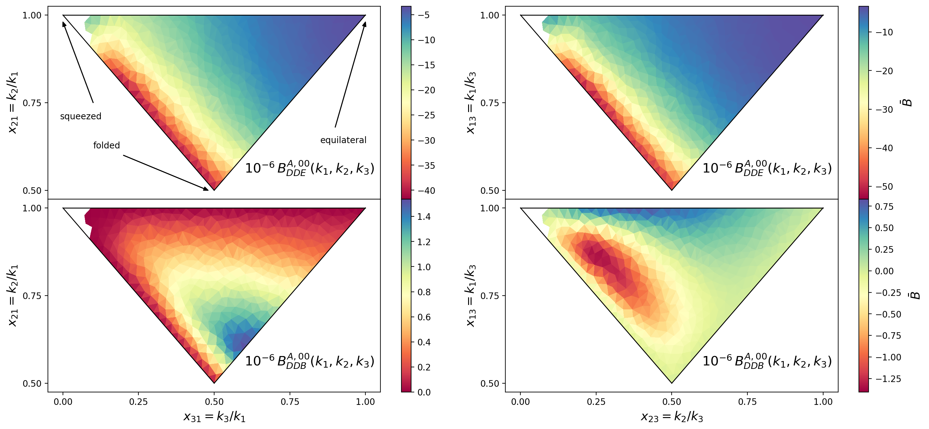
Figure 1: Signal as a function of triangle shape for intrinsic alignment bispectrum multipoles with one single tensor mode. We show two distinct orderings, namely $k_{1}\geq k_{2}\geq k_{3}$ (left panel) and $k_{3}\geq k_{1}\geq k_{2}$ (right panel). The top (bottom) row shows the parity-even (odd) bispectrum.

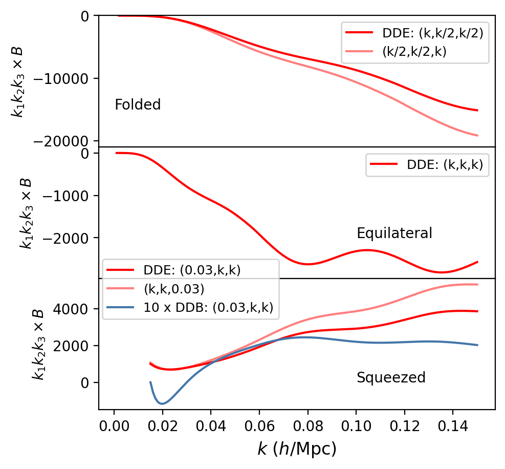
Figure 2: Signal as a function of triangle scale for the first nonzero intrinsic alignment bispectrum multipoles with one tensor mode, i.e. $(\ell_{1},\ell_{2})=(0,0)$. We show folded, equilateral and squeezed configurations.

Based on this, we define the ALMs of the bispectrum of shape fields with respect to the associated Legendre polynomials in this paper. Specifically, when one fixes $\hat{\mathbf{d}}=\hat{\mathbf{n}}$ then Eq. (3.4) reduces to Eq. (53). Thus, given that the ALMs are perhaps a more realistic proxy for what a (separable) LPP bispectrum estimator could measure when applied to a galaxy survey, we are motivated to examine the difference between OLMs and ALMs (see 82, for related work). However, we caution that we still treat the simulation box in the flat-sky approximation (i.e. the distant-observer or GPP limit) whereas a more realistic comparison would involve creating lightcones, applying a survey mask and explicitly incorporating wide-angle geometry. This is beyond the scope of our work.

3.5 Intrinsic Alignment Bispectra Visualized

Since we are only interested in the SNR of tensor bispectra, we will omit $B_{DDD}$ and only focus on deterministic parts $B^{\text{det,tree}}$ in the remainder of this paper. By the results of Section 3, we can ignore spectra with more than one B-mode. We thus no longer consider $B_{DDD},B_{DBB},B_{EBB}$ and $B_{BBB}$ and six combinations out of the 10 in Eq. (33) remain. To gain some intuition for the IA bispectrum signal, we present plots for the lowest order nonzero multipoles for all six combinations. This is $(\ell_{1},\ell_{2})=(0,0),(0,2),(2,2)$ for bispectra with one, two or three tensor fields. We can either use a triangle plot as in (86) to visualize the dependence on triangle shape, or fix the geometry of a triangle and plot the signal as a function of scale. For the former, we restrict ourselves to triangle configurations that satisfy $k_{l}\geq k_{m}\geq k_{n}$ and average the bispectrum over the largest triangle side, while keeping the ratios $x_{ml}=k_{m}/k_{l}$ and $x_{nl}=k_{n}/k_{l}$ fixed. For instance, assuming an ordering $k_{1}\geq k_{2}\geq k_{3}$, we have

$$\bar{B}_{XYZ}^{T,\ell_{1},\ell_{2}}(x_{21},x_{31})\equiv\int_{k_{\rm min}}^{k_{\rm max}}\mathrm{d}k\,\frac{B_{XYZ}^{T,\ell_{1},\ell_{2}}(k,\,x_{21}\,k,\,x_{31}\,k)}{k_{\rm max}-k_{\rm min}}\,,$$ (62)

and we average over $k_{1}$ values between $k_{\rm min}=0.01\,h\,\mathrm{Mpc}^{-1}$ and $k_{\rm max}=0.15\,h\,\mathrm{Mpc}^{-1}$. For bispectra involving multiple different fields, one cannot assume without loss of generality that the wavenumbers are ordered as such. In the following we therefore show different cases, focusing on $k_{1}\geq k_{2}\geq k_{3}$ and $k_{1}\geq k_{3}\geq k_{2}$ or $k_{3}\geq k_{1}\geq k_{2}$, and only the ALMs for the sake of brevity. The fiducial values of bias parameters used to generate these plots are identical to those for the ‘DESI LRG - like’ forecasting setup from Section 4.

When plotting the signal as a function of scale for a fixed triangle shape, we show equilateral, squeezed and collinear configurations, unless they evaluate to zero. For example, parity-odd bispectra evaluate to zero for collinear configurations, as reflections are equivalent to rotations for collinear triangles.

With this in mind, Figures 1,2 display the signal of the two single-tensor bispectra $B^{00}_{DDE}$ and $B^{00}_{DDB}$. We observe that $B^{00}_{DDB}$ is relatively suppressed compared to $B^{00}_{DDE}$, even though they are naïvely of the same order in perturbation theory. This was also observed in (57); note that in their notation the $s_{ij}$ and $t_{ij}$ terms in the bias expansion dominate the $B_{DDE}$ signal, but these contributions only project onto E-modes. Figures 3 and 4 show the bispectra with two tensor fields and finally Figures 5 and 6, those with three tensor fields.

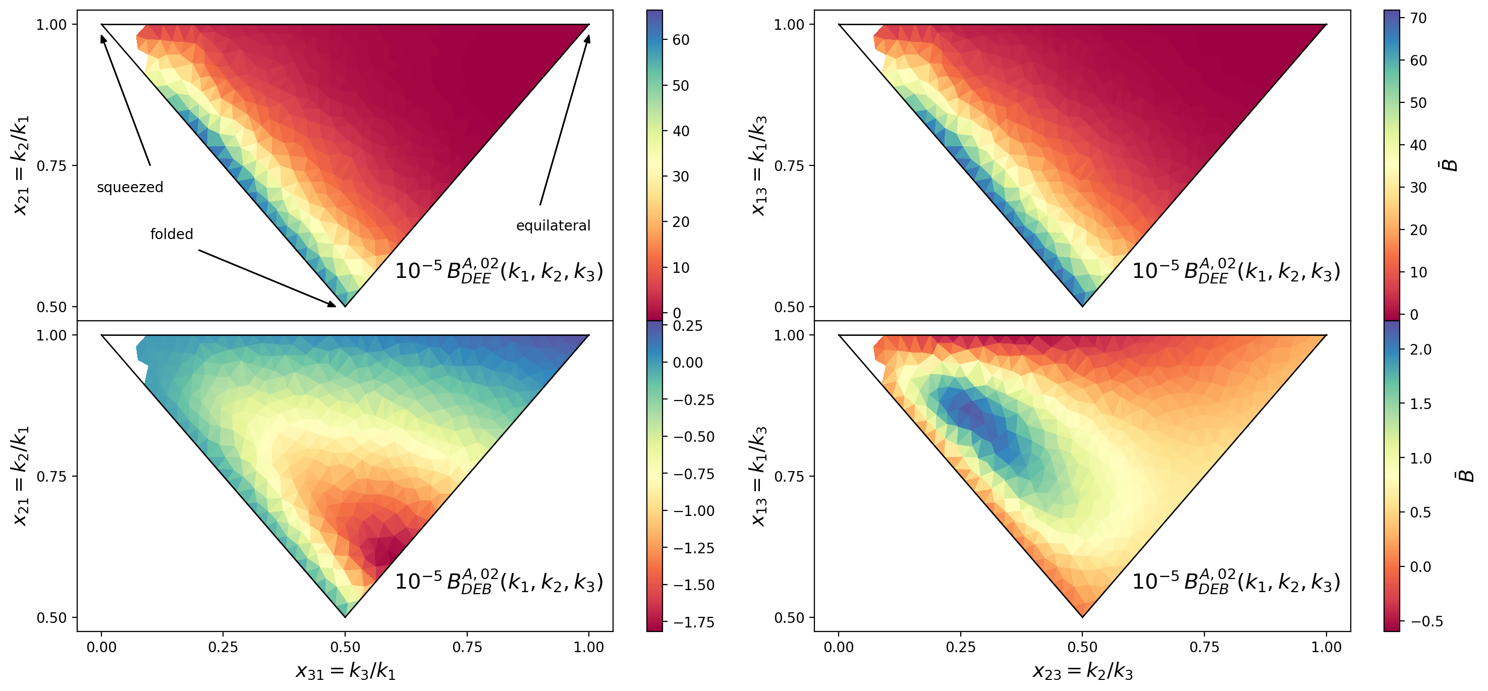
Figure 3: Signal as a function of triangle shape for intrinsic alignment bispectrum multipoles with two tensor modes. We show two distinct orderings, namely $k_{1}\geq k_{2}\geq k_{3}$ (left panel) and $k_{3}\geq k_{1}\geq k_{2}$ (right panel). The top (bottom) row shows the parity-even (odd) bispectrum.

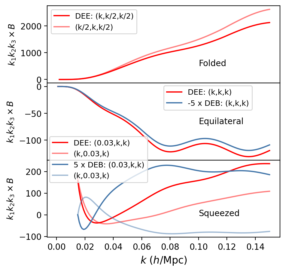
Figure 4: Signal as a function of triangle scale for the first nonzero intrinsic alignment bispectrum multipoles with two tensor modes, i.e. $(\ell_{1},\ell_{2})=(0,2)$. We show folded, equilateral and squeezed configurations.

Note that for $B_{DDB}^{00}$ and $B_{EEB}^{22}$ the signal is antisymmetric in its first two arguments, since swapping the first two sides of the triangle can be achieved by a reflection. Thus, the equilateral configurations evaluate to zero, whereas this is not the case for $B_{DEB}^{02}$. In all cases that involve only the density and $E$-mode fields, the shape dependence of the bispectrum is very similar to that of the auto density bispectrum $B_{DDD}$ (see e.g., 86) with an increase in amplitude from equilateral towards collinear triangle configurations (lower left side of the plotted triangular region). For bispectra that also contain a $B$-mode field, the shape dependence is more complex, displaying maxima (or minima) for triangle configurations different from all of the limiting cases. As mentioned above, this is because the bispectrum vanishes for folded and equilateral configurations. As we will see in Section 5, all spectra with more than one tensor are difficult to detect. As was the case for single-tensor bispectra, replacing an E-mode with a B-mode results in a suppression of the signal.

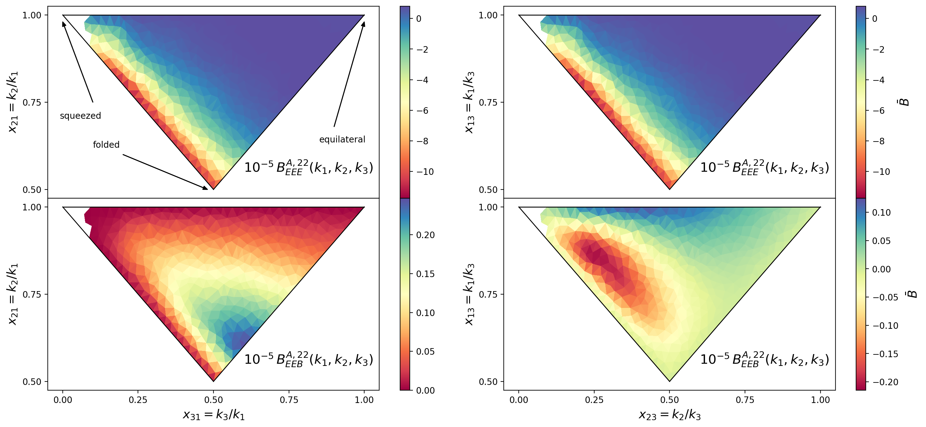
Figure 5: Signal as a function of triangle shape for intrinsic alignment bispectrum multipoles with three tensor modes. We show two distinct orderings, namely $k_{1}\geq k_{2}\geq k_{3}$ (left panel) and $k_{3}\geq k_{1}\geq k_{2}$ (right panel). The top (bottom) row shows the parity-even (odd) bispectrum.

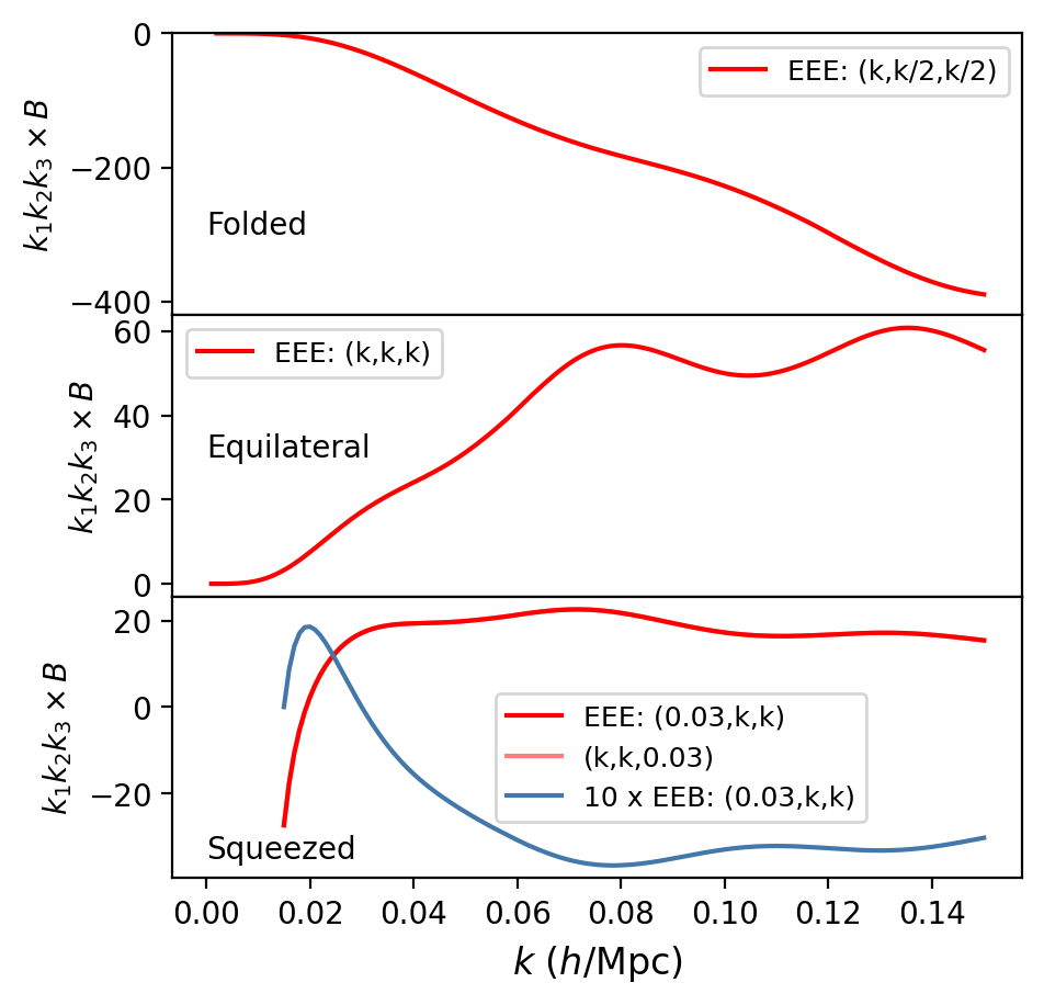
Figure 6: Signal as a function of triangle scale for the first nonzero intrinsic alignment bispectrum multipoles with three tensor modes, i.e. $(\ell_{1},\ell_{2})=(2,2)$. We show folded, equilateral and squeezed configurations.

4 Forecasting Setup

We are interested in the detectability of the anisotropic large-scale bispectrum of intrinsic alignments. For simplicity, we thus only focus on the SNR of the bispectrum multipoles and defer a joint analysis involving the power spectrum or sensitivity to any specific parameters to future work. The SNR is schematically given by

$$(S/N)^{2}=\sum_{L,L^{\prime},\{k_{i}\}}B^{L}(\{k_{i}\})C_{LL^{\prime},ij}^{-1}B^{L^{\prime}}(\{k_{j}\})$$ (63)

where $L=\ell_{1}\ell_{2}$ and $L^{\prime}=\ell_{1}^{\prime}\ell_{2}^{\prime}$ are generic multipole indices, $\{k_{i}\}$ denotes a triangle bin, $C_{LL^{\prime},ij}$ is the covariance and we suppress the fields $XYZ,X^{\prime}Y^{\prime}Z^{\prime}$ to avoid clutter. We consider wavenumbers $k_{i}$ from 15 linearly spaced bins of width $\Delta k=0.01\,h$/Mpc and we choose the lower edge of the first bin to be $k_{\text{min}}=\Delta k/2$, so that bin centers are integer multiples of $\Delta k$. Our setup thus includes collinear triangle bins, but not open triangle bins (i.e. where the bin centers do not form a closed triangle). The most challenging part of the forecast consists of computing the covariance matrix and its inverse, which we discuss next.

4.1 Covariance

We now turn to the calculation of the analytical Gaussian covariance of our multipole estimators. Since our analysis is restricted to large scales, this is a reasonable approach. We will show explicitly that the Gaussian approximation works well on the scales we consider here (78), which is in line with findings of (76). Another potential avenue for cross-checking the validity of the analytic Gaussian covariance would be via injecting intrinsic alignment into N-body simulations (e.g., as in 89).

As per the approach in (63), we will proceed to calculate the Gaussian covariance by plugging in the NLA model (46) predictions (including shape noise $c^{\text{g}}$) for the power spectra (see Appendix E). They are repeated below for convenience :

$$P_{EE}(k,\mu) =\frac{1}{4}(b_{1}^{\text{g}})^{2}(1-\mu^{2})^{2}P_{\text{NL}}(k)+c^{\text{g}};$$ (64)

$$P_{DE}(k,\mu) =\frac{1}{2}b_{1}^{\text{s}}b_{1}^{\text{g}}(1-\mu^{2})P_{\text{NL}}(k);$$

$$P_{BB}(k,\mu) =c^{\text{g}}.$$

For the galaxy power spectrum we also use a linear bias model:

$$P_{DD}(k)=(b_{1}^{\text{s}})^{2}P_{\text{NL}}(k)+c^{\text{s}}.$$ (65)

Here, $b_{1}^{\text{s}}$ is the familiar linear galaxy bias parameter and we take $c^{\text{s}}=1/\bar{n}$ where $\bar{n}$ is the number density of objects in the sample. Furthermore, $P_{\text{NL}}(k)$ is the nonlinear matter power spectrum, which we calculate using the CCL wrapper for HaloFit (90). To a good approximation, $c^{\text{g}}$ is just the typical ellipticity of the galaxy sample, i.e. $c^{\text{g}}=\sigma_{\gamma}^{2}/\bar{n}$ (63; 60). The linear alignment parameter $b_{1}^{\text{g}}$ can be expressed in terms of the more commonly used $A_{\text{IA}}$ via (63)

$$b_{1}^{\text{g}}=-2A_{\text{IA}}C_{1}\rho_{\text{cr}}\Omega_{m,0}/D(z),$$ (66)

where $D(z)$ is the linear growth factor and $C_{1}\rho_{\text{cr}}=0.0134$ (91; 46). It is understood that $b_{1}^{\text{g}}$ and $A_{\text{IA}}$ may also be redshift dependent. It was shown in related work (92) that this approximation works fairly well on large scales for the power spectrum covariance. If desired, the bispectrum-bispectrum and power spectrum-trispectrum terms could be included in the bispectrum covariance by using perturbation theory (93; 77; 94).

In the following, we always keep the ordering of the tracers (i.e. $XYZ$) fixed. This does not lose any generality, cf. Eq. (15). Because the tracers under consideration need not be the same ($X,Y,Z$ can be any of $D,E,B$), the multipoles $B_{XYZ}^{T,\ell_{1}\ell_{2}}(k_{1},k_{2},k_{3})$ are in general not symmetric with respect to their arguments, even when $\ell_{1}=\ell_{2}=0$. This needs to be taken into account when computing the covariance matrix associated with the bispectrum data vector. We cannot immediately impose an ordering on the triangle bins such as $k_{1}\geq k_{2}\geq k_{3}$, as one would typically do for galaxy clustering – this would in principle result in a loss of information (unless one then also considers all permutations of fields $XYZ$, which yields equivalence to our approach).

The result of the covariance calculation for an arbitrary cross-correlation of different multipoles, different tracers and different triangle bins can be found in Eq. (124). In particular, we can infer from this expression that two bispectra evaluated in isomorphic triangles (e.g. $(k_{1},k_{2},k_{3})$ and $(k_{2},k_{3},k_{1})$) are not identical, but they have a nontrivial cross correlation. This makes the inversion of even the Gaussian covariance matrix more difficult than for the clustering bispectrum (we elaborate on this below). To circumvent this issue, we can also consider symmetrized observables $\widetilde{B}$ which sum over all isomorphic triangle configurations. Explicitly,

$$\widetilde{B}_{XYZ}^{T,\ell_{1}\ell_{2}}(k_{1},k_{2},k_{3})=\frac{1}{6}\sum_{\sigma\in S_{3}}B^{T,\ell_{1}\ell_{2}}_{XYZ}(k_{\sigma(1)},k_{\sigma(2)},k_{\sigma(3)}).$$ (67)

For the symmetrized observables, we can by construction assume that $k_{1}\geq k_{2}\geq k_{3}$. Note that depending on $X,Y$ and $Z$ some terms in this average may be identical. The covariance of $\widetilde{B}$ is diagonal in $k$-space. However, the symmetrized estimate is essentially a form of data compression (it cannot be inverted) and thus in general lowers the SNR, as mentioned above. Quantifying the difference in SNR between $\widetilde{B}$ and $B$ is one of the objectives of this Section.

As a leading example, consider the covariance matrix of $B^{00}_{DDE}(k_{1},k_{2},k_{3}).$ This multipole is symmetric in its first two arguments and so we must impose $k_{1}\geq k_{2}$ to avoid overcounting. It consists of three parts, namely $C^{\text{gen}}$ for general triangles (i.e. with unequal sides), $C^{\text{isos}}$ for isosceles triangles and $C^{\text{equi}}$ for equilateral ones. Each of these has to be inverted separately. Indeed these types of triangles are uncorrelated, and the full covariance takes the following block diagonal form:

$$C=\begin{pmatrix}C^{\text{gen}}&0&0&0\\ 0&C^{\text{isos},1}&0&0\\ 0&0&C^{\text{isos},2}&0\\ 0&0&0&C^{\text{equi}}\end{pmatrix}.$$ (68)

We consider $C^{\text{gen}}$ first. Since the multipole is symmetric in the first two arguments, we must assume $k_{1}>k_{2}$ to avoid overcounting. Denoting wavenumber bins with integers for simplicity, we have that e.g. bin $(4,3,2)$ is covariant with bin $(4,2,3)$ and bin $(3,2,4)$, but we need not consider the other three permutations, because they do not satisfy $k_{1}>k_{2}$. Accordingly, $C^{\text{gen}}$ takes a 3 by 3 block form. For isosceles triangles, there are two distinct cases: in the first block, the equal sides are the longest (i.e. $(3,3,2),(3,2,3)$ since both should still satisfy $k_{1}\geq k_{2}$), or in the second block the equal sides are the shortest, for example $(2,2,3),(3,2,2)$. This makes $C^{\text{isos},i}$ a $2\times 2$ block matrix for $i=1,2$. We thus have

$$C^{\text{gen}}=\begin{pmatrix}C_{11}&C_{12}&C_{13}\\ C_{12}^{T}&C_{22}&C_{23}\\ C_{13}^{T}&C_{23}^{T}&C_{33}\end{pmatrix};\quad C^{\text{isos},i}=\begin{pmatrix}C_{11}^{i}&C_{12}^{i}\\ C^{i,T}_{12}&C_{22}^{i}\end{pmatrix};$$ (69)

where each of the $C_{ab},C_{ab}^{i}$ is diagonal. Finally, $C^{\text{equi}}$ is already diagonal and its inversion is trivial.

If we consider more multipoles (be it different $\ell_{1},\ell_{2}$ or different $X,Y,Z$) which are also symmetric in their first two arguments, then the only difference is that every entry in the above matrix is replaced by an $m\times m$ matrix, where $m$ is the number of multipoles considered. The process of inverting this matrix remains virtually unchanged, because the component matrices $C_{ij}$ from Eq. (69) are themselves still block diagonal. If the bispectrum has no exchange symmetries, as is the case for e.g. $B_{DEB}^{00}$ or $B_{DDE}^{20}$, analytically inverting the covariance would still be possible but we do not consider this case here. Finally, note that in the Gaussian approximation, there is no cross-correlation between parity-even and parity-odd bispectra. This makes it particularly easy to combine e.g. $B_{DDE}$ and $B_{DDB}$ if desired.

4.2 Analysis Choices

We need to estimate the values of the EFT parameters that enter the bispectrum predictions. For this, in our baseline analysis we will employ so-called Lagrangian co-evolution relations (63; 95), which assume that initially, a linear bias relation holds for the tracer in question and non-linear bias arises only through non-linear advection, such that we only need to specify the values of the linear alignment bias $b_{1}^{\text{g}}$ and the linear galaxy bias $b_{1}^{\text{s}}$. In modelling the signal, we set all of the stochastic parameters to zero so that $B^{\text{stoch,tree}}=0$. We neglect redshift uncertainties throughout, i.e. we require a spectroscopic sample in order to resolve the three-dimensional positions of the galaxies needed to construct the multipoles. We do not incorporate redshift-space distortions, but note that our multipole expansions and corresponding estimators are applicable also when they are included. We employ the Gaussian covariance from the previous subsection throughout.

Our default setup consists of a sample of luminous red galaxies (LRGs) from the Dark Energy Spectroscopic Instrument (DESI) (2) where we assume to have imaging from the Legacy Survey of Space and Time (LSST) (96). Given the sky coverage $f_{\text{sky}}$ and the redshift range of the survey, we can compute the total (comoving) survey volume as

$$V_{\text{survey}}=\frac{4}{3}\pi f_{\text{sky}}(\chi(z_{\text{max}})^{3}-\chi(z_{\text{min}})^{3})$$ (70)

By default, we use $A_{\text{IA}}=4$ from (14) and a volume-limited sample for $0.4<z<0.8$ with number density $\bar{n}=5\times 10^{-4}(h/\text{Mpc})^{3}$ (97). We evaluate the theory at a mean redshift of $z_{*}=0.6$. For the sky coverage we assume an area of $\sim 4,000$ square degrees ($f_{\text{sky}}=0.1$). This yields a total of $\sim 1.3$ million LRGs. The linear galaxy bias is estimated to be roughly $1.5/D(z_{*})\approx 2.05$(98). We use a fiducial maximum wavenumber of $k_{\rm{max}}=0.14\,h$/Mpc. The RMS shape dispersion is $\sigma_{\gamma}=0.18$ (per component).

We expect the highest SNR to come from $B_{DDE}^{00}$ (both for the OLMs and the ALMs), which is nonzero even if all the higher-order shape biases vanish (c.f. Table 2). Therefore, in the case of $B_{DDE}^{00}$ specifically, we also assess the difference between using a symmetrized estimator $\widetilde{B}$ as in Eq. (67) and using the full estimator which does not symmetrize over any of the wavevector arguments.

The expressions for the OLMs in general need to be integrated numerically; this is due to the presence of factors of $1-\mu_{i}^{2}$ in the denominator of Eq. (61). By contrast, the expressions for the ALMs and the covariance matrix from Eq. (124) are simple polynomials in $\cos\theta_{1},\sin\theta_{1}$ and $\cos\xi,\sin\xi$; they can be integrated analytically using the identities given in Appendix C.

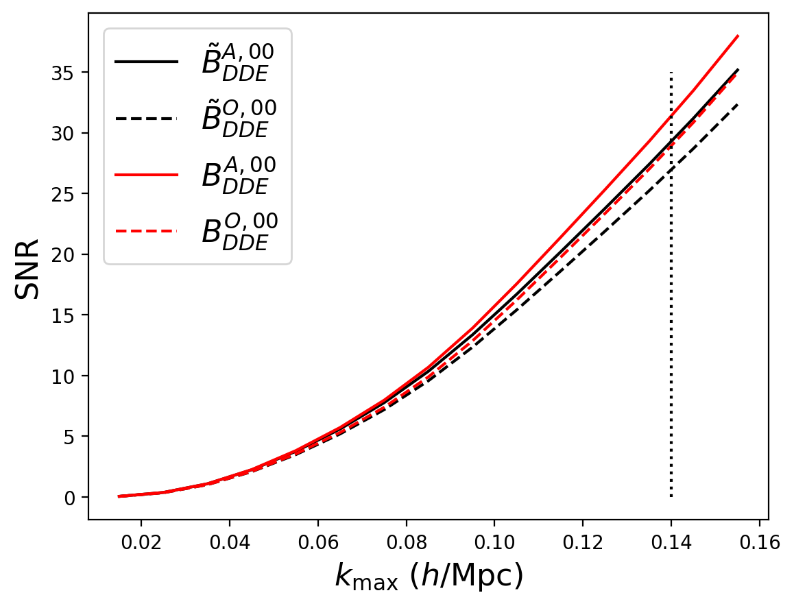
Figure 7: Cumulative signal-to-noise ratio as a function of maximum wavenumber for the lowest order associated and ordinary multipoles of $B_{DDE}$. Solid curves are ALMs, which always exceed the SNR of the OLMs (dashed curves). Red curves are unsymmetrized, which always exceed the SNR in the symmetrized case (black).

5 Results

We first assess the detectability of $B_{DDE}^{00}$. The SNR is highest if we do not compress the data vector by symmetrizing. Furthermore, we are interested in the difference between the use of OLMs and ALMs. The SNR for each of these four cases as a function of scale cut is plotted in Figure 7. The OLM expansion of the bispectra should strictly speaking contain the same amount of information as the ALM expansion. However, in practice the convergence of either series may differ when considering only a finite number of multipole moments (82). We see in this case that the SNR in the OLMs is consistently lower than that of the ALMs. Moreover, while the SNR in the unsymmetrized data vector is higher, the difference is small ($<10\%$). At $k_{\text{max}}=0.14\,h/$Mpc, indicated by the dashed vertical line, we obtain a promising SNR of $\approx 25-30$ in all cases.

Motivated by these results, we also examine the SNR in symmetrized higher-order multipoles of $B_{DDE}$, specifically $(\ell_{1},\ell_{2})=(1,1)$ and $(\ell_{1},\ell_{2})=(2,0)$. The result is shown in Figure 8. We predict significant detections for both these multipoles, at SNR $\approx 15$ at the fiducial scale cut for the ALMs. Again, the ALMs outperform the OLMs, with large differences for fixed $(\ell_{1},\ell_{2})$. However, the difference in the SNR obtained when combining these three multipoles (black lines) is very small. For completeness, we also display in Table 1 the SNR values for several specific triangle configurations. Interestingly, while for $(\ell_{1},\ell_{2})=(0,0)$ and $(2,0)$ the SNR peaks in the collinear configurations (third and fourth rows), it is the squeezed limit that contains the most SNR for $(\ell_{1},\ell_{2})=(1,1)$.

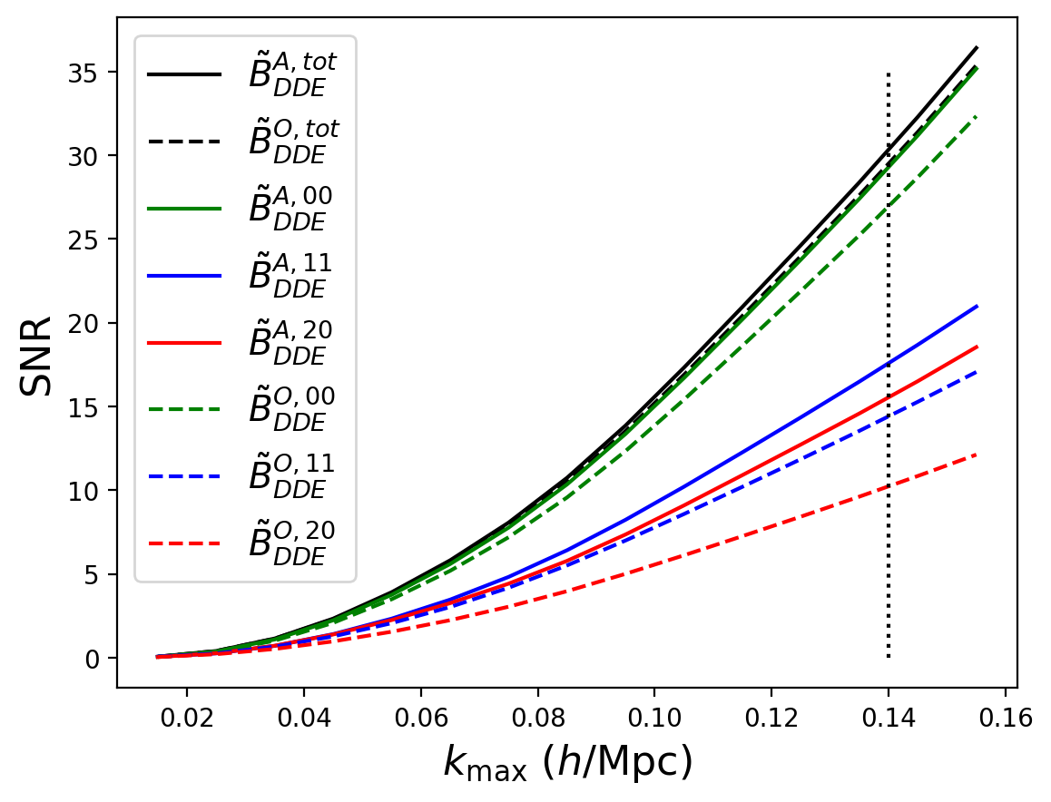
Figure 8: Cumulative signal-to-noise ratio as a function of maximum wavenumber for several symmetrized associated and ordinary multipoles of $B_{DDE}$. Solid (dashed) lines represent ALMs (OLMs) and black lines represent the SNR in the sum of the three multipoles.

Bin $(h/\text{Mpc})$ / $(\ell_{1},\ell_{2})$	$(0,0)$	$(1,1)$	$(2,0)$
$(0.05,0.05,0.05)$	0.29	0.34	0.22
$(0.10,0.10,0.10)$	0.33	0.39	0.26
$(0.15,0.10,0.05)$	3.22	0.51	2.43
$(0.14,0.07,0.07)$	2.60	0.40	1.96
$(0.15,0.15,0.10)$	0.69	0.73	0.41
$(0.15,0.15,0.03)$	1.07	0.92	0.37

Table 1: The SNR in specific triangle bins for different ALMs of $\tilde{B}_{DDE}$.

Next, we examine two multipoles of $B_{DDB}$, namely $(\ell_{1},\ell_{2})=(0,0)$ and $(\ell_{1},\ell_{2})=(1,1)$ in Figure 9. Here we find an important difference to that of $B_{DDE}^{00}$: after imposing $k_{1}\geq k_{2}$, the (Gaussian) covariance is already diagonal in $k$-space, by virtue of the fact that $P_{GB}(\mathbf{k})=0$ (one can easily check this using Eq. (124)). Thus, we do not symmetrize these multipoles (this symmetrization would also lead to zero signal since these bispectra are antisymmetric in their first two arguments). We see that the SNR of these bispectra is significantly suppressed compared to the parity-even case of $B_{DDE}$, consistent with the findings of Section 3. However, in this case the OLM expansion seems to outperform the ALM expansion. Still, the overall detection significance is more modest at SNR $\approx 5\,(2)$ for $(\ell_{1},\ell_{2})=(0,0)$ resp. $(\ell_{1},\ell_{2})=(1,1)$.

For the spectra with more than one tensor field, obtaining a detection is more challenging with our fiducial setup. Figure 10 displays the SNR for the lowest order multipoles of bispectra with two or three shape fields as a function of the scale cut $k_{\text{max}}$. Only $B_{DEE}$ seems detectable, at moderate significance at best (SNR $\approx 5$). The reason for this difference is similar to the situation for the alignment auto-power spectrum: since the linear alignment bias is very small $(b_{1}^{\text{g}}<0.1)$, the signal is noise-dominated essentially at all scales; $(b_{1}^{\text{g}})^{2}P_{L}(k)<\sigma_{\gamma}^{2}/\bar{n}$. This is even more exacerbated for the pure-tensor bispectra $B_{EEE}$ and $B_{EEB}$. Obtaining a sufficiently dense and aligned galaxy sample so as to detect these may be possible with samples that possess stronger intrinsic alignment or higher number density (see (99) for a potential way to increase the IA amplitude). In addition, it may be possible to detect these spectra in N-body simulations, in which case they provide additional consistency checks.

6 Discussion

We have shown in this work that (i) arbitrary bispectra of tensor fields can be modelled consistently within the framework of the effective field theory of intrinsic alignments; (ii) the resulting projected bispectra are either parity-even or parity-odd depending on the number of B-modes they contain; (iii) their estimation from spectroscopic galaxy samples via multipole decomposition and separable FFT-based algorithms is analogous to the existing literature on multipoles of the galaxy bispectrum in redshift space, both in the parity-even and the parity-odd case, and finally (iv) single-tensor parity-even bispectra are detectable on large scales with high SNR in Stage IV galaxy surveys, some of which are already operational.

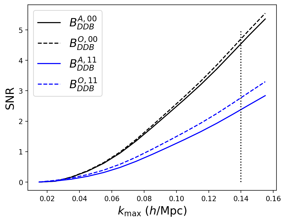
Figure 9: Cumulative signal-to-noise ratio as a function of maximum wavenumber for two associated and ordinary multipoles of $B_{DDB}$, namely $(\ell_{1},\ell_{2})=(0,0)$ (black) and $(\ell_{1},\ell_{2})=(1,1)$ (blue).

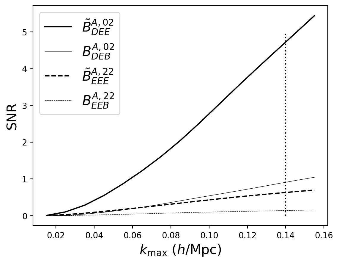
Figure 10: Cumulative signal-to-noise ratio as a function of maximum wavenumber for the lowest order associated multipoles of bispectra with more than one tensor field. Note that the odd bispectra are not symmetrized.

Our results can be extended or improved upon in various ways. Notably, it may be possible to increase the SNR by considering different ‘tensor tracers’ than LRG intrinsic alignment, such as the recently introduced ‘multiplet alignment’ from (100) or by employing different estimators that increase the IA amplitude (99). Second, the sky overlap with LSST is still not completely certain; in our fiducial setup the SNR is simply proportional to $\sqrt{f_{\text{sky}}}$ so that increasing it by a factor of $2$ would yield $\sim 40\%$ more SNR. Moreover, if one does not restrict to imaging from LSST but rather uses DESI Legacy imaging, shapes would be available for the entire DESI footprint (see (14) for a similar approach; the imaging quality requirements for intrinsic alignment measurements may not be as stringent as those for shear measurements). Moreover, there may also be significant overlap with the 4MOST galaxy survey in the southern hemisphere (101). These enhancements may also yield a positive detection of bispectra with more tensor fields. Crucially, we have also set all stochastic contributions to bispectra to zero and only considered the deterministic part of the bias expansion when computing the SNR. It may however still be possible to extract information from these contributions; we leave this for future work. It is also possible to extend the analysis presented here to smaller scales, which would appear to increase the SNR significantly. While the magnitude of the signal may not differ that much from the tree-level prediction beyond $k=0.14\,h$/Mpc, the covariance receives non-Gaussian contributions from higher order terms (77) and super-sample effects (60; 102) and is therefore considerably more uncertain. For the power spectrum of intrinsic alignments, (60) showed that this causes the cumulative SNR to eventually plateau.

Our findings could be extended to other three-point observables such as the three-point correlation function (3PCF) (103; 104) or aperture mass statistics (50). It would be valuable to quantify the increase in constraining power from retaining modes outside the plane of the sky ($\mu\neq 0$), for example by using wedges as done for the galaxy power spectrum (105). Moreover, statistics that are sensitive to specific triangle configurations may not extract all possible information from the alignment signal. For example, the equal-radius aperture mass statistic used in (49) is mostly sensitive to equilateral triangles (50), while the SNR for the bispectrum multipoles (see Table 1) does not peak there.

We anticipate that accurate knowledge of large-scale intrinsic alignment can help mitigate potential systematic selection effects that contaminate growth rate measurements via redshift-space distortions (25; 26). Moreover, the bispectrum is a useful probe in constraining primordial non-Gaussianity (106; 107). Consistently including the IA bispectrum in analyses constraining PNG would involve extending our modelling to include redshift-space distortions (108; 109). Furthermore, it would be interesting to explore the sensitivity of the IA bispectrum to any of the phenomena examined in the context of the IA power spectrum, examples of which include magnetic fields (17), modified gravity (22) or evolving dark energy (21). In addition, parity-odd bispectra (i.e. $B_{TTB}$) have proven useful in constraining graviton parity and Gaussianity using the Cosmic Microwave Background (CMB) temperature and polarization data (110) - it is in principle possible to also obtain bounds on primordial physics from LSS tracers (111; 112). Generally, IA can be used to place generic bounds on tensor perturbations via their impact on large-scale tidal fields (113; 19; 114).

With regards to weak gravitational lensing, the perturbative nature of our specific model may seem to restrict its applicability on small scales. However, (115) shows that perturbative models for IA (116) can still be used to extract the amplitude of matter fluctuations $S_{8}=\sigma_{8}\sqrt{\Omega_{m}/0.3}$ provided that one makes appropriate scale cuts. It would be very interesting to include three-point statistics in such an analysis. Moreover, the tree-level bispectrum model employed here correctly captures the angular and scale dependence of the anisotropic tensor bispectrum at least at leading order (78); it may be possible to formulate phenomenological extensions of it (in a similar vein to (49; 45)) that extend to smaller scales, in the same way that the NLA model extends the linear alignment model from (13) to smaller scales (46).

We have restricted ourselves to a calculation of only the SNR, rather than performing a full forecast for any specific parameter. In order to properly assess the sensitivity of the tensor bispectrum to any given parameter of interest in the Fisher matrix formalism (117), one requires knowledge of the corresponding derivative with respect to that parameter. It may be that the inclusion of the tensor bispectrum helps to break degeneracies between parameters, in which case the information gain exceeds what is expected from simply computing the SNR (relative to that of other statistics). We leave these considerations for future work. Lastly, in an upcoming follow-up paper (78) we will explicitly verify our theoretical modelling against N-body simulations, as done in (63).

Appendix A Explicit EFT expressions

Here we collect formulae for the tree-level tensor bispectrum in the EFT of IA. We first discuss the deterministic contributions and then stochastic terms, before summarizing the results. All expressions can be straightforwardly generalized to cases where not all shape tracers are the same, but we do not do this here to avoid clutter.

A.1 Deterministic Bispectrum Contributions

Here we provide explicit expressions for the deterministic part of the bispectrum $B^{\text{det,tree}}$. At tree-level, it contains only terms that involve four factors of the linear density contrast $\delta^{(1)}$. When the symmetric 2-tensor $S_{ij}$ is expanded in perturbation theory, it takes the form

$$S_{ij}(\mathbf{x})=\sum_{n=0}^{\infty}S_{ij}^{(n)}(\mathbf{x})$$ (71)

where the $n$-th order term in Fourier space is

$$S_{ij}^{(n)}(\mathbf{k})=\int\mathrm{d}^{3}\mathbf{p}_{1}\dots\mathrm{d}^{3}\mathbf{p}_{n}\,\mathcal{K}_{ij}^{(n)}(\mathbf{p}_{1},\dots\mathbf{p}_{n})\,\delta^{D}(\mathbf{k}-\mathbf{p}_{1n})\delta^{(1)}(\mathbf{p}_{1})\dots\delta^{(1)}(\mathbf{p}_{n}).$$ (72)

where $\mathbf{p}_{1n}=\mathbf{p}_{1}+\dots+\mathbf{p}_{n}$. Here the bias-dependent PT kernel $\mathcal{K}_{ij}^{(n)}$ splits into a trace and trace-free part:

$$\mathcal{K}_{ij}^{(n)}=\mathcal{K}_{ij}^{\text{s},(n)}+\mathcal{K}_{ij}^{\text{g},(n)}.$$ (73)

The total bispectrum of shape tracers at tree-level is then calculated to be

$$B_{ijklrs}^{\alpha\beta\gamma,\text{det,tree}}(\mathbf{k}_{1},\mathbf{k}_{2},\mathbf{k}_{3}) =2\,\mathcal{K}_{ij}^{\alpha,(1)}(\mathbf{k}_{1})\mathcal{K}_{kl}^{\beta,(1)}(\mathbf{k}_{2})\mathcal{K}_{rs}^{\gamma,(2)}(\mathbf{k}_{1},\mathbf{k}_{2})P_{L}(k_{1})P_{L}(k_{2})+\text{2 perm.};$$ (74)

where $\alpha,\beta,\gamma$ are either s or g and the overall factor of $2$ is a consequence of Wick’s theorem. The first order kernels are given by

$$\mathcal{K}_{ij}^{\text{s},(1)}(\mathbf{k}) =\frac{1}{3}\delta_{ij}b_{1}^{\text{s}};$$ (75)

$$\mathcal{K}_{ij}^{\text{g},(1)}(\mathbf{k}) =b_{1}^{\text{g}}\left(\frac{\mathbf{k}_{i}\mathbf{k}_{j}}{k^{2}}-\frac{1}{3}\delta_{ij}\right)=b_{1}^{\text{g}}\mathcal{D}_{ij}(\mathbf{k});$$

where in the second line we introduced the trace-free Fourier space operator $\mathcal{D}_{ij}(\mathbf{k})=\mathbf{k}_{i}\mathbf{k}_{j}/k^{2}-\frac{1}{3}\delta_{ij}$. Expressions for the second order kernels are

$$\mathcal{K}_{ij}^{\text{s},(2)}(\mathbf{k}_{1},\mathbf{k}_{2}) =\frac{1}{3}\delta_{ij}\bigg{[}b_{1}^{\text{s}}F_{2}(\mathbf{k}_{1},\mathbf{k}_{2})+b_{2,1}^{\text{s}}\bigg{(}\frac{(\mathbf{k}_{1}\cdot\mathbf{k}_{2})^{2}}{k_{1}^{2}k_{2}^{2}}\bigg{)}+b_{2,2}^{\text{s}}\bigg{]};$$ (76)

$$\mathcal{K}_{ij}^{\text{g},(2)}(\mathbf{k}_{1},\mathbf{k}_{2}) =\text{TF}\bigg{[}c_{1}^{\text{g}}\bigg{(}\frac{\mathbf{k}_{12,i}\mathbf{k}_{12,j}}{k_{12}^{2}}F_{2}(\mathbf{k}_{1},\mathbf{k}_{2})\bigg{)}+c_{2,1}^{\text{g}}\bigg{(}\frac{\mathbf{k}_{12,i}\mathbf{k}_{12,j}}{k_{12}^{2}}F_{2}(\mathbf{k}_{1},\mathbf{k}_{2})-\frac{1}{2}\frac{\mathbf{k}_{1}\cdot\mathbf{k}_{2}}{k_{1}^{2}k_{2}^{2}}(\mathbf{k}_{1,i}\mathbf{k}_{1,j}+\mathbf{k}_{2,i}\mathbf{k}_{2,j})\bigg{)}$$

$$+c_{2,2}^{\text{g}}\bigg{(}\frac{1}{2}\frac{\mathbf{k}_{1}\cdot\mathbf{k}_{2}}{k_{1}^{2}k_{2}^{2}}(\mathbf{k}_{1,i}\mathbf{k}_{2,j}+\mathbf{k}_{2,i}\mathbf{k}_{1,j})\bigg{)}+c_{2,3}^{\text{g}}\bigg{(}\frac{\mathbf{k}_{1,i}\mathbf{k}_{1,j}}{2k_{1}^{2}}+\frac{\mathbf{k}_{2,i}\mathbf{k}_{2,j}}{2k_{2}^{2}}\bigg{)}\bigg{]};$$

where $\mathbf{k}_{12}=\mathbf{k}_{1}+\mathbf{k}_{2}$ and the $F_{2}$ kernel equals the standard SPT expression

$$F_{2}(\mathbf{k}_{1},\mathbf{k}_{2})=\frac{5}{7}+\frac{1}{2}\frac{\mathbf{k}_{1}\cdot\mathbf{k}_{2}}{k_{1}k_{2}}\bigg{(}\frac{k_{1}}{k_{2}}+\frac{k_{2}}{k_{1}}\bigg{)}+\frac{2}{7}\frac{(\mathbf{k}_{1}\cdot\mathbf{k}_{2})^{2}}{k_{1}^{2}k_{2}^{2}}.$$ (77)

Here and in our companion paper as well as (58; 63), we choose to work with a redefinition of bias coefficients which is given by

$$b_{1}^{\text{s}} =c_{1}^{\text{s}};\qquad b_{2,1}^{\text{s}}=c_{2,2}^{\text{s}}+\frac{2}{7}c_{2,1}^{\text{s}};\qquad b_{2,2}^{\text{s}}=c_{2,3}^{\text{s}}+\frac{5}{7}c_{2,1}^{\text{s}};$$ (78)

$$b_{1}^{\text{g}} =c_{1}^{\text{g}};\qquad b_{2,1}^{\text{g}}=c_{2,1}^{\text{g}}+c_{2,2}^{\text{g}}+c_{2,3}^{\text{g}};\qquad b_{2,2}^{\text{g}}=c_{2,3}^{\text{g}}+\frac{20}{7}c_{2,1}^{\text{g}};\qquad b_{2,3}^{\text{g}}=c_{2,3}^{\text{g}}.$$

The coefficients $c_{2,a}^{\text{s}}$ can be related to other familiar bases by using the relations in App. B of (62). In the notation of (64), the coefficients $c_{1}^{\{\text{s,g}\}},c_{2,a}^{\{\text{s,g}\}}(a=1,2,3)$ belong to trace and trace-free parts of the operators

$$\Pi^{[1]}_{ij},\Pi^{[2]}_{ij},(\Pi^{[1]})^{2}_{ij},\Pi^{[1]}_{ij}\text{Tr}(\Pi^{[1]}_{ij})$$ (79)

respectively - thus, there are only two independent bias coefficients for the trace part. By contrast, the trace-free part contains three free parameters. Importantly, it is insufficient to write an expansion for the total symmetric tensor field $S_{ij}$ and then equate the coefficients occurring in the trace and trace-free parts (58). This can ultimately be explained as a consequence of renormalization of the bare coefficients.

We will need the co-evolution relations for the second order parameters in terms of $b_{1}^{\text{s}}$ and $b_{1}^{\text{g}}$, which are derived under the assumption that the Lagrangian higher order bias parameters are zero. They read

$$b_{2,1}^{\text{g}}=(b_{1}^{\text{s}}-1)b_{1}^{\text{g}};\qquad b_{2,2}^{\text{g}}=(b_{1}^{\text{s}}-20/7)b_{1}^{\text{g}};\qquad b_{2,3}^{\text{g}}=b_{1}^{\text{s}}b_{1}^{\text{g}}.$$ (80)

We will also need the co-evolution relations for the scalar bias parameters, which read (62)

$$b_{2,1}^{\text{s}}=b_{K^{2}}=-\frac{2}{7}(b_{1}^{\text{s}}-1);\qquad b_{2,2}^{\text{s}}=b_{\delta^{2}}-\frac{1}{3}b_{K^{2}}=\frac{10}{21}(b_{1}^{\text{s}}-1).$$ (81)

This part of the bispectrum already appeared in (57), albeit in a less general setting. Our treatment also differs from theirs in terms of the stochastic contributions, which were not considered in their work. We describe these next.

A.2 Stochastic Contributions

We now discuss the stochastic contributions to the scalar and shape kernels. For the scalar part we have two terms contributing to the galaxy bias expansion (both of which are absent for dark matter). They are well known and read

$$\delta_{D}^{\text{stoch}}(\mathbf{x})\qquad\supset\qquad\epsilon(\mathbf{x})\text{ (first order) };\qquad\epsilon^{\delta}(\mathbf{x})\delta(\mathbf{x})\text{ (second order) }.$$ (82)

Moving on to the shape part, there are two new independent bias operators contributing to the tree-level bispectrum. They are

$$g_{ij}^{\text{stoch}}(\mathbf{x})\qquad\supset\qquad\epsilon_{ij}(\mathbf{x})\text{ (first order) };\qquad\epsilon_{ij}^{\delta}(\mathbf{x})\delta(\mathbf{x}),\quad\epsilon^{\Pi}(\mathbf{x})\text{TF}(\Pi^{[1]})_{ij}(\mathbf{x})\text{ (second order) }.$$ (83)

The relevant stochastic contractions we can form with these fields (that is, using at most one second order operator and omitting combinations that come with only one instance of $\delta(\mathbf{x}$) are

$$\langle\epsilon(\mathbf{k}_{1})\epsilon(\mathbf{k}_{2})\rangle^{\prime} =\alpha_{\text{ss}}^{11}+\mathcal{O}((k/k_{\text{NL}})^{2});$$ (84)

$$\langle\epsilon(\mathbf{k}_{1})\epsilon^{\delta}(\mathbf{k}_{2})\rangle^{\prime} =\alpha_{\text{ss}}^{1\delta}+\mathcal{O}((k/k_{\text{NL}})^{2});$$

$$\langle\epsilon(\mathbf{k}_{1})\epsilon_{ij}^{\delta}(\mathbf{k}_{2})\rangle^{\prime} =0+\mathcal{O}((k/k_{\text{NL}})^{2});$$

$$\langle\epsilon_{ij}(\mathbf{k}_{1})\epsilon(\mathbf{k}_{2})\rangle^{\prime} =0+\mathcal{O}((k/k_{\text{NL}})^{2});$$

$$\langle\epsilon_{ij}(\mathbf{k}_{1})\epsilon^{\Pi}(\mathbf{k}_{2})\rangle^{\prime} =0+\mathcal{O}((k/k_{\text{NL}})^{2});$$

$$\langle\epsilon_{ij}(\mathbf{k}_{1})\epsilon^{\delta}(\mathbf{k}_{2})\rangle^{\prime} =0+\mathcal{O}((k/k_{\text{NL}})^{2});$$

$$\langle\epsilon(\mathbf{k}_{1})\epsilon^{\Pi}(\mathbf{k}_{2})\rangle^{\prime} =\alpha_{\text{sg}}^{1\Pi}+\mathcal{O}((k/k_{\text{NL}})^{2});$$

$$\langle\epsilon_{ij}(\mathbf{k}_{1})\epsilon_{kl}(\mathbf{k}_{2})\rangle^{\prime} =\alpha_{\text{gg}}^{11}\Delta_{ij,kl}^{\text{TF}}+\mathcal{O}((k/k_{\text{NL}})^{2});$$

$$\langle\epsilon_{ij}(\mathbf{k}_{1})\epsilon^{\delta}_{kl}(\mathbf{k}_{2})\rangle^{\prime} =\alpha_{\text{gg}}^{1\delta}\Delta_{ij,kl}^{\text{TF}}+\mathcal{O}((k/k_{\text{NL}})^{2});$$

$$\langle\epsilon(\mathbf{k}_{1})\epsilon(\mathbf{k}_{2})\epsilon(\mathbf{k}_{3})\rangle^{\prime} =\alpha_{\text{sss}}^{111}+\mathcal{O}((k/k_{\text{NL}})^{2});$$

$$\langle\epsilon(\mathbf{k}_{1})\epsilon(\mathbf{k}_{2})\epsilon_{ij}(\mathbf{k}_{3})\rangle^{\prime} =0+\mathcal{O}((k/k_{\text{NL}})^{2});$$

$$\langle\epsilon(\mathbf{k}_{1})\epsilon_{ij}(\mathbf{k}_{2})\epsilon_{kl}(\mathbf{k}_{3})\rangle^{\prime} =\alpha_{\text{sgg}}^{111}\Delta_{ij,kl}^{\text{TF}}+\mathcal{O}((k/k_{\text{NL}})^{2});$$

$$\langle\epsilon_{ij}(\mathbf{k}_{1})\epsilon_{kl}(\mathbf{k}_{2})\epsilon_{rs}(\mathbf{k}_{3})\rangle^{\prime} =\alpha_{\text{ggg}}^{111}\Delta_{ij,kl,rs}^{\text{TF}}+\mathcal{O}((k/k_{\text{NL}})^{2}).$$

Here the $\alpha$ parameters are stochastic amplitudes, which we label according to the nature of the fields being correlated (scalar s or tensor g) and the specific stochastic operator label $1,\Pi,\delta$ for $\epsilon,\epsilon^{\delta},\epsilon^{\Pi}$ respectively. There are five in total for the tensor sector (i.e. where at least one tensor field is involved) and three for the pure scalar sector. The stochastic amplitude $\alpha_{\text{gg}}^{11}$ also occurred in (63) and is related to the shape-noise amplitude in the EE- and BB- power spectra $c^{\text{g}}$ from Eq. (64) through $2\alpha_{\text{gg}}^{11}=c^{\text{g}}$. The symbol $\Delta^{\text{TF}}$ is the total pair-symmetric, pair-traceless tensor: it is symmetric under exchange of pairs, and traceless symmetric in each pair. It is a uniquely defined expression in terms of the Kronecker delta (up to an irrelevant constant). The total the pair-symmetric, pair-traceless tensor with four indices is given by

$$\Delta^{\text{TF}}_{ij,kl}=\delta_{ik}\delta_{jl}+\delta_{il}\delta_{jk}-\frac{2}{3}\delta_{ij}\delta_{kl}.$$ (85)

The total pair-symmetric, pair-traceless tensor with six indices is given by (58)

$$\Delta_{ij,kl,rs}^{\text{TF}} =\frac{4}{3}\delta_{ij}\delta_{kl}\delta_{rs}+\frac{3}{4}\bigg{(}\delta_{ik}\delta_{jr}\delta_{ls}+\delta_{ik}\delta_{js}\delta_{lr}+\delta_{il}\delta_{jr}\delta_{ks}+\delta_{il}\delta_{js}\delta_{lr}+\delta_{ir}\delta_{jk}\delta_{ls}+\delta_{ir}\delta_{js}\delta_{kl}$$ (86)

$$+\delta_{is}\delta_{jk}\delta_{lr}+\delta_{is}\delta_{jr}\delta_{kl}\bigg{)}-\bigg{(}\delta_{ij}(\delta_{kr}\delta_{ls}+\delta_{ks}\delta_{lr})+\delta_{kl}(\delta_{ir}\delta_{js}+\delta_{is}\delta_{jr})+\delta_{rs}(\delta_{il}\delta_{jk}+\delta_{ik}\delta_{jl})\bigg{)}.$$

For scalar spectra we recover the familiar combinations

$$B^{\text{sss}}\supset\langle\epsilon(\mathbf{k}_{1})\epsilon(\mathbf{k}_{2})\epsilon(\mathbf{k}_{3})\rangle^{\prime} =\alpha_{\text{sss}}^{111}+\mathcal{O}((k/k_{\text{NL}})^{2});$$ (87)

$$B^{\text{sss}}\supset\langle(b_{1}^{\text{s}}\delta)(\mathbf{k}_{1})\epsilon(\mathbf{k}_{2})(\epsilon^{\delta}\delta)(\mathbf{k}_{3})\rangle^{\prime} =b_{1}^{\text{s}}\alpha_{\text{ss}}^{1\delta}P_{L}(k_{1})+\mathcal{O}((k/k_{\text{NL}})^{2});$$

where the second line should be symmetrized over $\mathbf{k}_{1},\mathbf{k}_{2}$ and $\mathbf{k}_{3}$. The relevant spectra containing tensor fields take the form

$$B_{ij}^{\text{ssg}} \supset\langle\epsilon(\mathbf{k}_{1})(b_{1}^{\text{s}}\delta)(\mathbf{k}_{2})(\epsilon^{\Pi}\text{TF}(\Pi^{[1]})_{kl})(\mathbf{k}_{3})\rangle^{\prime}=b_{1}^{\text{s}}\alpha_{\text{sg}}^{1\Pi}\mathcal{D}_{kl}(\mathbf{k}_{2})P_{L}(k_{2})+\mathcal{O}((k_{i}/k_{\text{NL}})^{2});$$ (88)

$$B_{ij}^{\text{ssg}} \supset\langle\epsilon(\mathbf{k}_{1})(\epsilon^{\delta}\delta)(\mathbf{k}_{2})(b_{1}^{\text{g}}\text{TF}(\Pi^{[1]})_{kl})(\mathbf{k}_{3})\rangle^{\prime}=b_{1}^{\text{g}}\alpha_{\text{ss}}^{1\delta}\mathcal{D}_{kl}(\mathbf{k}_{3})P_{L}(k_{3})+\mathcal{O}((k_{i}/k_{\text{NL}})^{2});$$

$$B_{ijkl}^{\text{sgg}} \supset\langle\epsilon(\mathbf{k}_{1})(b_{1}^{\text{g}}\text{TF}(\Pi^{[1]})_{ij})(\mathbf{k}_{2})(\epsilon^{\Pi}\text{TF}(\Pi^{[1]})_{kl})(\mathbf{k}_{3})\rangle^{\prime}=b_{1}^{\text{g}}\alpha_{\text{sg}}^{1\Pi}\mathcal{D}_{ij}(\mathbf{k}_{2})\mathcal{D}_{kl}(\mathbf{k}_{3})P_{L}(k_{2})+\mathcal{O}((k_{i}/k_{\text{NL}})^{2});$$

$$B_{ijkl}^{\text{sgg}} \supset\langle\epsilon(\mathbf{k}_{1})\epsilon_{ij}(\mathbf{k}_{2})\epsilon_{kl}(\mathbf{k}_{3})\rangle^{\prime}=\alpha_{\text{sgg}}^{111}\Delta_{ij,kl}^{\text{TF}}+\mathcal{O}((k_{i}/k_{\text{NL}})^{2});$$

$$B_{ijkl}^{\text{sgg}} \supset\langle(b_{1}^{\text{s}}\delta)(\mathbf{k}_{1})\epsilon_{ij}(\mathbf{k}_{2})(\epsilon_{kl}^{\delta}\delta)(\mathbf{k}_{3})\rangle^{\prime}=b_{1}^{\text{s}}\alpha_{\text{gg}}^{1\delta}\Delta_{ij,kl}^{\text{TF}}P_{L}(k_{1})+\mathcal{O}((k_{i}/k_{\text{NL}})^{2});$$

$$B_{ijklrs}^{\text{ggg}} \supset\langle(b_{1}^{\text{g}}\text{TF}(\Pi^{[1]})_{ij})(\mathbf{k}_{1})(\epsilon_{kl}^{\delta}\delta)(\mathbf{k}_{2})\epsilon_{rs}(\mathbf{k}_{3})\rangle^{\prime}=b_{1}^{\text{g}}\alpha_{\text{gg}}^{1\delta}\mathcal{D}_{ij}(\mathbf{k}_{1})\Delta_{kl,rs}^{\text{TF}}P_{L}(k_{1})+\mathcal{O}((k_{i}/k_{\text{NL}})^{2});$$

$$B_{ijklrs}^{\text{ggg}} \supset\langle\epsilon_{ij}(\mathbf{k}_{1})\epsilon_{kl}(\mathbf{k}_{2})\epsilon_{rs}(\mathbf{k}_{3})\rangle^{\prime}=\alpha_{\text{ggg}}^{111}\Delta_{ij,kl,rs}^{\text{TF}}+\mathcal{O}((k_{i}/k_{\text{NL}})^{2}).$$

Care must be taken to symmetrize the above expressions over the indices and wavevectors. In particular, for the first line, there is also a contribution to $B^{\text{ssg}}$ where $\mathbf{k}_{2}$ is replaced with $\mathbf{k}_{1}$. Furthermore, lines 2 and 5 should be multiplied by a factor of 2 to obtain the total contribution and on line 3 there is a contribution with $\mathbf{k}_{2}$ and $\mathbf{k}_{3}$ exchanged. The sixth line should be summed over all six permutations of $\mathbf{k}_{1},\mathbf{k}_{2}$ and $\mathbf{k}_{3}$. One may also observe that $\alpha_{\text{ss}}^{11}$ and $\alpha_{\text{gg}}^{11}$ do not contribute to tree-level bispectra. Instead, they only occur in two-point statistics at leading order.

The $\mathcal{O}((k_{i}/k_{\text{NL}})^{2})$ terms indicate scale-dependent corrections to the constant amplitudes $\alpha$ as well as $k$-dependent tensorial structures such as

$$\alpha_{\text{ggg}}^{\Pi}\left(k_{\text{NL}}^{-2}(\mathbf{k}_{1,i}\mathbf{k}_{1,j}-\frac{1}{3}\delta_{ij}k_{1}^{2})\Delta_{kl,rs}+2\text{ perm.}\right);$$ (89)

(for the last line of Eq. (88) specifically) and many more, which necessarily start at higher order since $\hat{\mathbf{k}}_{i}$ is not allowed by locality in space.

Thus, the total tensorial bispectrum (before projecting shapes into E- and B-fields) contains a total of 13 free parameters at tree-level (excluding higher-derivative corrections), namely

$$\underbrace{b_{1}^{\{\text{s,g}\}},b_{2,1}^{\{\text{s,g}\}},b_{2,2}^{\{\text{s,g}\}},b_{2,3}^{\text{g}}}_{\text{bias expansion (7)}},\quad\underbrace{\alpha_{\text{ss}}^{1\delta},\alpha_{\text{sg}}^{1\Pi},\alpha_{\text{gg}}^{1\delta},\alpha_{\text{sss}}^{111},\alpha_{\text{sgg}}^{111},\alpha_{\text{ggg}}^{111}}_{\text{stochasticity (6)}}.$$ (90)

It actually turns out that we do not need to consider $\alpha_{\text{ggg}}^{111}$ in the analysis of projected shapes, as we show below. It is easy to verify that

$$\mathbf{M}^{X}_{ij}(\hat{\mathbf{k}}_{1})\mathbf{M}^{Y}_{kl}(\hat{\mathbf{k}}_{2})\Delta^{\text{TF}}_{ij,kl} =2\text{ Tr}(\mathbf{M}^{X}(\hat{\mathbf{k}}_{1})\mathbf{M}^{Y}(\hat{\mathbf{k}}_{2}));$$ (91)

$$\mathbf{M}^{X}_{ij}(\hat{\mathbf{k}}_{1})\mathbf{M}^{Y}_{kl}(\hat{\mathbf{k}}_{2})\mathbf{M}^{Z}_{rs}(\hat{\mathbf{k}}_{3})\Delta^{\text{TF}}_{ij,kl,rs} =3\text{ Tr}(\mathbf{M}^{X}(\hat{\mathbf{k}}_{1})\mathbf{M}^{Y}(\hat{\mathbf{k}}_{2})\mathbf{M}^{Z}(\hat{\mathbf{k}}_{3}))+3\text{ Tr}(\mathbf{M}^{Y}(\hat{\mathbf{k}}_{2})\mathbf{M}^{X}(\hat{\mathbf{k}}_{1})\mathbf{M}^{Z}(\hat{\mathbf{k}}_{3})).$$

By the cyclicity of the trace, these two expressions are fully symmetric in $X,Y,Z$. The expression on the first line can be evaluated for the different combinations of E- and B-fields as

$$2\text{ Tr}(\mathbf{M}^{E}(\hat{\mathbf{k}}_{2})\mathbf{M}^{E}(\hat{\mathbf{k}}_{3})) =\cos 2(\phi_{2}-\phi_{3});$$ (92)

$$2\text{ Tr}(\mathbf{M}^{E}(\hat{\mathbf{k}}_{2})\mathbf{M}^{B}(\hat{\mathbf{k}}_{3})) =\sin 2(\phi_{2}-\phi_{3});$$

$$2\text{ Tr}(\mathbf{M}^{B}(\hat{\mathbf{k}}_{2})\mathbf{M}^{B}(\hat{\mathbf{k}}_{3})) =\cos 2(\phi_{2}-\phi_{3}).$$

As expected, they only depend on the differences between azimuthal angles $\phi_{i}$. The expressions on the right-hand side can be expressed in terms of $\mu_{1}$ and $\xi$. Specifically, we have

$$\cos 2\phi_{2} =\frac{\mu_{12}^{2}(1-\mu_{1}^{2})+2\mu_{1}\mu_{12}\sqrt{(1-\mu_{1}^{2})(1-\mu_{12}^{2})}\cos\xi-(1-\mu_{12}^{2})(\sin^{2}\xi-\mu_{1}^{2}\cos^{2}\xi)}{1-\mu_{2}^{2}};$$ (93)

$$\sin 2\phi_{2} =\frac{2\sqrt{1-\mu_{12}^{2}}\big{(}\mu_{12}\sqrt{1-\mu_{1}^{2}}+\mu_{1}\sqrt{1-\mu_{12}^{2}}\cos\xi\big{)}\sin\xi}{1-\mu_{2}^{2}};$$

$$\cos 2\phi_{3} =\frac{(1-\mu_{1}^{2})(k_{1}+k_{2}\mu_{12})^{2}+k_{2}\big{(}2\mu_{1}(k_{1}+2k_{2}\mu_{12})\sqrt{(1-\mu_{1}^{2})(1-\mu_{12}^{2})}\cos\xi-k_{2}(1-\mu_{12}^{2})(\sin^{2}\xi-\mu_{1}^{2}\cos^{2}\xi)\big{)}}{k_{3}^{2}(1-\mu_{3}^{2})};$$

$$\sin 2\phi_{3} =\frac{2k_{2}\big{(}(k_{1}+k_{2}\mu_{12})\sqrt{(1-\mu_{1}^{2})(1-\mu_{12}^{2})}+k_{2}\mu_{1}(1-\mu_{12}^{2})\cos\xi\big{)}\sin\xi}{k_{3}^{2}(1-\mu_{3}^{2})};$$

where

$$\mu_{2} =\mu_{1}\mu_{12}-\sqrt{(1-\mu_{1}^{2})(1-\mu_{12}^{2})}\cos\xi;$$ (94)

$$\mu_{3} =-\frac{\mu_{1}(k_{1}+k_{2}\mu_{12})+k_{2}\sqrt{(1-\mu_{1}^{2})(1-\mu_{12}^{2})}\cos\xi}{k_{3}};$$

all assuming without loss of generality that $\phi_{1}=0$. Remarkably, the expression in the second line of Eq. (91) always vanishes for every combination of E- and B-fields. Hence, the three-point function of the stochastic shape noise $\epsilon_{ij}(\mathbf{x})$ does not contribute to spectra of projected quantities. Nevertheless, this contribution, corresponding to $\alpha_{\text{ggg}}^{111}$, is present at the 3D level.

A.3 Total Bispectrum

Here we summarize broadly the structure of the total expressions for the tree-level bispectrum. As mentioned in Section 3, all contributions to spectra with a single B-mode are odd in $\xi$, that is, $B_{DDB},B_{DEB}$ and $B_{EEB}$. This is because changing $\xi$ to $-\xi$ amounts to reflecting the triangle in the $\mathbf{k}_{1}-\hat{\mathbf{n}}$ plane, and these spectra are odd under such reflections (which, again, does not mean that these spectra are zero, because the triangle does not get mapped onto itself). Moreover, since

$$\mathbf{M}_{ij}^{B}(\hat{\mathbf{k}})\mathcal{K}_{ij}^{\text{g},(1)}(\mathbf{k})=b_{1}^{\text{g}}\,\mathbf{M}_{ij}^{B}(\hat{\mathbf{k}})\mathcal{D}_{ij}(\mathbf{k})\delta(\mathbf{k})=0,$$ (95)

the B-mode starts at second order, and all contributions to $B_{BBB}$ vanish at tree level. We hence do not include it anymore. There are however stochastic contributions to $B_{DBB}$ and $B_{EBB}$. It is instructive to tabulate all the dependencies of the bispectra on the list of parameters that occur at tree level. Here we use the letter $D$ to indicate a generic scalar tracer, e.g. galaxy number counts. Note that $\alpha_{\text{ss}}^{11},\alpha_{\text{gg}}^{11}$ and $\alpha_{\text{ggg}}^{111}$ have been omitted; none of the bispectra depend on these parameters. Thus, the multipoles $B_{XYZ}$ with $X,Y,Z$ = $D,E,B$ depend on 12 free parameters in total (seven deterministic, five stochastic). The dependencies are indicated in Table 2 below.

$B$ / Bias

$b_{1}^{\text{s}}$

$b_{2,1}^{\text{s}}$

$b_{2,2}^{\text{s}}$

$b_{1}^{\text{g}}$

$b_{2,1}^{\text{g}}$

$b_{2,2}^{\text{g}}$

$b_{2,3}^{\text{g}}$

$\alpha_{\text{ss}}^{1\delta}$

$\alpha_{\text{sg}}^{1\Pi}$

$\alpha_{\text{gg}}^{1\delta}$

$\alpha_{\text{sss}}^{111}$

$\alpha_{\text{sgg}}^{111}$

$B_{GGG}$

✓

✓

✓

$\boldsymbol{\times}$

$\boldsymbol{\times}$

$\boldsymbol{\times}$

$\boldsymbol{\times}$

✓

$\boldsymbol{\times}$

$\boldsymbol{\times}$

✓

$\boldsymbol{\times}$

$B_{GGE}$

✓

✓

✓

✓

✓

✓

✓

✓

✓

$\boldsymbol{\times}$

$\boldsymbol{\times}$

$\boldsymbol{\times}$

$B_{GGB}$

✓

$\boldsymbol{\times}$

$\boldsymbol{\times}$

$\boldsymbol{\times}$

✓

✓

✓

$\boldsymbol{\times}$

✓

$\boldsymbol{\times}$

$\boldsymbol{\times}$

$\boldsymbol{\times}$

$B_{GEE}$

✓

✓

✓

✓

✓

✓

✓

$\boldsymbol{\times}$

✓

✓

$\boldsymbol{\times}$

✓

$B_{GBB}$

$\boldsymbol{\times}$

$\boldsymbol{\times}$

$\boldsymbol{\times}$

$\boldsymbol{\times}$

$\boldsymbol{\times}$

$\boldsymbol{\times}$

$\boldsymbol{\times}$

$\boldsymbol{\times}$

$\boldsymbol{\times}$

✓

$\boldsymbol{\times}$

✓

$B_{GEB}$

✓

$\boldsymbol{\times}$

$\boldsymbol{\times}$

✓

✓

✓

✓

$\boldsymbol{\times}$

$\boldsymbol{\times}$

✓

$\boldsymbol{\times}$

✓

$B_{EEE}$

$\boldsymbol{\times}$

$\boldsymbol{\times}$

$\boldsymbol{\times}$

✓

✓

✓

✓

$\boldsymbol{\times}$

$\boldsymbol{\times}$

✓

$\boldsymbol{\times}$

$\boldsymbol{\times}$

$B_{EEB}$

$\boldsymbol{\times}$

$\boldsymbol{\times}$

$\boldsymbol{\times}$

✓

✓

✓

✓

$\boldsymbol{\times}$

$\boldsymbol{\times}$

✓

$\boldsymbol{\times}$

$\boldsymbol{\times}$

$B_{EBB}$

$\boldsymbol{\times}$

$\boldsymbol{\times}$

$\boldsymbol{\times}$

$\boldsymbol{\times}$

$\boldsymbol{\times}$

$\boldsymbol{\times}$

$\boldsymbol{\times}$

$\boldsymbol{\times}$

$\boldsymbol{\times}$

✓

$\boldsymbol{\times}$

$\boldsymbol{\times}$

Table 2: Parameter dependence of tensorial bispectra.

There can be additional ‘accidental’ degeneracies when only considering specific multipoles at tree level; for example in the case of $B_{DDB}$ one can easily check that all OLMs and ALMs of $B_{DDB}$ depend only on the combinations $c_{2,1}^{\text{g}}+c_{2,2}^{\text{g}}=b_{2,1}^{\text{g}}-b_{2,3}^{\text{g}}$ and $c_{2,3}^{\text{g}}=b_{2,3}^{\text{g}}$, and furthermore the lowest order ALM $(\ell_{1}=\ell_{2}=0,m_{Z}=2)$, namely

$$B_{DDB}^{A,00}(k_{1},k_{2},k_{3})\propto\frac{1}{4\pi}\int\mathrm{d}\mu_{1}\mathrm{d}\xi\,(1-\mu_{3}^{2})\mathbf{M}_{ij}^{B}(\hat{\mathbf{k}}_{3})\mathcal{K}_{ij}^{\text{g},(2)}(\mathbf{k}_{1},\mathbf{k}_{2})$$ (96)

depends only on $c_{2,1}^{\text{g}}+c_{2,2}^{\text{g}}+c_{2,3}^{\text{g}}=b_{2,1}^{\text{g}}$. These degeneracies would be broken either by considering higher multipole moments, or (in the case of the second order operator biases) by adding loop corrections (31). If we considered the tensor power spectrum too (at one loop), there would be four additional parameters, namely $\alpha_{\text{ss}}^{11},\alpha_{\text{gg}}^{11}$ and two non-local counterterms $b_{R}^{\{\text{s,g}\}}$ proportional to $k^{2}P_{L}(k)$. If we only consider bispectra with at most one tensor field, the stochastic parameters $\alpha_{\text{gg}}^{1\delta}$ and $\alpha_{\text{sgg}}^{111}$ drop out and the bispectra depend on 10 free parameters (seven from the bias expansion and three stochastic amplitudes, as mentioned at the end of Section 2).

Appendix B Angular Bases for the Bispectrum

Instead of integrating the three-dimensional bispectra against spherical harmonics, we can also integrate against Legendre polynomials of different cosines, i.e. $\mathcal{L}_{\ell}(\mu_{2})$ (31). These can be written in terms of the spherical harmonics basis by noting that

$$\mu_{2}=\mu_{1}\mu_{12}+Y_{1}^{1}(\mu_{1},\xi)-Y_{1}^{-1}(\mu_{1},\xi)=\mu_{12}Y_{10}(\mu_{1},\xi)-\sqrt{2}Y_{11}(\mu_{1},\xi).$$ (97)

Thus, any Legendre polynomial in $\mu_{2}$ is ultimately a linear combination of real spherical harmonics of cosine type, since spherical harmonics of cosine type remain of cosine type when taking products. Conversely, every real spherical harmonic of cosine type can be written as a linear combination of Legendre polynomials of $\mu_{1}$ and $\mu_{2}$, for which we provide an argument below. As such, bispectra that are even under parity transformations can be completely described in terms of either basis. The Legendre basis is certainly more convenient, as separable estimators in terms of Legendre polynomials are easy to implement. The proof of the equivalence is a straightforward induction argument over $\ell$ for every $m$. Recall the definition of the associated Legendre polynomial

$$\mathcal{L}_{\ell}^{m}(\mu_{1})=(-1)^{m}(1-\mu_{1}^{2})^{m/2}\bigg{(}\frac{\mathrm{d}}{\mathrm{d}\mu_{1}}\bigg{)}^{m}\mathcal{L}_{\ell}(\mu_{1})$$ (98)

for $m\geq 0$, and the relation

$$\mathcal{L}_{\ell}^{-m}(\mu_{1})=(-1)^{m}\frac{(\ell-m)!}{(\ell+m)!}\mathcal{L}_{\ell}^{m}(\mu_{1})$$ (99)

extends the definition to $m<0$. Note that when $m$ is fixed, $\mathcal{L}_{\ell}^{m}$ is only nonzero for $\ell\geq|m|$. To see how a spherical harmonic of cosine type can be written as a linear combination of polynomials of $\mu_{1}$ and $\mu_{2}$, consider $m>0$ to be fixed. We can use the explicit expression

$$Y_{\ell m}(\mu_{1},\xi)=(-1)^{m}\sqrt{\frac{2\ell+1}{2\pi}\frac{(\ell-m)!}{(\ell+m)!}}\mathcal{L}_{\ell}^{m}(\mu_{1})\cos{(m\,\xi)}=(-1)^{m}c_{\ell m}\mathcal{L}_{\ell}^{m}(\mu_{1})\cos{(m\,\xi)}$$ (100)

as well as a recursion relation for associated Legendre polynomials of the form

$$(\ell-m+1)\mathcal{L}_{\ell+1}^{m}(\mu_{1})=(2\ell+1)\mu_{1}\mathcal{L}_{\ell}^{m}(\mu_{1})-(\ell+m)\mathcal{L}_{\ell-1}^{m}(\mu_{1})$$ (101)

(which is also valid for $\ell=m$ and $\ell=m-1$) to see that for some nonzero constants $a_{\ell m},a^{\prime}_{\ell m},a^{\prime\prime}_{\ell m}$,

$$a_{\ell m}Y_{\ell+1\,m}(\mu_{1},\xi)=a^{\prime}_{\ell m}\mu_{1}Y_{\ell m}(\mu_{1},\xi)+a^{\prime\prime}_{\ell m}Y_{\ell-1\,m}(\mu_{1},\xi).$$ (102)

Thus, if the claim holds for all $\ell^{\prime}\leq\ell$, then it also holds for $\ell^{\prime}=\ell+1$. It therefore suffices to show that the claim holds for $\ell=m$. In that case, we can in fact write

$$Y_{mm}(\mu_{1},\xi)=c_{mm}(2m-1)!!\bigg{(}\sqrt{1-\mu_{1}^{2}}\bigg{)}^{m}\cos{(m\,\xi)}.$$ (103)

But $\cos{(m\,\xi)}$ is just a polynomial in $\cos\xi$ of degree $m$ (more precisely, $\cos{(m\,\xi)}=T_{m}(\cos\xi)$ where $T_{m}$ is a Chebyshev polynomial of the first kind). Moreover, it is even or odd depending on the parity of $m$. Thus, if we write

$$\cos{(m\,\xi)}=w_{m}(\cos\xi)^{m}+w_{m-2}(\cos\xi)^{m-2}+\dots,$$ (104)

then we immediately get

$$Y_{mm}(\mu_{1},\xi)=c_{mm}(2m-1)!!\bigg{[}w_{m}\bigg{(}\sqrt{1-\mu_{1}^{2}}\cos\xi\bigg{)}^{m}+(1-\mu_{1}^{2})w_{m-2}\bigg{(}\sqrt{1-\mu_{1}^{2}}\cos\xi\bigg{)}^{m-2}+\dots\bigg{]}.$$ (105)

However, we also know that

$$\sqrt{1-\mu_{1}^{2}}\cos\xi=\frac{\mu_{2}-\mu_{12}\mu_{1}}{\sqrt{1-\mu_{12}^{2}}}$$ (106)

so that the statement is proved for $Y_{mm}$. This argument also shows that using all of the real spherical harmonics of cosine type up to a given $\ell$ is equivalent to using all combinations of Legendre polynomials up to a total degree $\ell$: if the $Y_{\ell m}$ on the RHS of Eq. (102) are at most of total degree $\ell$ in $\mu_{1}$ and $\mu_{2}$, then the LHS is at most of degree $\ell+1$. In summary, the set of multipoles $B^{\ell m}$ from Eq. (43) is equivalent to the set of OLMs $B^{O,\ell_{1}\ell_{2}}$ from Eq. (47) for parity-even bispectra. There are $(\ell+1)(\ell+2)/2$ multipoles to be formed up to total degree $\ell$. For example, for $\ell_{\text{max}}=2$ there are six multipoles: one monopole, two dipoles with $(\ell_{1},\ell_{2})=(0,1),(1,0)$ and three quadrupoles with $(\ell_{1},\ell_{2})=(2,0),(1,1),(0,2)$ (see (31) for an equivalent enumeration of the three quadrupoles).

Additionally, if we consider the parity-odd bispectra expanded in the sine type basis, we can write for $m<0$ (and for slightly different $c_{\ell m}$ than the ones above)

$$Y_{\ell m}(\mu_{1},\xi)=(-1)^{m}\sqrt{\frac{2\ell+1}{2\pi}\frac{(\ell-|m|)!}{(\ell+|m|)!}}\mathcal{L}_{\ell}^{|m|}(\mu_{1})\sin{(|m|\,\xi)}=(-1)^{m}c_{\ell m}\mathcal{L}_{\ell}^{|m|}(\mu_{1})\sin{(|m|\,\xi)}.$$ (107)

The first parity-odd multipole $B^{\ell m}$ appearing is $B^{1\,-1}$ since

$$\hat{\mathbf{n}}\cdot(\hat{\mathbf{q}}_{1}\times\hat{\mathbf{q}}_{2})=\sqrt{(1-\mu_{1}^{2})(1-\mu_{12}^{2})}\sin\xi=-\sqrt{(1-\mu_{12}^{2})}\sqrt{\frac{4\pi}{3}}Y_{1\,-1}(\mu_{1},\xi).$$ (108)

We can show that all the other real spherical harmonic multipoles $B^{\ell m}$ with $m<0$ can be constructed by taking linear combinations of Legendre polynomials of $\mu_{1}$ and $\mu_{2}$ multiplied by $Y_{1\,-1}$. The proof is analogous, so we start by taking $m<0$ to be fixed. After using the same recursion relation for the associated Legendre polynomials again, we conclude that we need to prove the claim for $\ell=|m|$. We now express $\sin{(|m|\,\xi)}$ as $\sin\xi$ multiplied by a polynomial in $\cos\xi$ of lesser degree (note $|m|\geq 1$; and this polynomial is the Chebyshev polynomial of the second kind $U_{|m|-1}(x)$):

$$\sin{(|m|\,\xi)}=\sin\xi\bigg{(}w_{|m|-1}(\cos\xi)^{|m|-1}+w_{|m|-3}(\cos\xi)^{|m|-3}+\dots\bigg{)}$$ (109)

Thus,

$$Y_{|m|m}(\mu_{1},\xi) =c_{|m||m|}(2|m|-1)!!\bigg{(}\sqrt{1-\mu_{1}^{2}}\bigg{)}^{|m|}\sin{(|m|\,\xi)}$$ (110)

$$=c_{|m||m|}(2|m|-1)!!\bigg{(}\sqrt{1-\mu_{1}^{2}}\sin\xi\bigg{)}$$

$$\times\bigg{[}w_{|m|-1}\bigg{(}\sqrt{1-\mu_{1}^{2}}\cos\xi\bigg{)}^{|m|-1}+(1-\mu_{1}^{2})w_{|m|-3}\bigg{(}\sqrt{1-\mu_{1}^{2}}\cos\xi\bigg{)}^{|m|-3}+\dots\bigg{]}$$

where we recognize $Y_{1\,-1}$ on the second line, and the expression involving Legendre polynomials on the third. Thus, considering all spherical harmonics of sine type up to a given $\ell$ is equivalent to considering all products of $Y_{1\,-1}$ with Legendre polynomials of total degree $\ell-1$, and there are $\ell(\ell+1)/2$ such combinations. Thus, the parity odd multipoles $B^{\ell m}$ from Eq. (44) are completely equivalent to the parity-odd OLMs $B^{O,\ell_{1}\ell_{2}}$ from Eq. (48).

While these arguments show that the above expansions are complete, it may still be that some multipoles are mathematically identical in case two of the sides are equal or some of the tracers are. We elaborate on this in Section 4.

Appendix C Symbolic Angular Integration

In our implementation, we found it practical where possible to rewrite all symbolic integrations necessary for the computation of the multipoles themselves and the covariance matrices in terms of the angular variables $\mu_{1}$ and $\xi$. Then, one can proceed by using

$$I_{n_{1},n_{2}}=\int_{-1}^{1}\mathrm{d}\mu_{1}\big{(}\sqrt{1-\mu_{1}^{2}}\big{)}^{n_{1}-1}\mu_{1}^{n_{2}}=\int_{0}^{\pi}\mathrm{d}\theta_{1}\sin^{n_{1}}\theta_{1}\cos^{n_{2}}\theta_{1}=(1+(-1)^{n_{2}})\frac{\Gamma(\frac{1+n_{1}}{2})\Gamma(\frac{1+n_{2}}{2})}{2\Gamma(\frac{2+n_{1}+n_{2}}{2})}.$$ (111)

so that

$$\frac{1}{4\pi}\int\mathrm{d}\mu_{1}\mathrm{d}\xi\,\bigg{(}\big{(}\sqrt{1-\mu_{1}^{2}}\big{)}^{n_{1}}\mu_{1}^{n_{2}}\sin^{m_{1}}\xi\cos^{m_{2}}\xi\bigg{)}=\frac{1}{4\pi}I_{n_{1}+1,n_{2}}I_{m_{1},m_{2}}(1+(-1)^{m_{1}}).$$ (112)

Appendix D Spectra with Parity-odd Fields

Some of our results regarding non-vanishing three-point statistics with an odd number of B-modes may appear to be at odds with current literature. For example, (72; 45) claim that such spectra should vanish based on symmetry arguments. However, as has already been noted in e.g. (57) and in our main text, in contrast to two-point statistics, performing a reflection in a plane containing the line of sight does not in general map a bispectrum triangle onto itself. Therefore, the relation that is inferred from parity symmetry reads (taking $B_{DDB}$ as an example)

$$B_{DDB}(\mathbf{k}_{1}^{\prime},\mathbf{k}_{2}^{\prime},\mathbf{k}_{3}^{\prime})=-B_{DDB}(\mathbf{k}_{1},\mathbf{k}_{2},\mathbf{k}_{3})$$ (113)

rather than $B_{DDB}(\mathbf{k}_{1},\mathbf{k}_{2},\mathbf{k}_{3})=-B_{DDB}(\mathbf{k}_{1},\mathbf{k}_{2},\mathbf{k}_{3})$ where the latter would imply that the bispectrum vanishes. By contrast, the power spectrum $P_{DB}(k,\mu)$ actually only depends on the magnitude of the wavevector and its angle with the line of sight $\mu$, both of which do not change under a reflection $\mathbf{P}$. Thus, we do have the implication

$$P_{DB}(\mathbf{k})=P_{DB}(\mathbf{k}^{\prime})=-P_{DB}(\mathbf{k})\implies P_{DB}(\mathbf{k})=0.$$ (114)

There is an additional caveat: even though odd three-dimensional bispectra do not vanish (but rather are odd under reflections), an angular average of such an odd function may vanish. For example, we saw that

$$B_{DDB}^{\ell m}(k_{1},k_{2},k_{3})=\frac{2\ell+1}{4\pi}\int\mathrm{d}\mu_{1}\mathrm{d}\xi\,B_{DDB}(k_{1},k_{2},k_{3},\mu,\xi)Y_{\ell m}(\mu,\xi)=0$$ (115)

for any positive $m$, because of the vanishing integral over $\xi$. It is beyond the scope of this work to write down explicit expressions for general line-of-sight-integrated bispectra and other three point statistics such as the aperture mass (49; 120; 121; 37). However, we remark that null measurements of ‘odd’ statistics such as $\langle M_{\text{ap}}^{2}(\theta)M_{\times}(\theta)\rangle$ need to be interpreted with caution when attempting to translate them to conclusions about the three-point statistic inside the integrand. An integral of an odd statistic may also vanish if the statistic is evaluated in a ‘symmetric’ configuration, such as a collinear or equilateral triangle (see the discussion in Section 5).

Appendix E Gaussian Covariance

Here we compute the Gaussian contribution to the bispectrum covariance. The binned estimator for the standard bispectrum multipoles is given by

$$\hat{B}^{T,\ell_{1}\ell_{2}}_{XYZ}(k_{1},k_{2},k_{3})=\frac{N_{\ell_{1}\ell_{2}}}{N_{\Delta}V}\sum_{\mathbf{q}_{i}\in\text{bin }i}\delta^{K}(\mathbf{q}_{123})\hat{X}(\mathbf{q}_{1})\hat{Y}(\mathbf{q}_{2})\hat{Z}(\mathbf{q}_{3})\mathcal{P}_{XYZ}^{T,\ell_{1}\ell_{2}}(\{\hat{\mathbf{q}}_{i}\}).$$ (116)

Hence, the sum runs over all the wavenumber triplets that fall within the specified bin and sum to zero. The normalization factor $N_{\Delta}$ equals the number of fundamental triangles present in the $(k_{1},k_{2},k_{3})$ bin. We do not order the bins. The quantity $\hat{X}$ refers to the measured field, i.e. it is evaluated on a discrete grid by means of FFTs.The Kronecker delta symbol $\delta^{K}$ equals unity when its argument is zero and zero otherwise. To compute the sum above in practice, we use the FFT-based estimator from (35). The measured fields can be related to the theory spectra via the relations

$$\langle\hat{X}(\mathbf{q}_{1})\hat{Y}(\mathbf{q}_{2})\rangle =V\delta^{K}(\mathbf{q}_{12})P_{XY}(\mathbf{q}_{1});$$ (117)

$$\langle\hat{X}(\mathbf{q}_{1})\hat{Y}(\mathbf{q}_{2})\hat{Z}(\mathbf{q}_{3})\rangle =V\delta^{K}(\mathbf{q}_{123})B_{XYZ}(\mathbf{q}_{1},\mathbf{q}_{2},\mathbf{q}_{3}).$$

As usual, one can ‘realize’ the ensemble average $\langle\cdot\rangle$ over initial conditions by generating a sufficient number of independent simulations. By using the second line of Eq. (117), we see that the ensemble average of the estimator equals

$$\langle\hat{B}^{T,\ell_{1}\ell_{2}}_{XYZ}(k_{1},k_{2},k_{3})\rangle =\frac{N_{\ell_{1}\ell_{2}}}{N_{\Delta}}\sum_{\mathbf{q}_{i}\in\text{bin }i}\delta^{K}(\mathbf{q}_{123})B_{XYZ}(\mathbf{q}_{1},\mathbf{q}_{2},\mathbf{q}_{3})\mathcal{P}_{XYZ}^{T,\ell_{1}\ell_{2}}(\{\hat{\mathbf{q}}_{i}\})$$ (118)

$$\approx\frac{N_{\ell_{1}\ell_{2}}}{V_{\Delta}}\int_{k_{1}}\mathrm{d}^{3}\mathbf{q}_{1}\int_{k_{2}}\mathrm{d}^{3}\mathbf{q}_{2}\int_{k_{3}}\mathrm{d}^{3}\mathbf{q}_{3}\,\delta^{D}(\mathbf{q}_{123})B_{XYZ}(\mathbf{q}_{1},\mathbf{q}_{2},\mathbf{q}_{3})\mathcal{P}_{XYZ}^{T,\ell_{1}\ell_{2}}(\{\hat{\mathbf{q}}_{i}\})$$

$$\approx\frac{N_{\ell_{1}\ell_{2}}}{4\pi}\int\mathrm{d}\mu_{1}\mathrm{d}\xi\,B_{XYZ}(k_{1},k_{2},k_{3},\mu_{1},\xi)\mathcal{P}_{XYZ}^{T,\ell_{1}\ell_{2}}(\mu_{1},\xi),$$

where in the second line we used the continuous approximation to make the replacement

$$\frac{1}{N_{\Delta}}\sum_{\mathbf{q}_{i}\in\text{bin }i}\delta^{K}(\mathbf{q}_{123})\approx\frac{1}{V_{\Delta}}\int_{k_{1}}\mathrm{d}^{3}\mathbf{q}_{1}\int_{k_{2}}\mathrm{d}^{3}\mathbf{q}_{2}\int_{k_{3}}\mathrm{d}^{3}\mathbf{q}_{3}\,\delta^{D}(\mathbf{q}_{123});$$ (119)

with $V_{\Delta}$ the volume of the integration region . In the third line we employed the thin-shell approximation so that the radial integrals over the bins become trivial and the angular average is a spherical integral, viz. for an arbitrary rotationally invariant integrand $U(\mathbf{q}_{1},\mathbf{q}_{2},\mathbf{q}_{3})$ (that is, an integrand only depends on the orientation of the triangle with respect to the line of sight) we assert that (122)

$$\frac{1}{V_{\Delta}}\int_{k_{1}}\mathrm{d}^{3}\mathbf{q}_{1} \int_{k_{2}}\mathrm{d}^{3}\mathbf{q}_{2}\int_{k_{3}}\mathrm{d}^{3}\mathbf{q}_{3}\,\delta^{D}(\mathbf{q}_{123})\,U(\mathbf{q}_{1},\mathbf{q}_{2},\mathbf{q}_{3})\approx\frac{1}{4\pi}\int\mathrm{d}\mu_{1}\mathrm{d}\xi\,U(k_{1},k_{2},k_{3},\mu_{1},\xi).$$ (120)

We can also use (cf. Eq. (49))

$$\hat{\mathbf{n}}\cdot(\hat{\mathbf{q}}_{1}\times\hat{\mathbf{q}}_{2})=\sqrt{(1-\mu_{1}^{2})(1-\mu_{12}^{2})}\sin\xi$$ (121)

to express an odd projector in terms of $\mu_{1}$ and $\xi$ in the bottom line of Eq. (118).

In a similar vein, the covariance can also be calculated: we can correlate two arbitrary instances of Eq. (116) and subtract the product of their means to get

$$\langle\hat{B} {}^{T,\ell_{1}\ell_{2}}_{XYZ}(k_{1},k_{2},k_{3})\hat{B}^{T,\ell_{1}^{\prime}\ell_{2}^{\prime}}_{X^{\prime}Y^{\prime}Z^{\prime}}(k_{1}^{\prime},k_{2}^{\prime},k_{3}^{\prime})\rangle-\langle\hat{B}^{T,\ell_{1}\ell_{2}}_{XYZ}(k_{1},k_{2},k_{3})\rangle\langle\hat{B}^{T,\ell_{1}^{\prime}\ell_{2}^{\prime}}_{X^{\prime}Y^{\prime}Z^{\prime}}(k_{1}^{\prime},k_{2}^{\prime},k_{3}^{\prime})\rangle$$ (122)

$$=\frac{N_{\ell_{1}\ell_{2}}N_{\ell_{1}^{\prime}\ell_{2}^{\prime}}}{N_{\Delta}N_{\Delta^{\prime}}V^{2}}\sum_{\mathbf{q}_{i}\in\text{bin }i}\sum_{\mathbf{q}_{j}^{\prime}\in\text{bin }j}\delta^{K}(\mathbf{q}_{123})\delta^{K}(\mathbf{q}^{\prime}_{123})\times\bigg{(}\langle\hat{X}(\mathbf{q}_{1})\hat{Y}(\mathbf{q}_{2})\hat{Z}(\mathbf{q}_{3})\hat{X^{\prime}}(\mathbf{q}^{\prime}_{1})\hat{Y^{\prime}}(\mathbf{q}^{\prime}_{2})\hat{Z^{\prime}}(\mathbf{q}^{\prime}_{3})\rangle$$

$$-\langle\hat{X}(\mathbf{q}_{1})\hat{Y}(\mathbf{q}_{2})\hat{Z}(\mathbf{q}_{3})\rangle\langle\hat{X^{\prime}}(\mathbf{q}^{\prime}_{1})\hat{Y^{\prime}}(\mathbf{q}^{\prime}_{2})\hat{Z^{\prime}}(\mathbf{q}^{\prime}_{3})\rangle\bigg{)}\bigg{(}\mathcal{P}_{XYZ}^{T,\ell_{1}\ell_{2}}(\{\hat{\mathbf{q}}_{i}\})\mathcal{P}_{X^{\prime}Y^{\prime}Z^{\prime}}^{T,\ell_{1}^{\prime}\ell_{2}^{\prime}}(\{\hat{\mathbf{q}}^{\prime}_{i}\})\bigg{)}.$$

To simplify this, we will need to take a number of steps. The first term on the last line is a six-point function, so that we can expand the term in parentheses as

$$V^{-3} \bigg{(}\langle\hat{X}(\mathbf{q}_{1})\hat{Y}(\mathbf{q}_{2})\hat{Z}(\mathbf{q}_{3})\hat{X^{\prime}}(\mathbf{q}^{\prime}_{1})\hat{Y^{\prime}}(\mathbf{q}^{\prime}_{2})\hat{Z^{\prime}}(\mathbf{q}^{\prime}_{3})\rangle-\langle\hat{X}(\mathbf{q}_{1})\hat{Y}(\mathbf{q}_{2})\hat{Z}(\mathbf{q}_{3})\rangle\langle\hat{X^{\prime}}(\mathbf{q}^{\prime}_{1})\hat{Y^{\prime}}(\mathbf{q}^{\prime}_{2})\hat{Z^{\prime}}(\mathbf{q}^{\prime}_{3})\rangle\bigg{)}$$ (123)

$$=P_{XX^{\prime}}(\mathbf{q}_{1})P_{YY^{\prime}}(\mathbf{q}_{2})P_{ZZ^{\prime}}(\mathbf{q}_{3})\delta^{K}(\mathbf{q}_{11^{\prime}})\delta^{K}(\mathbf{q}_{22^{\prime}})\delta^{K}(\mathbf{q}_{33^{\prime}})+P_{XX^{\prime}}(\mathbf{q}_{1})P_{YZ^{\prime}}(\mathbf{q}_{2})P_{ZY^{\prime}}(\mathbf{q}_{3})\delta^{K}(\mathbf{q}_{11^{\prime}})\delta^{K}(\mathbf{q}_{23^{\prime}})\delta^{K}(\mathbf{q}_{32^{\prime}})$$

$$+P_{XY^{\prime}}(\mathbf{q}_{1})P_{YX^{\prime}}(\mathbf{q}_{2})P_{ZZ^{\prime}}(\mathbf{q}_{3})\delta^{K}(\mathbf{q}_{12^{\prime}})\delta^{K}(\mathbf{q}_{21^{\prime}})\delta^{K}(\mathbf{q}_{33^{\prime}})+P_{XY^{\prime}}(\mathbf{q}_{1})P_{YZ^{\prime}}(\mathbf{q}_{2})P_{ZX^{\prime}}(\mathbf{q}_{3})\delta^{K}(\mathbf{q}_{12^{\prime}})\delta^{K}(\mathbf{q}_{23^{\prime}})\delta^{K}(\mathbf{q}_{31^{\prime}})$$

$$+P_{XZ^{\prime}}(\mathbf{q}_{1})P_{YY^{\prime}}(\mathbf{q}_{2})P_{ZX^{\prime}}(\mathbf{q}_{3})\delta^{K}(\mathbf{q}_{13^{\prime}})\delta^{K}(\mathbf{q}_{22^{\prime}})\delta^{K}(\mathbf{q}_{31^{\prime}})+P_{XZ^{\prime}}(\mathbf{q}_{1})P_{YX^{\prime}}(\mathbf{q}_{2})P_{ZY^{\prime}}(\mathbf{q}_{3})\delta^{K}(\mathbf{q}_{13}^{\prime})\delta^{K}(\mathbf{q}_{21^{\prime}})\delta^{K}(\mathbf{q}_{32^{\prime}})$$

$$=\sum_{\sigma\in S_{3}}P_{X\sigma(X^{\prime})}(\mathbf{q}_{1})P_{Y\sigma(Y^{\prime})}(\mathbf{q}_{2})P_{Z\sigma(Z^{\prime})}(\mathbf{q}_{3})\delta^{K}(\mathbf{q}_{1\sigma(1^{\prime})})\delta^{K}(\mathbf{q}_{2\sigma(2^{\prime})})\delta^{K}(\mathbf{q}_{3\sigma(3^{\prime})})$$

where we neglect higher-order corrections such as the bispectrum-bispectrum ($BB$), power spectrum-trispectrum ($PT$) and connected pentaspectrum ($T_{6}$) terms (123; 94) in the covariance, as well as the product of the estimator averages. These are at least eighth order in perturbations and therefore considered subdominant. In the bottom line, we have written the expression as a sum over six permutations $\sigma\in S_{3}$ which is understood to act on the ordered sets $\{X^{\prime},Y^{\prime},Z^{\prime}\}$ and $\{1,2,3\})$ simultaneously. We can conclude that the covariance vanishes if the triangles are not similar, i.e. if $(k_{1}^{\prime},k_{2}^{\prime},k_{3}^{\prime})$ is not a permutation of $(k_{1},k_{2},k_{3})$. After inserting the bottom line of Eq. (123) into Eq. (122) we can carry out the sums over the primed variables. For any permutation $\sigma$, the occurrence of $\delta^{K}(\mathbf{q}_{a\sigma(a^{\prime})})$ with $a=1,2$ or $3$ implies that we have to replace every occurrence of the primed vector $\mathbf{q}^{\prime}_{\sigma(a)}$ by $-\mathbf{q}_{a}$, or equivalently we should replace every $\mathbf{q}^{\prime}_{a}$ by $-\mathbf{q}_{\bar{\sigma}(a)}$ where $\bar{\sigma}$ is the inverse permutation of $\sigma$. This is especially relevant for the projector terms in Eq. (122), which contain unit vectors as their arguments. As such, these arguments need to be interchanged consistently. We obtain

$$\langle \hat{B}^{T,\ell_{1}\ell_{2}}_{XYZ}(k_{1},k_{2},k_{3})\hat{B}^{T,\ell_{1}^{\prime}\ell_{2}^{\prime}}_{X^{\prime}Y^{\prime}Z^{\prime}}(k_{1}^{\prime},k_{2}^{\prime},k_{3}^{\prime})\rangle-\langle\hat{B}^{T,\ell_{1}\ell_{2}}_{XYZ}(k_{1},k_{2},k_{3})\rangle\langle\hat{B}^{T,\ell_{1}^{\prime}\ell_{2}^{\prime}}_{X^{\prime}Y^{\prime}Z^{\prime}}(k_{1}^{\prime},k_{2}^{\prime},k_{3}^{\prime})\rangle$$ (124)

$$=\frac{N_{\ell_{1}\ell_{2}}N_{\ell_{1}^{\prime}\ell_{2}^{\prime}}V}{N_{\Delta}^{2}}\sum_{\mathbf{q}_{i}\in\text{bin }i}\delta^{K}(\mathbf{q}_{123})\times\bigg{(}\sum_{\sigma\in S_{3}}P_{X\sigma(X^{\prime})}(\mathbf{q}_{1})P_{Y\sigma(Y^{\prime})}(\mathbf{q}_{2})P_{Z\sigma(Z^{\prime})}(\mathbf{q}_{3})$$

$$\times\delta_{1\sigma(1)^{\prime}}\delta_{2\sigma(2)^{\prime}}\delta_{3\sigma(3)^{\prime}}\mathcal{P}_{XYZ}^{T,\ell_{1}\ell_{2}}(\{\hat{\mathbf{q}}_{i}\})\mathcal{P}_{X^{\prime}Y^{\prime}Z^{\prime}}^{T,\ell_{1}^{\prime}\ell_{2}^{\prime}}(\bar{\sigma}(\{-\hat{\mathbf{q}}_{i}\}))\bigg{)}$$

$$\approx\frac{N_{\ell_{1}\ell_{2}}N_{\ell_{1}^{\prime}\ell_{2}^{\prime}}V}{N_{\Delta}V_{\Delta}}\int_{k_{1}}\mathrm{d}^{3}\mathbf{q}_{1}\int_{k_{2}}\mathrm{d}^{3}\mathbf{q}_{2}\int_{k_{3}}\mathrm{d}^{3}\mathbf{q}_{3}\,\delta^{D}(\mathbf{q}_{123})\times\bigg{(}\sum_{\sigma\in S_{3}}P_{X\sigma(X^{\prime})}(\mathbf{q}_{1})P_{Y\sigma(Y^{\prime})}(\mathbf{q}_{2})P_{Z\sigma(Z^{\prime})}(\mathbf{q}_{3})$$

$$\times\delta_{1\sigma(1)^{\prime}}\delta_{2\sigma(2)^{\prime}}\delta_{3\sigma(3)^{\prime}}\mathcal{P}_{XYZ}^{T,\ell_{1}\ell_{2}}(\{\hat{\mathbf{q}}_{i}\})\mathcal{P}_{X^{\prime}Y^{\prime}Z^{\prime}}^{T,\ell_{1}^{\prime}\ell_{2}^{\prime}}(\bar{\sigma}(\{\hat{\mathbf{q}}_{i}\}))\bigg{)}$$

$$\approx\frac{N_{\ell_{1}\ell_{2}}N_{\ell_{1}^{\prime}\ell_{2}^{\prime}}V}{4\pi N_{\Delta}}\int\mathrm{d}\mu_{1}\mathrm{d}\xi\,\bigg{(}\sum_{\sigma\in S_{3}}P_{X\sigma(X^{\prime})}(k_{1},\mu_{1})P_{Y\sigma(Y^{\prime})}(k_{2},\mu_{2})P_{Z\sigma(Z^{\prime})}(k_{3},\mu_{3})$$

$$\times\delta_{1\sigma(1)^{\prime}}\delta_{2\sigma(2)^{\prime}}\delta_{3\sigma(3)^{\prime}}\mathcal{P}_{XYZ}^{T,\ell_{1}\ell_{2}}(\{\hat{\mathbf{q}}_{i}\})\mathcal{P}_{X^{\prime}Y^{\prime}Z^{\prime}}^{T,\ell_{1}^{\prime}\ell_{2}^{\prime}}(\bar{\sigma}(\{\hat{\mathbf{q}}_{i}\}))\bigg{)}$$

where we used the continuous approximation once again. The unit vectors are given by

$$\hat{\mathbf{q}}_{1} =(\sqrt{1-\mu_{1}^{2}},0,\mu_{1});$$ (125)

$$\hat{\mathbf{q}}_{2} =(\mu_{1}\sqrt{1-\mu_{12}^{2}}\cos\xi+\mu_{12}\sqrt{1-\mu_{1}^{2}},\sqrt{1-\mu_{12}^{2}}\sin\xi,\mu_{1}\mu_{12}-\sqrt{1-\mu_{12}^{2}}\sqrt{1-\mu_{1}^{2}}\cos\xi);$$

$$\hat{\mathbf{q}}_{3} =\frac{q_{1}\hat{\mathbf{q}}_{1}}{q_{3}}-\frac{q_{2}\hat{\mathbf{q}}_{2}}{q_{3}}.$$

as in Eq. (36) (but now $\mu_{12}$ is the angle between $\mathbf{q}_{1}$ and $\mathbf{q}_{2}$). The symbol $\delta_{aa^{\prime}}$ equals unity if $k_{a}=k^{\prime}_{a}$ and zero otherwise. Note that the volume of the region of integration $V_{\Delta}$ satisfies $N_{\Delta}\approx k_{f}^{-6}V_{\Delta}$ since the density of modes in Fourier space is $k_{f}^{-3}$. For the results in Section 5, we calculate this volume via explicit integration over the radial bins; not doing so would result in large errors for collinear configurations. As expected, the covariance is inversely proportional to the volume of the simulation (provided, of course, that the number density and hence the shape noise stays fixed). The bottom line of Eq. (124) is symmetric under exchanging all primed and unprimed quantities, as it should be.

As a final remark, because Eq. (124) is completely general in terms of tracers and wavenumber configurations, it is actually quite convenient to implement. We can use it to compute all auto- and cross covariances of tensorial bispectra in the Gaussian approximation. In the cases where Eq. (124) does not evaluate to zero, the sum over permutations has $6,2$ or $1$ nonzero terms depending on whether the triangle is equilateral, isosceles or general, respectively. There is no cross-covariance between parity-even and parity-odd bispectra in the Gaussian approximation, since power spectra with an odd number of B-modes always vanish.

References

- (1) S. Alam, M. Ata, S. Bailey, F. Beutler, D. Bizyaev, J.A. Blazek et al., The clustering of galaxies in the completed SDSS-III Baryon Oscillation Spectroscopic Survey: cosmological analysis of the DR12 galaxy sample, MNRAS 470 (2017) 2617 [1607.03155].
- (2) DESI Collaboration, A. Aghamousa, J. Aguilar, S. Ahlen, S. Alam, L.E. Allen et al., The DESI Experiment Part I: Science,Targeting, and Survey Design, arXiv e-prints (2016) arXiv:1611.00036 [1611.00036].
- (3) T.M.C. Abbott, M. Aguena, A. Alarcon, S. Allam, O. Alves, A. Amon et al., Dark Energy Survey Year 3 results: Cosmological constraints from galaxy clustering and weak lensing, Phys. Rev. D 105 (2022) 023520 [2105.13549].
- (4) L.F. Secco, S. Samuroff, E. Krause, B. Jain, J. Blazek, M. Raveri et al., Dark Energy Survey Year 3 results: Cosmology from cosmic shear and robustness to modeling uncertainty, Phys. Rev. D 105 (2022) 023515 [2105.13544].
- (5) M. Asgari, C.-A. Lin, B. Joachimi, B. Giblin, C. Heymans, H. Hildebrandt et al., KiDS-1000 cosmology: Cosmic shear constraints and comparison between two point statistics, A&A 645 (2021) A104 [2007.15633].
- (6) X. Li, T. Zhang, S. Sugiyama, R. Dalal, R. Terasawa, M.M. Rau et al., Hyper Suprime-Cam Year 3 results: Cosmology from cosmic shear two-point correlation functions, Phys. Rev. D 108 (2023) 123518 [2304.00702].
- (7) R. Dalal, X. Li, A. Nicola, J. Zuntz, M.A. Strauss, S. Sugiyama et al., Hyper Suprime-Cam Year 3 results: Cosmology from cosmic shear power spectra, Phys. Rev. D 108 (2023) 123519 [2304.00701].
- (8) T.M.C. Abbott, M. Acevedo, M. Aguena, A. Alarcon, S. Allam, O. Alves et al., The Dark Energy Survey: Cosmology Results with 1500 New High-redshift Type Ia Supernovae Using the Full 5 yr Data Set, ApJ 973 (2024) L14 [2401.02929].
- (9) Planck Collaboration, N. Aghanim, Y. Akrami, M. Ashdown, J. Aumont, C. Baccigalupi et al., Planck 2018 results. VI. Cosmological parameters, A&A 641 (2020) A6 [1807.06209].
- (10) G. Efstathiou, Challenges to the CDM cosmology, Philosophical Transactions of the Royal Society of London Series A 383 (2025) 20240022 [2406.12106].
- (11) M.A. Troxel and M. Ishak, The intrinsic alignment of galaxies and its impact on weak gravitational lensing in an era of precision cosmology, Phys. Rep. 558 (2015) 1 [1407.6990].
- (12) B. Joachimi, M. Cacciato, T.D. Kitching, A. Leonard, R. Mandelbaum, B.M. Schäfer et al., Galaxy Alignments: An Overview, Space Sci. Rev. 193 (2015) 1 [1504.05456].
- (13) P. Catelan, M. Kamionkowski and R.D. Blandford, Intrinsic and extrinsic galaxy alignment, MNRAS 320 (2001) L7 [astro-ph/0005470].
- (14) T. Kurita and M. Takada, Constraints on anisotropic primordial non-Gaussianity from intrinsic alignments of SDSS-III BOSS galaxies, Phys. Rev. D 108 (2023) 083533 [2302.02925].
- (15) N.E. Chisari, C. Dvorkin, F. Schmidt and D.N. Spergel, Multitracing anisotropic non-Gaussianity with galaxy shapes, Phys. Rev. D 94 (2016) 123507 [1607.05232].
- (16) T. Okumura and A. Taruya, First Constraints on Growth Rate from Redshift-space Ellipticity Correlations of SDSS Galaxies at 0.16 < z < 0.70, ApJ 945 (2023) L30 [2301.06273].
- (17) S. Saga, M. Shiraishi, K. Akitsu and T. Okumura, Imprints of primordial magnetic fields on intrinsic alignments of galaxies, Phys. Rev. D 109 (2024) 043520 [2312.16316].
- (18) M. Shiraishi, T. Okumura and K. Akitsu, Statistical anisotropy in galaxy ellipticity correlations, J. Cosmology Astropart. Phys 2023 (2023) 013 [2303.10890].
- (19) F. Schmidt and D. Jeong, Large-scale structure with gravitational waves. II. Shear, Phys. Rev. D 86 (2012) 083513 [1205.1514].
- (20) A. Taruya and T. Okumura, Improving Geometric and Dynamical Constraints on Cosmology with Intrinsic Alignments of Galaxies, ApJ 891 (2020) L42 [2001.05962].
- (21) T. Okumura and A. Taruya, Tightening geometric and dynamical constraints on dark energy and gravity: Galaxy clustering, intrinsic alignment, and kinetic Sunyaev-Zel’dovich effect, Phys. Rev. D 106 (2022) 043523 [2110.11127].
- (22) D. Harvey, N.E. Chisari, A. Robertson and I.G. McCarthy, The impact of self-interacting dark matter on the intrinsic alignments of galaxies, MNRAS 506 (2021) 441 [2104.02093].
- (23) M. Shiraishi, T. Okumura and K. Akitsu, Statistical anisotropy in galaxy ellipticity correlations, J. Cosmology Astropart. Phys 2023 (2023) 013 [2303.10890].
- (24) C. Lamman, D. Eisenstein, J.N. Aguilar, S. Ahlen, D. Brooks, T. Claybaugh et al., Redshift-dependent RSD bias from intrinsic alignment with DESI Year 1 spectra, MNRAS 528 (2024) 6559 [2312.04518].
- (25) C.M. Hirata, Tidal alignments as a contaminant of redshift space distortions, MNRAS 399 (2009) 1074 [0903.4929].
- (26) E. Krause and C.M. Hirata, Tidal alignments as a contaminant of the galaxy bispectrum, MNRAS 410 (2011) 2730 [1004.3611].
- (27) A.K. Bhowmick, Y. Chen, A. Tenneti, T. Di Matteo and R. Mandelbaum, The evolution of galaxy intrinsic alignments in the MassiveBlackII universe, MNRAS 491 (2020) 4116 [1905.00906].
- (28) Beyond-2pt Collaboration, :, E. Krause, Y. Kobayashi, A.N. Salcedo, M.M. Ivanov et al., A Parameter-Masked Mock Data Challenge for Beyond-Two-Point Galaxy Clustering Statistics, arXiv e-prints (2024) arXiv:2405.02252 [2405.02252].
- (29) A. Halder, Z. Gong, A. Barreira, O. Friedrich, S. Seitz and D. Gruen, Beyond 3×2-point cosmology: the integrated shear and galaxy 3-point correlation functions, J. Cosmology Astropart. Phys 2023 (2023) 028 [2305.17132].
- (30) O.H.E. Philcox and M.M. Ivanov, BOSS DR12 full-shape cosmology: CDM constraints from the large-scale galaxy power spectrum and bispectrum monopole, Phys. Rev. D 105 (2022) 043517 [2112.04515].
- (31) G. D’Amico, Y. Donath, M. Lewandowski, L. Senatore and P. Zhang, The BOSS bispectrum analysis at one loop from the Effective Field Theory of Large-Scale Structure, J. Cosmology Astropart. Phys 2024 (2024) 059 [2206.08327].
- (32) M.M. Ivanov, O.H.E. Philcox, T. Nishimichi, M. Simonović, M. Takada and M. Zaldarriaga, Precision analysis of the redshift-space galaxy bispectrum, Phys. Rev. D 105 (2022) 063512 [2110.10161].
- (33) P.A. Burger, L. Porth, S. Heydenreich, L. Linke, N. Wielders, P. Schneider et al., KiDS-1000 cosmology: Combined second- and third-order shear statistics, A&A 683 (2024) A103 [2309.08602].
- (34) O.H.E. Philcox, Cosmology without window functions. II. Cubic estimators for the galaxy bispectrum, Phys. Rev. D 104 (2021) 123529 [2107.06287].
- (35) R. Scoccimarro, Fast estimators for redshift-space clustering, Phys. Rev. D 92 (2015) 083532 [1506.02729].
- (36) Z. Slepian and D.J. Eisenstein, Computing the three-point correlation function of galaxies in O(N2̂) time, MNRAS 454 (2015) 4142 [1506.02040].
- (37) L. Porth, S. Heydenreich, P. Burger, L. Linke and P. Schneider, A roadmap to cosmological parameter analysis with third-order shear statistics III: Efficient estimation of third-order shear correlation functions and an application to the KiDS-1000 data, arXiv e-prints (2023) arXiv:2309.08601 [2309.08601].
- (38) O.H.E. Philcox, Probing parity violation with the four-point correlation function of BOSS galaxies, Phys. Rev. D 106 (2022) 063501 [2206.04227].
- (39) J. Hou, Z. Slepian and R.N. Cahn, Measurement of parity-odd modes in the large-scale 4-point correlation function of Sloan Digital Sky Survey Baryon Oscillation Spectroscopic Survey twelfth data release CMASS and LOWZ galaxies, MNRAS 522 (2023) 5701 [2206.03625].
- (40) O.H.E. Philcox and J. Ereza, Could Sample Variance be Responsible for the Parity-Violating Signal Seen in the BOSS Galaxy Survey?, arXiv e-prints (2024) arXiv:2401.09523 [2401.09523].
- (41) A. Krolewski, S. May, K. Smith and H. Hopkins, No evidence for parity violation in BOSS, J. Cosmology Astropart. Phys 2024 (2024) 044 [2407.03397].
- (42) M.A. Troxel and M. Ishak, Self-calibration for three-point intrinsic alignment autocorrelations in weak lensing surveys, MNRAS 423 (2012) 1663 [1203.2138].
- (43) M.A. Troxel and M. Ishak, Self-calibrating the gravitational shear-intrinsic ellipticity-intrinsic ellipticity cross-correlation, MNRAS 427 (2012) 442 [1205.1547].
- (44) E. Semboloni, C. Heymans, L. van Waerbeke and P. Schneider, Sources of contamination to weak lensing three-point statistics: constraints from N-body simulations, MNRAS 388 (2008) 991 [0802.3978].
- (45) S. Pyne, A. Tenneti and B. Joachimi, Three-point intrinsic alignments of dark matter haloes in the IllustrisTNG simulation, MNRAS 516 (2022) 1829 [2204.10342].
- (46) S. Bridle and L. King, Dark energy constraints from cosmic shear power spectra: impact of intrinsic alignments on photometric redshift requirements, New Journal of Physics 9 (2007) 444 [0705.0166].
- (47) S. Pyne and B. Joachimi, Self-calibration of weak lensing systematic effects using combined two- and three-point statistics, MNRAS 503 (2021) 2300 [2010.00614].
- (48) H. Gil-Marín, C. Wagner, F. Fragkoudi, R. Jimenez and L. Verde, An improved fitting formula for the dark matter bispectrum, J. Cosmology Astropart. Phys 2012 (2012) 047 [1111.4477].
- (49) L. Linke, S. Pyne, B. Joachimi, C. Georgiou, K. Hoffmann, R. Mandelbaum et al., Third-order intrinsic alignment of SDSS BOSS LOWZ galaxies, arXiv e-prints (2024) arXiv:2406.05122 [2406.05122].
- (50) M. Kilbinger and P. Schneider, Cosmological parameters from combined second- and third-order aperture mass statistics of cosmic shear, A&A 442 (2005) 69 [astro-ph/0505581].
- (51) S. Singh, A. Shakir, Y. Jagvaral and R. Mandelbaum, Increasing the power of weak lensing data with multipole-based intrinsic alignment estimators, MNRAS 530 (2024) 3515 [2307.02545].
- (52) D. Baumann, A. Nicolis, L. Senatore and M. Zaldarriaga, Cosmological non-linearities as an effective fluid, J. Cosmology Astropart. Phys 2012 (2012) 051 [1004.2488].
- (53) J.J.M. Carrasco, M.P. Hertzberg and L. Senatore, The effective field theory of cosmological large scale structures, Journal of High Energy Physics 2012 (2012) 82 [1206.2926].
- (54) A. Perko, L. Senatore, E. Jennings and R.H. Wechsler, Biased Tracers in Redshift Space in the EFT of Large-Scale Structure, arXiv e-prints (2016) arXiv:1610.09321 [1610.09321].
- (55) R. Angulo, M. Fasiello, L. Senatore and Z. Vlah, On the statistics of biased tracers in the Effective Field Theory of Large Scale Structures, J. Cosmology Astropart. Phys 2015 (2015) 029 [1503.08826].
- (56) D. Gualdi and L. Verde, Galaxy redshift-space bispectrum: the importance of being anisotropic, J. Cosmology Astropart. Phys 2020 (2020) 041 [2003.12075].
- (57) D.M. Schmitz, C.M. Hirata, J. Blazek and E. Krause, Time evolution of intrinsic alignments of galaxies, J. Cosmology Astropart. Phys 2018 (2018) 030 [1805.02649].
- (58) Z. Vlah, N.E. Chisari and F. Schmidt, An EFT description of galaxy intrinsic alignments, J. Cosmology Astropart. Phys 2020 (2020) 025 [1910.08085].
- (59) Z. Vlah, N.E. Chisari and F. Schmidt, Galaxy shape statistics in the effective field theory, J. Cosmology Astropart. Phys 2021 (2021) 061 [2012.04114].
- (60) T. Kurita, M. Takada, T. Nishimichi, R. Takahashi, K. Osato and Y. Kobayashi, Power spectrum of halo intrinsic alignments in simulations, MNRAS 501 (2021) 833 [2004.12579].
- (61) A. Lewis, A. Challinor and A. Lasenby, Efficient Computation of Cosmic Microwave Background Anisotropies in Closed Friedmann-Robertson-Walker Models, ApJ 538 (2000) 473 [astro-ph/9911177].
- (62) V. Desjacques, D. Jeong and F. Schmidt, Large-scale galaxy bias, Phys. Rep. 733 (2018) 1 [1611.09787].
- (63) T. Bakx, T. Kurita, N. Elisa Chisari, Z. Vlah and F. Schmidt, Effective field theory of intrinsic alignments at one loop order: a comparison to dark matter simulations, J. Cosmology Astropart. Phys 2023 (2023) 005 [2303.15565].
- (64) M. Mirbabayi, F. Schmidt and M. Zaldarriaga, Biased tracers and time evolution, J. Cosmology Astropart. Phys 2015 (2015) 030 [1412.5169].
- (65) L. Senatore, Bias in the effective field theory of large scale structures, J. Cosmology Astropart. Phys 2015 (2015) 007 [1406.7843].
- (66) A. Ansari, A. Banerjee, S. Jain and S. Padhyegurjar, Time Non-locality in Dark Matter and LSS, arXiv e-prints (2024) arXiv:2406.17025 [2406.17025].
- (67) T. Fujita, V. Mauerhofer, L. Senatore, Z. Vlah and R. Angulo, Very massive tracers and higher derivative biases, J. Cosmology Astropart. Phys 2020 (2020) 009 [1609.00717].
- (68) S.-F. Chen, Z. Vlah and M. White, The bispectrum in Lagrangian perturbation theory, J. Cosmology Astropart. Phys 2024 (2024) 012.
- (69) D. Blas, M. Garny, M.M. Ivanov and S. Sibiryakov, Time-sliced perturbation theory for large scale structure I: general formalism, J. Cosmology Astropart. Phys 2016 (2016) 052 [1512.05807].
- (70) D. Blas, M. Garny, M.M. Ivanov and S. Sibiryakov, Time-sliced perturbation theory II: baryon acoustic oscillations and infrared resummation, J. Cosmology Astropart. Phys 2016 (2016) 028 [1605.02149].
- (71) W. Hu and M. White, A CMB polarization primer, New A 2 (1997) 323 [astro-ph/9706147].
- (72) P. Schneider, The consequences of parity symmetry for higher-order statistics of cosmic shear and other polar fields, A&A 408 (2003) 829 [astro-ph/0305240].
- (73) R. Scoccimarro, H.M.P. Couchman and J.A. Frieman, The Bispectrum as a Signature of Gravitational Instability in Redshift Space, ApJ 517 (1999) 531 [astro-ph/9808305].
- (74) I. Hashimoto, Y. Rasera and A. Taruya, Precision cosmology with redshift-space bispectrum: A perturbation theory based model at one-loop order, Phys. Rev. D 96 (2017) 043526 [1705.02574].
- (75) D. Gualdi, H. Gil-Marín and L. Verde, Joint analysis of anisotropic power spectrum, bispectrum and trispectrum: application to N-body simulations, J. Cosmology Astropart. Phys 2021 (2021) 008 [2104.03976].
- (76) A. Oddo, E. Sefusatti, C. Porciani, P. Monaco and A.G. Sánchez, Toward a robust inference method for the galaxy bispectrum: likelihood function and model selection, J. Cosmology Astropart. Phys 2020 (2020) 056 [1908.01774].
- (77) M. Biagetti, L. Castiblanco, J. Noreña and E. Sefusatti, The covariance of squeezed bispectrum configurations, J. Cosmology Astropart. Phys 2022 (2022) 009 [2111.05887].
- (78) T. Bakx, T. Kurita, A. Eggemeier, Z. Vlah and N.E. Chisari, “The bispectrum of intrinsic alignments: Ii. precision comparison against dark matter simulations..”.
- (79) F. Rizzo, C. Moretti, K. Pardede, A. Eggemeier, A. Oddo, E. Sefusatti et al., The halo bispectrum multipoles in redshift space, J. Cosmology Astropart. Phys 2023 (2023) 031 [2204.13628].
- (80) Y. Nan, K. Yamamoto and C. Hikage, Higher multipoles of the galaxy bispectrum in redshift space, J. Cosmology Astropart. Phys 2018 (2018) 038 [1706.03515].
- (81) T. Kurita and M. Takada, Analysis method for 3D power spectrum of projected tensor fields with fast estimator and window convolution modeling: An application to intrinsic alignments, Phys. Rev. D 105 (2022) 123501 [2202.11839].
- (82) T. Inoue, T. Okumura, S. Saga and A. Taruya, Information content in anisotropic cosmological fields: Impact of different multipole expansion scheme for galaxy density and ellipticity correlations, arXiv e-prints (2024) arXiv:2406.19669 [2406.19669].
- (83) K. Yamamoto, M. Nakamichi, A. Kamino, B.A. Bassett and H. Nishioka, A Measurement of the Quadrupole Power Spectrum in the Clustering of the 2dF QSO Survey, PASJ 58 (2006) 93 [astro-ph/0505115].
- (84) D. Bianchi, H. Gil-Marín, R. Ruggeri and W.J. Percival, Measuring line-of-sight-dependent Fourier-space clustering using FFTs, MNRAS 453 (2015) L11 [1505.05341].
- (85) O.H.E. Philcox and Z. Slepian, Beyond the Yamamoto approximation: Anisotropic power spectra and correlation functions with pairwise lines of sight, Phys. Rev. D 103 (2021) 123509 [2102.08384].
- (86) A. Eggemeier, R. Scoccimarro, R.E. Smith, M. Crocce, A. Pezzotta and A.G. Sánchez, Testing one-loop galaxy bias: Joint analysis of power spectrum and bispectrum, Phys. Rev. D 103 (2021) 123550 [2102.06902].
- (87) D. Jeong and E. Komatsu, Primordial Non-Gaussianity, Scale-dependent Bias, and the Bispectrum of Galaxies, ApJ 703 (2009) 1230 [0904.0497].
- (88) R.E. Smith, P.I.R. Watts and R.K. Sheth, The impact of halo shapes on the bispectrum in cosmology, MNRAS 365 (2006) 214 [astro-ph/0508382].
- (89) N. Van Alfen, D. Campbell, J. Blazek, C.D. Leonard, F. Lanusse, A. Hearin et al., An Empirical Model For Intrinsic Alignments: Insights From Cosmological Simulations, The Open Journal of Astrophysics 7 (2024) 45 [2311.07374].
- (90) R. Takahashi, M. Sato, T. Nishimichi, A. Taruya and M. Oguri, Revising the Halofit Model for the Nonlinear Matter Power Spectrum, ApJ 761 (2012) 152 [1208.2701].
- (91) C.M. Hirata and U. Seljak, Intrinsic alignment-lensing interference as a contaminant of cosmic shear, Phys. Rev. D 70 (2004) 063526 [astro-ph/0406275].
- (92) F. Maion, R.E. Angulo, T. Bakx, N.E. Chisari, T. Kurita and M. Pellejero-Ibáñez, HYMALAIA: a hybrid lagrangian model for intrinsic alignments, MNRAS 531 (2024) 2684 [2307.13754].
- (93) T. Flöss, M. Biagetti and P.D. Meerburg, Primordial non-Gaussianity and non-Gaussian covariance, Phys. Rev. D 107 (2023) 023528 [2206.10458].
- (94) E. Sefusatti, M. Crocce, S. Pueblas and R. Scoccimarro, Cosmology and the bispectrum, Phys. Rev. D 74 (2006) 023522 [astro-ph/0604505].
- (95) K. Akitsu, Y. Li and T. Okumura, Quadratic shape biases in three-dimensional halo intrinsic alignments, J. Cosmology Astropart. Phys 2023 (2023) 068 [2306.00969].
- (96) LSST Science Collaboration, P.A. Abell, J. Allison, S.F. Anderson, J.R. Andrew, J.R.P. Angel et al., LSST Science Book, Version 2.0, arXiv e-prints (2009) arXiv:0912.0201 [0912.0201].
- (97) R. Zhou, B. Dey, J.A. Newman, D.J. Eisenstein, K. Dawson, S. Bailey et al., Target Selection and Validation of DESI Luminous Red Galaxies, AJ 165 (2023) 58 [2208.08515].
- (98) E. Chaussidon, C. Yèche, A. de Mattia, C. Payerne, P. McDonald, A.J. Ross et al., Constraining primordial non-Gaussianity with DESI 2024 LRG and QSO samples, arXiv e-prints (2024) arXiv:2411.17623 [2411.17623].
- (99) J. Shi, K. Osato, T. Kurita and M. Takada, An Optimal Estimator of Intrinsic Alignments for Star-forming Galaxies in IllustrisTNG Simulation, ApJ 917 (2021) 109 [2104.12329].
- (100) C. Lamman, D. Eisenstein, J.E. Forero-Romero, J.N. Aguilar, S. Ahlen, S. Bailey et al., Detection of the large-scale tidal field with galaxy multiplet alignment in the DESI Y1 spectroscopic survey, MNRAS 534 (2024) 3540 [2408.11056].
- (101) R.S. de Jong, O. Agertz, A.A. Berbel, J. Aird, D.A. Alexander, A. Amarsi et al., 4MOST: Project overview and information for the First Call for Proposals, The Messenger 175 (2019) 3 [1903.02464].
- (102) M. Takada and W. Hu, Power spectrum super-sample covariance, Phys. Rev. D 87 (2013) 123504 [1302.6994].
- (103) P. Schneider and M. Lombardi, The three-point correlation function of cosmic shear. I. The natural components, A&A 397 (2003) 809 [astro-ph/0207454].
- (104) P. Schneider, M. Kilbinger and M. Lombardi, The three-point correlation function of cosmic shear. II. Relation to the bispectrum of the projected mass density and generalized third-order aperture measures, A&A 431 (2005) 9 [astro-ph/0308328].
- (105) S.-F. Chen, Z. Vlah, E. Castorina and M. White, Redshift-space distortions in Lagrangian perturbation theory, J. Cosmology Astropart. Phys 2021 (2021) 100 [2012.04636].
- (106) G. Cabass, M.M. Ivanov, O.H.E. Philcox, M. Simonović and M. Zaldarriaga, Constraints on multifield inflation from the BOSS galaxy survey, Phys. Rev. D 106 (2022) 043506 [2204.01781].
- (107) G. Cabass, M.M. Ivanov, O.H.E. Philcox, M. Simonović and M. Zaldarriaga, Constraints on Single-Field Inflation from the BOSS Galaxy Survey, Phys. Rev. Lett. 129 (2022) 021301 [2201.07238].
- (108) A. Taruya, T. Kurita and T. Okumura, Improving redshift-space power spectra of halo intrinsic alignments from perturbation theory, arXiv e-prints (2024) arXiv:2409.06616 [2409.06616].
- (109) T. Okumura, A. Taruya, T. Kurita and T. Nishimichi, Nonlinear redshift space distortion in halo ellipticity correlations: Analytical model and N -body simulations, Phys. Rev. D 109 (2024) 103501 [2310.07384].
- (110) O.H.E. Philcox and M. Shiraishi, Testing graviton parity and Gaussianity with Planck T -, E -, and B -mode bispectra, Phys. Rev. D 109 (2024) 063522 [2312.12498].
- (111) G. Cabass, M.M. Ivanov and O.H.E. Philcox, Colliders and ghosts: Constraining inflation with the parity-odd galaxy four-point function, Phys. Rev. D 107 (2023) 023523 [2210.16320].
- (112) G. Cabass, O.H.E. Philcox, M.M. Ivanov, K. Akitsu, S.-F. Chen, M. Simonović et al., BOSS Constraints on Massive Particles during Inflation: The Cosmological Collider in Action, arXiv e-prints (2024) arXiv:2404.01894 [2404.01894].
- (113) O.H.E. Philcox, M.J. König, S. Alexander and D.N. Spergel, What can galaxy shapes tell us about physics beyond the standard model?, Phys. Rev. D 109 (2024) 063541 [2309.08653].
- (114) M.A. Gorji and M. Sasaki, Primordial-tensor-induced stochastic gravitational waves, Physics Letters B 846 (2023) 138236 [2302.14080].
- (115) S. Chen, J. DeRose, R. Zhou, M. White, S. Ferraro, C. Blake et al., Not all lensing is low: An analysis of DESIDES using the Lagrangian Effective Theory of LSS, arXiv e-prints (2024) arXiv:2407.04795 [2407.04795].
- (116) S.-F. Chen and N. Kokron, A Lagrangian theory for galaxy shape statistics, J. Cosmology Astropart. Phys 2024 (2024) 027 [2309.16761].
- (117) M. Tegmark, Measuring Cosmological Parameters with Galaxy Surveys, Phys. Rev. Lett. 79 (1997) 3806 [astro-ph/9706198].
- (118) M.M. Ivanov, M. Simonović and M. Zaldarriaga, Cosmological parameters from the BOSS galaxy power spectrum, J. Cosmology Astropart. Phys 2020 (2020) 042 [1909.05277].
- (119) E.M. de Weerd, C. Clarkson, S. Jolicoeur, R. Maartens and O. Umeh, Multipoles of the relativistic galaxy bispectrum, J. Cosmology Astropart. Phys 2020 (2020) 018 [1912.11016].
- (120) S. Heydenreich, L. Linke, P. Burger and P. Schneider, A roadmap to cosmological parameter analysis with third-order shear statistics. I. Modelling and validation, A&A 672 (2023) A44 [2208.11686].
- (121) L. Linke, S. Heydenreich, P.A. Burger and P. Schneider, A roadmap to cosmological parameter analysis with third-order shear statistics. II. Analytic covariance estimate, A&A 672 (2023) A185 [2212.04485].
- (122) R. Mehrem, J.T. Londergan and M.H. Macfarlane, Analytic expressions for integrals of products of spherical Bessel functions, Journal of Physics A Mathematical General 24 (1991) 1435.
- (123) J. Salvalaggio, L. Castiblanco, J. Noreña, E. Sefusatti and P. Monaco, Bispectrum non-Gaussian Covariance in Redshift Space, arXiv e-prints (2024) arXiv:2403.08634 [2403.08634].