Improving Controller Generalization with Dimensionless Markov Decision Processes

Abstract

Controllers trained with Reinforcement Learning tend to be very specialized and thus generalize poorly when their testing environment differs from their training one. We propose a Model-Based approach to increase generalization where both world model and policy are trained in a dimensionless state-action space. To do so, we introduce the Dimensionless Markov Decision Process ($\Pi$-MDP): an extension of Contextual-MDPs in which state and action spaces are non-dimensionalized with the Buckingham-$\Pi$ theorem. This procedure induces policies that are equivariant with respect to changes in the context of the underlying dynamics. We provide a generic framework for this approach and apply it to a model-based policy search algorithm using Gaussian Process models. We demonstrate the applicability of our method on simulated actuated pendulum and cartpole systems, where policies trained on a single environment are robust to shifts in the distribution of the context.

Code — https:/****

1 Introduction

One of the main obstacles for deploying controllers trained with Reinforcement Learning (RL) in the real world is their lack of resilience to perturbations and noise that are absent during training. This problem of distribution shift has mostly been investigated in the supervised and unsupervised learning settings. Though the question can be phrased similarly in sequential decision-making, solving it remains difficult because of the dynamic nature of RL. Firstly, because errors and approximations accumulate during planning and rollout, and secondly because the closed-loop nature of the learning process incurs a loss of identifiability (Ljung 1989). The issue is even more prevalent in Offline RL because of the lack of training data in some regions of the state-action space and the impossibility to collect more.

In this paper, we focus our work on perturbations that affect the environment dynamics only. On the other hand, we assume the reward function is known and remains the same throughout the experiments. The perturbations of the underlying transition kernel cause non-stationarity dynamics. These can be caused by hardware wear-and-tear, feedback loops or external perturbations and is admitted to be one of the main challenges to be solved for deploying RL agents in the real world (Dulac-Arnold et al. 2021a).

(a) Markov Decision Process.

(b) Contextual MDP

Figure 1: High level view of an agent interacting with its environment.

The method we propose sheds a new light on a generalization method based on Augmented World Models (Ball et al. 2021). In this work, the authors propose to increase the zero-shot generalization of a control policy learned offline from a single environment. To do so, they rescale the observations by a factor inferred from data. Our work proposes a similar transformation that is instead inferred from the dimensions of the variables using the Buckingham theorem (Buckingham 1914). This theorem has also been applied to transfer learning problems for system identification (Therrien, Lecompte, and Girard 2024) and control (Girard 2024) in robotics.

In this work, we propose a transformation of the state-action spaces of Contextual-MDPs using a non-dimensionalising power law informed by the physics of the environment. This transformation, providing the context is observable, allows controllers trained in a single nominal environment to maintain optimal performance in the presence of a distribution shift. We present the empirical benefits of this approach in section 5 on the pendulum and cartpole environments.

2 Previous Work

Robust Reinforcement Learning

Robustness can be achieved by optimizing a pessimistic objective. This is often referred to as the Robust Markov Decision Process (MDP) framework (Wiesemann, Kuhn, and Rustem 2013; Eysenbach and Levine 2021), which can be solved by approximate dynamics programming (Mankowitz et al. 2018; Tamar, Mannor, and Xu 2014) or within Maximum a Posteriori Policy Optimization (Mankowitz et al. 2019). Such methods go back to 2005 (Morimoto and Doya 2005) where the authors apply an actor-critic algorithm where the controller attempts to correct for disturbances generated by an internal agent. More recently (Pinto et al. 2017) apply a similar method with neural networks. In essence, these methods solve a minimax optimization problem to account for worst-case scenarios. (Derman et al. 2020) defines an Uncertainty-Robust Bellman Equation and derives a robust TD error from it. This general framework was empirically verified in both discrete and high-dimensional continuous domains. Other types of methods inject noise in the policy or the model in order to prevent overfitting (Charvet, Jensen, and Murray-Smith 2021; Igl et al. 2019). These optimization procedures tend to yield controllers that are overly conservative, as they generalize quite well at the cost of losing optimality even on IID data.

Some other meta-learning approaches rely on domain randomization. These consist in training in multiple version of the environment (i.e. several contexts) so as to disentangle local and global properties of the task (Sæmundsson, Hofmann, and Deisenroth 2018; Kupcsik et al. 2013; Charvet, Jensen, and Murray-Smith 2021). All of these approaches however require access to a white-box simulator, on which we can intervene to change its properties.

On the other hand, augmenting the set of initial hypotheses may increase the model and policy ability to learn and generalize with no additional data (van der Pol et al. 2021; Muglich et al. 2022). Successes on zero-shot transfer have been increased with causal models (Kansky et al. 2017; Huang et al. 2023). There are also recent works that have studied the generalization problem but in the visual domains (Yang, Ze, and Xu 2023; Zhu et al. 2023)

The issue of distribution shift is also a concern for Offline RL (Levine et al. 2020). In that specific setting however, it is not caused by non-stationarity but by the lack of training data in regions the offline-optimal policy visits. Several model-based methods propose to bypass it by means of regularization. MOReL and variants (Kidambi et al. 2020; Kim and Oh 2023) construct a pessimistic MDP and use a mechanism to detect unknown state-actions in order to split the space between regions of low and high uncertainty. MOPO (Yu et al. 2020) also optimizes the policy in a surrogate MDP, where the reward is penalized by the model error. Both maximize a lower bound of the true objective. While both methods are conceptually similar, MOPO resorts to a softer penalty than MOReL. Other methods rely on Importance-Sampling schemes such as (Yuan et al. 2023; Hishinuma and Senda 2021; Hong et al. 2023)

Like (Derman et al. 2020), we believe Bayesian models are well-suited for the generalization task in RL. In the domain of classical methods, Dual Control (Unbehauen 2000) maintains a probabilistic estimation of the plant parameters to derive robust adaptive controllers. This is due to the way a Bayesian can reason about an infinite number of models by means of a distribution, and integrate over all the possibilities, weighted by how likely they are. In contrast, worst-case approaches only consider a subset of models that include the most pessimistic realizations.

Buckingham-$\Pi$ theorem

The Buckingham theorem was first introduced in (Buckingham 1914) as a way to reduce the number of parameters to control for collecting experimental data in physics. It was instrumental in the interpretation of fundamental quantities such as the Reynolds number in fluid dynamics (Lee, Zidek, and Heckman 2021). A consequence of the theorem is a method for transforming the input variables into dimensionless quantities, as we further explain in section 4. More importantly (Shen and Lin 2019, 2018) demonstrate that dimensionless variables are maximal invariant statistics with respect to scale transformation in fundamental dimensions. More recent work in the machine learning literature has demonstrated how estimators trained on dimensionless variables are able to generalize predictions outside the support of training data (Oppenheimer, Doman, and Merrick 2023; Kumar et al. 2018; Villar et al. 2023; Girard 2024).

3 Background

Contextual Markov Decision Process

The evaluation of controllers trained with RL is often done in the same environment they have been trained on. In such cases, the unique training and evaluation metric is the return:

$$R(\pi,f)=\mathbb{E}\left[\sum_{t=0}^{T}\gamma^{t}r_{t}\bigg{|}a_{t}\sim\pi(s_{t}),s_{t+1}\sim f(s_{t},a_{t})\right].$$ (1)

While this provides a good test-bed for designing and comparing algorithms, it tends to oversimplify what would actually happen in the real world, where dynamics can be non-stationary (Dulac-Arnold et al. 2021a). Physical wear-and-tear or hidden feedback loops (Sculley et al. 2015) can cause a significant distribution shift which hinders the ability of a controller to stabilize the system at its equilibrium. Though it is not the only approach to illustrate this drift, we will assume the dynamics of the MDP are subjected to a set of hidden variables that impact its one-step transitions. We follow the notations from (Kirk et al. 2023) and call this set of variables the context.

From this follows the definition of Contextual Markov Decision Process (C-MDP) (Hallak, Castro, and Mannor 2015; Doshi-Velez and Konidaris 2016; Ghosh et al. 2021), characterized by the following transition kernel

$$s_{t+1}\sim f_{|{\bm{c}}}(s_{t+1}|s_{t},a_{t};{\bm{c}}).$$ (2)

The difference with usual MDPs is illustrated in figure 1, where the context acts as a set of confounding variables on the dynamics.

Remark 1.

C-MDPs can alternatively be viewed as a Partially Observed MDP with an emission function that constantly returns the observed state ${\mathcal{O}}(s_{t},{\bm{c}})=s$. They are also in close connection with Latent MDPs (Kwon et al. 2021) where the context is sampled at random at the beginning of each episode.

Because we consider that the context is slowly evolving, we assume in all the following analysis that it is sampled from an unknown distribution $p(c)$ at the beginning of an episode and remains static throughout its duration. The control objective in this setting can then be extended as

$$\underset{\pi}{\max}\left\{\underset{{\bm{c}}\sim p({\bm{c}})}{\mathbb{E}}\left[R(\pi,f_{|{\bm{c}}})\right]\right\}.$$ (3)

In a similar way as in supervised learning, we can define the Generalization Gap as the discrepancy between returns obtained in the training environment and the testing one,

$$\text{GenGap}\left(\pi,{\bm{c}}_{train},{\bm{c}}_{test}\right)=R\left(\pi,f_{|{\bm{c}}_{train}}\right)-R\left(\pi,f_{|{\bm{c}}_{test}}\right).$$ (4)

A robust controller will be able to achieve a low generalization gap for a wide set of testing contexts. This may, however, come at the cost of being overly conservative, meaning the controller will not be optimal even in the training environment. Trading-off optimal performance and robustness is at the core of robust RL research and our approach for doing so consists in increasing the set of hypotheses rather than collecting additional training data.

Dimensionless Machine Learning

Units-Typed Spaces

Before jumping into the details of the Buckingham-$\Pi$ theorem (Buckingham 1914), we need to explain what a physical measurement and dimension are, since they are often ignored in the machine learning practice. Following the bracket notation from (Sonin 2001) where $[X]$ denotes the dimension of variable $X$ and $\{X\}$ its magnitude, a physical measurement may be written as

$$X=\left\{X\right\}\left[X\right].$$ (5)

In mechanics for instance, every measurement can be expressed with the elementary dimensions of time $T$, length $L$ and mass $M$. The measure of a distance for example will have the dimension of a length $\left[L\right]$, and acceleration a length per time squared $\left[LT^{-2}\right]$.

• Two quantities $X$ and $Y$ can be added provided $\left[X\right]=\left[Y\right]$ and the resulting quantity has magnitude $\{X+Y\}=\{X\}+\{Y\}$ and dimension $[X+Y]=[X]=[Y]$.

• Two quantities can be multiplied whatever their dimensions are and $\{X\times Y\}=\{X\}\times\{Y\}$, $[X\times Y]=[X]\times[Y]$.

• A quantity can be raised to the power of a rational fraction $\gamma\in\mathbb{Q}$ with $X^{\gamma}=\{X\}^{\gamma}[X]^{\gamma}$.

Buckingham-$\Pi$ theorem

In essence, the Buckingham-$\Pi$ theorem states that if a physical system is described as a function of $d$ independent variables with $k$ elementary dimensions, then it can be equivalently described by $d-k$ dimensionless variables. For instance, a system described by an equation

$$f(x_{1},\dots,x_{1})=0,$$ (6)

is equivalent to

$$f_{\Pi}(\Pi_{1},\dots,\Pi_{d-k})=0.$$ (7)

The variables in equation (7) are called $\Pi$-groups and are obtained through a power-law of the dimensional variables such as,

$$\Pi_{j}=\prod_{i=1}^{d}x_{i}^{z_{i,j}},z_{i,j}\in\mathbb{Z}.$$ (8)

Each $\Pi$-group is dimensionless, meaning $\forall j\in(1,\dots,d-k)~[\Pi_{j}]=1$. The $z_{i,j}$ coefficients are, in general, not unique and found by solving a system of diophantine equations.

Dimensionless Cartpole

As an illustrative example, we now demonstrate in practice how a cartpole system can be non-dimensionalised using this method. We provide the details of the derivations in the appendix B and A for the cartpole and pendulum respectively. This system can be described by a C-MDP with state space $\mathcal{S}=(x,\theta,\dot{x},\dot{\theta})$ and action space $\mathcal{A}=(u)$, described in table 1. The context consists of the variables $\mathcal{C}=(L,M,g)$, the length and mass of the pendulum as well as the gravity field. We omit the friction coefficients since a shift in them has little impact on the dynamics.

variable	natural	dimension	$\Pi-group$
cart position	$x$	$L$	$\frac{x}{L}$
angle	$\theta$	$1$	$\theta$
cart speed	$\dot{x}$	$L.T^{-1}$	$\frac{\dot{x}}{\sqrt{Lg}}$
angular speed	$\dot{\theta}$	$T^{-1}$	$\dot{\theta}\sqrt{\frac{g}{L}}$
control force	$u$	$M.L.T^{-2}$	$\frac{u}{Mg}$

Table 1: Natural and dimensionless state-action variables

The dimensionless variables in table 1 are obtained by multiplying each natural variable by factors of the elements of the context vector. Note that it can be done provided the units of the vector of dimensions of the context is of full rank. We also emphasize that angles are naturally dimensionless quantities since they are a quotient of two lengths. In practice, we parameterize the angle with sine and cosine functions.

Figure 2: Interaction within a $\Pi$-MDP

4 Methods

Dimensionless MDP

We call $\Phi_{\Pi}$ the function that transforms the natural variables into the $\Pi$-groups and $\Phi_{\Pi}^{-1}$ the inverse operation. This transformation depends on the current value of the context. In order to reason about control policies within a dimensionless state-space, we introduce a new concept we call the $\Pi$-MDP. The $\Pi$-MDP is a generalization of the C-MDP, which is equipped with a dimensionless invertible transformation $\Phi_{\Pi}$ that transforms the state and actions spaces depending on the context vector ${\bm{c}}$.

Definition 1 ($\Pi$-MDP).

The dimensionless Markov Decision Process or $\Pi$-MDP is a MDP in which the state and action spaces are dimensionless. They can be written

$${\mathcal{M}}_{\Pi}=\left({\mathcal{S}}_{\Pi},{\mathcal{A}}_{\Pi},{\mathcal{R}},f_{\Pi}\right),$$ (9)

where ${\mathcal{R}}$ is the reward function and $f_{\Pi}$ the transition kernel that takes values in the dimensionless sate-action space is defined as, $f_{\Pi}=f\circ\Phi_{\Pi}$, where $\circ$ denotes the functional composition and $\Phi_{\Pi}$ is the non-dimensionalization transformation.

Within a step of an episode, a state is generated by the contextual Markov kernel given the previous state, action and context such as ${\bm{s}}_{t+1}\sim f({\bm{s}}_{t},{\bm{a}}_{t};{\bm{c}})$. This state is then non-dimensionalized with ${\bm{s}}_{\Pi,t+1}=\Phi_{\Pi}({\bm{s}}_{t+1})$ such that the policy takes a decision in a dimensionless space. This action is then transformed back into natural space $a_{t+1}=\Phi_{\Pi}^{-1}(a_{\Pi,t+1})$. This process is repeated until the end of the current episode and is summarized on figure 2. Throughout the experiments, we assume the context ${\bm{c}}$ is observable and remains static throughout the duration of an episode. The pseudo-code for interacting within a $\Pi$-MDP is given in algorithm 1.

Algorithm 1 Interaction in a $\Pi$-MDP

1:Input policy $\pi_{\Pi}$, dimensionless feature map $\Phi$, initial state $s_{0}$

2:$s_{t}\leftarrow s_{0}$

3:for $t=1,\dots,T$ do $\triangleright$ number of steps of an episode

4:  $s_{\Pi,t}=\Phi(s_{t})$ $\triangleright$ non-dimensionalize observation

5:  $a_{\Pi,t}=\pi_{\Pi}(s_{\Pi,t})$ $\triangleright$ choose dimensionless action

6:  $a_{t}=\Phi^{-1}(a_{\Pi,t})$ $\triangleright$ dimensionalize action

7:  $s_{t}\leftarrow f(s_{t},a_{t})$ $\triangleright$ 1-step Markov transition

8:  $r_{t}=R(s_{t})$ return $\sum r_{t}$ $\triangleright$ Cumulative Rewards

Model-Based Reinforcement Learning

Model-Based Reinforcement Learning (MBRL) is a class of RL algorithms in which the policy is trained on data generated by a world model. For this reason, such algorithms are often called indirect methods as opposed to model-free approaches that optimize their decisions using data directly collected in the environment.

The first requirement for such MBRL algorithms is the dynamics model, an estimator that mimics the behaviour of the MDP transition kernel,

$$\hat{f}:({\bm{s}}_{t},{\bm{a}}_{t})\mapsto\hat{{\bm{s}}}_{t+1}.$$ (10)

This model is subsequently trained to predict one-step transitions using the batches of data collected so far. It is therefore a multidimensional regression problem where the inputs are the state-action vectors $\tilde{{\bm{x}}}=({\bm{s}},{\bm{a}})\in{\mathbb{R}}^{d+f}$ and the targets are the successor states ${\bm{y}}=({\bm{s}}_{t+1}-{\bm{s}}_{t})\in{\mathbb{R}}^{d}$. Because the target ${\bm{y}}$ are vectors, MBRL methods are more sample-efficient than model-free methods since the latter learn from scalar reward signals instead. The model can then be queried to generate one-step transitions or whole trajectories with a parametric policy $\pi_{\bm{\theta}}$. We write the closed-loop dynamics as

$$f_{\bm{\theta}}:s\mapsto f({\bm{s}}^{\prime}|{\bm{s}},\pi_{\bm{\theta}}(s)).$$ (11)

Its estimate counterpart $\hat{f}_{\bm{\theta}}$ is able to generate whole trajectories by functional composition in order to predict the future state of a system under the current policy. To do so, we start from an initial state ${\bm{s}}_{0}$ and iterate the predictions until desired time.

$$\hat{s_{t}}=\underbrace{\hat{f}_{\bm{\theta}}\circ\cdots\circ\hat{f}_{\bm{\theta}}({\bm{s}}_{0})}_{t~\text{times}}.$$ (12)

This ability to query the model to predict long-term states of the system is what makes this type of method useful. It can generate trajectories $\tau=({\bm{s}}_{0},\cdots,{\bm{s}}_{t})$ of arbitrary size. Assuming we know the reward function $r$, we can compute the simulated expected sum of rewards from the future state predictions. The policy search objective can therefore be written as,

$$\hat{R}({\bm{\theta}})=\underset{\hat{f}^{\bm{\theta}}}{\mathbb{E}}\left[\sum_{t=0}^{T}r(\hat{{\bm{s}}_{t}})|s_{0}\right].$$ (13)

This quantity serves as a proxy for the return that would be obtained by rolling out in the environment. The objective (13) is very similar to (1) but with the expectation measured by the approximate dynamics. A controller is optimal for the model if it maximizes that quantity (13), however there is no guarantee that $\operatorname*{arg\,max}_{\bm{\theta}}\hat{R}=\operatorname*{arg\,max}_{\bm{\theta}}R$ because of model bias. Because during training the policy is only exposed to data generated by the model, any discrepancy with the true dynamics will reflect on the quality of the policy. Moreover, due to compounding errors in equation (12), estimating the future states is a difficult task. One solution is to use the model on short rollouts only (Janner et al. 2019). Alternatively, a probabilistic model is able to eliminate most of the bias associated with predictions. Given a state-action input, a probabilistic model will predict a distribution over plausible future states. Hence, rolling it out with (12) yields a distribution of trajectories ${p}(\tau)$. If the model is wrong, the trajectories will be associated with high levels of uncertainty that will propagate to the estimation of (13).

To optimize the parameters of the policy, different algorithms use different gradient of return estimation schemes like reparameterization trick (Kingma and Welling 2014; Xu et al. 2019) or likelihood ratio (Williams 1992) to backpropagate derivatives through sampling the model (Mohamed et al. 2020). Suppose $\hat{\nabla}_{\bm{\theta}}\hat{R}({\bm{\theta}})$ is an unbiased estimation of the gradient, we can optimize the policy with stochastic steps in the ascending direction

$${\bm{\theta}}\leftarrow{\bm{\theta}}+\eta\hat{\nabla}_{\bm{\theta}}\hat{R}({\bm{\theta}}),$$ (14)

with $\eta$ the learning rate. Between each episode, the policy is optimized with the current dynamic model until the expected return plateaus. Then, the policy collects a new episode of data which is fed into training the model. The model will improve using the new data, and so on, until some measure of convergence is reached.

We extend the subclass of model-based policy gradient methods with Gaussian Process priors (Deisenroth and Rasmussen 2011; Parmas et al. 2018; Amadio et al. 2022; Cowen-Rivers et al. 2022) because their ability to estimate uncertainty eliminates most of the bias. This ability to plan with uncertainty has allowed model-based algorithms to compete with their model-free alternatives (Schrittwieser et al. 2020; Chua et al. 2018; Janner et al. 2019). Instead of optimizing the controller in the natural state-space view, we do it in its dimensionless counterpart. This transformation essentially renders the controller equivariant to context changes and so is able to generalize outside its training support.

Dimensionless Policy Search

We design a control policy 15 that acts in a dimensionless space, making it equivariant to changes in the context vector.

$$\pi_{\Pi}(s,{\bm{\theta}})=\pi_{\Pi}(\Phi_{\Pi}(s);{\bm{\theta}})$$ (15)

We introduce a new algorithm $\Pi$-PILCO: Dimensionless Probabilistic Inference for Learning COntrol, a variation of the data efficient PILCO algorithm that performs policy search within a dimensionless state space. Let us note that the methodology can in principle, be applied to any MBRL algorithm provided the state and action space can be non-dimensionalized with the Buckingham-$\Pi$ theorem.

In essence, the algorithm is not very different from the one in natural space. The difference here is that both dynamics model and policy have dimensionless inputs and outputs. When the policy is interacting with the MDP, it non-dimensionalizes the observations, returns a dimensionless control, which is then projected back in natural space before being sent to environment. The procedure is described in extensive detail in algorithm 1.

Algorithm 2 Dimensionless Policy Search - $\Pi$-PILCO

1:Input policy $\pi_{\Pi,{\bm{\theta}}}$, dimensionless feature map $\Phi$, dimensionless model $\hat{f}_{\Pi}$

2:for $i=1,\dots,P$ do $\triangleright$ number of epochs

3:  $s_{t}\sim\rho_{0}$ $\triangleright$ sample initial state

4:  $s_{\Pi,t}=\Phi(s_{t})$

5:  $R=0$

6:  for $t=1,\dots,H$ do $\triangleright$ prediction horizon

7:   $a_{\Pi,t}=\pi_{\Pi}(s_{\Pi,t};{\bm{\theta}})$

8:   $s_{\Pi,t}\leftarrow\hat{f}_{\Pi}(s_{\Pi,t},a_{\Pi,t})$

9:   $R\leftarrow R+R(s_{\Pi,t})$   

10:  ${\bm{\theta}}\leftarrow{\bm{\theta}}+\nabla_{\bm{\theta}}R$ $\triangleright$ gradient step return $\pi_{\Pi,{\bm{\theta}}}$

The optimization objective is the same as previously described in equation (13), the difference lies in the way trajectories are computed. In equation (12), the closed-loop dynamics iterate one-step predictions on the natural state-action spaces. So at each time step, the policy selects a dimensionless action based on dimensionless observations and the model predicts the next state (or distribution thereof). Additionally, we compute the reward at each step by applying the inverse Buckingham transformation to the dimensionless state. We repeat the procedure until a horizon $H$ is reached and the local rewards are summed to estimate the gradient of the return. For ease of exposition, algorithm 2 details the policy search methodology based on the Reparameterization Trick as in (Parmas et al. 2018).

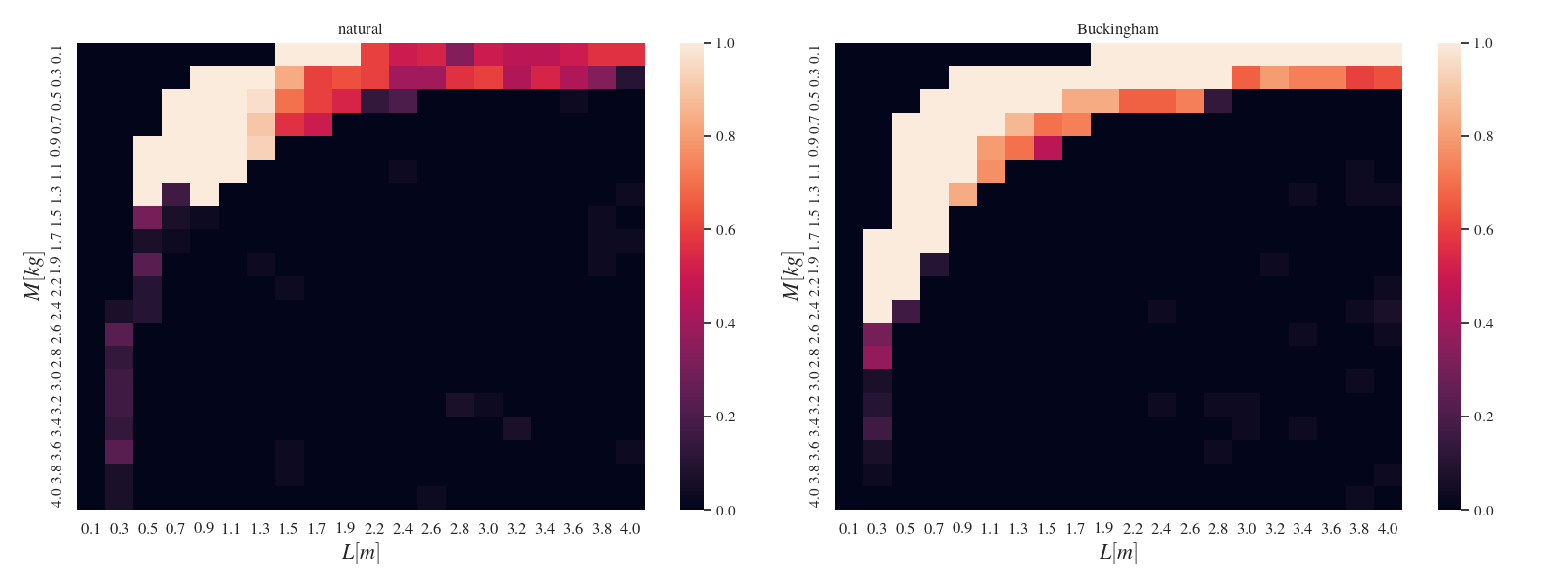
Figure 3: Pendulum success rates on the pole length when both $M$ and $L$ are varying for the natural (left) and dimensionless (right) controllers. Brighter values indicate higher success rates.

5 Experiments

Environment	$L[m]$	$M[kg]$	$g[m.s^{-2}]$
Pendulum	1	1	10
Cartpole	1	0.1	9.81

Table 2: Nominal context value for the cartpole and pendulum environments

We will evaluate our algorithm on two second-order systems, the first is the underactuated pendulum. The cartpole is a slightly more complicated one, where a pendulum is attached to a cart on a horizontal axis that can move left and right to stabilize the pole vertically up. The nominal context values for each are summarized in table 2.

These two systems possess the appealing properties of having smooth dynamics and low dimensions. As such, they are well suited for studying dimensional analysis in RL. The control policy is parameterized as a single-layer Radial Basis Function network. We use Moment Matching (Girard et al. 2002) for trajectory predictions as in the original PILCO paper. For the cartpole, we used the benchmark for distribution shift from (Dulac-Arnold et al. 2021b) and adapted some of the code for our needs. For the pendulum, we used Gymnasium (Towers et al. 2023) on which context variables can be changed with no code modification.

We use two different metrics to evaluate the generalization capabilities of our algorithm. The return (1) is the most commonly used metric used in Markov Decision Processes. It measures the long-term performance of a controller given an initial state distribution and is computed by a discounted sum of rewards. The reward for our environments are inversely proportional to the distance from the current state and target

$$r_{t}\propto-d(s_{t},s^{*}),$$ (16)

where $d$ is a distance function in $\mathcal{S}$. For our specific problems, we only consider finite-time MDPs and thus consider a discount rate $\gamma=1$, which weights identically the rewards from the beginning to end of each episode.

However, during the experiments we realized that this metric was not sufficient to characterise the ability of the controller to stabilize the systems. The return translates the ability of the agent to stabilize a system at a target position as quickly as possible, which ignores two components of our tasks. The first is that if two controllers are able to solve the task but one requires more steps to do so, it will be penalized with a lower return since it spends less time in the optimal-rewards regions. The second inconvenience is that if the controller is able to push the system into a closed-loop equilibrium that deviates from the target, it will not receive an optimal return. In the next section, we will illustrate these two points for each of the environments we studied.

In order to alleviate the bias of the return metric, we had to find a metric that would translate the ability of the controller to reach a closed-loop equilibrium. Therefore, we include a binary metric that measures whether in the last step of the episode, the velocity variables of the observations are equal to 0. We call such an episode successful, which allows us to measure the rate of successes for each controller across many different initializations. Our measure of success rate can be written as

$$\rho=\frac{1}{N}\sum_{i=1}^{N}\mathds{1}\left\{\dot{s_{T}}\leq\epsilon\right\},$$ (17)

where $N$ is the number of evaluation episodes and $\epsilon$ a threshold. For our experiments, we used the values $N=100$ and $\epsilon=0.05$.

Generalization Score

We consider the context is the 2-dimensional vector of mass and length. We consider perturbations that scale the context vector by a factor $a\in[0.5,1.5]$ of the nominal context as ${\bm{c}}=a{\bm{c}}_{0}$. For the pendulum on figure 3, both mass $M$ and length $L$ are perturbed around their nominal values. Bright colours indicate higher return, meaning good generalization of the controller, whereas dark ones indicate failure to stabilize the system. The first thing we notice is that even in the natural case, the policy for the pendulum is already able to generalize to a significant range of values. We hypothesize that this is due to the probabilistic nature of the policy search, which presents naturally robust capabilities (Charvet, Jensen, and Murray-Smith 2021). Nevertheless, the Buckingham transformation is able to enlarge this region, allowing large values of $L$ when is small (below 0.5). It also allows larger $M$ values, up to 2.4 when $L$ is smaller than 0.9. The same experiment for the cartpole is presented in figure 4.

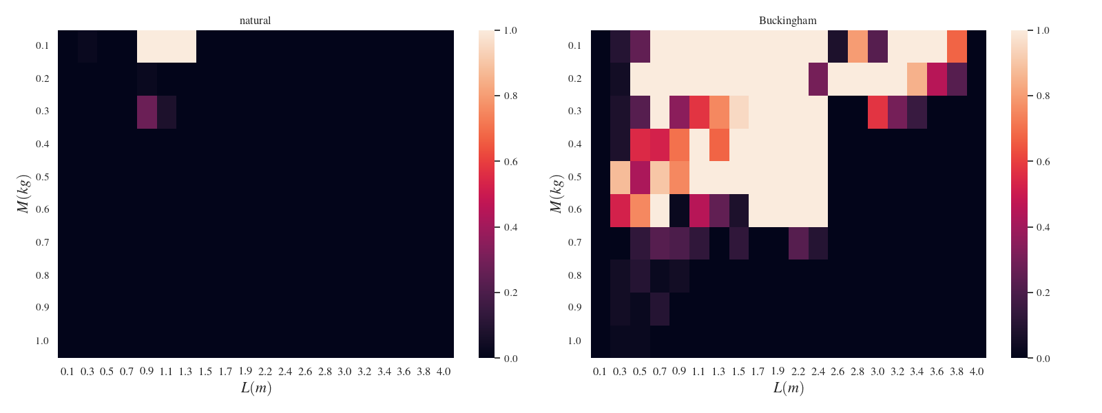
Figure 4: Cartpole success rates when both parameters $L$ and $M$ change simultaneously. We can see how the dimensionless controller (right) can solve the task on a much wider set of context pairs.

Following the idea of complementing the return metric, we propose another metric that is specific to the problem of generalization and robustness. We call controllable area the surface in parameter space on which the performance of the controller drops by a given fraction $\tau\in[0,1]$. The area can be mathematically described as follows,

$$\mathcal{S}_{control}(\tau)=\left\{{\bm{c}}\in{\mathcal{C}},~R_{\pi}({\bm{c}})\geq\tau R^{*}(\pi)\right\}.$$ (18)

This definition allows us to measure the region in context space in which the controller works close to its optimal regime. We can compute that value with means of an integral over the rate of episodes that have returns greater than the threshold for each infinitesimal context as,

$$\mathcal{S}_{control}(\tau)=\int_{\mathcal{C}}\mathds{1}[R_{\pi}({\bm{c}})\geq\tau R^{*}(\pi)]d{\bm{c}}.$$ (19)

We plot this area as a function of the performance dropoff $\tau$ on figure 5 for the pole mass and length. This figure confirms the findings from above, as we can see the area of optimality of the controllers is much larger for the one in dimensionless space. Note that depending on the system at hand, the controllable region may not be compact set of the context space. It is a similar phenomenon that we observe on figure 4.

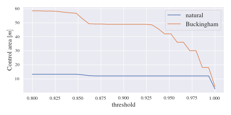
(a) Pole length

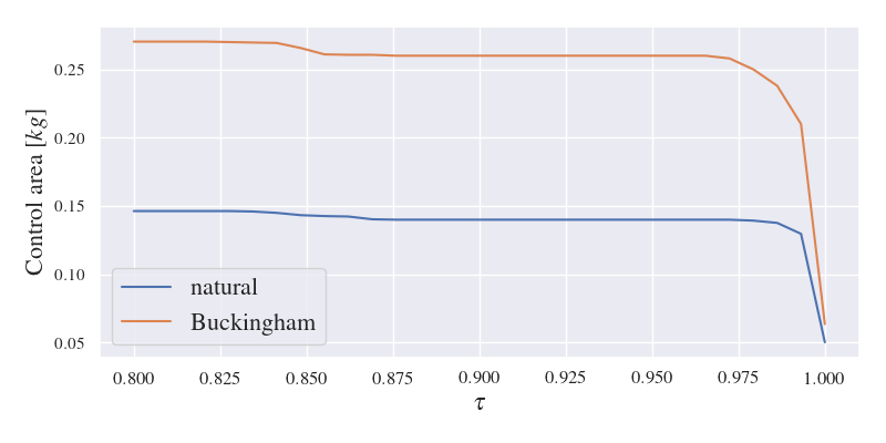
(b) Pole mass

Figure 5: Control area (18) pole length and mass. Higher values on the $x$-axis indicate better generalization.

Action Equivariance

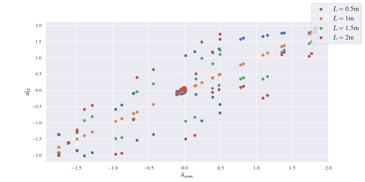
Figure 6: We plot the actions by the nominal controller ($x$-axis) against the perturbed ones ($y$-axis) for different pole lengths. All the controllers share the same natural input, but it is transformed by the context-dependent $\Pi$-groups.

We sample a subset of 100 one-step transitions from the data collected during training. We then plot the controller actions with the input state going through the Buckingham power-law transformation with appropriate context. As the environment undergoes a scaling transformation of the context, the dimensionless control actions are also scaled accordingly. On the other hand, the natural controller is agnostic to the context change and thus not able to stabilize the cartpole and solve the task. This phenomenon is highlighted on figure 6. Here we plot the natural against dimensionless controllers actions on the same sample of state data, but for different contexts. As we can see, the Buckingham actions are rescaled to reflect the change in pole length. This ability to transform the controller input further explains how zero-shot generalization can be improved with no additional training data.

6 Discussion

In this work, we investigated the problem of controller generalization when a dynamic system is subjected to environmental perturbations. We introduced the dimensionless Markov Decision Process in section 4, which allows an autonomous agent to take actions in a dimensionless observation space. The $\Pi$-MDP is a rescaling of a C-MDP state and action spaces such that each variable becomes dimensionless. The resulting state-action space stems from additional assumptions about the units of the system and the observation of perturbing variables. The equivariance properties of the transformation allow zero-shot transfer from one context to another.

From the $\Pi$-MDP formulation, we derived a generic framework for model-based policy search that we applied with a Gaussian Process dynamics model (algorithms 1 and 2). The new algorithm we proposed, built on top of PILCO, maintains its data-efficency and improves greatly its generalization capabilities with no further data collection.

We demonstrated empirically that this approach yields controllers that are invariant with respect to the context, provided it can be observed or measured. Our experiments focused on two different environments, an underactuated pendulum (figure 3) and a cartpole (figure 4). Our results show strong generalization properties of the controller when the physical properties of the system, such as pole length and mass, drift from their initial training value. While these are simple systems, because of their second-order dynamics and low dimension, the consistency of the results suggests the methodology could be successfully applied to more complex systems, which we leave to future work.

Conceptually, our approach comes within the scope of instilling physics prior knowledge in Machine Learning pipelines to increase model robustness (Botev et al. 2021). The main weakness of this approach is the requirement for measuring what the perturbation variables are at any point in the deployment of the controller. We believe identification of the parameters could be achieved with different control policies that aim to actively infer those values based on exploratory trajectories and leave this direction for future work. The second limitation of this approach is the requirement for knowing the measurements’ dimensions which can be prohibitively expensive on high-dimensional systems. To alleviate this, one could either use physical priors to determine which transformation is most suited to type of perturbation that might be later encountered or find them numerically as in (Bakarji et al. 2022).

Appendix A Pendulum $\Pi$-groups

Dynamic variables

$$\begin{cases}u:&\begin{bmatrix}1&1&-2\end{bmatrix}\\ \theta:&\begin{bmatrix}0&0&0\end{bmatrix}\\ \dot{\theta}:&\begin{bmatrix}0&0&-1\end{bmatrix}\\ \ddot{\theta}:&\begin{bmatrix}0&0&-2\end{bmatrix}\\ \end{cases}$$ (20)

Context

$$\begin{cases}M:&\begin{bmatrix}1&0&0\end{bmatrix}\\ g:&\begin{bmatrix}0&1&-2\end{bmatrix}\\ L:&\begin{bmatrix}0&1&0\end{bmatrix}\\ \end{cases}$$ (21)

The context matrix

$${\bm{C}}=\begin{bmatrix}1&0&0\\ 0&1&-2\\ 0&1&0\end{bmatrix}$$ (22)

is full rank and thus the variables $(M,g,L)$ can be used for non-dimensionalizing the other ones.

$$\begin{cases}\left[u^{\alpha_{u}}\cdot M^{\beta_{u}}\cdot g^{\delta_{u}}\cdot L^{\gamma_{u}}\right]=0\\ \left[\theta^{\alpha_{\theta}}\cdot M^{\beta_{\theta}}\cdot g^{\delta_{\theta}}\cdot L^{\gamma_{\theta}}\right]=0\\ \left[\dot{\theta}^{\alpha_{\dot{\theta}}}\cdot M^{\beta_{\dot{\theta}}}\cdot g^{\delta_{\dot{\theta}}}\cdot L^{\gamma_{\dot{\theta}}}\right]=0\\ \left[\ddot{\theta}^{\alpha_{\ddot{\theta}}}\cdot M^{\beta_{\ddot{\theta}}}\cdot g^{\delta_{\ddot{\theta}}}\cdot L^{\gamma_{\ddot{\theta}}}\right]=0\\ \end{cases}$$ (23)

Where the bracket signs $\left[x\right]$ represent the dimension of variable $x$ and each power law within equation 23 will be the $\Pi$-groups.

Because we know the dimension of the variables $u,\theta,\dot{\theta},\ddot{\theta}$ and because $[x\times y]=[x]\times[y]$ the system can be rewritten as

$$\begin{cases}M^{\beta_{u}}\cdot L^{\alpha_{u}+\delta_{u}+\gamma_{u}}\cdot t^{-2\delta_{u}+\alpha_{u}}=1\\ M^{\beta_{\dot{\theta}}}\cdot L^{\delta_{\dot{\theta}}+\gamma_{\dot{\theta}}}\cdot t^{-2\delta_{\dot{\theta}}-1}=1\\ M^{\beta_{\ddot{\theta}}}\cdot L^{\delta_{\ddot{\theta}}+\gamma_{\ddot{\theta}}}\cdot t^{-2\delta_{\dot{\theta}}-2}=1\end{cases}$$ (24)

We removed the equation for $\theta$ because as an angle, this variable is naturally dimensionless. The coefficients are found by solving one system for each variable.

Torque $u$

$\Pi_{u}=u^{\alpha}\cdot M^{\beta}\cdot g^{\delta}\cdot L^{\gamma}$ Using the first term from 24 and replacing the terms by their dimension we obtain,

$$M^{\alpha+\beta}.L^{\alpha+\delta+\gamma}t^{-2\alpha-2\delta}=1.$$ (25)

All exponents must be 0 to ensure the homogeneity which yields

$$\begin{cases}\alpha+\beta&=0\\ \alpha+\delta+\gamma&=0\\ \alpha-2\delta&=0\end{cases}$$ (26)

The last equation implies $\alpha+\delta=0$, which we substract from the first equation to obtain

$$\begin{cases}\beta=\delta\\ \alpha+\beta=0\\ \alpha+\delta+\gamma=0,\end{cases}$$ (27)

and then using $\alpha+\delta=0$

$$\begin{cases}\beta=\delta\gamma=0\\ \alpha+\beta=0.\\ \end{cases}$$ (28)

Because the solution is not unique, we choose $\alpha=1$, which gives the dimensionless torque

$$\Pi_{u}=\frac{u}{Mg}.$$ (29)

Angular speed $\dot{\theta}$

$\Pi_{\dot{\theta}}=\dot{\theta}^{\alpha}\cdot M^{\beta}\cdot g^{\delta}\cdot L^{\gamma}$ We replace the variables with their dimensions to obtain

$$M^{\beta}.L^{\delta+\gamma}.t^{-\alpha-2\delta}=1,$$ (30)

which we can solve with the systems

$$\begin{cases}\beta=0\\ \delta+\gamma=0\\ \alpha+2\delta=0.\end{cases}$$ (31)

By subtracting twice the second equation from the third we obtain

$$\begin{cases}\beta=0\\ \alpha=2\gamma\\ \delta+\gamma=0.\end{cases}$$ (32)

We choose $\delta=1$ yielding

$$\Pi_{\dot{\theta}}=\dot{\theta}^{2}\dfrac{g}{L}.$$ (33)

Angular acceleration $\ddot{\theta}$

By the same process we obtain,

$$M^{\beta}.L^{\delta+\gamma}.t^{-\alpha-2\delta}=1,$$ (34)

$\beta=0$, so we have the systems

$$\begin{cases}\delta+\gamma=0\\ \alpha=\beta.\end{cases}$$ (35)

This yields

$$\Pi_{\ddot{\theta}}=\ddot{\theta}\frac{g}{L}.$$ (36)

Appendix B Cartpole $\Pi$-groups

The movement of the cartpole depends on the variables $(x,\cos(\theta),\sin(\theta),\dot{x},\dot{\theta}),u$. A trivial $\Pi$-group for the cart position is $\Pi_{x}=\dfrac{x}{L}$, where $L$ is the pole length. For the angular speed, we use the same transformation as the pendulum. Therefore, we need to compute the dimensionless variables for $\dot{x}$ and $u$

Cart speed $\dot{x}$

With $\Pi_{\dot{x}}=\dot{x}^{\alpha}\cdot M^{\beta}\cdot g^{\delta}\cdot L^{\gamma}$, we obtain with $[\dot{x}]=L.t^{-1}$,

$$M^{\beta}.L^{\alpha+\delta+\gamma}.t^{-\alpha-2\delta}$$ (37)

which yields $\beta=0$. We then substract on equation with the other to obtain,

$$\begin{cases}\delta-\gamma=0\\ \alpha+2\delta=0,\end{cases}$$ (38)

which is solved with $\delta=\gamma=-1$. Therefore the dimensionless variable for the cart is

$$\Pi_{\dot{x}}=\dfrac{\dot{x}^{2}}{Lg}.$$ (39)

Force $u$

$\Pi_{u}=u^{\alpha}\cdot M^{\beta}\cdot g^{\delta}\cdot L^{\gamma}$ The dimension of the control force is $[u]=M.L.t^{-2}$. Using that value yields the system

$$\begin{cases}\alpha+\beta=0\\ \alpha+\delta=0\\ \alpha+\delta+\gamma=0\end{cases}$$ (40)

and by substracting the first two equations we obtain

$$\begin{cases}\gamma=0\\ \beta=\delta\\ \alpha+\delta=0.\end{cases}$$ (41)

With $\alpha=1$, we obtain the resulting

$$\Pi_{u}=\dfrac{u}{Mg}.$$ (42)

References

- Amadio et al. (2022) Amadio, F.; Dalla Libera, A.; Antonello, R.; Nikovski, D. N.; Carli, R.; and Romeres, D. 2022. Model-Based Policy Search Using Monte Carlo Gradient Estimation with Real Systems Application. IEEE Transaction on Robotics, 38(6): 3879–3898.
- Bakarji et al. (2022) Bakarji, J.; Callaham, J.; Brunton, S. L.; and Kutz, J. N. 2022. Dimensionally consistent learning with Buckingham Pi. Nature Computational Science, 2(12): 834–844.
- Ball et al. (2021) Ball, P. J.; Lu, C.; Parker-Holder, J.; and Roberts, S. 2021. Augmented World Models Facilitate Zero-Shot Dynamics Generalization From a Single Offline Environment. In Meila, M.; and Zhang, T., eds., Proceedings of the 38th International Conference on Machine Learning, volume 139 of Proceedings of Machine Learning Research, 619–629. PMLR.
- Botev et al. (2021) Botev, A.; Jaegle, A.; Wirnsberger, P.; Hennes, D.; and Higgins, I. 2021. Which priors matter? Benchmarking models for learning latent dynamics. In Vanschoren, J.; and Yeung, S., eds., Proceedings of the Neural Information Processing Systems Track on Datasets and Benchmarks, volume 1. Curran.
- Buckingham (1914) Buckingham, E. 1914. On physically similar systems; illustrations of the use of dimensional equations. Physical review, 4(4): 345.
- Charvet, Jensen, and Murray-Smith (2021) Charvet, V.; Jensen, B. S.; and Murray-Smith, R. 2021. Learning Robust Controllers Via Probabilistic Model-Based Policy Search. In International Conference on Learning Representations - Robust ML Workshop.
- Chua et al. (2018) Chua, K.; Calandra, R.; McAllister, R.; and Levine, S. 2018. Deep Reinforcement Learning in a Handful of Trials using Probabilistic Dynamics Models. In Bengio, S.; Wallach, H.; Larochelle, H.; Grauman, K.; Cesa-Bianchi, N.; and Garnett, R., eds., Advances in Neural Information Processing Systems, volume 31. Curran Associates, Inc.
- Cowen-Rivers et al. (2022) Cowen-Rivers, A. I.; Palenicek, D.; Moens, V.; Abdullah, M. A.; Sootla, A.; Wang, J.; and Bou-Ammar, H. 2022. Samba: Safe model-based & active reinforcement learning. Machine Learning, 111(1): 173–203.
- Deisenroth and Rasmussen (2011) Deisenroth, M. P.; and Rasmussen, C. E. 2011. PILCO: A Model-Based and Data-Efficient Approach to Policy Search. In International Conference on Machine Learning. 467-472.
- Derman et al. (2020) Derman, E.; Mankowitz, D.; Mann, T.; and Mannor, S. 2020. A Bayesian Approach to Robust Reinforcement Learning. In Adams, R. P.; and Gogate, V., eds., Proceedings of The 35th Uncertainty in Artificial Intelligence Conference, volume 115 of Proceedings of Machine Learning Research, 648–658. PMLR.
- Doshi-Velez and Konidaris (2016) Doshi-Velez, F.; and Konidaris, G. 2016. Hidden parameter markov decision processes: A semiparametric regression approach for discovering latent task parametrizations. In IJCAI: proceedings of the conference, volume 2016, 1432. NIH Public Access.
- Dulac-Arnold et al. (2021a) Dulac-Arnold, G.; Levine, N.; Mankowitz, D. J.; Li, J.; Paduraru, C.; Gowal, S.; and Hester, T. 2021a. Challenges of real-world Reinforcement Learning: definitions, benchmarks and analysis. Machine Learning, 110(9): 2419–2468.
- Dulac-Arnold et al. (2021b) Dulac-Arnold, G.; Levine, N.; Mankowitz, D. J.; Li, J.; Paduraru, C.; Gowal, S.; and Hester, T. 2021b. An empirical investigation of the challenges of real-world Reinforcement Learning. arXiv:2003.11881.
- Eysenbach and Levine (2021) Eysenbach, B.; and Levine, S. 2021. Maximum Entropy RL (Provably) Solves Some Robust RL Problems. In International Conference on Learning Representations.
- Ghosh et al. (2021) Ghosh, D.; Rahme, J.; Kumar, A.; Zhang, A.; Adams, R. P.; and Levine, S. 2021. Why Generalization in RL is Difficult: Epistemic POMDPs and Implicit Partial Observability. In Ranzato, M.; Beygelzimer, A.; Dauphin, Y.; Liang, P.; and Vaughan, J. W., eds., Advances in Neural Information Processing Systems, volume 34, 25502–25515. Curran Associates, Inc.
- Girard (2024) Girard, A. 2024. Dimensionless Policies Based on the Buckingham Theorem: Is This a Good Way to Generalize Numerical Results? Mathematics, 12(5).
- Girard et al. (2002) Girard, A.; Rasmussen, C.; Quiñonero Candela, J.; and Murray-Smith, R. 2002. Gaussian Process Priors with Uncertain Inputs Application to Multiple-Step Ahead Time Series Forecasting. In Becker, S.; Thrun, S.; and Obermayer, K., eds., Advances in Neural Information Processing Systems, volume 15. MIT Press.
- Hallak, Castro, and Mannor (2015) Hallak, A.; Castro, D. D.; and Mannor, S. 2015. Contextual Markov Decision Processes. arXiv:1502.02259.
- Hishinuma and Senda (2021) Hishinuma, T.; and Senda, K. 2021. Weighted model estimation for offline model-based Reinforcement Learning. In Ranzato, M.; Beygelzimer, A.; Dauphin, Y.; Liang, P.; and Vaughan, J. W., eds., Advances in Neural Information Processing Systems, volume 34, 17789–17800. Curran Associates, Inc.
- Hong et al. (2023) Hong, Z.-W.; Kumar, A.; Karnik, S.; Bhandwaldar, A.; Srivastava, A.; Pajarinen, J.; Laroche, R.; Gupta, A.; and Agrawal, P. 2023. Beyond Uniform Sampling: Offline Reinforcement Learning with Imbalanced Datasets. In Oh, A.; Naumann, T.; Globerson, A.; Saenko, K.; Hardt, M.; and Levine, S., eds., Advances in Neural Information Processing Systems, volume 36, 4985–5009. Curran Associates, Inc.
- Huang et al. (2023) Huang, P.; Zhang, X.; Cao, Z.; Liu, S.; Xu, M.; Ding, W.; Francis, J.; Chen, B.; and Zhao, D. 2023. What Went Wrong? Closing the Sim-to-Real Gap via Differentiable Causal Discovery. In Tan, J.; Toussaint, M.; and Darvish, K., eds., Proceedings of The 7th Conference on Robot Learning, volume 229 of Proceedings of Machine Learning Research, 734–760. PMLR.
- Igl et al. (2019) Igl, M.; Ciosek, K.; Li, Y.; Tschiatschek, S.; Zhang, C.; Devlin, S.; and Hofmann, K. 2019. Generalization in Reinforcement Learning with Selective Noise Injection and Information Bottleneck. In Wallach, H.; Larochelle, H.; Beygelzimer, A.; d'Alché-Buc, F.; Fox, E.; and Garnett, R., eds., Advances in Neural Information Processing Systems, volume 32.
- Janner et al. (2019) Janner, M.; Fu, J.; Zhang, M.; and Levine, S. 2019. When to Trust Your Model: Model-Based Policy Optimization. In Wallach, H.; Larochelle, H.; Beygelzimer, A.; d'Alché-Buc, F.; Fox, E.; and Garnett, R., eds., Advances in Neural Information Processing Systems, volume 32. Curran Associates, Inc.
- Kansky et al. (2017) Kansky, K.; Silver, T.; Mély, D. A.; Eldawy, M.; Lázaro-Gredilla, M.; Lou, X.; Dorfman, N.; Sidor, S.; Phoenix, S.; and George, D. 2017. Schema Networks: Zero-shot Transfer with a Generative Causal Model of Intuitive Physics. In Precup, D.; and Teh, Y. W., eds., Proceedings of the 34th International Conference on Machine Learning, volume 70 of Proceedings of Machine Learning Research, 1809–1818. PMLR.
- Kidambi et al. (2020) Kidambi, R.; Rajeswaran, A.; Netrapalli, P.; and Joachims, T. 2020. MOReL: Model-Based Offline Reinforcement Learning. In Larochelle, H.; Ranzato, M.; Hadsell, R.; Balcan, M. F.; and Lin, H., eds., Advances in Neural Information Processing Systems, volume 33, 21810–21823. Curran Associates, Inc.
- Kim and Oh (2023) Kim, B.; and Oh, M.-H. 2023. Model-based Offline Reinforcement Learning with Count-based Conservatism. In Krause, A.; Brunskill, E.; Cho, K.; Engelhardt, B.; Sabato, S.; and Scarlett, J., eds., Proceedings of the 40th International Conference on Machine Learning, volume 202 of Proceedings of Machine Learning Research, 16728–16746. PMLR.
- Kingma and Welling (2014) Kingma, D. P.; and Welling, M. 2014. Auto-encoding variational Bayes. In International Conference on Learning Representaions.
- Kirk et al. (2023) Kirk, R.; Zhang, A.; Grefenstette, E.; and Rocktäschel, T. 2023. A survey of zero-shot generalisation in deep Reinforcement Learning. Journal of Artificial Intelligence Research, 76: 201–264.
- Kumar et al. (2018) Kumar, N.; Rajagopalan, P.; Pankajakshan, P.; Bhattacharyya, A.; Sanyal, S.; Balachandran, J.; and Waghmare, U. V. 2018. Machine learning constrained with dimensional analysis and scaling laws: simple, transferable, and interpretable models of materials from small datasets. Chemistry of Materials, 31(2): 314–321.
- Kupcsik et al. (2013) Kupcsik, A.; Deisenroth, M.; Peters, J.; and Neumann, G. 2013. Data-efficient generalization of robot skills with contextual policy search. In Proceedings of the AAAI conference on artificial intelligence, volume 27, 1401–1407.
- Kwon et al. (2021) Kwon, J.; Efroni, Y.; Caramanis, C.; and Mannor, S. 2021. RL for Latent MDPs: Regret Guarantees and a Lower Bound. In Ranzato, M.; Beygelzimer, A.; Dauphin, Y.; Liang, P.; and Vaughan, J. W., eds., Advances in Neural Information Processing Systems, volume 34, 24523–24534. Curran Associates, Inc.
- Lee, Zidek, and Heckman (2021) Lee, T. Y.; Zidek, J. V.; and Heckman, N. 2021. Dimensional Analysis in Statistical Modelling. arXiv preprint arXiv:2002.11259.
- Levine et al. (2020) Levine, S.; Kumar, A.; Tucker, G.; and Fu, J. 2020. Offline Reinforcement Learning: Tutorial, Review, and Perspectives on Open Problems. arXiv:2005.01643.
- Ljung (1989) Ljung, L. 1989. System identification-Theory for the user. 3. Pearson Education.
- Mankowitz et al. (2018) Mankowitz, D.; Mann, T.; Bacon, P.-L.; Precup, D.; and Mannor, S. 2018. Learning robust options. In Proceedings of the AAAI Conference on Artificial Intelligence, volume 32.
- Mankowitz et al. (2019) Mankowitz, D. J.; Levine, N.; Jeong, R.; Abdolmaleki, A.; Springenberg, J. T.; Shi, Y.; Kay, J.; Hester, T.; Mann, T.; and Riedmiller, M. 2019. Robust Reinforcement Learning for Continuous Control with Model Misspecification. In International Conference on Learning Representations.
- Mohamed et al. (2020) Mohamed, S.; Rosca, M.; Figurnov, M.; and Mnih, A. 2020. Monte Carlo Gradient Estimation in Machine Learning. Journal of Machine Learning Research, 21(132): 1–62.
- Morimoto and Doya (2005) Morimoto, J.; and Doya, K. 2005. Robust Reinforcement Learning. Neural computation, 17(2): 335–359.
- Muglich et al. (2022) Muglich, D.; Schroeder de Witt, C.; van der Pol, E.; Whiteson, S.; and Foerster, J. 2022. Equivariant Networks for Zero-Shot Coordination. In Koyejo, S.; Mohamed, S.; Agarwal, A.; Belgrave, D.; Cho, K.; and Oh, A., eds., Advances in Neural Information Processing Systems, volume 35, 6410–6423. Curran Associates, Inc.
- Oppenheimer, Doman, and Merrick (2023) Oppenheimer, M. W.; Doman, D. B.; and Merrick, J. D. 2023. Multi-scale physics-informed machine learning using the Buckingham Pi theorem. Journal of Computational Physics, 474: 111810.
- Parmas et al. (2018) Parmas, P.; Rasmussen, C. E.; Peters, J.; and Doya, K. 2018. PIPPS: Flexible Model-Based Policy Search Robust to the Curse of Chaos. In Dy, J.; and Krause, A., eds., Proceedings of the 35th International Conference on Machine Learning, volume 80 of Proceedings of Machine Learning Research, 4065–4074. PMLR.
- Pinto et al. (2017) Pinto, L.; Davidson, J.; Sukthankar, R.; and Gupta, A. 2017. Robust adversarial Reinforcement Learning. In International Conference on Machine Learning, 2817–2826.
- Sæmundsson, Hofmann, and Deisenroth (2018) Sæmundsson, S.; Hofmann, K.; and Deisenroth, M. 2018. Meta Reinforcement Learning with latent variable Gaussian processes. In 34th Conference on Uncertainty in Artificial Intelligence 2018, UAI 2018, volume 34, 642–652. Association for Uncertainty in Artificial Intelligence (AUAI).
- Schrittwieser et al. (2020) Schrittwieser, J.; Antonoglou, I.; Hubert, T.; Simonyan, K.; Sifre, L.; Schmitt, S.; Guez, A.; Lockhart, E.; Hassabis, D.; Graepel, T.; et al. 2020. Mastering Atari, Go, chess and shogi by planning with a learned model. Nature, 588(7839): 604–609.
- Sculley et al. (2015) Sculley, D.; Holt, G.; Golovin, D.; Davydov, E.; Phillips, T.; Ebner, D.; Chaudhary, V.; Young, M.; Crespo, J.-F.; and Dennison, D. 2015. Hidden Technical Debt in Machine Learning Systems. In Cortes, C.; Lawrence, N.; Lee, D.; Sugiyama, M.; and Garnett, R., eds., Advances in Neural Information Processing Systems, volume 28. Curran Associates, Inc.
- Shen and Lin (2018) Shen, W.; and Lin, D. K. J. 2018. A Conjugate Model for Dimensional Analysis. Technometrics, 60(1): 79–89.
- Shen and Lin (2019) Shen, W.; and Lin, D. K. J. 2019. Statistical Theories For Dimensional Analysis. Statistica Sinica, 29(2): 527–550.
- Sonin (2001) Sonin, A. A. 2001. Dimensional analysis. Technical report, Department of Mechanical Engineering - MIT.
- Tamar, Mannor, and Xu (2014) Tamar, A.; Mannor, S.; and Xu, H. 2014. Scaling Up Robust MDPs using Function Approximation. In Xing, E. P.; and Jebara, T., eds., Proceedings of the 31st International Conference on Machine Learning, volume 32 of Proceedings of Machine Learning Research, 181–189. Bejing, China.
- Therrien, Lecompte, and Girard (2024) Therrien, W.; Lecompte, O.; and Girard, A. 2024. Using the Buckingham Theorem for Multi-System Transfer Learning: A Case-Study with 3 Vehicles Sharing a Database. Electronics, 13(11).
- Towers et al. (2023) Towers, M.; Terry, J. K.; Kwiatkowski, A.; Balis, J. U.; Cola, G. d.; Deleu, T.; Goulão, M.; Kallinteris, A.; KG, A.; Krimmel, M.; Perez-Vicente, R.; Pierré, A.; Schulhoff, S.; Tai, J. J.; Shen, A. T. J.; and Younis, O. G. 2023. Gymnasium.
- Unbehauen (2000) Unbehauen, H. 2000. Adaptive dual control systems: a survey. In Proceedings of the IEEE 2000 Adaptive Systems for Signal Processing, Communications, and Control Symposium (Cat. No.00EX373), 171–180.
- van der Pol et al. (2021) van der Pol, E.; van Hoof, H.; Oliehoek, F. A.; and Welling, M. 2021. Multi-Agent MDP Homomorphic Networks. In International Conference on Learning Representations.
- Villar et al. (2023) Villar, S.; Yao, W.; Hogg, D. W.; Blum-Smith, B.; and Dumitrascu, B. 2023. Dimensionless machine learning: Imposing exact units equivariance. Journal of Machine Learning Research, 24(109): 1–32.
- Wiesemann, Kuhn, and Rustem (2013) Wiesemann, W.; Kuhn, D.; and Rustem, B. 2013. Robust Markov Decision Processes. Mathematics of Operations Research, 38(1): 153–183.
- Williams (1992) Williams, R. J. 1992. Simple Statistical Gradient-Following Algorithms for Connectionist Reinforcement Learning, 5–32. Boston, MA: Springer US. ISBN 978-1-4615-3618-5.
- Xu et al. (2019) Xu, M.; Quiroz, M.; Kohn, R.; and Sisson, S. A. 2019. Variance reduction properties of the reparameterization trick. In Chaudhuri, K.; and Sugiyama, M., eds., Proceedings of the Twenty-Second International Conference on Artificial Intelligence and Statistics, volume 89 of Proceedings of Machine Learning Research, 2711–2720. PMLR.
- Yang, Ze, and Xu (2023) Yang, S.; Ze, Y.; and Xu, H. 2023. MoVie: Visual Model-Based Policy Adaptation for View Generalization. In Oh, A.; Naumann, T.; Globerson, A.; Saenko, K.; Hardt, M.; and Levine, S., eds., Advances in Neural Information Processing Systems, volume 36, 21507–21523. Curran Associates, Inc.
- Yu et al. (2020) Yu, T.; Thomas, G.; Yu, L.; Ermon, S.; Zou, J. Y.; Levine, S.; Finn, C.; and Ma, T. 2020. MOPO: Model-based Offline Policy Optimization. In Larochelle, H.; Ranzato, M.; Hadsell, R.; Balcan, M. F.; and Lin, H., eds., Advances in Neural Information Processing Systems, volume 33, 14129–14142. Curran Associates, Inc.
- Yuan et al. (2023) Yuan, Y.; Chen, C. S.; Liu, Z.; Neiswanger, W.; and Liu, X. S. 2023. Importance-aware Co-teaching for Offline Model-based Optimization. In Oh, A.; Naumann, T.; Globerson, A.; Saenko, K.; Hardt, M.; and Levine, S., eds., Advances in Neural Information Processing Systems, volume 36, 55718–55733. Curran Associates, Inc.
- Zhu et al. (2023) Zhu, C.; Simchowitz, M.; Gadipudi, S.; and Gupta, A. 2023. RePo: Resilient Model-Based Reinforcement Learning by Regularizing Posterior Predictability. In Oh, A.; Naumann, T.; Globerson, A.; Saenko, K.; Hardt, M.; and Levine, S., eds., Advances in Neural Information Processing Systems, volume 36, 32445–32467. Curran Associates, Inc.