Bipartite Matching is in Catalytic Logspace
Abstract
Matching is a central problem in theoretical computer science,
with a large body of work spanning the last five decades.
However, understanding matching in the time-space bounded setting
remains a longstanding open question, even in the presence of additional
resources such as randomness or non-determinism.
In this work we study space-bounded machines with access to catalytic space,
which is additional working memory that is full with arbitrary data that
must be preserved at the end of its computation. Despite this heavy restriction,
many recent works have shown the power of catalytic space,
its utility in designing classical space-bounded algorithms,
and surprising connections between catalytic computation and derandomization.
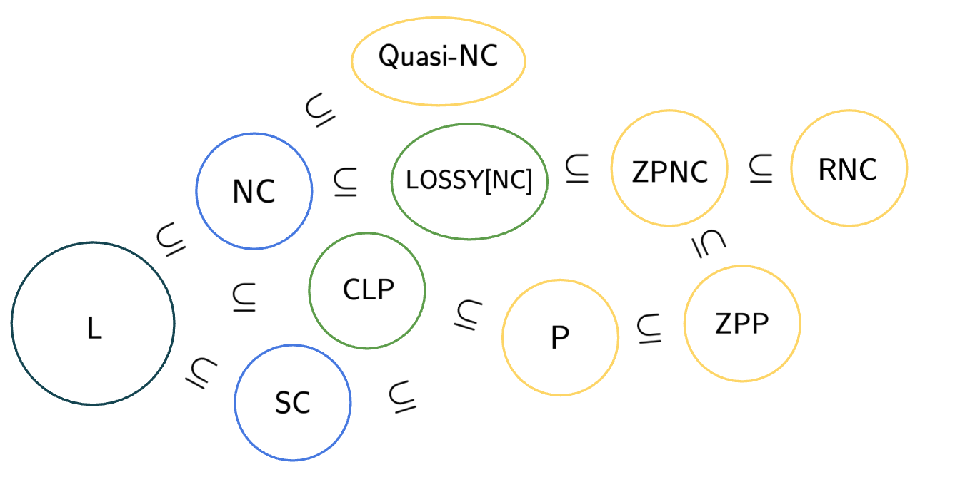
Our main result is that bipartite maximum matching (MATCH) can be computed in catalytic logspace (CL) with a polynomial time bound (CLP). Moreover, we show that MATCH can be reduced to the lossy coding problem for NC circuits (LOSSY[NC]). This has consequences for matching, catalytic space, and derandomization:
-
•
Matching: this is the first well studied subclass of P which is known to compute MATCH, as well as the first algorithm simultaneously using sublinear free space and polynomial time with any additional resources. Thus, it gives a potential path to designing stronger space and time-space bounded algorithms.
-
•
Catalytic space: this is the first new problem shown to be in CL since the model was defined, and one which is extremely central and well-studied. Furthermore, it implies a strong barrier to showing CL lies anywhere in the NC hierarchy, and suggests to the contrary that CL is even more powerful than previously believed.
-
•
Derandomization: we give the first class beyond L for which we exhibit a natural problem in LOSSY[] which is not known to be in , as well as a full derandomization of the isolation lemma in CL in the context of MATCH. This also suggests a possible approach to derandomizing the famed RNC algorithm for MATCH.
Our proof combines a number of strengthened ideas from isolation-based algorithms for matching alongside the compress-or-random framework in catalytic computation.
1 Introduction
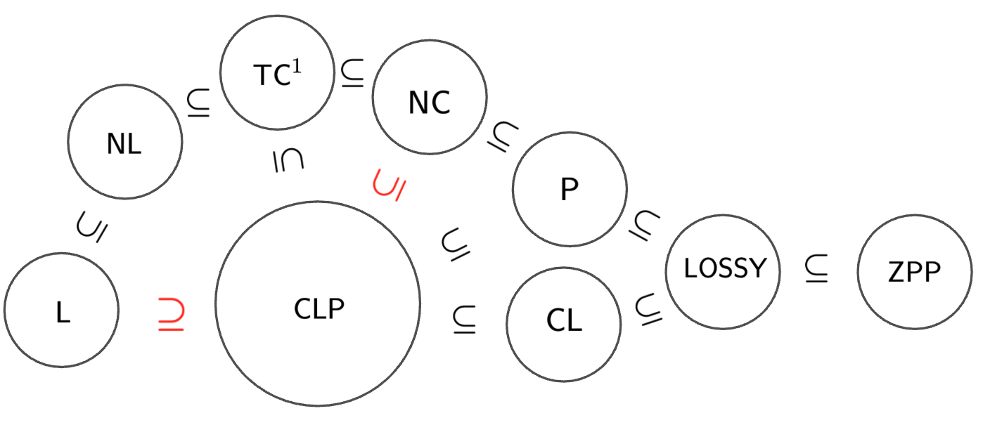
In this work we study a number of key questions and models of complexity between logarithmic space (L) and polynomial time (P). In particular we focus on the relationship between bipartite maximum matching (MATCH) and poly-time bounded catalytic logspace (CLP), as well as their implications for efficient parallel algorithms (NC) and efficient time-space algorithms (). Lastly we draw on connections between both MATCH and CLP to problems in derandomization—for the former we focus on the isolation lemma, and with regards to the latter we discuss reductions to the lossy coding problem—to make progress therein.
1.1 Matching and catalytic computation
Matching.
In the MATCH problem, we are given a bipartite graph as input and our goal is to return a subset of edges of maximum size such that no two edges share an endpoint. MATCH has been a central problem in the study of complexity since its inception, and was one of the earliest problems to be studied with respect to time; it has been known for 70 years that MATCH can be solved in P [Kuh55, HK73]. However, we are not aware of any well-studied class111Throughout this paper, when we discuss classes containing MATCH we ignore granular poly-time classes which immediately follow as a direct consequence of the above algorithms, e.g. , or those that contain matching by definition, i.e. the class of problems reducible to MATCH. such that .
Question 1: Is MATCH in any subclass of P?
For two such classes in particular, namely NC and SC, proving this would be a major breakthrough [Lov79, KUW85, MVV87, ARZ99, MV00, DKR10, FGT16, ST17, AV19, GG17, MN89, AV20, BBRS98]. With regards to parallel complexity, a long line of work culminated in showing that MATCH can be solved in randomized NC (RNC) [MVV87] and in quasi-polynomial size NC (Quasi-NC) [FGT16], but despite decades of research no true NC algorithms are known to this day.
Question 2: Is ?
Matching holds an even more central place in the study of space and time-space efficiency. It is widely conjectured that logarithmic space is insufficient to solve MATCH (i.e. ), and proving so would give a breakthrough separation between L and P. Similarly, with regards to time-space complexity we have no algorithms which compute MATCH in polynomial time and sublinear space even given additional resources such as non-determinism or randomness, and it is unclear whether such algorithms should exist or not.
Question 3: Do there exist any resources such that
?
In this work we study another such class called catalytic logspace (CL), and in particular its poly-time variant CLP, which is of great interest in relation to both NC and SC. In doing so we give a first-ever solution to Questions 1 and 3, as well as a potential barrier—or approach—to resolving Question 2.
Catalytic computing.
In catalytic computing, a space-bounded machine is given additional access to a much longer “catalytic” tape, which is additional memory already full of arbitrary data whose contents must be preserved by the computation. CL is the class of problems solvable by a logspace machine augmented with a polynomial length catalytic tape, and CLP is the subclass of CL where the machine is additionally required to run in polynomial time.
The framework of catalytic computation was formally introduced by Buhrman et al. [BCK+14] in order to understand the power of additional but used memory. It was informally conjectured earlier, in the context of the tree evaluation problem [CMW+12], that used memory could not grant additional power to space bounded machines. However, [BCK+14] showed that CL and even CLP contain problems believed to not be in L:
In the same work, they state that it is unclear what their result implies about the strength of CL. Particularly, is , or is the intuition that catalytic space does not grant additional power indeed correct, thus giving an approach to proving ?
Question 4: Where does CL lie between L and ZPP?
Since their result, many works have studied the utility and power of
catalytic computation (see e.g. [BKLS18, GJST19, DGJ+20, BDS22, CM22, Pyn24, CLMP25, GJST24, FMST25, PSW25, KMPS25]).
These results and techniques have also seen applications for ordinary
space-bounded computation, such as 1) work on the Tree Evaluation Problem
by Cook and Mertz [CM20, CM21, CM24] as well as a
subsequent breakthrough by Williams [Wil25] for simulating time in low space; and
2) win-win arguments for derandomization and other questions in
logspace [DPT24, LPT24, Pyn24] such as a recent result
of Doron et al. [DPTW25] showing that, in an instance-wise
fashion, either or . We refer
the interested reader to surveys of Koucký [Kou16] and Mertz [Mer23]
for more discussion.
However, despite all of the aforementioned work, no problems outside of TC1 have been shown to be in CL222Li, Pyne, and Tell [LPT24] give a search problem in CL which is not known to be in TC1; however, unlike with MATCH, the corresponding decision problem is in TC1 and thus is not applicable for studying the power of CL with regards to decision problems.. Thus, it is still possible that , which has led to conjectures, such as that of [Kou16, Mer23], that CL can indeed be computed somewhere in the NC hierarchy.
Question 5: Is ?
Our results (1).
In this work we address and connect all of the aforementioned questions by showing that catalytic logspace can compute bipartite matching in polynomial time:
Theorem 1.1.
We make a few notes on the power of Theorem 1.1:
-
1.
This is the first subclass of P which has been shown to contain MATCH (Question 1).
-
2.
This is the first algorithm for MATCH for any additional resources (Question 3). We believe that this gives hope for showing that MATCH can be computed in , or perhaps, as was the case with Tree Evaluation, such catalytic algorithms are a reason to doubt our intuition that MATCH cannot be solved in space altogether.
-
3.
This is the first problem outside TC1 shown to be in CL, and thus the first strengthening of CL since the original work of Buhrman et al. [BCK+14]; this also gives the strongest evidence thus far that (Question 4).
- 4.
-
5.
Many previous works have shown reductions from other graph problems to MATCH, and thus our CLP inclusion extends to these problems as well. We discuss the cases of weighted matching, - max-flow, and global min-cut in Section 7, although we stress this list is only a partial sample of such extensions of Theorem 1.1.
1.2 Derandomization
Lossy coding.
One other important, and useful, aspect of catalytic computation is a connection to fundamental questions in derandomization, a connection exploited in recent line of work [DPT24, LPT24, Pyn24, DPTW25] for showing novel non-catalytic space-bounded algorithms. The lossy coding problem [Kor22] is defined as follows: given a pair of circuits and , output such that . For a closed complexity class , LOSSY[] is the class of problems -reducible to lossy coding when Comp and Decomp are required to be computed and evaluated in the class . It is easy to see that
LOSSY[P], which is often just referred to as LOSSY,
has seen attention in recent years
in the context of total function NP [Kor22], range avoidance [KP24],
and meta-complexity [CLO+23], and was discussed at
length in a recent survey by Korten [Kor25] on the topic.
The problem of derandomizing LOSSY is seen as a stepping stone towards
the major derandomization goal of .
Unfortunately, for most classes it remains unclear whether LOSSY[] contains any natural and well studied problem outside . This was posed as an open problem in [Kor25].
Question 6: Does admit a natural problem not known to be in for any class ?
The only known progress on this question comes via catalytic computation, as Pyne [Pyn24] showed that . However, this remains unknown for all larger classes. Moreover, due to the fact that space-bounded randomized classes use read-once randomness, LOSSY[L] is perhaps an overkill for derandomizing BPL.
Isolation lemma.
One of the greatest contributions of the study of MATCH to complexity theory is a key tool, known as the isolation lemma, which is the backbone of all parallel algorithms for MATCH algorithms since its introduction by Mulmuley, Vazirani, and Vazirani [MVV87]. It has since turned out to be a very strong tool used in the design of randomized algorithms for a wide range of problems [OS93, LP15, NSV94, GT17, KS01, RA00, BTV09, KT16, VMP19, AM08] 333For a more comprehensive list of applications of the isolation lemma we direct the readers to [AGT20].. Thus, derandomizing the isolation lemma, independent of a concrete problem, has become an important problem in itself [CRS93, AM08, AGT20, AV20, GTV21].
Question 7: Which deterministic classes can implement the isolation lemma?
While the breakthrough Quasi-NC algorithm of Fenner, Gurjar, and Thierauf [FGT16] does exactly this, it both lies outside P and uses weights which are much larger than in all other applications. In fact this question is unresolved even for the “derandomization” class for NC discussed above, namely its LOSSY variant.
Question 8: Is the isolation lemma in LOSSY[NC]?
Our results (2).
An analysis of our algorithm in Theorem 1.1 gives answers to all of the above questions:
Theorem 1.2.
Again some discussion is in order:
-
1.
To the best of our knowledge, this is the first well studied and natural problem shown to be in LOSSY[] and not known to be in for any class larger than L (Question 6).
-
2.
Since , this is a direct improvement over [Lov79, KUW85, MVV87] and [Kar86] (it is incomparable to all other NC-related results about MATCH). It also motivates the further study of lossy coding, since any derandomization of LOSSY[NC] would make progress towards the ultimate goal of . The partial derandomization of BPL by Doron et al. [DPTW25] using LOSSY[L] gives hope that this approach may prove fruitful.
-
3.
Our algorithm is built upon a catalytic derandomization of the isolation lemma, thus showing that it can be implemented in deterministic CLP (Question 7) as well as LOSSY[NC] (Question 8). We believe that the framework introduced in this work could be used to show similar CL and LOSSY results for the many other problems which admit isolation lemma based algorithms - similar to the exciting line of work which followed [FGT16] (see e.g. [ST17, GT17, GTV21, GG17, AV19, AV20, KT16, VMP19]).
1.3 Open problems
We suggest a number of open problems coming from this work:
-
1.
Can MATCH be computed using less catalytic space, say , or alternatively can our algorithm be used as a subroutine for ordinary space or time/space-bounded computation?
-
2.
Can CL prove related functions such as non-bipartite matching, matroid intersection, etc., or indeed can the inclusion be improved to a stronger class, perhaps even NC2? Alternatively, can we use the CL derandomization of the isolation lemma to show novel derandomizations such as ?
-
3.
Does LOSSY[NC] contain any other related functions such as non-bipartite matching or matroid intersection? Is ?
1.4 Proof overview
We finish the introduction by giving an overview of our argument along with where in the paper each part will appear. Our algorithm will utilize the isolation lemma based framework of Mulmuley, Vazirani, and Vazirani [MVV87] for MATCH, combined with the compress-or-random framework introduced by Cook et al. [CLMP25], with novel insights for both.
Weighting and Isolating Matchings (Section 3).
Let be the number of vertices in the graph.
Assume we have access to some fixed weight function whose weights are at most
, and consider the set of all perfect matchings in .
We say that is isolating on if there
exists a single matching of minimum weight.
[MVV87] prove that a random is isolating on
with high probability.
By taking the Edmonds matrix of , where for an isolating weight assignment , it is additionally proven in [MVV87] that the unique min-weight perfect matching can be derived from the low-order bit of , and thus is in CLP given access to . We describe modifications that can find a matching of any fixed size as well, again provided that such a matching is the unique minimum weight matching of size .
Maximum Matching via Isolation (Section 4).
Let be a value for which isolates a matching of size ,
and let be the matching in question.
There are three possibilities: is the largest matching in , there is a unique min-weight matching of size under ,
or there are at least two min-weight matchings of size under . To distinguish
these cases, we will build a directed graph based on and which
contains two additional nodes, and , such that, from every path from
to , we can extract a matching of size along with its weight444For readers familiar with matching theory, is exactly the residual graph of with respect to , and the path is an augmenting path..
Thus if there are no - paths in we can output ; here we use the fact that to perform this search. Our main contribution in this section is on the structure of the graph , which allows us to test whether a matching of size is isolated by , and more importantly, handle the case where it is not isolated.
Compression of Weight Assignments (Section 5).
The main observation in the current paper is in identifying and handling the remaining case,
where there exist at least two min-weight matchings of size , in CLP.
Notice that for a random this case will not occur with high probability
due to [MVV87],
but we have not yet specified where comes from in our deterministic
procedure. In fact, we will have come from
the (adversarial) catalytic tape itself,
and we will handle this case in the style of [CLMP25].
To recap, matchings of size can be found by checking for paths in , and in particular we can find an edge in that is in some min-weight matchings of size but not all of them. Our key is to notice that the weight of is in fact redundant; by constructing , and from it and - which are min-weight matchings of size not containing and containing respectively, we find that . Thus since is written on the catalytic tape, we can erase from the catalytic tape and free up bits. We will then iterate this procedure, using a new part of the catalytic tape as a replacement for the erased memory.
Final Algorithm (Section 6).
To sum up, we begin by splitting the catalytic tape into two parts,
one part for computation and another part for specifying
a weight assignment on the edges of , where each
weight has some bits, plus reserve weights
which we save for later.
Starting from we certify that isolates a min-weight matching of size ,
which allows us to compute this matching in CLP. We then
use to certify this for , and if so then we proceed.
If not, then either there are no matchings of size , at
which point we return and halt, or we find a redundant weight
in .
In the latter case, we erase this section of the catalytic tape, replace it with a reserve weight that we had set aside, and start the algorithm over. Repeating this times, we either eventually isolate the largest min-weight matching in the graph or we free up enough space to compute the matching by brute force. At the end of the algorithm we recover the compressed section of the tape one by one to reset the catalytic tape.
2 Preliminaries
We use notation to denote the non-negative integers of value at most . The determinant function is denoted by DET.
2.1 Graphs, matching, and weights
We denote by a graph on vertices and edges . For , we define .
Definition 2.1 (Matching).
Let be an undirected graph. A matching is a set of edges such that
A vertex is matched by (and otherwise unmatched) if
The size of the matching is , and we call a matching perfect if every vertex is matched.
In this paper we study matching in bipartite graphs , i.e. where all edges exclusively go between and . We focus on the case where , and for convenience we define rather than the size or number of nodes of .
Definition 2.2.
The matching function, denoted by MATCH, takes as input an bipartite graph and returns a matching in of maximum size.
We will also work with different sorts of graphs for our algorithm and analysis. First, we will sometimes work with directed graphs, and will make it clear from context whether is directed or not. We will also consider weighted graphs, i.e. graphs where we are given a weight assignment ; for any we extend the definition of and define .
Definition 2.3 (Symmetric Difference).
Let be a graph. The symmetric difference of matchings , denoted by , is defined as having edges .
Similarly for any matching and set , we define as .
Note that need not be a matching, depending on .
2.2 Catalytic computation
Our main computational model in this paper is the catalytic space model:
Definition 2.4 (Catalytic machines).
Let and . A catalytic Turing machine with
space and catalytic space is a Turing machine with a
read-only input tape of length , a write-only output tape, a read-write work tape of length ,
and a second read-write work tape of length called the catalytic tape,
which will be initialized to an adversarial string .
We say that computes a function if for every and , the result of executing on input with initial catalytic tape fulfils two properties: 1) halts with written on the output tape; and 2) halts with the catalytic tape in state .
Such machines naturally give rise to complexity classes of interest:
Definition 2.5 (Catalytic classes).
We define to be the family of functions computable by catalytic Turing machines with space and catalytic space . We also define catalytic logspace as
Furthermore we define CLP as the family of functions computable by CL machines that are additionally restricted to run in polynomial time for every initial catalytic tape .
Important to this work will be the fact, due to Buhrman et al. [BCK+14], that CLP can simulate log-depth threshold circuits:
Theorem 2.6 ([BCK+14]).
This gives a number of problems, such as determinant and s-t connectivity, in CLP. We will mention a few of these directly, as they will be necessary later. First, determinant over matrices with polynomially many bits is in GapL (see c.f. [MV97]) and thus in CLP:
Lemma 2.7.
Let be an matrix over a field of size . Then is computable in CLP.
Second, we extend the inclusion of NL to show that that weighted connectivity is also in CLP:
Lemma 2.8.
Let be a directed graph, let be a given source and target vertex, and be edge weights such that does not have any non-positive weight cycles under . Then there exists a CLP machine which, given , computes the minimum weight of a simple - path.
Proof.
The problem of deciding whether contains an - walk of length and weight , for , is trivially decidable in NL and thus in CLP. Binary searching over the value of gives the minimum such that contains an - walk of length and weight . Since all cycles in have strictly positive weight, the minimising walk is also guaranteed to be a simple - path. ∎
2.3 Other complexity classes
Besides catalytic computation, we also work with a few other classes. First we recall the classic NC definition of parallel complexity:
Definition 2.9 (NC).
A language is computable in (uniform) NC if there exists a (uniform) circuit family such that has size , depth , and decides membership in on all inputs of size .
We also define the class of problems reducible to the lossy coding problem over various objects:
Definition 2.10 (Lossy coding and LOSSY[]).
The lossy coding problem is defined as follows: given a pair of
algorithms and
as input, our goal is
to output any such that .
Let be a complexity class. We define LOSSY[] as the set of languages reducible to the lossy coding problem whose input algorithms come from the class . When no class is given, we define .
Of note, the above subroutines (weighted - connectivity and DET) are also in NC, which will be useful for Theorem 1.2.
3 Weighting and Isolating Matchings
Our first task is to set up the basic structure of our algorithm, which is to find matchings via isolation.
Definition 3.1.
Let be a set and be a weight assignment, and let be a family of subsets of . We say that is isolating for if
where means that exactly one such set exists.
Mulmuley, Vazirani, and Vazirani [MVV87] showed that, given the ability to compute the determinant, isolation is sufficient to solve perfect matching.
Theorem 3.2 ([MVV87]).
Let be a bipartite graph, and let be a weight assignment that isolates a perfect matching in . Then there exists an machine which, given input and access to , determines whether .
Thus Lemma 2.7 gives us a CLP algorithm for
finding the isolated perfect matching of min-weight, as
Theorem 3.2 computes DET on an
matrix whose entries have bits.
We will also need to extend Theorem 3.2 to work for matchings of any fixed size . We sum this up with the observations above into our main algorithm for this section.
Lemma 3.3.
Let be a bipartite graph, and let be a parameter whose value is at most the size of the maximum matching of . Let be edge weights such that isolates a size matching in . Then there exists a CLP machine which, given input and access to , determines whether .
Proof.
Given , we construct the following graph and weight function :
-
1.
, where consists of and new vertices and is constructed similarly.
-
2.
consists of along with a clique between the new vertices on each side with the old vertices on the other side. That is,
-
3.
Index all vertices in by arbitrarily. For , we define , and we define to be the the product of the indices of the vertices.
By construction, every perfect matching in corresponds to a size matching in . For any size matching of and perfect matching of , is defined to be an extension of if . Note that for any perfect matchings and of , if , then
and thus . Therefore the minimum weight perfect matching
of must be an extension of .
We say an extension is a minimum weight extension if is minimum amongst all
extensions of .
We claim that the minimum weight extension of any size matching
of is unique.
Let be vertices in and be the vertices in
which are not matched by , and let and be the vertices
in and respectively.
Any extension of consists of a perfect matching in
and in
, both of
which are disjoint bipartite cliques whose weight function is given by
.
We claim that both of these cliques have a unique perfect matching, and thus the min-weight extension of is unique:
Claim 3.4.
Let be an bipartite clique, and let be weights defined as for an arbitrary indexing of . Then isolates a perfect matching in .
Proof.
Let and be ordered by increasing indices. We claim that is the unique minimum weight perfect matching in . For any other perfect matching , there must exist and (again, ordered by indices) such that . Then for , it is easy to verify that , and thus , which shows that is not a minimum weight perfect matching. ∎
4 Maximum Matching via Isolation
In the previous section we showed how to extract a matching of
size in ; however, this requires us to know that isolates
such a matching for this value of . In this section we show how
to find the maximum for which this holds.555An earlier result
of Hoang, Mahajan, and Thierauf [HMT06]
shows how to determine whether edge weights isolate a perfect matching,
assuming that one exists; however,
our algorithm needs to additionally distinguish between the case
where a size matching simply does not exist, and the case where a
size matching exists but is not isolated.
Our algorithm will do this for inductively. This is easy to do for , as there are two min-weight matchings iff there are two min-weight edges, and there are no matchings iff there are no edges. Thus for the remainder of this section, assume that isolates a unique min-weight matching of size , computable in CLP by Lemma 3.3, which we will use to test .
4.1 Residual Graphs and Augmenting Paths
The important tool in our construction will be the residual graph of our matching . This construction is a standard tool in graph algorithms, and can be found, along with the other facts we state, in the monograph [KR98] or textbook [CLRS22]. For readers familiar with matching theory, this is exactly the residual graph one would obtain from the max flow instance corresponding to maximum matching.
Definition 4.1 (Residual Graph).
Let be a bipartite graph, be a matching in , and be edge weights. The residual graph of , which we denote by , is a directed graph whose vertex set consists of plus a new source and a new sink . The edge set consists of the following edges where and :
-
1.
if is unmatched by we add an edge , and if is unmatched by we add an edge
-
2.
if we add an edge
-
3.
if we add an edge
We will drop the superscript in cases where the usage is clear.
Because can be constructed in CLP, the graph can be constructed in CLP as well. As we will soon see, paths from to in (ignoring the first and last edges) are closely related to matchings in .
Definition 4.2 (Augmenting Path).
Let be a graph, be a matching in , and be a weight assignment. A path on vertices is an augmenting path with respect to if:
-
1.
and are not matched by .
-
2.
For all odd , .
-
3.
For all even , .
We will be using a slightly different weight scheme for residual graphs and augmenting paths, which will be convenient for talking about matchings in their context.
Definition 4.3.
Let be a bipartite graph, be a matching in , and be a weight assignment. We define the alternating weight function as
Furthermore, for residual graph we define the residual weight function as
Whenever we use weights in , we are referring to the weights , while for augmenting paths with respect to we use .
It is straightforward to observe that any augmenting path
in can be extended to a path in the residual graph
via two additional edges and vice versa, and
furthermore both paths have the same weight; we will analyze
this fact in more detail later.
Important to our algorithm is that augmenting paths to size matchings in are, in a sense, equivalent to matchings of size .
Fact 4.4 (Berge’s Theorem [Ber57]).
Let be a graph, be a matching in , and be a weight assignment. Then is maximum iff there do not exist any augmenting paths with respect to . Furthermore, for any augmenting path , is a matching in of size .
An immediate consequence of Fact 4.4 is that we can test if there are no matchings of size .
Lemma 4.5.
Let be a bipartite graph and be a weight assignment. Let such that isolates a size matching . Then there exists a CLP machine which, given , decides whether is a maximum matching.
Proof.
A sequential algorithm could of course repeatedly apply Lemma 4.5 to search for larger matchings, as proposed in [Kuh55]. However, this requires large space to store the matching after a certain number of iterations. Instead, we will utilise a hybrid approach between the isolation lemma based approach of [MVV87] and the augmenting paths based approach of [Kuh55].
4.2 Matching Weights and Augmenting Paths
For the rest of this section we assume that at least one augmenting path exists, and thus there is some matching of size . Our goal is to use to understand all matchings of size , and in particular the min-weight matchings.
Lemma 4.6.
Let be a bipartite graph and be edge weights such that isolates a size matching in . Let be any minimum weight size matching in . Then the symmetric difference is a single augmenting path with respect to .
Proof.
Define , and assume for contradiction that is
not a single augmenting path. We will go through the different potential cases for ,
showing that either or can be modified to contradict either
their minimality or, in the case of , its uniqueness.
The proof of the following claim is in the spirit of [DKR10], which introduced the relationship between alternating weights and isolated matchings.
Claim 4.7.
There does not exist any set satisfying the following properties:
-
1.
is a matching in of size .
-
2.
is a matching in of size .
Proof.
Note that, since every belongs to either or and not the other, we have
There are two cases:
-
1.
: In this case, is a distinct matching of size with weight , which contradicts the fact that is the unique minimum weight matching of size .
-
2.
: In this case, is a matching of size with weight , which contradicts the minimality of . ∎
We now show that such an must exist in any which does not consist of a single augmenting path. Clearly any path in alternates between edges of and , and thus the connected components of are of the following four types:
-
1.
even length alternating cycles.
-
2.
even length alternating paths.
-
3.
augmenting paths with respect to .
-
4.
augmenting paths with respect to .
The former two cases are immediate; any even length cycle or path has an equal number
of edges in both and , and so taking to be this
contradicts Claim 4.7.
Thus we can assume all connected components of are augmenting paths with respect to
or .
Let be the set of augmenting paths in with respect to , and let be the set of augmenting paths with respect to . Since , we have , and by assumption we do not have and ; thus . Define for any any and , which gives us a contradiction by applying Claim 4.7. ∎
Because paths in correspond to augmenting paths of equal weight, Lemma 4.6 implies that isolating -size matchings is equivalent to isolating paths in .
Lemma 4.8.
Let be a bipartite graph and be edge weights such that isolates a size matching in . Then isolates a size matching in iff isolates an - path in .
Proof.
We show that both are equivalent to showing isolates an augmenting path with respect to . Let be a minimum weight size matching in . By Lemma 4.6, is an augmenting path with respect to of weight
Moreover, for any augmenting path with respect to ,
By the minimality of ,
for every augmenting path with respect to .
Thus, is a minimum weight augmenting path,
and for any minimum weight augmenting path ,
is a minimum weight size matching.
If does not isolate a size matching, there exist at least two
minimum weight matchings of size , and we let
and be any two such matchings.
Since they are distinct matchings, we conclude that
and are distinct minimum weight augmenting paths
with respect to .
Conversely, assume that there exist distinct minimum weight augmenting paths
and . Then and are
distinct minimum weight size matchings.
Second, we show that isolates an augmenting path with respect to iff isolates an - path in . As observed before, every augmenting path with respect to gives a simple - path in and vice versa. It is thus sufficient to show that the shortest - path in is always simple, i.e. does not contain any cycle such that with respect to . Assuming otherwise, since contains an equal number of edges in and not in , taking gives us a new matching of size and weight
which contradicts the unique minimality of . ∎
5 Compression of Weight Assignments
In this section, we combine our previous algorithms with a new step for CLP, namely compressing the weight function in the case when it does not isolate a matching of some size . This will allow us to use our catalytic tape itself as providing a weight function, since it will either a) be random enough to successfully run the algorithm as outlined above, or b) we will be able to compress enough space to compute MATCH in P.
5.1 Recursive Step: Termination, Isolation, or Failure
We begin by identifying the information that will be needed in the case when does not isolate a matching of size .
Definition 5.1 (Threshold Edge).
Let be a directed graph, be a source vertex, be a target vertex, and be edge weights such that does not have any non-positive weight cycles under . We say that an edge is a threshold edge if there exist two minimum weight - paths in such that and .
By definition it is clear that a threshold edge exists iff does not isolate an - path in . We also observe that by computing reachability in CLP, we can find such an edge:
Lemma 5.2.
Let be a directed graph, be a source vertex, be a sink vertex, and be edge weights such that does not have any non-positive weight cycles under . Furthermore, assume that there exist at least two distinct min-weight - paths under . Then there exists a CLP machine which, given , outputs a threshold edge.
Proof.
For any two vertices , let be the minimum weight of any - path. For each edge , is a threshold edge iff 1) , i.e. lies on at least one min-weight - path; and 2) , where is the min-weight - path in , i.e. there exists some min-weight - path which does not use . All these tests can compute in CLP using Lemma 2.8, and so we loop over all in order until we find a threshold edge. ∎
This finally brings us to our recursive procedure, which allows us to go from isolating matchings of size to matchings of size .
Lemma 5.3.
Let be a bipartite graph, let be a weight assignment, and let such that isolates a size matching . Then there exists a CLP machine which, on input , performs the following:
-
1.
if no matching of size exists, outputs
-
2.
if isolates a matching of size , outputs
-
3.
if does not isolate a matching of size , outputs a threshold edge in with the further promise that
Proof.
In CLP we can compute by Lemma 3.3, and thus
we can construct the graph .
By Lemma 4.5, if no matching of size
exists, we can determine this in CLP.
Otherwise, we run the algorithm of Lemma 5.2
to see if any threshold edge exists, and if not then must isolate
a matching of size by Lemma 4.8.
Finally, if any threshold edge exists, then there must exist one outside . If not, then every min-weight path contains the same set of edges outside , and since each vertex is only adjacent to at most one edge in every min-weight path must also contain the same set of edges within . Thus every min-weight matching of size is the same, which is a contradiction. ∎
5.2 Compressing Isolating Edges
Since it is clear how to proceed in the first two cases of Lemma 5.3, we now turn to the third case, when we obtain a threshold edge. The key observation is that can be determined via the rest of the weight function.
Lemma 5.4.
Let be a directed graph, be a source vertex and be a target vertex, and be edge weights such that all cycles in have strictly positive weight under . Let be a threshold edge in this graph. Then there exists a CLP machine which, given , computes .
Proof.
This algorithm is essentially the same as Lemma 5.2. To recap, we again define, for any two vertices , the value be the minimum weight of any - path. Since is a threshold edge, it follows that , and furthermore that where is the min-weight - path in . Putting these two facts together we get that
and we can calculate all three quantities in CLP using Lemma 2.8. Furthermore, none of these quantities involve ; this is true for by definition, while the other two hold because all cycles have positive weight and thus every min-weight path from to (or to ) does not involve . ∎
This gives rise to our compression and decompression subroutines, which allow us to erase and later recover from the catalytic tape.
Lemma 5.5.
Let be a bipartite graph, and let be a string
of length such that we interpret the initial substring of
as a weight assignment which isolates a matching
of size but does not isolate a matching of size . We interpret an additional bits on the catalytic tape as a reserve weight .
Then there exist catalytic subroutines with the following behavior:
-
•
replaces with for some edge , where for all and , and leaves all other catalytic memory unchanged
-
•
inverts Comp
Proof.
By Lemma 5.3, Comp can use the
rest of its catalytic tape to find a threshold edge
which is outside of , given that such
an edge must exist by assumption. Now Comp will erase from the catalytic
tape and replace it by ; we then erase the original copy of and record
and the indices of in it.
These indices take bits each and
requires bits, while takes bits on the catalytic tape,
which gives us free bits as a result of this procedure.
6 Final Algorithm
We finally collect all cases together to solve bipartite maximum matching in CLP and in LOSSY[NC].
6.1 Proof of Theorem 1.1
First we show the case of CLP, where our core algorithm will be spelled out in detail.
Theorem 6.1.
There exists a CLP algorithm which, given bipartite graph as input, outputs the maximum matching in .
Proof.
By [HK73], MATCH can be solved in time . Our CLP algorithm will have three sections of catalytic tape:
-
1.
a weight assignment
-
2.
a set of reserve weights , each of size
-
3.
a large enough catalytic space to run all CLP subroutines as needed
We set two loop counters and , both initialized to 0; will record how many times we have compressed a weight value, while will record the largest isolated min-weight matching found by in the current iteration. Our basic loop for the current and will be to apply Lemma 5.3 for the current and perform as follows:
-
1.
if it returns , record on the output tape and move to the decompression procedure (see below).
-
2.
if it returns 1, increment and repeat.
-
3.
if it returns an edge , increment , apply the Comp subroutine of Lemma 5.5 using reserve weight as , and restart our algorithm for with our new weight function
If our algorithm ever reaches the first case, we have successfully computed
the maximum matching in . This occurs unless we reach ,
and in this case we are left with free bits on our catalytic tape,
as each application of Comp frees bits.
We then apply our time algorithm to solve MATCH directly.
We record our answer on the output tape and move to the decompression procedure.
To decompress the tape, we apply the Decomp procedure of
Lemma 5.5 in reverse order, starting from our final
value of and decrementing until we reach 0.
By the correctness of Decomp each iteration will reset the catalytic
tape to its state just before the th run of the algorithm, meaning
that our final state is the original catalytic tape , at which point
we return the answer saved on our work tape.
We briefly analyze our resource usage. Our catalytic tape has length
Our work tape will need to store loop variables and ,
plus free space to run our CLP subroutines, which is in total.
All subroutines are CLP machines and thus run in polynomial time, while our loops for and run in time and respectively, and the decompression procedure again only uses CLP subroutines and runs for steps. Finally if we reach the maximum value of , we ultimately run the time algorithm, which again take polynomial time. Thus our whole machine runs in polynomial time, logarithmic free space, and polynomial catalytic space, which is altogether a CLP algorithm. ∎
Remark 6.2.
Putting aside our runtime analysis and care with regards to using CLP rather than CL subroutines, it is also known due to Cook et al. [CLMP25]—in fact, by the same argument structure that we use here—that any problem in can be solved in poly-time bounded CL generically.
6.2 Proof of Theorem 1.2
We now prove our second theorem using the above algorithm; since most of the details are analogous we opt to be somewhat succinct in our proof.
Theorem 6.3.
There exist NC algorithms , which, given a bipartite graph with as input, have the following behaviour:
-
1.
outputs NC circuits and such that both Comp and Decomp have depth and size . Furthermore, .
-
2.
Given any such that , outputs a maximum matching of .
Proof.
Our proof follows from Theorem 6.1, and in particular
Lemma 5.5, under a different setup.
In particular, rather than using CLP subroutines and a weight function from the
catalytic tape, we will use NC subroutines and a weight function as given
by the input. Our outer loop is unnecessary as we only need to compress
once, while the inner loop can be parallelized to keep our algorithm in low depth.
We now move to the details of how to construct our algorithms and circuits. We first describe the NC algorithm which corresponds to Comp:
-
1.
We interpret the input of circuit as the graph along with edge weights with bits per weight; thus .
-
2.
For all in parallel, use Lemma 3.3 to compute a matching of size , which succeeds if one is isolated by .
- 3.
- 4.
-
5.
For all , we are guaranteed that isolates a size matching in . We know that does not isolate a size matching and, from the previous step, we have a threshold edge .
-
6.
Comp now outputs the original weight function but with the bits corresponding to weight replaced with bits representing and , which we move to the end of the output for simplicity.
Now we describe the NC algorithm which corresponds to Decomp, and we only consider the case that the compression succeeds, i.e. does not output , as the other case is irrelevant:
-
1.
Read the last bits of our input and interpret them as and as described above.
-
2.
Using Lemma 3.3, construct the isolated size matching in the graph .
-
3.
Using , construct its residual graph , and then run the procedure described in Lemma 5.4 to obtain .
-
4.
Erase the bits in the suffix of the input and output the weight function given as input with the recomputed bit weight in its appropriate position.
It is very easy to verify that all of the algorithms in the referenced lemmas work in NC, as they only use subroutines from , and TC1, and operate in parallel for all . Thus, both Comp and Decomp are in uniform NC, and the algorithm simply constructs the circuits and corresponding to the uniform NC algorithms above.
For we simply observe that the algorithm Comp gives us the matching in the case when it fails to compress, namely in the case where no outputs a threshold edge. Thus, given such a weight function, the algorithm can simply run over all in parallel and use Lemma 3.3 to attempt to construct a size matching. The largest matching for which this algorithm succeeds is guaranteed to be the maximum matching, which it can simply output. Thus is also an NC algorithm by the same argument as Comp. ∎
6.3 Postscript: a note on the isolation lemma
To close the main section of our paper, we note an interesting feature of our approach
as discussed in the introduction. Our key observation in Section 5
is that in the case where weights are not isolating, an edge exists which is
in some minimum weight matchings, but not all of them.
This is, in fact, a general feature of non-isolating weights on arbitrary families of sets.
In the original proof of [MVV87], they refer to this element
as being “on the threshold” (hence our use of the term “threshold edge”),
and use it to analyse the probability of failure.
In theory, the weight of a threshold element could always be erased and reconstructed later. Thus, the approach we have described here could be used to derandomize in CL (or in LOSSY[]) any algorithm which employs the isolation lemma. The bottleneck is of course designing efficient compression-decompression routines for these problems (which correspond to the circuits Comp and Decomp in the case of lossy coding). Our contribution is thus twofold: we observe that the weight of a threshold element can be erased and later reconstructed, and we design a novel approach to identify a threshold element and reconstruct its weight in the special case of MATCH.
7 Related Problems
In this section we discuss the implications of our result for related problems.
Corollary 7.1.
The following search problems are in CLP:
-
1.
minimum weight maximum matching with polynomially bounded weights
-
2.
directed - maximum flow in general graphs with polynomially bounded capacities
-
3.
global minimum cut in general graphs
Proof.
We sketch how each point follows from our earlier algorithm in turn.
Min-weight matching.
Let be the edge weights given as input, with respect to which we want to find a minimum weight maximum matching. We will again iteratively use a weighting scheme as given on the catalytic tape by using edge weights . As with our original algorithm, in each iteration we either find a minimum weight maximum matching according to , which is clearly also a minimum weight maximum matching for weights , or we find a redundant weight in , which also gives a redundant weight in which we can compress. As before we ultimately free up space on the catalytic tape and again use to run any deterministic polytime algorithm for minimum weight maximum matching, such as the one in [Kuh55].
Directed max-flow.
This directly follows by known reductions: Madry [Mad13] showed a logspace reduction from -bit directed - maximum flow to -bit bipartite -matching, and there is a trivial reduction from -bit bipartite -matching to bipartite matching.
Global min-cut.
We first note that this is immediate for -bit weights, as one can compute the
- minimum cut for every using the
max-flow algorithm described above and simply take the minimum.
We now move onto the case of -bit weights. Karger and Motwani [KM94] proved that the following algorithm converts -bit weights to -bit weights, such that the global minimum cut with respect to the original weights remains a -approximate global minimum cut with respect to the new weights:
-
1.
Construct a maximum spanning tree . Let the minimum weight of any edge in this tree be .
-
2.
For edges such that , set . For all other edges set , rounded off to the nearest integer.
Using Reingold’s celebrated result [Rei08] that undirected
- connectivity is in log-space, one can construct a
maximum spanning tree in log-space, since edge is in the
maximum spanning tree iff is not reachable from using
edges of weight (for ties, we additionally filter to
edges with greater index ). Using this fact, the
aforementioned reduction is in CLP.
Thus, we simply need to enumerate the -approximate global minimum cuts of with respect to a -bit weight function. A recent result of Beideman, Chandrawekaran, and Wang [BCW23] shows that for every such cut , there exist sets , with such that is the unique minimum cut separating from . Thus, we can simply iterate over all such sets and , contract and into single vertices, and compute the minimum - cut again using our CLP max-flow algorithm and the max-flow/min-cut theorem. Finally, we output the cut that is minimal with respect to the original weights. ∎
Acknowledgements
The first author thanks Danupon Nanongkai and Samir Datta for lengthy and insightful discussions about bipartite matching and the isolation lemma. The second author thanks Michal Koucký, Ted Pyne, Sasha Sami, and Ninad Rajgopal for early conversations about compression and the isolation lemma. Both authors thank Samir Datta, Danupon Nanongkai, and Ted Pyne for detailed comments on an earlier draft, as well as Ted Pyne and Roei Tell for discussions on lossy coding.
References
- [AGT20] Manindra Agrawal, Rohit Gurjar, and Thomas Thierauf. Impossibility of derandomizing the isolation lemma for all families. In Electron. Colloquium Comput. Complex, volume 27, page 98, 2020.
- [AM08] Vikraman Arvind and Partha Mukhopadhyay. Derandomizing the isolation lemma and lower bounds for circuit size. In Approximation, Randomization and Combinatorial Optimization. Algorithms and Techniques: 11th International Workshop, APPROX 2008, and 12th International Workshop, RANDOM 2008, Boston, MA, USA, August 25-27, 2008. Proceedings, pages 276–289. Springer, 2008.
- [ARZ99] Eric Allender, Klaus Reinhardt, and Shiyu Zhou. Isolation, matching, and counting uniform and nonuniform upper bounds. Journal of Computer and System Sciences (J.CSS), 59(2):164–181, 1999.
- [AV19] Nima Anari and Vijay V Vazirani. Matching is as easy as the decision problem, in the nc model. arXiv preprint arXiv:1901.10387, 2019.
- [AV20] Nima Anari and Vijay V Vazirani. Planar graph perfect matching is in nc. Journal of the ACM (JACM), 67(4):1–34, 2020.
- [BBRS98] Greg Barnes, Jonathan F Buss, Walter L Ruzzo, and Baruch Schieber. A sublinear space, polynomial time algorithm for directed st connectivity. SIAM Journal on Computing, 27(5):1273–1282, 1998.
- [BCK+14] Harry Buhrman, Richard Cleve, Michal Koucký, Bruno Loff, and Florian Speelman. Computing with a full memory: catalytic space. In ACM Symposium on Theory of Computing (STOC), pages 857–866, 2014. doi:10.1145/2591796.2591874.
- [BCW23] Calvin Beideman, Karthekeyan Chandrasekaran, and Weihang Wang. Approximate minimum cuts and their enumeration. In Symposium on Simplicity in Algorithms (SOSA), pages 36–41. SIAM, 2023.
- [BDS22] Sagar Bisoyi, Krishnamoorthy Dinesh, and Jayalal Sarma. On pure space vs catalytic space. Theoretical Computer Science (TCS), 921:112–126, 2022. doi:10.1016/J.TCS.2022.04.005.
- [Ber57] Claude Berge. Two theorems in graph theory. Proceedings of the National Academy of Sciences, 43(9):842–844, 1957. doi:10.1073/pnas.43.9.842.
- [BKLS18] Harry Buhrman, Michal Koucký, Bruno Loff, and Florian Speelman. Catalytic space: Non-determinism and hierarchy. Theory of Computing Systems (TOCS), 62(1):116–135, 2018. doi:10.1007/S00224-017-9784-7.
- [BTV09] Chris Bourke, Raghunath Tewari, and NV Vinodchandran. Directed planar reachability is in unambiguous log-space. ACM Transactions on Computation Theory (TOCT), 1(1):1–17, 2009.
- [CLMP25] James Cook, Jiatu Li, Ian Mertz, and Edward Pyne. The structure of catalytic space: Capturing randomness and time via compression. In ACM Symposium on Theory of Computing (STOC), 2025.
- [CLO+23] Lijie Chen, Zhenjian Lu, Igor C. Oliveira, Hanlin Ren, and Rahul Santhanam. Polynomial-time pseudodeterministic construction of primes. In 64th IEEE Annual Symposium on Foundations of Computer Science, FOCS 2023, Santa Cruz, CA, USA, November 6-9, 2023, pages 1261–1270. IEEE, 2023. doi:10.1109/FOCS57990.2023.00074.
- [CLRS22] Thomas H Cormen, Charles E Leiserson, Ronald L Rivest, and Clifford Stein. Introduction to algorithms. MIT press, 2022.
- [CM20] James Cook and Ian Mertz. Catalytic approaches to the tree evaluation problem. In ACM Symposium on Theory of Computing (STOC), pages 752–760. ACM, 2020. doi:10.1145/3357713.3384316.
- [CM21] James Cook and Ian Mertz. Encodings and the tree evaluation problem. Electronic Colloquium on Computational Complexity (ECCC), TR21-054, 2021. URL: https://eccc.weizmann.ac.il/report/2021/054.
- [CM22] James Cook and Ian Mertz. Trading time and space in catalytic branching programs. In IEEE Conference on Computational Complexity (CCC), volume 234 of Leibniz International Proceedings in Informatics (LIPIcs), pages 8:1–8:21, 2022. doi:10.4230/LIPIcs.CCC.2022.8.
- [CM24] James Cook and Ian Mertz. Tree evaluation is in space O(log n log log n). In ACM Symposium on Theory of Computing (STOC), pages 1268–1278. ACM, 2024. doi:10.1145/3618260.3649664.
- [CMW+12] Stephen A. Cook, Pierre McKenzie, Dustin Wehr, Mark Braverman, and Rahul Santhanam. Pebbles and branching programs for tree evaluation. ACM Transactions on Computational Theory (TOCT), 3(2):4:1–4:43, 2012. doi:10.1145/2077336.2077337.
- [CRS93] Suresh Chari, Pankaj Rohatgi, and Aravind Srinivasan. Randomness-optimal unique element isolation, with applications to perfect matching and related problems. In Proceedings of the twenty-fifth annual ACM symposium on Theory of Computing, pages 458–467, 1993.
- [DGJ+20] Samir Datta, Chetan Gupta, Rahul Jain, Vimal Raj Sharma, and Raghunath Tewari. Randomized and symmetric catalytic computation. In CSR, volume 12159 of Lecture Notes in Computer Science (LNCS), pages 211–223. Springer, 2020. doi:10.1007/978-3-030-50026-9“˙15.
- [DKR10] Samir Datta, Raghav Kulkarni, and Sambuddha Roy. Deterministically isolating a perfect matching in bipartite planar graphs. Theory of Computing Systems, 47(3):737–757, 2010.
- [DPT24] Dean Doron, Edward Pyne, and Roei Tell. Opening up the distinguisher: A hardness to randomness approach for BPL = L that uses properties of BPL. In ACM Symposium on Theory of Computing (STOC), pages 2039–2049, 2024.
- [DPTW25] Dean Doron, Edward Pyne, Roei Tell, and Ryan Williams. When connectivity is hard, random walks are easy with non-determinism. In ACM Symposium on Theory of Computing (STOC), 2025.
- [FGT16] Stephen Fenner, Rohit Gurjar, and Thomas Thierauf. Bipartite perfect matching is in quasi-nc. In Proceedings of the forty-eighth annual ACM symposium on Theory of Computing, pages 754–763, 2016.
- [FMST25] Marten Folkertsma, Ian Mertz, Florian Speelman, and Quinten Tupker. Fully characterizing lossy catalytic computation. In Innovations in Theoretical Computer Science Conference (ITCS), volume 325 of Leibniz International Proceedings in Informatics (LIPIcs), pages 50:1–50:13, 2025.
- [GG17] Shafi Goldwasser and Ofer Grossman. Bipartite perfect matching in pseudo-deterministic nc. 2017.
- [GJST19] Chetan Gupta, Rahul Jain, Vimal Raj Sharma, and Raghunath Tewari. Unambiguous catalytic computation. In Conference on Foundations of Software Technology and Theoretical Computer Science (FSTTCS), volume 150 of Leibniz International Proceedings in Informatics (LIPIcs), pages 16:1–16:13. Schloss Dagstuhl - Leibniz-Zentrum für Informatik, 2019. doi:10.4230/LIPIcs.FSTTCS.2019.16.
- [GJST24] Chetan Gupta, Rahul Jain, Vimal Raj Sharma, and Raghunath Tewari. Lossy catalytic computation. Computing Research Repository (CoRR), abs/2408.14670, 2024.
- [GT17] Rohit Gurjar and Thomas Thierauf. Linear matroid intersection is in quasi-nc. In Proceedings of the 49th Annual ACM SIGACT Symposium on Theory of Computing, pages 821–830, 2017.
- [GTV21] Rohit Gurjar, Thomas Thierauf, and Nisheeth K Vishnoi. Isolating a vertex via lattices: Polytopes with totally unimodular faces. SIAM Journal on Computing, 50(2):636–661, 2021.
- [HK73] John E. Hopcroft and Richard M. Karp. An algorithm for maximum matchings in bipartite graphs. SIAM Journal on Computing, 2(4):225–231, 1973. arXiv:https://doi.org/10.1137/0202019, doi:10.1137/0202019.
- [HMT06] Thanh Minh Hoang, Meena Mahajan, and Thomas Thierauf. On the bipartite unique perfect matching problem. In International Colloquium on Automata, Languages, and Programming, pages 453–464. Springer, 2006.
- [Kar86] Howard J Karloff. A las vegas rnc algorithm for maximum matching. Combinatorica, 6(4):387–391, 1986.
- [KM94] David R Karger and Rajeev Motwani. Derandomization through approximation: An nc algorithm for minimum cuts. In Proceedings of the twenty-sixth annual ACM symposium on Theory of Computing, pages 497–506, 1994.
- [KMPS25] Michal Koucký, Ian Mertz, Ted Pyne, and Sasha Sami. Collapsing catalytic classes. Electronic Colloquium on Computational Complexity (ECCC), TR25-018, 2025. URL: https://eccc.weizmann.ac.il/report/2025/018.
- [Kor22] Oliver Korten. Derandomization from time-space tradeoffs. In 37th Computational Complexity Conference (CCC 2022), pages 37–1. Schloss Dagstuhl–Leibniz-Zentrum für Informatik, 2022.
- [Kor25] Oliver Korten. Range avoidance and the complexity of explicit constructions. Bulletin of the EATCS (B.EATCS), 145:94–134, 2025.
- [Kou16] Michal Koucký. Catalytic computation. Bulletin of the EATCS (B.EATCS), 118, 2016.
- [KP24] Oliver Korten and Toniann Pitassi. Strong vs. weak range avoidance and the linear ordering principle. In 65th IEEE Annual Symposium on Foundations of Computer Science, FOCS 2024, Chicago, IL, USA, October 27-30, 2024, pages 1388–1407. IEEE, 2024. doi:10.1109/FOCS61266.2024.00089.
- [KR98] Marek Karpiński and Wojciech Rytter. Fast parallel algorithms for graph matching problems. Number 9. Oxford University Press, 1998.
- [KS01] Adam R Klivans and Daniel Spielman. Randomness efficient identity testing of multivariate polynomials. In Proceedings of the thirty-third annual ACM symposium on Theory of computing, pages 216–223, 2001.
- [KT16] Vivek Anand T Kallampally and Raghunath Tewari. Trading determinism for time in space bounded computations. arXiv preprint arXiv:1606.04649, 2016.
- [Kuh55] Harold W Kuhn. The hungarian method for the assignment problem. Naval research logistics quarterly, 2(1-2):83–97, 1955.
- [KUW85] Richard M Karp, Eli Upfal, and Avi Wigderson. Constructing a perfect matching is in random nc. In Proceedings of the seventeenth annual ACM symposium on Theory of computing, pages 22–32, 1985.
- [Lov79] László Lovász. On determinants, matchings, and random algorithms. In FCT, volume 79, pages 565–574, 1979.
- [LP15] Andrzej Lingas and Mia Persson. A fast parallel algorithm for minimum-cost small integral flows. Algorithmica, 72:607–619, 2015.
- [LPT24] Jiatu Li, Edward Pyne, and Roei Tell. Distinguishing, predicting, and certifying: On the long reach of partial notions of pseudorandomness. In IEEE Symposium on Foundations of Computer Science (FOCS), to appear, 2024.
- [Mad13] Aleksander Madry. Navigating central path with electrical flows: From flows to matchings, and back. In 2013 IEEE 54th Annual Symposium on Foundations of Computer Science, pages 253–262. IEEE, 2013.
- [Mer23] Ian Mertz. Reusing space: Techniques and open problems. Bulletin of the EATCS (B.EATCS), 141:57–106, 2023.
- [MN89] Gary L Miller and Joseph Naor. Flow in planar graphs with multiple sources and sinks. In FOCS, pages 112–117, 1989.
- [MV97] Meena Mahajan and V. Vinay. Determinant: Combinatorics, algorithms, and complexity. Chic. J. Theor. Comput. Sci., 1997, 1997.
- [MV00] Meena Mahajan and Kasturi R Varadarajan. A new nc-algorithm for finding a perfect matching in bipartite planar and small genus graphs. In Proceedings of the thirty-second annual ACM symposium on Theory of computing, pages 351–357, 2000.
- [MVV87] Ketan Mulmuley, Umesh V Vazirani, and Vijay V Vazirani. Matching is as easy as matrix inversion. In Proceedings of the nineteenth annual ACM symposium on Theory of computing, pages 345–354, 1987.
- [NSV94] Hariharan Narayanan, Huzur Saran, and Vijay V Vazirani. Randomized parallel algorithms for matroid union and intersection, with applications to arborescences and edge-disjoint spanning trees. SIAM Journal on Computing, 23(2):387–397, 1994.
- [OS93] James B Orlin and Clifford Stein. Parallel algorithms for the assignment and minimum-cost flow problems. Operations research letters, 14(4):181–186, 1993.
- [PSW25] Edward Pyne, Nathan S. Sheffield, and William Wang. Catalytic communication. In Raghu Meka, editor, 16th Innovations in Theoretical Computer Science Conference, ITCS 2025, January 7-10, 2025, Columbia University, New York, NY, USA, volume 325 of LIPIcs, pages 79:1–79:24. Schloss Dagstuhl - Leibniz-Zentrum für Informatik, 2025. doi:10.4230/LIPICS.ITCS.2025.79.
- [Pyn24] Edward Pyne. Derandomizing logspace with a small shared hard drive. In IEEE Conference on Computational Complexity (CCC), volume 300 of LIPIcs, pages 4:1–4:20, 2024.
- [RA00] Klaus Reinhardt and Eric Allender. Making nondeterminism unambiguous. SIAM Journal on Computing, 29(4):1118–1131, 2000.
- [Rei08] Omer Reingold. Undirected connectivity in log-space. Journal of the ACM (J.ACM), 55(4):17:1–17:24, 2008.
- [ST17] Ola Svensson and Jakub Tarnawski. The matching problem in general graphs is in quasi-nc. In 2017 IEEE 58th Annual Symposium on Foundations of Computer Science (FOCS), pages 696–707. Ieee, 2017.
- [VMP19] Dieter Van Melkebeek and Gautam Prakriya. Derandomizing isolation in space-bounded settings. SIAM Journal on Computing, 48(3):979–1021, 2019.
- [Wil25] Ryan Williams. Simulating time in square-root space. In ACM Symposium on Theory of Computing (STOC), 2025.