Collective Superradiance: Estimating the Peak Emission Rate and Time

Abstract

Determining the peak photon emission time and rate for an ensemble of $N$ quantum systems undergoing collective superradiant decay typically requires tracking the time evolution of the density operator, a process with computational costs scaling exponentially with $N$. We present compact, analytic formulas for evaluating the peak emission rate and time for initially fully excited quantum emitter ensembles, valid for any geometric configuration and emitter type. These formulas rely solely on the variance of the eigenvalues of a real symmetric $N\times N$ matrix, which describes collective dissipation. We demonstrate the versatility of these results across various environments, including free space, solid-state, and waveguide reservoirs. For large $N$ the formulas simplify further to depend on just two parameters: average nearest-neighbor spacing and emitter number. Finally, we present scaling laws and bounds on the spatial size of emitter ensembles, such that superradiance is maintained, independent of emitter number or density.

I Introduction

Quantum emitter ensembles interacting through a shared electromagnetic reservoir can exhibit cooperative behavior in the form of superradiance [1, 2, 3, 4, 5, 6, 7]. The case of initially fully inverted ensembles results in the cooperative enhancement of the radiative decay process and the arrival of a superradiant emission peak (see Fig. 1(b)). Accurately predicting the peak photon emission rate and time of such systems is not only a long-standing open problem in theoretical quantum optics but relevant in a wide range of research areas including superradiant lasing [8, 9, 10, 11], biochemistry [12], photochemistry [13, 14], radio astronomy [15, 16], nanomaterials [17], condensed matter physics [18], and quantum error correction [19, 20]. Superradiance in the few- and many-excitation regime has been observed numerous times over the years in a broad range of platforms such as atomic gases [21, 22, 23, 24, 25, 26], solid-state systems [27, 28, 29, 30, 31, 32], molecular emitters [33, 34], ensembles of nuclei [35] and waveguide platforms [27, 36], illustrated in Fig. 1(a). However, theoretically predicting the peak radiated power and time presents a significant computational challenge: tracking the time evolution of the density operator for an ensemble of $N$ quantum emitters, each undergoing collective spontaneous decay, quickly becomes intractable as $N$ increases due to the exponential growth in system dimension. The difficulty lies in the need to account for nonlinear all-to-all interactions between the two-level emitters, inherent in the superradiant decay process. Conventional methods that rely on direct simulation scale exponentially with $N$ [37, 38, 39], often requiring supercomputing resources for even moderately sized emitter numbers. In the simplest case of Dicke’s original superradiance formulation [1], all emitters are assumed to be indistinguishable, allowing even for analytic solutions [40, 41]. For superradiance in extended ensembles [42, 43] numerical methods either rely on approximations in terms of emitter correlations [44, 45, 46], or on symmetries of the problem to reduce complexity [47], however generally the system’s dimension scales polynomially with the emitter number at best. Furthermore, variations in the system’s physical parameters, such as geometry, emitter spacing, and emitter types, add layers of complexity to the problem.

In this work, we introduce unprecedentedly simple formulas for accurately estimating the peak photon emission rate and time in fully inverted two-level emitter ensembles. It is made possible by the key observation, that one can write the peak emission rate of an arbitrary emitter ensemble as a function only of the second-order correlation function $g^{(2)}(0)$ evaluated at zero time, where $g^{(2)}(0)$ can be found just via the variance of the eigenvalues of the collective dissipation matrix [42]. Similarly, we find that the time of peak emission is described by the same variance, generalizing the expression $\ln N/(\Gamma N)$ previously found for Dicke superradiance [2, 48]. Both results, for the rate and time of peak emission, are then benchmarked against exact numerics using the quantum master equation for small emitter numbers. Remarkably, for large $N$, the formulas depend only on two parameters, the average nearest-neighbor emitter spacing and number, thus drastically reducing the computation complexity.

The ability to provide accurate and instant predictions of peak emission properties in large-scale superradiant quantum systems, irrespective of the system configuration, significantly accelerates research and insights into cooperative light-matter platforms ranging from microscopic to macroscopic emitter numbers.

Figure 1: (a) Collective superradiance and correlated decay can occur in scenarios such as in free-space atomic emitter ensembles, molecular emitter ensembles with additional non-collective decay, and quantum emitters coupled to waveguide reservoirs. (b) The emission rate $R(t)$ exhibits a peak value $R_{\mathrm{peak}}$ at $t_{\mathrm{peak}}>0$ for collectively decaying emitters: The result is shown at the example of a ring of atomic emitters in free-space with nearest-neighbor spacing $a=0.1\lambda_{0}$, a chain of $N=10$ molecular emitters with $\Gamma^{\prime}=2\Gamma$, $a=0.1\lambda_{0}$, quantum emitters coupled to a one-dimensional waveguide with $\Gamma^{\prime}=2\Gamma$, relative phase between emitters $k_{\mathrm{0}}a=1.04\pi$ and the Dicke superradiance limit, $a=0$. $N=10$ in all curves. (c) Normalizing the peak emission rate by $\Gamma gN^{g}$, where $g\equiv g^{(2)}(0)$ is the second-order correlation function in Eq. 3, unveils the universal connection between $g$ and $R_{\mathrm{peak}}$. The peak emission rates can be described by a single curve $p(g)$, described in Section III and Appendix A. The data points in (c) are obtained from quantum master equation simulations by varying $a$, $N$, and $\Gamma^{\prime}$ with emitter ensembles in 1D and 2D. The peak emission rates in (b) are indicated by vertical arrows in (c).

II Theoretical description

First, we present the theoretical framework to track the time dynamics of an ensemble of quantum emitters coupled via a common electromagnetic environment such as the free-space vacuum, a waveguide reservoir, or a dielectric medium. The system consists of $N$ two-level emitters with spontaneous decay rate $\Gamma$ and transition frequency $\omega_{0}=2\pi c/\lambda_{0}$, where $\lambda_{0}$ is the transition wavelength between the energy levels. The emitters can be positioned arbitrarily in either free space or embedded in a solid-state environment and at the considered emitter separations, the fields emitted by each of the emitters interfere resulting in effective dipole-dipole interactions [49]. Using standard quantum optical techniques [50, 51] we obtain a master equation for the internal dynamics of the emitters where the photonic part has been eliminated and the emitter density matrix $\rho=|\psi\rangle\langle\psi|$ evolves as

$$\dot{\rho}=-\frac{i}{\hbar}[\mathcal{H},\rho] +\underbrace{\sum_{k=1}^{N}\frac{\Gamma_{k}}{2}\Big{(}2\mathcal{O}_{k}\rho\mathcal{O}^{\dagger}_{k}-\mathcal{O}_{k}^{\dagger}\mathcal{O}_{k}\rho-\rho\mathcal{O}_{k}^{\dagger}\mathcal{O}_{k}\Big{)}}_{\text{correlated collective decay}}$$

$$+\underbrace{\sum_{n=1}^{N}\frac{\Gamma^{\prime}}{2}\Big{(}2\sigma_{n}\rho\sigma^{\dagger}_{n}-\sigma^{\dagger}_{n}\sigma_{n}\rho-\rho\sigma^{\dagger}_{n}\sigma_{n}\Big{)}}_{\text{uncorrelated local decay}},$$ (1)

where the Hamiltonian $\mathcal{H}$ describes coherent (dipole-dipole) exchange interaction between emitters and $\sigma_{n}$ is lowering operators that mediate the transition between the excited state ($|e_{n}\rangle$) and ground state ($|g_{n}\rangle$) of the $n^{\mathrm{th}}$ emitter. The collective operators $\mathcal{O}_{k}$ with associated collective decay rates $\Gamma_{k}$ are found as the eigenstates and eigenvalues of the $N\times N$ real symmetric dissipative interaction matrix $\mathbf{\Gamma}$. The elements $\Gamma_{nm}$ of $\mathbf{\Gamma}$ are determined by the electromagnetic Green’s function [52], with the spontaneous decay rate of emitter $n$ given by the diagonal element, $\Gamma_{nn}=\Gamma$ (details are presented in Appendix B). Each emitter can feature additional decay with rate $\Gamma^{\prime}$, stemming from non-collective or non-radiative decay as is the case for instance in solid-state environments, for molecules with vibrational coupling [33] or emitters decaying into non-guided modes in waveguide platforms [53].

The total photon emission rate on the collective transition quantifies the number of photons emitted during the (superradiant) decay process and is calculated as [43]

$$R(t)=\sum_{k=1}^{N}\Gamma_{k}\langle\mathcal{O}^{\dagger}_{k}\mathcal{O}_{k}\rangle.$$ (2)

Decay Process	$g^{(2)}(0)$	$\mathrm{Var}\big{(}{\{\Gamma_{k}\}/\Gamma}\big{)}-\Gamma^{\prime}/\Gamma$
Independent	$1-\frac{1}{N}$	$0$
Correlated	$\left(1-\frac{1}{N},1\right]$	$\left(0,1\right]$
Superradiant	$\left(1,2-\frac{2}{N}\right)$	$\left(1,N-1\right)$
Dicke Superradiance	$2-\frac{2}{N}$	$N-1$

Table 1: A summary of possible decay processes in an ensemble of $N$ two-level quantum emitters and their associated values of the second-order correlation function $g^{(2)}(0)$ in Eq. 3, or equivalently, the variance of the eigenvalues of the collective dissipation matrix $\mathbf{\Gamma}$.

In the limiting case of a fully excited but independent emitter ensemble, where the emitter separation (far) exceeds $\lambda_{0}$, the peak emission rate occurs at $t=0$ with $R_{\mathrm{peak}}=N\Gamma$ and is followed by an exponential decay. In the limit of small emitter separations below $\lambda$ the correlations in Eq. 2 become non-zero and positive, leading to a rapid release of photons and in the formation of a superradiant burst with $R_{\mathrm{peak}}>N\Gamma$ at a later time $t>0$.

Whether a superradiant peak will appear at $t>0$ has, until recently, been an open question. Recent works however derived a simple condition based either on the second-order correlation function at zero time-delay being larger than one [42, 54, 55] or the time-derivative of the emission rate in Eq. 2 being positive [43], both evaluated at $t=0$. In both approaches the evaluation can be reduced to finding the variance of the eigenvalues of the dissipation matrix $\mathbf{\Gamma}$ presented below.

The second-order correlation function for an initially fully excited quantum emitter ensemble, $|\psi_{0}\rangle=\bigotimes_{n=1}^{N}|e_{n}\rangle$ reads [42, 43, 55, 56]

$$g^{(2)}(0) =1-\frac{1}{N}+\frac{\Gamma}{N(\Gamma+\Gamma^{\prime})}\mathrm{Var}\bigg{(}\frac{\{\Gamma_{k}\}}{\Gamma}\bigg{)},$$ (3)

where we assume $\Gamma_{nn}=\Gamma$ identical for all emitters. The function $g^{(2)}(0)$ takes values in the interval $[1-1/N,2-2/N]$ for $N$ emitters, ranging from independent exponential decay to Dicke superradiance [1] and for brevity, we will rewrite ${g}\equiv g^{(2)}(0)$ from now on.

In Eq. 3 have introduced the variance [42, 54]

$$\mathrm{Var}\bigg{(}\frac{\{\Gamma_{k}\}}{\Gamma}\bigg{)} =\frac{1}{N}\sum_{k=1}^{N}\bigg{(}\frac{\Gamma_{k}}{\Gamma}\bigg{)}^{2}-1=\frac{2}{N}\sum_{n,m>n}^{N}\bigg{(}\frac{\Gamma_{nm}}{\Gamma}\bigg{)}^{2},$$ (4)

where $\{\Gamma_{k}\}$ are the eigenvalues of the real symmetric dissipation matrix $\mathbf{\Gamma}$. The previous works were able to obtain precise conditions for superradiance based on the values of Eq. 3 and Eq. 4, summarized in Table 1.

However, obtaining the actual values of the peak emission rate and the time still involved solving the early time evolution of $\rho(t)$ either using the quantum master equation, whose computational cost scales exponentially, or approximate methods which scale at best polynomially with the number of emitters. In the next section, we present two compact formulas, for accurately predicting the peak emission rate and time, only involving the evaluation of the variance in Eq. 4.

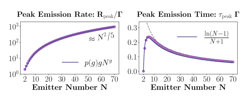
Figure 2: Dicke superradiance. Comparison of Eq. 5 and Eq. 6 (dots) with the exact numerics based on the quantum master equation (continuous lines) as a function of $N$. (a) The exact value of the peak emission rate shows excellent agreement with Eq. 5, where $g=2-2/N$. The peak emission rate converges to $\Gamma N^{2}/5$ for large $N$. (b) The peak emission time, and also shown is the time $\tau_{d}=\ln N/(\Gamma N)$ [2] (gray dashed line).

III Superradiance Process

We assume that the system is in initially in the product state $|\psi_{0}\rangle=\bigotimes_{n=1}^{N}|e_{n}\rangle$ with its time evolution governed by Eq. II. If the decay process is superradiant (see Table 1), the emission peak will occur at a delayed time $t>0$, as opposed to exponential or weakly correlated decay, where the maximum emission occurs at $t=0$. To find the peak emission rate and time means tracking the dissipative time dynamics and solving the superradiant decay problem with the emitter density operator $\rho$.

The key result of this work is the following observation: The peak emission rates $R_{\mathrm{peak}}$ shown in Fig. 2(b) depend strongly on the microscopic details of the emitter ensemble, such as geometry, density, type of emitter, dipole orientation. However, upon normalization by $gN^{g}$, we find in Fig. 2(c) that the peak emission rates of any emitter ensemble configuration and emitter type follow the same curve as a function of the second-order correlation function $g^{(2)}(0)$, in Eq. 3. By introducing the short-hand notation $g\equiv g^{(2)}(0)$, the estimation for the peak emission rate reads

$$R_{\mathrm{peak}}=\Gamma\ p(g)\ g\ N^{g},$$ (5)

if $g>1$ and $R_{\mathrm{peak}}=\Gamma N$ otherwise. The values of g are confined in the interval $(0,2)$ and superradiant decay occurs only for $g\in(1,2)$ [42]. The normalized emission rates shown in Fig. 1(c) follow the function $p(g)$, with the obvious value $p(1)=1$. Whether $p(g)$ is related to known mathematical functions, series, or polynomials warrants further studies and we find $p(g)$ by interpolating values extracted from exact numerical data based on quantum master equation simulations applied to various quantum emitter ensembles with details presented in Appendix A. However, in the regime $1.75\lesssim g<2$ we find that it becomes linear, $p(g)\approx-g/2+11/10$, while for $1\leq g\lesssim 1.75$ it is approximately given by $p(g)\approx\mathrm{exp}[-2(g-1)]$.

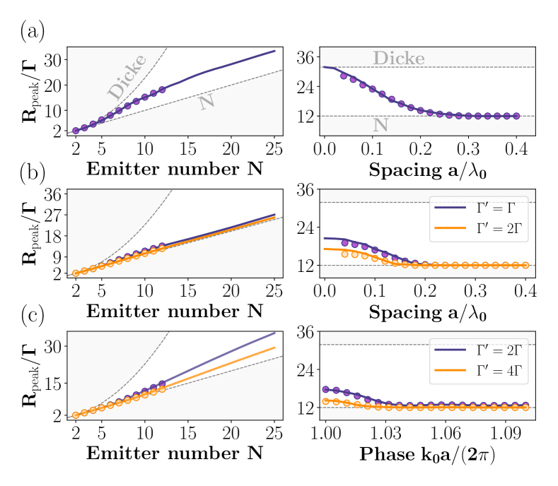
Figure 3: Superradiance peak emission rate as a function of emitter separation or number calculated via the quantum master equation (dots) and Eq. 5 (continuous lines). (a) Free-space emitters in a ring configuration, with $a=0.1\lambda_{0}$ on the left and in a $3\times 4$ array on the right. (b) Molecular emitters with the same geometry as in (a) with $a=0.1\lambda_{0}$ on the left and non-collective rates $\Gamma^{\prime}=\Gamma$ (blue) and $\Gamma^{\prime}=2\Gamma$ (orange). (c) Emitter chain coupled to a single-mode waveguide with $k_{0}a=0.02\pi$ on the left and $N=12$ on the right as well as decay rates $\Gamma^{\prime}=2\Gamma$ (blue) and $\Gamma^{\prime}=4\Gamma$ (orange) into non-guided modes. In plots (a) and (b) the emitters are circularly polarized in the array plane. The quantum master equation simulations in Eq. II inlcude the Hamiltonian, but in Eq. 5 it is not accounted for. The influence of the Hamiltonian is treated in Appendix D.

The time of peak emission has been studied in the limit of Dicke superradiance and is historically called ”delay time” [48, 2], since peak emission occurs at a delayed time $t>0$. Here we present a formula that estimates the peak emission time for any kind of two-level emitter ensemble as

$$\tau_{\mathrm{peak}}=\frac{1}{\Gamma}\frac{\ln\Big{(}\mathrm{Var}\big{(}{\{\Gamma_{k}\}/\Gamma}\big{)}-\Gamma^{\prime}/\Gamma\Big{)}}{\Big{(}\mathrm{Var}\big{(}{\{\Gamma_{k}\}/\Gamma}\big{)}+5\Gamma^{\prime}/\Gamma+2\Big{)}}\ ,$$ (6)

if $\mathrm{Var}\big{(}{\{\Gamma_{k}\}/\Gamma}\big{)}>1+\Gamma^{\prime}/\Gamma$ and $\tau_{\mathrm{peak}}=0$ otherwise. Below we apply these formulas to specific systems, namely Dicke superradiance, atomic emitter arrays in free space, molecular ensembles, and emitters coupled to a single-mode waveguide reservoir. The validity of these formulas is not reliant on the geometry of the emitter ensemble or other microscopic details, since the variance of the eigenvalues is general [42, 54].

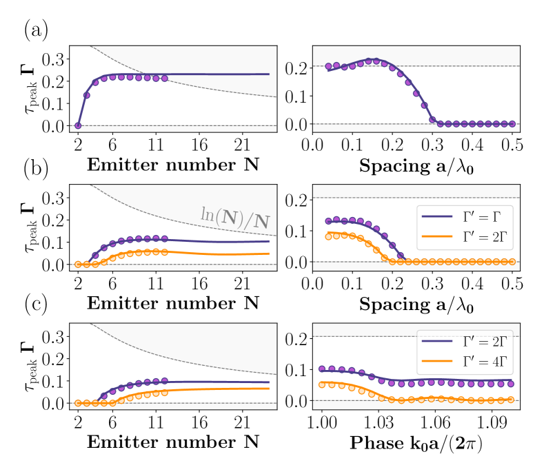
Figure 4: Time of peak emission as a function of emitter separation or number calculated via the quantum master equation (dots) and Eq. 6 (continuous lines) for the same parameters as in Fig. 3. (a) Free-space emitter ring, (b) Molecular emitters and (c) Emitter chain coupled to a single-mode waveguide reservoir. The upper gray dashed line indicates the time $\tau_{d}=\ln N/(N\Gamma)$ [2, 48].

Dicke superradiance – The paradigmatic example studied by Dicke [1] of $N$ indistinguishable two-level emitters, leads to $\Gamma_{nm}=\Gamma$ for all $n,m$ and furthermore we assume $\Gamma^{\prime}=0$. Under these conditions, Eq. 3 simplifies to $g=2-2/N$ and using Eq. 5, the peak emission rate for $N\geq 8$ is approximately given by

$$R_{\mathrm{peak}} \approx\frac{\Gamma}{5}\ \Big{(}1+\frac{10}{N}\Big{)}\ \Big{(}1-\frac{1}{N}\Big{)}\ N^{\big{(}2-\frac{2}{N}\big{)}},$$ (7)

using $p(2-2/N)\approx 11/10-g/2$ for $g\gtrsim 1.75$ (see Appendix A) and converges to $\Gamma N^{2}/5$ for large $N$, shown in Fig. 2(a). Eq. 4 results in $\mathrm{Var}({\{\Gamma_{k}\}/\Gamma})=N-1$ and thus in a peak emission time $\Gamma\tau_{\mathrm{peak}}=\ln(N-1)/(N+1)$, close to the delay time $\ln N/(\Gamma N)$ presented in Ref. [2]. Both show excellent agreement in Fig. 2(b) with exact numerics for the large $N$ limit, while the expression obtained here also agrees well at small $N$. We remark, that for emitters with non-collective decay, Dicke superradiance occurs only for $N-2>\Gamma^{\prime}/\Gamma$ [55].

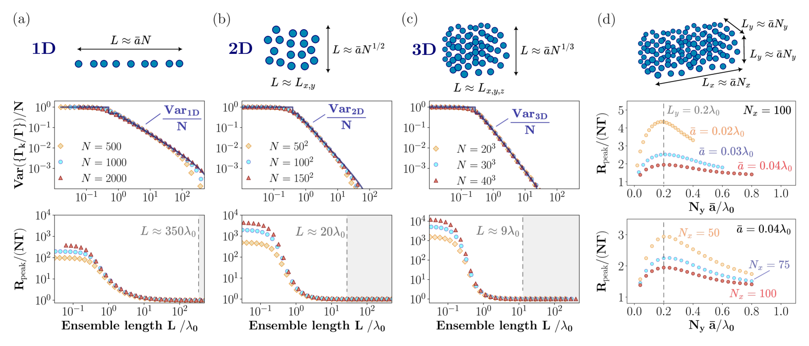
Figure 5: Universal length scaling and bound for free-space superradiance in (a) chain, (b) square and (c) cubic ensembles of two-level emitters. The variance in Eq. 4 determines the exponent $g$ for superradiant peak emission in Eq. 5 and exhibits a universal dependence on the length scale $L=\bar{a}N^{1/\mathcal{D}}$, where $\mathcal{D}$ is the ensemble dimension and $\bar{a}$ is the average emitter spacing. The average spacing is obtained by initializing perfect lattices with lattice spacings $a$ and randomly disorder emitter positions according to a normal distribution of standard deviation $\sigma/a=2$ (see Appendix C). All plots are shown as a function of the spacing $a/\lambda_{0}=[10^{-4},10^{1}]$ and in (d) as a function of the emitter number $N_{y}=1,...,20$. The gray regions indicate the ensemble lengths with $\mathrm{Var(\{\Gamma_{k}\}/\Gamma)/N}\leq 10^{-3}$, where the superradiant peak emission reduces to $R_{\mathrm{peak}}\approx N\Gamma$. (d) For elongated ensembles we find maximal superradiant enhancement for a side length of $L_{y}\approx 0.2\lambda_{0}$ irrespective of emitter number or spacing. Dipole orientations are $\mathbf{d}=(0,0,1)$ in all plots, however, the same conclusions and qualitatively similar curves are obtained considering other dipole orientations in the limit of large $N$. Bounds on the ensemble lengths and expressions for the variances $\mathrm{Var}_{\mathrm{1D,2D,3D}}$ are shown in Table 2.

Emitter ensembles in free-space – Quantum emitter ensembles in free-space decay collectively and superradiantly when their average nearest-neighbor separation is small enough, where the minimal spacing generally depends on the dimensionality of the ensemble [42, 54]. Here we assume identical quantum emitters with $\Gamma^{\prime}=0$ in various ordered configurations, however, the results apply equally to disordered ensembles, presented below and in Appendix C. In Fig. 3(a) peak emission rates are shown for ring, chain, and 2D square geometries, as a function of emitter number and spacing. The exact numerics (dots) based on the quantum master equation in Eq. II show good agreement with Eq. 5. At small spacings, $a\lesssim 0.05\lambda_{0}$ deviations appear, due to the influence of the Hamiltonian in the decay dynamics (see Appendix D). The corresponding peak emission times are plotted in Fig. 4(a) with the same parameters.

Molecular and solid-state emitters – Molecular or solid-state emitters in the excited electronic state decay both collectively ($\Gamma$) via the zero-phonon line (ZPL) and a manifold of vibrational, rotational or phononic states with a total rate quantified by $\Gamma^{\prime}$ and illustrated in Fig. 1(a) [33]. This leads to a quantum efficiency (QE) of the emitter $\mathrm{QE}={\Gamma}/({\Gamma+\Gamma^{\prime}})$ which reduces Eq. 3 and thus leads to a reduced superradiant emission (Fig. 1(b)). However, this is counteracted by the ability to realize deeply subwavelength ensembles with molecular aggregates reaching spacing on the order of tens of nanometers [13, 14], creating the condition for large numbers of emitters to decay collectively. Fig. 3(b) and Fig. 4(b) show comparisons of peak emission rates and times between exact numerics for up to $N=12$ emitter with the quantum master equation. The non-collective rates are $\Gamma^{\prime}=1\Gamma$ and $\Gamma^{\prime}=2\Gamma$, corresponding to quantum efficiencies $QE=50\%$ and $QE\approx 33\%$ respectively. Similar values can be found for instance in Dibenzoterrylene (DBT) molecules embedded in organic nanocrystals [33].

Single-mode waveguide reservoir – Two-level quantum systems coupled to a single-mode (bidirectional) waveguide are illustrated in Fig. 1(a). The coupling efficiency $\beta$ is defined as the ratio of the radiative decay rate of an individual emitter into the waveguide mode $\Gamma$ to its total decay rate $\Gamma+\Gamma^{\prime}$, namely $\mathcal{\beta}={\Gamma}/({\Gamma+\Gamma^{\prime}})$ [53]. The system consists of a chain of emitters positioned along the waveguide at positions $\{x_{n}\}$. For clarity, we assume an ordered chain with nearest-neighbor separation $a$, while in Appendix C we present the case of ensembles with positional disorder. The variance in Eq. 4 now simplifies to [55]

$$\mathrm{Var}\bigg{(}\frac{\{\Gamma_{k}\}}{\Gamma}\bigg{)}=\frac{N-2}{2}+\frac{\sin^{2}(Nk_{\mathrm{0}}a)}{2N\sin^{2}(k_{\mathrm{0}}a)},$$ (8)

using the waveguide couplings presented in Appendix B, which depend on the relative phase $k_{\mathrm{0}}a$, with the wavenumber $k_{0}$ of the guided mode on resonance with the emitter.

Dimension	$\mathbf{\mathrm{\textbf{Var}}_{\mathrm{\textbf{1D,2D,3D}}}}$	Ensemble length
1D (chain)	$\displaystyle\frac{N}{\lceil 2N\bar{a}/\lambda_{0}\rceil}-1$	$L\lesssim 50\lambda_{0}$
2D (square)	$\displaystyle\frac{N}{\lceil 1.5N(\bar{a}/\lambda_{0})^{1.75}\rceil}-1$	$L\lesssim 5\lambda_{0}$
3D (cubic)	$\displaystyle\frac{N}{\lceil N(\bar{a}/\lambda_{0})^{2}/3\rceil}-1$	$L\lesssim 3\lambda_{0}$

Table 2: Linear chain, square, and cubic ensembles in free-space assuming an equal emitter number in each dimension and with average nearest-neighbor spacing $\bar{a}$. The variance can be approximated by a simple expression depending only on the average nearest-neighbor spacing $\bar{a}$ and total emitter number $N$. Here $\lceil x\rceil$ is the ceiling function and we add the condition $\lceil x\rceil=N$ if $x>N$ such that it is valid for all spacings. In Fig. 5 (a)-(c) we find excellent agreement with the exact numerical value of the variance. We define the maximum ensemble length $L$ as the value where $\mathrm{Var(\{\Gamma_{k}\}/\Gamma)/N}\sim 10^{-3}$, at which point $R_{\mathrm{peak}}\approx N\Gamma$ according to Eq. 3 and Eq. 4 (shown in Fig. 5). This sets an upper limit on the spatial extent of emitter ensembles with 3D dipole-dipole interactions, such as in free space.

Note, that the variance depends only on two parameters, the emitter number $N$ and spacing $a$, allowing us to estimate the peak emission rate and time for large $N$. In Fig. 3(c) and Fig. 4(c) we plot the comparison between exact numerics and the formulas in Eq. 5 and Eq. 6 for linear chains of emitters. Superradiant decay emerges in particular if the relative phase is close to integer multiples of $\pi$, the Dicke limit, as seen by the appearance of a finite delay time in Fig. 4(c). Lastly, as opposed to its free-space counterpart, the variance has a minimum value of $N/2-1$, namely the emitters always decay superradiantly if the condition $N/2>1+\Gamma^{\prime}/\Gamma$ is fulfilled.

We note, that the Hamiltonian $\mathcal{H}$ is not accounted for in Eq. 5 and Eq. 6 and generally leads to a reduction of peak emission at spacings $a<0.1\lambda_{0}$, however its influence decreases with emitter number as shown in the Supplement D.

IV Universal scalings and bounds

In this section, we show that superradiance in free space follows a universal length scaling and answer the question: what is the maximal spatial extent an emitter ensemble can reach while still being superradiant, namely $R_{\mathrm{peak}}\gtrsim N\Gamma$? Furthermore, we find simple expressions for the variance in Eq. 4, which require just two parameters, the average spacing $\bar{a}$ and total emitter number $N$.

In Fig. 5 (a)-(c) we assume ensembles of $N$ emitters with an equal number of emitters in each spatial dimension, resulting in an ensemble side length $L=\bar{a}N^{1/\mathcal{D}}$ and where $\mathcal{D}$ is the ensemble dimension. The average spacing is obtained by initializing perfect lattices with lattice spacings $a$ and randomly disorder the emitter positions according to a normal distribution with standard deviation $\sigma$. For all plots in Fig. 5 we choose $\sigma/a=2$, however in Appendix C we show, that the variance in Eq. 4 remains mostly unaffected for the even larger positional disorder. In (a)-(c) the variance exhibits the same scaling as a function of the ensemble length $L$ by varying the spacing, irrespective of the emitter number. We define the maximum ensemble length as the value where $\mathrm{Var(\{\Gamma_{k}\}/\Gamma)/N}\sim 10^{-3}$, at which point $R_{\mathrm{peak}}\approx N\Gamma$ according to Eq. 3 and Eq. 4. We also find numerically, that the variances can be well approximated by simple expressions which depend only on the spacing and emitter number, denoted as $\mathrm{Var}_{\mathrm{1D}}$, $\mathrm{Var}_{\mathrm{2D}}$ and $\mathrm{Var}_{\mathrm{3D}}$ in Fig. 5. Expressions are shown in Table 2 along with the bounds on the maximum ensemble lengths. In Fig. 5(d) we study the case of an elongated ensemble in 3D, where $L_{x}>L_{y}$ and find that a maximal superradiant enhancement is reached for $L_{y}\approx 0.2\lambda_{0}$ irrespective of the emitter spacing and length $L_{x}$. The dipole orientations in Fig. 5 are $\mathrm{d}=(0,0,1)^{T}$, however, we find qualitatively the same conclusions for different orientations and large $N$.

We note, that in 1D arrays the expression for the variance in Table 2 has an alternative interpretation. For ordered 1D lattices, the light line in the first Brillouin zone is located at $k_{0}a/\pi=2a/\lambda_{0}$, in the limit of large $N$ [57, 58]. As a consequence the number of radiant decay rates $(\Gamma_{k}\geq\Gamma)$ enclosed by the light line is given by $\lceil 2aN/\lambda_{0}\rceil$ [59], which appears in the denominator of the expression for the variance. Remarkably, we find numerically, that the expressions in Table 2 are valid even in the presence of position disorder, where $a$ corresponds to the average nearest-neighbor spacing, as shown in Fig. 5.

At closer inspection, one can observe the step function behavior as the variance reaches $\gtrsim 0.1$, which stems from the ceiling function used in Table 2. In 1D the interpretation is again connected with the number of radiant collective decay rates: As the ensemble approaches the Dicke limit the number of radiant collective decay rates ($\Gamma_{k}\geq\Gamma$) approaches small integer values until only a single rate $(N\Gamma)$ remains. The variance takes steps from $N/3-1$ to $N/2-1$ to $N-1$ as the number of radiant collective rates decreases from three to two to one. Evidently, in the limit of non-interacting emitters the number of radiant modes is given by $N$ and the variance is zero.

V Conclusions and outlook

We have provided compact and tractable analytical formulas for accurately estimating the peak emission rate and time for fully inverted two-level quantum emitters undergoing collective superradiant decay. Remarkably, these results are universally applicable, independent of specific microscopic details and the geometric configuration of the emitter ensemble—owing to their origin in the variance of the eigenvalues of the collective dissipation matrix. The results are supported through numerical comparisons with exact quantum master equation simulations for small emitter numbers. We also identified universal length scalings and derived bounds for superradiance in free space emitter ensembles with positional disorder. Further, we determined the optimal cross-sectional size for three-dimensional elongated emitter ensembles, such that superradiant enhancement is maximized.

This work addresses key questions in extended emitter ensembles undergoing superradiance, specifically the maximum spatial size of emitter ensembles that can support superradiant emission. Furthermore, for one-dimensional arrays, we established a direct connection between the variance of the eigenvalues of the collective dissipation matrix and the number of radiant modes contained within the light line. Although the formulas do not account for Hamiltonian dynamics and dephasing in the excited emitter state, their influence appears to become more negligible for increasing emitter numbers [42]. Future extensions could include more complex scenarios such as multi-level emitters, chiral waveguide environments, and partially excited initial states. Finally, the intriguing connection between the variance of collective decay rates and the light cone structure, warrants further investigation [57, 58].

Acknowledgments - R.H. and S.F.Y. acknowledge NSF via PHY-2207972, the CUA PFC PHY-2317134.

Appendix A The function $\boldsymbol{p(g)}$

$\boldsymbol{g}$	$\boldsymbol{p(g)}$
1.0	1.0
1.05	0.875
1.1	0.79
1.15	0.72
1.2	0.663
1.25	0.603

$\boldsymbol{g}$	$\boldsymbol{p(g)}$
1.3	0.554
1.35	0.5
1.4	0.45
1.45	0.41
1.5	0.368
1.55	0.335

$\boldsymbol{g}$	$\boldsymbol{p(g)}$
1.6	0.3
1.65	0.275
1.7	0.25
1.75	0.225
1.8	0.2
1.85	0.175

$\boldsymbol{g}$	$\boldsymbol{p(g)}$
1.9	0.15
1.95	0.125
1.992	0.104
2.0	0.1

Table 3: The $g$ values correspond to values of the second-order correlation $g^{(2)}(0)$ at $t=0$ in Eq. 3. Superradiance occurs only in the interval $1<g<2$ and the values of $p(g)$ are the corresponding normalized peak emission rates $p(g)=R_{\mathrm{peak}}/(\Gamma gN^{g})$ obtained from master equation simulations using multiple realizations of various quantum emitter ensembles $(N\leq 12)$ and averaging over the values (see Fig. 1(c) in the main text). This table of values can be interpolated to create the continuous function $p(g)$ in the interval $g\in[1,2]$ and in this work a simple linear interpolation is used.

In Fig. 6(a) the function $p(g)$ is plotted using the data points from Table 3, while in (b) a zoomed-in section is shown for $g\in[1.6,2)$ where $g=2-2/N$ and with $N=8\dots 250$.

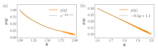
Figure 6: (a) The function $p(g)$ plotted for $g\in[1,2]$ using a linear interpolation of the data in Table 3 with orange dots representing the normalized peak emission rates in the Dicke limit, $R_{\mathrm{peak}}/(\Gamma gN^{g})$, obtained from the quantum master equation. For $g\in[1,1.75]$ the function $p(g)$ can be approximated by $e^{-2(g-1)}$. (b) A close up for $g\in[1.6,2]$ shows a linear dependence approximated by $p(g)=-0.5g+1.1$.

Fig. 6 shows, that the function $p(g)$ can be approximated by

$$p(g)=\begin{cases}\approx\mathrm{e}^{-2(g-1)}&\text{if $1\leq g\lesssim 1.75$}\\ \approx-\frac{1}{2}g+\frac{11}{10}&\text{if $1.75\lesssim g\leq 2$}\end{cases}$$ (9)

Since the function $p(g)$ becomes linear in $g$ for $g\gtrsim 1.75$ or in the Dicke limit for $N\geq 8$, it is possible to approximate the peak emission rate for Dicke superradiance as

$$R_{\mathrm{peak}}/\Gamma\approx\Big{(}\frac{11}{10}-\frac{g}{2}\Big{)}gN^{g} =\Big{(}\frac{11}{10}-\frac{g}{2}\Big{)}\Big{(}2-\frac{2}{N}\Big{)}N^{2-2/N}=\frac{1}{5}\Big{(}1-\frac{11}{N}+\frac{10}{N^{2}}\Big{)}N^{2-2/N},$$

which converges to $\Gamma N^{2}/5$ for large $N$, the upper bound for the total emission rate of a fully inverted two-level quantum emitter ensemble.

Appendix B Quantum master equation and dipole-dipole interactions

The system consists of $N$ two-level emitters with resonance frequency $\omega$, decay rate $\Gamma=\omega^{3}\mu^{2}/(3\pi c^{3}\epsilon_{0}\hbar)$ and non-collective decay rate $\Gamma^{\prime}$. By tracing out the electromagnetic field using the Born-Markov approximation [60], the emitter density matrix $\rho$ evolves in time as

$$\dot{\rho}=-\frac{i}{\hbar}[\mathcal{H},\rho]+\sum_{n,m=1}^{N}\Gamma_{nm}\Big{(}\sigma_{n}\rho\sigma_{m}^{\dagger}-\frac{1}{2}\{\sigma^{\dagger}_{n}\sigma_{m},\rho\}\Big{)}+\sum_{n=1}^{N}\Gamma^{\prime}\Big{(}\sigma_{n}\rho\sigma_{n}^{\dagger}-\frac{1}{2}\{\sigma^{\dagger}_{n}\sigma_{n},\rho\}\Big{)},$$ (10)

where $\sigma_{n}=|g_{n}\rangle\langle e_{n}|$ is the spin lowering operator for the $n^{th}$ emitter and the Hamiltonian in the rotating frame of the emitter frequency $\omega$ is given by

$$\mathcal{H}=\sum_{n,m\neq n}^{N}J_{nm}\sigma^{\dagger}_{n}\sigma_{m},$$ (11)

which results in coherent exchange of excitations reducing the peak emission rate at small spacings, where the coherent exchange rate becomes large, as shown in Fig. 10 and Fig. 11. We note, that the second term in Eq. 10 can be written in diagonal form as

$$\mathcal{L}[\rho]=\sum_{k=1}^{N}\Gamma_{k}\Big{(}\mathcal{O}_{k}\rho\mathcal{O}_{k}^{\dagger}-\frac{1}{2}\{\mathcal{O}_{k}^{\dagger}\mathcal{O}_{k},\rho\}\Big{)},$$ (12)

where $\Gamma_{k}$ are the eigenvalues of the $N\times N$ dissipation matrix with elements $\Gamma_{mn}$ and $\mathcal{O}_{k}$ are the associated collective jump operators given by $\mathcal{O}_{k}=\sum_{n=1}^{N}c_{k,n}\sigma_{n}$ with coefficients $c_{k,n}$ fulfilling $\sum_{k=1}^{N}\Gamma_{k}|c_{k,n}|^{2}=\Gamma$ and $\sum_{n=1}^{N}c^{*}_{k,n}c_{k^{\prime},n}=\delta_{kk^{\prime}}$. The coherent and dissipative dipole-dipole couplings between emitters $n$ and $m$ read

$$J_{nm}-\frac{i\Gamma_{nm}}{2}=-\frac{3\pi\Gamma}{\omega_{0}}\mathbf{d}^{\dagger}\cdot\mathbf{G}(\mathbf{r}_{nm},\omega_{0})\cdot\mathbf{d},$$ (13)

where $\mathbf{d}$ is the transition dipole moment matrix element, $\mathbf{r}_{nm}=\mathbf{r}_{n}-\mathbf{r}_{m}$ is the connecting vector between emitters $n$ and $m$. The Green’s tensor $\mathbf{G}(\mathbf{r}_{nm},\omega_{0})$ is the propagator of the electromagnetic field between emitter positions $\boldsymbol{r}_{n}$ and $\boldsymbol{r}_{m}$, and reads for 3D dipole-dipole interactions

$$\mathbf{G}(\mathbf{r}_{nm},\omega_{0})=\frac{e^{ik_{0}r_{nm}}}{4\pi k_{0}^{2}r_{nm}^{3}}\bigg{[}\left(k_{0}^{2}r_{nm}^{2}+ik_{0}r_{nm}-1\right)\mathbb{1}+\left(-k_{0}^{2}r_{nm}^{2}-3ik_{0}r_{nm}+3\right)\frac{\mathbf{r}_{nm}\otimes\mathbf{r}_{nm}}{r_{nm}^{2}}\bigg{]},$$ (14)

with $r_{nm}=|\mathbf{r}_{nm}|$ and $k_{0}=2\pi/\lambda_{0}$, where $\lambda_{0}$ is the wavelength of light emitted by the emitters. Meanwhile, for one-dimensional dipole-dipole interactions in a single-mode waveguide, the couplings simplify to [53]

$$J_{nm}-\frac{i\Gamma_{nm}}{2}=-\frac{i\Gamma}{2}\ \mathrm{exp}\Big{(}ik_{\mathrm{0}}|{x_{n}}-x_{m}|\Big{)},$$ (15)

which exhibits an infinite range, periodic modulation with $k_{0}=\omega_{0}/c$ being the wavevector of the guided mode on resonance with the emitters, and it is assumed that the emitters are positioned at $\{x_{n}\}$ along the waveguide.

The variance is now written for a waveguide reservoir as [55]

$$\mathrm{Var}\bigg{(}\frac{\{\Gamma_{k}\}}{\Gamma}\bigg{)}=\sum_{k=1}^{N}\frac{\Gamma_{k}^{2}}{N\Gamma^{2}}-1=2N-1+\frac{2}{N}\Bigg{[}\Big{(}\sum_{n=1}^{N}\cos(2k_{\mathrm{0}}x_{n})\Big{)}^{2}+\Big{(}\sum_{n=1}^{N}\sin(2k_{\mathrm{0}}x_{n})\Big{)}^{2}\Bigg{]},$$ (16)

where for simplicity we assume identical dissipative coupling rates $\Gamma_{n}=\Gamma$ into the waveguide mode for all emitters. For linear chains with equidistant spacing $a$, it simplifies to

$$\mathrm{Var}\bigg{(}\frac{\{\Gamma_{k}\}}{\Gamma}\bigg{)}=\frac{N-2}{2}+\frac{\sin^{2}(Nk_{\mathrm{0}}a)}{2N\sin^{2}(k_{\mathrm{0}}a)}.$$ (17)

Appendix C Positional disorder

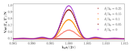
Figure 7: Positional disorder for a single-mode waveguide reservoir. $N=100$ emitters are positioned along the waveguide at positions $\{x_{n}\}$ with waveguide wavenumber $k_{0}=2\pi$, randomly disordered according to a Gaussian distribution with standard deviation $\delta$ around $\{x_{n}\}$ and averaged over $100$ samples. The dots represent the averaged values of Eq. 16 and the continuous lines correspond to Eq. 18. We find excellent agreement for all disorder values and note that $\delta/\lambda_{0}=0.25$ corresponds to a completely disordered ensemble as the waveguide couplings in Eq. 15 can now take any value between $0$ and $\Gamma$.

We find numerically, that in the presence of positional disorder of the emitters, $x_{n}+\lambda_{0}\epsilon_{n}$, where $\epsilon_{n}$ is a random displacement with standard deviation $\delta$, expression Eq. 17 can be written as

$$\mathrm{Var}\bigg{(}\frac{\{\Gamma_{k}\}}{\Gamma}\bigg{)}\approx\frac{N-2}{2}+\sqrt{\cos^{3}(2\pi\delta)}\frac{\sin^{2}(Nk_{\mathrm{0}}a)}{2N\sin^{2}(k_{\mathrm{0}}a)}.$$ (18)

Fig. 7 shows excellent agreement between Eq. 18 and the exact values obtained from Eq. 16 for increasing positional disorder strengths. We notice that the variance decreases with position disorder as opposed to the free-space case shown in the main text. In particular for $\delta=0.25\lambda_{0}n$, where $n=1,2,3...$, the system is maximally disordered, reducing the variance to the minimum value $(N-2)/2$, which still allows for superradiant decay if the condition $N-2>\Gamma^{\prime}/\Gamma$ is fulfilled. Assuming $\Gamma^{\prime}=0$, the peak emission time is then given by $\tau_{peak}\Gamma=\ln(N/2-1)/(N/2+1)$ and $g=3/2-1/N$ converges to $3/2$ for large $N$, which leads to $R_{\mathrm{peak}}/\Gamma\approx 0.55N^{3/2}$ for a completely disordered chain of $N$ two-level emitters coupled to a single-mode waveguide.

In Fig. 9 (a)-(c) we show the influence of positional disorder on the variance $\mathrm{Var(\{\Gamma_{k}\}/\Gamma)/N}$ for 1D,2D and 3D ensembles in free space.

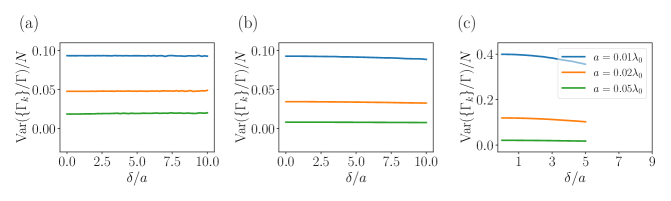
Figure 8: Positional disorder in free-space ensembles. (a) Chain of $N=500$ emitters. (b) Square array with $N=150\times 150$ emitters. (c) Cubic array with $N=30\times 30\times 30$ emitters. The emitters are randomly disordered around the initial position according to a normal distribution with standard deviation $\delta$. The curves are produced by single random realizations and the dipole orientations are $\mathbf{d}=(0,0,1)^{T}$ in all plots.

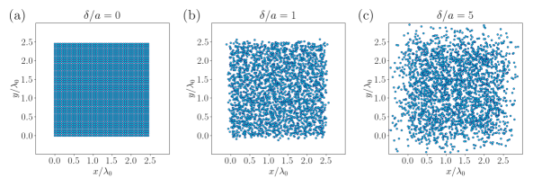
Figure 9: Positional disorder in free-space ensembles. The emitter positions are plotted for a square array with $N=50\times 50$ emitters and spacing $a=0.05\lambda_{0}$ for (a) $\sigma/a=0$, (b) $\sigma/a=1$, (c) $\sigma/a=5$.

Appendix D Influence of the Hamiltonian on superradiant decay

In Fig. 10 the influence of the Hamiltonian dynamics in Eq. 10 on the peak emission properties is plotted for a ring of emitters in free space and a waveguide reservoir in Fig. 11. The emitters are initially fully excited and decay either with or without the Hamiltonian term present in Eq. B. For smaller emitter spacings in Fig. 10 the difference is more pronounced as the coherent dipole-dipole shifts $J_{nm}$ become substantial and dephases the emission process away from the symmetric Dicke states, while for the peak time a difference arises only in the interval $a\in(0.05,0.15)$. For the waveguide, the Hamiltonian influence increases for $k_{0}a\neq 0$, where the shifts become more pronounced as they depend on the sine of the relative phase. How to accurately quantify the influence of the Hamiltonian on the correlated decay and peak emission properties is an open question at this point and has to be investigated further.

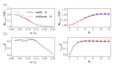
Figure 10: Free-space simulation using the quantum master equation. Influence of the Hamiltonian on the peak emission rate and time for an emitter ring with the emitters being circularly polarized in the plane. (a) The peak emission rate as a function of spacing for $N=10$ (left) and as a function of $N$ for $a=0.1\lambda_{0}$ on the right. (b) The peak emission time with the same parameters as in (a).

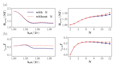
Figure 11: Waveguide simulation using the quantum master equation. Influence of the Hamiltonian on the peak emission rate and time for an emitter chain with equidistant spacings, coupled to a one-dimensional waveguide reservoir. (a) The peak emission rate as a function of the relative phase $k_{0}a$ for $N=10$ (left) and as a function of $N$ for $k_{0}a=0.08\pi$ on the right. (b) The peak emission time with the same parameters as in (a).

Appendix E Partially excited ensemble in the Dicke limit

A partially excited ensemble of two-level emitters can be written as

$$|\psi\rangle_{\varphi}=\bigotimes_{n=1}^{N}\Big{(}\sqrt{1-\varphi}|g_{n}\rangle+\sqrt{\varphi}|e_{n}\rangle\Big{)}=\sum_{m=1}^{N}\varphi^{m/2}(1-\varphi)^{(N-m)/2}\frac{(S^{\dagger})^{m}}{m!}\bigotimes_{n=1}^{N}|g_{n}\rangle,$$ (19)

where we assume no relative phase between the emitters, that is, a symmetric excitation and $\varphi\in[0,1]$. The initial state is now given by a binomial distribution of symmetric Dicke states $|m\rangle\propto(S^{\dagger})^{m}|g_{n}\rangle^{\otimes n}$. The total excitation number at $t=0$ is now given by $\varphi N$ and the total photon emission at $t=0$ reads

$$R_{\varphi}(0)/\Gamma=N\varphi^{2}+N^{2}\varphi(1-\varphi).$$ (20)

The initial emission is maximal for $\varphi=N/\big{(}2(N-1)\big{)}$ and leads to $\mathrm{Max}\{R_{\varphi}(0)/\Gamma\}=N^{3}/\big{(}4(N-1)\big{)}$. In the limit of large $N$ this approaches $\approx\Gamma N^{2}/4$. Note, that the maximal emission rate from a pure Dicke state state occurs for $m=N/2$ (or $m=(N\pm 1)/2$ for $N$ odd), namely at half-excitation and is given by $\Gamma N/2(N/2+1)$.

Similarly, the second-order correlation function at $t=0$ can be evaluated as

$$g^{(2)}(0)_{\varphi}=\frac{\Gamma^{2}\langle\psi_{\varphi}|S^{\dagger}S^{\dagger}SS|\psi_{\varphi}\rangle}{R_{\varphi}(0)^{2}}=\frac{\Gamma^{2}}{R_{\varphi}(0)^{2}}\Big{(}\sum_{m=2}^{N}\varphi^{m}(1-\varphi)^{(N-m)}\binom{N}{m}h_{m}h_{m-1}\Big{)},$$ (21)

where $h_{m}=m(N-m+1)$ are the coefficients resulting from the action of $S$ on the Dicke states, $S|m\rangle=\sqrt{h_{m}}|m-1\rangle$ and $S^{\dagger}|m\rangle=\sqrt{h_{m+1}}|m+1\rangle$. For the fully excited case with $h_{N}=N$, $h_{N-1}=2(N-1)$, $\varphi=1$ and $R_{\varphi}(0)=N$ we recover again

$$g^{(2)}(0)=\frac{\Gamma^{2}}{\Gamma^{2}N^{2}}\Big{(}2N(N-1)\Big{)}=2-\frac{2}{N}.$$ (22)

We proceed by again writing the superradiance criterion as $g^{(2)}(0)>1$, which is now defined with respect to $R_{\varphi}(0)$ and not $N\Gamma$ as in the fully excited case. As an example, for $\varphi=N/\big{(}2(N-1)\big{)}$ the ensemble is (maximally) superradiant at $t=0$ but will not exhibit a superradiant peak at a later time and indeed we obtain $g^{(2)}(0)_{\varphi}<1$.

References

- Dicke [1954] R. H. Dicke, Coherence in spontaneous radiation processes, Phys. Rev. 93, 99 (1954).
- Gross and Haroche [1982] M. Gross and S. Haroche, Superradiance: An essay on the theory of collective spontaneous emission, Physics Reports 93, 301 (1982).
- Anatolii V Andreev et al. [1980] Anatolii V Andreev, Vladimir I Emel’yanov, and Yu A Il’inskiĭ, Collective spontaneous emission (dicke superradiance), Soviet Physics Uspekhi 23, 493 (1980).
- Haake and Glauber [1972] F. Haake and R. J. Glauber, Quantum statistics of superradiant pulses, Phys. Rev. A 5, 1457 (1972).
- Lin and Yelin [2012] G.-D. Lin and S. F. Yelin, Superradiance in spin- particles: Effects of multiple levels, Phys. Rev. A 85, 033831 (2012).
- Rehler and Eberly [1971] N. E. Rehler and J. H. Eberly, Superradiance, Phys. Rev. A 3, 1735 (1971).
- Benedict et al. [1996] M. Benedict, A. Ermolaev, V. Malyshev, I. Sokolov, and E. Trifonov, Super-radiance: Multiatomic Coherent Emission (1996).
- Haake et al. [1993] F. Haake, M. I. Kolobov, C. Fabre, E. Giacobino, and S. Reynaud, Superradiant laser, Physical review letters 71, 995 (1993).
- Meiser et al. [2009] D. Meiser, J. Ye, D. Carlson, and M. Holland, Prospects for a millihertz-linewidth laser, Physical review letters 102, 163601 (2009).
- Bohnet et al. [2012] J. G. Bohnet, Z. Chen, J. M. Weiner, D. Meiser, M. J. Holland, and J. K. Thompson, A steady-state superradiant laser with less than one intracavity photon, Nature 484, 78 (2012).
- Kocharovsky et al. [2017] V. V. Kocharovsky, V. V. Zheleznyakov, E. R. Kocharovskaya, and V. V. Kocharovsky, Superradiance: the principles of generation and implementation in lasers, Physics-Uspekhi 60, 345 (2017).
- Babcock et al. [2024] N. S. Babcock, G. Montes-Cabrera, K. E. Oberhofer, M. Chergui, G. L. Celardo, and P. Kurian, Ultraviolet superradiance from mega-networks of tryptophan in biological architectures, The Journal of Physical Chemistry B 128, 4035 (2024).
- Monshouwer et al. [1997] R. Monshouwer, M. Abrahamsson, F. van Mourik, and R. van Grondelle, Superradiance and exciton delocalization in bacterial photosynthetic light-harvesting systems, The Journal of Physical Chemistry B 101, 7241 (1997).
- Doria et al. [2018] S. Doria, T. S. Sinclair, N. D. Klein, D. I. G. Bennett, C. Chuang, F. S. Freyria, C. P. Steiner, P. Foggi, K. A. Nelson, J. Cao, A. Aspuru-Guzik, S. Lloyd, J. R. Caram, and M. G. Bawendi, Photochemical control of exciton superradiance in light-harvesting nanotubes, ACS Nano 12, 4556 (2018).
- Houde et al. [2018] M. Houde, A. Mathews, and F. Rajabi, Explaining fast radio bursts through dicke’s superradiance, Monthly Notices of the Royal Astronomical Society 475, 514 (2018).
- Zhang [2023] B. Zhang, The physics of fast radio bursts, Rev. Mod. Phys. 95, 035005 (2023).
- Bassani and et al. [2024] C. L. Bassani and et al., Nanocrystal assemblies: Current advances and open problems, ACS Nano 18, 14791 (2024).
- Cong et al. [2016] K. Cong, Q. Zhang, Y. Wang, G. T. Noe, A. Belyanin, and J. Kono, Dicke superradiance in solids, Journal of the Optical Society of America B 33, C80 (2016).
- Lemberger and Yavuz [2017] B. Lemberger and D. Yavuz, Effect of correlated decay on fault-tolerant quantum computation, Physical Review A 96, 062337 (2017).
- Yavuz [2014] D. D. Yavuz, Superradiance as a source of collective decoherence in quantum computers, Journal of the Optical Society of America B 31, 2665 (2014).
- Wang et al. [2007] T. Wang, S. F. Yelin, R. Côté, E. E. Eyler, S. M. Farooqi, P. L. Gould, M. Koštrun, D. Tong, and D. Vrinceanu, Superradiance in ultracold rydberg gases, Phys. Rev. A 75, 033802 (2007).
- Grimes et al. [2017] D. D. Grimes, S. L. Coy, T. J. Barnum, Y. Zhou, S. F. Yelin, and R. W. Field, Direct single-shot observation of millimeter-wave superradiance in rydberg-rydberg transitions, Phys. Rev. A 95, 043818 (2017).
- Kaluzny et al. [1983] Y. Kaluzny, P. Goy, M. Gross, J. M. Raimond, and S. Haroche, Observation of self-induced rabi oscillations in two-level atoms excited inside a resonant cavity: The ringing regime of superradiance, Phys. Rev. Lett. 51, 1175 (1983).
- Araújo et al. [2016] M. O. Araújo, I. Krešić, R. Kaiser, and W. Guerin, Superradiance in a large and dilute cloud of cold atoms in the linear-optics regime, Phys. Rev. Lett. 117, 073002 (2016).
- Chen et al. [2018] L. Chen, P. Wang, Z. Meng, L. Huang, H. Cai, D.-W. Wang, S.-Y. Zhu, and J. Zhang, Experimental observation of one-dimensional superradiance lattices in ultracold atoms, Phys. Rev. Lett. 120, 193601 (2018).
- Ferioli et al. [2021] G. Ferioli, A. Glicenstein, F. Robicheaux, R. T. Sutherland, A. Browaeys, and I. Ferrier-Barbut, Laser-driven superradiant ensembles of two-level atoms near dicke regime, Phys. Rev. Lett. 127, 243602 (2021).
- Goban et al. [2015] A. Goban, C.-L. Hung, J. D. Hood, S.-P. Yu, J. A. Muniz, O. Painter, and H. J. Kimble, Superradiance for atoms trapped along a photonic crystal waveguide, Phys. Rev. Lett. 115, 063601 (2015).
- Scheibner et al. [2007] M. Scheibner, T. Schmidt, L. Worschech, A. Forchel, G. Bacher, T. Passow, and D. Hommel, Superradiance of quantum dots, Nature Physics 3, 106 (2007).
- Rainò et al. [2018] G. Rainò, M. A. Becker, M. I. Bodnarchuk, R. F. Mahrt, M. V. Kovalenko, and T. Stöferle, Superfluorescence from lead halide perovskite quantum dot superlattices, Nature 563, 671 (2018).
- Bradac et al. [2017] C. Bradac, M. T. Johnsson, M. v. Breugel, B. Q. Baragiola, R. Martin, M. L. Juan, G. K. Brennen, and T. Volz, Room-temperature spontaneous superradiance from single diamond nanocrystals, Nature Communications 8, 1205 (2017).
- Haider et al. [2021] G. Haider, K. Sampathkumar, T. Verhagen, L. Nádvorník, F. J. Sonia, V. Valeš, J. Sýkora, P. Kapusta, P. Němec, M. Hof, O. Frank, Y.-F. Chen, J. Vejpravová, and M. Kalbáč, Superradiant emission from coherent excitons in van der waals heterostructures, Advanced Functional Materials 31, 2102196 (2021).
- Tiranov et al. [2023] A. Tiranov, V. Angelopoulou, C. J. van Diepen, B. Schrinski, O. A. D. Sandberg, Y. Wang, L. Midolo, S. Scholz, A. D. Wieck, A. Ludwig, A. S. Sørensen, and P. Lodahl, Collective super- and subradiant dynamics between distant optical quantum emitters, Science 379, 389 (2023).
- Lange et al. [2024] C. M. Lange, E. Daggett, V. Walther, L. Huang, and J. D. Hood, Superradiant and subradiant states in lifetime-limited organic molecules through laser-induced tuning, Nature Physics 20, 836–842 (2024).
- Kim et al. [2023] D. Kim, S. Lee, J. Park, J. Lee, H. C. Choi, K. Kim, and S. Ryu, In-plane and out-of-plane excitonic coupling in 2d molecular crystals, Nature Communications 14, 2736 (2023).
- Chumakov and et al. [2018] A. I. Chumakov and et al., Superradiance of an ensemble of nuclei excited by a free electron laser, Nature Physics 14, 261 (2018).
- Liedl et al. [2024] C. Liedl, F. Tebbenjohanns, C. Bach, S. Pucher, A. Rauschenbeutel, and P. Schneeweiss, Observation of superradiant bursts in a cascaded quantum system, Phys. Rev. X 14, 011020 (2024).
- Carmichael and Kim [2000a] H. Carmichael and K. Kim, A quantum trajectory unraveling of the superradiance master equation, Optics Communications 179, 417 (2000a).
- Mølmer et al. [1993] K. Mølmer, Y. Castin, and J. Dalibard, Monte carlo wave-function method in quantum optics, J. Opt. Soc. Am. B 10, 524 (1993).
- Dum et al. [1992] R. Dum, P. Zoller, and H. Ritsch, Monte carlo simulation of the atomic master equation for spontaneous emission, Phys. Rev. A 45, 4879 (1992).
- Holzinger et al. [2025] R. Holzinger, N. S. Bassler, J. Lyne, F. G. Jimenez, J. T. Gohsrich, and C. Genes, Solving dicke superradiance analytically: A compendium of methods (2025), arXiv:2503.10463 [quant-ph] .
- Holzinger and Genes [2025] R. Holzinger and C. Genes, An exact analytical solution for dicke superradiance (2025), arXiv:2409.19040 [quant-ph] .
- Masson and Asenjo-Garcia [2022] S. J. Masson and A. Asenjo-Garcia, Universality of dicke superradiance in arrays of quantum emitters, Nature Communications 13, 2285 (2022).
- Robicheaux [2021] F. Robicheaux, Theoretical study of early-time superradiance for atom clouds and arrays, Phys. Rev. A 104, 063706 (2021).
- Kubo [1962] R. Kubo, Generalized cumulant expansion method, Journal of the Physical Society of Japan 17, 1100 (1962), https://doi.org/10.1143/JPSJ.17.1100 .
- Rubies-Bigorda et al. [2023] O. Rubies-Bigorda, S. Ostermann, and S. F. Yelin, Characterizing superradiant dynamics in atomic arrays via a cumulant expansion approach, Phys. Rev. Res. 5, 013091 (2023).
- Mink and Fleischhauer [2023] C. D. Mink and M. Fleischhauer, Collective radiative interactions in the discrete truncated wigner approximation, SciPost Physics 15, 10.21468/scipostphys.15.6.233 (2023).
- Shammah et al. [2018] N. Shammah, S. Ahmed, N. Lambert, S. De Liberato, and F. Nori, Open quantum systems with local and collective incoherent processes: Efficient numerical simulations using permutational invariance, Phys. Rev. A 98, 063815 (2018).
- Haake et al. [1980] F. Haake, J. Haus, H. King, G. Schröder, and R. Glauber, Delay-time statistics and inhomogeneous line broadening in superfluorescence, Physical Review Letters 45, 558 (1980).
- Lehmberg [1970a] R. H. Lehmberg, Radiation from an -atom system. i. general formalism, Phys. Rev. A 2, 883 (1970a).
- Clemens et al. [2003] J. P. Clemens, L. Horvath, B. C. Sanders, and H. J. Carmichael, Collective spontaneous emission from a line of atoms, Phys. Rev. A 68, 023809 (2003).
- Carmichael and Kim [2000b] H. Carmichael and K. Kim, A quantum trajectory unraveling of the superradiance master equation., Optics Communications 179, 417 (2000b).
- Lehmberg [1970b] R. H. Lehmberg, Radiation from an -atom system. i. general formalism, Phys. Rev. A 2, 883 (1970b).
- Sheremet et al. [2023] A. S. Sheremet, M. I. Petrov, I. V. Iorsh, A. V. Poshakinskiy, and A. N. Poddubny, Waveguide quantum electrodynamics: Collective radiance and photon-photon correlations, Reviews of Modern Physics 95, 015002 (2023).
- Sierra et al. [2022] E. Sierra, S. J. Masson, and A. Asenjo-Garcia, Dicke superradiance in ordered lattices: Dimensionality matters, Phys. Rev. Research 4, 023207 (2022).
- Cardenas-Lopez et al. [2023] S. Cardenas-Lopez, S. J. Masson, Z. Zager, and A. Asenjo-Garcia, Many-body superradiance and dynamical mirror symmetry breaking in waveguide QED, Physical Review Letters 131, 033605 (2023).
- Ferioli et al. [2023] G. Ferioli, A. Glicenstein, I. Ferrier-Barbut, and A. Browaeys, A non-equilibrium superradiant phase transition in free space, Nature Physics 19, 1345 (2023).
- Shahmoon et al. [2017] E. Shahmoon, D. S. Wild, M. D. Lukin, and S. F. Yelin, Cooperative resonances in light scattering from two-dimensional atomic arrays, Phys. Rev. Lett. 118, 113601 (2017).
- Masson and Asenjo-Garcia [2020] S. J. Masson and A. Asenjo-Garcia, Atomic-waveguide quantum electrodynamics, Phys. Rev. Res. 2, 043213 (2020).
- Holzinger et al. [2024] R. Holzinger, O. Rubies-Bigorda, S. F. Yelin, and H. Ritsch, Symmetry based efficient simulation of dissipative quantum many-body dynamics in subwavelength quantum emitter arrays (2024), arXiv:2409.02790 [quant-ph] .
- Lalumiere et al. [2013] K. Lalumiere, B. C. Sanders, A. F. van Loo, A. Fedorov, A. Wallraff, and A. Blais, Input-output theory for waveguide QED with an ensemble of inhomogeneous atoms, Physical Review A—Atomic, Molecular, and Optical Physics 88, 043806 (2013).