Journal, Vol. XXI, No. 1, 1-5, 2013 Additional note GlyTwin: Digital Twin for Glucose Control in Type 1 Diabetes Through Optimal Behavioral Modifications Using Patient-Centric Counterfactuals Asiful Arefeen^1,2*, Saman Khamesian^1,2, Maria Adela Grando¹, Bithika Thompson³, Hassan Ghasemzadeh¹ Counterfactual explanations, Diabetes, Digital twin, Endocrinology, Explainable AI, Insulin pump, Wearable sensors Frequent and long-term exposure to hyperglycemia (i.e., excessive rise in blood glucose) increases the risk of chronic complications such as neuropathy, nephropathy, and cardiovascular disease. Existing continuous subcutaneous insulin infusion (CSII) and continuous glucose monitoring (CGM) technologies can only model specific aspects of glycemic regulation—such as predicting hypoglycemia and administering small insulin boluses. Similarly, current digital twin approaches in diabetes management are primarily confined to simulating physiological processes. They all lack the ability to provide alternative treatment scenarios that could guide proactive behavioral interventions for optimal diabetes management. To address this gap in research, we propose GlyTwin^**, a novel digital twin framework that incorporates counterfactual explanations to simulate optimal treatments for glucose control. Our approach can guide patients and caregivers on modifying behavioral pathways like carbohydrate intake and insulin dosing to prevent abnormal glucose events. GlyTwin generates counterfactual behavioral treatments to help patients and caregivers proactively prevent hyperglycemia by recommending small adjustments to behavioral choices and significantly reduce the occurrences and duration of hyperglycemic events. Additionally, GlyTwin incorporates stakeholders’ preferences into its intervention-generation process and ensures that the tool itself is personalized and patient-centric by offering behavioral treatments that adhere to the stakeholders’ preferences. We evaluate GlyTwin extensively on AZT1D, a new dataset which we have constructed by collecting longitudinal data from $21$ patients with type 1 diabetes (T1D) on automated insulin delivery (AID) systems, each monitored for $26$ days. Results show that GlyTwin outperforms state-of-the-art methods for generating counterfactual explanations with $76.6\%$ valid explanations and $86\%$ effectiveness in preventing hyperglycemia events as evaluated using historical data. With these promising results, GlyTwin underscores the potential of counterfactual-enhanced digital twins to unlock a new dimension of personalized healthcare for improved patient outcome through the generation of optimal and personalized simulated interventions.

Introduction

Type 1 diabetes (T1D) has a significant economic burden. In 2018, a person with T1D spent $25,652 annually on diabetes management [1] in the United States. Because patient’s body does not produce any insulin, patients with T1D require insulin treatment to survive. However, insulin dosing is very complicated and requires constant decision-making by the patient to decide on appropriate timing and amount of food intake and insulin administration. As a result, patients often experience abnormal glucose events such as hyperglycemia. Postprandial hyperglycemia is an adverse health event that occurs when the blood glucose concentration exceeds 180 mg / dL (or 10 mmol / L) during the 2–hour period after a meal [2]. Individuals with T1D often face challenges in the management of postprandial hyperglycemia that complicates the disease over time.

Maintaining good glycemic control without significant hyperglycemia and hypoglycemia is challenging. Even with the advent of continuous glucose monitor (CGM) and automated insulin delivery (AID) systems, only 64.1% of individuals with T1D using both technologies are able to achieve the recommended glycemic targets [3]. Nonetheless, AI driven interventions to target dysglycemia have potential to improve HbA1C, insulin resistance, glycemic control and reduce the burden of disease in patients with diabetes [4, 5].

An emerging but underutilized technology in this context is digital twin, a growing technological paradigm that can model physiological processes and simulate treatments to support clinical decision-making. The current utility of digital twin technologies in behavioral health remains largely confined to modeling future health outcomes [6, 7, 8, 9, 10] and lacks mechanisms to actively guide personalized behavioral interventions. To maximize the potential of digital twin technologies in behavioral health, AI-driven intervention systems must transcend mere modeling and factor analysis to deliver precise, actionable recommendations tailored to the patient’s context to prevent adverse health outcomes and improve health. For individuals with T1D, this may include specific guidance on step counts, exercise duration and intensity, nutrient intake, macronutrient composition of food, and medication timing and dosage to avoid hyperglycemia. To the best of our knowledge, a noticeable gap persists in digital twin research to identify optimal behavioral pathways that can prevent adverse health outcomes.

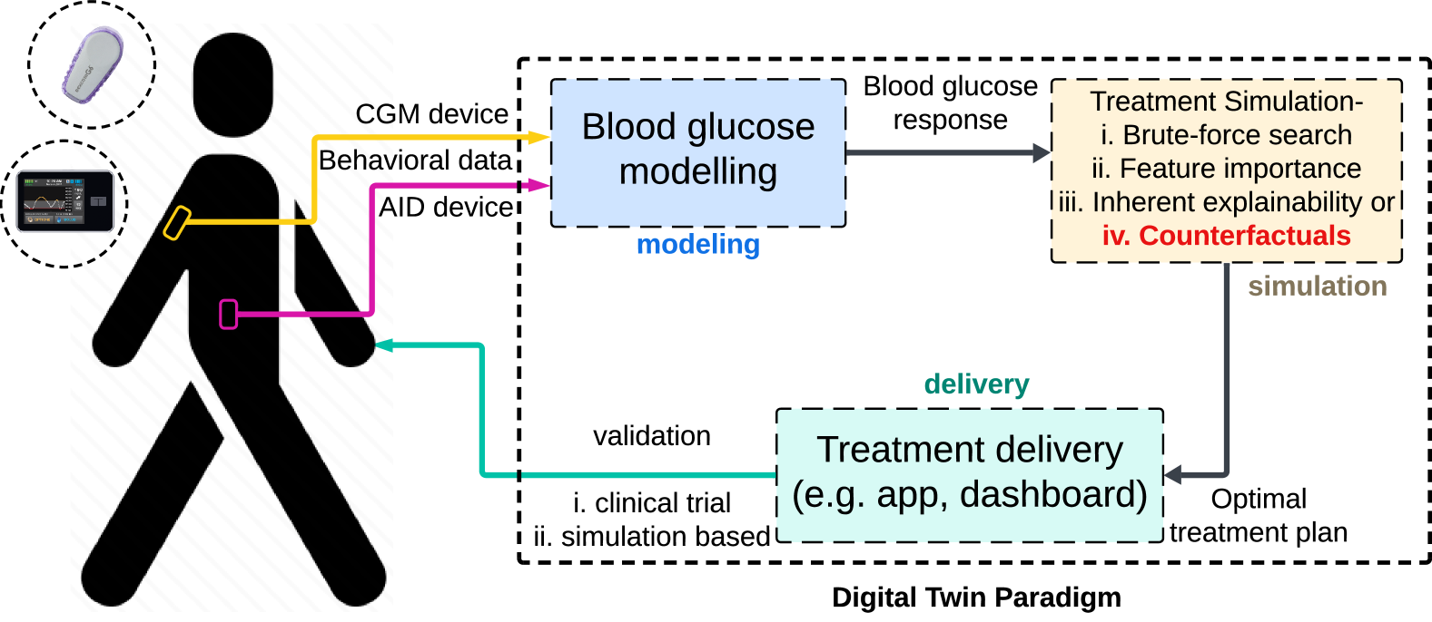
Figure 1: Digital twin framework with enhanced capabilities that can model physiological response, simulate treatments, and identify optimal treatment.

Our proposition, GlyTwin, is built upon this vision. Following Figure 1, we envision that a digital twin framework for glucose control in T1D comprises of three main pillars focused on modeling of blood glucose response, simulation of behavioral treatments, and delivery of optimal treatments. Prior research has primarily focused on blood glucose modeling by designing machine learning models that predict blood glucose levels based on past behavioral and physiological data [6, 7, 8, 11]. While a machine learning model can be potentially used to generate simulated interventions by modifying the inputs of the model and observing the glucose response at the model output, the number of candidate treatments under this approach is exponentially high. Specifically, for a machine learning model with $n$ inputs, there are $2^{n}$ permutations of the inputs that one can modify in order to generate an output for the model. Additionally, for each permutation of the inputs, there could be an exponential number of different values that each input permutation can take. As shown in Figure 1, one approach to identifying the optimal set of model inputs that can be chosen for behavioral intervention is to conduct a brute-force search on this highly exponential search space. However, this approach will be computationally infeasible for real-world deployment. Our approach for identifying optimal treatments relies on generating counterfactual explanations, a computationally-efficient machine learning approach to investigate how a desired outcome from a model can be obtained by generating new feature inputs.

We propose to extend the capabilities of the existing digital twin technologies, which focus specifically on predictive models [12], and integrate intervention planning by identifying optimal model inputs that achieve a pre-defined glucose outcome (e.g., identifying minimal behavioral modifications that lead to in-range postprandial blood glucose response) through the generation of counterfactual explanations. Therefore, as shown in Figure 1, the enhanced paradigm can model physiological outcomes, simulate possible treatment plans, and identify optimal behavioral treatment pathways. Simulating treatment plans can be accomplished through optimal outcome search, using models that are inherently explainable (like decision tree and logistic regression) or by employing explainable AI methods. Searching for optimal outcomes in high-dimensional data can be non-trivial, inherently explainable models may produce incomplete guidance or intervention [13], while feature importance based methods may lack the granularity desired in intervention design. For example, traditional explainable AI (XAI) is more interested in identifying an individual feature that is most important in explaining the prediction outcome. As a result, the ability of popular model-agnostic feature importance estimation technologies like LIME [14], TIME [15], SHAP [16] and other similar techniques [17, 18, 19, 20, 21] are limited to creating a hierarchy of the most relevant input features from the model’s perspective. Often, these explanations are provided in view of low-level features that are hardly understandable from a human perspective [22], which undermines the main objective of XAI. Feature relevance has proved to be important in building trust in a model [23]. However, when it comes to implementing treatment plan in digital health, designing interventions requires more precise and granular explainability.

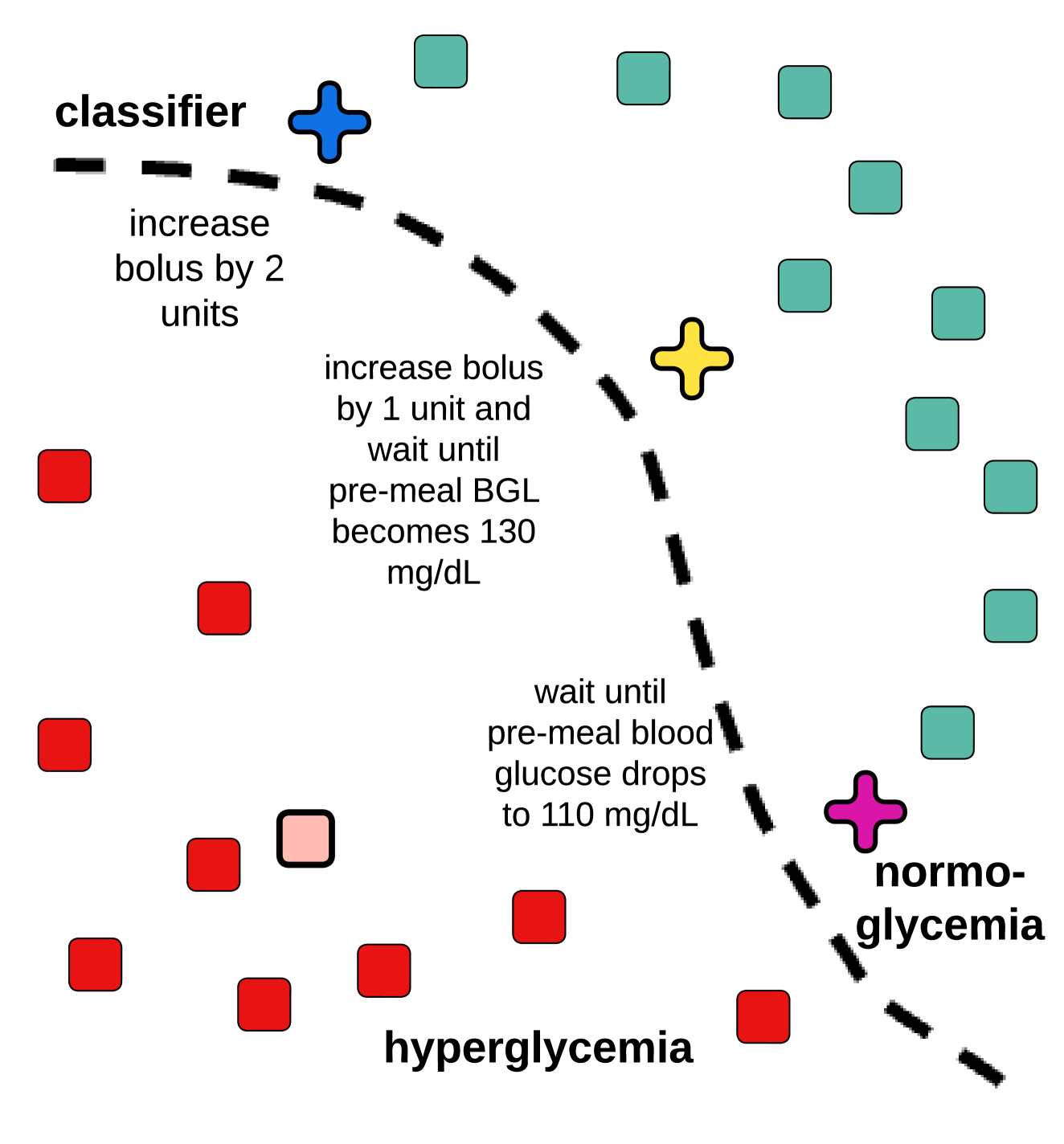
Figure 2: Counterfactual XAI for hyperglycemia prevention.

To provide granularity in interventions, counterfactual explanations (CFs) can serve as a feasible choice for treatment simulation. CF is a more targeted branch of XAI that emphasizes describing the smallest change to the feature values that alters the prediction to a desired output. CF instills trust in a model by explaining its way of decision making. Alternatively, the explanations themselves can be used to prevent adverse events from taking place. Figure 2 illustrates the core concept of CF based hyperglycemia prevention and how GlyTwin leverages counterfactual reasoning to generate actionable recommendations for patients and caregivers. Each square in the figure represents a glycemic outcome based on some behavioral and physiological conditions (e.g. pre-meal blood glucose levels (BGL) and insulin bolus dosing). Red squares represent samples that resulted in hyperglycemia, while green squares correspond to normoglycemic outcomes. The black dashed curve denotes the decision boundary of the classifier that separates hyperglycemia from normoglycemia. Assuming the pink square as an observed hyperglycemic event, GlyTwin identifies multiple potential counterfactual behavioral modifications (marked by colored plus signs) that could have transformed this hyperglycemic outcome into a normoglycemic one. These counterfactuals may include: (i) increasing the pre-meal insulin bolus by two units (blue cross), (ii) increasing the bolus by one unit combined with waiting until the pre-meal BGL decreases to 130 mg/dL (yellow cross), and (iii) waiting until the pre-meal BGL drops to 110 mg/dL without modifying the bolus (purple cross).

The blue dashed arrows demonstrate the behavioral adjustment pathways to transition from the observed hyperglycemic event to each of these counterfactual normoglycemic scenarios. Thus, GlyTwin can accommodate patient preferences and behavioral flexibility while offering multiple actionable pathways to avoid hyperglycemia. For instance, a CF intervention from GlyTwin might say: “You can prevent hyperglycemia by increasing your bolus intake by 2 units, or eating after your blood glucose level drops to 110 mg/dL”.

CFs can be either actual instances from the training data [24, 25], or can be an hypothetical synthetic sample made with a combination of feature values [26, 27, 28]. In fact, the utility of CF interventions in diabetes research is not entirely new. Lenatti et al. showed that CFs significantly improve fasting blood sugar, systolic blood pressure, triglycerides and HDL among people at risk for diabetes [29]. In a separate study, authors generated CF recommendations related to a healthy lifestyle for preventing diabetes onset [30]. Xiang et al. produced realistic CFs for diabetes prevention leveraging variational autoencoders [31]. Shah et al. [32] used CFs to generate alternate cases where metabolic syndrome is absent. However, none of these prior research focused on glucose control by integrating use preferences into the process of generating counterfactual explanations. As a result, the actionable information generated using CFs in prior research is often infeasible, unrealistic and contradictory to domain knowledge [33].

The proposed GlyTwin framework enhances the scope of digital twin in preventing adverse health outcomes and incorporates user preference in the intervention process process. We propose CFs as a novel addition to digital twin systems capable of flipping the prediction outcome and empowering the users (e.g., patients, clinicians). Within GlyTwin, we propose CFs as a way of modifying behavioral pathways for hyperglycemia prevention. While existing digital twin paradigm is primarily focused on projecting glycemic responses to assist with intervention planning, GlyTwin explores behavioral trajectories and creates intervention plans based on modified behavioral factors. Additionally, GlyTwin takes stakeholders’ preferences - like those of patients and physicians - by integrating feature weight inputs with the model’s derived preferences into the CF generation process. Thereby, GlyTwin empowers patients to express their personal preferences, like keeping certain aspects of behavior unchanged, directly reflected in the interventions designed for them. Contributions made through the design of GlyTwin can be shortlisted as follows.

• GlyTwin equips digital twin systems with counterfactual explanations, thus providing a means for treatment simulations. Using a novel model-agnostic and patient-centric algorithm, GlyTwin generates interventions aimed at preventing postprandial hyperglycemia through behavioral modifications (e.g., alternative behaviors in terms of eating time, carbohydrate amounts, insulin amount, and timing of insulin dosing).

• The interventions provided by GlyTwin are personalized, meaning that they reflect individuals’ preferences to withhold certain feature changes and operate within the individuals’ limitations in terms of behavioral preferences.

• GlyTwin is developed and tested extensively using a new clinical dataset collected in-the-wild and a competitive analysis is drawn against existing methods using standard validation metrics.

1 Results

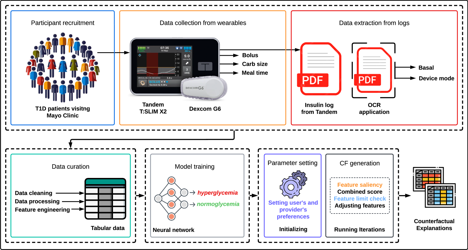
Figure 3: GlyTwin framework consists of four phases: data acquisition from CGM sensor and insulin logs, model training for glycemic outcome prediction, counterfactual generation for actionable recommendations, and integration into a dynamic, personalized management pipeline.

Table 1: Examples of processed samples from the dataset.

Age	Sex	Ethnicity	A1C	Carb size	Total bolus	$\Delta t$	Mode	Total basal	Pre-meal BGL slope	Pre-meal BGL	Outcome
61	F	White	6.7	20	7.57	-5	regular	2.475	2.943	129	normoglycemia
32	F	Hispanic	5	35	5.83	15	regular	0.357	1.457	134	hyperglycemia

We establish a pipeline to create the GlyTwin framework, which generates CF-based behavioral interventions for preventing hyperglycemia. A high-level overview of the pipeline is provided in Figure 3. Within the pipeline, we define distinct phases for data collection, data curation, model training, and CF generation.

The AZT1D dataset is constructed by obtaining data from patients with T1D at the Mayo Clinic Arizona who are on Automated Insulin Delivery (AID) systems. Information such as carbohydrate sizes, bolus doses, basal amounts, and device modes (e.g., sleep or exercise mode) is extracted from the obtained data. Next, we process the data to ensure quality and to derive additional variables. This step includes feature engineering, handling missing values, removing outliers, and formatting data for further analysis. Two processed samples are presented in Table 1. Of the eleven features, we consider Carb size, Total bolus, $\Delta t$, and Pre-meal BGL as modifiable factors for behavioral modification.

During the model development phase, a neural network is trained to classify outcomes as either hyperglycemia or normoglycemia based on input features. Although we choose a neural network for the classification task, GlyTwin is model-agnostic and can work with any model regardless of its architecture.

The CF generation phase begins with initializing GlyTwin. User and provider preference weights ($w_{u}$ and $w_{p}$) are set before we perform iterations to identify the desired CF intervention. During each iteration, GlyTwin identifies the feature that has the most impact on shifting towards normoglycemia when perturbed and applies perturbation ($\delta$) on it within the bounds. The iterations (and feature adjustments) continue until a confidence threshold ($\gamma$) towards normoglycemia is achieved. Therefore, the interventions generated by GlyTwin ensure minimal changes aligned with patient preferences and lead to the desired outcome.

1.1 Data Collection

A large pool of data has been collected from 100 patients with T1D who visited the Endocrinology Department of Mayo Clinic, Phoenix, AZ between December 2023 and April 2024 as part of their regular treatment (IRB #23-003065). For each patient, the data contains approximately $26$ days of recordings collected in free-living setting and includes CGM signals from Dexcom G6 Pro, insulin logs, meal carbohydrate sizes, and device modes (regular/sleep/exercise) from Tandem T:SLIM X2 Pump. Next, data from 21 randomly selected patients (Age: $57.4\pm 16.2$ years, $11$ female, A1C level: $5.0-8.2\%$, $18$ White and $3$ Hispanic) has been processed further for developing and testing GlyTwin. On average, each of these $21$ patients has $4.86$ hours of missing data segments which we avoided in the data analysis phase. Table 2 summarizes the demographics of patients in the AZT1D dataset.

Table 2: Demographic information of the AZT1D dataset collected from the Mayo Clinic.

n	Age (mean$\pm$SD)	Sex (F/M)	A1C (mean$\pm$SD)	YfD (mean$\pm$SD)	Ethnicity (White/Hispanic)
21	57.4$\pm$16.2	11/10	6.63$\pm$0.73	32.38$\pm$15.27	18/3

1.2 Classifier Performance

The dense net classifier trained on the data achieves an accuracy of $81\%$ and an F1-score of $80.4\%$. Using the F1-score metric is logical since the dataset is slightly imbalanced.

1.3 Quality of the counterfactuals

Table 3: Examples of some interventions made on hyperglycemic pre-meal contexts using GlyTwin.

Pre-meal context	Intervention
Tracey is a 41 year old white T1D patient with 6.3 A1C. She entered 18g carb size in her Tandem insulin pump and then got a bolus intake of 1.82 unit. Over the last 90 minutes, she took 1 unit basal. Somehow, she ate 45 minutes later when her pre-meal blood glucose reading was 70 mg/dL and blood glucose change rate was -3.18 mg/dL every 5 minute and pump was set at ’sleep’ mode. Eventually, she experienced post-meal hyperglycemia.	She could have prevented it just by taking the bolus 5 minutes before meal.
Rachel is 67 with an A1C of 6.6. Her last bolus shot was 4.1 units, taken before her meal which had 41 g carb size. She took 0.46 units of basal insulin over the last 90 minutes, and her pre-meal blood sugar level became 113 mg/dL. She experienced hyperglycemia after the meal.	With 7.69 units of bolus and 100 mg/dL pre-meal blood glucose level, Rachel could have prevented hyperglycemia.

Table 4: Evaluating the CFs on AZT1 Data: GlyTwin outperforms others in validity, NN test, proximity (except NICE as it identifies CFs from the training data), violations and achieves comparable results in sparsity and plausibility.

Method	Validation metrics
	validity $\uparrow$	NN test $\uparrow$	proximity $\downarrow$	sparsity $\downarrow$	violations $\downarrow$	plausibility $\uparrow$
GlyTwin	0.766	0.859	0.327	2.34	0	1.0
DiCE [34]	0.703	0.813	0.333	1.63	0	1.0
Optbinning [35]	0.61	0.578	0.333	3.06	0	0.91
CFNOW [36]	0.453	0.172	0.351	1.27	1.23	0.03
NICE [24]	0.688	0.688	0.179	1.875	0.41	0.9

Before proceeding with the validation of the generated CFs using established metrics, we first examine how GlyTwin’s CF interventions appear in a clinical setting. Table 3 presents sample interventions along with brief storytelling.

We next evaluate the CF interventions generated by GlyTwin by comparing them against similar works from the literature (e.g. DiCE [34], Optibinning [35], CFNOW [36], NICE [24]) using relevant metrics: (i) validity ($\uparrow$), which measures the proportion of the CFs that truly fall on the target class, (ii) NN test ($\uparrow$), which quantifies valid CFs leveraging historical outcomes of similar situations from patients, (iii) proximity ($\downarrow$) that measures distance from the factual sample, (iii) sparsity ($\downarrow$), which measures the complexity of the explanations, (iv) violations ($\downarrow$), which is a measure of non-modifiable feature changes and (v) plausibility ($\uparrow$) which indicates the proportion of the CFs that remain within the feature bounds. The summary in Table 4 outlines the quality of CFs generated by different methods. GlyTwin achieves an average validity that surpasses DiCE, NICE and CFNOW by $6.3\%$, $7.8\%$ and $31.3\%$, respectively. Note that, no technique gets a perfect score because the explanations are evaluated by the external simulator and not by the corresponding classifier. GlyTwin is ahead of the other techniques by at least $4.6\%$ as validated by historical data using NN test. Furthermore, the CFs produced by GlyTwin are at least $1.8\%$ closer to the test samples than those of DiCE, Optbinning and CFNOW. NICE does a better job in proximity because it identifies CFs from the real data which are actually closer to the factuals.

GlyTwin jointly leads the list for preserving the non-modifiable features with no feature violations per explanation. It ties with DiCE and achieves a perfect violations score. GlyTwin also leads the list for plausibility with a perfect score ($100\%$). This means that it can effectively keep the CFs within the original data manifold.

In terms of sparsity, our technique falls short as it changes more features per explanation compared to other methods. CFNOW achieves the best sparsity score because it mostly modifies A1C values which contributes to its poor plausibility and violations score. CFNOW does not allow keeping a subset of features unchanged.

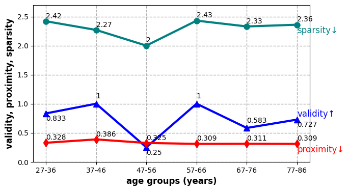
(a) Classification by patient age

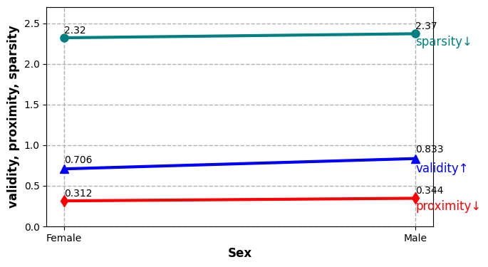
(b) Classification by patient sex

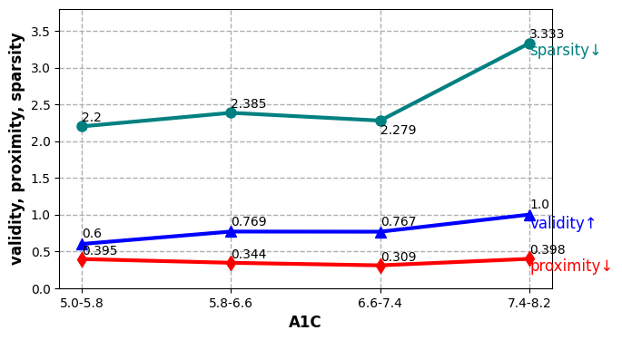
(c) Classification by patient A1C

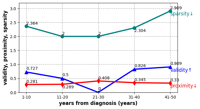
(d) Classification by years from diagnosis

Figure 4: Categorizing the performance of GlyTwin based on patient age, sex, A1C and years from diagnosis (YfD).

1.4 Classifying the results

Results from Table 4 are further classified by patient age, sex, A1C and years from diagnosis in Figures 4(a), 4(b), 4(c), 4(d), respectively. Notably, younger T1D patients ($27–46$ years) tend to experience smaller postprandial excursions, which helps GlyTwin to suggest effective interventions and score improved validity compared to that of the older populations. Specifically, the $37–46$ age group achieves perfect validity ($1.0$). However, the $47–56$ age group shows poor validity ($0.25$) likely due to the small sample size (only 4 patients, 3 of whom are false negatives). Proximity values remain relatively consistent across age groups, with younger patients ($27–36$ years) showing slightly higher proximity values ($0.328$). Sparsity, which reflects the simplicity of the CFs, does not vary significantly and stays within a narrow range of $2.0-2.43$ across all age groups.

When classified by sex (Figure 4(b)), validity scores indicate that GlyTwin performs better for males ($0.833$) than for females ($0.706$). Interestingly, females exhibit slightly better proximity scores ($0.312$) compared to males ($0.344$) meaning that CFs for females are more aligned with the original test data. Sparsity values remain similar for both sexes.

Results classified by patient A1C levels are shown in Table 4(d). Patients with lower A1C values ($5.0–5.8\%$) have lower validity ($0.6$) compared to those with higher A1C values ($7.4–8.2\%$), where validity reaches $1.0$. This suggests that patients with tighter glycemic control have less room for actionable CFs, while individuals with higher A1C exhibit more opportunities for improvement. Sparsity increases with A1C and peaks at $3.333$ for $7.4–8.2\%$ group.

In Figure 4(d), patients with 41–50 years since diagnosis achieve the highest validity ($0.909$), which indicates that GlyTwin performs better in individuals with long-term and stable glucose patterns. Proximity scores are slightly lower for those diagnosed within $1–20$ years but increase for patients who are into diabetes for $21–30$. Sparsity remains relatively high for patients who are $41-50$ years into diabetes.

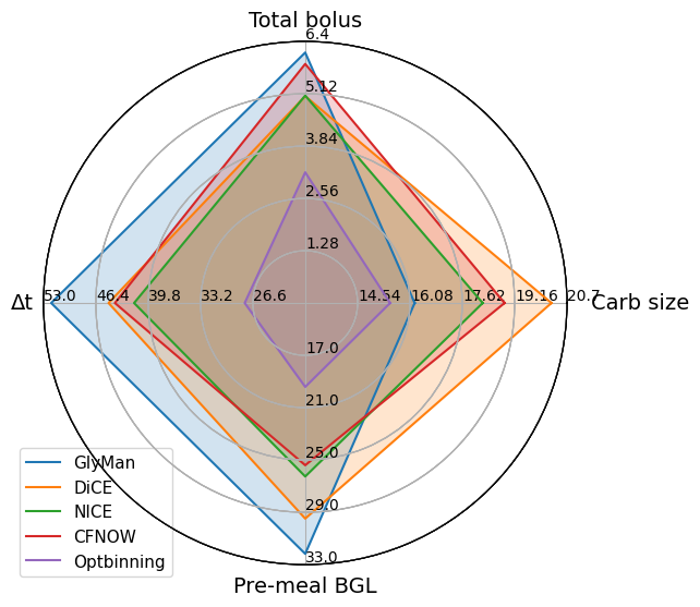
Figure 5: Comparison of feature diversity among CFs produced using different techniques.

1.5 Diversity of the counterfactuals

Next, we assess GlyTwin’s performance in terms of feature diversity. Although GlyTwin does not optimize for improving feature diversity, as shown in the radar plot of Figure 5, it exhibits better feature diversity for three out of the four modifiable features. Higher feature diversity means the CFs are exploring the entire the data and not limited to a specific subset of values for each feature.

1.6 Alignment with the preference weights

To understand if CFs from GlyTwin align with stakeholders’ preferences, we randomly set physician’s ($w_{p}$) and user’s preference weights ($w_{u}$) to [0, 0.9, 0.9, 0] and [0.1, 1, 1, 0.7], respectively, for carb size, total bolus, $\Delta t$ and pre-meal blood glucose level. We monitor the absolute changes in the corresponding features, normalize both the combined preference weights and the feature changes and plot them in Figure 6. The two variables are somewhat correlated, despite the impact of feature saliency.

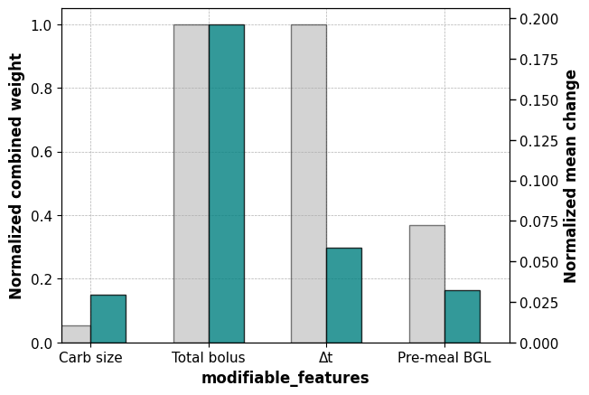
Figure 6: Preference alignment analysis of GlyTwin.

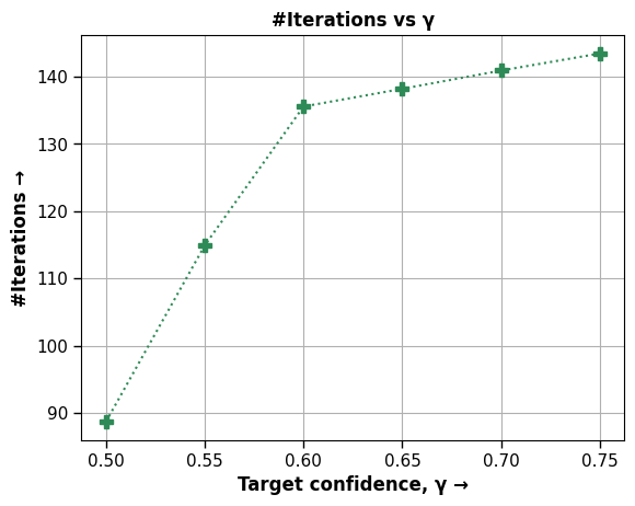
(a)

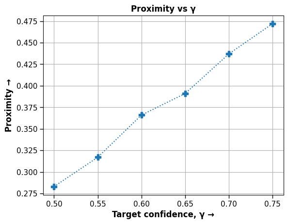
(b)

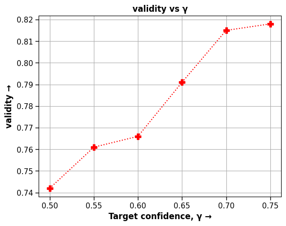
(c)

Figure 7: Results of ablations studies performed using GlyTwin. The ablation studies include understanding (a) how the number of required iterations, (b) proximity, and (c) validity changes as we set different target confidence for achieving normoglycemia.

2 Discussion

In this section, we will demonstrate some experiments conducted on the GlyTwin algorithm. Basically, we want to answer- what happens when certain parameters of GlyTwin are modified?

2.1 Impact of target probability

When a higher target probability ($\gamma$) is set for normoglycemia, it takes longer for GlyTwin to reach the target. Therefore, GlyTwin has to operate for additional iterations to converge. At the same time, converging to a higher target probability requires making more changes to the original factual sample which results in a higher proximity score. Furthermore, these additional iterations and proximity scores solidifies the CF’s position in the simulated validation with a higher validity score. Figure 7(a), 7(b), and 7(c) depict how number of iterations, proximity score and validity, respectively, change as we increase $\gamma$ from $0.50$ to $0.75$. For $\gamma=0.75$ validity of the generated CFs reaches as high as $0.82$ as determined by the external simulator.

2.2 Impact of perturbation size $\delta$

In this segment, we vary $\delta$ from $5\%$ to $25\%$ of the feature ranges and run GlyTwin algorithm to understand the impact of $\delta$ on the validation metrics. The summary of the impact is depicted in Table 5.

Validity peaks when $\delta\text{ is }10\%$ of the feature range. Other than that it remains close to $0.8$. With higher $\delta$, GlyTwin makes significant leaps from the factual point. Thus, there is a trade-off between validity and proximity. While higher $\delta$ improves validity, it simultaneously worsens proximity ranging from 0.152 at $\delta=5\%$ to $0.184\text{ at }\delta=25\%$ of feature range. Sparsity is somewhat robust to perturbation size as it remains stable across all $\delta$ values with narrowly increasing from $1.755$ to $1.776$. Quite understandably, runtime decreases significantly as $\delta$ increases, dropping from $14.224$ seconds at $\delta=5\%$ to $3.856$ seconds at $\delta=20\%$, before increasing slightly at $\delta=25\%$.

Therefore, $\delta$ needs to be large enough to make a difference and converge faster but not so large that it introduces incorrect changes or takes the CFs far from the factual samples.

Table 5: Scores for Different Delta Values

$\delta$ (%)	Validity	Proximity	Sparsity	Runtime (s)
5	0.796	0.152	1.776	14.224
10	0.857	0.161	1.755	8.085
15	0.816	0.171	1.755	7.380
20	0.776	0.181	1.755	3.856
25	0.833	0.184	1.771	9.379

2.3 How long does GlyTwin take?

Since some features are already at the terminal values or deemed non-modifiable, not all factual samples can converge to corresponding CF samples, regardless of the number of iterations. However, for samples where convergence is achievable, we can empirically show that on average GlyTwin generates actionable CFs in approximately $9.4$ seconds. Figure 8 compares runtime of samples that converge to CFs against the ones that do not.

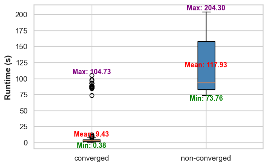
Figure 8: Runtime comparison between converged and non-converged samples. GlyTwin takes roughly $9.4$ seconds on average to produce a behavioral intervention to prevent hyperglycemia.

2.4 Limitations of GlyTwin

Although GlyTwin achieves promising results in many performance metrics, we have identified three limitations associated with the current state of the GlyTwin technology.

2.4.1 Clinical validation of the interventions

The main limitation of GlyTwin is that the generated CFs have not been clinically tested. The results obtained using a machine learning emulator mimics the intervention impact with reasonable confidence because the model is trained using data from the same distribution as the intervention data (i.e., future data obtained from the same patient). However, this analysis does not take into account patient’s adherence to the provided behavioral intervention. Therefore, the true impact of the interventions in preventing post-meal hyperglycemia also relies on the patients’ ability to follow them. Designing an AI-driven intervention is challenging, but transitioning it to real-world settings is even more challenging with issues like scalability, application development, regulatory compliance, user adaptability, and maintenance. Therefore, this study focuses solely on the development phase and simulation aided validations of GlyTwin.

2.4.2 Suggested $\Delta t$ values

Another limitation is that the CFs generated by GlyTwin often suggest delaying the bolus intakes i.e. taking the bolus after meals. While we do not have a concrete explanation for such interventions, our assumption is that delaying the bolus intake could help avoid insulin stacking. Insulin stacking occurs when multiple insulin doses are taken in close proximity and leads to increased risk of hypoglycemia. Insulin stacking is highly prevalent in our data and delayed bolus recommendations are highly correlated with factual instances where insulin stacking took place.

2.4.3 Higher computation cost

Since GlyTwin is an iterative algorithm, it has higher computation overhead. It is also a multi-step technique consisting of model training and adjusting the perturbations. Therefore, it is not fast compared to methods that train both the classifier and the generative model jointly and invokes the pipeline during inference [37].

3 Methods

Within the methods, we will formally define the problem we are trying to address as well as the solution we want to establish with GlyTwin .

3.1 Problem statement

Assume that $\mathcal{D}$ = {($X_{1}$,$y_{1}$), ($X_{2}$, $y_{2}$), $\dots$ , ($X_{n}$, $y_{n}$)} be a dataset of $n$ instances that has longitudinal health observations related to eating events and the corresponding health outcome such as blood glucose level categories. Each instance $X_{i}$ = [${x_{i}}^{1}$, ${x_{i}}^{2}$, $\dots$, ${x_{i}}^{d}$] consists of $d$ features including actionable behavioral parameters (e.g., diet, medication) and non-actionable parameters (e.g., age, gender, A1C). Considering $c$ possible classes for health outcome $Y$, where $y_{i}\in[1,c]$, a probabilistic AI model or classifier $f$ can be trained to map the $d$-dimensional input features to the $c$ classes and give us their corresponding prediction probabilities $f_{1},f_{2},\dots,f_{c}$:

$$f:\mathbb{R}^{d}\rightarrow[1,c]$$

Given a test sample $X_{T}$ predicted to indicate post-prandial hyperglycemia (i.g., ${\mbox{argmax}}f(X_{T})$ = $hyperglycemia$), a key question emerges: how to develop an effective intervention plan that empowers the patient to make informed behavioral changes to prevent the impending hyperglycemia while also preserving their preferences simultaneously?

3.2 Problem solution

To generate CFs, we have to go thorough several constrains and satisfy them. For example, the CFs must belong to the desired class, must not change too much from the factuals and must reflect user preferences. We assume that the stakeholder’s preferences for behavior changes are represented in vector $R(X_{T})$ = {$r_{1}$, $\dots$, $r_{d}$}, where each $r_{i}\in[0,1]$ represents the relative importance of the $i$-th feature for modification during intervention. Specifically, a value of $r_{i}=1$ indicates that the stakeholders strongly favor modifying the $i$-th feature, while $r_{i}=0$ implies no preference for modification. Our goal in GlyTwin is to generate CFs $(X_{T}^{*})$ that satisfy the following criteria:

• interventional: $X_{T}^{*}$ must change the class of the initial prediction from hyperglycemia to normoglycemia;

• minimal: $X_{T}^{*}$ must be minimally distant from the hyperglycemic factual sample $X_{T}$;

• partial: $X_{T}^{*}$ must favor stakeholders’ preferences expressed in feature weights $R$ and

• plausible: $X_{T}^{*}$ must be realistic, i.e., the features of the CFs must fall within the distribution of the dataset $\mathcal{D}$.

We formulate the CF generation process using a multi-objective optimization problem as shown in Equation (1), where the interventional, minimal, partial, and plausible requirements are formalized in the first to third terms, respectively.

$$\min_{X_{T}^{*}}\Big{[} CE\big{(}f_{n}(X_{T}^{*}),\overrightarrow{n}\big{)}+R\odot|X_{T}^{*}-X_{T}|+d\big{(}X_{T}^{*},X\big{)}\Big{]}$$ (1)

Here, $CE(\cdot)$ is the crossentropy loss between model’s prediction on the CF and normoglycemia, $d(\cdot)$ is the distance function.

For any test sample $X_{T}\in\mathbb{R}^{d}$ classified as hyperglycemia, the key idea would be finding the smallest adversarial perturbation $\delta_{min,p}$, that can be added to $X_{T}$, such that the perturbed point $X_{T}+\delta$ remains within a specified set of constraints $C$ and the classifier decision changes to $normoglycemia$. Therefore, the minimal adversarial perturbation for $X_{T}$ with respect to the $l_{p}$-norm can be defined mathematically-

$$\delta_{min,p} =\min_{\delta\in\mathbb{R}^{d}}||\delta||_{p}$$

s. t. $$f_{n}(X_{T}+\delta)>\max_{h\neq n,\forall a}f_{h}(X_{T}+\delta),\text{ }X_{T}+\delta\in C$$

To solve the optimization problem (1) using adversarial perturbation, we employ an iterative approach, where we adjust the features of $X_{T}$ step-by-step based on the saliency scores, stakeholder preferences, and the need to keep changes within realistic bounds.

One of the key objectives of CF generation is to make minimal changes to the factual samples. In that sense, feature saliency represents the impact of changing a specific feature on the model’s prediction for the target class. Therefore, identifying the most salient feature on each iteration helps GlyTwin determine which feature, when modified, will most significantly influence the prediction towards the desired outcome. This is achieved by calculating the forward derivative of the model’s prediction with respect to each feature.

For each modifiable feature in $x_{mod}$, the saliency score $S(x_{T},y^{\prime},i)$ is calculated by perturbing the feature value by a small amount and observing the change in the model’s prediction probability for the target class. This change is captured through the forward derivative of the prediction with respect to the feature,

$$S(x_{T},y^{\prime},i)=\frac{f_{n}(x_{T}^{*i}+\delta_{i})-f_{n}(x_{T}^{*i})}{\delta_{i}}\quad\forall x_{T}^{*i}\in x_{mod}$$ (2)

Leveraging the feature saliency, along with stakeholders’ preference weights, a combined score is calculated to determine the feature to be changed. Specifically, the combined score $C_{i}$ for each feature $x_{T}^{i}$ is computed by adding the normalized saliency score $S(x_{T}^{*},y^{\prime},i)^{\prime}$ (normalized to the range $\left[-1,1\right]$) to the sum of the physician’s and the user’s preference weights ($w_{p}$ and $w_{u}$), which later helps determine the feature to modify-

$$i^{\prime}=\arg\max_{i}\bigl{[}\left|S(x_{T}^{*},y^{\prime},i)^{\prime}\right|+(w_{p}+w_{u})\bigr{]}$$

$$x_{T}^{*i^{\prime}}=x_{T}^{*i^{\prime}}+\delta_{i}\text{ s. t. }\mathfrak{f}_{min}[i^{\prime}]\leq x_{T}^{*i^{\prime}}\leq\mathfrak{f}_{max}[i^{\prime}]$$

Algorithm 1 Generating Counterfactual explanationss with GlyTwin

1:Original observation $X_{T}=[x_{T}^{1},\dots,x_{T}^{d}]$, target class $y^{\prime}$, model $f$, maximum iterations $N$, target confidence for normoglycemia $\gamma$, perturbation/step sizes $\delta=[\delta_{1},\dots,\delta_{d}]$, indices of modifiable features $I_{mod}$, feature min values $\mathfrak{f}_{min}$, feature max values $\mathfrak{f}_{max}$, physician’s preference weights $w_{p}$, user’s preference weights $w_{u}$, multiplier $\mathcal{M}=[1,\dots,1]_{d}$

2:Counterfactual $X_{T}^{*}=[x_{T}^{*1},\dots,x_{T}^{*d}]$

3:$X_{T}^{*}\leftarrow X_{T}$

4:$n\leftarrow 0$ $\triangleright$ Track the number of iterations

5:while $f(X_{T}^{*})[y^{\prime}]<\gamma$ and $n<N$ do

6:  $S\leftarrow[0,\dots,0]_{d}$ $\triangleright$ Initialize saliency scores

7:  $C\leftarrow[0,\dots,0]_{d}$ $\triangleright$ Combined score for features

8:  for  $i\in I_{mod}$ do

9:   $X_{T}^{*^{\prime}}\leftarrow X_{T}*$

10:   $x_{T}^{*i^{\prime}}\leftarrow x_{T}^{*i^{\prime}}+\delta_{i}$

11:   $S_{i}\leftarrow\frac{f_{n}(X_{T}^{*^{\prime}})[y^{\prime}]-f_{n}(X_{T}^{*})[y^{\prime}]}{\delta_{i}}$ $\triangleright$ Feature saliency

12:   $C_{i}\leftarrow\left[|S_{i}|+w_{p}[i]+w_{u}[i]\right]\cdot\mathcal{M}[i]$

13:  end for

14:  $i\leftarrow\arg\max(C)$

15:  $x_{T}^{*i}\leftarrow x_{T}^{*i}+\text{sign}(S_{i})\cdot\delta_{i}$

16:  if $x_{T}^{*i}<\mathfrak{f}_{min}[i]$ then

17:   $x_{T}^{*i}\leftarrow\mathfrak{f}_{min}[i]$

18:   $\mathcal{M}[i]\leftarrow 0$

19:  else if $x_{T}^{*i}>\mathfrak{f}_{max}[i]$ then

20:   $x_{T}^{*i}\leftarrow\mathfrak{f}_{max}[i]$

21:   $\mathcal{M}[i]\leftarrow 0$

22:  end if

23:  $n\leftarrow n+1$

24:  if stopping criteria is met then

25:   break

26:  end if

27:end while

28:return $X_{T}^{*}$

$i^{\prime}$ denotes the index of the feature with the highest combined score. With this approach the feature selected for modification is both highly salient for the model and aligned with the stakeholders’ preferences. Next, we increment the selected feature with preset step size $\delta_{i}$. While doing so, we make sure the feature value is bounded below and above by predetermined limits, $\mathfrak{f}_{min}[i^{\prime}]$ and $\mathfrak{f}_{max}[i^{\prime}]$, respectively.

Finally, we add a stopping criteria to ensure that the algorithm terminates when it continues to make no improvements on the target class prediction for several rounds.

Algorithm 1 executes this iteration-based intervention search, ensuring that minimum and within-range changes are made only to features that maximize the combined score of feature saliency and stakeholder weights. Figure 3 explains the overall framework for GlyTwin.

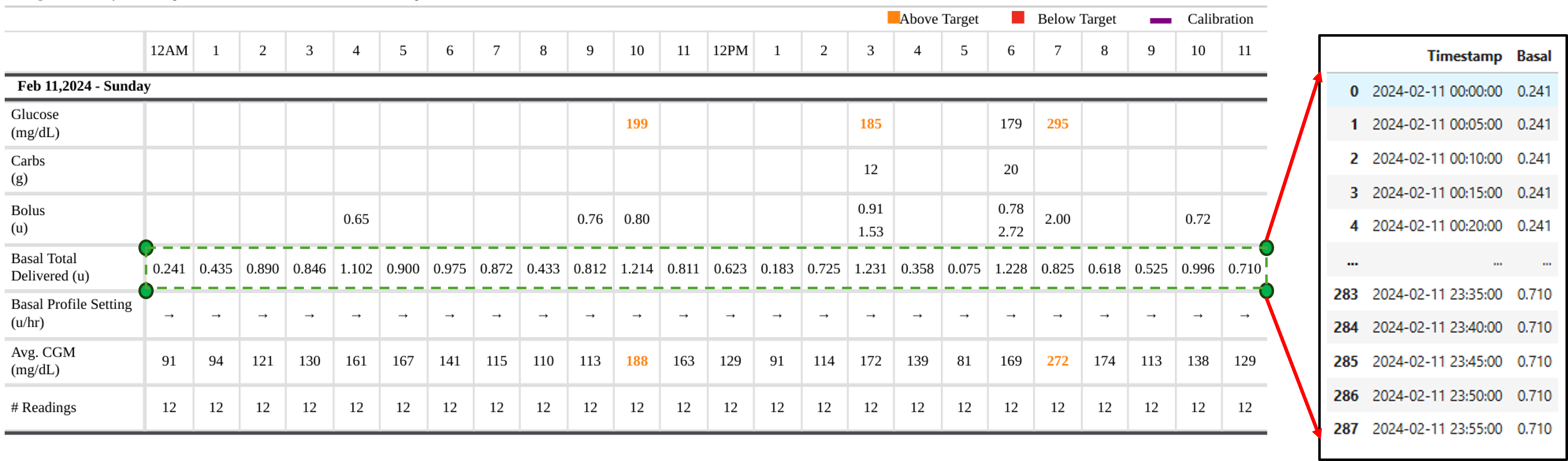
(a) Basal rate extraction

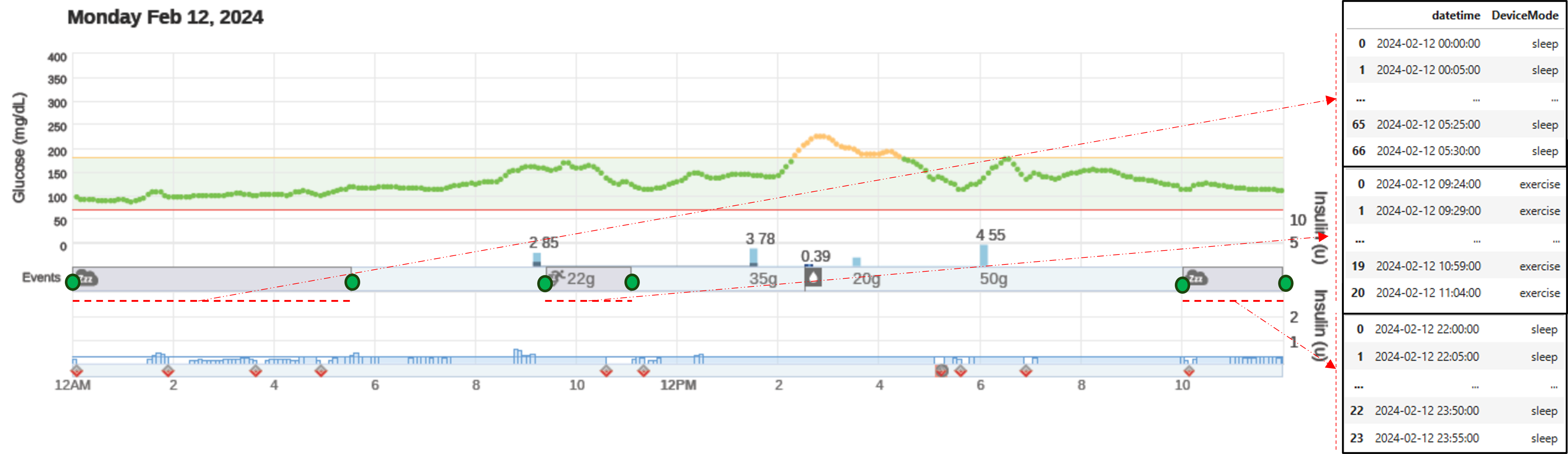
(b) AID device mode extraction

Figure 9: Extracting the basal rates and the device modes from the PDFs using OCR and coordinate system.

3.3 Data Processing

3.3.1 Basal rates and device modes

The hourly basal rates and device modes in the PDF files downloaded from Tandem are extracted by cropping the informative areas and then using an Optical Character Recognition (OCR) technique. Figures 9(a) and 9(b) shows the extraction process of basal rates and device modes using OCR and coordinate system.

3.3.2 Time between meal and food bolus, $\Delta t$

Prior research [38, 39, 40] says nearly $32\%$ T1D patients bolus after or during the meal which is one of the key reasons behind post-meal hyperglycemia. So, making suggestions on improving $\Delta t$ may play a key role in improving glycemic control.

To estimate $\Delta t$, first, the timestamps ($t_{fb}$) for food boluses have been identified from the timeseries data. Following two hours of $t_{fb}$, the maximum post-meal glycemic response and its timestamp ($t_{max}$) have been captured. Therefore, $BGL_{max}=\max(BGL[t_{fb}:t_{fb}+120])$ and $t_{max}=\arg\max(BGL[t_{fb}:t_{fb}+120])$. Since, peak time for glucose level after meal is $72\pm 23$ minutes, our assumption is that meal timestamp $t_{meal}=t_{max}-72$ [41]. Hence, we calculate $\Delta t$ using $t_{meal}$ and $t_{fb}$.

3.3.3 Total bolus

Total bolus is the sum of all bolus intakes taken between $\min(t_{meal},t_{fb})$ and $t_{max}$.

3.3.4 Total basal

Sum of all basal units taken between $t_{meal}-90$ and $t_{meal}$ falls under Total basal feature.

3.3.5 Pre-meal glucose level and slope

The CGM reading at $t_{meal}$ is the pre-meal blood glucose level. A linear trend-line is fitted using the prior 30 minutes’ ($t_{meal}-30:t_{meal}$) glucose readings and the pre-meal glucose level slope (or blood glucose change rate every 5 minute) is calculated from it.

3.3.6 Filtering out carb sizes

Oftentimes, patients intends to compensate for their high blood sugar levels with additional doses of food boluses instead of administering correction boluses. This scenario leads some secondary carb sizes in close vicinity of the primary one. On those occasions, we take the carb size with maximum value into account and neglect the rest that fall within $\min(t_{meal},t_{fb})$ and $t_{max}$.

All the above mentioned features and calculations are illustrated in Figure 10. The data processing pipeline leaves us with 1361 (722 hyperglycemic, 639 normoglycemic) factual samples, two of these samples are already shown in Table 1 as examples.

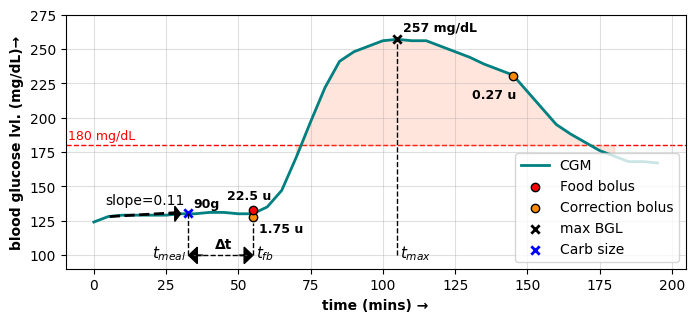
Figure 10: Derivation of different features from the data stream.

3.4 Classifier Details

The fully-connected binary classifier for hyperglycemia classification is described in Table 6.

Classifier hyperparameters are tuned on a trial-and-error basis. Results are generated after identifying the best set of hyperparameters. All experiments are done with an AMD Ryzen 7 2700X Eight-core CPU of 3.7 GHz speed, an NVIDIA GeForce GTX 1660 Ti GPU and 16 gigabyte RAM.

Table 6: Classifier specifications for hyperglycemia prediction.

Layer	Description
Input Layer	Dense, $64$ neurons, relu activation, HeNormal initializer, Batch normalization, Dropout rate: $0.4$
Hidden Layer 1	Dense, $32$ neurons, relu activation, HeNormal initializer, Batch normalization, Dropout rate: $0.4$
Hidden Layer 2	Dense, $32$ neurons, relu activation, HeNormal initializer, Batch normalization, Dropout rate: $0.4$
Output Layer	Dense, $2$ neurons, sigmoid activation
Optimizer	Adam, learning rate: $0.001$
Dataset Split	$85\%$ training set, $15\%$ test set
Training	$400$ epochs, batch size: $16$

3.5 Parameter set

Algorithm 1 contains multiple parameters that need to be initialized prior to running it. For preventing hyperglycemia, we set target class $y^{\prime}=$ normoglycemia and the corresponding confidence ($\gamma$) at $0.6$ as this value of $\gamma$ maintains a delicate balance between validity and proximity. We set the maximum iterations to $N=200$, and consider four features modifiable: Carb size, Total bolus, $\Delta t$, and Pre-meal BGL. Their corresponding perturbation size, $\delta$ values are $5$ grams, $0.5$ unit, $5$ minutes, and $10$ mg/dL, respectively. We personalize the minimum and maximum values for the modifiable features according to individual patients, but set the minimum and maximum pre-meal blood glucose levels to $100$ and $170$ mg/dL, respectively. When we compare GlyTwin against other techniques, unless mentioned otherwise, both the physician’s preference ($w_{p}$) and user’s preference weights ($w_{u}$) are set to $1$ for all modifiable features.

3.6 Baselines

We have identified the following techniques to compare against GlyTwin.

3.6.1 DiCE

DiCE [34] identifies a set of CFs by optimizing for proximity, diversity and sparsity.

3.6.2 Optbinning

In Optbinning [35], CFs are generated by optimizing binning rules to modify input features with an aim to find the shortest path to a target class.

3.6.3 CFNOW

CFNOW [36] searches an optimal point close to the factual point where the classification differs from the original. CFNOW performs greedy optimization for metrics like speed, coverage, distance, and sparsity.

3.6.4 NICE

CFs by NICE [24] are not necessarily adversarial data points but nearby instances in the data manifold that reflects the desired outcome.

3.7 Simulator specifications

The simulator used to estimate validity is an XGBoost model trained with real data. With a max-depth of $13$, learning rate of $0.1$, $100$ estimators and $85\%$ training data, the XGBoost simulator achieves $80.14\%$ accuracy.

4 Quantitative Measures

The quantitive analysis aims to rigorously evaluate the CFs generated by GlyTwin in terms of their alignment with desired outcomes, adherence to practical constraints, and interpretability. To ensure a comprehensive assessment, we employ a set of quantitative metrics widely used in the literature and adapt to the specific requirements of our application.

4.1 Validation Metrics

Validating the CFs has been a persistent challenge [42]. We assess the CFs using standard metrics found in the literature:

Validity assesses whether the produced CFs genuinely belong to the desired class [37]. High validity indicates the technique’s effectiveness in generating valid CF examples. Like [22], a simulation-aided method is designed to estimate the validity of the CFs.

$$\textit{validity}=\frac{\#|f(X_{T}^{*})\neq f(X_{T})|}{\|CF\|}$$

Nearest Neighbor Test (NN Test) validates the effectiveness of the CFs by comparing them against historical data to determine their likely outcomes (e.g., hyperglycemia or normoglycemia) based on past similar instances. We implement it using a k-nearest neighbor (k-NN) algorithm.

Proximity is the $L_{2}$ norm distance between $X_{T}$ and ${X_{T}}^{*}$. A low Proximity ensures we are making small change to the factual sample by preserving the details and not over-correcting the user [43].

$$\textit{proximity}=\sqrt{\sum_{i=1}^{m_{cont.}}\left(\frac{x_{T}^{*i}}{\|x_{T}^{*i}\|_{2}}-\frac{x_{T}^{i}}{\|x_{T}^{i}\|_{2}}\right)^{2}}$$ (3)

where: $m_{cont.}$ refers to the number of continuous features.

Sparsity is the average number of feature changes per CF. A low sparsity ensures better user understanding of the CFs [37].

$$\textit{sparsity}=\frac{\sum_{X_{T}^{*}\in CF}\sum_{i=1}^{d}\mathbbm{1}(x_{T}^{*i}\neq x_{T}^{i})}{\|CF\|}$$ (4)

Violations quantifies how frequently non-modifiable features (e.g. age, gender, insulin etc.) are changed. A good CF technique will have fewer violations per CF and promote fairness [44]. If $d_{\text{\textst{mod}}}$ is the number of non-modifiable features-

$$\textit{violations}=\frac{\sum_{X_{T}^{*}\in CF}\sum_{k=1}^{d_{\text{\textst{mod}}}}\mathbbm{1}(x_{T}^{*k}\neq x_{T}^{k})}{\|CF\|}$$ (5)

Plausibility estimates the fraction of explanations that fall within the feature ranges derived from the data [45]-

$$\textit{plausibility}=\frac{\sum_{X_{T}^{*}\in CF}\mathbbm{1}(\text{dist}(X_{T}^{*})\subseteq\text{dist}(X))}{\|CF\|}$$

where, dist($X_{T}^{*}$) and dist($X$) represent the distribution of feature values in the CF instances $X_{T}^{*}$ and in the training data, respectively. $\|CF\|$ is the total number of CF instances.

Finally, average feature diversity has been calculated using the following formula-

$$\text{Average diversity for feature }k=\frac{\sum_{i}\sum_{j}|{x_{i}}^{k}-{x_{j}}^{k}|}{\|CF\|},i\neq j$$

5 Conclusion

We proposed GlyTwin that refines the traditional digital twin technology with CFs and empowers stakeholders to participate in the CF generation process. GlyTwin is built and tested on real data collected in uncontrolled settings. Our analysis demonstrates that the generated CFs are valid, fair, realistic, and minimal, eventually matching or outperforming existing techniques in producing quality CFs. Our next venture includes overcoming the aforementioned limitations and have it trialed with real patients in a clinical setting.

6 Data Availability

Data gathered in this investigation are subject to data use agreements with parties involved in the study and are therefore not freely available.

7 Code Availability

Code has been made available in the following github repository: github.com/Arefeen06088/GlyTwin

References

- [1] Evan L. Reynolds, Kara R. Mizokami-Stout, Nathaniel Putnam, Mousumi Banerjee, Dana Albright, Lynn Ang, Joyce Lee, Rodica Pop-Busui, Eva L. Feldman, and Brian Christopher Callaghan. Cost and utilization of healthcare services for persons with diabetes. Diabetes research and clinical practice, page 110983, 2023.
- [2] Nuha A. ElSayed, Grazia Aleppo, Vanita R. Aroda, Raveendhara R. Bannuru, Florence M. Brown, Dennis Bruemmer, Billy S. Collins, Marisa E. Hilliard, Diana M. Isaacs, Eric L. Johnson, Scott Kahan, Kamlesh K Khunti, Jose Leon, Sarah K. Lyons, Mary Lou Perry, Priya Prahalad, Richard E. Pratley, J. Seley, Robert C. Stanton, and Robert A. Gabbay. 6. Glycemic Targets: Standards of Care in Diabetes-2023. Diabetes care, 46 Supplement_1:S97–S110, 2022.
- [3] Jennifer L. Sherr, Lori M. Laffel, Jingwen Liu, Wendy A. Wolf, Jeoffrey A. Bispham, Katherine S Chapman, Daniel Finan, Lina Titievsky, Tina Liu, Kaitlin Hagan, Jason L. Gaglia, Keval Chandarana, Richard M. Bergenstal, and Jeremy H. Pettus. Severe hypoglycemia and impaired awareness of hypoglycemia persist in people with type 1 diabetes despite use of diabetes technology: Results from a cross-sectional survey. Diabetes Care, 47:941 – 947, 2024.
- [4] Paramesh Shamanna, Ravi Sankar Erukulapati, Ashutosh Shukla, Lisa Shah, Bree Willis, Mohamed Thajudeen, Rajiv Kovil, Rahul Baxi, Mohsin Wali, Suresh Damodharan, and Shashank R Joshi. One-year outcomes of a digital twin intervention for type 2 diabetes: a retrospective real-world study. Scientific Reports, 14, 2024.
- [5] Zhouyu Guan, Huating Li, Ruhan Liu, Chun Cai, Yuexing Liu, Jiajia Li, Xiangning Wang, Shan Huang, Liang Wu, Dan Liu, Shujie Yu, Zheyuan Wang, Jia Shu, Xuhong Hou, Xiaokang Yang, Weiping Jia, and Bin Sheng. Artificial intelligence in diabetes management: Advancements, opportunities, and challenges. Cell Reports Medicine, 4, 2023.
- [6] Giacomo Cappon, Martina Vettoretti, Giovanni Sparacino, Simone Del Favero, and Andrea Facchinetti. Replaybg: A digital twin-based methodology to identify a personalized model from type 1 diabetes data and simulate glucose concentrations to assess alternative therapies. IEEE Transactions on Biomedical Engineering, 70:3227–3238, 2023.
- [7] Giacomo Cappon, Elisa Pellizzari, Luca Cossu, Giovanni Sparacino, Annalisa Deodati, Riccardo Schiaffini, Stefano Cianfarani, and Andrea Facchinetti. System architecture of twin: A new digital twin-based clinical decision support system for type 1 diabetes management in children. 2023 IEEE 19th International Conference on Body Sensor Networks (BSN), pages 1–4, 2023.
- [8] Naveenah Udaya Surian, Arsen Batagov, Andrew Wu, W. B. Lai, Yan Sun, Yong Mong Bee, and Rinkoo Dalan. A digital twin model incorporating generalized metabolic fluxes to identify and predict chronic kidney disease in type 2 diabetes mellitus. NPJ Digital Medicine, 7, 2024.
- [9] Oscar Silfvergren, Christian Simonsson, Mattias Ekstedt, Peter Lundberg, Peter Gennemark, and Gunnar Cedersund. Digital twin predicting diet response before and after long-term fasting. PLoS Computational Biology, 18, 2021.
- [10] Ziyi Zhou, Ming Cheng, Xingjian Diao, Yanjun Cui, and Xiangling Li. Glumarker: A novel predictive modeling of glycemic control through digital biomarkers. 2024 46th Annual International Conference of the IEEE Engineering in Medicine and Biology Society (EMBC), pages 1–7, 2024.
- [11] Asiful Arefeen and Hassan Ghasemzadeh. Glysim: Modeling and simulating glycemic response for behavioral lifestyle interventions. 2023 IEEE EMBS International Conference on Biomedical and Health Informatics (BHI), pages 1–5, 2023.
- [12] Syed Hasib Akhter Faruqui, Adel Alaeddini, Yan Du, Shiyu Li, Kumar Sharma, and Jing Wang. Nurse-in-the-loop artificial intelligence for precision management of type 2 diabetes in a clinical trial utilizing transfer-learned predictive digital twin. ArXiv, abs/2401.02661, 2024.
- [13] Asiful Arefeen, Samantha N Fessler, Carol Johnston, and Hassan Ghasemzadeh. Forewarning postprandial hyperglycemia with interpretations using machine learning. 2022 IEEE-EMBS International Conference on Wearable and Implantable Body Sensor Networks (BSN), pages 1–4, 2022.
- [14] Marco Tulio Ribeiro, Sameer Singh, and Carlos Guestrin. “why should i trust you?”: Explaining the predictions of any classifier. Proceedings of the 22nd ACM SIGKDD International Conference on Knowledge Discovery and Data Mining, 2016.
- [15] Akshay Sood and Mark W. Craven. Feature importance explanations for temporal black-box models. ArXiv, abs/2102.11934, 2021.
- [16] Scott M. Lundberg and Su-In Lee. A unified approach to interpreting model predictions. ArXiv, abs/1705.07874, 2017.
- [17] Zhengze Zhou and Giles Hooker. Unbiased measurement of feature importance in tree-based methods. ACM Transactions on Knowledge Discovery from Data (TKDD), 15:1 – 21, 2019.
- [18] Aaron Fisher, Cynthia Rudin, and Francesca Dominici. All models are wrong, but many are useful: Learning a variable’s importance by studying an entire class of prediction models simultaneously. Journal of machine learning research : JMLR, 20, 2018.
- [19] João Bento, Pedro Saleiro, Andre Ferreira Cruz, Mário A. T. Figueiredo, and P. Bizarro. Timeshap: Explaining recurrent models through sequence perturbations. Proceedings of the 27th ACM SIGKDD Conference on Knowledge Discovery & Data Mining, 2020.
- [20] Sana Tonekaboni, Shalmali Joshi, Kieran Campbell, David Kristjanson Duvenaud, and Anna Goldenberg. What went wrong and when? instance-wise feature importance for time-series black-box models. In Neural Information Processing Systems, 2020.
- [21] Saranya A. and Subhashini R. A systematic review of explainable artificial intelligence models and applications: Recent developments and future trends. Decision Analytics Journal, 2023.
- [22] Pietro Barbiero, Gabriele Ciravegna, Francesco Giannini, Pietro Li’o, Marco Gori, and Stefano Melacci. Entropy-based logic explanations of neural networks. ArXiv, abs/2106.06804, 2021.
- [23] Rich Caruana, Yin Lou, Johannes Gehrke, Paul Koch, M. Sturm, and Noémie Elhadad. Intelligible models for healthcare: Predicting pneumonia risk and hospital 30-day readmission. Proceedings of the 21th ACM SIGKDD International Conference on Knowledge Discovery and Data Mining, 2015.
- [24] Dieter Brughmans and David Martens. Nice: an algorithm for nearest instance counterfactual explanations. Data Mining and Knowledge Discovery, pages 1–39, 2021.
- [25] Abdullah Mamun, Lawrence D. Devoe, Mark I. Evans, David W. Britt, Judith Klein-Seetharaman, and Hassan Ghasemzadeh. Use of what-if scenarios to help explain artificial intelligence models for neonatal health. ArXiv, abs/2410.09635, 2024.
- [26] Lisa Schut, Oscar Key, Rory McGrath, Luca Costabello, Bogdan Sacaleanu, Medb Corcoran, and Yarin Gal. Generating interpretable counterfactual explanations by implicit minimisation of epistemic and aleatoric uncertainties. In International Conference on Artificial Intelligence and Statistics, 2021.
- [27] Asiful Arefeen and Hassan Ghasemzadeh. Designing user-centric behavioral interventions to prevent dysglycemia with novel counterfactual explanations. ArXiv, abs/2310.01684, 2023.
- [28] Asiful Arefeen, Saman Khamesian, María Adela Grando, Bithika Thompson, and Hassan Ghasemzadeh. Glyman: Glycemic management using patient-centric counterfactuals. 2024 IEEE EMBS International Conference on Biomedical and Health Informatics (BHI), pages 1–5, 2024.
- [29] Marta Lenatti, Alberto Carlevaro, Aziz Guergachi, Karim Keshavjee, Maurizio Mongelli, and Alessia Paglialonga. A novel method to derive personalized minimum viable recommendations for type 2 diabetes prevention based on counterfactual explanations. PLOS ONE, 17, 2022.
- [30] Marta Lenatti, Alberto Carlevaro, Karim Keshavjee, Aziz Guergachi, Alessia Paglialonga, and Maurizio Mongelli. Characterization of type 2 diabetes using counterfactuals and explainable ai. Studies in health technology and informatics, 294:98–103, 2022.
- [31] Xintao Xiang and Artem Lenskiy. Realistic counterfactual explanations by learned relations. ArXiv, abs/2202.07356, 2022.
- [32] Sanyam Paresh Shah, Abdullah Mamun, Shovito Barua Soumma, and Hassan Ghasemzadeh. Enhancing metabolic syndrome prediction with hybrid data balancing and counterfactuals. volume abs/2504.06987, 2025.
- [33] Aditya Bhattacharya, Jeroen Ooge, Gregor Stiglic, and Katrien Verbert. Directive explanations for monitoring the risk of diabetes onset: Introducing directive data-centric explanations and combinations to support what-if explorations. Proceedings of the 28th International Conference on Intelligent User Interfaces, 2023.
- [34] Ramaravind K Mothilal, Amit Sharma, and Chenhao Tan. Explaining machine learning classifiers through diverse counterfactual explanations. In Proceedings of the 2020 Conference on Fairness, Accountability, and Transparency, pages 607–617, 2020.
- [35] Guillermo Navas-Palencia. Optimal Counterfactual Explanations for Scorecard modelling. ArXiv, abs/2104.08619, 2021.
- [36] Raphael Mazzine Barbosa de Oliveira, Kenneth Sörensen, and David Martens. A model-agnostic and data-independent tabu search algorithm to generate counterfactuals for tabular, image, and text data. European Journal of Operational Research, 2023.
- [37] Hangzhi Guo, Thanh Hong Nguyen, and Amulya Yadav. CounterNet: End-to-End Training of Prediction Aware Counterfactual Explanations. Proceedings of the 29th ACM SIGKDD Conference on Knowledge Discovery and Data Mining, 2021.
- [38] Fraser Cameron, Günter Niemeyer, and Bruce A. Buckingham. Probabilistic evolving meal detection and estimation of meal total glucose appearance. Journal of Diabetes Science and Technology, 3:1022 – 1030, 2009.
- [39] John P. Corbett, Marc D. Breton, and Stephen D. Patek. A multiple hypothesis approach to estimating meal times in individuals with type 1 diabetes. Journal of Diabetes Science and Technology, 15:141 – 146, 2019.
- [40] Anne L. Peters, Michelle A Van Name, Brian Larsen Thorsted, Johanne Spanggaard Piltoft, and William V Tamborlane. Postprandial dosing of bolus insulin in patients with type 1 diabetes: A cross-sectional study using data from the t1d exchange registry. Endocrine practice : official journal of the American College of Endocrinology and the American Association of Clinical Endocrinologists, 23 10:1201–1209, 2017.
- [41] S. Daenen, Agnès Sola-Gazagnes, Jocelyne M’bemba, C Dorange-Breillard, F Defer, Fabienne Elgrably, Etienne Larger, and Gérard Slama. Peak-time determination of post-meal glucose excursions in insulin-treated diabetic patients. Diabetes & metabolism, 36 2:165–9, 2010.
- [42] Tim Miller. Explanation in Artificial Intelligence: Insights from the Social Sciences. Artif. Intell., 267:1–38, 2017.
- [43] Sandra Wachter, Brent Daniel Mittelstadt, and Chris Russell. Counterfactual Explanations Without Opening the Black Box: Automated Decisions and the GDPR. Cybersecurity, 2017.
- [44] Shuyi Chen and Shixiang Zhu. Counterfactual Fairness through Transforming Data Orthogonal to Bias. ArXiv, abs/2403.17852, 2024.
- [45] Riccardo Guidotti. Counterfactual explanations and how to find them: literature review and benchmarking. Data Mining and Knowledge Discovery, pages 1–55, 2022.