Score Matching Diffusion Based Feedback Control and Planning of Nonlinear Systems

Abstract

We propose a novel control-theoretic framework that leverages principles from generative modeling—specifically, Denoising Diffusion Probabilistic Models (DDPMs)—to stabilize control-affine systems with nonholonomic constraints. Unlike traditional stochastic approaches, which rely on noise-driven dynamics in both forward and reverse processes, our method crucially eliminates the need for noise in the reverse phase, making it particularly relevant for control applications. We introduce two formulations: one where noise perturbs all state dimensions during the forward phase while the control system enforces time reversal deterministically, and another where noise is restricted to the control channels, embedding system constraints directly into the forward process.

For controllable nonlinear drift-free systems, we prove that deterministic feedback laws can exactly reverse the forward process, ensuring that the system’s probability density evolves correctly without requiring artificial diffusion in the reverse phase. Furthermore, for linear time-invariant systems, we establish a time-reversal result under the second formulation. By eliminating noise in the backward process, our approach provides a more practical alternative to machine learning-based denoising methods, which are unsuitable for control applications due to the presence of stochasticity. We validate our results through numerical simulations on benchmark systems, including a unicycle model in a domain with obstacles, a driftless five-dimensional system, and a four-dimensional linear system, demonstrating the potential for applying diffusion-inspired techniques in linear, nonlinear and settings with state space constraints.

I Introduction

Feedback control of nonlinear systems remains a central challenge in control theory. Unlike linear systems, where stabilization techniques such as LQR, pole placement, and Lyapunov-based methods provide systematic solutions, nonlinear systems lack a unified stabilization framework due to inherent mathematical difficulties. These challenges arise from the need to construct Lyapunov functions [1], the non-convexity of optimal control formulations [2], and obstructions to stabilization using smooth, time-invariant feedback laws [3]. Although methods such as feedback linearization [4], Lyapunov-based control [5], and model predictive control [6] offer solutions in specific cases, they rely heavily on system structure and often fail in more general settings. The absence of a broadly applicable stabilization framework for nonlinear systems remains an open problem, motivating the search for alternative formulations of control problems.

Recent advances in machine learning, particularly in generative modeling, provide an alternative approach to control synthesis. Instead of directly solving high-dimensional optimization problems associated with nonlinear optimal control, generative models learn to synthesize system trajectories to match a desired probability distribution. Several techniques, including normalizing flows [7], Langevin-based sampling [8], and Markov chain Monte Carlo (MCMC) methods [9], have been explored for this purpose. However, these methods frequently suffer from numerical intractability when applied to high-dimensional, non-Gaussian distributions. The connection between generative modeling and control arises from the observation that sampling from a probability distribution can be viewed as a control problem in the space of probability densities. This connection suggests that techniques from generative modeling may provide useful insights for control synthesis.

Denoising Diffusion Probabilistic Models (DDPMs) [10, 11] have recently emerged as a powerful tool for generative modeling and offer an alternative approach to control. These models operate through a bidirectional diffusion process, where a forward phase progressively injects noise into the system, transforming the original distribution into an easily sampled Gaussian, and a reverse phase reconstructs the target distribution by inverting this transformation. The advantage of this framework is that it eliminates the need to solve an explicit optimal control problem, replacing it with a regression-based formulation that learns the reverse process directly. Given their success in high-dimensional generative modeling, DDPMs provide a natural foundation for rethinking nonlinear control, particularly for stabilization and trajectory planning.

This paper extends diffusion-based modeling techniques to control synthesis by reformulating finite-horizon control as a trajectory generation problem. Unlike conventional probability density control [12], which often requires solving computationally expensive optimal transport problems, the proposed approach leverages diffusion models to approximate the density evolution of the system. This allows for an efficient and scalable alternative to nonlinear optimal control, particularly in constrained and underactuated systems. By embedding control constraints into the reverse diffusion process, we provide a method for synthesizing trajectories that bypass the computational challenges of solving Hamilton-Jacobi-Bellman equations or nonlinear model predictive control formulations.

Diffusion-based methods have been widely explored in generative modeling, reinforcement learning, and trajectory planning. Recent work has demonstrated the use of DDPMs for generating trajectories by constructing probability densities over trajectory spaces. A key example is the approach by [13], which captures system dynamics over state-space sequences using diffusion-based methods. However, representing full trajectory distributions introduces scalability issues due to the high dimensionality of the space of state trajectories. In [14] address this challenge by directly learning sequences of action policies, thereby reducing the complexity associated with modeling full trajectory densities. Other refinements by [15] and [16] focus on structured planning problems, incorporating diffusion models tailored to robotic applications. In [17], we presented a method of incorporating the underlying dynamics for trajectory generation into diffusion-based planning. While these approaches leverage diffusion for long-horizon planning, they rely on applying noise to entire trajectory spaces, instead of the state. This leads to higher dimensionality when applied to control synthesis, since the set of trajectories lives in a higher dimensional space in comparison to the set of states.

In contrast, the approach proposed in this paper constrains the diffusion process to the state space while using the control system itself as the denoising mechanism. Instead of introducing noise into entire trajectory sequences, the method exploits the system’s structure to guide the reverse process. This formulation significantly reduces dimensionality, improving computational efficiency and control fidelity. Unlike existing diffusion-based trajectory planning approaches, which operate in purely data-driven settings, the proposed method incorporates system dynamics into the diffusion process, allowing for a more structured and interpretable control synthesis method.

The control of probability densities is an established problem in optimal transport and stochastic control, particularly in applications where system behavior is expressed in terms of distributions rather than individual trajectories. Several works have extended optimal transport techniques to control systems, such as those first initated by [18, 19] for nonlinear control systems. See also some later generalizations under weaker requirements on the control system and the cost functions by the first author [20, 21] or extensions of optimal transport for feedback linearizable systems [22]. These formulations seek to steer a probability distribution toward a desired target, but high-dimensional formulations frequently suffer from computational intractability. Related work by [23], [24] investigates probability density control for linear systems, where Gaussian distributions serve as natural attractors under certain constraints. However, these methods do not generalize well to nonlinear systems or cases where the target distribution is non-Gaussian. Other approaches use long-term behavior of closed-form mean-field feedback stabilization laws, such as those by [25], [26], while mean-field game theory and mean-field control extend these ideas to develop optimal control methods for large scale systems by using continuum limits, as seen in [27] and [28].

Despite these contributions, probability density control methods often rely on solving high-dimensional optimization problems, making them impractical for real-time control. Many existing formulations impose convexity constraints on the target distributions, which, when violated, lead to arbitrarily slow convergence rates. The approach presented in this paper circumvents these limitations by replacing optimization with a regression-based formulation. Rather than solving constrained optimization problems, the method leverages diffusion models to construct a deterministic reverse process that mimics the evolution of the desired probability density. Unlike classical probability density control, which often relies on stochastic perturbations, the proposed method embeds control constraints directly into the denoising process, enabling trajectory synthesis through deterministic system evolution. This makes it particularly suitable for stabilization tasks in nonlinear and underactuated systems.

By bridging the gap between generative modeling and control synthesis, this work provides a scalable alternative to classical nonlinear control methods. The proposed approach eliminates the need for solving Hamilton-Jacobi-Bellman equations or explicitly computing optimal control laws, instead using a data-driven approximation to construct stabilizing trajectories. Compared to existing generative modeling techniques, the method directly incorporates system dynamics, avoiding the scalability issues that arise in high-dimensional trajectory planning. This formulation represents a novel direction for applying diffusion-based techniques to nonlinear control, offering a computationally efficient and theoretically grounded framework for probability density evolution in constrained dynamical systems.

I-A Contribution

In this paper, we investigate the application of recent advances in generative modeling to control synthesis. Our main contributions are as follows:

1. DDPM-Based Control Formulation: We introduce a novel framework that reformulates the control problem using Denoising Diffusion Probabilistic Models (DDPMs), leveraging their bidirectional sampling process for trajectory generation and stabilization.

2. Conditions for a Deterministic Reverse Process: We establish conditions under which a feedback control law can enforce a valid deterministic reverse process, ensuring that the control system can precisely recover target distributions without stochastic perturbations.

3. Drift-Free Systems in Constrained Domains: For drift-free systems, we analyze control strategies constrained to compact sets, enabling simultaneous trajectory planning and global attractivity of target set in potentially non-convex state spaces.

   Our contributions include two Algorithms for denoising based control, which are presented in the next section. A partial analysis of Algorithm 1 has been presented in a conference version of this paper [29]. Particularly, Proposition IV.6, Lemma IV.7 and Lemma IV.8 appeared in the conference version.

II Problem setting and preliminary notions

Consider the control affine, nonlinear control system

$$\dot{x}=g(x,u)=g_{0}(x)+\sum_{i=1}^{m}g_{i}(x)u_{i},$$ (1)

where $x\in\mathbb{R}^{d}$ denotes the state of the system, $u_{i}$ the $i$-th control input, and $g_{i}\in C^{\infty}(\mathbb{R}^{d};\mathbb{R}^{d})$ are smooth vector fields. The model (1) is commonly used in robotics to describe the dynamics of ground vehicles, underwater robots, manipulators, and other non-holonomic systems [30]. In this paper we aim to solve a finite-time density control problem, that is, to find a control policy $u=\pi(t,x)$ such that the density of the state $x(T)$ is $p_{\text{target}}$ when the density of the initial state is $p_{n}$, for a given control horizon $T\in\mathbb{R}_{>0}$. To this aim, we propose a methodology that relies on recent DDPMs, where the control policy is given by a neural network whose output is a control policy that allows the system (1) to track the trajectories generated by reference stochastic diffusion process that ensures $x(T)\sim p_{\text{target}}$. To further clarify our approach, we next review denoising diffusion models through the lens of stochastic differential equations as presented in [11], and formally state the control problem of interest and its applications.

II-A Denoising Diffusion Probabilistic model

Denoising Diffusion Probabilistic Model (DDPM) is a generative modeling technique that learns to sample from an unknown data density $p_{\text{target}}$ by (i) transforming it into a known density $p_{n}$ from which one can easily sample (such density has been referred to as the noise density), (ii) sampling from it, and finally (iii) reversing the transformation. This is done using two stochastic differential equations. First, the forward process is a stochastic differential equation of the form

$$\textup{d}X^{\text{f}}=V(X^{\text{f}})+\sqrt{2}\,\textup{d}W+\textup{d}Z,$$ (2)

where $X_{0}$ has density $p_{\text{target}}$. In (2), $W$ denotes the standard Brownian motion and $Z$ is a stochastic process that ensures that the state remains confined to a domain of interest $\Omega$. The vector field $V:\mathbb{R}^{d}\rightarrow\mathbb{R}^{d}$ is chosen such that the density of the random variable $X$ converges to $p_{n}$. For example, if $V=\nabla\log p_{n}=\frac{\nabla p_{n}}{p_{n}}$ then $\lim_{t\rightarrow\infty}p_{t}=p_{n}$ [31]. Such convergence is guaranteed by the Fokker Planck equation that governs the evolution of the density $p$ of the state $X$ of (2):

$$\partial_{t}p=\Delta p-\text{div}(V(x)p)=\text{div}([\nabla\log p-V(x)]p).$$ (3)

where $\Delta:=\sum_{i=1}^{d}\partial_{x^{2}_{i}}$ and $\text{div}:=\sum_{i=1}^{d}\partial_{Y_{i}}$ denote the Laplacian and the divergence operator, and $p_{0}=p_{\text{target}}$.

When $\Omega$ is a strict subset of $\mathbb{R}^{d}$, this equation is additionally supplemented by a boundary condition, known as the zero flux boundary condition

$$\vec{n}(x)\cdot(\nabla p_{t}(x)-V(x))=0~~~\mbox{on}~~~\partial\Omega,$$ (4)

where $\vec{n}(x)$ is the unit vector normal to the boundary $\partial\Omega$ of the domain $\Omega$. This boundary condition ensures that $\int_{\mathbb{R}^{d}}p_{t}(x)dx=1$ for all $t\geq 0$. An advantage of considering the situation of bounded domain is that one can choose $V\equiv 0$ and the noise density can be taken to be the uniform density on $\Omega$. This property will be useful when solving our control problem.

The second part of the DDPM is the reverse process, which aims to transport the density from $p_{n}$ back to $p_{\text{target}}$. There are multiple possible choices of the reverse process, including the probabilistic flow ODE given by

$$\textup{d}X^{\textup{r}}=-\nabla\log p_{T-t}(X^{\textup{r}})\textup{d}t-V(X^{\textup{r}})\textup{d}t,$$ (5)

where $X^{\textup{r}}_{0}$ has density $p_{n}$ and $T$ is the horizon of the reverse process. The evolution of the density $p^{\textup{r}}$ of the reverse process (5) is

$$\partial_{t}p^{\textup{r}}=\text{div}(-[\nabla\log p_{T-t}+V(x)]p^{\textup{r}}).$$ (6)

In the ideal case, $p_{n}=p_{T}$ and, $p_{T-t}=p^{\textup{r}}_{t}$ for all $t\in[0,T]$. After simulating the forward process, one can learn the score $\nabla\log p_{T-t}$ to run the reverse process to effectively sample from $p_{\text{target}}$. In practice, $p^{\textup{f}}_{T}\approx p_{n}$, and hence $p^{\textup{r}}_{T}\approx p_{0}=p_{n}$, and one does not have complete information about the score. Usually, a neural network $\texttt{NN}(t,x,\theta)$ is used to approximate the score by solving the optimization problem

$$\min_{\theta}\int_{0}^{T}\mathbb{E}_{p_{T-t}}|\texttt{NN}(t,\cdot,\theta)-\nabla\log p_{T-t}|^{2}\textup{d}t$$

$$= \min_{\theta}\int_{0}^{T}\int_{\mathbb{R}^{d}}|\texttt{NN}(t,x,\theta)-\nabla\log p_{T-t}(x)|^{2}p_{T-t}(x)\textup{d}t$$ (7)

This objective ensures that the solution $p^{\theta}_{t}$ of the equation

$$\partial_{t}p^{\theta}=\text{div}([\texttt{NN}(t,x,\theta)+V(x)]p^{\theta}),$$ (8)

where $p^{\theta}_{0}=p_{n}$, is close to $p_{t}$ so that we can sample from $p_{\text{target}}$ by running the reverse ODE,

$$\textup{d}X^{\theta}=\texttt{NN}(t,X^{\theta},\theta)-V(X^{\theta})\textup{d}t$$ (9)

such that $X_{0}$ is sampled from $p_{\text{noise}}$.

II-B DDPM Control Problem

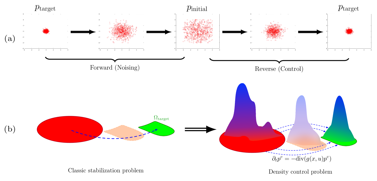
Figure 1: (a) DDPMs in two dimensions, transforming the data distribution $p_{\text{target}}$ to $p_{n}$ and learning to reverse the process. (b) Reformulation from the classical control problem to the density control problem.

We now formally state the DDPM based feedback control problem. Toward this end, we will need a description of how the density of the solution $x$ of equation (1). This is known to be given by the Liouville equation or the continuity equation [32],

$$\partial_{t}p^{\textup{c}}=-\textup{div}(g(x,\pi(t,x))p^{\textup{c}}),$$ (10)

for a given initial density $p^{\textup{c}}_{0}=p_{0}$.

In terms of the above equation, our goal is to design a control policy $\pi(t,x)$ such that $p_{T}=p_{d}$. In the DDPM based control methodology we will construct a stochastic process with probability density $p^{f}_{t}$ such that $p^{f}_{T}\approx p_{0}$ and $p^{f}_{0}=p_{d}$.

We will consider two instances of the DDPM based control problem where the probability distribution $p^{f}$ corresponds to the evolution of the corresponding forward process:

1. Algorithm 1: The forward process $X^{f}$ follows a stochastic differential equation (SDE) of the form:

   $$\textup{d}X^{\text{f}}=V(X^{\text{f}})+\sqrt{2}\,\textup{d}W+\textup{d}Z,$$ (11)

2. Algorithm 2: The forward process evolves according to a controlled dynamical system with diffusion,

   $$dX^{f}= -g_{0}(X^{f})+\sum_{i}^{m}v_{i}(X^{f})g_{i}(X^{f})$$ (12)

   $$+\sqrt{2}\sum_{i}^{m}g_{i}(X^{f})\odot dW+\textup{d}Z.$$

In each instance, the problem we will be interested in is the following.

Problem II.1.

(Existence of time reversing control law) Does there exist of a wellposed feedback control policy $u=\pi(t,x)$, such that the density of the controlled state satisfies $p^{\textup{c}}_{t}=p^{\textup{f}}_{T-t}$ for all $t\in[0,T]$? If yes, identify such a feedback control policy $\pi(t,x)$.

Classical results on time reversal of diffusion processes [33, 34, 35] establish conditions under which the reverse process of a stochastic system can be realized. A significant challenge addressed by these works is that the coefficients of the time-reversing coefficients are not globally Lipschitz. Hence, one cannot use classical existence-uniqueness criteria to construct the reverse process over the time horizon. We seek to address a similar challenge of time reversal in our work. However, our work differs in two fundamental ways:

• The reverse process in our setting is deterministic, which is crucial for control applications where injecting noise into the system is undesirable.

• Unlike prior work that assumes the noise and control channels are the same, we relax this assumption for systems without drift.

We will say that there exists a deterministic realization associated with the control $\pi(t,x)$ if there exists a probability measure $\mathbb{P}$ on $C([0,T];\mathbb{R}^{d})$ such that

$$\dot{\gamma}_{t}=g_{0}(\gamma_{t})+\sum_{i=1}^{m}\pi(t,\gamma_{t})g_{i}(\gamma_{t}),$$ (13)

for $\mathbb{P}$ almost every $\omega\in C([0,T];\mathbb{R}^{d})$, and $\mathbb{P}(\gamma_{t}\in dx)=p^{f}_{T-t}(x)$, for all $t\in[0,T]$. Given this definition, we will address the following problem.

Problem II.2.

(Deterministic realization of reverse process) Given a solution to Problem II.1, does there exist a deterministic realization of the reverse process?

Before we proceed to the next section, we make a remark connecting the denoising problem to classical control problem. Addressing the above two objectives provides one a way of controlling a system from one probability density to another. If the forward process takes the system from a target probability density to a noise distribution. The time reversing control law then takes the system from the noise distribution to the final distribution. This can be considered as a general version of the classical control problem in which the goal is to design a control law $\pi(t,x)$ such that the state $x$ reaches a target set $\Omega_{\text{target}}$. Reformulating this as a density control problem allows a probabilistic interpretation of stabilization. Let $p_{n}$ be the initial density and $p_{\text{target}}$ the target density. The DDPM control problem consists of designing a policy $\pi(t,x)$ such that the density trajectory satisfies

$$p^{\textup{c}}_{t}=p^{f}_{t-T},\quad p^{f}_{0}=p_{\text{target}}=c\mathbf{1}_{\Omega_{\text{target}}}.$$ (14)

where $c\mathbf{1}_{\Omega_{\text{target}}}$ is the normalized support function of $\Omega_{\text{target}}$ This framework unifies classical and probabilistic stabilization, providing an alternative approach to nonlinear control. Figure 1 illustrates this reformulation.

III Algorithms for DDPM-based control

In this section, we provide details on the two DDPM based algorithms that we will use to solve the DDPM based approach to address the probability density control problem. The first algorithm is expected to approximate the achieve the control objective better due to the choice of the loss function, while second algorithm is computationally more scalable as it transforms the reversing problem into a regression problem.

III-A Algorithm 1

Adapting the methodology introduced in Section II-A, we take (1) to be the reverse process, retaining (2) as the forward process. If we set $V(x)=-\nabla\log p_{n}$, then the forward process provides a reference trajectory $p^{\textup{f}}_{T-t}$ in the set of probability densities such that $p^{\textup{f}}_{T}\approx p_{n}$ and $p_{0}=p_{\text{target}}$. Thus if there exists a controller $\pi(t,x)$ that can ensure system (1) exactly tracks this density trajectory, we will have that $p_{T}^{\textup{c}}\approx p_{\text{target}}$.

To identify the controller $\pi(t,x)$, we seek to the following minimization problem:

$$\min_{\pi}\frac{1}{T}\int\limits_{0}^{T}\text{KL}(p^{\textup{c}}\big{|}p^{\textup{f}}_{T-t})\ \textup{d}t.$$ (15)

subject to the dynamics

$$\partial_{t}p^{\textup{c}}=-\text{div}(g(x,\texttt{NN}(t,x,\theta))p^{\textup{c}}),$$ (16)

where $p^{\textup{c}}_{0}=p_{n}$. Here $\text{KL}(p^{\textup{c}}\big{|}p^{\textup{f}})$ denotes the KL divergence between the density of the control system and the forward density. The KL divergence between any two densities $Q$ and $R$ defined on a set $\Omega$ is given by

$$\text{KL}(Q\big{|}R) =\int\limits_{x\in\Omega}Q(x)\log\left(\frac{Q(x)}{R(x)}\right)~\textup{d}x.$$ (17)

III-B Algorithm 2

A drawback of the previous algorithm is that (15)-(16) is a constrained optimization problem, with constraints (16). This implies that the equation (16) needs to be solved in every pass of the gradient descent. To address this issue, we present an alternative algorithm.

Toward this end, we associate with each vector-field $g_{i}:\mathbb{R}^{d}\rightarrow\mathbb{R}^{d}$ a first order differential operator $Y_{i}$, given by

$$Y_{i}~\cdot=\sum_{j=1}^{d}g^{j}_{i}(x)\partial_{x_{j}}$$

where $Y_{i}^{*}$ is the formal adjoint of the operator $Y_{i}$ and is given by

$$Y_{i}^{*}=\sum_{j=1}^{d}-\frac{\partial}{\partial x_{j}}(g_{i}^{j}~~~\cdot)~~~$$

The operator $Y_{i}^{*}$ is the formal adjoint of $Y_{i}$ can be seen from the computation

$$\int_{\mathbb{R}^{d}}g(x)Y_{i}f(x)dx=\int_{\mathbb{R}^{d}}f(x)Y^{*}_{i}g(x)dx$$

for every smooth compactly supported function $f,g\in C^{\infty}_{c}(\mathbb{R}^{d})$, by applying integration by parts.

Using these operators, the continuity equation (10) can be expressed as

$$\partial_{t}p^{f}=Y^{*}_{0}p^{c}+\sum_{i=1}^{m}Y_{i}^{*}(\pi_{i}(t,x)p^{c})$$ (18)

Forward Process While in the previous algorithm, we retained (2) as the forward process, in this section we take (12) as the forward process. The probability distribution $p^{f}$ of the process 12 evolves according to

$$\partial_{t}p^{f}=-Y^{*}_{0}p^{f}+\sum_{i=1}^{m}(Y_{i}^{*})^{2}p^{f}+\sum_{i=1}^{m}Y_{i}^{*}(v_{i}(x)p^{f})$$ (19)

First, an important requirement for the forward process is that it has the equilibrium distribution $p_{n}$. For this purpose, we need to control the long term behavior of the probability distribution of the forward process (12).

We will assume that we can construct control laws $v_{i}(x)$, such that above PDE can be transformed to the form,

$$\partial_{t}p^{f}=-Y^{*}_{0}p^{f}-\sum_{i=1}^{m}Y_{i}^{*}Y_{i}p^{f}+\sum_{i=1}^{m}Y_{i}^{*}(w_{i}(x)p^{f})$$ (20)

for some choice of $w_{i}(x)$, so that $p_{n}$ is it’s equilibrium solution. We will show in Section IV-A that for each $p_{n}$ such a choice of $v_{i}(x)$ and $w_{i}(x)$ always exists, whenever the system is driftless. When the system is a linear time invariant system, one can choose $p_{n}$ from a class of Gaussian distributions by setting $w_{i}(x)\equiv 0$.

We can rewrite this equation in the form

$$\partial_{t}p^{f} =-Y_{0}p^{f}-\sum_{i=1}^{m}Y_{i}^{*}\left(\dfrac{Y_{i}p^{f}}{p^{f}}\right)p^{f}+\sum_{i=1}^{m}Y_{i}^{*}(w_{i}(x)p^{f})$$ (21)

Therefore, we have Nonholonomic score loss. This gives us the nonholonomic score matching objective where we want to approximate the nonholonomic score $\frac{Y_{i}p^{f}}{p^{f}}$ using the neural network $s^{\theta}_{i}(t,x)$

$$\min_{\theta}\int_{0}^{T}\int_{\mathbb{R}^{d}}\|s^{\theta}(t,x)-\nabla_{c}\log p^{f}_{t}(x)\|^{2}p^{f}_{T-t}(x)dx$$ (22)

where $\nabla_{c}$ is nonholonomic gradient operator defined by

$$\nabla_{c}f =[Y_{1}f,...,Y_{m}f]^{T}$$

$$=[\sum_{j=1}^{d}g^{j}_{1}(x)\partial_{x_{j}}f(x),...,\sum_{j=1}^{d}g^{j}_{m}(x)\partial_{x_{j}}f(x)]^{T}$$ (23)

If we use the exact score $\nabla_{c}\log p^{f}_{T-t}$ to execute the control $\pi(t,x)=\nabla_{c}\log p^{f}_{T-t}-v(x)$ in the reverse process (1) and $p^{c}\approx p^{f}_{T}$, then substituting in equation we get that $p^{c}_{t}=p^{f}_{T-t}$ for all $t\in[0,T]$ and the continuity equation (18) becomes

$$\partial_{t}p^{c}=Y^{*}_{0}p^{c}+\sum_{i=1}^{m}Y_{i}^{*}(\frac{Y_{i}p^{f}_{T-t}}{p^{f}_{T-t}}p^{c})-\sum_{i=1}^{m}Y_{i}^{*}(w_{i}(x)p^{c})$$ (24)

IV Analysis

The primary objective of this section is to establish a rigorous mathematical foundation for the deterministic realization of diffusion-based control processes (Problems II.1 and II.2). For each algorithm presented in the previous section, we will proceed with the analysis in with the following steps :

1. Step 1: Mathematical Preliminaries – We introduce key concepts from geometric control theory and PDE theory, including weak solutions to the Fokker-Planck equation and the continuity equation, as well as proofs of regularity for PDEs that arise in the evolution of probability densities under controlled dynamics.

2. Step 2: Time Reversal and Existence Conditions – Using the regularity results, we establish conditions under which a deterministic feedback law can enforce time-reversed evolution of probability densities. Specifically, we analyze whether the controlled evolution of the system state can replicate the reverse-time dynamics of a diffusion process.

3. Step 3: Application to Linear and Drift-Free Systems – We prove results that ensure the existence of valid control laws in both driftless nonlinear systems and linear time-invariant (LTI) systems, demonstrating how deterministic control can be leveraged for state density evolution in these structured settings.

IV-A Analysis of Algorithm 1 (Driftless Systems)

We address the well-posedness of problem (15) from a theoretical point of view. The nonlinear dynamics of system (1) play a crucial role in the feasibility of this problem. In typical DDPM problems for generative modeling, noise can be added in all directions for both the forward and reverse processes. Therefore, score-matching techniques can be employed to learn the reverse process. However, for the feedback control problem in consideration, if the dynamical system is not fully actuated, that is $d=m$, then the feasibility of problem (15) is not clear. Here, we address the case when such a controller can be obtained.

Let $\mathcal{V}=\{g_{0},g_{1},...,g_{m}\}$, $m\leq d$, be a collection of smooth vector fields $g_{i}:\mathbb{R}^{d}\rightarrow\mathbb{R}^{d}$. Let $[f,g]$ denote the Lie bracket operation between two vector fields $f:\mathbb{R}^{d}\rightarrow\mathbb{R}^{d}$ and $g:\mathbb{R}^{d}\rightarrow\mathbb{R}^{d}$, given by where $\partial_{i}$ denotes partial derivative with respect to coordinate $i$.

$$[f,g]_{i}=\sum_{j=1}^{d}f^{j}\partial_{x_{j}}g^{i}-g^{j}\partial_{x_{j}}f^{i}.$$ (25)

We define $\mathcal{V}^{0}=\mathcal{V}$. For each $i\in\mathbb{Z}_{+}$, we define in an iterative manner the set of vector fields $\mathcal{V}^{i}=\{[g,h];~g\in\mathcal{V},~h\in\mathcal{V}^{j-1},~j=1,...,i\}$. We will assume that the collection of vector fields $\mathcal{V}$ satisfies following condition the Chow-Rashevsky condition [36] (also known as Hörmander’s condition [37]). For the purposes of this section, we will need the following assumption.

Assumption IV.1.

(Controllable driftless system) There is no drift in the system ($g\equiv 0$). The Lie algebra generated by the vector fields $\mathcal{V}$, given by $\cup_{i=0}^{r}\mathcal{V}^{i}$, has rank $N$, for sufficiently large $r$.

We will need another assumption on the regularity of $\Omega$. Towards this end an admissible curve $\gamma:[0,1]\rightarrow\Omega$ connecting two points $x,y\in\Omega$ is a Lipschitz curve in $\Omega$ for which there exist essentially bounded functions $u_{i}:[0,T]\rightarrow\mathbb{R}$ such that $\gamma$ is a solution of (1) with $\gamma(0)=x$ and $\gamma(1)=y$.

Definition IV.2.

The domain $\Omega\subset\mathbb{R}^{d}$ is said to be non-characteristic if for every $x\in\partial\Omega$, there exists a admissible curve $\gamma(t)$ such $\gamma(0)=x$ and $\gamma(t)$ is not tangential to $\partial\Omega$ at $x$.

This definition imposes a regularity on the domain $\Omega$, which will be needed to apply the results of [25] to conclude the invertibility of the operator $\sum_{i=1}^{m}Y_{i}^{*}Y_{i}$.

Assumption IV.3.

(Compact Domain) In the compact case, we will make the following assumptions on the boundary of the domain $\Omega$.

1. The domain $\Omega$ is compact and has a $C^{2}$ boundary $\partial\Omega$.

2. The domain $\Omega$ is non-characteristic in the sense of Definition IV.2.

Assumption IV.4.

(Smoothness of Density) The densities $p_{\rm target},p_{n}\in C^{\infty}({\Omega})$ and strictly positive on ${\Omega}$.

We will say that $p\in L^{2}(\Omega)$ is a probability density, if $\int_{\Omega}p(x)dx=1$ and $p$ is non-negative almost everywhere on $\Omega$.

Given these definitions we will show that we can a find a feedback controller $u_{i}=\pi_{i}(t,x)$ such that the dynamical system tracks the forward process in reverse.

In order to state our main result, we will need to define some mathematical notions that will be used in this section. We define $L^{2}(\Omega)$ as the space of square integrable functions over $\Omega$, where $\Omega\subset\mathbb{R}^{d}$ is an open, bounded and connected subset. The set of continuous functions $p$ for which $p_{t}$ lies in a Hilbert space $X$ will be referred to using $C([0,1];X)$.

For a given real-valued function $a\in L^{\infty}(\Omega)$, $L^{2}_{a}(\Omega)$ refers to the set of all functions $f$ such that the norm of $f$ is defined as $\|f\|_{a}:=(\int_{\Omega}|f(x)|^{2}a(x)dx)^{{1/2}}<\infty.$ We will always assume that the associated function $a$ is uniformly bounded from below by a positive constant, in which case the space $L^{2}_{a}(\Omega)$ is a Hilbert space with respect to the weighted inner product $\langle\cdot,\cdot\rangle_{a}:L^{2}_{a}(\Omega)\times L^{2}_{a}(\Omega)\rightarrow\mathbb{R}$, given by $\langle f,g\rangle_{a}=\int_{\Omega}f(x){g}(x)a(x)dx$ for each $f,g\in L^{2}_{a}(\Omega)$. When $a=\mathbf{1}$, where $\mathbf{1}$ is the function that takes the value $1$ almost everywhere on $\Omega$, the space $L^{2}_{a}(\Omega)$ coincides with the space $L^{2}(\Omega)$. Due to the assumptions on $a$, the spaces $L^{2}(\Omega)$ and $L^{2}_{a}(\Omega)$ are isomorphic and the same is true for the spaces $C([0,T];L^{2}(\Omega)$ and $C([0,T];L^{2}_{a}(\Omega)$. We will use this fact repeatedly. For a function $f\in L^{2}(\Omega)$ and a given constant $c$, we write $f\geq c$ to imply that $f$ is real-valued and $f(x)\geq c$ for almost every (a.e.) $x\in\Omega$. Let $L^{2}_{a,\perp}(\Omega):=\{f\in L^{2}_{a}(\Omega);\int_{\Omega}f(x)dx=0\}$ be the subspace of functions in $L^{2}_{a}(\Omega)$ that integrate to $0$.

We define the weighted horizontal Sobolev space $WH^{1}_{a}(\Omega)=\big{\{}f\in L^{2}(\Omega):Y_{i}(af)\in L^{2}(\Omega)\text{ for }1\leq i\leq m\big{\}}$. We equip this space with the weighted horizontal Sobolev norm $\|\cdot\|_{WH^{1}_{a}}$, given by $\|f\|_{WH^{1}_{a}}=\Big{(}\|f\|^{2}_{2}+\sum_{i=1}^{n}\|Y_{i}(af)\|^{2}_{2}\Big{)}^{1/2}$ for each $f\in WH^{1}_{a}(\Omega)$. Here, the derivative action of $Y_{i}$ on a function $f$ is to be understood in the distributional sense. When $a=\mathbf{1}$, where $\mathbf{1}$ is the constant function that is equal to $1$ everywhere, we will denote $WH_{a}^{1}(\Omega)$ by $WH^{1}(\Omega)$.

Before we present our stability analysis, we give some more preliminary definitions. Given $a\in L^{\infty}(\Omega)$ such that $a\geq c$ for some positive constant $c$, and $\mathcal{D}(\omega_{a})=WH^{1}_{a}(\Omega)$, we define the sesquilinear form $\omega_{a}:\mathcal{D}(\omega_{a})\times\mathcal{D}(\omega_{a})\rightarrow\mathbb{R}$ as

$$\omega_{a}(u,v)=\sum\limits_{i=1}^{m}\int\limits_{\Omega}\frac{1}{a(x)}Y_{i}(a(x)u(x))\cdot Y_{i}(a(x){v}(x))dx$$

for each $u\in\mathcal{D}(\omega_{a})$. We associate with the form $\omega_{a}$ an operator $\mathcal{A}^{a}:\mathcal{D}(\mathcal{A}^{a})\rightarrow L^{2}_{a}(\Omega)$, defined as $\mathcal{A}^{a}u=f$, if $\omega_{a}(u,v)=\langle f,v\rangle_{a}$ for all $v\in\mathcal{D}(\omega_{a})$ and for all $u\in\mathcal{D}(\mathcal{A}^{a})=\{g\in\mathcal{D}(\omega_{a}):~\exists f\in L^{2}_{a}(\Omega)~\text{s.t.}~\omega_{a}(g,v)=\langle f,v\rangle_{a}~\forall v\in\mathcal{D}(\omega_{a})\}$. The operator $\mathcal{A}^{a}=-\sum_{i=1}Y_{i}^{*}(\frac{1}{a(x)}Y_{i}(a(x)\cdot))$. We will use an alternative expression of the operator that will be useful in the computations later, and also connect to the operator classical Fokker-Planck operators.

We wish to express the operator $\mathcal{A}^{a}$ in a form similar to the well known Fokker-Plack operator $\Delta u=\nabla\cdot(V(x)u)$. Toward this end, Let $\mathcal{A}^{a}u=f$. If $a=\frac{1}{p_{n}}$ is the noise distribution, by Green’s theorem we get,

$$\omega_{a}(u,v)$$

$$=\sum_{i=1}^{m}\int_{\Omega}p_{n}(x)Y_{i}\left(\frac{u(x)}{p_{n}(x)}\right)\cdot Y_{i}\left(\frac{v(x)}{p_{n}(x)}\right)\,dx$$

$$=-\sum_{i=1}^{m}\int_{\Omega}Y_{i}^{*}\left(p_{n}(x)Y_{i}\left(\frac{u(x)}{p_{n}(x)}\right)\right)\cdot\frac{v(x)}{p_{n}(x)}\,dx$$

$$\quad+\sum_{i=1}^{m}\int_{\partial\Omega}\vec{n}\cdot\left(g_{i}Y_{i}\left(\frac{v(x)}{p_{n}(x)}\right)\right)\frac{v(x)}{p_{n}(x)}\,dS$$

$$=-\sum_{i=1}^{m}\int_{\Omega}Y_{i}^{*}\left(\frac{p_{n}(x)Y_{i}u(x)-u(x)Y_{i}p_{n}(x)}{p_{n}(x)}\right)\cdot\frac{v(x)}{p_{n}(x)}\,dx$$

$$\quad+\sum_{i=1}^{m}\int_{\partial\Omega}\vec{n}\cdot\left(g_{i}Y_{i}\left(\frac{v(x)}{p_{n}(x)}\right)\right)\frac{v(x)}{p_{n}(x)}\,dS$$

$$=-\sum_{i=1}^{m}\int_{\Omega}\left(Y_{i}^{*}Y_{i}u(x)-\frac{u(x)Y_{i}p_{n}(x)}{p_{n}(x)}\right)\cdot\frac{v(x)}{p_{n}(x)}\,dx$$

$$\quad+\sum_{i=1}^{m}\int_{\partial\Omega}\vec{n}\cdot\left(g_{i}Y_{i}\left(\frac{u(x)}{p_{n}(x)}\right)\right)\frac{v(x)}{p_{n}(x)}\,dS$$

$$=\langle\mathcal{A}^{a}u,v\rangle_{a}=\langle f,v\rangle_{a}$$

for all $v\in WH^{a}(\Omega)$. The last expression must hold for all $v$. Therefore, formally, we can conclude that $u$ satisfies the boundary condition,

$$\sum_{i=1}^{m}\vec{n}\cdot(g_{i}Y_{i}(\frac{u}{p_{n}(x)}))=0$$ (26)

Therefore, the PDE

$$\partial_{t}p=-\sum_{i=1}^{m}Y_{i}^{*}Y_{i}p+\sum_{i=1}^{m}Y_{i}^{*}(p\frac{Y_{i}p_{n}}{p_{n}})~~in~~\Omega\times[0,T],$$ (27)

with zero flux boundary condition

$$\sum_{i=1}^{m}\vec{n}\cdot(g_{i}Y_{i}(\frac{p}{p_{n}}))=0$$ (28)

can expressed as an abstract ODE given by

$$\dot{p}=\mathcal{A}^{a}p$$ (29)

When $Y_{i}=\partial_{x_{i}}$ are coordinate vector-fields, the operator $\mathcal{A}^{a}$ is becomes the usual Fokker-Planck operator

$$\Delta-\nabla\cdot(\nabla\log p_{n}~~)=\Delta-\nabla\cdot(\frac{\nabla p_{n}}{p_{n}}),$$

and for this special case we will denote the operator by $\mathcal{B}$.

We will need some different notions of solutions for the analysis further ahead. We will say that $p\in C([0,T];L^{2}_{a}(\Omega))$ is a mild solution to (27) if

$$p_{t}=p_{0}-\mathcal{A}^{a}\int_{0}^{t}p_{s}ds$$

for all $t\in(0,T]$. Let $\pi:[0,T]\times\mathbb{R}^{d}\rightarrow\mathbb{R}^{m}$ be a control law.

We will say that $p^{c}_{t}$ is a classical solution of (10) if $p^{c}_{t}\in C^{1}((0,T]\times\mathbb{R}^{d})$ if (10) holds pointwise. Many times, we will need a weaker notion of solutions for this equation. Toward this end, we will say that that $p^{c}_{t}$ is a weak solution to (10) if

$$\int_{0}^{1}\int_{\mathbb{R}^{d}}\big{(}\partial_{t}\phi(t,x)+g(x,\pi(t,x))\cdot\nabla_{x}\phi(t,x)\big{)}p^{c}_{t}(x)dxdt=0$$ (30)

for all $\phi\in C^{\infty}_{c}(\mathbb{R}^{d}\times(0,T))$.

Given these definitions, we note the following properties of the Nonholonomic Fokker-Planck equation (NFE) (27). A majority of the proofs of the properties have been shown in [25]. A brief proof of the statement 3 of the proposition has been provided in the Appendix.

Proposition IV.5 (Properties of the Nonholonomic Fokker-Planck equations).

Let $a=\frac{1}{p_{n}}$ for some function $p_{n}\in L^{\infty}(\Omega)$ such that $a\in L^{\infty}(\Omega)$. Given Assumption IV.3, let $p_{0}\in L^{2}_{a}(\Omega)$, then there exists a (mild) solution $p_{t}\in C([0,T];L^{2}_{a}(\Omega))$ to the Fokker-Planck equation (27). Moreover, the solution satisfies the following properties.

1. There exists a semigroup of operators $(\mathcal{T}(t))_{t\geq 0}$ such that the solution of the (3) is given by $\mathcal{T}(t)p_{0}$.

2. $p_{t}=\mathcal{T}(t)p_{0}\in\mathcal{D}(\mathcal{A}^{a})$ for all $t\in(0,T]$.

3. If $p_{0}\in\mathcal{D}(\mathcal{A}^{a})$, then $\dot{p}=-\mathcal{A}^{a}p$ for all $t\in[0,T]$, and $\dot{p}\in C((0,T];L^{2}_{a}(\Omega))$.

4. The asymptotic stability estimate holds

   $$\|\mathcal{T}(t)-p_{n}\|_{a}\leq Me^{-\omega t}\|p_{0}-p_{n}\|_{a}$$ (31)

   for all $t\geq 0$, for some $M,\omega>0$ independent of $p_{0}$.

In the following proposition we establish the invertibility of the operator $\mathcal{A}^{a}$, which will play an important role in addressing Problem II.1.

Proposition IV.6.

Given Assumption IV.1 and IV.3, Suppose $f\in L^{2}_{a}(\Omega)$ such that $\int_{\Omega}f(x)dx=0$. Then there exists a unique solution $\psi\in WH^{1}_{a}(\Omega)$ to the weighted nonholonomic Poisson equation,

$$\mathcal{A}^{a}\psi=-\sum_{i=1}^{m}Y_{i}^{*}(\frac{1}{a(x)}Y_{i}(a(x)\psi)=f.$$ (32)

Hence, the restriction of the operator $\mathcal{A}^{a}$ on $L^{2}_{{a,\perp}}(\Omega)$, is invertible. Moreover, there exists a constant $C>0$ such that

$$\|Y_{i}(a\psi)\|_{a}\leq C\|f\|_{a}$$ (33)

for all $f\in L^{2}_{{a,\perp}}(\Omega)$.

Proof.

It is easy to see that $1/a$ is an eigenvector of $\mathcal{A}^{a}$ since $Y_{i}(a/a)=Y_{i}\mathbf{1}=\mathbf{0}$. We know [25] from that $1/a$ is an eigenvector with $0$ simple eigenvalue. Moreover, since the domain $\Omega$ satisfies Assumption IV.3 the domain is also NTA [38][Theorem 1.1], and hence also $\epsilon-\delta$ in the sense of [39]. Therefore, from [25][Lemma III.3], the spectrum of $\mathcal{A}^{a}$ is purely discrete, consisting only of eigenvalues of finite multiplicity and have no finite accumulation point. Let $(\lambda_{n})_{n=1}^{\infty}$ be the eigenvalues corresponding to the orthogonal basis of eigenvectors $\{e_{n};n\in\mathbb{N}\}$.

Since the operator $\mathcal{A}^{a}$ is positive and self-adjoint the eigenvalues are ordered in the form $0=\lambda_{1}<\lambda_{2}....$, with $\lim_{n\rightarrow\infty}\lambda_{n}=+\infty$.

Let $u\in L^{2}_{a,\perp}(\Omega)$. Then $u=\sum_{n=2}^{\infty}\alpha_{n}e_{n}$ for some unique sequence $(\alpha_{n})_{n=1}^{\infty}$ such that $\sum_{n=2}^{\infty}|\alpha_{n}|^{2}=\|u\|^{2}_{a}$. From this we can compute that

$$\langle\mathcal{A}^{a}u,u\rangle_{a}=\sum_{n=2}^{\infty}\lambda_{i}|\alpha_{n}|^{2}\geq\frac{1}{\lambda_{2}}\sum_{n=2}^{\infty}|\alpha_{n}|^{2}=\frac{1}{\lambda_{2}}\|u\|^{2}_{2}$$ (34)

Define the space $WH^{1}_{{a,\perp}}(\Omega):=WH^{1}_{a}(\Omega)\cap L^{2}_{{a,\perp}}(\Omega)$ equiped with the norm $\|u\|_{\omega}:=\sqrt{\omega(u,u)}$.

The solvability of equation (32) is equivalent to finding a solution $\psi\in WH^{1}_{{a,\perp}}(\Omega)$ such that

$$\omega_{a}(\psi,v)=<f,v>_{a},~~~\forall v\in\mathcal{D}(\omega)$$

It is easy to see that

$$\omega(u,v)\leq\|u\|_{\omega}\|v\|_{\omega}$$

for all $u,v\in WH^{1}_{{a,\perp}}(\Omega)$ Moreover, from the (Poincare inequality) estimate (34) it follows that that

$$\omega_{a}(u,u)\geq\frac{1}{\lambda_{2}}\|u\|_{a}$$

for all $u\in WH^{1}_{{a,\perp}}(\Omega)$. Hence, existence and uniqueness of the solution $\psi\in WH^{1}_{{a,\perp}}(\Omega)$ follows from the Lax-Milgram theorem [40]. ∎

Using the above result on invertibility of the operator $\mathcal{A}^{a}$, we can establish that that any sufficiently regular trajectory on the set of probability densities can be tracked using the control system in reverse. Using these results, we provide some analysis justifying the use of Algorithm 1.

First, we state a general result that given any curve on the set of probability densities, for controllable driftless systems, one can find a control that exactly tracks the curve.

Lemma IV.7 (Exact tracking of positive densities).

Given Assumption IV.1 and IV.3, suppose $p^{\text{ref}}\in C([0,T];L^{2}(\Omega))$, $\dot{p}^{\text{ref}}\in C([0,T];L^{2}(\Omega))$, $p^{\text{ref}}_{t}$ is a probability density and $p^{ref}_{t}>0$, for all $t\geq 0$. Then there exists a control law $\pi$ of the form

$$\pi_{i}=\frac{Y_{i}(\mathcal{A}^{1})^{-1}\dot{p}^{ref}_{t}}{p^{ref}_{t}}$$

for all $t\in[0,T]$ and a weak solution $p^{\textup{c}}$ of (10) satisfies

$$p^{\textup{c}}_{t}=p^{\text{ref}}_{t}\text{ for all }t\in[0,T]$$

Proof of Lemma IV.7. Let $\psi_{t}=(\mathcal{A}^{1})^{-1}\dot{p}^{ref}_{t}$, for all $t\in[0,T]$. Then the control law law $\pi_{i}(t,x)=\frac{Y_{i}\psi_{t}(x)}{p^{ref}_{t}(x)}$ is well defined by Proposition IV.6.

Let $\phi\in C^{\infty}_{c}((0,T);\mathbb{R}^{d})$. We compute

$$\int_{0}^{T}\int_{\mathbb{R}^{d}}\big{(}\partial_{t}\phi(t,x)+g(x,\pi(t,x))\cdot\nabla_{x}\phi(t,x)\big{)}p^{ref}_{t}(x)dxdt$$

by substituting for $g$ this expression is equivalent to,

$$\int_{0}^{T}\int_{\mathbb{R}^{d}}\big{(}\partial_{t}\phi(t,x)-\sum_{i=1}^{m}\pi_{t}(t,x)\cdot Y_{i}\phi(t,x)\big{)}p^{ref}_{t}(x)dxdt$$

Substituting for the form of the control law we get,

$$\int_{0}^{T}\int_{\mathbb{R}^{d}}\big{(}\partial_{t}\phi(t,x)-\sum_{i=1}\frac{Y_{i}(\mathcal{A}^{1})^{-1}\dot{p}^{ref}}{p^{ref}_{t}}\cdot Y_{i}\phi(t,x)\big{)}p^{ref}_{t}(x)dxdt$$

Since $\sum_{i=1}^{m}Y^{*}_{i}Y_{i}=\mathcal{A}^{1}$, this becomes

$$\int_{0}^{T}\int_{\mathbb{R}^{d}}\big{(}\partial_{t}\phi(t,x)p^{ref}_{t}(x)+\dot{p}^{ref}_{t}\phi(t,x))dxdt$$

By integration by parts with respect to time, and using the fact that $\phi$ is compactly supported, this term is equal to $0$. This concludes that $p^{ref}_{t}$ satisfies the continuity equation.

∎

Given the general result on tracking of probability densities, we can track a forward process in the reverse direction. This is the subject of the following Lemma, which addresses Problem II.1 for Algorithm 1.

Lemma IV.8 (Tracking the Holonomic Fokker-Planck Equation).

Given Assumption IV.3, suppose $p_{0}\in L^{2}(\Omega)$. Let $p^{f}$ be the mild solution of (27) for $\mathcal{A}^{a}=\mathcal{B}^{a}$, then there exists a control law $\pi:[0,T]\times\mathbb{R}^{d}\rightarrow\mathbb{R}^{m}$ of the form

$$\pi_{i}(t,\cdot)=\frac{Y_{i}(\mathcal{A}^{1})^{-1}\dot{p}^{f}_{T-t}}{p^{f}_{T-t}}$$

such that a weak solution $p^{\textup{c}}$ of the (10) satisfies

$$p^{\textup{c}}_{t}=p^{\textup{f}}_{T-t}\text{ for all }t\in[0,T]$$

Proof.

It is a well known property of the solutions of the Fokker-Planck equation that $p^{f}_{t}>0$ for all $t\in(0,T]$. Moreover, $p^{f}_{t}\in\mathcal{D}(\mathcal{B}^{a})$ and we know that $\dot{p}^{f}_{t}=-\mathcal{B}^{a}p^{f}_{t}$ for all $(0,T]$ from Proposition IV.5. This implies that $\langle\mathbf{1},\dot{p}^{f}_{t}\rangle_{2}=\langle\mathcal{B}^{a}\mathbf{1},\dot{p}^{f}_{t}\rangle_{2}=\mathbf{0}$. Hence, $\dot{p}^{f}_{t}\in L^{2}_{{a,\perp}}(\Omega)$ for all $t\in[0,T]$. Additionally, we know from Proposition IV.5 that $\dot{p}^{f}_{t}\in C((0,T];L^{2}_{a}(\Omega))$. ∎

The goal of the next result is to address Problem (II.2) for Algorithm 2. The idea is that in general, we do not know if the the vector field generated by the time-reversing control laws are Lipschitz. Hence, one cannot construct a probability measure by using the flow map associated with the vector-field. Nevertheless, the following result from optimal transport theory [41] enables the construction of such a measure.

Theorem IV.9.

([41]) (Superposition solution) Let $t\mapsto\mu_{t}\in\mathcal{P}(\mathbb{R}^{d})$ be such that $\mu_{t}$ is a weak solution to the continuity equation according to (30) and

$$\int_{0}^{T}\int_{\mathbb{R}^{d}}\frac{|v(t,x)|}{1+|x|}d\mu_{t}(x)dt<\infty$$

Then there exist a probability measure $\mathbb{P}\in\mathcal{P}(\mathbb{R}^{d}\times C([0,T];\mathbb{R}^{d}))$ such that

$$\dot{\gamma}(t)=v(t,\gamma(t)),~~\gamma(0)=y$$ (35)

for $\mathbb{P}$ almost every $(y,\gamma)\in\mathbb{R}^{d}\times C([0,T];\mathbb{R}^{d})$, and $\mathbb{P}(\gamma_{t}\in dx)=d\mu_{t}(x)$, for all $t\in[0,T]$.

Given this result we can construct a deterministic realization to the reverse process, as show in the following theorem. A key factor that helps us to verify the integrability requirement of the vector field is the regularity of the control law, which is due to the regularity of the solution of the inverses of Poisson equation as established in Proposition IV.6.

Theorem IV.10.

(Determinsitic realization of reverse process) Given Assumption IV.3. Suppose $p_{0}\in L^{2}(\Omega)$ is a probability density. Let $\pi_{i}$ be the control law given by

$$\pi_{i}(\cdot,t)=\frac{Y_{i}\mathcal{A}^{-1}\dot{p}^{c}}{p^{c}_{t}}$$

for all $t\in(T,0]$ such that a weak solution $p^{\textup{c}}$ of the (LABEL:eq:ctctty) satisfies

$$p^{\textup{c}}_{t}=p^{\textup{f}}_{T-t}\text{ for all }t\in[0,T]$$

as shown by Lemma IV.8. Then for every $\epsilon$ there exists a probability measure $\mathbb{P}\in\mathcal{P}(\mathbb{R}^{d}\times C([0,T-\epsilon];\mathbb{R}^{d}))$ such that

$$\dot{\gamma}_{t}=\sum_{i=1}^{m}\pi_{i}(t,\gamma_{t})g_{i}(\gamma_{t}),~~\gamma(0)=y$$ (36)

for $\mathbb{P}$ almost every $(y,\gamma)\in\mathbb{R}^{d}\times C([0,T];\mathbb{R}^{d}),$ for all $t\in[0,T]$ and, $\mathbb{P}(\gamma_{t}\in dx)=p^{c}_{t}(x)dx$, for all $t\in[0,T]$.

Moreover, if $p_{0}\in\mathcal{D}(\mathcal{B}^{1})$, then we can take $\epsilon=0$.

Proof.

We compute,

$$\int_{0}^{T-\epsilon}\int_{\mathbb{R}^{d}}|\pi_{i}(t,x)|p^{c}_{t}(x)dxdt$$

$$=\int_{0}^{T-\epsilon}\int_{\mathbb{R}^{d}}|\frac{Y_{i}\mathcal{A}^{-1}\dot{p}^{c}}{p^{c}_{t}}|p^{c}_{t}(x)|dxdt$$

$$=\int_{0}^{T-\epsilon}\int_{\mathbb{R}^{d}}|Y_{i}\mathcal{A}^{-1}\dot{p}^{c}_{t}(x)|dxdt$$

Since, $\dot{p}^{f}_{t}\in C(0,T];L^{2}(\Omega))$ and hence $\dot{p}^{c}_{t}\in C[0,T);L^{2}(\Omega))$ by IV.6, we can conclude that this term is bounded for every $\epsilon>0$. Since the vector-fields $g_{i}$ are bounded on a compact set this implies that for $v(t,x)=\sum_{i=1}^{m}\pi_{i}(t,x)g_{i}(x)$

$$\int_{0}^{T-\epsilon}\int_{\mathbb{R}^{d}}\frac{|v(t,x)|}{1+|x|}d\mu_{t}(x)dt<\infty.$$

Therefore, the existence of superposition solutions follows from IV.9. If $p_{0}\in\mathcal{D}(\mathcal{B}^{1})$, then we can see that the integral estimate holds for $\epsilon=0$, since in this case we have $\dot{p^{c}_{t}}\in C([0,T];L^{2}(\Omega))$. Therefore, $\int_{\mathbb{R}^{d}}|Y_{i}\mathcal{A}^{-1}\dot{p}^{c}_{t}(x)|$ is uniformly bounded over $[0,T]$. ∎

IV-B Analysis of Algorithm 2 (Score Matching)

In this section, we analyze the score matching approach used in Algorithm 2. In this case, we consider two different cases. When the system is driftless and the case of linear time invariant systems. Since, the case of the linear time invariant system comes with some restrictions in terms of the kind of noise distributions that one can converge to in the forward process, we consider these two cases separately.

IV-B1 Driftless Systems

In the first result, we derive what are the class of noise distributions that one can drive the forward process to asymptotcally and construct a closed form solution of the feedback control laws.

Theorem IV.11.

(Convergence of driftless system to noise distribution) Suppose the system (1) is driftless. That is $X_{0}\equiv 0$. Then for the choice of control law

$$v_{i}=\sum_{j=1}^{n}\frac{\partial g_{i}^{j}}{\partial x_{j}}+\frac{Y_{i}p_{n}}{p_{n}}$$ (37)

the evolution of the probability density (19) is equivalently described by the equation

$$\partial_{t}p=-\sum_{i=1}^{m}Y_{i}^{*}Y_{i}p+\sum_{i=1}^{m}Y_{i}^{*}(p\frac{Y_{i}p_{n}}{p_{n}})$$ (38)

Consequently, for the zero flux boundary condition (28), given $p_{0}\in L^{2}(\Omega)\cap\mathcal{P}(\Omega)$, there exist constants $M>0$ and $\lambda>0$ such that the solution of (46) satisfies

$$\|p_{t}-p_{n}\|_{2}\leq Me^{-\lambda t}\|p_{0}-p_{n}\|_{2}$$ (39)

for all $t\geq 0$.

Proof.

Suppose the system (1) is driftless, i.e., $X_{0}\equiv 0$. Then, for the choice of control law

$$v_{i}=\sum_{j=1}^{n}\frac{\partial g_{i}^{j}}{\partial x_{j}}+\frac{Y_{i}p_{n}}{p_{n}},$$ (40)

the evolution of the probability density (19) is equivalently described by the equation

$$\partial_{t}p=\sum_{i=1}^{m}Y_{i}^{*}Y_{i}p-\sum_{i=1}^{m}Y_{i}^{*}\left(p\frac{Y_{i}p_{n}}{p_{n}}\right).$$ (41)

Consequently, given $p_{0}\in L^{2}(\Omega)\cap\mathcal{P}_{2}(\Omega)$, there exist constants $M>0$ and $\lambda>0$ such that the solution of (46) satisfies

$$\|p_{t}-p_{n}\|_{2}\leq Me^{-\lambda t}\|p_{0}-p_{n}\|_{2}$$ (42)

for all $t\geq 0$. The (mild) solution of this equation is given by the semigroup generated by the operator $-\mathcal{A}^{a}$ for $a=1/p_{n}$. Therefore the exponential stability result follows from IV.5. ∎

Proof.

We require that $v_{i}(x)$ is such that

$$\sum_{i=1}^{m}(Y_{i}^{*})^{2}p+\sum_{i=1}^{m}Y_{i}^{*}(v_{i}(x)p)$$ (43)

$$=\sum_{i=1}^{m}-(Y_{i}^{*}Y_{i})p+\sum_{i=1}^{m}Y_{i}^{*}\left(p\frac{Y_{i}p_{n}}{p_{n}}\right).$$ (44)

Firstly, by the product rule:

$$Y_{i}^{*} =\sum_{j=1}^{n}-\frac{\partial}{\partial x_{j}}\left(g_{i}^{j}\cdot\right)$$

$$=\sum_{j=1}^{n}-\frac{\partial g_{i}^{j}}{\partial x_{j}}\left(\cdot\right)-\sum_{j=1}^{n}g_{i}^{j}\frac{\partial}{\partial x_{j}}\left(\cdot\right)$$

$$=\sum_{j=1}^{n}-\frac{\partial g_{i}^{j}}{\partial x_{j}}\left(\cdot\right)-Y_{i}.$$

Therefore, we have:

$$Y_{i}=\sum_{j=1}^{n}-\frac{\partial g_{i}^{j}}{\partial x_{j}}\left(\cdot\right)-Y_{i}^{*}.$$

If we set

$$v_{i}=\sum_{j=1}^{n}\frac{\partial g_{i}^{j}}{\partial x_{j}}+\frac{Y_{i}p_{n}}{p_{n}},$$

we get:

$$\sum_{i=1}^{m}(Y_{i}^{*})^{2}+\sum_{i=1}^{m}Y_{i}^{*}\left(-Y_{i}-Y_{i}^{*}\right)+\sum_{i=1}^{m}Y_{i}^{*}\left(\cdot\frac{Y_{i}p_{n}}{p_{n}}\right)$$

$$=-\sum_{i=1}^{m}Y_{i}^{*}Y_{i}+\sum_{i=1}^{m}Y_{i}^{*}\left(\cdot\frac{Y_{i}p_{n}}{p_{n}}\right).$$ (45)

Then, equation (19) becomes:

$$\partial_{t}p=-\sum_{i=1}^{m}Y_{i}^{*}Y_{i}p+\sum_{i=1}^{m}Y_{i}^{*}\left(p\frac{Y_{i}p_{n}}{p_{n}}\right).$$ (46)

The (mild) solution to this equation is given by the semigroup generated by the operator $-\mathcal{A}^{a}$ for $a=1/p_{n}$. Hence, the result follows from Proposition IV.5. ∎

In the following theorem we establish that solutions of the nonholonomic Fokker-equation remain positive for all time $t>0$. The semigroup $\mathcal{T}^{\mathcal{A}^{a}}(t)$ generated by the operator $\mathcal{A}^{a}$ is irreducible. That is, if $p_{0}\geq 0$, then $\mathcal{T}^{\mathcal{A}^{a}}(t)p_{0}>0$ for every $t>0$. Since the expression involves the solution $p^{f}_{t}$ in the denominator, this ensures that the time reversing control law computed further ahead is well posed.

Proposition IV.12.

The semigroup $\mathcal{T}^{\mathcal{A}^{a}}(t)$ generated by the operator $\mathcal{A}^{a}$ is irreducible. That is, if $p_{0}\geq 0$, then $\mathcal{T}^{\mathcal{A}^{a}}(t)p_{0}>0$ for every $t>0$.

Proof.

For any any measurable set $\tilde{\Omega}\subseteq\Omega$, let $\xi_{\tilde{\Omega}}$ denote the characteristic function. According to [42, Corollary 2.11] irreducibility of the semigroup is equivalent to the fact that there exists $\Omega_{1}\subset\Omega$ such that the Lebesgue measure of $\Omega\backslash\Omega_{1}$ is not equal to $0$ and whenever $u$ lies in form domain $\mathcal{D}(\omega_{a})$ we also have that $\xi_{\Omega_{1}}u$ lies in the domain of the form $\mathcal{D}(\omega_{a})$. Clearly, $1/a$ lies in the form domain. Suppose the semigroup is not irreducible. Then $v=\xi_{\Omega_{1}}1/a$ must lie in the form domain for some set $\Omega_{1}$. We know that $v\in\mathcal{D}(\omega_{a})$ implies $\xi_{\Omega_{1}}\in\mathcal{D}(\omega_{\mathbf{1}})$. It is a property of weak derivatives that $\xi_{\{v=0\}}Y_{i}v=0$, where $\{v=0\}=:\{x\in\Omega;v(x)=0\}$. This implies that $Y_{i}\xi_{\Omega_{1}}=\xi_{\Omega_{1}}Y_{i}\xi_{\Omega}=\xi_{\Omega_{1}}Y_{i}\mathbf{1}=0$. Therefore, $\omega_{1}(\xi_{\Omega_{1}},\xi_{\Omega_{1}})=0$ and hence $\mathcal{A}^{\mathbf{1}}\xi_{\Omega_{1}}=\mathbf{0}$. This contradicts with [25, Theorem 3.6] that $0$ is a simple eigenvalue of $\mathcal{A}^{\mathbf{1}}$, unless $\Omega_{1}$ has either full Lebesgue measure or 0 Lebesgue measure. ∎

Given this result of irreducibility, we can construct a deterministic control law that realizes the forward process. By reversibility of the continuity equation, this immediately also implies the control law can be used to reverse the forward process.

Proposition IV.13.

Suppose the system is a controllable driftless system on a compact domain. Let $p^{f}_{t}$ be the mild solution of (27). Consider the control law

$$\pi_{i}(t,\cdot)=\frac{Y_{i}p_{n}}{p_{n}}-\frac{Y_{i}p^{f}_{t}}{p^{f}_{t}}$$

Then $p^{f}_{t}$ also solves the continuity equation in the weak sense as in definition (30).

Proof.

The expression is well posed by Proposition IV.12. Let $\phi\in C^{\infty}_{c}((0,T)\times\mathbb{R}^{d})$. By substituting for $\pi_{i}$ in the definition (30), we compute, IV.11,

$$\int_{\mathbb{R}^{d}}\big{(}\partial_{t}\phi(t,x)+(g(x,\pi(t,x)))\cdot\phi(t,x)\big{)}p^{f}_{t}(x)dx$$ (47)

$$=\int_{\mathbb{R}^{d}}\big{(}\partial_{t}\phi(t,x)+\sum_{i=1}^{m}(\pi_{i}(t,x)\cdot Y_{i}\phi(t,x)\big{)}p^{f}_{t}(x)dx$$

$$=\int_{\mathbb{R}^{d}}\partial_{t}\phi(t,x)+\sum_{i}(\frac{Y_{i}p^{f}_{t}}{p^{f}_{t}}-\frac{Y_{i}p_{n}}{p_{n}})\cdot Y_{i}\phi(t,x)\big{)}p^{f}_{t}(x)dx$$

$$=\int_{\mathbb{R}^{d}}\partial_{t}\phi(t,x)p^{f}_{t}(x)dx+\int_{\mathbb{R}^{d}}\sum_{i}(\frac{Y_{i}p^{f}_{t}}{p^{f}_{t}}-\frac{Y_{i}p_{n}}{p_{n}})\cdot Y_{i}\phi(t,x)\big{)}dx$$

$$=\int_{\mathbb{R}^{d}}\big{(}\partial_{t}\phi(t,x)p^{f}_{t}(x)dx+\int_{0}^{T}\omega_{a}(p^{f}_{t},\phi(\cdot,t))$$ (48)

for all $t\in(0,T)$ By integration by parts as using the fact that $\phi$ is compactly supported,

$$\int_{0}^{T}\int_{\mathbb{R}^{d}}\partial_{t}\phi(t,x)p^{f}_{t}(x)dx =-\int_{0}^{T}\int_{\mathbb{R}^{d}}\phi(t,x)\frac{d}{dt}p^{f}_{t}(x)dx$$

$$=-\int_{0}^{T}\omega_{a}(p^{f}_{t},\phi(t,\cdot))$$

Substituting this expression in (48) we get that,

$$\int_{0}^{T}\int_{\mathbb{R}^{d}}\big{(}\partial_{t}\phi(t,x)+(g(x,\pi(t,x)))\cdot\phi(t,x)\big{)}p^{f}_{t}(x)dxdt=0.$$

This concludes the proof. ∎

Next, we consider Problem II.2. Towards, this end we prove a regularity condition on solutions of (27).

Lemma IV.14.

Given $p_{0}\in L^{2}(\Omega)\cap\mathcal{P}({\Omega})$. Let $p^{f}_{t}$ be the mild solution of (18). Then we have that

$$\int_{0}^{T}\int_{\Omega}|Y_{i}p^{f}_{t}|dxdt<\infty$$ (49)

Proof.

We know that $p^{f}_{t}\in\mathcal{D}(\mathcal{A}^{a})$ for all $t>0$. Since $\mathcal{D}(\omega^{a})\subseteq\mathcal{D}(\mathcal{A}^{a})$ we can infer that $p^{f}_{t}\in WH^{1}_{a}(\Omega)$ for all $t>0$. Moreover,

$$\frac{d}{dt}\|p^{f}_{t}\|^{2}_{a}=-\omega_{a}(p^{f}_{t},p^{f}_{t})$$ (50)

for all $t>0$. Fix $\epsilon>0$. This implies that

$$\|p^{f}_{T}\|_{2}-\|p^{f}_{\epsilon}\|_{2}=-\int^{T}_{\epsilon}\omega_{a}(p^{f}_{t},p^{f}_{t})dt$$ (51)

It follows from a simple application of product rule that $f\in WH^{1}_{a}(\Omega)$ implies $f\in WH^{1}_{1}(\Omega)$ since $a\in C^{1}(\bar{\Omega})$. Moreover, if $f\in WH^{1}_{a}(\Omega)$, then $f\in WH^{1}_{1}(\Omega)$ with

$$\|f\|_{WH^{1}_{1}(\Omega)}\leq C\|f\|_{WH^{1}_{a}(\Omega)}$$

for some constant $C>0$ independent of $f$. Since, $p^{f}\in C([0,T];L^{2}(\Omega))$ we can combine this with (51) that

$$\int_{\epsilon}^{T}\int_{\Omega}|Y_{i}p^{f}_{t}|^{2}dxdt<C\sup_{t\in[0,T]}\|p^{f}_{t}\|_{2}$$

for some constant $C>0$. Since the set $\Omega$ is compact this implies that

$$\int_{\epsilon}^{T}\int_{\Omega}|Y_{i}p^{f}_{t}|dxdt<C^{\prime}\sup_{t\in[0,T]}\|p^{f}_{t}\|_{2}$$

for some constant $C^{\prime}>0$. Since the constant is independent of $\epsilon>0$, the result follows. ∎

Using this result on the regularity of solutions of the Fokker-Plack equation, we can state the following result proving Problem II.2.

Theorem IV.15.

Existence of deterministic reverse process Let $p_{0}\in L^{2}(\Omega)$ be a probability density. Suppose The system is driftless and confined to a compact regular domain and satisfies Assumption IV.3-IV.4). Then there exists a probability measure $\mathbb{P}\in\mathcal{P}(\mathbb{R}^{d}\times C([0,T];\mathbb{R}^{d}))$ such that

$$\dot{\gamma}_{t}=\sum_{i=1}^{m}\pi_{i}(t,\gamma_{t})g_{i}(\gamma_{t}),~~\gamma(0)=y$$ (52)

for $\mathbb{P}$ almost every $(y,\gamma)\in\mathbb{R}^{d}\times C([0,T];\mathbb{R}^{d})$, where

$$\pi_{i}(t,x)=-\frac{Y_{i}p_{n}}{p_{n}}+\frac{Y_{i}p^{f}_{T-t}}{p^{f}_{T-t}}$$

for all $t\in[0,T]$.

Proof.

Given the assumptions, the vector field

$$v(t,x)=\sum_{i=1}^{m}\pi_{i}(t,x)g_{i}(x)$$

satisfies the assumption of Theorem IV.9 by results of Lemma IV.14. ∎

IV-B2 Linear Time Invariant Systems

Next, we consider the case of systems that are not drifless. While it is challenging for general systems with drift to design the equilibrium distribution, for stable linear time invariant systems, we can choose the noise distribution to be Gaussians. Toward this end we state the following assumption.

Assumption IV.16.

(Controllable Stable Linear Time Invariant System (LTI)) The domain $\Omega=\mathbb{R}^{d}$ is the whole Euclidean space. There exist matrices $A\in\mathbb{R}^{d\times d}$ and $B\in\mathbb{R}^{m\times d}$ such that $g_{0}(x)=Ax$ and $[g_{1}(x),...,g_{m}(x)]=Bx$ for all $x\in\mathbb{R}^{d}$. Additionally, ${\rm spec}~A\subseteq\mathbb{C}^{-}$ where ${\rm spec}~A$ denotes the spectrum of $A$ and $\mathbb{C}^{-}$ denotes the open left half of the complex plane. Additionally, the controllability Grammian,

$$Q(t)=\int_{0}^{t}e^{A\tau}BB^{T}e^{A^{T}\tau}d\tau$$ (53)

is invertible for some (and hence all) $t>0$.

Due to the presence of drift, several complexities are introduced in the problem. Firstly, one cannot in general make the forward process to converge to arbitirary distribution. For this reason, we consider the simpler case when $v_{i}(x)$ are set to $0$. In this case, for the solution of the PDE (19), rather than using semigroup theoretic arguments as in the driftless case, one can instead represent the solution using a integral operation of a kernel function given by,

$$K(t,x,y)=\frac{1}{(2\pi)^{d/2}{\rm det}(Q_{t})^{1/2}}e^{-\frac{1}{2}(y-e^{At}x)^{T}Q^{-1}_{t}(y-e^{At}x)}$$ (54)

One can check by substitution that $K(t,x,y)$ is a classical solution of (19) in $C^{2}((0,T];\mathbb{R}^{d})$ for $p^{f}_{0}=\delta_{x}$. For more general initial conditions $p^{f}_{t}$ is given by

$$p^{f}_{t}(y)=\int_{\mathbb{R}^{d}}K(t,x,y)p^{f}_{0}(x)dx$$

for all $t>0$. We will also need the kernel function

Using this, we can see that

$$p^{f}_{t}(y)=\int_{\mathbb{R}^{d}}\tilde{K}(t,x,y)d(e^{At}_{\#}p^{f}_{0})(x)$$

With an abuse of notation we denote

$$\tilde{K}(t,x):=\frac{1}{(2\pi)^{d/2}{\rm det}(Q_{t})^{1/2}}e^{-\frac{1}{2}x^{T}Q^{-1}_{t}x},$$

where $*$ denotes the convolution operation and hence,

$$p^{f}_{t}=\tilde{K}(t,\cdot)*\tilde{p}^{f}_{t}$$

where $\tilde{p}^{f}_{t}=e^{At}_{\#}p^{f}_{0}(x)$.

Unlike the case of driftless systems, it is not clear if the forward process can be stabilized to any given target noise distribution. However, the following result establishes a convergence for a specific gaussian distribution associated with the controllability grammian of the system. While this result is well known, due to the lack of a specific reference, we state it here and prove it for convergence to the stationary distribution in $L_{2}$ norm,

Theorem IV.17.

(Convergence of stable LTI system to stationary distribution) Suppose the system is a stable controllable LTI according to Assumption IV.16. Let $p_{0}\in L^{2}(\Omega)\cap\mathcal{P}_{2}(\Omega)$ and $v_{i}\equiv 0$ in (12). Then the solution $p^{f}_{t}$ of (19) satisfies

$$\lim_{t\rightarrow\infty}\|p^{f}_{t}-p_{\infty}\|_{2}=0$$

where

$$p_{\infty}(x)=\frac{1}{(2\pi)^{d/2}{\rm det}(Q_{\infty})^{1/2}}e^{-\frac{1}{2}x^{T}Q^{-1}_{\infty}x}$$

Proof.

Now we can compute the error,

$$\|p_{t}-p_{n}\|^{2}_{2} =\|\int_{\mathbb{R}^{d}}K(t,x,\cdot)p^{f}_{0}(x)dx-p_{n}\|^{2}_{2}$$ (55)

$$=\int_{\mathbb{R}^{d}}|\int_{\mathbb{R}^{d}}K(t,x,y)p^{f}_{0}(x)dx-p_{n}(y)|^{2}dy$$ (56)

Since, the system is a stable LTI, $K$ is uniformly bounded with time. Moreover, since $A$ is Hurwitz and $e^{At}x\rightarrow 0$ for all $x\in\mathbb{R}^{d}$, we know that

$$\lim_{t\rightarrow\infty}K(t,x,y)p^{f}_{0}(x)=\lim_{t\rightarrow\infty}p_{n}(y)p^{f}_{0}(x)$$

for all $x\in\mathbb{R}^{d}$. From the dominated convergence theorem, this implies that

$$\lim_{t\rightarrow\infty}|\int_{\mathbb{R}^{d}}K(t,x,y)p^{f}_{0}(x)dx-p_{n}(y)|^{2}dy=\int_{\mathbb{R}^{d}}p_{n}(y)p^{f}_{0}(x)dx$$

Using another application of dominated convergence theorem to the outer intergal of (56), we can conclude that

$$\|p_{t}-p_{n}\|^{2}_{2} =\int_{\mathbb{R}^{d}}\lim_{t\rightarrow\infty}|\int_{\mathbb{R}^{d}}K(t,x,y)p^{f}_{0}(x)dx-p_{n}(y)|^{2}dy$$

$$=\int_{\mathbb{R}^{d}}|\int_{\mathbb{R}^{d}}p_{\infty}(y)p^{f}_{0}(x)dx-p_{\infty}(y)|^{2}dy$$

$$=0$$

∎

We now consider Problem II.1 for Algorithm 2 and LTI systems. As for the driftless case, given that the forward and reverse process have the same structure, Problem (II.1) is trivial to address.

Proposition IV.18.

Suppose the system is a controllable LTI system according to Assumption IV.16. Let $p^{f}_{t}$ be the mild classical solution of (27). Consider the control law

$$\pi_{i}(t,x)=-\frac{Y_{i}p^{f}_{t}}{p^{f}_{t}}$$

Then $p^{f}_{t}$ also solves the continuity equation in the weak sense as in definition (30).

Proof.

This follows from the fact that $p^{f}_{t}$ is a classical solution of (19) for $v_{i}\equiv 0$. Hence, by plugging in the expression for $\pi_{i}$ in the continuity equation, it is a solution of (30). ∎

Next, we wish to address Problem II.2. Toward this end we derive some derivative bounds on the solutions.

Theorem IV.19.

Suppose the system is a stable controllable LTI according to Assumption IV.16, and $v_{i}\equiv 0$ in (12). Let $p^{f}_{t}$ be the solution of (19). Then

$$\int_{\epsilon}^{t}|\nabla p^{f}_{t}(x)|dx<\infty$$

for all $\epsilon>0$ and $t\in(0,T]$.

Proof.

As noted previously, the solution of the PDE (19) can be represented using a integral operation of a kernel function given by,

$$K(t,x,y)=\frac{1}{(2\pi)^{d/2}{\rm det}(Q_{t})^{1/2}}e^{-\frac{1}{2}(y-e^{At}x)^{T}Q^{-1}_{t}(y-e^{At}x)}$$

Particularly, $p^{f}_{t}$ is given by

$$p^{f}_{t}(y)=\int_{\mathbb{R}^{d}}K(t,x,y)p^{f}_{0}(x)dx$$

for all $t>0$. We will also need the kernel function

$$\tilde{K}(t,x,y)=\frac{1}{(2\pi)^{d/2}{\rm det}(Q_{t})^{1/2}}e^{-\frac{1}{2}(y-x)^{T}Q^{-1}_{t}(y-x)}$$

The gradient of this kernel is given by

$$\nabla_{y}K(t,x,y)=-K(t,x,y)Q^{-1}_{t}(y-e^{At}x)$$ (57)

We know that $\nabla p^{f}_{t}=\nabla_{y}K(t,x,y)*p^{f}_{t}$. We can compute

$$\int_{\mathbb{R}^{d}}|\nabla p^{f}_{t}(t,x)|dx$$

$$=\int_{\mathbb{R}^{d}}|\int_{\mathbb{R}^{d}}K(t,x,y)Q^{-1}_{t}(y-e^{At}x)p^{f}_{0}(x)dx|dy$$

$$=\int_{\mathbb{R}^{d}}|\int_{\mathbb{R}^{d}}K(t,x,y)Q^{-1}_{t}(y-e^{At}x)p^{f}_{0}(x)dx|^{2}dy$$

$$=\int_{\mathbb{R}^{d}}|\int_{\mathbb{R}^{d}}\tilde{K}(t,x,y)Q^{-1}_{t}(y-x)d(e^{At}_{\#}p^{f}_{0})(x)|dy$$

$$\leq\lambda_{\max}(Q^{-1}_{t})\int_{\mathbb{R}^{d}}|\int_{\mathbb{R}^{d}}\tilde{K}(t,x,y)|(y-x)|d(e^{At}_{\#}p^{f}_{0})(x)|dy$$

$$\leq\frac{\lambda_{\max}(Q^{-1}_{t})}{(2\pi)^{d/2}{\rm det}(Q_{t})^{1/2}}$$

$$~~\times\int_{\mathbb{R}^{d}}|\int_{\mathbb{R}^{d}}e^{-\frac{\lambda_{\min}(Q^{-1}_{t})|x-y|^{2}}{2}}|(y-x)|d(e^{At}_{\#}p^{f}_{0})(x)|dy$$

Applying the standard Gaussian integral bound

$$\int_{\mathbb{R}^{d}}e^{-\frac{\lambda_{\min}(Q^{-1}_{t})|x-y|^{2}}{2}}|y-x|dx<C_{t},$$

for some finite constant $C_{t}$ depending on $t$ (since $\lambda_{\min}(Q^{-1}_{t})$ is positive for all $t>\epsilon$ due to controllability), we obtain

$$\int_{\mathbb{R}^{d}}|\nabla p^{f}_{t}(x)|dx\leq\frac{\lambda_{\max}(Q^{-1}_{t})}{(2\pi)^{d/2}{\rm det}(Q_{t})^{1/2}}C_{t}\int_{\mathbb{R}^{d}}d(e^{At}_{\#}p^{f}_{0})(x).$$

Since the pushforward measure $e^{At}_{\#}p^{f}_{0}$ preserves probability mass, we have

$$\int_{\mathbb{R}^{d}}d(e^{At}_{\#}p^{f}_{0})(x)=1.$$

Thus, we conclude that

$$\int_{\mathbb{R}^{d}}|\nabla p^{f}_{t}(x)|dx<\infty.$$

This holds for all $\epsilon>0$ and $t\in(0,T]$, which completes the proof. ∎

Next, we use the established regularity result in conjunction with the superposition principle from optimal transport theory (Theorem IV.9) to establish a determistic realization of the reverse process as required in Problem II.2.

Theorem IV.20.

Let $p_{0}\in L^{2}(\Omega)$ be a probability density. Suppose the system (1) is a controllable LTI according to Assumption IV.16. Then for every $\epsilon>0$, there exists a probability measure $\mathbb{P}\in\mathcal{P}(\mathbb{R}^{d}\times C([0,T-\epsilon];\mathbb{R}^{d}))$ such that

$$\dot{\gamma}_{t}=A\gamma_{t}+B\boldsymbol{\pi}(t,\gamma_{t}),~~\gamma(0)=y$$ (58)

for $\mathbb{P}$ almost every $(y,\gamma)\in\mathbb{R}^{d}\times C([0,T-\epsilon];\mathbb{R}^{d})$, where $\boldsymbol{\pi}(t,\gamma_{t})$ is given by

$$\pi_{i}(t,x)=\frac{Y_{i}p^{f}_{T-t}}{p^{f}_{T-t}}$$

for all $t\in[0,T-\epsilon]$.

Proof.

Consider the vector field

$$v(t,x)=A\gamma_{t}+B\boldsymbol{\pi}(t,\gamma_{t})$$

We compute

$$\int_{0}^{T}\int_{\mathbb{R}^{d}}\frac{|v(t,x)|}{1+|x|}p^{f}_{T-t}(x)dxdt$$

$$=\int_{0}^{T}\int_{\mathbb{R}^{d}}\frac{|Ax|}{1+|x|}p^{f}_{T-t}(x)dxdt$$

$$+\int_{0}^{T}\int_{\mathbb{R}^{d}}\frac{|B\boldsymbol{\pi}(t,\gamma_{t})|}{1+|x|}p^{f}_{T-t}(x)dxdt$$

$$\leq C\int_{0}^{T}\int_{\mathbb{R}^{d}}\frac{|x|}{1+|x|}p^{f}_{T-t}(x)dxdt$$

$$+C\sum_{i=1}^{m}\int_{0}^{T}\int_{\mathbb{R}^{d}}\frac{|Y_{i}p^{f}_{T-t}(t,\gamma_{t})|}{1+|x|}dxdt$$

for some constant $C>0$ depending only on the matrices $A$ and $B$. The first term is clearly bounded. The second term is bounded by the derivative bound of Theorem IV.19. Then the result follows from the superposition principle stated in Theorem IV.9. ∎

V Numerical Experiments

We demonstrate the effectiveness of the proposed control algorithms on nonlinear dynamical systems. We further compare the two algorithms for different test beds. The numerical experiments were performed on a machine with Intel i9-9900K CPU with 128GB RAM and the Nvidia Quadro RTX 4000 GPU.

V-1 Five-dimensional bilinear system

We consider the following five-dimensional driftless system.

$$\begin{aligned} \dot{x}_{1}&=u_{1},\ \ \dot{x}_{2}=u_{2},\ \ \dot{x}_{3}=x_{2}u_{1},\\ \dot{x}_{4}&=x_{3}u_{1},\ \ \dot{x}_{5}=x_{4}u_{1}\end{aligned}$$ (59)

We sample $M$ data points from a Gaussian distribution $\mathcal{N}(0,0.2I)=p_{\text{target}}$. We set $V(x)=0$ for the forward process, therefore $p_{n}$ is the uniform distribution defined over the domain $\Omega=(-4,4)^{5}$ and consider the time horizon $[0,6]$. The neural network used to estimate the controller $\texttt{NN}(t,x,\theta)$ for both algorithms has four hidden layers. We first demonstrate the effect of the number of training samples $M$ on the final estimated KL-divergence $\widehat{\text{KL}}(p^{\textup{c}}\big{|}p^{\textup{f}}_{0})$. To test the final KL divergence, we apply the learned controller on 2000 uniformly sampled points in $\Omega$. We set the control task as one of stabilizing the Gaussian distribution $\mathcal{N}(\bf{0},0.5\bf{I})$.

In Figure 2(a) we show the KL divergence between the controlled density as given by the two algorithms and reference density to compare their performance. We see that diffusion-based algorithm 1 has a higher KL divergence in the middle of the horizon because it depends on careful sampling of the densities over the entire time horizon. The score-based model however performs better and achieves a denser distribution around the origin.

Figure 2: Experiments with a five-dimensional nonlinear system (59). (a) KL divergence between forward and reverse processes for algorithms 1 and 2. (b) Position of samples at final time step for algorithms 1 and 2.

V-2 Unicycle robot

In this experiment, we consider the unicycle dynamics,

$$\begin{aligned} \dot{x}_{1}&=u_{1}\cos(x_{3}),\ \ \dot{x}_{2}=u_{1}\sin(x_{3}),\ \ \dot{x}_{3}=u_{2}.\end{aligned}$$ (60)

We sample $M$ training samples from $p_{\text{target}}=\mathcal{N}(4,0.2I)$ and $p_{n}=\mathcal{N}(0,I)$. Note that this experiment demonstrates that our DDPM-based feedback algorithm can be applied for cases with $V(x)\neq 0$. Figure 3(a) depicts the performance of the controller for different number of measurement instances. It shows that with fewer measurement instances, it is more difficult for the controller to track the forward density. Figure 3(b) further validates our theoretical result even when $V(x)\neq 0$. With higher number of training samples the neural network indeed learns to minimize the final KL divergence.

Figure 3: Experiments with unicycle dynamics (60) with $p_{\text{target}}=\mathcal{N}(4,0.2I)$. (a) Final estimated KL divergence for different numbers of measurement instances $N$ vs. training iterations: shows that more measurement instances are required to achieve better feedback control when going from one Gaussian distribution to another, (b) Final KL divergence vs training iterations for different number of training samples: shows that the neural network can identify the controller with a sufficiently large number of training samples and state measuring instances.

V-3 Unicycle robot with obstacles

Figure 4: Experiments with unicycle dynamics  (60) with obstacles in the environment with $p_{\text{target}}=\mathcal{N}(4,0.2I)$. The evolution of particles at different time instances in the control horizon of 10 seconds is depicted in the figure. It is evident that particles make use of the space between the obstacles to stabilize $p_{\text{target}}$.

In this experiment, we have the same unicycle dynamics for all the points. However, we include obstacles in the environment which are denoted by the green circles in Figure 4. We use algorithm 1 to train a controller for the unicycle robots to avoid obstacles and stabilize the Gaussian distribution centered at the origin. We consider a time horizon of 10 seconds. In this scenario, in the forward process, the unicycle robots are strictly not allowed to entire the regions around the obstacles using a reflection mechanism. That is, if by taking a control action, the point enters the obstacle, the point is moved back to the previous state. We show the evolution of the reverse process after the learned controller with the obstacles. At each time instance, we see the evolution of the particles making use of the space between the obstacles to stabilize the Gaussian distribution centered at the origin.

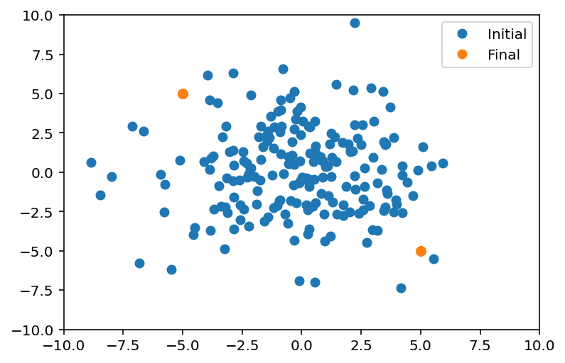
Figure 5: Experiments with four dimensional linear system (61)

with $p_{\text{target}}=\frac{1}{2}\delta_{x^{a}}+\frac{1}{2}\delta_{x^{b}}$ with $x^{a}=(-5,0,5,0)$ and $x^{b}=(5,0,-5,0)$. The initial and final distributions of the particles are shown.

V-4 Linear System

In this experiment, we consider the linear double integrator system with unstable damping with two position cooridinates and two velocity coordinates

$$\begin{aligned} \dot{x}_{1}&=x_{2},\ \ \dot{x}_{2}=x_{1}+u_{1}\ \ \dot{x}_{3}&=x_{2},\ \ \dot{x}_{4}=x_{3}+u_{2}\end{aligned}$$ (61)

The goal in this experiment is to stabilize the system to a sum of two Dirac measures $p_{\text{target}}=\frac{1}{2}\delta_{x^{a}}+\frac{1}{2}\delta_{x^{b}}$at $x_{a}=(-5,0,5,0)$ and $x^{b}=(5,0,-5,0)$. In this case, we use the controllability Grammian to compute the score function, and do not use any neural network. The distribution of the forward process $p^{f}_{t}$ is given in closed form as

$$p^{f}_{t}=K*p_{\text{target}}=\frac{1}{2}K(t,x^{a},y)+\frac{1}{2}K(t,x^{b},y)$$

where the function $K$ is defined in (54). The initial conditions are sampled from

$$p_{\infty}(x)=\frac{1}{(2\pi)^{d/2}{\rm det}(Q_{\infty})^{1/2}}e^{-\frac{1}{2}x^{T}Q^{-1}_{\infty}x}$$

where $Q_{\infty}$ is the infinite horizon controllability Grammian for the (open-loop stable) forward process with system $(A,B)$ matrices,

$$A=\begin{bmatrix}0&-1&0&0\\ 0&-1&0&0\\ 0&0&0&-1\\ 0&0&0&-1\\ \end{bmatrix},~~B=\begin{bmatrix}0&0\\ -1&0\\ 0&0\\ 0&-1\\ \end{bmatrix}.$$ (62)

Note that for the forward system, with system matrices are $(-A,-B)$. In Figure 5, we see that for this experiment the system is rendered bistable, and initial conditions are transported exactly to the target final states, depending on their initial conditions.

VI Conclusion

We presented an approach to control nonlinear systems inspired by denoising diffusion-based generative modeling. We established the existence of deterministic realizations of reverse processes that eliminate the need for stochasticity in feedback synthesis. Potential future directions include proving that the reverse process is asymptotically stabilizing under more general conditions. From a numerical standpoint, it may be beneficial to augment the score matching loss to explicitly promote stability, as the standard formulation does not guarantee that the learned control laws inherit the stabilizing properties of the ideal reverse dynamics.

Proof of Proposition IV.5.

The existence of and exponential stability of the solution of the NFE has been shown in [25, Theorem III.6]. The semigroup $\mathcal{T}(t)$ is known to be analytic [25, Theorem III.6] ,and hence, the solution satisfies $p\in D(\mathcal{A}^{a})$ for all $t\in(0,T]$. Therefore, the differentiability of the solution with respect to time follows from [43][Theorem 2.1.10]. ∎

References

- [1] Hassan K Khalil and Jessy W Grizzle. Nonlinear systems, volume 3. Prentice hall Upper Saddle River, NJ, 2002.
- [2] Francis Clarke. Functional analysis, calculus of variations and optimal control, volume 264. Springer, 2013.
- [3] Roger W Brockett et al. Asymptotic stability and feedback stabilization. Differential geometric control theory, 27(1):181–191, 1983.
- [4] Arthur J Krener. Feedback linearization. Mathematical control theory, pages 66–98, 1999.
- [5] Randy A Freeman and James A Primbs. Control lyapunov functions: New ideas from an old source. In Proceedings of 35th IEEE conference on decision and control, volume 4, pages 3926–3931. IEEE, 1996.
- [6] Lars Grüne, Jürgen Pannek, Lars Grüne, and Jürgen Pannek. Nonlinear model predictive control. Springer, 2017.
- [7] Derek Onken, Samy Wu Fung, Xingjian Li, and Lars Ruthotto. Ot-flow: Fast and accurate continuous normalizing flows via optimal transport. In Proceedings of the AAAI Conference on Artificial Intelligence, volume 35, pages 9223–9232, 2021.
- [8] Giovanni Bussi and Michele Parrinello. Accurate sampling using langevin dynamics. Physical Review E, 75(5):056707, 2007.
- [9] Ryan Turner, Jane Hung, Eric Frank, Yunus Saatchi, and Jason Yosinski. Metropolis-hastings generative adversarial networks. In International Conference on Machine Learning, pages 6345–6353. PMLR, 2019.
- [10] Jonathan Ho, Ajay Jain, and Pieter Abbeel. Denoising diffusion probabilistic models. Advances in neural information processing systems, 33:6840–6851, 2020.
- [11] Yang Song, Jascha Sohl-Dickstein, Diederik P Kingma, Abhishek Kumar, Stefano Ermon, and Ben Poole. Score-based generative modeling through stochastic differential equations. In International Conference on Learning Representations, 2020.
- [12] Gabriel Peyré, Marco Cuturi, et al. Computational optimal transport: With applications to data science. Foundations and Trends® in Machine Learning, 11(5-6):355–607, 2019.
- [13] Michael Janner, Yilun Du, Joshua Tenenbaum, and Sergey Levine. Planning with diffusion for flexible behavior synthesis. In International Conference on Machine Learning, pages 9902–9915. PMLR, 2022.
- [14] Cheng Chi, Siyuan Feng, Yilun Du, Zhenjia Xu, Eric Cousineau, Benjamin Burchfiel, and Shuran Song. Diffusion policy: Visuomotor policy learning via action diffusion. arXiv preprint arXiv:2303.04137, 2023.
- [15] Wenhao Li, Xiangfeng Wang, Bo Jin, and Hongyuan Zha. Hierarchical diffusion for offline decision making. In International Conference on Machine Learning, pages 20035–20064. PMLR, 2023.
- [16] Julen Urain, Niklas Funk, Jan Peters, and Georgia Chalvatzaki. Se (3)-diffusionfields: Learning smooth cost functions for joint grasp and motion optimization through diffusion. In 2023 IEEE International Conference on Robotics and Automation (ICRA), pages 5923–5930. IEEE, 2023.
- [17] Darshan Gadginmath and Fabio Pasqualetti. Dynamics-aware diffusion models for planning and control. arXiv preprint arXiv:2504.00236, 2025.
- [18] Andrei Agrachev and Paul Lee. Optimal transportation under nonholonomic constraints. Transactions of the American Mathematical Society, 361(11):6019–6047, 2009.
- [19] Alessio Figalli and Ludovic Rifford. Mass transportation on sub-riemannian manifolds. Geometric and functional analysis, 20:124–159, 2010.
- [20] Karthik Elamvazhuthi, Siting Liu, Wuchen Li, and Stanley Osher. Dynamical optimal transport of nonlinear control-affine systems. Journal of Computational Dynamics, 10(4):425–449, 2023.
- [21] Karthik Elamvazhuthi. Benamou-brenier formulation of optimal transport for nonlinear control systems on rd. arXiv preprint arXiv:2407.16088, 2024.
- [22] Kenneth F Caluya and Abhishek Halder. Finite horizon density steering for multi-input state feedback linearizable systems. In 2020 American Control Conference (ACC), pages 3577–3582. IEEE, 2020.
- [23] Efstathios Bakolas. Finite-horizon covariance control for discrete-time stochastic linear systems subject to input constraints. Automatica, 91:61–68, 2018.
- [24] Kazuhide Okamoto, Maxim Goldshtein, and Panagiotis Tsiotras. Optimal covariance control for stochastic systems under chance constraints. IEEE Control Systems Letters, 2(2):266–271, 2018.
- [25] Karthik Elamvazhuthi and Spring Berman. Density stabilization strategies for nonholonomic agents on compact manifolds. IEEE Transactions on Automatic Control, 69(3):1448 – 1463, 2024.
- [26] Gian Carlo Maffettone, Alain Boldini, Mario Di Bernardo, and Maurizio Porfiri. Continuification control of large-scale multiagent systems in a ring. IEEE Control Systems Letters, 7:841–846, 2022.
- [27] Diogo A Gomes and João Saúde. Mean field games models—a brief survey. Dynamic Games and Applications, 4:110–154, 2014.
- [28] Massimo Fornasier and Francesco Solombrino. Mean-field optimal control. ESAIM: Control, Optimisation and Calculus of Variations, 20(4):1123–1152, 2014.
- [29] Karthik Elamvazhuthi, Darshan Gadginmath, and Fabio Pasqualetti. Denoising diffusion-based control of nonlinear systems. IEEE 63rd Annual Conference on Decision and Control, 2024.
- [30] Jean-Claude Latombe. Robot motion planning, volume 124. Springer Science & Business Media, 2012.
- [31] Dominique Bakry, Ivan Gentil, Michel Ledoux, et al. Analysis and geometry of Markov diffusion operators, volume 103. Springer, 2014.
- [32] Filippo Santambrogio. Optimal transport for applied mathematicians. Birkäuser, NY, 55(58-63):94, 2015.
- [33] Brian DO Anderson. Reverse-time diffusion equation models. Stochastic Processes and their Applications, 12(3):313–326, 1982.
- [34] Ulrich G Haussmann and Etienne Pardoux. Time reversal of diffusions. The Annals of Probability, pages 1188–1205, 1986.
- [35] Patrick Cattiaux. Time reversal of diffusion processes with a boundary condition. Stochastic processes and their Applications, 28(2):275–292, 1988.
- [36] Andrei Agrachev, Davide Barilari, and Ugo Boscain. A comprehensive introduction to sub-Riemannian geometry, volume 181. Cambridge University Press, 2019.
- [37] Marco Bramanti et al. An invitation to hypoelliptic operators and Hörmander’s vector fields, volume 1298. Springer, 2014.
- [38] Roberto Monti and Daniele Morbidelli. Non-tangentially accessible domains for vector fields. Indiana University mathematics journal, pages 473–498, 2005.
- [39] Nicola Garofalo and Duy-Minh Nhieu. Lipschitz continuity, global smooth approximations and extension theorems for sobolev functions in carnot-carathéodory spaces. Journal d’Analyse Mathématique, 74(1):67–97, 1998.
- [40] Lawrence C Evans. Partial differential equations, volume 19. American Mathematical Society, 2022.
- [41] Luigi Ambrosio and Gianluca Crippa. Continuity equations and ode flows with non-smooth velocity. Proceedings of the Royal Society of Edinburgh Section A: Mathematics, 144(6):1191–1244, 2014.
- [42] El-Maati Ouhabaz. Analysis of heat equations on domains.(LMS-31). Princeton University Press, 2009.
- [43] Ruth F Curtain and Hans Zwart. An introduction to infinite-dimensional linear systems theory, volume 21. Springer Science & Business Media, 2012.