Offline Dynamic Inventory and Pricing Strategy: Addressing Censored and Dependent Demand

Abstract

In this paper, we study the offline sequential feature-based pricing and inventory control problem where the current demand depends on the past demand levels and any demand exceeding the available inventory is lost. Our goal is to leverage the offline dataset, consisting of past prices, ordering quantities, inventory levels, covariates, and censored sales levels, to estimate the optimal pricing and inventory control policy that maximizes long-term profit. While the underlying dynamic without censoring can be modeled by Markov decision process (MDP), the primary obstacle arises from the observed process where demand censoring is present, resulting in missing profit information, the failure of the Markov property, and a non-stationary optimal policy. To overcome these challenges, we first approximate the optimal policy by solving a high-order MDP characterized by the number of consecutive censoring instances, which ultimately boils down to solving a specialized Bellman equation tailored for this problem. Inspired by offline reinforcement learning and survival analysis, we propose two novel data-driven algorithms to solving these Bellman equations and, thus, estimate the optimal policy. Furthermore, we establish finite sample regret bounds to validate the effectiveness of these algorithms. Finally, we conduct numerical experiments to demonstrate the efficacy of our algorithms in estimating the optimal policy. To the best of our knowledge, this is the first data-driven approach to learning optimal pricing and inventory control policies in a sequential decision-making environment characterized by censored and dependent demand. The implementations of the proposed algorithms are available at https://github.com/gundemkorel/Inventory_Pricing_Control

1 Introduction

In today’s data-rich business environment, the vast availability of historical data, especially in retail and tech sectors, has sparked significant interest in implementing feature-based pricing and ordering strategies within the framework of sequential decision-making. If firms, especially in the retail and tech sectors, can utilize this data effectively alongside machine learning and optimization tools, they can make near-optimal, sequential pricing and ordering decisions to meet anticipated demand, maximize profit, and minimize missed revenue opportunities due to stockouts in the long run.

Navigating this process necessitates that the historical data includes the true demand information. However, the primary challenge with a typical historical data is its inherent limitation in reflecting the true demand due to censoring. In other words, when the demand surpasses available inventory, stockouts occur, leading customers to leave without making a purchase. As a result, the recorded sales reflect only the minimum of the true demand and available inventory at hand, implying that the historical data does not contain the actual demand information when the censoring is present. This skew in the data can lead to biased profit estimates if the sales data is mistakenly treated as the true demand. The issue becomes more convoluted by the fact that the demand often exhibits past-dependent characteristics, especially in retail, where yesterday’s demand influences today’s. Therefore, any method that seeks to use the historical data to optimize pricing and ordering decisions must account for the demand censoring along with the past-dependent nature of the demand in its approach.

1.1 A Problem Statement, Challenges, and A Motivating Application

In this paper, we tackle the data-driven sequential decision-making problem under the dependent and censored demand within an offline framework. In particular, we focus on a scenario where a firm lacks the knowledge of the true demand function, which exhibits past-dependent characteristics, but has access to an offline dataset containing historical prices, ordering quantities, inventory levels, covariates, and sales data. The firm’s objective is to use this offline data to develop an optimal feature-based joint pricing and inventory policy that maximizes the expected total profit in the long run.

The biggest challenge in this context is the censor of the demand. When the demand exceeds the available inventory, it becomes unobservable. This issue is further compounded by the history-dependent nature of demand and the offline learning paradigm where there is no interaction with the environment. While previous research in online learning setting has explored pricing and/or inventory control models that account for dependent and/or censored demand (e.g., Chen & Song, 2001; Lu et al., 2005, 2008; Keskin et al., 2022; Chen et al., 2020, 2024), the simultaneous integration of these demand characteristics into offline pricing and inventory control models remains largely unexplored (e.g., Levi et al., 2007; Qin et al., 2022).

Furthermore, the interactions between pricing, inventory levels, and the demand necessitate simultaneous optimization for profitability. For instance, if prices are set too high, the demand may drop, leading to excess inventory and higher holding costs. Conversely, if prices are set too low but not enough ordering is placed, the demand surges, potentially resulting in censoring, stock-outs, and thus, missed sales opportunities. Therefore, a well-structured and data driven approach that jointly addresses sequential pricing and inventory control along with the dependent and censored demand is essential for achieving maximum profitability.

The practical relevance of our methodology is evident in the retail industry, particularly for companies like CVS. For instance, during the COVID-19 pandemic, the demand for products like face masks or sanitizers surged dramatically, leading to successive stockouts, and thus, consecutive demand censoring. Companies had to navigate these challenges carefully to ensure an adequate supply while avoiding overstocking once demand stabilized. By leveraging extensive data on the purchasing patterns, companies could develop strategies that effectively align pricing with inventory management, ensuring both profitability and the availability of essential products, such as masks and sanitizers, even during the black-swan events like COVID-19. Consequently, it is critical for firms to have a robust, data-driven sequential pricing and inventory control strategy that accounts for the complexities of the censored and history-dependent demand. When implemented correctly, it does not only make firms better positioned to handle future market conditions, which results in achieving sustained profitability and operational efficiency, but also addresses broader societal challenges, such as meeting public health needs, as demonstrated in this example.

1.2 Main Results and Contributions

Because the demand censoring can obscure true demand, existing offline policy learning methods that neglect this issue and treat sales quantity as the realized demand can lead to misinformed strategies that do not align well with actual market conditions and the goal of companies. Moreover, even methods that acknowledge censoring but operate under the assumption of the independent demand across periods can produce flawed outcomes as the demand generally exhibits dependent characteristics in reality. This failure can further complicate the development of reliable pricing and inventory control policies, potentially leading to decisions that are not only sub-optimal but also detrimental to the long-term business performance.

Motivated by these, we develop two novel data-driven offline learning algorithms that factor in the dependent and censored demand. By leveraging the offline data, the proposed algorithms provide a near-optimal feature-based pricing and inventory control strategy in a sequential manner as the sample size increases. To the best of our knowledge, we are the first to tackle the problem of sequential feature-based pricing and inventory control when the demand is censored and dependent.

Our approach starts by modeling the environment as an infinite-horizon time-homogeneous Markov Decision Process (MDP), assuming that the demand is observable without any censoring. This serves as a benchmark to understand how the censoring affects the process. Unlike the most existing methods that assume the demand is independent and identically distributed (i.i.d.) across periods, we consider the first-order dependence by incorporating the demand into the state space dynamics to better capture the complexity of the real-world. Then since demand is censored in reality, we concentrate on the observed process, where censoring is allowed, to model how offline data is actually generated. In particular, this observed process not only accounts for the demand censoring but also the potential failure of the Markov property as a result of censoring. In summary, our framework extends previous works (e.g., Harsha et al., 2021; Qin et al., 2022; Liu & Zhang, 2023) by relaxing the assumptions of i.i.d. demand and no censoring.

Under our general modeling framework, a significant challenge arises in finding an optimal pricing and inventory control policy due to the demand censoring. Specifically, the censor of the demand results in partial observability of both current and future states, which obscures the true structure of the optimal policy, and potentially, renders it non-stationary. This contrasts with classical time-homogeneous MDP settings, where an optimal stationary policy always exists. Learning an optimal non-stationary policy for an infinite-horizon process poses significant challenges, particularly when relying solely on the finite-horizon offline data. Additionally, the standard Bellman equation, essential for many RL algorithms, does not apply to non-stationary policies and fails under the breakdown of the Markov property, further complicating the development of a valid offline algorithm. To address these challenges, we demonstrate that finding an optimal policy under the observed process is almost equivalent to identifying an optimal policy for a specific high-order MDP, which is characterized by multiple optimal Q-functions based on the maximum number of consecutive censoring instances. Leveraging this insight, we introduce two novel algorithms: Censored Fitted Q-Iteration (C-FQI) and Pessimistic Censored Fitted Q-Iteration (PC-FQI). These algorithms are designed to learn the multiple optimal Q-functions, and accordingly, derive the estimated policies from the offline data. Our approaches are inspired by the well-known FQI algorithm and the principle of pessimism (e.g., Ernst, Geurts, Wehenkel & Littman, 2005; Buckman et al., 2020; Jin et al., 2021).

Theoretically, we provide a finite-sample regret analysis for our offline learning algorithms under general conditions. We demonstrate that these algorithms can asymptotically recover the optimal policy under three key conditions stated below.

The first key condition pertains to censoring, where we introduce a new concept unique to our problem setting and termed as censoring coverage. This concept complements the well-established notion of state-action coverage in offline policy learning (Levine et al., 2020; Foster et al., 2021; Fujimoto et al., 2019; Wang et al., 2020). Censoring coverage assesses the potential discrepancy between the maximum number of consecutive censoring instances that could occur under the optimal policy and the offline data distribution. This allows us to capture the complexities that the demand censoring induces into our modeling framework. Specifically, if the offline data exhibits fewer consecutive censoring instances than those that could be observed under the optimal policy, it indicates a lack of coverage of all possible trajectories that the optimal policy might produce—referred to as insufficient censoring coverage. To illustrate the obstacle brought by insufficient censoring coverage, consider the example of luxury watches and high-end bags in the retail sector. An optimal policy might deliberately order fewer items than the anticipated demand to create an aura of exclusivity and scarcity, which can result in a high number of consecutive demand censoring but significantly higher prices, and thus, profits in the future. The offline data from typical sales operations, on the other hand, may show fewer such instances. This discrepancy makes it infeasible to fully learn the optimal policy from the offline data, as it does not accurately represent all the scenarios that would occur under the optimal policy. Therefore, ensuring the sufficient censoring coverage is crucial for accurately recovering the optimal policy using the offline data. Secondly, during iterations of the proposed algorithms, the estimated policy is designed to select an action that maximizes the estimated long-term value. When the estimated policy encounters the maximum number of consecutive censoring instances that could occur under the optimal policy, choosing an action that results in further censoring leads to inconsistencies and impede the recovery of the optimal policy. Therefore, it is crucial that the action chosen by the estimated policy in this specific case avoids causing additional censoring, making this the second essential condition for accurately learning the optimal policy. Thirdly, we require the final estimated policy, when deployed in the real world, to select an action that avoids another censored state in the case of facing with the maximum number of consecutive censoring instances observed in the offline data. This requirement is crucial because if the estimated policy encounters more consecutive censoring instances than those present in the offline data, it might lack the necessary information to act. However, the challenge arises when the action chosen to avoid further censoring does not maximize the long-term value. Therefore, ensuring that this action is an optimal one is another key condition for recovering the optimal policy.

Furthermore, to empirically test our algorithms, we conduct simulation studies across various settings. The results from these simulations further support our theoretical analysis, confirming the effectiveness of our algorithms in optimizing pricing and inventory control strategies.

Finally, it is noteworthy and of independent interest that this work presents the first regret analysis of the FQI algorithm without requiring the full coverage assumption. Additionally, we provide a direct comparison of the regrets between FQI and Pessimistic FQI—a comparison previously considered infeasible in the literature due to different assumptions. Our analysis reveals that both algorithms share the same convergence rate under the same conditions.

1.3 Literature Review

Our work is related to the following streams of literature.

Offline Data-Driven Algorithms for Pricing and Inventory Control. Offline learning, where the entire dataset is pre-collected before the algorithm is deployed, proves particularly valuable in scenarios where online exploration is either too costly or impractical. Furthermore, it can lay the foundation for a warm start in online learning. Despite the extensive research in offline data-driven inventory management, tackling joint pricing and inventory control in a sequential context, especially under the dependent and censored demand, remains uncharted in the literature. Most offline learning algorithms tend to focus exclusively on either pricing or inventory control, often within a single-period framework, and neglect the complexities caused by the demand censoring. In contrast, our work tackles pricing and inventory control jointly in a sequential manner and fully accounts for the effects of the censored and dependent demand.

Specifically, prior studies in inventory management, such as Levi et al. (2007) and Cheung & Simchi-Levi (2019), introduced algorithms for multi-period inventory control using offline data. These methods utilize the Sample Average Approximation (SAA) to solve ordering decisions based on forecasted demand. However, as noted by Feng & Shanthikumar (2022), SAA is prone to overfitting and is unsuitable for our problem because there is another decision variable (price) which influences the demand distribution. On top of these works focusing solely on inventory control, they further assumed no demand censoring and did not consider the feature information, limiting their applicability. In contrast, Ban & Rudin (2019) applied machine learning to a data-driven newsvendor model with the feature information, but their study is restricted to a single period and neglected both pricing decisions and demand censoring. Similarly, Lin et al. (2022) focued on the traditional newsvendor problem with a risk constraint on the profit and contextual information. However, their work fundamentally differs from ours, as they did not account for how the decision (price in our problem) affects uncertainty (demand). Overall, in traditional newsvendor problems, supply decisions do not influence demand (i.e. no decision-dependent uncertainty), making those problems special cases of the problem we aim to solve.

In pricing optimization, Qi et al. (2022) and Bu et al. (2023) examined pricing problems with the censored demand in an offline setting. These works are limited to single-period scenarios and do not consider inventory management. Furthermore, Wang & Liu (2023) and Miao et al. (2023) utilized the causal inference framework to explore feature-based pricing problems under approximate or invalid instrumental variables. However, their approaches, which do not account for the censored demand along with inventory decisions, and again, are limited to single-period settings, are fundamentally distinct from ours. In contrast, our approach bridges these gaps by incorporating relevant feature information, considering pricing and inventory management jointly, and operating under a multi-period setting along with the censored and dependent demand.

More closely related to our work, Qin et al. (2019) proposed a data-driven approximation algorithm for joint pricing and inventory control in a multi-period setting using the offline data. However, they assumed that demand is fully observable (i.e. no censoring). Additionally, they did not take into account any feature information. On the contrary, our work allows demand censoring and incorporate feature information, implying that their work is a special case of ours. Furthermore, Harsha et al. (2021) developed a procedure for solving the price-setting newsvendor problem. However, their work is limited to the single period setting and does not take into account the censor of the demand, which, overall, render our framework as generalization of theirs. In a similar fashion, Liu & Zhang (2023) investigated a data-driven pricing newsvendor problem, aiming to maximize profit by setting inventory and pricing levels based on the historical demand and feature data. They assumed fully observable historical demand and focus on a single-period optimization. By comparison, our approach accounts for the demand censoring and operates in a multi-period setting.

Overall, our work differs from the previous works by tackling the pricing and inventory control jointly under censored and dependent demand in a multi-period setting. Our approach not only introduces a new dimension to the existing literature but also generalizes current problem settings, making them special cases of our work, such as focusing exclusively on inventory control or relaxing the demand censoring constraint.

Policy Learning through Offline Reinforcement Learning. The field of offline policy learning within the reinforcement learning (RL) framework has garnered significant attention in both computer science and statistics. Traditional offline RL approaches are typically built on the framework of MDPs (Bertsekas, 1995; Sutton & Barto, 2018). Under this framework, it is well known that an optimal policy can be derived based on the optimal Q-function, obtained through solving the Bellman equation which relies on the Markov property (e.g., Ernst, Geurts & Wehenkel, 2005; Riedmiller, 2005; Jin et al., 2021; Kumar et al., 2020). However, in our problem setting, existing offline RL methods fall short due to two primary challenges: the failure of the Markov property caused by the censored demand and the absence of reward information at censored data points.

Firstly, the failure of the Markov property as a result of the censored demand prevents us from characterizing the optimal policy using the standard Q-function, the cornerstone of conventional offline RL algorithms. In classical MDP settings, an optimal stationary policy always exists and it takes the greedy action with respect to the optimal Q-function. But, in our case, the structure of the optimal policy becomes unknown, potentially non-stationary and non-Markovian. We demonstrate that identifying the optimal policy is nearly equivalent to solving for an optimal policy within a specific high-order MDP, characterized by multiple optimal Q-functions that depend on consecutive censoring instances and can be obtained through an alternative form of Bellman equation tailored for our problem setting.

Secondly, the most existing offline RL algorithms assume that the offline data contains complete reward information throughout the observation period. In our scenario, however, reward information is missing at censored data points, which complicates the direct application of standard methods. To overcome this, we employ advanced survival analysis techniques to impute the missing reward information by generalizing the idea proposed in Qi et al. (2022).

With the alternative form of Bellman equation catered for our problem setting and imputed rewards, we adapt the idea of FQI algorithm to our specific context, leading to the development of the Censored Fitted Q-Iteration (C-FQI) algorithm. This algorithm is designed to approximate the aforementioned Bellman equation from the offline data with imputed reward information, and accordingly, output a near-optimal and data-driven policy.

Furthermore, a typical challenge in offline reinforcement learning is insufficient data coverage, which stems from the static nature of historical data and the lack of exploration. This issue arises in our problem as well and often leads to distribution shift, where the optimal policy differs significantly from the data available for training (Wang et al., 2020; Levine et al., 2020). Recent research has aimed to address this challenge by adopting a pessimistic approach in policy optimization, minimizing exploration of rarely encountered state-action pairs within the batch data. This approach has been shown to mitigate the risks associated with insufficient data coverage and has led to the development of new algorithms based on pessimism principle (Kumar et al., 2020; Fujimoto et al., 2019; Liu et al., 2020; Rashidinejad et al., 2021; Jin et al., 2021; Zanette et al., 2021; Zhan et al., 2022; Fu et al., 2022). In our work, we incorporate the pessimism principle into the C-FQI algorithm to address extrapolation error and possibly enhance its performance in pricing and inventory control tasks, leading to the development of PC-FQI. This approach allows us to extend the applicability of our method to real-world scenarios where the offline data coverage is often limited.

1.4 Structure

The remainder of this paper is organized as follows: In Section 2, we introduce the preliminary model, notations, and challenges in data-driven sequential pricing and inventory control with the censored and dependent demand. In Section 3, we elaborate on the proposed solutions, including the implementation of the data-driven offline learning algorithms C-FQI and PC-FQI. In Section 4, we present the theoretical analysis of these algorithms, including their finite-sample regret guarantees. In Section 5, we provide the results on numerical studies used to evaluate the effectiveness of our proposed algorithms. In Section 6, we conclude the paper with key insights and suggestions for future research. Finally, the proofs of all the lemmas and theorems along with the details of numerical results are given in Appendix.

2 Problem Formulation

2.1 Preliminaries and Notations

Consider a single trajectory ${(S_{t},A_{t},R_{t})}_{t\geq 0}$ of states, actions, and rewards in an inventory and pricing decision process. At each decision point $t$, the state $S_{t}=(X_{t},Y_{t},D_{t-1})$ is observed, where the state space is given by ${\cal S}=\mathscr{X}\otimes\mathscr{Y}\otimes\mathscr{D}$. Specifically, $X_{t}$ represents $p$-dimensional features with the space $\mathscr{X}\subseteq\mathbb{R}^{p}$, $Y_{t}$ denotes non-negative inventory levels with the space $\mathscr{Y}\subseteq\mathbb{R}^{+}$, and $D_{t-1}$ is the total demand over the time interval $[t-1,t)$, with the space $\mathscr{D}\subseteq\mathbb{R}^{+}$. The action variable $A_{t}=(P_{t},O_{t})$ includes price ($P_{t}\in\mathscr{P}\subseteq\mathbb{R}^{+}$) and ordering quantity ($O_{t}\in\mathscr{N}\subseteq\mathbb{R}^{+}$), with the action space ${\cal A}={\cal P}\otimes{\cal N}$. The reward $R_{t}$ is given by:

$$R_{t}=\underbrace{P_{t}\min(Y_{t},D_{t})}_{\begin{subarray}{c}\text{Sales}\\ \text{Revenue}\end{subarray}}-\underbrace{C_{1,t}(D_{t}-Y_{t})}_{\begin{subarray}{c}\text{Stock-out }\\ \text{Cost}\end{subarray}}\mathbb{I}(\Delta_{t}=0)-\underbrace{C_{2,t}O_{t}}_{\begin{subarray}{c}\text{Ordering}\\ \text{Cost}\end{subarray}}-\underbrace{C_{3,t}(Y_{t}-D_{t})}_{\begin{subarray}{c}\text{Inventory}\\ \text{Cost}\end{subarray}}\mathbb{I}(\Delta_{t}=1),$$ (1)

where $C_{1,t}$, $C_{2,t}$, and $C_{3,t}$ are per unit stock-out, ordering, and inventory costs at time $t$, respectively. Without loss of generality, we assume $C_{i,t}$ are known and deterministic numbers. In general, one can allow $C_{i,t}$, for $i=1,2,3$, to change dynamically over time and thus they can be incorporated into the state space. For simplicity, throughout this paper, we assume $R_{t}$ is uniformly bounded by $R_{\max}$, i.e., $|R_{t}|\leq R_{\max}$. Finally, it is important to note that $D_{t-1}$ is included in the state variables at time $t$ because it is realized only after the pricing and ordering decisions are made at time $t-1$ (i.e. $D_{t-1}$ naturally depends on $P_{t-1}$).

Figure 1: Transition dynamics of the underlying decision process ${\{S_{t},A_{t},R_{t}\}}_{t\geq 0}$; Given the current state $S_{t}$ and action $A_{t}$, the transition to the next state $S_{t+1}$ and reward $R_{t}$ is independent of all prior states and actions.

The decision process ${(S_{t},A_{t},R_{t})}_{t\geq 0}$ is characterized by a policy $\pi=\{\pi_{1},\pi_{2}\}$, where $\pi_{1}$ and $\pi_{2}$ are the pricing and inventory replenishment strategies, respectively. Such a policy $\pi$ might be history-dependent (i.e. $\pi$=$\{\pi_{t}\}_{t\geq 0}$=$\{\pi_{1}=\{\pi_{1,t}\}_{t\geq 0},\pi_{2}=\{\pi_{2,t}\}_{t\geq 0}\}$ where $\pi_{t}=\{\pi_{1,t},\pi_{2,t}\}:H^{{}^{\prime}}_{t,\text{MDP}}=\left\{S_{j},A_{j}\right\}_{0\leq j\leq t}\setminus A_{t}\rightarrow\Delta({\cal A}),\forall t\geq 0$), or stationary if there exists a function $\widetilde{\pi}=(\widetilde{\pi}_{1},\widetilde{\pi}_{2})$ such that $\pi_{t}(\bullet|H^{{}^{\prime}}_{t,\text{MDP}})=\{\widetilde{\pi}_{1}(\bullet|S_{t}),\widetilde{\pi}_{2}(\bullet|S_{t})\}$ almost surely for any $t\geq$ 0.

We propose to use a first order time-homogeneous MDP to model $\{(S_{t},A_{t},R_{t})\}_{t\geq 0}$ with the following assumptions:

$$(S_{t+1},R_{t})\,|\,S_{t},A_{t}\mathchoice{\mathrel{\hbox to0.0pt{$\displaystyle\perp$\hss}\mkern 2.0mu{\displaystyle\perp}}}{\mathrel{\hbox to0.0pt{$\textstyle\perp$\hss}\mkern 2.0mu{\textstyle\perp}}}{\mathrel{\hbox to0.0pt{$\scriptstyle\perp$\hss}\mkern 2.0mu{\scriptstyle\perp}}}{\mathrel{\hbox to0.0pt{$\scriptscriptstyle\perp$\hss}\mkern 2.0mu{\scriptscriptstyle\perp}}}H_{t-1,\text{MDP}},\text{ and the transition is time-homogenous},$$ (2)

where $H_{t-1,\text{MDP}}=\left\{S_{t},A_{t}\right\}_{0\leq t\leq t-1}$. The diagram in Figure 1 shows the dynamics of this decision process.

It is worth nothing that this modeling framework, on top of being non-parametric, incorporates first-order dependency of the demand into the state-space dynamics and can be extended to higher-order Markov decision processes to capture any existing higher-order dependencies. This generalizes existing models in the joint pricing and inventory control literature, which often implicitly assume that the demand is independent across periods once the past prices are controlled (e.g., Petruzzi & Dada, 2002; Araman & Caldentey, 2009; Feng et al., 2014; Chen et al., 2017). By including additional factors that affect demand, such as the state of the economy incorporated into $X_{t}$, our framework allows demand to be dependent across periods even when the prices are controlled. If all external features are excluded, our model reduces to the conventional case where demand is independent across periods given prices. Furthermore, our framework accommodates reference price effects observed in consumer behavior (e.g., Chen et al., 2020). For example, consider a demand function $D_{t}=b-ap_{t}+c(r_{t}-p_{t})$, where the reference price $r_{t}$ evolves according to $r_{t}=\alpha r_{t-1}+(1-\alpha)p_{t-1}$. Here, $r_{t}$ becomes part of the action $A_{t}$, allowing the model to incorporate past prices and capture the impact of consumers’ price expectations on current demand.

Under this framework, it is well-established that a stationary and optimal pricing and inventory replenishment policy exists, i.e., $\pi_{\text{oracle}}^{*}=(\pi_{1,\text{oracle}}^{\ast},\pi_{2,\text{oracle}}^{\ast})$, that maximizes the expected discounted cumulative rewards,

$$\pi_{\text{oracle}}^{*}\in\text{argmax}_{\pi}\,\mathbb{E}_{\textbf{MDP}}^{\pi}[\sum_{t=0}^{\infty}\gamma^{t}R_{t}],$$ (3)

where $\mathbb{E}_{\textbf{MDP}}^{\pi}$ means all actions along the trajectory follows $\pi$, the subscript ”MDP” is used to differentiate the expectation operator of the underlying MDP from that of the observed process with demand censoring incorporated defined in the following section and $\gamma\in[0,1)$ is a discount factor.

One popular solution to obtain $\pi_{\text{oracle}}^{*}$ is to find an optimal Q-function and take point-wise maximum with respect to action for every state. Specifically,

$$\pi_{\text{oracle}}^{*}(a\,|\,s)=\begin{cases}1&\text{if}\;a=\text{argmax}_{a^{\prime}\in{\cal A}}Q^{*}(s,a^{\prime})\\ 0&\text{otherwise},\end{cases}$$ (4)

where $Q^{*}(s,a)=\sup_{\pi}\mathbb{E}_{\textbf{MDP}}^{\pi}\left[\sum_{t=0}^{\infty}\gamma^{t}R_{t}\,|\,(S_{0},A_{0})=(s,a)\right]$ for every $s\in{\cal S}$ and $a\in{\cal A}$. When defining $\pi_{\text{oracle}}^{*}$, without loss of generality, we assume the uniqueness of the maximum with respect to $Q^{\ast}$. In an offline setting, assuming full demand information is available, $Q^{\ast}$ can be estimated through classical algorithms such as FQI (Ernst, Geurts & Wehenkel, 2005), and thus, enabling the derivation of near-optimal and data-driven policies.

2.2 Our Problems and Challenges

Unfortunately, the real-world offline data, particularly in retail, often lacks the complete demand information due to censoring. Typically, only the sales quantity, denoted by $Z_{t}=\min(Y_{t},D_{t})$ with the space $\mathscr{Z}$, is observed. In other words, the offline data is realized through what we term as the observed process $\{W_{t},A_{t},R_{t}\mathbb{I}[\Delta_{t}=1]\}_{t\geq 0}$, where $W_{t}=(X_{t},Y_{t},Z_{{t-1}},\Delta_{t-1})$ with space $\mathscr{W}$, instead of $\{S_{t},A_{t},R_{t}\}_{t\geq 0}$. Clearly, in the observed process, the reward information is also missing when the demand is censored. Furthermore, the Markov property from Equation (2) is violated under offline data distribution when censoring occurs (i.e., $Z_{t-1}\neq D_{t-1}$). Consequently, offline data with incomplete demand information is not sufficient for learning $\pi^{\ast}_{\text{oracle}}$. The observed process is illustrated in Figure 2.

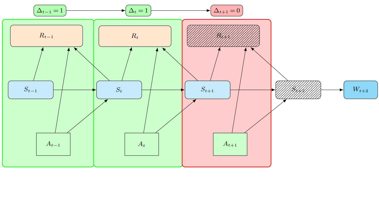
Figure 2: Depiction of a trajectory under the observed process $\{W_{t},A_{t},R_{t}\mathbb{I}[\Delta_{t}=1]\}_{t\geq 0}$, where $\Delta_{t}$ is the censoring indicator. When $\Delta_{t}=1$ (no censoring), the reward, $R_{t}$, and the demand, $D_{t}$, are observable, rendering $S_{t+1}=W_{t+1}\setminus\Delta_{t}=1$. However, when censoring occurs while moving from time step $t+1$ to $t+2$ (i.e $\Delta_{t+1}=0$) , the reward $R_{t+1}$ and demand $D_{t+1}$ become unobservable, and thus, the state $S_{t+2}$. This implies that $S_{t+2}\neq W_{t+2}\setminus\Delta_{t+1}=0$. The shaded boxes represent these censored elements, highlighting the transition to limited observability under censoring, where $W_{t+2}$ does not contain as much information as $S_{t+2}$. This figure emphasizes the impact of censoring on the process dynamics.

Under these constraints, we instead aim to find the optimal policy defined under the observed process, i.e.,

$$\pi^{*}\in\text{argmax}_{\pi\in\Pi}\mathbb{E}^{\pi}[\sum_{t=0}^{\infty}\gamma^{t}R_{t}\,|\,W_{0}],$$ (5)

where the expectation is taken over the trajectories generated by $\pi$ under the observed process $\{W_{t},A_{t},R_{t}\mathbb{I}[\Delta_{t}=1]\}_{t\geq 0}$, with $\Pi$ representing the set of all policies associated with this process. Here, $W_{0}$ follows $\nu(\bullet)$ which is some reference distribution over the initial observation and is predetermined and known by decision makers. This is a typical assumption in the literature of RL. In the following, we demonstrate how offline data can be used to find $\pi^{\ast}$, with an additional assumption on our data-generating process.

Assumption 1.

The offline data $\mathscr{O}_{N}=\{W_{i,t},A_{i,t},W_{i,t+1},R_{i,t}\mathbb{I}[\Delta_{i,t}=1]\}^{1\leq i\leq N}_{0\leq t<T-1}$ is generated by the policy, $\pi^{b}\in\Pi$, where each trajectory is an i.i.d. copy from $\{W_{t},A_{t},R_{t}\mathbb{I}[\Delta_{t}=1]\}_{t\geq 0}$.

In RL literature, $\pi^{b}$ is often referred to as the behavior policy. The behavior policy may not be known beforehand and can be history-dependent. Using $\mathscr{O}_{N}$, we aim to develop an algorithm that returns an estimated policy $\widehat{\pi}$ with diminishing regret when the sample size $N$ (and/or $T$) is large, where the regret of $\widehat{\pi}$ is defined as:

$$\textbf{Regret}(\widehat{\pi})\triangleq\mathbb{E}^{\pi^{*}}[\sum_{t=0}^{\infty}\gamma^{t}R_{t}]-\mathbb{E}^{\widehat{\pi}}[\sum_{t=0}^{\infty}\gamma^{t}R_{t}].$$ (6)

To achieve this goal, several challenges must be addressed. Before elaborating on these challenges, we introduce a crucial concept that helps us characterize the structure of the observed process:

Definition 1.

Let $n_{T^{\prime},b}$ and $n_{T^{\prime},\ast}$ represent the maximum number of consecutive censoring instances observed across all possible trajectories generated by $\pi^{b}$ and $\pi^{\ast}$, respectively, within a window of length $T^{\prime}$.

More rigorous definition can be found in Definition 10 of the Appendix. The first challenge stems from the nature of the offline data. Let $\hat{n}_{T^{\prime},b}$ denote the sample estimation of ${n}_{T^{\prime},b}$. When the estimated (or learned) policy is deployed in the real world, it might encounter more consecutive censoring instances than $\hat{n}_{T,b}$. In these scenarios, the learned policy is ill-prepared to respond effectively, as it has not encountered such cases during training, as shown in Figure 3. Consequently, it is essential that the learned policy avoids generating more consecutive censoring instances than those observed in the offline data when deployed in the real world.

Figure 3: Simplified illustration of offline data with respect to consecutive censoring. The x-axis represents the number of consecutive censoring instances, while the y-axis (A) shows the action space. Green dots represent observed state-action pairs in the offline data. For example, there are two observations with 4 consecutive censoring instances where actions $a_{2}$ and $a_{4}$ were taken. The vertical dashed blue line indicates the maximum consecutive censoring in the offline data. The red shaded area with a question mark represents the region where the learned policy lacks training data, potentially leading to suboptimal decisions when deployed in the real world if encountered.

Secondly, the true structure of the optimal policy, $\pi^{\ast}$, under the observed process is unknown due to the effects of the demand censoring, which subsequently leads to the failure of the Markov property. In addition, this failure potentially makes the optimal policy non-stationary, which contradicts with the classical MDP. Learning a non-stationary policy for an infinite-horizon decision process presents a significant challenge, especially when we can only observe a finite-horizon process. Furthermore, the standard Bellman equation, which depends on the Markov property and underpins many RL algorithms, becomes inapplicable under non-stationary policies, leading to the curse of horizon. This significantly hampers our ability to develop an effective offline algorithm.

Thirdly, the coverage of the offline data with respect to $\pi^{\ast}$ is crucial for accurately approximating it. In our problem, coverage has two key layers. The first, which applies to all offline problems, is the state-action coverage, which measures how well the offline data represents the state-action distribution induced by the optimal policy. This issue has been widely studied in literature (e.g., Uehara & Sun, 2021; Jin et al., 2021; Rashidinejad et al., 2021; Yin & Wang, 2021; Lu et al., 2022; Rashidinejad et al., 2022). The second, unique to our problem, is the censoring coverage. This measures potential discrepancy between the maximum number of consecutive censoring instances occurred under the distributions induced by both the optimal and behavior policies (i.e., $n_{T^{\prime},\ast}$ and $n_{T^{\prime},b}$). In particular, if $n_{T^{\prime},\ast}>n_{T^{\prime},b}$, the offline data lacks sufficient censoring coverage to accurately learn the optimal policy which is illustrated by Figure 4. Finally, this issue is exacerbated by the fact that $n_{T^{\prime},\ast}$ and $n_{T^{\prime},b}$ are unknown quantities, though $n_{T^{\prime},b}$ can be estimated.

(a)

(b)

Figure 4: Illustrations of Censoring Coverage between Optimal and Behavior Policies. (a) Sufficient censoring coverage scenario: the behavior policy (blue) has sufficient censoring coverage over the optimal policy (red), and thus, all the trajectories under the optimal policy can be learnt from the offline data as indicated by green shaded area. (b) Insufficient censoring coverage scenario: the behavior policy does not have sufficient censoring coverage over the the optimal policy, and thus, the trajectories under the optimal policy with more than $n_{T^{\prime},b}$ consecutive censoring can not be learnt from the offline data as illustrated by red shaded area. The x-axis represents the window size, while the y-axis shows the number of consecutive censoring instances. $n_{T^{\prime},b}$ and $n_{T^{\prime},*}$ represent the maximum number of consecutive censoring instances for the behavior and optimal policies within the window size of $T^{\prime}$, respectively.

Lastly, when the demand is censored, the reward is also censored because of the stock-out cost in Equation (1). This lack of information further complicates the development of an effective data-driven algorithm for learning $\pi^{\ast}$.

In the following, we present our approaches that tackles these aforementioned challenges and eventually find $\widehat{\pi}$ that is close to $\pi^{\ast}$ in terms of the regret.

3 Our Proposal

3.1 Overview

For the remainder of this paper we assume, without loss of generality, that there is no censoring at the beginning of the observed process, meaning $D_{-1}$ is known or $\Delta_{-1}=1$. Furthermore, before giving an overview on our proposed methods to address the aforementioned challenges, we first introduce an event related to consecutive censoring.

Definition 2.

$\mathscr{C}(T^{\prime},n)=\left\{\mathscr{O}=\{W_{t},A_{t},R_{t}\mathbb{I}[\Delta_{t}=1]\}_{t\geq 0}\,\mid\,C_{T^{\prime}}(\mathscr{O})\leq n\right\}$, where $C_{T^{\prime}}(\mathscr{O})$ denotes the maximum number of consecutive censoring up to time step $T^{\prime}$ under the observed process.

To address the first challenge, we require the final learned policy not to generate more consecutive censoring instances than what is observed in the first $K$ horizon of the offline data by leveraging Assumption 2, where $K$ is the number of iterations in our proposed algorithms, to be specified later. This ensures that our learned policy can be deployed in every scenario in the testing environment. If this condition is met, the following regret decomposition holds; otherwise, it does not.

$$\textbf{Regret}(\widehat{\pi}) =(\underbrace{\mathbb{E}^{\pi^{*}}[\sum_{t=0}^{\infty}\gamma^{t}R_{t}\,|\,\mathscr{C}(K,n_{K,b})]-\mathbb{E}^{\widehat{\pi}}[\sum_{t=0}^{\infty}\gamma^{t}R_{t}]}_{(i)})\operatorname{Pr}^{\pi^{*}}(\mathscr{C}(K,n_{K,b}))$$

$$+\underbrace{(\mathbb{E}^{\pi^{*}}[\sum_{t=0}^{\infty}\gamma^{t}R_{t}\,|\,\mathscr{C}^{c}(K,n_{K,b})]-\mathbb{E}^{\widehat{\pi}}[\sum_{t=0}^{\infty}\gamma^{t}R_{t}])\operatorname{Pr}^{\pi^{*}}(\mathscr{C}^{c}(K,n_{K,b}))}_{(ii)},$$ (7)

where, for the sake of simplicity, we assume $\hat{n}_{K,b}=n_{K,b}$ which will be relaxed in our theoretical analysis. Based on Equation (3.1), ideally one should find a learned policy $\widehat{\pi}$ such that both the term $(i)$ and $(ii)$ are minimized simultaneously. However, this regret decomposition reveals an important role of the censoring coverage related to Definition 1. On the one hand, term $(i)$ represents the portion of $\pi^{*}$ that can be learned, thanks to sufficient censoring coverage within the first $K$ horizon, as indicated by the event $\mathscr{C}(K,n_{K,b})$. On the other hand, term $(ii)$ represents the portion that remains unlearnable due to the insufficient censoring coverage, as indicated by the event $\mathscr{C}^{c}(K,n_{K,b})$. The illustration of this regret decomposition and the details of the derivation for obtaining Equation (3.1) are provided in the Figure 5 and the Section A of Appendix, repsectively.

Figure 5: Illustration of learnable and unlearnable trajectories of $\pi^{*}$ based on consecutive censoring patterns, assuming $n_{K,b}=2$. Green circles indicate uncensored observations, while red circles represent censored observations. In the top panel, two learnable trajectories are shown, where the number of consecutive censored instances (red) within the first $K$ horizon does not exceed $n_{K,b}$, set to 2 in this example. The bottom panel presents two unlearnable trajectories, where the number of consecutive censored instances within the first $K$ horizon exceeds $n_{K,b}$. This visualization highlights how the censoring pattern within the initial $K$ horizon influences whether a trajectory is learnable.

Next, we explain how term $(i)$ relates to our second challenge. Conditioning on the event $\mathscr{C}(K,n_{K,b})$ ensures that the state-action transition of the observed process under any policy follows a high-order ($n_{K,b}+1$) MDP up to the $K$-th horizon, making it feasible to approximate $\pi^{\ast}$ using the offline data during this period. However, after the $K$-th step, this property can not be ensured, making it very challenging to learn $\pi^{\ast}$ from the offline data beyond the $K$-th step, which posits our second challenge. Recall that $K$ is a parameter (i.e., the iteration number in our proposed algorithms) that we can control. If $K$ is set sufficiently large, the cumulative rewards beyond the $K$-th time point become negligible due to the discount factor, $\gamma$. This allows us to approximate this term while incurring only a minor cost for any discrepancies in the trajectories after the $K$-th step. Consequently, this motivates the use of a high-order MDP, where the order is determined by the structure of $\widehat{\pi}$ (i.e. $(n_{K,b}+1)$) to approximate this term. Under some mild assumptions, we demonstrate in Lemma 4 in Section A of Appendix that

$$(i)\leq\sup_{\pi^{\prime}\in\Pi_{n_{K,b}}}\mathbb{E}^{\pi^{\prime}}[\sum_{t=0}^{\infty}\gamma^{t}R_{t}]-\mathbb{E}^{\widehat{\pi}}[\sum_{t=0}^{\infty}\gamma^{t}R_{t}]+2R_{\max}\frac{\gamma^{K+1}}{1-\gamma},$$ (8)

where the term $2R_{\max}\frac{\gamma^{K+1}}{1-\gamma}$ represent the approximation error of $\pi^{\ast}$ by a high-order MDP which decreases exponentially as $K$ increases, and $\Pi_{n_{K,b}}$ represents the class of policies that produce at most $n_{K,b}$ censoring throughout the entire horizon. Therefore, under any policy within this class, the process can be described as a MDP of at most $(n_{K,b}+1)$-th order. In this case, we can further demonstrate that there exists a deterministic and stationary policy, $\pi_{n_{K,b}}^{\ast}$ such that $\pi_{n_{K,b}}^{\ast}\in\text{argmax}_{\pi\in\Pi_{n_{K,b}}}\mathbb{E}^{\pi^{\prime}}\left[\sum_{t=0}^{\infty}\gamma^{t}R_{t}\right]$. Consequently, the existence of $\pi_{n_{K,b}}^{\ast}$ along with at most $(n_{K,b}+1)$-th order MDP enable us to leverage the offline data and adapt standard RL methods to compute $\widehat{\pi}$ such that term $(i)$ vanishes asymptotically. It is also remarked that the approximation error decreases exponentially when $K$ increases. So by further balancing the number of steps $K$ in our algorithm, we can control the right-hand-side of (8) properly.

Next, the term $(ii)$ represents the main bottleneck for the third challenge. If we assume that the offline data has censoring coverage for the first $K$ horizon (i.e, $n_{K,\ast}\leq n_{K,b}$), then $\operatorname{Pr}^{\pi^{*}}(\mathscr{C}^{c}(K,n_{K,b}))$ becomes 0, making the term $(ii)$ vanish. In this ideal case, $\widehat{\pi}$ can be selected so that it minimizes both $(i)$ and $(ii)$, and regret converges to zero as the sample size increases. However, verifying this assumption is impossible in reality since both $n_{K,\ast}$ and $n_{K,b}$ are unknown quantities. Therefore, we consider the worst case where $n_{K,\ast}>n_{K,b}$. In this scenario, the offline data distribution lacks sufficient censoring coverage for $\pi^{\ast}$, making it infeasible to find $\widehat{\pi}$ that minimizes term $(ii)$ to zero. Instead, we rigorously analyze term $(ii)$ and demonstrate its relation to the parameters we introduce into our modelling framework. Specifically, we show that it decreases exponentially with respect to $n_{K,b}$ and increases linearly with respect to $K$, regardless of the choice of $\widehat{\pi}$.

Finally, in order to address the problem of censored rewards (profits), we introduce a surrogate reward. We demonstrate that once conditioned on the history up to the most recent uncensored time point, the surrogate reward function provides the same information as the true reward function, which is thus sufficient for finding $\pi^{\ast}$. In order to construct such a surrogate reward, it suffices to find the conditional survival function. Inspired by Keskin et al. (2022), we propose employing the Kaplan-Meier method (Kaplan & Meier, 1958) to estimate this function non-parametrically. This method allows us to impute the missing reward information for censored data points.

In the following sections, we provide an in-depth analysis of the our proposals to address each of the identified challenges.

3.2 Censoring Parity Constraint and Post-K Coverage Syndrome

Before we elaborate on how we address the $1^{\text{st}}$ challenge, we define two classes of policies along with a specific set of actions which are characterized by the consecutive censoring. Furthermore, for notional convenience, let $H^{{}^{\prime}}_{(t-i):t}=\left(W_{t},A_{t-1},\cdots,A_{t-i},W_{t-i}\right)$ and $H_{(t-i):t}=\left(A_{t},W_{t},A_{t-1},\cdots,A_{t-i},W_{t-i}\right)$ with the corresponding spaces $\mathscr{H}^{(^{\prime},i+1)}$ and $\mathscr{H}^{i+1}$, respectively.

Definition 3.

Given a fixed $n\geq 0$, define the following policy class.

$$\Pi_{c}^{(n)} =\left\{\pi_{n}\in\Pi\,|\,\pi_{n}(\bullet\mid H^{{}^{\prime}}_{(t-n):t})=\sum_{i=0}^{\min(t,n-1)}\pi^{(i)}(\bullet\mid H^{{}^{\prime}}_{(t-i):t})\prod_{j=1}^{i}\left\{\mathbb{I}[\Delta_{t-j}=0]\right\}\mathbb{I}[\Delta_{t-i-1}=1]\right.$$

$$\left.\quad+\pi^{(n)}(\bullet\mid H^{{}^{\prime}}_{(t-n):t})\prod_{j=1}^{n}\left\{\mathbb{I}[\Delta_{t-j}=0]\right\}\mathbb{I}[t\geq n],\quad\forall t\geq 0\;\text{almost surely}.\right\}.$$ (9)

Put differently, $\pi_{n}\in\Pi_{c}^{(n)}$ dynamically adjusts based on the number of consecutive censoring instances observed in the last $n$ time steps. When $n$ or more consecutive censoring instances occur, $\pi_{n}$ follows a fixed stationary policy. For fewer than $n$ consecutive censoring instances, $\pi_{n}$ matches one of the $n$ stationary policies $\pi^{(i)}$ based on the last uncensored decision point.

Following this, we introduce another class of policies. Recall the characterization of $\mathscr{C}(T^{\prime},n)$ given in Definition 2. For a fixed $n$, we have $\mathscr{C}(T_{2},n)\subsetneq\mathscr{C}(T_{1},n)$ for all $T_{2}>T_{1}$, indicating that $\mathscr{C}(T^{\prime},n)$ forms a non-increasing sequence with respect to $T^{\prime}$. Thus, $\lim_{T^{\prime}\rightarrow\infty}\mathscr{C}(T^{\prime},n)$ exists. Based on this, we introduce the following policy class:

Definition 4.

For any $n$, let $\Pi_{n}=\{\pi^{\prime}\,|\,\operatorname{Pr}^{\pi^{\prime}}\left(\lim_{T^{\prime}\rightarrow\infty}\mathscr{C}(T^{\prime},n)\right)=1\}$.

In other words, any trajectory generated by any policy $\pi^{\prime}\in\Pi_{n}$ will almost surely contains no more than $n$ consecutive instances of censoring over the entire horizon. Finally, we define a specific set of actions called Uncensored Pathways and denoted by $\textup{UP}^{(n)}$.

Definition 5.

For all $t,n\geq 0$ and sequences $\{H^{{}^{\prime}}_{t:(t+n)}\}$ with $\{\Delta_{i}\}_{i=t}^{t+n-1}=0$ and $\Delta_{t-1}=1$, the set $\textup{UP}^{(n)}(H^{{}^{\prime}}_{t:(t+n)})$ includes all actions at the time point $(t+n)$ that, when chosen, ensure the subsequent state is uncensored almost surely, given the last $n$ states are censored.

A more rigorous definition can be found in Definition 9 of Appendix D. Now, we are ready to elaborate on how the $1^{\text{st}}$ challenge is addressed. In order to ensure that the learned policy does not produce more consecutive censoring instances than those observed in the offline data, we need to render $\widehat{\pi}\in\Pi_{n_{K,b}}$. In order to do this, we introduce the following assumption:

Assumption 2.

For every $t\geq 0$ and $n\geq 0$, denote $a_{\max}(H^{{}^{\prime}}_{t:(t+n)})$ as the known action at the time point $t+n$ that maximizes ordering and increases the price sufficiently based on the history to avoid censoring in the next state given the last $n$ states are censored (i.e $\{\Delta_{i}\}_{i=t}^{t+n-1}=0$ and $\Delta_{t-1}=1)$.

Assumption 2 is mild, as in many applications, such as e-commerce platforms, such an action can be always identified. For example, raising prices significantly to reduce demand while placing large orders can prevent stockouts and, in turn, avoid censoring. Furthermore, it can be concluded that the set $\textup{UP}^{(n_{K,b})}(H^{{}^{\prime}}_{t:(t+n_{K,b})})$ is non-empty $\forall t\geq 0$ under Assumption 2 as $a_{\max}(H^{{}^{\prime}}_{t:(t+n_{K,b})})$ belongs to $\textup{UP}^{(n_{K,b})}(H^{{}^{\prime}}_{t:(t+n_{K,b})})$ by definition. Now, by using such $a_{\max}$, we can always set the learned policy, whenever encounter $n_{K,b}$ consecutive censoring, to satisfy that $\forall t\geq 0$

$$\widehat{\pi}(a_{\max}(H^{{}^{\prime}}_{t:(t+n_{K,b})})\,|\,H^{{}^{\prime}}_{t:(t+n_{K,b})})=1,$$ (10)

almost surely. This approach ensures $\widehat{\pi}\in\Pi_{n_{K,b}}$, and thus, addressing the issue of encountering more consecutive censoring instances than observed in the offline data.

Before detailing how the $2^{\text{nd}}$ challenge is addressed, it is worth emphasizing that the observed process $\{W_{t},A_{t},R_{t}\mathbb{I}[\Delta_{t}=1]\}_{t\geq 0}$ partially inherits the conditional independence of the underlying MDP. Specifically, the transition to next state and immediate reward depend only on the sequence of past states and actions up to the most recent non-censored time point. Now, we are ready to address the $2^{\text{nd}}$ challenge. Based on Equation (8) in Section 3.1, it is sufficient to find $\widehat{\pi}$ such that the term

$$\sup_{\pi^{\prime}\in\Pi_{n_{K,b}}}\mathbb{E}^{\pi^{\prime}}[\sum_{t=0}^{\infty}\gamma^{t}R_{t}]-\mathbb{E}^{\widehat{\pi}}[\sum_{t=0}^{\infty}\gamma^{t}R_{t}]$$

is minimized. To achieve this, we need to understand the structure of the optimal policy over the restricted set $\Pi_{n_{K,b}}$, which is characterized by the multiple optimal Q-functions under the observed process defined as follows:

Definition 6.

For any $0\leq i\leq n_{K,b}$, the $i^{\text{th}}$ optimal Q-function (state-action value function) over the restricted policy class, $\Pi_{n_{K,b}}$, and conditioned on the event $\mathscr{C}(K,n_{K,b})$ is defined as follows:

$$Q^{(i)}_{\ast,\mathscr{C}}(h^{(0:i)}) =\sup_{\pi\in\Pi_{n_{K,b}}}Q^{(i)}_{\pi,\mathscr{C}}(h^{(0:i)})$$

$$\triangleq\sup_{\pi\in\Pi_{n_{K,b}}}\mathbb{E}^{\pi}[\sum_{t^{\prime}=i}^{\infty}\gamma^{t^{\prime}-i}R_{t^{\prime}}\mid H_{0:i}=h^{(0:i)},\mathscr{C}(K,n_{K,b})]$$

where $h^{(0:i)}$ is a realization of $H_{0:i}=(W_{0},A_{0},\cdots,W_{i},A_{i})$ and, in the components of $h^{(0:i)}$, we have $\left\{\Delta_{i-j}=0\right\}_{j=1}^{i}$ and $\Delta_{-1}=1$.

Note that the $i^{\text{th}}$ optimal state-action value function depends not only on the current state-action pair but also on all previous state-action pairs up to the most recent uncensored time point (i.e $\Delta_{-1}=1$). This dependency is a result of censoring, which influences how the observed process inherits the Markov property from the underlying MDP. Furthermore, it suffices to define the $i^{\text{th}}$ optimal state action function up to $n_{K,b}$ as Definition 6 is valid for policies belonging to $\Pi_{n_{K,b}}$. Now, we are ready to state the Lemma characterizing the optimal policy over $\Pi_{n_{K,b}}$:

Lemma 1.

There exists a deterministic and stationary policy $\pi_{n_{K,b}}^{\ast}$ that maximizes $\mathbb{E}^{\pi^{\prime}}[\sum_{t=0}^{\infty}\gamma^{t}R_{t}]$ over $\Pi_{n_{K,b}}$ and has the following form:

$$\pi_{n_{K,b}}^{*}(H^{{}^{\prime}}_{(t-n_{K,b}):t})=\sum_{i=0}^{n_{K,b}}\pi^{(i)}_{n_{K,b},\ast}(a^{\prime}\mid H^{{}^{\prime}}_{(t-i):t})\prod_{j=1}^{i}\left\{\mathbb{I}[\Delta_{t-j}=0]\right\}\mathbb{I}[\Delta_{t-i-1}=1],$$ (11)

such that $\forall i=0,\cdots,n_{K,b}-1$ and $\forall t\geq 0$

$$\pi^{(i)}_{n_{K,b},\ast}(a^{\prime}\mid H^{{}^{\prime}}_{(t-i):t})=\begin{cases}1&\text{if }\;a^{\prime}=\text{argmax}_{a\in{\cal A}}Q^{(i)}_{\ast,\mathscr{C}}(H^{{}^{\prime}}_{(t-i):t},a)\\ 0&\text{otherwise}\end{cases}$$ (12)

and for $i=n_{K,b}$

$$\pi^{(n_{K,b})}_{n_{K,b},\ast}(a^{\prime}\mid H^{{}^{\prime}}_{(t-n_{K,b}):t})=\begin{cases}1&\text{if }\;a^{\prime}=\text{argmax}_{a\in\textup{UP}^{(n_{K,b})}(H^{{}^{\prime}}_{(t-n_{K,b}):t})}Q^{(n_{K,b})}_{\ast,\mathscr{C}}(H^{{}^{\prime}}_{(t-n_{K,b}):t},a)\\ 0&\text{otherwise}\end{cases}$$ (13)

Observe that $\pi_{n_{K,b}}^{*}$ corresponds to one of $n_{K,b}+1$ policies depending on the number of consecutive censoring instances as implied by Equation (11). These policies utilize all history up to the most recent point without censoring. Therefore, $\pi_{n_{K,b}}^{*}$ can be regarded as an element of $\Pi_{n_{K,b}}\cap\Pi^{(n_{K,b})}_{c}$. Furthermore, Equations (12) and (13) imply that each $n_{K,b}+1$ policy is based on one particular optimal Q function given under Definition 6. Finally, the primary reason why the supremum in Equation (13) is taken over the restricted set of actions $\textup{UP}^{(n_{K,b})}$ when $i=n_{K,b}$ is that, by definition, any policy belonging to $\Pi_{n_{K,b}}$ has to result in at most $n_{K,b}$ consecutive censored instances throughout the entire horizon.

As demonstrated in Lemma 1, the optimal policy is characterized by the optimal Q-functions. This means that if we know the form of the optimal Q-functions, the optimal policy can be deduced. To achieve this, we show that the optimal Q-functions can be obtained through solving the following Bellman optimality equations. Specifically, we have that for all $i=0,\ldots,n_{K,b}-2$:

$$Q^{(i)}_{\pi^{\ast}_{n_{K,b}},\mathscr{C}}(H_{(t-i):t}) =\mathbb{E}[R_{t}+\gamma I[\Delta_{t}=1]\max_{a\in{\cal A}}Q^{(0)}_{\ast,\mathscr{C}}(W_{t+1},a)$$

$$+\gamma I[\Delta_{t}=0]\max_{a\in{\cal A}}Q^{(i+1)}_{\ast,\mathscr{C}}(H^{{}^{\prime}}_{(t-i):t+1},a)\mid H_{(t-i):t}],$$ (14)

and for $i=n_{K,b}-1$:

$$Q^{(n_{K,b}-1)}_{\pi^{\ast}_{n_{K,b}},\mathscr{C}}(H_{(t-(n_{K,b}-1)):t})=\mathbb{E}[R_{t}+\gamma I[\Delta_{t}=1]\max_{a\in{\cal A}}Q^{(0)}_{\ast,\mathscr{C}}(W_{t+1},a)$$

$$+\gamma I[\Delta_{t}=0]\max_{a\in\textup{UP}^{(n_{K,b})}(H^{{}^{\prime}}_{(t-(n_{K,b}-1)):t+1})}Q^{(n_{K,b})}_{\ast,\mathscr{C}}(H^{{}^{\prime}}_{(t-(n_{K,b}-1)):t+1},a)\mid H_{(t-(n_{K,b}-1)):t}],$$ (15)

where, in components of $H_{(t-i):t}$, we have $\left\{\Delta_{t-j}=0\right\}_{j=1}^{i}$ and $\Delta_{t-i-1}=1$, $\forall i=0,\cdots,n_{K,b}-1$.

The Bellman optimality equation for $i=n_{K,b}$ differs slightly from the previous cases as the policy, $\pi^{\ast}_{n_{K,b}}$ has to be in the policy class, $\Pi_{n_{K,b}}$. Consequently, the following equation holds almost surely for any $A_{t}\in\textup{UP}^{(n_{K,b})}(H^{{}^{\prime}}_{(t-n_{K,b}):t})$:

$$Q^{(n_{K,b})}_{\pi_{n_{K,b}}^{\ast},\mathscr{C}}(H^{{}^{\prime}}_{(t-n_{K,b}):t},A_{t}) =\mathbb{E}[R_{t}+\gamma I[\Delta_{t}=1]\max_{a\in{\cal A}}Q^{(0)}_{\ast,\mathscr{C}}(W_{t+1},a)\mid H^{{}^{\prime}}_{(t-n_{K,b}):t},A_{t}],$$ (16)

where, in the components of $H^{{}^{\prime}}_{(t-n_{K,b}):t}$, we have $\left\{\Delta_{t-j}=0\right\}_{j=1}^{n_{K,b}}$ with $\Delta_{t-n_{K,b}-1}=1$.

If we can approximate the Equations (3.2)-(16) well through the offline data, then we can derive the near optimal Q-functions, and thus, a near optimal policy so that the term $(i)$ is minimized. In order to do this, we propose to use FQI type of algorithms in the later section. However, one issue occurs in deriving the final learned policy $\widehat{\pi}$ because taking pointwise maximum of the $n_{K,b}$-th estimated Q-function over $\textup{UP}^{(n_{K,b})}$ is not possible as $\textup{UP}^{(n_{K,b})}$ is unknown in reality. To overcome this, we use $a_{\max}$ in Assumption 2 as it is guaranteed that $a_{\max}\in\textup{UP}^{(n_{K,b})}$, and accordingly, render $\widehat{\pi}\in\Pi_{n_{K,b}}\cap\Pi^{(n_{K,b})}_{c}$ because $\pi^{\ast}_{n_{K,b}}\in\Pi_{n_{K,b}}\cap\Pi^{(n_{K,b})}_{c}$ as implied by Lemma 1. Overall, this procedure addresses the $1^{\text{st}}$ and $2^{\text{nd}}$ challenge together.

3.3 Insufficient Censoring Coverage

In this subsection, we elaborate on how we tackle the $3^{\text{rd}}$ challenge which reflects itself as the term $(ii)$ in Equation (3.1):

$$(ii)=\operatorname{Pr}^{\pi^{*}}(\mathscr{C}^{c}(K,n_{K,b}))(\mathbb{E}^{\pi^{*}}[\sum_{t=0}^{\infty}\gamma^{t}R_{t}\,|\,\mathscr{C}^{c}(K,n_{K,b})]-\mathbb{E}^{\widehat{\pi}}[\sum_{t=0}^{\infty}\gamma^{t}R_{t}]).$$ (17)

Recall that when the offline data distribution has full censoring coverage on the optimal policy $\pi^{\ast}$ in the first $K$ horizon (i.e., $n_{K,\ast}\leq n_{K,b}$), term $(ii)$ vanishes as $\mathscr{C}^{c}(K,n_{K,b})$ becomes a null event under the distribution induced by $\pi^{\ast}$. Therefore, it is sufficient to consider the worst-case scenario where the offline data distribution lacks adequate censoring coverage in the first $K$ horizon (i.e., $n_{K,\ast}>n_{K,b}$). Unfortunately, developing methods to address this worst-case scenario is impractical due to the data constraints. Hence, we propose to conduct a thorough theoretical examination of this case to gain valuable insights and show its relation to the parameters we introduce in our modelling framework. Firstly, we denote $\operatorname{Pr}^{\pi}(\Delta_{t+1}=1\,|\,\Delta_{t}=\cdots=\Delta_{t-n+1}=0)$ by $\alpha_{\pi,n}$. In other words, the probability of observing censoring in the next time step under policy $\pi$ given that the last $n$ periods are censored is denoted by the term $1-\alpha_{\pi,n}$. Following this, we make a regularity assumption on $\pi^{\ast}$:

Assumption 3.

Under $\pi^{*}$, $\alpha_{\pi^{*},j}$ is non-decreasing as $j$ increases, i.e., $\alpha_{\pi^{*},j}\leq\alpha_{\pi^{*},j^{\prime}}\quad\forall j\leq j^{\prime}$.

Assumption 3 is based on the notion that repeated censoring may lead consumers to seek alternative stores, ultimately reducing long-term demand at the affected store. Therefore, the optimal policy will mitigate this risk by ensuring consistent product availability, thus preventing consecutive censoring to a certain extent to strike an optimal balance between inventory and stockout costs.

Under Assumption 3, we have the following inequality:

$$\operatorname{Pr}^{\pi^{*}}(\mathscr{C}^{c}(K,n_{K,b}))\leq(K-n_{K,b}+1)(1-\alpha_{\pi^{*},1})^{n_{K,b}},$$ (18)

where the details of the derivation can be found in Section A of Appendix. Therefore, the term $(ii)$ can be upper bounded as:

$$(ii) \leq(K-n_{K,b}+1)(1-\alpha_{\pi^{*},1})^{n_{K,b}}(\mathbb{E}^{\pi^{*}}[\sum_{t=0}^{\infty}\gamma^{t}R_{t}\,|\,\mathscr{C}^{c}(K,n)]-\mathbb{E}^{\widehat{\pi}}[\sum_{t=0}^{\infty}\gamma^{t}R_{t}])$$

$$\leq(K-n_{K,b}+1)(1-\alpha_{\pi^{*},1})^{n_{K,b}}\left(\frac{2R_{\max}}{1-\gamma}\right).$$ (19)

where, in the second inequality, we use the fact that $R_{t}$ is uniformly bounded by some positive constant $R_{\max}$, i.e., $|R_{t}|\leq R_{\max}$ for $t\geq 0$. Observe that the upper bound on term $(ii)$ decreases exponentially with increasing $n_{K,b}$ and increases linearly with $K$, regardless of the choice of $\widehat{\pi}$. This implies that as $n_{K,b}$ increases, the censoring coverage of the offline data improves, making it more likely to include all the trajectories induced by the optimal policy $\pi^{\ast}$ in terms of consecutive censoring instances. Conversely, as $K$ increases, the restriction imposed by the event $\mathscr{C}(K,n_{K,b})$ becomes more stringent, making the term $(ii)$ larger, and thus, representing the cost it induces. This dynamic highlights the trade-off between censoring coverage of the offline data and the stringency of restriction imposed by the event $\mathscr{C}(K,n_{K,b})$. This concludes the analysis of the $3^{\text{rd}}$ challenge.

3.4 Censored Reward

In this subsection, we detail how $4^{\text{th}}$ challenge is addressed. Recall that $W_{t}=(X_{t},Y_{t},Z_{{t-1}},\Delta_{t-1})$ and $A_{t}=(P_{t},O_{t})$. Throughout this subsection, we interchangeably use this notation. Now, we are ready to present our method to address the challenge of the censored reward.

When the demand is censored, the profit (reward) is censored as well because the stockout cost can not be observed in Equation (1). In order to address this challenge, we define the surrogate reward function for every $t,i\geq 0$ as

$$\widetilde{R}_{t+i} =P_{t+i}Z_{t+i}-C_{1,t+i}\left(\mathbb{E}\left[D_{t+i}|\Delta_{t+i}=0,H_{t:(t+i)}\right]-Y_{t+i}\right)\mathbb{I}(\Delta_{t+i}=0)-C_{2,t+i}O_{t+i}$$ (20)

$$~-C_{3,t+i}(Y_{t+i}-D_{t+i})\mathbb{I}(\Delta_{t+i}=1),$$

where, in components of $H_{t:(t+i)}$, we have $\left\{\Delta_{t+i-j}=0\right\}_{j=1}^{i}$ and $\Delta_{t-1}=1$. Note that $\widetilde{R}_{t+i}$ serves as an approximation for $R_{t+i}$. Specifically: (i) when there is no demand censoring ($\Delta_{t+i}=1$), $\widetilde{R}_{t+i}$ equals $R_{t+i}$; (ii) when there is censoring ($\Delta_{t+i}=0$), it substitutes the censored component of $R_{t+i}$, which is $(D_{t+i}-Y_{t+i})$, with $\left(\mathbb{E}\left[D_{t+i}|\Delta_{t+i}=0,H_{t:(t+i)}\right]-Y_{t}\right)$. The following Lemma 2 justifies the use of $\widetilde{R}_{t}$.

Lemma 2.

For every $t,i\geq 0$, we have almost surely

$$\mathbb{E}[(R_{t+i}-\widetilde{R}_{t+i})\mathbb{I}[\Delta_{t+i}=0]|W_{t},A_{t},\cdots,W_{t+i},A_{t+i}]=0,$$ (21)

where, in the component of $W_{t+j}$, we have $\Delta_{t+j-1}=0$ for all $j=1,\cdots,i$, and in the component of $W_{t}$, we have $\Delta_{t-1}=1$.

Consider the observed process $(W_{t},A_{t},R_{t}\mathbb{I}[\Delta_{t}=1])$ and the process with the surrogate reward $(W_{t},A_{t},\widetilde{R}_{t})$. Based on Lemma 2, it can be concluded that the optimal policy, $\pi^{\ast}$ is the same under these two processes as $\pi^{\ast}\in\text{argmax}_{\pi\in\Pi}\mathbb{E}[\sum_{t=0}^{\infty}\gamma^{t}R_{t}]$ not $\pi^{\ast}\in\text{argmax}_{\pi\in\Pi}\mathbb{E}[\sum_{t=0}^{\infty}\gamma^{t}R_{t}\mathbb{I}[\Delta_{t}=1]]$. This implies that it is sufficient to estimate $\widetilde{R}_{t}$ through $\mathbb{E}\left[D_{t+i}|\Delta_{t+i}=0,H_{t:(t+i)}\right]$ to impute missing reward information in the offline data relying on which we can recover the optimal policy. To achieve this, we make the following assumption to apply survival analysis tools.

Assumption 4.

(Censored Demand Identification)

• For every $t\geq 0$, $D_{t}\mathchoice{\mathrel{\hbox to0.0pt{$\displaystyle\perp$\hss}\mkern 2.0mu{\displaystyle\perp}}}{\mathrel{\hbox to0.0pt{$\textstyle\perp$\hss}\mkern 2.0mu{\textstyle\perp}}}{\mathrel{\hbox to0.0pt{$\scriptstyle\perp$\hss}\mkern 2.0mu{\scriptstyle\perp}}}{\mathrel{\hbox to0.0pt{$\scriptscriptstyle\perp$\hss}\mkern 2.0mu{\scriptscriptstyle\perp}}}Y_{t}\mid(X_{t},P_{t},O_{t})$.

• $D_{\max}$ is a known upper bound.

Assumption 4 (a) is reasonable if the demand is intrinsic or inventory levels are unknown to consumers. This assumption, called conditional non-informative censoring, negates any dependency between the demand and inventory levels. If breached, conventional survival analysis methods fail, leading to biased estimates (Coemans et al., 2022). Assumption 4 (b) imposes a uniform upper bound for the demands across covariates, which is mainly used to simplify the procedure of estimating $\mathbb{E}\left[D_{t+i}|\Delta_{t+i}=0,H_{t:(t+i)}\right]$.

Under this assumption, we rely on the following lemma inspired by survival analysis in statistics (e.g., Kleinbaum & Klein, 2010) to estimate $\mathbb{E}\left[D_{t+i}|\Delta_{t+i}=0,H_{t:(t+i)}\right]$.

Lemma 3.

Under Assumption 4,

$$\mathbb{E}\left[D_{t+i}|\Delta_{t+i}=0,H_{t:(t+i)}\right] =Y_{t+i}+\int_{Y_{t+i}}^{D_{\max}}\frac{\textup{SF}(c|H_{t:(t+i)}\setminus Y_{t+i})}{\textup{SF}(Y_{t+i}|H_{t:(t+i)}\setminus Y_{t+i})}dc,$$ (22)

where $\textup{SF}(c|H_{t:(t+i)}\setminus Y_{t+i})$ denotes the conditional survival function $(\text{i.e }\Pr(D_{t}>c|H_{t:(t+i)}\setminus Y_{t+i}))$.

Lemma 3 shows that estimating $\mathbb{E}\left[D_{t+i}|\Delta_{t+i}=0,H_{t:(t+i)}\right]$, and thus $\widetilde{R}_{t+i}$, requires estimating $\textup{SF}(c|H_{t:(t+i)}\setminus Y_{t+i})$. We propose using the Kaplan-Meier method to non-parametrically estimate $\textup{SF}(c|H_{t:(t+i)}\setminus Y_{t+i})$ (Kaplan & Meier, 1958; Kleinbaum & Klein, 2010). Then the estimator for $R_{t}$ is

$$\widehat{R}_{t} =P_{t}Z_{t}-C_{1,t}\left(\widehat{\mathbb{E}}\left[D_{t+i}|\Delta_{t+i}=0,H_{t:(t+i)}\right]-Y_{t}\right)\mathbb{I}(\Delta_{t}=0)-C_{2,t}O_{t}$$ (23)

$$~-C_{3,t}(Y_{t}-D_{t})\mathbb{I}(\Delta_{t}=1),$$

where we denote the estimator of $\mathbb{E}\left[D_{t+i}|\Delta_{t+i}=0,H_{t:(t+i)}\right]$ as $\widehat{\mathbb{E}}\left[D_{t+i}|\Delta_{t+i}=0,H_{t:(t+i)}\right]$.

By imputing the censored reward using the aforementioned methodology along with some abuse of notation, the updated offline dataset is expressed as:

$$\mathscr{O}_{N}=\{\underbrace{X_{i,t},Y_{i,t},Z_{i,{t-1}},\Delta_{i,t-1}}_{W_{i,t}},\underbrace{P_{i,t},O_{i,t}}_{A_{i,t}},\underbrace{R_{i,t}^{\ast}}_{\text{Imputed}},\underbrace{X_{i,t+1},Y_{i,t+1},Z_{i,{t}},\Delta_{i,t}}_{W_{i,t+1}}\}_{0\leq t<T-1,1\leq i\leq N},$$ (24)

where $R^{\ast}_{i,t}=\mathbb{I}(\Delta_{i,t}=0)\widehat{R}_{i,t}+\mathbb{I}(\Delta_{t}=1)R_{i,t}$. Consequently, the enriched dataset now embodies reward estimates across the all trajectories and time steps whenever the demand is censored. This resolves the $4^{\text{th}}$ challenge.

3.5 Full Algorithms

Given the methods to address our main challenges, we are now ready to outline our full algorithms in this subsection. As a first step, we estimate $n_{K,b}$ from the augmented offline dataset $\mathscr{O}_{N}$ by examining all $K$-length windows across each trajectory and selecting the maximum value as our estimator, i.e:

$$\hat{n}_{K,b}=\sup_{i=1,\ldots,N}\sup_{t\in\{0,\ldots,T-K\}}\sum_{k=t}^{t+K-1}(1-\Delta_{i,k}).$$

Following this and motivated by Equations (3.2)-(16), we partition the augmented data set $\mathscr{O}_{N}$ from Equation (24) into $\hat{n}_{K,b}+1$ subsets, denoted as $\mathscr{O}_{N}^{(0)},\cdots,\mathscr{O}_{N}^{(\hat{n}_{K,b})}$, according to the number of consecutive censoring instances. Specifically, for $i=0,\cdots,\hat{n}_{K,b}$, let

$$\mathscr{O}^{(i)}_{N} =\left\{\left(W_{j,t-i},A_{j,t-i},\cdots,W_{j,t},A_{j,t},R^{*}_{j,t},W_{j,t+1}\right)\mid\text{$\{\Delta_{i}\}_{i=t-i}^{t-1}=0$ and $\Delta_{t-i-1}=1$},\right.$$

$$\left.\quad\quad i\leq t\leq T-1,1\leq j\leq N\right\},$$

Next, we build upon the concept of FQI by utilizing the data sets $\mathscr{O}^{(i)}_{N}$ to learn $Q_{*,\mathscr{C}}^{(i)}$ for each $i=0,\cdots,\hat{n}_{K,b}$ using Equations (3.2)-(16). This enables us to approximate $\pi_{n_{K,b}}^{\ast}$. Specifically, given partitioned data set, we initialize $\widehat{Q}_{0}^{(i)}=0$ for all state and actions and for all $i=0,\cdots,\hat{n}_{K,b}$. Then at the $k^{th}$ iteration, where $k=1,\cdots,K$, we generate responses as follows. For $i=0,\cdots,\hat{n}_{K,b}$, let

$$\zeta^{(i,k)}_{j,t} =\{\ R_{j,t}+\gamma\sum_{a^{\prime}\in{\cal A}}(\widehat{\pi}_{k-1}^{(0)}(a^{\prime}|W_{j,t+1})\widehat{Q}_{k-1}^{(0)}(W_{j,t+1},a^{\prime}))\}\mathbb{I}[\Delta_{t}=1]$$

$$+\{\widehat{R}_{j,t}+\gamma\sum_{a^{\prime}\in{\cal A}}(\widehat{\pi}_{k-1}^{(i+1)}(a^{\prime}|H^{{}^{\prime}}_{j,(t-i):(t+1)})\widehat{Q}_{k-1}^{(i+1)}(H^{{}^{\prime}}_{j,(t-i):(t+1)},a^{\prime}))\}\mathbb{I}[\Delta_{t}=0],$$ (25)

where $H^{{}^{\prime}}_{j,(t-i):(t+1)}=(W_{j,t-i},A_{j,t-i},\cdots,W_{j,t+1})$ is a part of $\mathscr{O}_{N}^{(i)}$.

In Equation (3.5), $\widehat{\pi}_{k}^{(i)}$, for all $i=0,\cdots,\hat{n}_{K,b}$ and $k=0,\cdots,K-1$, represents the greedy policy with respect to $\widehat{Q}_{k}^{(i)}$. In particular,

$$\widehat{\pi}_{k}^{(i)}(a^{\prime}|H^{{}^{\prime}}_{(t-i):t})=\begin{cases}1&\text{if}\;a^{\prime}=\text{argmax}_{a\in{\cal A}}\widehat{Q}_{k}^{(i)}(H^{{}^{\prime}}_{(t-i):t},a)\\ 0&\text{otherwise}\end{cases}$$ (26)

Once these responses are generated, we run $(\hat{n}_{K,b}+1)$ separate supervised learning algorithms. Specifically, for $i=0,\cdots,\hat{n}_{K,b}$, we compute

$$\widehat{Q}_{k}^{(i)}\in\underset{Q^{(i)}\in{\cal Q}^{(i)}}{\text{argmin}}\left\{\frac{1}{|\mathscr{O}^{(i)}_{N}|}\sum_{j\in\mathscr{O}^{(i)}_{N}}\left(\zeta_{j,t}^{(i,k)}-Q^{(i)}(H^{{}^{\prime}}_{j,(t-i):t},A_{j,t})\right)^{2}+\lambda J(Q^{(i)})\right\}$$ (27)

where ${\cal Q}^{(i)}$ is some pre-specified functional class for $Q^{(i)}$, $J(\cdot)$ is some regularization on the complexity of $Q^{(i)}$ and $\lambda$ is a positive tuning parameter. For instance, Kernel Ridge regression can be used for these supervised learning problems.

After $K$ iterations, we obtain $\widehat{Q}_{K}^{(i)}$ $\forall i=0,\cdots,\hat{n}_{K,b}$ from which the estimated policies, $\widehat{\pi}_{K}^{(i)}$, are derived. For $i=0,\cdots,\hat{n}_{K,b}-1$, $\widehat{\pi}_{K}^{(i)}$ corresponds to the greedy policy with respect to $\widehat{Q}_{K}^{(i)}$. However, for $i=\hat{n}_{K,b}$, $\widehat{\pi}_{K}^{(\hat{n}_{K,b})}$ is different from the greedy policy in our algorithmic design as a result of the way the $1^{\text{th}}$ challenged is addressed. Specifically, we set $\forall t\geq\hat{n}_{K,b}$

$$\widehat{\pi}_{K}^{(\hat{n}_{K,b})}(a_{\max}(H^{{}^{\prime}}_{t-\hat{n}_{K,b}:t})\,|\,H^{{}^{\prime}}_{t-\hat{n}_{K,b}:t})=1,$$

where the characterization of $a_{\max}$ is given under Assumption 2. Even though $a_{\max}$, by construction, belongs to $\textup{UP}^{(\hat{n}_{K,b})}$, it does not necessarily corresponds to the action that maximizes $\widehat{Q}_{K}^{(\hat{n}_{K,b})}$ over $\textup{UP}^{(\hat{n}_{K,b})}$ which results in a price we have to pay in the regret analysis. We call this algorithm Censored-FQI (C-FQI).

One caveat lies in the FQI-type algorithms is that they are prone to overfitting due to the distributional mismatch between the target policy and the behavior policy. This issue, fundamental in offline RL, is exacerbated by the max-operator used in computing responses for the next iteration (Levine et al., 2020). From a theoretical perspective, Buckman et al. (2020) underscores the importance of pessimism, particularly when the assumption of sufficient coverage is not met. To address this, we adopt the recently proposed pessimistic idea achieved via the concept of an uncertainty quantifier (Jin et al., 2021). Firstly, we make the following definition:

Definition 7 ($\epsilon$-Uncertainty Quantifier).

We say $\{U_{k}^{(i)}\}_{k=1}^{K}$ $U_{k}^{(i)}:{\cal W}^{i+1}\times{\cal A}^{i+1}\rightarrow\mathbb{R}$ is a $\epsilon$-Uncertainty Quantifier (UQ) with respect to the data generating mechanism for the $i^{th}$ supervised learning problem if the event

$$\Omega^{(i)} =\{|\widehat{Q}_{k+1}^{(i)}(h^{(t-i):t})-\mathbb{E}[(R_{t}+\gamma\max_{a\in\mathscr{A}}\widehat{Q}^{(0)}_{k}(W_{t+1},a))I[\Delta_{t}=1]$$ (28)

$$\quad\quad+(\widehat{R}_{t}+\gamma\max_{a\in\mathscr{A}}\widehat{Q}^{(i+1)}_{k}(H^{{}^{\prime}}_{(t-i):(t+1)},a))I[\Delta_{t}=0]]\,|\,H_{(t-i):t}=h^{(t-i):t}]|\leq U_{k+1}^{(i)}(h^{(t-i):t})$$

$$~~~~~\,\,\,\forall h^{(t-i):t}\in\mathscr{H}^{i+1}=\mathscr{W}^{i+1}\otimes\mathscr{A}^{i+1},k=0,\cdots,(K-1)\}$$

satisfies that $\operatorname{Pr}_{D}{(\Omega^{(i)})}\geq 1-\epsilon$

In simple terms, $U_{k}^{(i)}$ quantifies the uniform error which stems from using $\widehat{Q}_{k}^{(i)}$ to approximate the regression target. Basically, $\Omega^{(i)}$ is the event that $U_{k}^{(i)}$ can upper bound the resulting error uniformly over all $h^{(t-i):t}\in\mathscr{H}^{i+1}$ and $1\leq k\leq K$.

To incorporate the pessimism principle, we make one major change to Equation (3.5) of C-FQI algorithm, i.e.

$$\widehat{Q}_{k-1}^{(i)}(\bullet)\leftarrow \widehat{Q}_{k-1}^{(i)}(\bullet)-U_{k-1}^{(i)}(\bullet)\triangleq\widetilde{Q}_{k-1}^{(i)}(\bullet)$$ (29)

for $k=1,\cdots,K$ and $i=0,\cdots,\hat{n}_{K,b}$, and accordingly, the response is denoted as $\widetilde{\zeta}^{(i,k)}_{j,t}$. We refer to the resulting algorithm as PC-FQI and denote the final estimated policy produced by PC-FQI as $\widetilde{\pi}_{K}$. The concise representation of the implementation of these two algorithms is presented in Table 1. A more detailed description of the implementation is provided in Table 2 in Section G of the Appendix.

Data Pre-processing: Use survival analysis to impute censored reward information;

Estimate $Q^{(i)}_{\ast,\mathscr{C}}$ for $i=0,\cdots,\hat{n}_{K,b}$ by performing FQI for $K$ iterations:;

for k = 0 to K-1 do

    for each i do

         $R^{\ast}+\gamma\!\max_{a}\!\widehat{Q}_{k}^{(0)}(\bullet,a)\mathbb{I}[\Delta=1]+\gamma\!\max_{a}\!\widehat{Q}_{k}^{(i+1)}(\bullet,a)\mathbb{I}[\Delta=0]\xrightarrow{\text{supervised learning}}\widehat{Q}_{k+1}^{(i)}(\bullet)$;

      

       $\widehat{Q}_{k+1}^{(i)}(\bullet)\leftarrow\widehat{Q}_{k+1}^{(i)}(\bullet)-U_{k+1}^{(i)}(\bullet)\rightarrow$ use only for Pessimism;

      

    end for

   

end for

Output:

for $i=0\cdots$ $\hat{n}_{K,b}-1$ do

    Greedy policies $\widehat{\pi}_{K}^{(i)}$ with respect to $\widehat{Q}_{K}^{(i)}$;

   

end for

For $i=\hat{n}_{K,b}$, $\widehat{\pi}_{K}^{(\hat{n}_{K,b})}$ outputs an action that ensures the next state is uncensored almost surely.;

;

Algorithm 1 Censored FQI and Pessimistic Censored FQI

4 Theoretical Results

In this section, we demonstrate the derivation of the finite-sample regret guarantees of the estimated policies produced by C-FQI and PC-FQI algorithms. Firstly, recall that the regret of any policy $\pi$ is defined as:

$$\text{Regret}(\pi) =\mathbb{E}^{\pi^{*}}\left[\sum_{t=0}^{\infty}\gamma^{t}R_{t}\right]-\mathbb{E}^{\pi}\left[\sum_{t=0}^{\infty}\gamma^{t}R_{t}\right].$$

Furthermore, recall that $\hat{n}_{T^{\prime},b}$ denotes the maximum number of consecutive censoring that can be observed among the $T$ windows of the offline data. Therefore, $\hat{n}_{T^{\prime},b}$ serves as an estimator for $n_{T^{\prime},b}$ which is characterized under Definition 1. We make the following consistency assumption on $\hat{n}_{T^{\prime},b}$:

Assumption 5.

$\hat{n}_{T^{\prime},b}$ is a consistent estimator of $n_{T^{\prime},b}$ i.e.,

$$\operatorname{Pr}(\hat{n}_{T^{\prime},b}=n_{T^{\prime},b})\geq 1-\omega_{NT}\quad\text{for any}\quad T^{\prime}\leq T,$$ (30)

where $\omega_{N}=\scalebox{0.7}{$\mathscr{O}$}(1)$.

The consistency of $\hat{n}_{T^{\prime},b}$ can be justified using results from extreme value theory. In particular, the estimation of parameters related to extremes often relies on the convergence properties of maximum or minimum order statistics (e.g., Reiss et al., 1997; Coles et al., 2001).

Next, we make an assumption related to the estimation of the surrogate reward:

Assumption 6.

There exists a constant $C_{5}(\varepsilon)$ depending on $\varepsilon\in(0,1)$ such that

$$\sup_{\begin{subarray}{c}h^{t:(t+i)}\in\mathscr{H}^{i+1}\\ 0\leq t+i\leq T-1\\ 0\leq i<n_{K,b}\end{subarray}}\bigg{|} \mathbb{E}\left[D_{t+i}\mid(\Delta_{t+i},H_{t:(t+i)})=(0,h^{t:(t+i)})\right]$$

$$-\widehat{\mathbb{E}}\left[D_{t+i}\mid(\Delta_{t+i},H_{t:(t+i)})=(0,h^{t:(t+i)})\right]\bigg{|}\leq C_{5}(\varepsilon)(NT)^{-\delta}$$

holds with probability $1-\varepsilon$ for some $\delta>0$ where in the components of $h^{t:(t+i)}$, we have $\left\{\Delta_{t+i-j}=0\right\}_{j=1}^{i}$ and $\Delta_{t-1}=1$

By utilizing standard nonparametric techniques such as Kaplan-Meier estimator, this assumption is validated with $\delta=\frac{2}{d+5}$ where $d$ represent the dimension of the feature space (Dabrowska, 1989; Khardani & Semmar, 2014). For more detailed information, refer to Theorem 3.2 in Khardani & Semmar (2014).

Finally, we make an assumption regarding uncertainty quantifiers of Algorithms C-FQI and PC-FQI:

Assumption 7.

Assume that $\{U_{k}^{(i)}\}_{i=0,k=1}^{n_{K,b},K}$ and $\{\tilde{U}_{k}^{(i)}\}_{i=0,k=1}^{n_{K,b},K}$ are $\epsilon$-uncertainty quantifiers for Algorithms C-FQI and PC-FQI, respectively, as characterized in Definition 7.

In the literature, the validity of Assumption 7 is well-established under mild conditions. Assuming a linear MDP, for instance, the existence of such uncertainty quantifier is well-documented in Jin et al. (2021). Specifically, adapted for our case, the valid $U^{(i)}$ under the linear MDP assumption is defined for each iteration as:

$$U_{k}^{(i)}(h^{(t-i):t})=\beta_{k}\cdot\left[\phi(h^{(t-i):t})^{\top}\Lambda^{-1}\phi(h^{(t-i):t})/(NT)\right]^{1/2},$$

where $\beta_{k}$ is a constant, $\phi(h^{(t-i):t})$ represents the feature mapping of state-action pairs, and $\Lambda$ is the regularized covariance matrix. For further details, refer to Lemma 5.2 in Jin et al. (2021). Additionally, the existence of such uncertainty quantifiers in the case of reproducing kernel Hilbert space (RKHS) is provided in Chang et al. (2021).

Now we present our key theorem to establish the regret bounds for the proposed algorithms.

Theorem 1.

Suppose that Assumptions 1-7 hold. Then for any $\epsilon\in(0,\frac{1}{n_{K,b}})$, $\varepsilon\in(0,1)$, and $w^{(0)}\in{\cal W}$ such that $\Delta_{-1}=1$, C-FQI admits the following regret upper bound with probability at least $1-n_{K,b}\epsilon-\varepsilon$:

$$\textup{Regret}(\widehat{\pi}_{K})$$

$$\leq\operatorname{Pr}^{\pi^{*}}(\mathscr{C}(K,n_{K,b}))\left(\frac{1-\gamma^{n_{K,b}}}{(1-\gamma)^{2}}\mathbb{E}_{H^{(I)}\sim d_{\nu,I}^{\widehat{\pi}_{K}}}\left[\left(\mathbb{E}^{\pi^{\ast}_{n_{K,b}}}\left[\textup{UQ}(H^{(I)},A^{(I)})\,|\,H^{(I)}\right]+\mathbb{E}^{\widehat{\pi}_{K}}\left[\textup{TAD}(H^{(I)},A^{(I)})\,|\,H^{(I)}\right]\right.\right.\right.$$

$$\left.\left.\left.+C^{(I)}(H^{(I)})+2\textup{RD}(NT)+\textup{AD}^{\widehat{\pi}_{K}}(H^{(I)})\mathbb{I}[I=n_{K,b}]\right)\prod_{j=1}^{I}\left\{\mathbb{I}[\Delta^{(j)}=0]\right\}\mathbb{I}[\Delta^{(0)}=1]\right]\right.$$

$$\left.\quad+\gamma^{K}L\right)+(K-n_{K,b}+1)(1-\alpha_{\pi^{*},1})^{n_{K,b}}\left(\frac{2R_{\max}}{1-\gamma}\right)+\frac{4R_{\max}\sqrt{K-1}}{1-\gamma}\omega_{NT},$$ (31)

where $d_{\nu,I}^{\widehat{\pi}_{K}}$ denotes the generalized discounted visitation measure under $\widehat{\pi}_{K}$ and $I$ is the random variable whose characterizations are given in Definitions 20 and 21 of Appendix, respectively. $H^{(I)}=(W^{(0)},A^{(0)},\cdots W^{(I)})$ and $L$ is equal to $\frac{2(2-\gamma)R_{\max}(1-\gamma^{n_{K,b}})}{\gamma(1-\gamma)^{3}}+\frac{2\gamma R_{\max}}{1-\gamma}$. Furthermore, $\textup{Regret}(\widetilde{\pi}_{K})$ is also upper bounded by the right-hand-side of (1) but with $C^{(I)}\equiv 0$, $\mathbb{E}^{\widetilde{\pi}_{K}}\left[\widetilde{\textup{TAD}}(H^{(I)},A^{(I)})\,|\,H^{(I)}\right]$, and $\textup{AD}^{\widetilde{\pi}_{K}}(H^{(I)})$.

In the following, we explain each term that appears in Equation (1). First of all, overall uncertainty quantification, denoted by UQ, encompasses uncertainty quantifiers from each iteration, with a convergence rate of $\frac{1}{\sqrt{NT}}$ under the linear MDP model. Detailed characterization of this term is provided in Definition 17 (i) and (ii) of Appendix for C-FQI and PC-FQI, respectively.

Secondly, the ”Total Action Discrepancy” (TAD) quantifies the error accumulated up to the $K$-th iteration due to potential action discrepancy between $\pi^{\ast}_{n_{K,b}}$ and $\widehat{\pi}_{k}$/$\widetilde{\pi}_{k}$ when faced with $n_{K,b}$ consecutive censoring. Specifically, in each iteration of our algorithm, the policies $\widehat{\pi}_{k}$ and $\widetilde{\pi}_{k}$, when faced with $n_{K,b}$ consecutive censoring, select an action that maximizes $\widehat{Q}_{k}^{(n_{K,b})}$ and $\widetilde{Q}_{k}^{(n_{K,b})}$, respectively, over the entire action space $\mathscr{A}$. In contrast, the optimal policy $\pi^{\ast}_{n_{K,b}}$ chooses an action that maximizes the optimal Q-function within the restricted set $\textup{UP}^{(n_{K,b})}$, as indicated by the Bellman equation (16). Since the actions selected by $\widehat{\pi}_{k}$ and $\widetilde{\pi}_{k}$ may fall outside of $\textup{UP}^{(n_{K,b})}$, TAD contributes to our regret bound. If these actions were always within $\textup{UP}^{(n_{K,b})}$, TAD would be zero. Detailed characterization of TAD for C-FQI and PC-FQI can be found in Definition 15 (ii) and (iii) of Appendix, respectively.

Thirdly, the term $C^{(I)}$ appears exclusively in the regret bound of C-FQI and essentially represents the cost of not adopting a pessimistic approach. It decays at a rate of $\frac{1}{\sqrt{NT}}$ under the linear MDP model. A detailed characterization of this term is provided in Definition 18 of Appendix.

Fourthly, the term $\gamma^{K}L$ represents the discrepancy between the optimal Q-function and its approximation after $K$ iterations and the approximation error of $\pi^{\ast}$ through a high-order MDP as given in Equation (8). This measure, influenced by the discount factor $\gamma$, provides a clear bound on the overall approximation error and decays to $0$ exponentially as $K$ increases.

Fifthly, the potential ”Reward Discrepancy” across all iterations, denoted as $\textup{RD}(NT)$, results from the imputation of true reward for the censored data points. It exhibits a convergence rate of $(NT)^{-\delta}$. The characterization of this term is provided under Definition 16 of Appendix.

Sixthly, the term $\textup{AD}^{\widehat{\pi}_{K}}\mathbb{I}[I=n_{K,b}]$ and $\textup{AD}^{\widetilde{\pi}_{K}}\mathbb{I}[I=n_{K,b}]$ represent the potential discrepancy caused by using $a_{\max}$. For $i=n_{K,b}$, $\pi^{\ast}_{n_{K,b}}$ selects the action that maximizes the optimal Q-function over the restricted set $\textup{UP}^{(n_{K,b})}$, which is unknown. Our algorithm uses $a_{\max}$ to avoid more censoring which may not maximize $\widehat{Q}^{(n_{K,b})}_{K}$ and $\widetilde{Q}^{(n_{K,b})}_{K}$ despite $a_{\max}\in\textup{UP}^{(n_{K,b})}$. If it did, these terms would disappear.

Seventhly, the term $(K-n_{K,b}+1)(1-\alpha_{\pi^{*},1})^{n_{K,b}}\left(\frac{2R_{\max}}{1-\gamma}\right)$ quantifies the insufficient censoring coverage of the offline data with respect to the distribution induced by the optimal policy. As $n_{K,b}$ increases, coverage improves, making it more likely to include the optimal policy $\pi^{\ast}$. Conversely, as $K$ increases, the restriction from the event $\mathscr{C}(K,n_{K,b})$ becomes more significant, indicating its cost. This term highlights the trade-off between the offline data coverage and the restriction strength. If the offline data has full censoring coverage with respect to the optimal policy, this term becomes zero.

Finally, the term $\frac{4R_{\max}\sqrt{K-1}}{1-\gamma}\omega_{NT}$ represents the estimation error between $\hat{n}_{K,b}$ and $n_{K,b}$, which diminishes as the number of trajectories, $N$, and/or the length of the observation horizon, $T$, goes to infinity.

Overall, the terms in the regret bounds of the two algorithms can be categorized into those that converge to 0 as the sample size increases and those that are independent of sample size but can become 0 under ideal conditions. The ideal conditions include three layers. Firstly, if the policies $\widehat{\pi}_{k}^{(n_{K,b})}$ and $\widetilde{\pi}_{k}^{(n_{K,b})}$, for $k=0,\cdots,K-1$, output actions within $\textup{UP}^{(n_{K,b})}$, TAD vanishes. Secondly, if the action $a_{\max}$ maximizes $\widehat{Q}^{(n_{K,b)}}_{K}$ and $\widetilde{Q}^{(n_{K,b)}}_{K}$, then $\textup{AD}^{\widehat{\pi}_{K}}$ and $\textup{AD}^{\widetilde{\pi}_{K}}$ disappear. Finally, if the offline data distribution has full censoring coverage with respect to the optimal policy, then $(K-n_{K,b}+1)(1-\alpha_{\pi^{*},1})^{n_{K,b}}\left(\frac{2R_{\max}}{1-\gamma}\right)$ becomes zero.

Under these ideal conditions, we have the following corollary:

Corollary 1.

Under the ideal setting, Assumptions 1-7 and linear MDP model, Algorithms C-FQI and PC-FQI admit the following regret upper bound, up to a logarithmic factor that depends on $(NT)$, with probability at least $1-n_{K,b}\epsilon-\varepsilon$:

$$\max(\text{Regret}(\widehat{\pi}_{K}),\text{Regret}(\widetilde{\pi}_{K})) \lesssim d\frac{\sqrt{\log\left(\frac{1}{\epsilon}\right)}}{\sqrt{NT}}+\omega_{NT}+C_{5}(\varepsilon)(NT)^{-\delta}.$$ (32)

This corollary establishes the convergence rate of the proposed algorithms in finding $\pi^{\ast}$, underscoring their effectiveness under the specified ideal conditions.

5 Numerical Results

In this section, we present the results of our numerical experiment validating the efficacy of our proposed algorithms. Firstly, we describe state and action variables characterizing our environment. Following this, we outline the procedure to generate the offline dataset $\mathscr{O}_{N}$ with censored observations, and finally, elaborate some implementation details of the proposed algorithms.

The environment in which our algorithms are tested is characterized by specific features: the interest rate ($IR$) and the state of the economy ($SE$), denoted as $X_{t}=(IR_{t},SE_{t})$. The capacity of the inventory is set to 25, i.e., $I_{t}\in\{0,\cdots,25\}$, and the maximum order quantity at any given time is 15, i.e., $O_{t}\in\{0,\cdots,15\}$. For simplicity, we only allow discrete price actions such that $P_{t}\in\{4,4.25,4.5\}$. For the reward function, we set the the stock-out cost $C_{1,t}=2$, the ordering cost $C_{2,t}=3$, and the holding cost $C_{3,t}=1$ for all $t\geq 0$.

In data generation phase, the interest rate is modeled using an autoregressive process, while the state of the economy is represented as a discrete variable indicating either an expanding or contracting economy. The demand process is also modeled as an autoregressive process influenced by various covariates, including the interest rate, the economic state, and the price. When generating the demand, we truncate it to ensure that the consecutive censoring is limited to 3 instances, i.e., $n_{T,b}$ is 3. In the numerical study, we consider two scenarios with two different behavior policies to generate actions. In particular, we use a uniform behavior policy, $\pi^{b}$, over the action space in the first scenario while, in the second scenerio, we employ $\pi^{\ast}$ as the behavior policy, where we approximate $\pi^{\ast}$ by a Monte Carlo method. For each experiment, we consider a $T=50$ planning horizon of 50 episodes, executed independently 50 times. Training of our algorithms starts with 5 episodes (i.e., $5\times 50$ observations) and increases in increments of 5 up to 50 episodes. For each episode level $(5,10,\ldots,50)$, we run $K=10$ iterations of the algorithms. The resulting policy is tested in the environment over 500 episodes. We then compute the average reward for these 500 episodes, and finally, report the overall mean across the 50 independent runs as a performance evaluation of our algorithm. In addition to running C-FQI and PC-FQI on these offline data sets, we also consider a hybrid approach that combines both algorithms. Specifically, this fusion approach runs PC-FQI for the first 4 iterations, followed by C-FQI for the subsequent 6 iterations. In each iteration of our algorithms, we utilize kernel ridge regression. For hyperparameter tuning, we define a parameter grid that includes the regularization parameter $\lambda$, the kernel options, and the kernel bandwidth. Hyperparameter selection is performed via 5-fold cross-validation.

For comparison, we consider $\pi^{\ast}$ and the oracle policy, $\pi^{\ast}_{\text{oracle}}$, given in Equation (3). To approximate the oracle policy, we implement an online RL algorithm known as Proximal Policy Optimization (PPO) (Schulman et al., 2017) in a modified environment where demand is observable throughout the entire horizon.

The figures 6(a) and 6(b) illustrate the performance of our algorithms under uniform and optimal behavior policies, respectively. These results clearly demonstrate that our proposed algorithms’ performance converges to that of the optimal policy as the sample size increases. Additionally, the figures reveal an important insight: there is a cost associated with censoring, evident in the gap between the performance of the oracle and the optimal one. This indicates that censoring diminishes the potential to achieve higher rewards, as anticipated.

In the first simulation, where the behavior policy is uniform, C-FQI outperforms PC-FQI as depicted in Figure 6(a). This is consistent with both theoretical expectations and our algorithmic design. When the data distribution diverges from that induced by the optimal policy, sufficient exploration is necessary to achieve higher performance—a task that C-FQI accomplishes effectively. Notably, C-FQI tends to explore more as it does not incurs penalties for exploration, whereas PC-FQI discourages exploration by penalizing both states and actions that are infrequent in the training data using the uncertainty quantifier. The fusion of these two algorithms performs comparably to C-FQI. Initially, it adopts a pessimistic approach and refrains from extensive exploration during the first four iterations when the uncertainty is high. However, after the fourth iteration, it begins to explore more, allowing it to catch up with C-FQI.

In the second simulation, where the behavior policy is near optimal, we observe the opposite case: PC-FQI outperforms C-FQI as shown in Figure 6(b). This outcome also aligns with theoretical expectations and the structure of proposed algorithms. Since the offline data distribution matches the optimal policy, avoiding infrequent states and actions in the offline data is crucial for better performance, which PC-FQI achieves effectively. In contrast, C-FQI encourages exploration, which can lead to divergence from the optimal policy distribution and, consequently, worse performance. Finally, the fusion of these two algorithms performs similarly to C-FQI, as it explores more than PC-FQI but not as extensively as C-FQI.

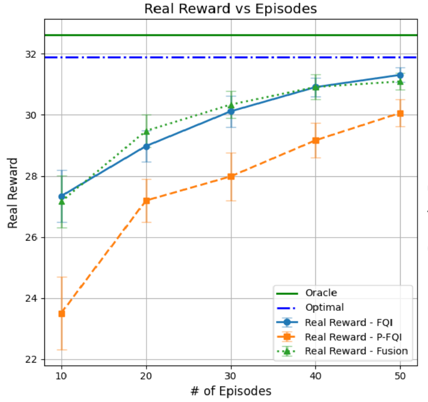
(a)

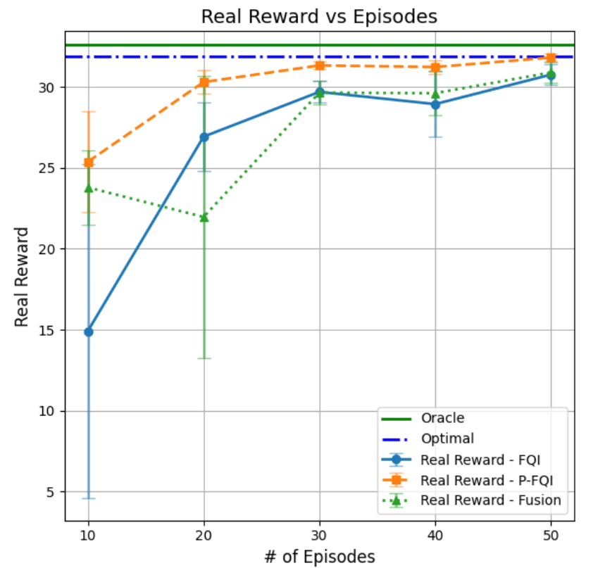
(b)

Figure 6: Convergence of the performances of the proposed algorithms to the optimal policy as the sample size increases: (a) Results under a uniform behavior policy; (b) Results under the optimal behavior policy. The performance of the oracle policy, $\pi^{\ast}_{\text{oracle}}$, and the optimal policy, $\pi^{\ast}$ are denoted by the green and dark blue horizontal line, respectively. The performance of C-FQI, PC-FQI and fusion of these two algorithms are denoted by light blue, orange and light green lines, respectively. The error bars represent 0.95 confidence intervals.

6 Conclusion

In this paper, we explore a sequential feature-based pricing and inventory control problem in an offline, data-driven context, where demand is censored and non-i.i.d. We discuss the challenges posed by the failure of the Markov property along with demand censoring in the observed data and propose solutions to address these issues in the development of efficient algorithms. Following this, we introduce two innovative, non-parametric data-driven algorithms that integrate techniques from survival analysis and offline RL. We derive their finite-sample regret guarantees and demonstrate their effectiveness through simulation experiments.

To conclude this paper, we highlight several avenues for future research. Our current focus has been on the joint pricing and inventory control problem of a single agent. However, supply chains typically involve multiple echelons, whose interactions significantly influence each other’s decisions regarding pricing and inventory. Thus, investigating the dynamics of competition and cooperation among supply chain echelons, both under the conditions of complete and incomplete information, presents a valuable area for further exploration. Additionally, our model assumes that decisions regarding inventory replenishment and pricing are made simultaneously at the start of each period, prior to the realization of demand. In real-world settings, firms often have the opportunity to adjust prices in response to observed demand information—a strategy known as ”responsive pricing.” Incorporating responsive pricing into our model represents an intriguing direction for future research, potentially offering deeper insights into how firms can dynamically adjust their strategies to optimize performance.

Appendix A Regret Decomposition

In this section, we present the derivation of the regret decomposition for a policy $\pi$, defined as follows:

$$\text{Regret}(\pi)={\cal V}(\pi^{\ast})-{\cal V}(\pi)\text{,}$$ (33)

where $\pi^{*}$ is the optimal policy defined in Equation (5). Firstly, we make several observations and state the necessary assumptions for deriving the regret decomposition.

Recall that the final estimated policies produced by C-FQI and Pessimistic C-FQI are of the form of the following:

$$\pi(a^{\prime}\,|\,H^{{}^{\prime}}_{(t-\hat{n}_{K,b}):t}) =\sum_{i=0}^{\min(t,\hat{n}_{K,b}-1)}\pi^{(i)}(a^{\prime}\mid H^{{}^{\prime}}_{(t-i):t})\prod_{j=1}^{i}\left\{\mathbb{I}[\Delta_{t-j}=0]\right\}\mathbb{I}[\Delta_{t-i-1}=1]$$

$$\quad+a_{\max}(H^{{}^{\prime}}_{(t-\hat{n}_{K,b}):t})\prod_{j=1}^{\hat{n}_{K,b}}\left\{\mathbb{I}[\Delta_{t-j}=0]\right\}\mathbb{I}[t\geq\hat{n}_{K,b}],$$ (34)

where $H^{{}^{\prime}}_{(t-i):t}=(W_{t},A_{t-1},\cdots,A_{t-i},W_{t-i})$ and $\hat{n}_{K,b}$ represents the maximum number of consecutive censoring instances observed within the window of length $K$ of the offline data across all trajectories. This form clearly shows that both policies, $\widehat{\pi}_{K}$ and $\widetilde{\pi}_{K}$, are implicitly a function of the offline data. Therefore, when considering value of the estimated final policies, data dependency needs to be taken into account. In addition, we have the following observation,

$${\cal V}(\pi)=\mathbb{E}_{\mathscr{O}_{N}}\left[\mathbb{E}^{\pi}\left[\sum_{t=0}^{\infty}\gamma^{t}R_{t}\,|\,\mathscr{O}_{N}\right]\right].$$

Next, we make the following assumption.

Assumption 8.

$\operatorname{Pr}^{\pi^{*}_{\mathscr{C}}}(\mathscr{C}(K,n_{K,b}))=1$, where $\pi^{*}_{\mathscr{C}}\in\text{argmax}_{\pi^{{}^{\prime}}\in\Pi}\mathbb{E}^{\pi^{{}^{\prime}}}\left[\sum_{t=0}^{\infty}\gamma^{t}R_{t}\,|\,\mathscr{C}(K,n_{K,b})\right]$

Now, we are ready to state the Lemma outlining the regret decomposition:

Lemma 4.

Under Assumptions 1, 3, 5 and 8 the regret of any policy, $\pi$, which belongs to $\Pi_{n_{K,b}}$ is given by:

$$\textup{Regret}(\pi) \leq\left(\sup_{\pi^{\prime}\in\Pi_{n_{K,b}}}\mathbb{E}^{\pi^{\prime}}\left[\sum_{t=0}^{\infty}\gamma^{t}R_{t}\right]-\mathbb{E}^{\pi}\left[\sum_{t=0}^{\infty}\gamma^{t}R_{t}\right]+2R_{\max}\frac{\gamma^{K+1}}{1-\gamma}\right)\operatorname{Pr}^{\pi^{*}}(\mathscr{C}(K,n_{K,b}))$$

$$\quad+(K-n_{K,b}+1)(1-\alpha_{\pi^{*},1})^{n_{K,b}}\left(\frac{2R_{\max}}{1-\gamma}\right)$$

$$\quad+\frac{4R_{\max}\sqrt{K-1}}{1-\gamma}\omega_{NT}$$

where $\mathscr{C}(K,n_{K,b})$ and $\Pi_{n_{K,b}}$ are characterized in Definitions 2 and 4 respectively.

Proof:

Recall that the probability of observing censoring in the next time step under policy $\pi$ given the last $n$ periods are censored is denoted by:

$$\operatorname{Pr}^{\pi}(\Delta_{t+1}=0\,|\,\Delta_{t}=\cdots=\Delta_{t-n+1}=0)=1-\alpha_{\pi,n}\text{ }\forall t\geq 0\text{.}$$

Let $\mathscr{B}_{i}$ represent the set containing all trajectories with sub-sequences that exhibit more than $n_{K,b}$ consecutive instances of censoring within the first $K$ horizon starting from the $i$-th decision point. Formally,

$$\mathscr{B}_{i}=\left\{\{W_{t},A_{t}\}_{t\geq 0}\mid\exists k>n_{K,b}\ \text{such that}\ \forall j\in\{i,\ldots,i+k-1\},\Delta_{j}=0,\text{ and }\ i+k-1<K\right\}$$

Under these definitions, $\operatorname{Pr}^{\pi}(\mathscr{B}_{i})$ can be bounded from above as follows:

$$\operatorname{Pr}^{\pi}(\mathscr{B}_{i}) =\operatorname{Pr}^{\pi}(\Delta_{i-1}=1,\Delta_{i}=0,\cdots,\Delta_{i+n_{K,b}}=0)$$

$$\leq\operatorname{Pr}^{\pi}(\Delta_{i}=0,\cdots,\Delta_{i+n_{K,b}}=0)$$

$$=\operatorname{Pr}^{\pi}(\Delta_{i}=0)\operatorname{Pr}^{\pi}(\Delta_{i+1}=0\,|\,\Delta_{i}=0)\cdots\operatorname{Pr}^{\pi}(\Delta_{i+n_{K,b}}=0\,|\,\Delta_{i+n_{K,b}-1}=\cdots=\Delta_{i}=0)$$

$$\leq\prod_{j=1}^{n_{K,b}}(1-\alpha_{\pi,j})\text{.}$$

Under Assumption 3, the probability of observing a non-censored state under the optimal policy increases as the number of consecutive censoring in the previous periods increases. This implies $1-\alpha_{\pi^{*},j}$ decreases as $j$ increases. Therefore,

$$\operatorname{Pr}^{\pi^{*}}(\mathscr{B}_{i})\leq(1-\alpha_{\pi^{*},1})^{n_{K,b}}.$$ (35)

Furthermore, it follows from Definition 2 and the definition of $\mathscr{B}_{i}$ that $\mathscr{C}^{c}(K,n_{K,b})=\cup_{i=0}^{K-n_{K,b}}\mathscr{B}_{i}$. Therefore, for any policy $\pi$, we have:

$$\operatorname{Pr}^{\pi}(\mathscr{C}^{c}(K,n_{K,b}))\leq\sum_{i=0}^{K-n_{K,b}}\operatorname{Pr}^{\pi}(\mathscr{B}_{i})\leq(K-n_{K,b}+1)\prod_{j=1}^{n_{K,b}}(1-\alpha_{\pi,j}).$$ (36)

Given Equations (35) and (36), it can be concluded that:

$$\operatorname{Pr}^{\pi^{*}}(\mathscr{C}^{c}(K,n_{K,b}))\leq(K-n_{K,b}+1)(1-\alpha_{\pi^{*},1})^{n_{K,b}}\text{.}$$ (37)

Recall that $n_{T^{\prime},b}$ and $\hat{n}_{T^{\prime},b}$ denote the maximum number of consecutive censoring that can be observed and is observed in the windows with length $T^{\prime}$ under the data distribution and in the offline data, respectively. Therefore, $\hat{n}_{T^{\prime},b}$ serves as an estimator for $n_{T^{\prime},b}$. Furthermore, $\hat{n}_{T^{\prime},b}\xrightarrow{P}n_{T^{\prime},b}$ under Assumption 5.

Next, we propose to decompose the regret using the law of iterated expectations as follows:

$$\text{Regret}(\pi) ={\cal V}(\pi^{*})-{\cal V}(\pi)$$

$$=\mathbb{E}^{\pi^{*}}\left[\sum_{t=0}^{\infty}\gamma^{t}R_{t}\right]-\mathbb{E}_{\mathscr{O}_{N}}\left[\mathbb{E}^{\pi}\left[\sum_{t=0}^{\infty}\gamma^{t}R_{t}\,|\,\mathscr{O}_{N}\right]\right]$$

$$=\mathbb{E}_{\mathscr{O}_{N}}\left[\mathbb{E}^{\pi^{*}}\left[\sum_{t=0}^{\infty}\gamma^{t}R_{t}\,|\,\mathscr{O}_{N}\right]-\mathbb{E}^{\pi}\left[\sum_{t=0}^{\infty}\gamma^{t}R_{t}\,|\,\mathscr{O}_{N}\right]\right]$$

$$=\mathbb{E}_{\mathscr{O}_{N}}\left\{\mathbb{E}^{\pi^{*}}\left[\sum_{t=0}^{\infty}\gamma^{t}R_{t}\mid\mathscr{C}(K,\hat{n}_{K,b}),\mathscr{O}_{N}\right]\operatorname{Pr}^{\pi^{*}}(\mathscr{C}(K,\hat{n}_{K,b})\mid\mathscr{O}_{N})\right.$$

$$\quad\left.+\mathbb{E}^{\pi^{*}}\left[\sum_{t=0}^{\infty}\gamma^{t}R_{t}\mid\mathscr{C}^{c}(K,\hat{n}_{K,b}),\mathscr{O}_{N}\right]\operatorname{Pr}^{\pi^{*}}(\mathscr{C}^{c}(K,\hat{n}_{K,b})\mid\mathscr{O}_{N})\right.$$

$$\quad\left.-\mathbb{E}^{\pi}\left[\sum_{t=0}^{\infty}\gamma^{t}R_{t}\mid\mathscr{C}(K,\hat{n}_{K,b}),\mathscr{O}_{N}\right]\operatorname{Pr}^{\pi}(\mathscr{C}(K,\hat{n}_{K,b})\mid\mathscr{O}_{N})\right.$$

$$\quad\left.-\mathbb{E}^{\pi}\left[\sum_{t=0}^{\infty}\gamma^{t}R_{t}\mid\mathscr{C}^{c}(K,\hat{n}_{K,b}),\mathscr{O}_{N}\right]\operatorname{Pr}^{\pi}(\mathscr{C}^{c}(K,\hat{n}_{K,b})\mid\mathscr{O}_{N})\right\}$$

$$=\sum_{m=0}^{K}\operatorname{Pr}^{\pi^{b}}(\hat{n}_{K,b}=m)\left\{\mathbb{E}^{\pi^{*}}\left[\sum_{t=0}^{\infty}\gamma^{t}R_{t}\mid\mathscr{C}(K,m)\right]\operatorname{Pr}^{\pi^{*}}(\mathscr{C}(K,m))\right.$$

$$\quad\left.+\mathbb{E}^{\pi^{*}}\left[\sum_{t=0}^{\infty}\gamma^{t}R_{t}\mid\mathscr{C}^{c}(K,m)\right]\operatorname{Pr}^{\pi^{*}}(\mathscr{C}^{c}(K,m))\right.$$

$$\quad\left.-\mathbb{E}^{\pi}\left[\sum_{t=0}^{\infty}\gamma^{t}R_{t}\mid\mathscr{C}(K,m)\right]\operatorname{Pr}^{\pi}(\mathscr{C}(K,m))\right.$$

$$\quad\left.-\mathbb{E}^{\pi}\left[\sum_{t=0}^{\infty}\gamma^{t}R_{t}\mid\mathscr{C}^{c}(K,m)\right]\operatorname{Pr}^{\pi}(\mathscr{C}^{c}(K,m))\right\},$$

where we leverage the fact that only $\hat{n}_{K,b}$ is dependent on the offline data, whereas both $\pi^{\ast}$ and $\pi$ are independent of it, with the independence of $\pi$ contingent upon a fixed $\hat{n}_{K,b}$.

Following this, we decompose the summation into two parts as follows:

$$\text{Regret}(\pi) =\operatorname{Pr}^{\pi^{b}}(\hat{n}_{K,b}=n_{K,b})\left\{\mathbb{E}^{\pi^{*}}\left[\sum_{t=0}^{\infty}\gamma^{t}R_{t}\mid\mathscr{C}(K,n_{K,b})\right]\operatorname{Pr}^{\pi^{*}}(\mathscr{C}(K,n_{K,b}))\right.$$

$$\left.\quad+\mathbb{E}^{\pi^{*}}\left[\sum_{t=0}^{\infty}\gamma^{t}R_{t}\mid\mathscr{C}^{c}(K,n_{K,b})\right]\operatorname{Pr}^{\pi^{*}}(\mathscr{C}^{c}(K,n_{K,b}))\right.$$

$$\left.\quad-\mathbb{E}^{\pi}\left[\sum_{t=0}^{\infty}\gamma^{t}R_{t}\mid\mathscr{C}(K,n_{K,b})\right]\operatorname{Pr}^{\pi}(\mathscr{C}(K,n_{K,b}))\right.$$

$$\left.\quad-\mathbb{E}^{\pi}\left[\sum_{t=0}^{\infty}\gamma^{t}R_{t}\mid\mathscr{C}^{c}(K,n_{K,b})\right]\operatorname{Pr}^{\pi}(\mathscr{C}^{c}(K,n_{K,b}))\right\}$$

$$+\sum_{m\neq n_{K,b}}\operatorname{Pr}^{\pi^{b}}(\hat{n}_{K,b}=m)\left\{\mathbb{E}^{\pi^{*}}\left[\sum_{t=0}^{\infty}\gamma^{t}R_{t}\mid\mathscr{C}(K,m)\right]\operatorname{Pr}^{\pi^{*}}(\mathscr{C}(K,m))\right.$$

$$\left.\quad+\mathbb{E}^{\pi^{*}}\left[\sum_{t=0}^{\infty}\gamma^{t}R_{t}\mid\mathscr{C}^{c}(K,m)\right]\operatorname{Pr}^{\pi^{*}}(\mathscr{C}^{c}(K,m))\right.$$

$$\left.\quad-\mathbb{E}^{\pi}\left[\sum_{t=0}^{\infty}\gamma^{t}R_{t}\mid\mathscr{C}(K,m)\right]\operatorname{Pr}^{\pi}(\mathscr{C}(K,m))\right.$$

$$\left.\quad-\mathbb{E}^{\pi}\left[\sum_{t=0}^{\infty}\gamma^{t}R_{t}\mid\mathscr{C}^{c}(K,m)\right]\operatorname{Pr}^{\pi}(\mathscr{C}^{c}(K,m))\right\}.$$ (38)

Consider the first part where $\hat{n}_{K,b}=n_{K,b}$. Equation (A) implies that $\pi\in\Pi_{n_{K,b}}$ in the first part of the summation. Therefore, $\mathscr{C}(K,n_{K,b})$ is a sure event under $\pi$. Next, consider the second part based on which we define $a_{m}$ and $b_{m}$ as

$$a_{m}=\operatorname{Pr}^{\pi^{b}}(\hat{n}_{K,b}=m)$$

$$b_{m} =\mathbb{E}^{\pi^{*}}\left[\sum_{t=0}^{\infty}\gamma^{t}R_{t}\mid\mathscr{C}(K,m)\right]\operatorname{Pr}^{\pi^{*}}(\mathscr{C}(K,m))+\mathbb{E}^{\pi^{*}}\left[\sum_{t=0}^{\infty}\gamma^{t}R_{t}\mid\mathscr{C}^{c}(K,m)\right]\operatorname{Pr}^{\pi^{*}}(\mathscr{C}^{c}(K,m))$$

$$\quad-\mathbb{E}^{\pi}\left[\sum_{t=0}^{\infty}\gamma^{t}R_{t}\mid\mathscr{C}(K,m)\right]\operatorname{Pr}^{\pi}(\mathscr{C}(K,m))-\mathbb{E}^{\pi}\left[\sum_{t=0}^{\infty}\gamma^{t}R_{t}\mid\mathscr{C}^{c}(K,m)\right]\operatorname{Pr}^{\pi}(\mathscr{C}^{c}(K,m))$$

Following this, we note that $\sum_{m\neq n_{K,b}}a_{m}\leq\omega_{NT}$, and therefore, $\sum_{m\neq n_{K,b}}a_{m}^{2}\leq\omega_{NT}^{2}$, as implied by Assumption 5. Additionally, since $b_{m}\leq\frac{4R_{\max}}{1-\gamma}$, we have $\sum_{m\neq n_{K,b}}b_{m}^{2}\leq(K-1)\left(\frac{4R_{\max}}{1-\gamma}\right)^{2}$, given that $|R_{t}|\leq R_{\max}$ for all $t\geq 0$. Then, by applying the Cauchy-Schwarz inequality, it follows that

$$\sum_{m\neq n_{K,b}}a_{m}b_{m}\leq\frac{4R_{\max}\sqrt{K-1}}{1-\gamma}\omega_{NT}$$

Therefore, the upper bound on the regret is expressed as:

$$\text{Regret}(\pi) \leq\operatorname{Pr}^{\pi^{b}}(\hat{n}_{K,b}=n_{K,b})\left\{\left(\mathbb{E}^{\pi^{*}}\left[\sum_{t=0}^{\infty}\gamma^{t}R_{t}\mid\mathscr{C}(K,n_{K,b})\right]-\mathbb{E}^{\pi}\left[\sum_{t=0}^{\infty}\gamma^{t}R_{t}\right]\right)\operatorname{Pr}^{\pi^{*}}(\mathscr{C}(K,n_{K,b}))\right.$$

$$\left.\quad+\left(\mathbb{E}^{\pi^{*}}\left[\sum_{t=0}^{\infty}\gamma^{t}R_{t}\mid\mathscr{C}^{c}(K,n_{K,b})\right]-\mathbb{E}^{\pi}\left[\sum_{t=0}^{\infty}\gamma^{t}R_{t}\right]\right)\operatorname{Pr}^{\pi^{*}}(\mathscr{C}^{c}(K,n_{K,b}))\right\}$$

$$\quad+\frac{4R_{\max}\sqrt{K-1}}{1-\gamma}\omega_{NT},$$ (39)

Next, we use Equation (37) and the fact that $|R_{t}|\leq R_{\max}$ $\forall t\geq 0$ to obtain the following:

$$\text{Regret}(\pi) \leq\operatorname{Pr}^{\pi^{b}}(\hat{n}_{K,b}=n_{K,b})\left\{\left(\mathbb{E}^{\pi^{*}}\left[\sum_{t=0}^{\infty}\gamma^{t}R_{t}\mid\mathscr{C}(K,n_{K,b})\right]-\mathbb{E}^{\pi}\left[\sum_{t=0}^{\infty}\gamma^{t}R_{t}\right]\right)\operatorname{Pr}^{\pi^{*}}(\mathscr{C}(K,n_{K,b}))\right\}$$

$$\quad+(K-n_{K,b}+1)(1-\alpha_{\pi^{*},1})^{n_{K,b}}\left(\frac{2R_{\max}}{1-\gamma}\right)$$

$$\quad+\frac{4R_{\max}\sqrt{K-1}}{1-\gamma}\omega_{NT}$$ (40)

Observe that by definition, $\pi^{*}$ is the optimal policy that maximizes $\mathbb{E}^{\pi}\left[\sum_{t=0}^{\infty}\gamma^{t}R_{t}\right]$. However, it does not necessarily remain optimal for $\mathbb{E}^{\pi}\left[\sum_{t=0}^{\infty}\gamma^{t}R_{t}\,|\,\mathscr{C}(K,n_{K,b})\right]$ as the transition probabilities are altered once conditioned on $\mathscr{C}(K,n_{K,b})$. We denote by $\pi^{*}_{\mathscr{C}}$ the optimal policy under the event $\mathscr{C}(K,n_{K,b})$ (i.e $\pi^{*}_{\mathscr{C}}\in\text{argmax}_{\pi^{{}^{\prime}}\in\Pi}\mathbb{E}^{\pi^{{}^{\prime}}}\left[\sum_{t=0}^{\infty}\gamma^{t}R_{t}\,|\,\mathscr{C}(K,n_{K,b})\right]$). Given the optimality of $\pi^{*}_{\mathscr{C}}$, it follows that $\mathbb{E}^{\pi^{{}^{\prime}}}\left[\sum_{t=0}^{\infty}\gamma^{t}R_{t}\,|\,\mathscr{C}(K,n_{K,b})\right]\leq\mathbb{E}^{\pi_{\mathscr{C}}^{*}}\left[\sum_{t=0}^{\infty}\gamma^{t}R_{t}\,|\,\mathscr{C}(K,n_{K,b})\right]$ $\forall\pi^{{}^{\prime}}\in\Pi$. Consequently, the upper bound on the regret can be further expressed as:

$$\text{Regret}(\pi) \leq\left(\mathbb{E}^{\pi_{\mathscr{C}}^{*}}\left[\sum_{t=0}^{\infty}\gamma^{t}R_{t}\mid\mathscr{C}(K,n_{K,b})\right]-\mathbb{E}^{\pi}\left[\sum_{t=0}^{\infty}\gamma^{t}R_{t}\right]\right)\operatorname{Pr}^{\pi^{*}}(\mathscr{C}(K,n_{K,b}))$$

$$\quad+(K-n_{K,b}+1)(1-\alpha_{\pi^{*},1})^{n_{K,b}}\left(\frac{2R_{\max}}{1-\gamma}\right)$$

$$\quad+\frac{4R_{\max}\sqrt{K-1}}{1-\gamma}\omega_{NT}$$ (41)

Consider the following term $\forall\pi\in\Pi_{n_{K,b}}$:

$$\mathbb{E}^{\pi_{\mathscr{C}}^{*}}\left[\sum_{t=0}^{\infty}\gamma^{t}R_{t}\,|\,\mathscr{C}(K,n_{K,b})\right] =\mathbb{E}^{\pi_{\mathscr{C}}^{*}}\left[\sum_{t=0}^{K}\gamma^{t}R_{t}\,|\,\mathscr{C}(K,n_{K,b})\right]+\mathbb{E}^{\pi_{\mathscr{C}}^{*}}\left[\sum_{t=K+1}^{\infty}\gamma^{t}R_{t}\,|\,\mathscr{C}(K,n_{K,b})\right]$$

$$\leq\mathbb{E}^{\pi_{\mathscr{C}}^{*}}\left[\sum_{t=0}^{K}\gamma^{t}R_{t}\,|\,\mathscr{C}(K,n_{K,b})\right]+\mathbb{E}^{\pi}\left[\sum_{t=K+1}^{\infty}\gamma^{t}R_{t}\,|\,\mathscr{C}(K,n_{K,b})\right]$$

$$+2R_{\max}\frac{\gamma^{K+1}}{1-\gamma}$$

$$=\mathbb{E}^{\pi_{\mathscr{C}}^{*}}\left[\sum_{t=0}^{K}\gamma^{t}R_{t}\right]+\mathbb{E}^{\pi}\left[\sum_{t=K+1}^{\infty}\gamma^{t}R_{t}\right]$$

$$+2R_{\max}\frac{\gamma^{K+1}}{1-\gamma},$$ (42)

where the last equality follows from the fact that $\mathscr{C}(K,n_{K,b})$ is a sure event under $\pi^{\ast}_{\mathscr{C}}$, as implied by Assumption 8, and from the condition that $\pi\in\Pi_{n_{K,b}}$.

Next, note that $\pi_{\mathscr{C}}^{\ast}$ results in at most $n_{K,b}$ consecutive censorings within the first $K$ steps, while $\pi$ results in at most $n_{K,b}$ consecutive censoring over the entire horizon. Based on this, we define a policy, denoted by $\pi_{n_{K,b}}$, as $\pi^{\ast}{\mathscr{C}}\mathbb{I}[t\leq K]+\pi\mathbb{I}[t>K]$. This policy ensures at most $n_{K,b}$ consecutive censoring across the entire horizon. Therefore,

$$\mathbb{E}^{\pi_{\mathscr{C}}^{*}}\left[\sum_{t=0}^{K}\gamma^{t}R_{t}\right]+\mathbb{E}^{\pi}\left[\sum_{t=K+1}^{\infty}\gamma^{t}R_{t}\right] =\mathbb{E}^{\pi_{n_{K,b}}}\left[\sum_{t=0}^{K}\gamma^{t}R_{t}\right]$$

$$\leq\sup_{\pi^{\prime}\in\Pi_{n_{K,b}}}\mathbb{E}^{\pi^{\prime}}\left[\sum_{t=0}^{\infty}\gamma^{t}R_{t}\right].$$

This implies

$$\mathbb{E}^{\pi_{\mathscr{C}}^{*}}\left[\sum_{t=0}^{\infty}\gamma^{t}R_{t}\,|\,\mathscr{C}(K,n_{K,b})\right]\leq\sup_{\pi^{\prime}\in\Pi_{n_{K,b}}}\mathbb{E}^{\pi^{\prime}}\left[\sum_{t=0}^{\infty}\gamma^{t}R_{t}\right]+2R_{\max}\frac{\gamma^{K+1}}{1-\gamma}.$$ (43)

Therefore, the upper bound on the regret becomes the following:

$$\text{Regret}(\pi) \leq\left(\sup_{\pi^{\prime}\in\Pi_{n_{K,b}}}\mathbb{E}^{\pi^{\prime}}\left[\sum_{t=0}^{\infty}\gamma^{t}R_{t}\right]-\mathbb{E}^{\pi}\left[\sum_{t=0}^{\infty}\gamma^{t}R_{t}\right]+2R_{\max}\frac{\gamma^{K+1}}{1-\gamma}\right)\operatorname{Pr}^{\pi^{*}}(\mathscr{C}(K,n_{K,b}))$$

$$\quad+(K-n_{K,b}+1)(1-\alpha_{\pi^{*},1})^{n_{K,b}}\left(\frac{2R_{\max}}{1-\gamma}\right)$$

$$\quad+\frac{4R_{\max}\sqrt{K-1}}{1-\gamma}\omega_{NT}.$$ (44)

This concludes the proof of Lemma 4.

Appendix B Proof of Regret Bound for C-FQI given Theorem 1

In this section, we provide the proof of Theorem 1 which develops an upper bound on the regret of the policy $\widehat{\pi}_{K}$ produced by C-FQI.

Since $\widehat{\pi}_{K}$ is of the form of Equation (A), we can apply Lemma 4 which states that

$$\text{Regret}(\widehat{\pi}_{K}) \leq\left(\underbrace{\sup_{\pi^{\prime}\in\Pi_{n_{K,b}}}\mathbb{E}^{\pi^{\prime}}\left[\sum_{t=0}^{\infty}\gamma^{t}R_{t}\right]-\mathbb{E}^{\widehat{\pi}_{K}}\left[\sum_{t=0}^{\infty}\gamma^{t}R_{t}\right]}_{(i)}+2R_{\max}\frac{\gamma^{K+1}}{1-\gamma}\right)\operatorname{Pr}^{\pi^{*}}(\mathscr{C}(K,n_{K,b}))$$ (45)

$$\quad+(K-n_{K,b}+1)(1-\alpha_{\pi^{*},1})^{n_{K,b}}\left(\frac{2R_{\max}}{1-\gamma}\right)$$

$$\quad+\frac{4R_{\max}\sqrt{K-1}}{1-\gamma}\omega_{N}.$$ (46)

Therefore, it remains to upper bound the term $(i)$.

By Lemma 13, we know that $\pi^{\ast}_{n_{K,b}}\in\text{argmax}_{\pi^{\prime}\in\Pi_{n_{K,b}}}\mathbb{E}^{\pi^{\prime}}\left[\sum_{t=0}^{\infty}\gamma^{t}R_{t}\right]$. Furthermore, we can apply Lemma 8 as both $\pi^{\ast}_{n_{K,b}}$ and $\widehat{\pi}_{K}$ belong to $\Pi_{n_{K,b}}$ by construction. This implies the following:

$$(i) =\mathbb{E}^{\pi^{\ast}_{n_{K,b}}}\left[\sum_{t=0}^{\infty}\gamma^{t}R_{t}\right]-\mathbb{E}^{\widehat{\pi}_{K}}\left[\sum_{t=0}^{\infty}\gamma^{t}R_{t}\right]$$ (47)

$$=\frac{1-\gamma^{n_{K,b}}}{(1-\gamma)^{2}}\mathbb{E}_{(W^{(0)},A^{(0)},\cdots,W^{(I)},A^{(I)})\sim d_{\nu,I}^{\widehat{\pi}_{K}}\times\widehat{\pi}_{K}}\left[-A^{(I)}_{\pi^{\ast}_{n_{K,b}},\mathscr{C}}(W^{(0)},A^{(0)},\cdots,W^{(I)},A^{(I)})\prod_{j=1}^{I}\left\{\mathbb{I}[\Delta^{(j)}=0]\right\}\mathbb{I}[\Delta^{(0)}=1]\right],$$

where $\nu$ is the reference distribution on the initial state and known by the decision maker, $I$ is the discrete random variable given in Definition 21 and $d^{\widehat{\pi}_{K}}_{\nu,i}$ is the state action visitation measure under $\widehat{\pi}_{K}$, given in Definition 20 for the tuple $(W^{(0)},A^{(0)},\cdots,W^{(I)})$.

Assume that by conditioning on $I=i$ and the sequence $(W^{(0)},A^{(0)},\dots,W^{(i)})=(w^{(0)},a^{(0)},\dots,w^{(i)})$, where $\Delta^{(0)}=1$ and $\Delta^{(j)}=0$ for all $j=1,\dots,i$, the expectation above can be upper bounded for all $i=0,\dots,n_{K,b}-1$ as follows:

$$-A^{(i)}_{\pi^{\ast}_{n_{K,b}},\mathscr{C}}(w^{(0)},a^{(0)},\cdots,w^{(i)},\widehat{\pi}^{(i)}(w^{(i)},\cdots,w^{(0)},a^{(0)}))$$

$$=Q^{(i)}_{\pi^{\ast}_{n_{K,b}},\mathscr{C}}(w^{(0)},a^{(0)},\cdots,w^{(i)},\pi^{(i)}_{n_{K,b},*}(w^{(i)},\cdots,w^{(0)},a^{(0)})-Q^{(i)}_{\pi^{\ast}_{n_{K,b}},\mathscr{C}}(w^{(0)},a^{(0)},\cdots,w^{(i)},\widehat{\pi}^{(i)}_{K}(w^{(i)},\cdots,w^{(0)},a^{(0)})$$

$$\leq Q^{(i)}_{\pi^{\ast}_{n_{K,b}},\mathscr{C}}(w^{(0)},a^{(0)},\cdots,w^{(i)},\pi^{(i)}_{n_{K,b},*}(w^{(i)},\cdots,w^{(0)},a^{(0)})-\widehat{Q}^{(i)}_{K}(w^{(0)},a^{(0)},\cdots,w^{(i)},\pi^{(i)}_{n_{K,b},*}(w^{(i)},\cdots,w^{(0)},a^{(0)}))$$

$$+\widehat{Q}^{(i)}_{K}(w^{(0)},a^{(0)},\cdots,w^{(i)},\widehat{\pi}^{(i)}_{K}(s^{(i)},\cdots,w^{(0)},a^{(0)})-Q^{(i)}_{\pi^{\ast}_{n_{K,b}},\mathscr{C}}(w^{(0)},a^{(0)},\cdots,w^{(i)},\widehat{\pi}^{(i)}_{K}(w^{(i)},\cdots,w^{(0)},a^{(0)}),$$ (48)

where the inequality stems from the optimality of $\widehat{\pi}_{K}$ on $\widehat{Q}^{(i)}_{K}$ $\forall i=0,\dots,n_{K,b}-1$.

For $i=n_{K,b}$, the policy $\widehat{\pi}_{K}$ no longer maintains its optimality with respect to $\widehat{Q}^{(n_{K,b})}_{K}$ as it picks $a_{\max}$ given in Assumption 2. Consequently, the inequality specified in Equation (B) is not applicable when $i=n_{K,b}$. To quantify the optimality gap, let

$$\textup{AD}^{\widehat{\pi}_{K}}(w^{(0)},a^{(0)},\cdots,w^{(n_{K,b})})$$ (49)

$$=\max_{a\in{\cal A}}\widehat{Q}_{K}^{(n_{K,b})}(w^{(0)},a^{(0)},\cdots,w^{(n_{K,b})},a)-\widehat{Q}_{K}^{(n_{K,b})}(w^{(0)},a^{(0)},\cdots,w^{(n_{K,b})},\widehat{\pi}_{K}^{(n_{K,b})}(w^{(n_{K,b})},\cdots,w^{(0)},a^{(0)})).$$

It is worth noting that this constant can be computed straightforwardly. Hence, with this optimality gap, we can upper bound $-A^{(n_{K,b})}_{\pi^{\ast}_{n_{K,b},\mathscr{C}}}$ as follows:

$$-A^{(n_{K,b})}_{\pi^{\ast}_{n_{K,b}},\mathscr{C}}(w^{(0)},a^{(0)},\cdots,w^{(n_{K,b})},\widehat{\pi}_{K}^{(n_{K,b})}(w^{(n_{K,b})},\cdots,w^{(0)},a^{(0)}))$$

$$=Q^{(n_{K,b})}_{\pi^{\ast}_{n_{K,b}},\mathscr{C}}(w^{(0)},a^{(0)},\cdots,w^{(n_{K,b})},\pi^{(n_{K,b})}_{n_{K,b},\ast}(w^{(n_{K,b})},\cdots,w^{(0)},a^{(0)})-\max_{a\in{\cal A}}\widehat{Q}^{(n_{K,b})}_{K}(w^{(0)},a^{(0)},\cdots,w^{(n_{K,b})},a)$$

$$+\max_{a\in{\cal A}}\widehat{Q}^{(n_{K,b})}_{K}(w^{(0)},a^{(0)},\cdots,w^{(n_{K,b})},a)-Q^{(n_{K,b})}_{\pi^{\ast}_{n_{K,b}},\mathscr{C}}(w^{(0)},a^{(0)},\cdots,w^{(n_{K,b})},\widehat{\pi}^{(n_{K,b})}_{K}(w^{(n_{K,b})},\cdots,w^{(0)},a^{(0)}))$$

$$\leq Q^{(n_{K,b})}_{\pi^{\ast}_{n_{K,b}},\mathscr{C}}(w^{(0)},a^{(0)},\cdots,w^{(n_{K,b})},\pi^{(n_{K,b})}_{n_{K,b},\ast}(w^{(n_{K,b})},\cdots,w^{(0)},a^{(0)})$$

$$-\widehat{Q}^{(n_{K,b})}_{K}(w^{(0)},a^{(0)},\cdots,w^{(n_{K,b})},\pi^{(n_{K,b})}_{n_{K,b},\ast}(w^{(n_{K,b})},\cdots,w^{(0)},a^{(0)}))$$

$$+\widehat{Q}^{(n_{K,b})}_{K}(w^{(0)},a^{(0)},\cdots,w^{(n_{K,b})},\widehat{\pi}^{(n_{K,b})}_{K}(w^{(n_{K,b})},\cdots,w^{(0)},a^{(0)}))$$

$$-Q^{(n_{K,b})}_{\pi^{\ast}_{n_{K,b}},\mathscr{C}}(w^{(0)},a^{(0)},\cdots,w^{(n_{K,b})},\widehat{\pi}^{(n_{K,b})}_{K}(w^{(n_{K,b})},\cdots,w^{(0)},a^{(0)}))$$

$$+\textup{AD}^{\widehat{\pi}_{K}}(w^{(0)},a^{(0)},\cdots,w^{(n_{K,b})}),$$ (50)

where first inequality comes from Equation (49) and the fact that

$$\max_{a\in{\cal A}}\widehat{Q}^{(n_{K,b})}_{K}(w^{(0)},a^{(0)},\cdots,w^{(n_{K,b})},a)\geq\widehat{Q}^{(n_{K,b})}_{K}(w^{(0)},a^{(0)},\cdots,w^{(n_{K,b})},\widehat{\pi}^{(n_{K,b})}_{*}(w^{(n_{K,b})},\cdots,w^{(0)},a^{(0)})).$$

By combining Equations (B) and (B), we have the following $\forall i=0,\cdots,n_{K,b}$:

$$-A^{(i)}_{\pi^{\ast}_{n_{K,b}},\mathscr{C}}(w^{(0)},a^{(0)},\cdots,w^{(i)},\widehat{\pi}^{(i)}(w^{(i)},\cdots,w^{(0)},a^{(0)}))$$

$$\leq Q^{(i)}_{\pi^{\ast}_{n_{K,b}},\mathscr{C}}(w^{(0)},a^{(0)},\cdots,w^{(i)},\pi^{(i)}_{n_{K,b},\ast}(w^{(i)},\cdots,w^{(0)},a^{(0)})-\widehat{Q}^{(i)}_{K}(w^{(0)},a^{(0)},\cdots,w^{(i)},\pi^{(i)}_{n_{K,b},\ast}(w^{(i)},\cdots,w^{(0)},a^{(0)}))$$

$$+\widehat{Q}^{(i)}_{K}(w^{(0)},a^{(0)},\cdots,w^{(i)},\widehat{\pi}^{(i)}_{K}(w^{(i)},\cdots,w^{(0)},a^{(0)})-Q^{(i)}_{\pi^{\ast}_{n_{K,b}},\mathscr{C}}(w^{(0)},a^{(0)},\cdots,w^{(i)},\widehat{\pi}^{(i)}_{K}(w^{(i)},\cdots,w^{(0)},a^{(0)}))$$

$$+\textup{AD}^{\widehat{\pi}_{K}}(w^{(0)},a^{(0)},\cdots,w^{(i)})\mathbb{I}[i=n_{K,b}].$$ (51)

Recall that

$$\overline{Q}^{(i)}_{K}(w^{(0)},a^{(0)},\cdots,w^{(i)},a^{(i)})=\widehat{Q}^{(i)}_{K}(w^{(0)},a^{(0)},\cdots,w^{(i)},a^{(i)})-C^{(i)}(w^{(0)},a^{(0)},\cdots,w^{(i)}),$$ (52)

where the exact definition of $\overline{Q}_{j}$ $\forall j=0,\cdots,K$ is given in Equation (107) and the characterization of $C^{(i)}(w^{(0)},a^{(0)},\cdots,w^{(i)})$ is given in Definition 18.

Next, we add and subtract $C^{(i)}(w^{(0)},a^{(0)},\cdots,w^{(i)})$ to the right hand side of Equation (B) to obtain $\overline{Q}^{(i)}$. This implies the following:

$$-A^{(i)}_{\pi^{\ast}_{n_{K,b}},\mathscr{C}}(w^{(0)},a^{(0)},\cdots,w^{(i)},\widehat{\pi}^{(i)}(w^{(i)},\cdots,w^{(0)},a^{(0)}))$$

$$\leq Q^{(i)}_{\pi^{\ast}_{n_{K,b}},\mathscr{C}}(w^{(0)},a^{(0)},\cdots,w^{(i)},\pi^{(i)}_{n_{K,b},\ast}(w^{(i)},\cdots,w^{(0)},a^{(0)})-\overline{Q}^{(i)}_{K}(w^{(0)},a^{(0)},\cdots,w^{(i)},\pi^{(i)}_{n_{K,b},\ast}(w^{(i)},\cdots,w^{(0)},a^{(0)}))$$

$$+\overline{Q}^{(i)}_{K}(w^{(0)},a^{(0)},\cdots,w^{(i)},\widehat{\pi}^{(i)}_{K}(w^{(i)},\cdots,w^{(0)},a^{(0)})-Q^{(i)}_{\pi^{\ast}_{n_{K,b}},\mathscr{C}}(w^{(0)},a^{(0)},\cdots,w^{(i)},\widehat{\pi}^{(i)}_{K}(w^{(i)},\cdots,w^{(0)},a^{(0)}))$$

$$+\textup{AD}^{\widehat{\pi}_{K}}(w^{(0)},a^{(0)},\cdots,w^{(i)})\mathbb{I}[i=n_{K,b}].$$ (53)

In order to upper bound the right hand side of Equation (B), we make use of Lemmas 9 and 10, which give an upper and lower bound on the following difference, $\forall i=0,\cdots,n_{K,b}$:

$$Q^{(i)}_{\pi^{\ast}_{n_{K,b}},\mathscr{C}}(w^{(0)},a^{(0)},\cdots,w^{(i)},a^{(i)})-\overline{Q}^{(i)}_{K}(w^{(0)},a^{(0)},\cdots,w^{(i)},a^{(i)}).$$ (54)

Specifically, under Lemmas 9 and 10, we have the following inequalities:

$$Q^{(i)}_{\pi^{\ast}_{n_{K,b}},\mathscr{C}}(w^{(0)},a^{(0)},\cdots,w^{(i)},a^{(i)})-\overline{Q}^{(i)}_{K}(w^{(0)},a^{(0)},\cdots,w^{(i)},a^{(i)})$$

$$\leq\gamma^{K-1}\left(\frac{2-\gamma}{1-\gamma}R_{\max}\right)+\textup{RD}(NT)$$

$$+\textup{UQ}(w^{(0)},a^{(0)}\cdots,w^{(i)},a^{(i)})+C^{(i)}(w^{(0)},a^{(0)}\cdots,w^{(i)})$$

and

$$Q^{(i)}_{\pi^{\ast}_{n_{K,b}},\mathscr{C}}(w^{(0)},a^{(0)},\cdots,w^{(i)},a^{(i)})-\overline{Q}^{(i)}_{K}(w^{(0)},a^{(0)},\cdots,w^{(i)},a^{(i)})$$

$$\geq-\gamma^{K-1}\left(\frac{2-\gamma}{1-\gamma}R_{\max}\right)-\textup{RD}(NT)-\textup{TAD}(w^{(0)},a^{(0)}\cdots,w^{(i)},a^{(i)}).$$

Hence, we can show that $\forall i=0,\cdots,n_{K,b}$:

$$-A^{(i)}_{\pi^{\ast}_{n_{K,b}},\mathscr{C}}(w^{(0)},a^{(0)},\cdots,\widehat{\pi}_{K}^{(i)}(w^{(i)},\cdots,w^{(0)},a^{(0)}))$$

$$\leq\text{UQ}(w^{(0)},a^{(0)},\cdots,w^{(i)},\pi^{(i)}_{n_{K,b},\ast}(w^{(i)},\cdots,w^{(0)},a^{(0)}))$$

$$+\textup{TAD}(w^{(0)},a^{(0)},\cdots,w^{(i)},\widehat{\pi}^{(i)}_{K}(w^{(i)},\cdots,w^{(0)},a^{(0)}))$$

$$+C^{(i)}(w^{(0)},a^{(0)},\cdots,w^{(i)})+2\gamma^{K-1}\left(\frac{2-\gamma}{1-\gamma}R_{\max}\right)+2\text{RD}(NT)$$

$$+\textup{AD}^{\widehat{\pi}_{K}}(w^{(0)},a^{(0)},\cdots,w^{(i)})\mathbb{I}[i=n_{K,b}].$$ (55)

Consequently, an upper bound on the term $(i)$ from Equation (47) can be established based on Equation (B) as follows:

$$(i) =\frac{1-\gamma^{n_{K,b}}}{(1-\gamma)^{2}}\mathbb{E}_{(W^{(0)},A^{(0)},\cdots,W^{(I)},A^{(I)})\sim d_{\nu,\mathscr{C},I}^{\widehat{\pi}_{K}}\times\widehat{\pi}_{K}}\left[-A^{(I)}_{\pi^{\ast}_{n_{K,b}},\mathscr{C}}(W^{(0)},A^{(0)},\cdots,W^{(I)},A^{(I)})\prod_{j=1}^{I}\left\{\mathbb{I}[\Delta^{(j)}=0]\right\}\mathbb{I}[\Delta^{(0)}=1]\right]$$

$$\leq\frac{1-\gamma^{n_{K,b}}}{(1-\gamma)^{2}}\mathbb{E}_{(W^{(0)},A^{(0)},\cdots,W^{(I)},A^{(I)})\sim d_{\nu,\mathscr{C},I}^{\widehat{\pi}_{K}}}\left[\left(\mathbb{E}^{\pi^{\ast}_{n_{K,b}}}\left[\text{UQ}(W^{(0)},A^{(0)},\cdots W^{(I)},A^{(I)})\,|\,(W^{(0)},A^{(0)},\cdots W^{(I)})\right]\right.\right.$$

$$\left.\left.+\mathbb{E}^{\widehat{\pi}_{K}}\left[\textup{TAD}(W^{(0)},A^{(0)},\cdots W^{(I)},A^{(I)})\,|\,(W^{(0)},A^{(0)},\cdots W^{(I)})\right]+C^{(I)}(W^{(0)},A^{(0)},\cdots W^{(I)})+2\gamma^{K-1}\left(\frac{2-\gamma}{1-\gamma}R_{\max}\right)\right.\right.$$

$$\left.\left.+2\textup{RD}(NT)+\textup{AD}^{\widehat{\pi}_{K}}(W^{(0)},A^{(0)},\cdots W^{(I)})\mathbb{I}[I=n_{K,b}]\right)\prod_{j=1}^{I}\left\{\mathbb{I}[\Delta^{(j)}=0]\right\}\mathbb{I}[\Delta^{(0)}=1]\right],$$ (56)

which concludes the proof.

Appendix C Proof of Regret Bound for PC-FQI

In this section, we provide the proof of the derivation of the regret of the policy $\widetilde{\pi}_{K}$ produced by PC-FQI. It is crucial to emphasize that the steps pursued in this proof is very akin to that of C-FQI.

We first apply Lemma 4 which states that

$$\text{Regret}(\widetilde{\pi}_{K}) \leq\left(\underbrace{\sup_{\pi^{\prime}\in\Pi_{n_{K,b}}}\mathbb{E}^{\pi^{\prime}}\left[\sum_{t=0}^{\infty}\gamma^{t}R_{t}\right]-\mathbb{E}^{\widetilde{\pi}_{K}}\left[\sum_{t=0}^{\infty}\gamma^{t}R_{t}\right]}_{(i)}+2R_{\max}\frac{\gamma^{K+1}}{1-\gamma}\right)\operatorname{Pr}^{\pi^{*}}(\mathscr{C}(K,n_{K,b}))$$

$$\quad+(K-n_{K,b}+1)(1-\alpha_{\pi^{*},1})^{n_{K,b}}\left(\frac{2R_{\max}}{1-\gamma}\right)$$

$$\quad+\frac{4R_{\max}\sqrt{K-1}}{1-\gamma}\omega_{N}.$$ (57)

By Lemma 13, we know that $\pi^{\ast}_{n_{K,b}}\in\text{argmax}_{\pi^{\prime}\in\Pi_{n_{K,b}}}\mathbb{E}^{\pi^{\prime}}\left[\sum_{t=0}^{\infty}\gamma^{t}R_{t}\right]$. Furthermore, we can apply Lemma 8 as both $\pi^{\ast}_{n_{K,b}}$ and $\widetilde{\pi}_{K}$ belong to $\Pi_{n_{K,b}}$ by construction. This implies the following:

$$(i) =\mathbb{E}^{\pi^{\ast}_{n_{K,b}}}\left[\sum_{t=0}^{\infty}\gamma^{t}R_{t}\right]-\mathbb{E}^{\widetilde{\pi}_{K}}\left[\sum_{t=0}^{\infty}\gamma^{t}R_{t}\right]$$ (58)

$$=\frac{1-\gamma^{n_{K,b}}}{(1-\gamma)^{2}}\mathbb{E}_{(W^{(0)},A^{(0)},\cdots,W^{(I)},A^{(I)})\sim d_{\nu,\mathscr{C},I}^{\widetilde{\pi}_{K}}\times\widetilde{\pi}_{K}}\left[-A^{(I)}_{\pi^{\ast}_{n_{K,b}},\mathscr{C}}(W^{(0)},A^{(0)},\cdots,W^{(I)},A^{(I)})\prod_{j=1}^{I}\left\{\mathbb{I}[\Delta^{(j)}=0]\right\}\mathbb{I}[\Delta^{(0)}=1]\right]$$

Assume that by conditioning on $I=i$ and $(W^{(0)},A^{(0)},\cdots,W^{(i)})=(w^{(0)},a^{(0)},\cdots,w^{(i)})$ such that $\Delta^{(0)}=1$ and $\Delta^{(j)}=0$ $\forall j=1,\cdots,i$, the expectation above can be upper bounded as follows: $\forall i=0,\cdots,n_{K,b}-1$,

$$-A^{(i)}_{\pi^{\ast}_{n_{K,b}},\mathscr{C}}(w^{(0)},a^{(0)},\cdots,w^{(i)},\widetilde{\pi}^{(i)}(w^{(i)},\cdots,w^{(0)},a^{(0)}))$$

$$=Q^{(i)}_{\pi^{\ast}_{n_{K,b}},\mathscr{C}}(w^{(0)},a^{(0)},\cdots,w^{(i)},\pi^{(i)}_{n_{K,b},*}(w^{(i)},\cdots,w^{(0)},a^{(0)})-Q^{(i)}_{\pi^{\ast}_{n_{K,b}},\mathscr{C}}(w^{(0)},a^{(0)},\cdots,w^{(i)},\widetilde{\pi}^{(i)}_{K}(w^{(i)},\cdots,w^{(0)},a^{(0)}))$$

$$\leq Q^{(i)}_{\pi^{\ast}_{n_{K,b}},\mathscr{C}}(w^{(0)},a^{(0)},\cdots,w^{(i)},\pi^{(i)}_{n_{K,b},*}(w^{(i)},\cdots,w^{(0)},a^{(0)})-\widetilde{Q}^{(i)}_{K}(w^{(0)},a^{(0)},\cdots,w^{(i)},\pi^{(i)}_{n_{K,b},*}(w^{(i)},\cdots,w^{(0)},a^{(0)}))$$

$$+\widetilde{Q}^{(i)}_{K}(w^{(0)},a^{(0)},\cdots,w^{(i)},\widetilde{\pi}^{(i)}_{K}(s^{(i)},\cdots,w^{(0)},a^{(0)})-Q^{(i)}_{\pi^{\ast}_{n_{K,b}},\mathscr{C}}(w^{(0)},a^{(0)},\cdots,w^{(i)},\widetilde{\pi}^{(i)}_{K}(w^{(i)},\cdots,w^{(0)},a^{(0)}),$$ (59)

where the first inequality comes from the optimality of $\widetilde{\pi}_{K}$ on $\widetilde{Q}^{(i)}_{K}$, $\forall i=0,\cdots,n_{K,b}-1$

For $i=n_{K,b}$, the policy $\widetilde{\pi}_{K}$ is no longer optimal on $\widetilde{Q}^{(n)}_{K}$ by construction as it outputs $a_{\max}$ charactarized under Assumption 2. This implies that Equation (C) does not hold when $i=n_{K,b}$. Therefore, we to quantify the optimality gap as:

$$\textup{AD}^{\widetilde{\pi}_{K}}(w^{(0)},a^{(0)},\cdots,w^{(n_{K,b})})$$ (60)

$$=\max_{a\in{\cal A}}\widetilde{Q}_{K}^{(n_{K,b})}(w^{(0)},a^{(0)},\cdots,w^{(n_{K,b})},a)-\widetilde{Q}_{K}^{(n_{K,b})}(w^{(0)},a^{(0)},\cdots,w^{(n_{K,b})},\widetilde{\pi}_{K}^{(n_{K,b})}(w^{(n_{K,b})},\cdots,w^{(0)},a^{(0)})).$$

Note that this constant can easily be calculated. Therefore, by using quantified optimality gap, we can derive Equation (C) when $i=n_{K,b}$ as follows:

$$-A^{(n_{K,b})}_{\pi^{\ast}_{n_{K,b}},\mathscr{C}}(w^{(0)},a^{(0)},\cdots,w^{(n_{K,b})},\widetilde{\pi}_{K}^{(n_{K,b})}(w^{(n_{K,b})},\cdots,w^{(0)},a^{(0)}))$$

$$=Q^{(n_{K,b})}_{\pi^{\ast}_{n_{K,b}},\mathscr{C}}(w^{(0)},a^{(0)},\cdots,w^{(n_{K,b})},\pi^{(n_{K,b})}_{n_{K,b},\ast}(w^{(n_{K,b})},\cdots,w^{(0)},a^{(0)})-\max_{a\in{\cal A}}\widetilde{Q}^{(n_{K,b})}_{K}(w^{(0)},a^{(0)},\cdots,w^{(n_{K,b})},a)$$

$$+\max_{a\in{\cal A}}\widetilde{Q}^{(n_{K,b})}_{K}(w^{(0)},a^{(0)},\cdots,w^{(n_{K,b})},a)-Q^{(n_{K,b})}_{\pi^{\ast}_{n_{K,b}},\mathscr{C}}(w^{(0)},a^{(0)},\cdots,w^{(n_{K,b})},\widetilde{\pi}^{(n_{K,b})}_{K}(w^{(n_{K,b})},\cdots,w^{(0)},a^{(0)}))$$

$$\leq Q^{(n_{K,b})}_{\pi^{\ast}_{n_{K,b}},\mathscr{C}}(w^{(0)},a^{(0)},\cdots,w^{(n_{K,b})},\pi^{(n_{K,b})}_{n_{K,b},\ast}(w^{(n_{K,b})},\cdots,w^{(0)},a^{(0)})$$

$$-\widetilde{Q}^{(n_{K,b})}_{K}(w^{(0)},a^{(0)},\cdots,w^{(n_{K,b})},\pi^{(n_{K,b})}_{n_{K,b},\ast}(w^{(n_{K,b})},\cdots,w^{(0)},a^{(0)}))$$

$$+\widetilde{Q}^{(n_{K,b})}_{K}(w^{(0)},a^{(0)},\cdots,w^{(n_{K,b})},\widetilde{\pi}^{(n_{K,b})}_{K}(w^{(n_{K,b})},\cdots,w^{(0)},a^{(0)}))$$

$$-Q^{(n_{K,b})}_{\pi^{\ast}_{n_{K,b}},\mathscr{C}}(w^{(0)},a^{(0)},\cdots,w^{(n_{K,b})},\widetilde{\pi}^{(n_{K,b})}_{K}(w^{(n_{K,b})},\cdots,w^{(0)},a^{(0)}))$$

$$+\textup{AD}^{\widetilde{\pi}_{K}}(w^{(0)},a^{(0)},\cdots,w^{(n_{K,b})}),$$ (61)

where first inequality comes from (60) and the fact that

$$\max_{a\in{\cal A}}\widetilde{Q}^{(n_{K,b})}_{K}(w^{(0)},a^{(0)},\cdots,w^{(n_{K,b})},a)\geq\widetilde{Q}^{(n_{K,b})}_{K}(w^{(0)},a^{(0)},\cdots,w^{(n_{K,b})},\widetilde{\pi}^{(n_{K,b})}_{*}(w^{(n_{K,b})},\cdots,w^{(0)},a^{(0)}))$$

Equations (C) and (C) combined yield the following $\forall i=0,\cdots,n_{K,b}$:

$$-A^{(i)}_{\pi^{\ast}_{n_{K,b}},\mathscr{C}}(w^{(0)},a^{(0)},\cdots,w^{(i)},\widetilde{\pi}^{(i)}(w^{(i)},\cdots,w^{(0)},a^{(0)}))$$

$$\leq Q^{(i)}_{\pi^{\ast}_{n_{K,b}},\mathscr{C}}(w^{(0)},a^{(0)},\cdots,w^{(i)},\pi^{(i)}_{n_{K,b},\ast}(w^{(i)},\cdots,w^{(0)},a^{(0)})-\widetilde{Q}^{(i)}_{K}(w^{(0)},a^{(0)},\cdots,w^{(i)},\pi^{(i)}_{n_{K,b},\ast}(w^{(i)},\cdots,w^{(0)},a^{(0)}))$$

$$+\widetilde{Q}^{(i)}_{K}(w^{(0)},a^{(0)},\cdots,w^{(i)},\widetilde{\pi}^{(i)}_{K}(w^{(i)},\cdots,w^{(0)},a^{(0)})-Q^{(i)}_{\pi^{\ast}_{n_{K,b}},\mathscr{C}}(w^{(0)},a^{(0)},\cdots,w^{(i)},\widetilde{\pi}^{(i)}_{K}(w^{(i)},\cdots,w^{(0)},a^{(0)}))$$

$$+\textup{AD}^{\widetilde{\pi}_{K}}(w^{(0)},a^{(0)},\cdots,w^{(i)})\mathbb{I}[i=n_{K,b}].$$ (62)

To upper bound the right hand side of Equation (C), we use Lemmas 11 and 12, which provide an upper and a lower bound on the difference between $Q^{(i)}_{\pi^{\ast}_{n_{K,b}},\mathscr{C}}$ and $\widetilde{Q}^{(i)}_{K}$:

$$Q^{(i)}_{\widetilde{\pi}^{*},\mathscr{C}}(w^{(0)},a^{(0)},\cdots,w^{(i)},a^{(i)})-\widetilde{Q}^{(i)}_{K}(w^{(0)},a^{(0)},\cdots,w^{(i)},a^{(i)})$$

$$\leq\gamma^{K-1}\left(\frac{2-\gamma}{1-\gamma}R_{\max}\right)+\text{RD}(NT)$$

$$+\widetilde{\text{UQ}}(w^{(0)},a^{(0)},\cdots,w^{(i)},a^{(i)})$$

and

$$Q^{(i)}_{\widetilde{\pi}^{*},\mathscr{C}}(w^{(0)},a^{(0)},\cdots,w^{(i)},a^{(i)})-\widetilde{Q}^{(i)}_{K}(w^{(0)},a^{(0)},\cdots,w^{(i)},a^{(i)})$$

$$\geq-\gamma^{K-1}\left(\frac{2-\gamma}{1-\gamma}R_{\max}\right)-\textup{RD}(NT)-\textup{TAD}(w^{(0)},a^{(0)}\cdots,w^{(i)}).$$

Therefore, it can be shown $\forall i=0,\cdots,n_{K,b}$ that:

$$-A^{(i)}_{\pi^{\ast}_{n_{K,b}},\mathscr{C}}(w^{(0)},a^{(0)},\cdots,\widetilde{\pi}_{K}^{(i)}(w^{(i)},\cdots,w^{(0)},a^{(0)}))$$

$$\leq\widetilde{\text{UQ}}(w^{(0)},a^{(0)},\cdots,w^{(i)},\pi^{(i)}_{n_{K,b},\ast}(w^{(i)},\cdots,w^{(0)},a^{(0)}))$$

$$+\textup{TAD}(w^{(0)},a^{(0)},\cdots,w^{(i)},\widetilde{\pi}_{K}^{(i)}(w^{(i)},\cdots,w^{(0)},a^{(0)}))$$

$$+2\gamma^{K-1}\left(\frac{2-\gamma}{1-\gamma}R_{\max}\right)+2\text{RD}(NT)$$

$$+\textup{AD}^{\widetilde{\pi}_{K}}(w^{(0)},a^{(0)},\cdots,w^{(i)})\mathbb{I}[i=n_{K,b}].$$ (63)

Consequently, an upper bound on the term $(i)$ from Equation (58) can be established based on Equation (C) as follows:

$$(i) =\mathbb{E}^{\pi^{\ast}_{n_{K,b}}}\left[\sum_{t=0}^{\infty}\gamma^{t}R_{t}\right]-\mathbb{E}^{\widetilde{\pi}_{K}}\left[\sum_{t=0}^{\infty}\gamma^{t}R_{t}\right]$$

$$=\frac{1-\gamma^{n_{K,b}}}{(1-\gamma)^{2}}\mathbb{E}_{(W^{(0)},A^{(0)},\cdots,W^{(I)},A^{(I)})\sim d_{\nu,\mathscr{C},I}^{\widetilde{\pi}_{K}}\times\widetilde{\pi}_{K}}\left[-A^{(I)}_{\pi^{\ast}_{n_{K,b}},\mathscr{C}}(W^{(0)},A^{(0)},\cdots,W^{(I)},A^{(I)})\prod_{j=1}^{I}\left\{\mathbb{I}[\Delta^{(j)}=0]\right\}\mathbb{I}[\Delta^{(0)}=1]\right]$$

$$\leq\frac{1-\gamma^{n_{K,b}}}{(1-\gamma)^{2}}\mathbb{E}_{(W^{(0)},A^{(0)},\cdots,W^{(I)},A^{(I)})\sim d_{\nu,\mathscr{C},I}^{\widetilde{\pi}_{K}}}\left[\left(\mathbb{E}^{\pi^{\ast}_{n_{K,b}}}\left[\widetilde{\text{UQ}}(W^{(0)},A^{(0)},\cdots W^{(I)},A^{(I)})\,|\,(W^{(0)},A^{(0)},\cdots W^{(I)})\right]\right.\right.$$

$$\left.\left.+\mathbb{E}^{\widetilde{\pi}_{K}}\left[\textup{TAD}(W^{(0)},A^{(0)},\cdots W^{(I)},A^{(I)})\,|\,(W^{(0)},A^{(0)},\cdots W^{(I)})\right]+2\gamma^{K-1}\left(\frac{2-\gamma}{1-\gamma}R_{\max}\right)+2\textup{RD}(NT)\right.\right.$$

$$\left.\left.+\textup{AD}^{\widetilde{\pi}_{K}}(W^{(0)},A^{(0)},\cdots W^{(I)})\mathbb{I}[I=n_{K,b}]\right)\prod_{j=1}^{I}\left\{\mathbb{I}[\Delta^{(j)}=0]\right\}\mathbb{I}[\Delta^{(0)}=1]\right],$$ (64)

which concludes the proof.

Appendix D Key Lemmas

Before presenting key lemmas, we introduce several related notation and definitions. First of all, throughout this section, let $W_{t}=(X_{t},Y_{t},Z_{t-1},\Delta_{t-1})$ and $A_{t}=(P_{t},O_{t})$. Also, let $w^{(t)}$ and $a^{(t)}$ be generic realizations of the random vectors $W_{t}$ and $A_{t}$, respectively.

Definition 8.

Denote $\Pi$ as the set of all policies, i.e.,

$$\Pi=\{\pi=(\pi_{0},\cdots,\pi_{t},\cdots)\,|\,\pi_{t}:H^{{}^{\prime}}_{t}\rightarrow\Delta({\cal A}),\forall t\geq 0\},$$

where $H^{{}^{\prime}}_{t}=(W_{0},A_{0},\cdots,W_{t})$. In other words, $\pi_{t}$ specifies a probability distribution over the action space conditioned on the history of observations at the decision point $t$. Therefore, $\pi_{t}(a\,|\,H^{{}^{\prime}}_{t})$ denotes the probability that the action $a$ will be selected at time $t$ given the history.

Definition 9.

For all $t,n\geq 0$ and $\{W_{t+n},A_{t+n-1},W_{t+n-1},\ldots,A_{t},W_{t}\}$ such that $\{\Delta_{i}\}_{i=t}^{t+n-1}=0$ and $\Delta_{t-1}=1$, define the set, named Uncensoring Pathways (UP), as

$$\textup{UP}^{(n)}(W_{t+n},A_{t+n-1},W_{t+n-1},\ldots,A_{t},W_{t})$$

$$=\left\{a\in\mathscr{A}\mid\operatorname{Pr}\left(\Delta_{t+n}=1\mid A_{t+n}=a,W_{t+n},\ldots,A_{t},W_{t}\right)=1\right\}.$$

Definition 10.

For any $T^{\prime}\geq 0$, $n_{T^{\prime},b}$ and $n_{T^{\prime},\ast}$ are defined as follows:

$$n_{T^{\prime},b}=\sup_{\tau\in\mathscr{T}(\pi^{b})}\left(\sup_{t\in\mathbb{N}}\sum_{k=t}^{t+T^{\prime}-1}(1-\Delta_{k})\right)$$

$$n_{T^{\prime},\ast}=\sup_{\tau\in\mathscr{T}(\pi^{\ast})}\left(\sup_{t\in\mathbb{N}}\sum_{k=t}^{t+T^{\prime}-1}(1-\Delta_{k})\right),$$

where $\mathscr{T}(\pi^{b})$ and $\mathscr{T}(\pi^{\ast})$ represent the set of all possible trajectories generated by $\pi^{b}$ and $\pi^{\ast}$, respectively.

Definition 11.

For any $\pi\in\Pi_{n_{K,b}}$ and $0\leq i\leq n_{K,b}$, the $i^{th}$ state value function conditioned on the event $\mathscr{C}(K,n_{K,b})$ is defined as

$$V^{(i)}_{\pi,\mathscr{C}}(w^{(0)},a^{(0)},\cdots,w^{(i)})$$

$$= \mathbb{E}^{\pi}\left[\sum_{t^{\prime}=i}^{\infty}\gamma^{t^{\prime}-i}R_{t^{\prime}}\mid(W_{0},A_{0},\cdots,W_{i})=(w^{(0)},a^{(0)},\cdots,w^{(i)}),\mathscr{C}(K,n_{K,b)}\right],$$ (65)

where, in the component of $W_{j}$, we have $\Delta_{j-1}=0$ for all $j=1,\cdots,i$, and in the component of $W_{0}$, we have $\Delta_{-1}=1$

Definition 12.

$$\pi_{n_{K,b}}^{*}(W_{t},\cdots,W_{t-n_{K,b}},A_{t-n_{K,b}})=\left\{\sum_{i=0}^{n_{K,b}}\pi^{(i)}_{n_{K,b},\ast}(a^{\prime}\mid W_{t},\cdots,W_{t-i},A_{t-i})\prod_{j=1}^{i}\left\{\mathbb{I}[\Delta_{t-j}=0]\right\}\mathbb{I}[\Delta_{t-i-1}=1]\right\},$$

where $\forall i=0,\cdots,n_{K,b}-1$ and $\forall t\geq 0$

$$\pi^{(i)}_{n_{K,b},\ast}(a^{\prime}\mid W_{t},\cdots,W_{t-i},A_{t-i}) =\sup_{a\in{\cal A}}\mathbb{E}\left[R_{t}+\gamma I[\Delta_{t}=1]V^{(0)}_{*,\mathscr{C}}(W_{t+1})\right.$$

$$\left.+\gamma I[\Delta_{t}=0]V^{(i+1)}_{*,\mathscr{C}}(W_{t},A_{t},\cdots,W_{t+1})\right.$$

$$\left.\quad\mid W_{t-i},A_{t-i},\cdots,W_{t},a,\right]$$

and for $i=n_{K,b}$

$$\pi^{(n_{K,b})}_{n_{K,b},\ast}(a^{\prime}\mid W_{t},\cdots,W_{t-n_{K,b}},A_{t-n_{K,b}}) =\sup_{a\in\textup{UP}^{(n_{K,b})}(W_{t},\cdots,A_{t-n_{K,b}},W_{t-n_{K,b}})}\mathbb{E}\left[R_{t}+\gamma I[\Delta_{t}=1]V^{(0)}_{*,\mathscr{C}}(W_{t+1})\right.$$

$$\left.\quad\mid W_{t-n_{K,b}},A_{t-n_{K,b}},\cdots,W_{t},a\right].$$

Now, we are ready state the key Lemmas:

Lemma 5.

For every $t\geq 0$ and $0\leq i\leq n_{K,b}$, we have the following

$$\mathbb{E}\left[\left(R_{t+i}-\widetilde{R}_{t+i}\right)\mathbb{I}[\Delta_{t+i}=0]|W_{t},A_{t},\cdots,W_{t+i},A_{t+i}\right]=0,$$ (66)

almost surely. Here, in the component of $W_{t+j}$, we have $\Delta_{t+j-1}=0$ for all $j=1,\cdots,i$, and in the component of $W_{t}$, we have $\Delta_{t-1}=1$.

The proof is given in Appendix F.1

Lemma 6.

Under Assumption 4,

$$\mathbb{E}\left[D_{t+i}|\Delta_{t+i}=0,H_{t:(t+i)}\right] =Y_{t+i}+\int_{Y_{t+i}}^{D_{\max}}\frac{H(c|H_{t:(t+i)}\setminus Y_{t+i})}{H(Y_{t+i}|H_{t:(t+i)}\setminus Y_{t+i})}dc,$$ (67)

where $H(c|H_{t:(t+i)}\setminus Y_{t+i})$ denotes the conditional survival function $(\text{i.e }\Pr(D_{t}>c|H_{t:(t+i)}\setminus Y_{t+i}))$.

See Appendix F.2 for the proof.

Lemma 7.

For all $t\geq 0$

$$\sup_{\pi\in\Pi_{n_{K,b}}}\mathbb{E}^{\pi}\left[R_{t+n_{K,b}}+\gamma I[\Delta_{t+n_{K,b}}=1]V^{(0)}_{*,\mathscr{C}}(W_{t+n_{K,b}+1})\mid H_{t-1},W_{t},A_{t},\ldots,W_{t+n_{K,b}}\right]$$

$$\leq\sup_{a\in A(W_{t+n_{K,b}},\ldots,A_{t},W_{t})}\mathbb{E}\left[R_{t+n_{K,b}}+\gamma I[\Delta_{t+n_{K,b}}=1]V^{(0)}_{*,\mathscr{C}}(W_{t+n_{K,b}+1})\mid W_{t},A_{t},\ldots,W_{t+n_{K,b}},a\right].$$

See Appendix F.9 for the proof.

Lemma 8.

Let $W^{(0)},A^{(0)},\cdots,W^{(i)},A^{(i)}$ and $\Delta^{(i)}$ be the generic random variables. Consider a discrete random variable $I$ taking values $0,\cdots,n_{K,b}$ with $P(I=i)=\frac{\gamma^{i}(1-\gamma)}{1-\gamma^{n_{K,b}}}$. Then the difference between state value functions of $\pi_{1}$ and $\pi_{2}$, where both belongs to $\Pi_{n_{K,b}}\cap\Pi_{c}^{(n_{K,b})}$, can be expressed, $\forall w^{(0)}\in{\cal W}$ such that $\Delta_{-1}=1$, as

$$V^{(0)}_{\pi_{1},\mathscr{C}}(w^{(0)})-V^{(0)}_{\pi_{2},\mathscr{C}}(w^{(0)})$$

$$=\frac{1-\gamma^{n}}{(1-\gamma)^{2}}\mathbb{E}_{(W^{(0)},A^{(0)},\cdots,W^{(I)},A^{(I)})\sim(d_{w^{(0)}}^{\pi_{1}}\times\pi_{1})}\left[A^{(I)}_{\pi_{2},\mathscr{C}}(W^{(0)},A^{(0)},\cdots,W^{(I)},A^{(I)})\prod_{j=1}^{I}\left\{\mathbb{I}[\Delta^{(j)}=0]\right\}\mathbb{I}[\Delta^{(0)}=1]\right]$$

where $d_{w^{(0)},I}^{\pi}$ is the state visitation measure under $\pi$ given in Definition 20.

See Appendix F.4 for the proof.

Appendix E Technical Lemmas

Before presenting key lemmas, we introduce several related notations and definitions. First of all, throughout this section, for the ease of notation, let $(W_{t},A_{t})=X_{t}$, and thus, ${\cal S}\times{\cal W}={\cal X}$. We similarly denote $(w^{(i)},a^{(i)})=x^{(i)}\in{\cal X}$ where $w^{(i)}$ and $a^{(i)}$ are the realizations of random vectors $W_{t}$ and $A_{t}$.

Definition 13.

For any $0\leq i\leq n$ and a policy $\pi:({\cal X})^{\otimes(i+1)}\times{\cal W}\rightarrow{\cal A}$, define a conditional expectation operator denoted by ${\cal P}^{\pi}_{i}$:

$${\cal P}^{\pi}_{i}Q(\bullet)=\mathbb{E}^{\pi}\left[Q(W_{t},A_{t},\cdots,W_{t+i+1},A_{t+i+1})\,|\,(W_{t},A_{t},\cdots,W_{t+i},A_{t+i})=\bullet,\mathscr{C}(K,n)\right],$$

for any function $Q$ over $({\cal X})^{\otimes(i+2)}$.

Definition 14.

The conditional Bellman operator under the policy $\pi$, denoted by ${\cal T}_{i,\mathscr{C}}^{\pi}$ is defined as:

$${\cal T}_{i,\mathscr{C}}^{\pi}Q(w^{(0)},a^{(0)},\cdots,w^{(i)},a^{(i)}) =\mathbb{E}\left[R_{t+i}+\gamma Q^{(0)}(W_{t+i+1},\pi^{(0)}(W_{t+i+1}))\mathbb{I}[\Delta_{t+i}=1]\right.$$

$$\left.\quad+\gamma Q^{(i+1)}(W_{t},A_{t},\cdots,W_{t+i+1},\pi^{(i+1)}(W_{t+i+1},\cdots,W_{t},A_{t}))\mathbb{I}[\Delta_{t+i}=0]\right.$$

$$\left.\quad\,|\,(W_{t},A_{t},\cdots,W_{t+i},A_{t+i})=(w^{(0)},a^{(0)},\cdots,w^{(i)},a^{(i)}),\mathscr{C}(K,n)\right].$$

Definition 15 (Action Discrepancy and Total Action Discrepancy).

For $t\geq 0$, let

$$(i)\quad \hypertarget{action_discrepancy_i}{\textup{AD}^{\pi^{*}_{n_{K,b}}}(X_{t},\cdots,W_{t+n_{K,b}})}$$

$$=\max_{a\in{\cal A}}Q_{\pi^{\ast}_{n_{K,b}},\mathscr{C}}^{(n_{K,b})}(X_{t},\cdots,W_{t+n_{K,b}},a)-Q_{\pi^{\ast}_{n_{K,b}},\mathscr{C}}^{(n_{K,b})}(X_{t},\cdots,W_{t+n_{K,b}},\pi_{n_{K,b},*}^{(n_{K,b})}(W_{t+n_{K,b}},\cdots,X_{t})).$$ (68)

$$(ii)\quad \hypertarget{total_action_discrepancy_ii}{\textup{TAD}(x^{(0)},\cdots,x^{(i)})}$$

$$=\sum_{k=1}^{K-1}\prod_{j=1}^{k}\left(\gamma{\cal P}_{i+j-1}^{\widehat{\pi}_{K-j}}\right)\left\{\left(\textup{AD}^{\pi^{*}_{n_{K,b}}}(X_{0},\cdots,W_{i+k})\mathbb{I}[i=n_{K,b}-k]\right)\prod_{l=0}^{i+k-1}\mathbb{I}[\Delta_{l}=0]\mathbb{I}[\Delta_{-1}=1]\right.$$

$$\left.+\sum_{v=1}^{\min(k-1,n_{K,b})}\left(\textup{AD}^{\pi^{*}_{n_{K,b}}}(X_{i+k-v},\cdots,W_{i+k})\mathbb{I}[v=n_{K,b}]\right)\prod_{l=i+k-v}^{i+k-1}\mathbb{I}[\Delta_{l}=0]\mathbb{I}[\Delta_{i+k-v-1}=1]\right\}$$ (69)

$$(iii)\quad \hypertarget{total_action_discrepancy_iii}{\widetilde{\textup{TAD}}(x^{(0)},\cdots,x^{(i)})}$$

$$=\sum_{k=1}^{K-1}\prod_{j=1}^{k}\left(\gamma{\cal P}_{i+j-1}^{\widetilde{\pi}_{K-j}}\right)\left\{\left(\textup{AD}^{\pi^{*}_{n_{K,b}}}(X_{0},\cdots,W_{i+k})\mathbb{I}[i=n_{K,b}-k]\right)\prod_{l=0}^{i+k-1}\mathbb{I}[\Delta_{l}=0]\mathbb{I}[\Delta_{-1}=1]\right.$$

$$\left.+\sum_{v=1}^{\min(k-1,n_{K,b})}\left(\textup{AD}^{\pi^{*}_{n_{K,b}}}(X_{i+k-v},\cdots,W_{i+k})\mathbb{I}[v=n_{K,b}]\right)\prod_{l=i+k-v}^{i+k-1}\mathbb{I}[\Delta_{l}=0]\mathbb{I}[\Delta_{i+k-v-1}=1]\right\}.$$ (70)

Definition 16 (Reward Discrepancy).

$$\textup{RD}(NT) =\sum_{k=0}^{K-1}\gamma^{k}C_{5}(\varepsilon)(NT)^{-\delta}$$ (71)

Definition 17 (Uncertainty Quantification).

$$(i)\quad \hypertarget{uq_fqi_i}{\textup{UQ}(x^{(0)},\cdots,x^{(i)})}$$

$$=\sum_{k=0}^{K-1}\gamma^{k}\prod_{k^{\prime}=0}^{k-1}{\cal P}_{i+k^{\prime}}^{\pi^{\ast}_{n_{K,b}}}\left\{U_{K-k}^{(0)}(X_{i+k})\mathbb{I}[\Delta_{i+k-1}=1]\right.$$

$$\left.+U_{K-k}^{(i+k)}(X_{0},\cdots,X_{i+k})\prod_{j=0}^{i+k-1}\mathbb{I}[\Delta_{j}=0]\mathbb{I}[\Delta_{-1}=1]\mathbb{I}[k\leq n_{K,b}-i]\right.$$

$$\left.+\sum_{v=1}^{\min(n_{K,b},k-1)}\left\{U_{K-k}^{(v)}(X_{i+k-v},\cdots,X_{i+k})\prod_{j=i+k-v}^{i+k-1}\mathbb{I}[\Delta_{j}=0]\mathbb{I}[\Delta_{i+k-v-1}=1]\right\}\right\}$$ (72)

$$(ii)\quad \hypertarget{uq_pfqi_ii}{\widetilde{\textup{UQ}}(x^{(0)},\cdots,x^{(i)})}$$

$$=\sum_{k=0}^{K-1}\gamma^{k}\prod_{k^{\prime}=0}^{k-1}{\cal P}_{i+k^{\prime}}^{\pi^{\ast}_{n_{K,b}}}\left\{2\tilde{U}_{K-k}^{(0)}(X_{i+k})\mathbb{I}[\Delta_{i+k-1}=1]\right.$$

$$\left.+2\tilde{U}_{K-k}^{(i+k)}(X_{0},\cdots,X_{i+k})\prod_{j=0}^{i+k-1}\mathbb{I}[\Delta_{j}=0]\mathbb{I}[\Delta_{-1}=1]\mathbb{I}[k\leq n_{K,b}-i]\right.$$

$$\left.+\sum_{v=1}^{\min(n_{K,b},k-1)}\left\{2\tilde{U}_{K-k}^{(v)}(X_{i+k-v},\cdots,X_{i+k})\prod_{j=i+k-v}^{i+k-1}\mathbb{I}[\Delta_{j}=0]\mathbb{I}[\Delta_{i+k-v-1}=1]\right\}\right\}.$$ (73)

Definition 18 (Price of not being pessimistic).

$$C^{(i)}(w^{(0)},a^{(0)},\cdots,w^{(i)}) =\max_{a\in{\cal A}}\sum_{k=1}^{K-1}\gamma^{k}\left\{\mathbb{E}^{\pi_{K-1},\cdots,\pi_{K-k}}\left[U^{(0)}_{K-k}(W_{i+k},A_{i+k})\mathbb{I}[\Delta_{i+k-1}=1]\right.\right.$$

$$\left.\left.+U_{K-k}^{(i+k)}(W_{0},A_{0},\cdots,W_{i+k},A_{i+k})\prod_{l=0}^{i+k-1}\mathbb{I}[\Delta_{l}=0]\mathbb{I}[\Delta_{-1}=1]\mathbb{I}[k\leq n_{K,b}-i]\right.\right.$$

$$\left.\left.+\sum_{v=1}^{\min(k-1,n_{K,b})}U_{K-k}^{(v)}(W_{i+k-v},A_{i+k-v},\cdots,W_{i+k},A_{i+k})\prod_{l=i+k-v}^{i+k-1}\mathbb{I}[\Delta_{l}=0]\right.\right.$$

$$\left.\left.\quad\mathbb{I}[\Delta_{i+k-v-1}=1]+U_{K}^{(i)}(W_{0},A_{0},\cdots,W_{i},A_{i})\right.\right.$$

$$\left.\left.\,|\,(W_{0},A_{0},\cdots,W_{i},A_{i})=(w^{(0)},a^{(0)},\cdots,w^{(i)},a)\right]\right\}.$$ (74)

Now we are ready to state the technical lemmas:

Lemma 9.

The following upper bound on the difference between $Q^{(i)}_{\pi^{\ast}_{n_{K,b}},\mathscr{C}}$ and $\overline{Q}_{K}^{(i)}$ $\forall i=0,\cdots,n_{K,b}$ holds with probability at least $1-n_{K,b}\epsilon-\varepsilon$:

$$Q^{(i)}_{\pi^{\ast}_{n_{K,b}},\mathscr{C}}(x^{(0)},\cdots,x^{(i)})-\overline{Q}_{K}^{(i)}(x^{(0)},\cdots,x^{(i)}) \leq\gamma^{K-1}\left(\frac{2-\gamma}{1-\gamma}R_{\max}\right)+\textup{RD}(NT)$$

$$+\textup{UQ}(x^{(0)},\cdots,x^{(i)})+C^{(i)}(x^{(0)},\cdots,w^{(i)}),$$ (75)

where $\textup{RD}(NT)$, $\textup{UQ}(x^{(0)},\cdots,x^{(i)})$ and $C^{(i)}(x^{(0)},\cdots,w^{(i)})$ are given in Definitions 16,  17 (i) and 18, respectively.

See Appendix F.5 for details.

Lemma 10.

The following lower bound on the difference between $Q^{(i)}_{\pi^{\ast}_{n_{K,b}},\mathscr{C}}$ and $\overline{Q}_{K}^{(i)}$, $\forall i=0,\cdots,n_{K,b}$, holds with probability at least $1-n_{K,b}\epsilon-\varepsilon$:

$$Q^{(i)}_{\pi^{\ast}_{n_{K,b}},\mathscr{C}}(x^{(0)},\cdots,x^{(i)})-\overline{Q}_{K}^{(i)}(x^{(0)},\cdots,x^{(i)}) \geq-\gamma^{K-1}\left(\frac{2-\gamma}{1-\gamma}R_{\max}\right)-\textup{RD}(NT)$$

$$-\textup{TAD}(x^{(0)},\cdots,x^{(i)}),$$ (76)

where the characterizations of TAD and $\text{RD}(NT)$ are given in Definitions  15 (ii) and 16 and , respectively.

See Appendix F.6 for details.

Lemma 11.

The following upper bound on the difference between $Q^{(i)}_{\pi^{\ast}_{n_{K,b}},\mathscr{C}}$ and $\widetilde{Q}_{K}^{(i)}$, $\forall i=0,\cdots,n$, holds with probability at least $1-n_{K,b}\epsilon-\varepsilon$:

$$Q^{(i)}_{\pi^{\ast}_{n_{K,b}},\mathscr{C}}(x^{(0)},\cdots,x^{(i)})-\widetilde{Q}_{K}^{(i)}(x^{(0)},\cdots,x^{(i)}) \leq\gamma^{K-1}\left(\frac{2-\gamma}{1-\gamma}R_{\max}\right)+\text{RD}(NT)$$

$$+\widetilde{\text{UQ}}(x^{(0)},\cdots,x^{(i)}),$$ (77)

where $\text{RD}(NT)$ and $\widetilde{\textup{UQ}}(x^{(0)},\cdots,x^{(i)})$ are defined in 16 and 17 (ii), respectively.

See Appendix F.7 for details.

Lemma 12.

The following lower bound on the difference between $Q^{(i)}_{\pi^{\ast}_{n_{K,b}},\mathscr{C}}$ and $\widetilde{Q}_{K}^{(i)}$, $\forall i=0,\cdots,n$, holds with probability at least $1-n_{K,b}\epsilon-\varepsilon$

$$Q^{(i)}_{\pi^{\ast}_{n_{K,b}},\mathscr{C}}(x^{(0)},\cdots,x^{(i)})-\widetilde{Q}_{K}^{(i)}(x^{(0)},\cdots,x^{(i)}) \geq-\gamma^{K-1}\left(\frac{2-\gamma}{1-\gamma}R_{\max}\right)-\textup{RD}(NT)$$

$$-\widetilde{\textup{TAD}}(x^{(0)},\cdots,x^{(i)}),$$ (78)

where $\widetilde{\textup{TAD}}$ and $\textup{RD}(NT)$ are given in Definitions 15 (iii) and 16, respectively.

See Appendix F.8 for details.

Appendix F Proof of Lemmas

F.1 Proof of Lemma 5

Consider the following:

$$\mathbb{E}\left[D_{t+i}\mathbb{I}[\Delta_{t+i}=0]\,|\,(W_{t},A_{t},\cdots,W_{t+i},A_{t+i})=(w^{(0)},a^{(0)},\cdots,w^{(i)},a^{(i)})\right]$$ (79)

$$= \mathbb{E}\left[D_{t+i}\,|\,(W_{t},A_{t},\cdots,W_{t+i},A_{t+i},\Delta_{t+i})=(w^{(0)},a^{(0)},\cdots,w^{(i)},a^{(i)},0)\right]\operatorname{Pr}\left(\Delta_{t+i}=0\,|\,(w^{(0)},a^{(0)},\cdots,w^{(i)},a^{(i)})\right),$$

where, in the component of $W_{t+j}$, we have $\Delta_{t+j-1}=0$ for all $j=1,\cdots,i$, and in the component of $W_{t}$, we have $\Delta_{t-1}=1$ and the equality is implied by the law of iterated expectations.

Therefore, we can show the following by implementing the law of iterated expectation in a similar fashion.

$$= \mathbb{E}\left[\mathbb{E}\left[D_{t+i}|\Delta_{t+i},H_{t:(t+i)}\right]\mathbb{I}[\Delta_{t+i}=0]\,|\,(W_{t},A_{t},\cdots,W_{t+i},A_{t+i})=(w^{(0)},a^{(0)},\cdots,w^{(i)},a^{(i)})\right]$$

$$= \mathbb{E}\left[\mathbb{E}\left[D_{t+i}|\Delta_{t+i}=0,,H_{t:(t+i)}\right]\,|\,(W_{t},A_{t},\cdots,W_{t+i},A_{t+i})=(w^{(0)},a^{(0)},\cdots,w^{(i)},a^{(i)})\right]$$

$$\times \operatorname{Pr}\left(\Delta_{t+i}=0\,|\,(w^{(0)},a^{(0)},\cdots,w^{(i)},a^{(i)})\right)$$

$$= \mathbb{E}\left[D_{t+i}\,|\,(W_{t},A_{t},\cdots,W_{t+i},A_{t+i},\Delta_{t+i})=(w^{(0)},a^{(0)},\cdots,w^{(i)},a^{(i)},0)\right]$$

$$\times \operatorname{Pr}\left(\Delta_{t+i}=0\,|\,(w^{(0)},a^{(0)},\cdots,w^{(i)},a^{(i)})\right),$$ (80)

where $H_{t:(t+i)}=(W_{t},A_{t},\cdots,W_{t+i},A_{t+i})$.

Note that the difference between true and surrogate reward is equal to:

$$R_{t+i}-\widetilde{R}_{t+i}=C_{1,t+i}\left(\mathbb{E}\left[D_{t+i}|\Delta_{t+i},H_{t:(t+i)}\right]-D_{t+i}\right)\mathbb{I}(\Delta_{t+i}=0)$$ (81)

Therefore, the following conditional expectation is equivalent to:

$$\mathbb{E}\left[\left(R_{t+i}-\widetilde{R}_{t+i}\right)\mathbb{I}[\Delta_{t+i}=0]|(W_{t},A_{t},\cdots,W_{t+i},A_{t+i})=(w^{(0)},a^{(0)},\cdots,w^{(i)},a^{(i)})\right]$$

$$=C_{1,t+i}\mathbb{E}\left[\left(\mathbb{E}\left[D_{t+i}|\Delta_{t+i},H_{t:(t+i)}\right]-D_{t+i}\right)\mathbb{I}[\Delta_{t+i}=0]\right.$$

$$\left.\,|\,(W_{t},A_{t},\cdots,W_{t+i},A_{t+i})=(w^{(0)},a^{(0)},\cdots,w^{(i)},a^{(i)})\right]$$

$$=0,$$ (82)

where the last equality is based on (79) and (F.1). This concludes our proof.

F.2 Proof of Lemma 3

This lemma can be shown by changing the order of integration. Note that

$$\int_{Y_{t+i}}^{D_{\max}}\frac{\textup{SF}(c|H_{t:(t+i)}\setminus Y_{t+i})}{\textup{SF}(Y_{t+i}|H_{t:(t+i)}\setminus Y_{t+i})}dc =\int_{Y_{t+i}}^{D_{\max}}\int_{c}^{D_{\max}}\frac{f(w|H_{t:(t+i)}\setminus Y_{t+i})}{\textup{SF}(Y_{t+i}|H_{t:(t+i)}\setminus Y_{t+i})}dwdc$$

$$=\int_{Y_{t+i}}^{D_{\max}}\left\{\int_{Z_{t+i}}^{w}\frac{f(w|H_{t:(t+i)}\setminus Y_{t+i})}{\textup{SF}(Y_{t+i}|H_{t:(t+i)}\setminus Y_{t+i})}dc\right\}dw$$

$$=\int_{Y_{t+i}}^{D_{\max}}(w-Y_{t+i})\frac{f(w|H_{t:(t+i)}\setminus Y_{t+i})}{\textup{SF}(Y_{t+i}|H_{t:(t+i)}\setminus Y_{t+i}))}dw$$

$$=\int_{Y_{t+i}}^{D_{\max}}w\frac{f(w|H_{t:(t+i)}\setminus Y_{t+i})}{\textup{SF}(Y_{t+i}|H_{t:(t+i)}\setminus Y_{t+i})}dw-Y_{t+i}$$

$$=\mathbb{E}\left[D_{t}\,|\,\Delta_{t+i}=0,H_{t:(t+i)}\right]-Y_{t+i},$$

which concludes the proof.

F.3 Proof of Lemma 13

Before the proof, we first introduce several related notations and definitions. Recall that the state in the underlying MDP is defined as $S_{t}=(X_{t},Y_{t},D_{t-1})$. Therefore, $W_{t}\setminus\Delta_{t-1}=S_{t}$ if and only if $\Delta_{t-1}=1$.

Observe that for any policy $\pi\in\Pi_{n_{K,b}}$, where the characterization of $\Pi_{n_{K,b}}$ given under Definition 4, the event $\mathscr{C}(K,n_{K,b})$ is a sure event. This implies $\forall\pi\in\Pi_{n_{K,b}}$:

$$\mathbb{E}^{\pi}\left[\bullet\,|\,\mathscr{C}(K,n_{K,b})\right]=\mathbb{E}^{\pi}\left[\bullet\right]$$

Following this, for any policy $\pi\in\Pi_{n_{K,b}}$, we define an offset policy $\pi_{(h)}\in\Pi_{n_{K,b}}$ as follows.

Definition 19.

$\forall\pi\in\Pi_{n_{K,b}}$, a corresponding offset policy $\pi_{h}=(\pi_{(h_{0})},\cdots,\pi_{(h_{t})},\cdots)$ is defined as that $\forall t\geq 1$ and any $(w^{(t+i)},\cdots,w^{(t)},a^{(t)},h_{t-1})\in{\cal H}_{t+i}$,

$$\pi_{(h_{t-1})}(A_{i}=\bullet\,|\,(W_{i},\cdots,W_{0},A_{0})=(w^{(t+i)},\cdots,w^{(t)},a^{(t)}))$$

$$= \pi(A_{t+i}=\bullet\,|\,(W_{t+i},\cdots,W_{t},A_{t},H_{t-1})=(w^{(t+i)},\cdots,w^{(t)},a^{(t)},h_{t-1})).$$

In other words for a given $\pi\in\Pi_{n_{K,b}}$, the offset policy $\pi_{(h)}$ chooses actions based on a trajectory, $\tau$, according to the same distribution that $\pi$ chooses actions based on the trajectory $(h,\tau)$.

It follows from Definition 11 that $i^{th}$ optimal state value function over a subset of policies, $\Pi_{n_{K,b}}$, can be correspondingly expressed as:

$$V^{(i)}_{*,\mathscr{C}}(w^{(0)},a^{(0)},\cdots,w^{(i)})$$

$$\triangleq\sup_{\pi\in\Pi_{n_{K,b}}}V^{(i)}_{\pi,\mathscr{C}}(w^{(0)},a^{(0)},\cdots,w^{(i)})$$

$$=\sup_{\pi\in\Pi_{n_{K,b}}}\mathbb{E}^{\pi}\left[\sum_{t=i}^{\infty}\gamma^{t-i}R_{t}\mid(W_{0},A_{0},\cdots,W_{i})=(w^{(0)},a^{(0)},\cdots,w^{(i)}),\mathscr{C}(K,n_{K,b})\right]$$

$$=\sup_{\pi\in\Pi_{n_{K,b}}}\mathbb{E}^{\pi}\left[\sum_{t=i}^{\infty}\gamma^{t-i}R_{t}\mid(W_{0},A_{0},\cdots,W_{i})=(w^{(0)},a^{(0)},\cdots,w^{(i)})\right],$$ (83)

where, in the component of $W_{j}$, we have $\Delta_{j-1}=0$ for all $j=1,\cdots,i$, and in the component of $W_{0}$, we have $\Delta_{-1}=1$.

Note that the $i$-th state value function depends not only on the current state but also on all previous states and actions. This is because the policy $\pi$ can be history-dependent, requiring the state-value functions to be conditioned on all past information. Additionally, we only need to define the $i$-th state value functions up to $n_{K,b}$, as the Markov property has an order of at most $(n_{K,b}+1)$ throughout the entire horizon, implied by the optimization over $\Pi_{n_{K,b}}$. Due to this property, we will demonstrate that these $(n_{K,b}+1)$ state value functions are sufficient to characterize the optimal policy in this setting.

Lemma 13.

There exists deterministic and markovian policy $\pi^{\ast}_{n_{K,b}}$ given under Definition 12 such that it satisfies $\forall i\in\left\{0,\cdots,n_{K,b}\right\}$:

$$\pi^{\ast}_{n_{K,b}}\in\text{argmax}_{\pi\in\Pi_{n_{K,b}}}V^{(i)}_{\pi,\mathscr{C}}(w^{(0)},a^{(0)},\cdots,w^{(i)})$$ (84)

Proof:

First, we show that once conditioned on $(H_{t-1},W_{t},A_{t},\cdots,W_{t+i})=(h,w^{(t)},a^{(t)},\cdots,w^{(t+i)})$, the supremum of the expected discounted future rewards, from time $t+i$ and onwards, is independent of $h$ given the past $i$ states and actions with $\Delta_{t-1}=1$, $\text{ and }\Delta_{t+j-1}=0\text{ for }j=1,\cdots,i$ (i.e., the past information up to the last non-censored state). Specifically, we aim to show the following:

$$\sup_{\pi\in\Pi_{n_{K,b}}}\mathbb{E}^{\pi}\left[\sum_{t^{\prime}=t+i}^{\infty}\gamma^{t^{\prime}}R_{t^{\prime}}\mid(H_{t-1},W_{t},A_{t},\cdots,W_{t+i})=(h,w^{(t)},a^{(t)},\cdots,w^{(t+i)})\right]$$

$$=\gamma^{t+i}V^{(i)}_{*,\mathscr{C}}(w^{(t)},a^{(t)},\cdots,w^{(t+i)})\quad\forall\;0\leq i\leq n_{K,b}.$$ (85)

Observe that since we let $\Delta_{t-1}=1$, we have the following $\forall\pi\in\Pi_{n_{K,b}}$:

$$\mathbb{E}^{\pi}\left[\sum_{t^{\prime}=t+i}^{\infty}\gamma^{t^{\prime}}R_{t^{\prime}}\mid(H_{t-1},W_{t},A_{t},\cdots,W_{t+i})=(h,w^{(t)},a^{(t)},\cdots,w^{(t+i)})\right]$$

$$=\gamma^{t+i}\mathbb{E}^{\pi_{(h)}}\left[\sum_{t^{\prime}=i}^{\infty}\gamma^{t^{\prime}-(t+i)}R_{t^{\prime}}\mid(W_{0},A_{0},\cdots,W_{i})=(w^{(t)},a^{(t)},\cdots,w^{(t+i)})\right]$$

$$=\gamma^{t+i}V^{(i)}_{\pi_{(h),\mathscr{C}}}(w^{(t)},a^{(t)},\cdots,w^{(t+i)}),$$ (86)

where the first equality is based on Definition 19 and the second equality is based on Definition 11.

Additionally, we have that the set $\left\{\pi_{(h)}\,|\,\forall h\in{\cal H}_{t-1}\;\text{and}\;\pi\in\Pi_{n_{K,b}}\right\}$ is equal to itself by definition of $\Pi_{n_{K,b}}$ and $\pi_{(h)}$. This implies that:

$$\sup_{\pi\in\Pi_{n_{K,b}}}\mathbb{E}^{\pi}\left[\sum_{t^{\prime}=t+i}^{\infty}\gamma^{t^{\prime}}R_{t^{\prime}}\mid(H_{t-1},W_{t},A_{t},\cdots,W_{t+i})=(h,w^{(t)},a^{(t)},\cdots,w^{(t+i)})\right]$$

$$=\sup_{\pi\in\Pi_{n_{K,b}}}\gamma^{t+i}V^{(i)}_{\pi_{(h),\mathscr{C}}}(w^{(t)},a^{(t)},\cdots,w^{(t+i)})$$

$$=\sup_{\pi\in\Pi_{n_{K,b}}}\gamma^{t+i}V^{(i)}_{\pi,\mathscr{C}}(w^{(t)},a^{(t)},\cdots,w^{(t+i)})=\gamma^{t+i}V^{(i)}_{*,\mathscr{C}}(w^{(t)},a^{(t)},\cdots,w^{(t+i)}),$$ (87)

which further demonstrates the validity of Equation (F.3).

Next, we derive an upper bound on $V^{(0)}_{*,\mathscr{C}}(w^{(0)})$, where $\Delta_{-1}=1$:

$$V^{(0)}_{*,\mathscr{C}}(w^{(0)})=\sup_{\pi\in\Pi_{n_{K,b}}}\mathbb{E}^{\pi}\left[\sum_{t^{\prime}=0}^{\infty}\gamma^{t^{\prime}}R_{t^{\prime}}\mid W_{0}=w^{(0)}\right]$$

$$=\sup_{\pi\in\Pi_{n_{K,b}}}\mathbb{E}^{\pi}\left[R_{0}+I[\Delta_{0}=1]\mathbb{E}^{\pi}\left[\sum_{t^{\prime}=1}^{\infty}\gamma^{t^{\prime}}R_{t^{\prime}}\mid W_{0},A_{0},W_{1}\right]\right.$$ (88)

$$\quad+\left.I[\Delta_{0}=0]\mathbb{E}^{\pi}\left[\sum_{t^{\prime}=1}^{\infty}\gamma^{t^{\prime}}R_{t^{\prime}}\mid W_{0},A_{0},W_{1}\right]\mid W_{0}=w^{(0)}\right]$$ (89)

$$\leq\sup_{\pi\in\Pi_{n_{K,b}}}\mathbb{E}^{\pi}\left[R_{0}+\sup_{\pi^{\prime}\in\Pi_{n_{K,b}}}I[\Delta_{0}=1]\mathbb{E}^{\pi^{\prime}}\left[\sum_{t^{\prime}=1}^{\infty}\gamma^{t^{\prime}}R_{t^{\prime}}\mid W_{0},A_{0},W_{1}\right]\right.$$

$$\quad+\left.\sup_{\pi^{\prime\prime}\in\Pi_{n_{K,b}}}I[\Delta_{0}=0]\mathbb{E}^{\pi^{\prime\prime}}\left[\sum_{t^{\prime}=1}^{\infty}\gamma^{t^{\prime}}R_{t^{\prime}}\mid W_{0},A_{0},W_{1}\right]\mid W_{0}=w^{(0)}\right]$$

$$=\sup_{a\in A}\mathbb{E}\left[R_{0}+\gamma I[\Delta_{0}=1]V^{(0)}_{*,\mathscr{C}}(W_{1})+\gamma I[\Delta_{0}=0]V^{(1)}_{*,\mathscr{C}}(W_{0},A_{0},W_{1})\mid(W_{0},A_{0})=(w^{(0)},a)\right]$$

$$\left.\quad\mid(W_{0},A_{0})=(w^{(0)},a)\right]$$ (90)

$$=\mathbb{E}^{\pi^{(0)}_{n_{K,b}},\ast}\left[R_{0}+\gamma I[\Delta_{0}=1]\underbrace{V^{(0)}_{*,\mathscr{C}}(W_{1})}_{\text{(i)}}+\gamma I[\Delta_{0}=0]\underbrace{V^{(1)}_{*,\mathscr{C}}(W_{0},A_{0},W_{1})}_{\text{(ii)}}\mid W_{0}=w^{(0)}\right],$$ (91)

where Steps (88) and (89) use the law of iterated expectations and the conditioning argument based on if the next state is censored or not. Step (90) uses Equations (F.3) and (F.3) and Step (91) follows from the definition of $\pi^{(0)}_{n_{K,b},*}$ given in Definition 12.

We can generalize the result above for all $i=0,\cdots,n_{K,b}-1$ and $\forall t\geq 0$, assuming, in the component of $W_{t+j}$, we have $\Delta_{t+j-1}=0$ for all $j=1,\cdots,i$, and in the component of $W_{t}$, we have $\Delta_{t-1}=1$. Specifically,

$$V^{(i)}_{*,\mathscr{C}}(w^{(t)},a^{(t)},\cdots,w^{(t+i)})$$

$$=\sup_{\pi\in\Pi_{n_{K,b}}}\mathbb{E}^{\pi}\left[R_{t+i}+I[\Delta_{t+i}=1]\mathbb{E}^{\pi}\left[\sum_{t^{\prime}=t+i+1}^{\infty}\gamma^{t^{\prime}-(t+i)}R_{t^{\prime}}\mid(H_{t-1},W_{t},A_{t},\cdots,W_{t+i+1})\right]\right.$$

$$\left.\quad+I[\Delta_{t+i}=0]\mathbb{E}^{\pi}\left[\sum_{t^{\prime}=t+i+1}^{\infty}\gamma^{t^{\prime}-(t+i)}R_{t^{\prime}}\mid(H_{t-1},W_{t},A_{t},\cdots,W_{t+i+1})\right]\right.$$

$$\left.\quad\mid(H_{t-1},W_{t},A_{t},\cdots,W_{t+i})=(h,w^{(t)},a^{(t)},\cdots,w^{(t+i)})\right]$$

$$\leq\sup_{\pi\in\Pi_{n_{K,b}}}\mathbb{E}\left[R_{t+i}+\sup_{\pi^{\prime}\in\Pi_{n_{K,b}}}\gamma I[\Delta_{t+i}=1]\mathbb{E}^{\pi^{\prime}}\left[\sum_{t^{\prime}=t+i+1}^{\infty}\gamma^{t^{\prime}-(t+i+1)}R_{t^{\prime}}\mid(H_{t-1},W_{t},A_{t},\cdots,W_{t+i+1})\right]\right.$$

$$\quad+\left.\sup_{\pi^{\prime\prime}\in\Pi_{n_{K,b}}}\gamma I[\Delta_{t+i}=0]\mathbb{E}^{\pi^{\prime\prime}}\left[\sum_{t^{\prime}=t+i+1}^{\infty}\gamma^{t^{\prime}-(t+i+1)}R_{t^{\prime}}\mid(H_{t-1},W_{t},A_{t},\cdots,W_{t+i+1})\right]\right.$$

$$\left.\quad\mid(H_{t-1},W_{t},A_{t},\cdots,W_{t+i})=(h,w^{(t)},a^{(t)},\cdots,w^{(t+i)})\right]$$

$$=\sup_{\pi\in\Pi_{n_{K,b}}}\mathbb{E}^{\pi}\left[R_{t+i}+\gamma I[\Delta_{t+i}=1]V^{(0)}_{*,\mathscr{C}}(W_{t+i+1})+\gamma I[\Delta_{t+i}=0]V^{(i+1)}_{*,\mathscr{C}}(W_{t},A_{t},\cdots,W_{t+i+1})\right.$$

$$\left.\quad\mid(H_{t-1},W_{t},A_{t},\cdots,W_{t+i})=(h,w^{(t)},a^{(t)},\cdots,w^{(t+i)})\right]$$ (92)

$$=\sup_{a\in A}\mathbb{E}\left[R_{t+i}+\gamma I[\Delta_{t+i}=1]V^{(0)}_{*,\mathscr{C}}(W_{t+i+1})+\gamma I[\Delta_{t+i}=0]V^{(i+1)}_{*,\mathscr{C}}(W_{t},A_{t},\cdots,W_{t+i+1})\right.$$

$$\left.\quad\mid(W_{t},A_{t},\cdots,W_{t+i},a)=(w^{(t)},a^{(t)},\cdots,w^{(t+i)},a)\right]$$ (93)

$$=\mathbb{E}^{\pi^{(i)}_{n_{K,b},*}}\left[R_{t+i}+\gamma I[\Delta_{t+i}=1]V^{(0)}_{*,\mathscr{C}}(W_{t+i+1})+\gamma I[\Delta_{t+i}=0]V^{(i+1)}_{*,\mathscr{C}}(W_{t},A_{t},\cdots,W_{t+i+1})\right.$$

$$\left.\quad\mid(W_{t},A_{t},\cdots,W_{t+i})=(w^{(t)},a^{(t)},\cdots,w^{(t+i)})\right],$$ (94)

where Step (92) is implied by Equation (F.3) and Step (93) is due to the fact that the transition to next state is independent of the $H_{t-1}$ as $\Delta_{t-1}=1$

It is essential that when $i=n_{K,b}$, the next state should be non-censored almost surely under any policy $\pi\in\Pi_{n_{K,b}}$, as it has to result in at most $n_{K,b}$ consecutive censoring throughout the entire horizon. Therefore, we have the following when $i=n_{K,b}$:

$$V^{(n_{K,b})}_{*,\mathscr{C}}(w^{(t)},a^{(t)},\cdots,w^{(t+n_{K,b})}) \leq\sup_{\pi\in\Pi_{n_{K,b}}}\mathbb{E}^{\pi}\left[R_{t+n_{K,b}}+\gamma I[\Delta_{t+n_{K,b}}=1]V^{(0)}_{*,\mathscr{C}}(W_{t+n_{K,b}+1})\right.$$

$$\left.\mid(H_{t-1},W_{t},A_{t},\cdots,W_{t+n_{K,b}})=(w^{(t)},a^{(t)},\cdots,w^{(t+n_{K,b})})\right].$$ (95)

In Equation (F.3), we cannot condition on $a$ and take the supremum over the entire action space, ${\cal A}$, as previously done. This limitation arises because the next state must be uncensored almost surely, and not all actions in ${\cal A}$ guarantee this outcome. To ensure the next state is uncensored, we must restrict the action space to a subset where, given the last $n_{K,b}$ states are censored, any action taken from this subset will lead to an uncensored state. Such a restricted set is denoted by $\textup{UP}^{(n_{K,b})}$ and characterized in Definition 9. This restricted set of actions, $\textup{UP}^{(n_{K,b})}$ along with Lemma 7 leads to the following conclusion:

$$V^{(n_{K,b})}_{*,\mathscr{C}}(w^{(t)},a^{(t)},\cdots,w^{(t+n_{K,b})})$$

$$\leq\sup_{\pi\in\Pi_{n_{K,b}}}\mathbb{E}^{\pi}\left[R_{t+n_{K,b}}+\gamma I[\Delta_{t+n_{K,b}}=1]V^{(0)}_{*,\mathscr{C}}(W_{t+n_{K,b}+1})\right.$$

$$\left.\mid(H_{t-1},W_{t},A_{t},\cdots,W_{t+n_{K,b}})=(w^{(t)},a^{(t)},\cdots,w^{(t+n_{K,b})})\right].$$

$$\leq\sup_{a\in\textup{UP}^{(n_{K,b})}(W_{t+n_{K,b}},\ldots,A_{t},W_{t})}\mathbb{E}\left[R_{t+n_{K,b}}+\gamma I[\Delta_{t+n_{K,b}}=1]V^{(0)}_{*,\mathscr{C}}(W_{t+n_{K,b}+1})\right.$$

$$\left.\mid W_{t},A_{t},\ldots,W_{t+n_{K,b}},a\right]$$

$$=\mathbb{E}^{\pi^{(n_{K,b})}_{n_{K,b},\ast}}\left[R_{t+n_{K,b}}+\gamma I[\Delta_{t+n_{K,b}}=1]V^{(0)}_{*,\mathscr{C}}(W_{t+n_{K,b}+1})\right.$$

$$\left.\mid W_{t},A_{t},\ldots,W_{t+n_{K,b}}\right]$$ (96)

In the sequel, we use Equation (94) to plug the upper bounds of terms (i) and (ii) in Equation (91):

$$V^{(0)}_{*,\mathscr{C}}(w^{(0)}) \leq\mathbb{E}^{\pi^{(0)}_{n_{K,b},*}}\left[R_{0}+\gamma I[\Delta_{0}=1]\underbrace{V^{(0)}_{*,\mathscr{C}}(W_{1})}_{\text{(i)}}+\gamma I[\Delta_{0}=0]\underbrace{V^{(1)}_{*,\mathscr{C}}(W_{0},A_{0},W_{1})}_{\text{(ii)}}\mid W_{0}=w^{(0)}\right]$$

$$\leq\mathbb{E}^{\pi^{(0)}_{n_{K,b},*}}\bigg{[}R_{0}+\gamma I[\Delta_{0}=1]\mathbb{E}^{\pi^{(0)}_{\mathscr{C},*}}\Big{[}R_{1}+\gamma I[\Delta_{1}=1]V^{(0)}_{*,\mathscr{C}}(W_{2})$$

$$\quad+\gamma I[\Delta_{1}=0]V^{(1)}_{*,\mathscr{C}}(W_{1},A_{1},W_{2})\mid W_{1}\Big{]}$$

$$\quad+\gamma I[\Delta_{0}=0]\mathbb{E}^{\pi^{(1)}_{\mathscr{C},*}}\Big{[}R_{1}+\gamma I[\Delta_{1}=1]V^{(0)}_{*,\mathscr{C}}(W_{2})$$

$$\quad+\gamma I[\Delta_{1}=0]V^{(2)}_{*,\mathscr{C}}(W_{0},A_{0},\cdots,W_{2})\mid W_{0},A_{0},W_{1}\Big{]}\mid W_{0}=w^{(0)}\bigg{]}$$

$$=\mathbb{E}^{\pi^{\ast}_{n_{K,b}}}\left[R_{0}+\gamma R_{1}+\gamma^{2}I[\Delta_{1}=1]V^{(0)}_{*,\mathscr{C}}(W_{2})+\gamma^{2}I[\Delta_{0}=1]I[\Delta_{1}=0]V^{(1)}_{*,\mathscr{C}}(W_{1},A_{1},W_{2})\right.$$

$$\left.\quad+\gamma^{2}I[\Delta_{0}=0]I[\Delta_{1}=0]V^{(2)}_{*,\mathscr{C}}(W_{0},A_{0},\cdots,W_{2})\mid W_{0}=w^{(0)}\right].$$ (97)

By iterating the same procedure for $n_{K,b}$ times, we can show the following:

$$V^{(0)}_{*,\mathscr{C}}(w^{(0)}) \leq\mathbb{E}^{\pi^{\ast}_{n_{K,b}}}\left[R_{0}+\gamma R_{1}+\cdots+\gamma^{n_{K,b}-1}R_{n_{K,b}-1}\right.$$

$$\left.+\gamma^{n_{K,b}}\left\{\sum_{j=0}^{n_{K,b}}\prod_{k=n_{K,b}-j}^{n_{K,b}-1}I[\Delta_{k}=0]I[\Delta_{n_{K,b}-j-1}=1]V^{(j)}_{*,\mathscr{C}}(W_{n_{K,b}-j},A_{n_{K,b}-j},\cdots,W_{n_{K,b}})\right\}\right.$$

$$\left.\mid W_{0}=w^{(0)}\right].$$

Recall the upper bound on $V^{(n_{K,b})}_{\ast,\mathscr{C}}$ from Equation (F.3). Given that we are operating under the specific class of policies, $\Pi_{n_{K,b}}$, this ensures that after $n_{K,b}$ consecutive censored states, the system will transition to a non-censored state almost surely. Therefore, in the subsequent iteration, we have:

$$V^{(0)}_{*,\mathscr{C}}(w^{(0)}) \leq\mathbb{E}^{\pi^{\ast}_{n_{K,b}}}\left[R_{0}+\gamma R_{1}+\cdots+\gamma^{n_{K,b}-1}R_{n_{K,b}-1}+\gamma^{n_{K,b}}R_{n_{K,b}}\right.$$

$$\left.+\gamma^{n_{K,b}}\left\{\sum_{j=0}^{n_{K,b}}\prod_{k=n_{K,b}+1-j}^{n_{K,b}}I[\Delta_{k}=0]I[\Delta_{n_{K,b}-j}=1]V^{(j)}_{*,\mathscr{C}}(W_{n_{K,b}+1-j},A_{n_{K,b}+1-j},\cdots,W_{n_{K,b}+1})\right\}\right.$$

$$\left.\mid W_{0}=w^{(0)}\right].$$ (98)

Observe that even though the time index shifts by one (i.e. from $n_{K,b}$ to $n_{K,b}+1$), the value function indexes remain the same, from $0$ to $n_{K,b}$. This is the consequences of the policy class, $\Pi_{n_{K,b}}$, over which the supremum is taken.

Therefore, by applying the same procedure recursively infinite times, it can be shown that:

$$V^{(0)}_{*,\mathscr{C}}(w^{(0)}) \leq\mathbb{E}^{\pi^{\ast}_{n_{K,b}}}\left[R_{0}+\gamma R_{1}+\cdots\,|\,W_{0}=w^{(0)}\right]$$

$$=V^{(0)}_{\pi^{\ast}_{n_{K,b}},\mathscr{C}}(w^{(0)}).$$ (99)

However, we also know by definition:

$$\sup_{\pi\in\Pi_{n_{K,b}}}V^{(0)}_{\pi,\mathscr{C}}(w^{(0)})=V^{(0)}_{*,\mathscr{C}}(w^{(0)})\geq V^{(0)}_{\pi^{\ast}_{n_{K,b}},\mathscr{C}}(w^{(0)}),$$

which implies that

$$V^{(0)}_{*,\mathscr{C}}(w^{(0)})=V^{(0)}_{\pi^{\ast}_{n_{K,b}},\mathscr{C}}(w^{(0)}).$$

Therefore, $\pi^{\ast}_{n_{K,b}}\in\text{argmax}_{\pi\in\Pi_{n_{K,b}}}V^{(0)}_{\pi,\mathscr{C}}(w^{(0)})$. This result can be easily generalized to $\forall i\in\left\{0,\cdots,n_{K,b}\right\}$ by following exactly the same steps. Therefore, we have $\forall i\in\left\{0,\cdots,n_{K,b}\right\}$:

$$\pi^{\ast}_{n_{K,b}}\in\text{argmax}_{\pi\in\Pi_{n_{K,b}}}V^{(i)}_{\pi,\mathscr{C}}(w^{(0)},a^{(0)},\cdots,w^{(i)}),$$

which concludes the proof of Lemma 13.

F.4 Proof of Lemma 8

Before the proof, we introduce several related notations and definitions. Firstly, assume that $\pi_{1}$ and $\pi_{2}\in\Pi_{n_{K,b}}\cap\Pi_{c}^{(n_{K,b})}$where the characterizations of the policy classes are given under Definitions 3 and 4, respectively. Then, for $i=0,\cdots,n_{K,b}$, let

$$dV^{(i)}_{\pi_{1},\pi_{2},\mathscr{C}}(W_{t},A_{t},\cdots,W_{t+i})=V^{(i)}_{\pi_{1},\mathscr{C}}(W_{t},A_{t},\cdots,W_{t+i})-V^{(i)}_{\pi_{2},\mathscr{C}}(W_{t},A_{t},\cdots,W_{t+i}).$$

$$Q^{(i)}_{\pi_{1},\mathscr{C}}(W_{t},A_{t},\cdots,W_{t+i},A_{t+i})-V^{(i)}_{\pi_{1},\mathscr{C}}(W_{t},A_{t},\cdots,W_{t+i})=A^{(i)}_{\pi_{1},\mathscr{C}}(W_{t},A_{t},\cdots,W_{t+i})$$

$$Q^{(i)}_{\pi_{2},\mathscr{C}}(W_{t},A_{t},\cdots,W_{t+i},A_{t+i})-V^{(i)}_{\pi_{2},\mathscr{C}}(W_{t},A_{t},\cdots,W_{t+i})=A^{(i)}_{\pi_{2},\mathscr{C}}(W_{t},A_{t},\cdots,W_{t+i})$$

Next, for policies that belong to $\Pi_{n_{K,b}}$, we introduce the visitation measures $d^{\pi}_{w,\mathscr{C},i}$ $\forall i=0,\cdots,n_{K,b}$ as follows:

Definition 20.

[Generalized Discounted Visitation Measures] Given a policy $\pi\in\Pi_{n_{K,b}}$, the generalized discounted visitation measure $d_{w,i}^{\pi}(w^{(0)},a^{(0)},\cdots,w^{(i)})$is defined as follows:

$$d_{w,i}^{\pi}(w^{(0)},a^{(0)},\cdots,w^{(i)})=(1-\gamma)\sum_{h=0}^{\infty}\gamma^{h}\mathbb{P}^{\pi}_{h,i}(w^{(0)},a^{(0)},\cdots,w^{(i)}\mid w)$$

where $\mathbb{P}^{\pi}_{h,i}(w^{(0)},a^{(0)},\cdots,w^{(i)}\mid w)$ denotes probability mass/density of visiting $(w^{(0)},a^{(0)},\cdots,w^{(i)})$ starting from $h$-th time-step under the policy $\pi$, given the initial state $w$ which follows $\nu$.

Furthermore, define the following random variable $I$ as:

Definition 21.

$I$ is a discrete random variable with the support $\{0,1,\cdots,n_{K,b}\}$ and the probability distribution given below.

$$\operatorname{Pr}(I=i)=\frac{\gamma^{i}(1-\gamma)}{1-\gamma^{n_{K,b}}}$$

Finally, without loss of generality, we assume that $\Delta_{-1}=1$, i.e there is no censoring at the beginning and we let $\prod_{j=1}^{i}\left\{\mathbb{I}[\Delta_{t-j}=0]\right\}=1$ whenever $i<j$. Now, we are ready to show the proof of Lemma 8.

Proof:

Consider two policies, denoted as $\pi_{1}$ and $\pi_{2}$ both of which belong to the policy class $\Pi_{n_{K,b}}\cap\Pi_{c}^{(n_{K,b})}$. This implies that under either $\pi_{1}$ or $\pi_{2}$, we can observe at most $n_{K,b}$ consecutive censoring throughout the entire horizon. Consequently, for any $i=0,\ldots,n_{K,b}$ and $t\geq 0$, the following Bellman equation holds for all $\pi\in\Pi_{n_{K,b}}\cap\Pi_{c}^{(n_{K,b})}$:

$$V^{(i)}_{\pi,\mathscr{C}}(w^{(0)},a^{(0)},\cdots,w^{(i)}) =\mathbb{E}^{\pi}\left[R_{t+i}+\gamma V^{(0)}_{\pi,\mathscr{C}}(W_{t+i+1})\mathbb{I}[\Delta_{t+i}=1]\right.$$

$$\left.+\gamma V^{(i+1)}_{\pi,\mathscr{C}}(W_{t},A_{t},\cdots,W_{t+i+1})\mathbb{I}[\Delta_{t+i}=0]\right.$$

$$\left.\mid(W_{t},A_{t},\cdots,W_{t+i})=(w^{(t)},a^{(t)},\cdots,w^{(t+i)})\right],$$ (100)

where, in the component of $W_{t+j}$, we have $\Delta_{t+j-1}=0$ for all $j=1,\cdots,i$, and in the component of $W_{t}$, we have $\Delta_{t-1}=1$.

Following this, for $i=0$, the difference between state-value functions of the policies $\pi_{1}$ and $\pi_{2}$ can be written as:

$$dV^{(0)}_{\pi_{1},\pi_{2},\mathscr{C}}(w^{(0)}) =V^{(0)}_{\pi_{1},\mathscr{C}}(w^{(0)})-V^{(0)}_{\pi_{2},\mathscr{C}}(w^{(0)})$$

$$=V^{(0)}_{\pi_{1},\mathscr{C}}(w^{(0)})-\mathbb{E}^{\pi_{1}}\left[R_{0}+\gamma V^{(0)}_{\pi_{2},\mathscr{C}}(W_{1})\mathbb{I}[\Delta_{0}=1]\right.$$

$$\quad\left.+\gamma V^{(1)}_{\pi_{2},\mathscr{C}}(W_{0},A_{0},W_{1})\mathbb{I}[\Delta_{0}=0]\mathbb{I}[\Delta_{-1}=1]\mid W_{0}=w^{(0)}\right]$$

$$\quad+\mathbb{E}^{\pi_{1}}\left[R_{0}+\gamma V^{(0)}_{\pi_{2},\mathscr{C}}(W_{1})\mathbb{I}[\Delta_{0}=1]\right.$$

$$\quad\left.+\gamma V^{(1)}_{\pi_{2},\mathscr{C}}(W_{0},A_{0},W_{1})\mathbb{I}[\Delta_{0}=0]\mathbb{I}[\Delta_{-1}=1]\mid W_{0}=w^{(0)}\right]-V^{(0)}_{\pi_{2},\mathscr{C}}(w^{(0)})$$

$$=\gamma\mathbb{E}^{\pi_{1}}\left[dV^{(0)}_{\pi_{1},\pi_{2},\mathscr{C}}(W_{1})\mathbb{I}[\Delta_{0}=1]+dV^{(1)}_{\pi_{1},\pi_{2},\mathscr{C}}(W_{0},A_{0},W_{1})\mathbb{I}[\Delta_{0}=0]\mathbb{I}[\Delta_{-1}=1]\mid W_{0}=w^{(0)}\right]$$

$$\quad+\mathbb{E}^{\pi_{1}}\left[Q_{\pi_{2},\mathscr{C}}^{(0)}(W_{0},A_{0})-V^{(0)}_{\pi_{2},\mathscr{C}}(W_{0})\mid W_{0}=w^{(0)}\right]$$

$$=\gamma\mathbb{E}^{\pi_{1}}\left[dV^{(0)}_{\pi_{1},\pi_{2},\mathscr{C}}(W_{1})\mathbb{I}[\Delta_{0}=1]+dV^{(1)}_{\pi_{1},\pi_{2},\mathscr{C}}(W_{0},A_{0},W_{1})\mathbb{I}[\Delta_{0}=0]\mathbb{I}[\Delta_{-1}=1]\mid W_{0}=w^{(0)}\right]$$

$$\quad+\mathbb{E}^{A_{0}\sim\pi_{1}}\left[A^{(0)}_{\pi_{2},\mathscr{C}}(W_{0},A_{0})\mid W_{0}=w^{(0)}\right].$$ (101)

The equation above can be generalized for $i=1,\cdots,n_{K,b}-1$ by following the same procedure given below.

$$dV^{(i)}_{\pi_{1},\pi_{2},\mathscr{C}}(w^{(0)},a^{(0)},\cdots,w^{(i)}) =\mathbb{E}^{\pi_{1}}\left[\gamma dV^{(0)}_{\pi_{1},\pi_{2},\mathscr{C}}(W_{i+1})\mathbb{I}[\Delta_{i}=1]\right.$$

$$\left.\quad+\gamma dV^{(i+1)}_{\pi_{1},\pi_{2},\mathscr{C}}(W_{0},A_{0},\cdots,W_{i+1})\prod_{j=0}^{i}\left\{\mathbb{I}[\Delta_{j}=0]\right\}\mathbb{I}[\Delta_{-1}=1]\right.$$

$$\quad\left.+A^{(i)}_{\pi_{2},\mathscr{C}}(W_{0},A_{0},\cdots,W_{i},A_{i})\,|\,(W_{0},A_{0},\cdots,W_{i})=(w^{(0)},a^{(0)},\cdots,w^{(i)})\right].$$

By using the recursive relationship, Equation (F.4) becomes:

$$dV^{(0)}_{\pi_{1},\pi_{2},\mathscr{C}}(w^{(0)}) =\gamma^{2}\mathbb{E}^{\pi_{1}}\left[dV^{(0)}_{\pi_{1},\pi_{2},\mathscr{C}}(W_{2})\mathbb{I}[\Delta_{1}=1]+dV^{(1)}_{\pi_{1},\pi_{2},\mathscr{C}}(W_{1},A_{1},W_{2})\mathbb{I}[\Delta_{1}=0]\mathbb{I}[\Delta_{0}=1]\right.$$

$$\left.\quad+dV^{(2)}_{\pi_{2},\mathscr{C}}(W_{0},A_{0},W_{1},A_{1},W_{2})\mathbb{I}[\Delta_{1}=0]\mathbb{I}[\Delta_{0}=0]\mathbb{I}[\Delta_{-1}=1]\,|\,W_{0}=w^{(0)}\right]$$

$$\quad+\gamma\mathbb{E}^{\pi_{1}}\left[A^{(0)}_{\pi_{2},\mathscr{C}}(W_{1},A_{1})\mathbb{I}[\Delta_{0}=1]+A^{(1)}_{\pi_{2},\mathscr{C}}(W_{0},A_{0},W_{1},A_{1})\mathbb{I}[\Delta_{0}=0]\mathbb{I}[\Delta_{-1}=1]\,|\,W_{0}=w^{(0)},\mathscr{C}(K,n)\right]$$

$$\quad+\mathbb{E}^{\pi_{1}}\left[A^{(0)}_{\pi_{2},\mathscr{C}}(W_{0},A_{0})\,|\,W_{0}=w^{(0)}\right].$$

By doing the same steps recursively for $n_{K,b}$ times, we can show the following:

$$dV^{(0)}_{\pi_{1},\pi_{2},\mathscr{C}}(w^{(0)}) =\gamma^{n_{K,b}}\mathbb{E}^{\pi}\left[\sum_{i=0}^{n_{K,b}}dV^{(i)}_{\pi_{1},\pi_{2},\mathscr{C}}(W_{n_{K,b}-i},A_{n_{K,b}-i},\cdots,W_{n_{K,b}})\prod_{j=0}^{i-1}\left\{\mathbb{I}[\Delta_{n_{K,b}-i+j}=0]\right\}\mathbb{I}[\Delta_{n_{K,b}-i-1}=1]\right.$$

$$\left.\quad\,|\,W_{0}=w^{(0)}\right]$$

$$\quad+\sum_{h=0}^{n_{K,b}-1}\gamma^{h}\mathbb{E}^{\pi}\left[\sum_{i=0}^{\min(h,n_{K,b})}A^{(i)}_{\pi_{2},\mathscr{C}}(W_{h-i},A_{h-i},\cdots,W_{h},A_{h})\prod_{j=0}^{i-1}\left\{\mathbb{I}[\Delta_{h-i+j}=0]\right\}\mathbb{I}[\Delta_{h-i-1}=1]\right.$$

$$\left.\quad\,|\,W_{0}=w^{(0)}\right].$$ (102)

Observe that when $i=n_{K,b}$, we have the following Bellman equation

$$Q^{(n_{K,b})}_{\pi_{2},\mathscr{C}}(w^{(t)},a^{(t)},\cdots,w^{(t+n_{K,b})},a^{(t+n_{K,b})}) =\mathbb{E}\left[R_{t+n_{K,b}}+\gamma V_{\pi_{2},\mathscr{C}}^{(0)}(W_{t+n_{K,b}+1})\mathbb{I}[\Delta_{t+n_{K,b}}=1]\right.$$

$$\quad\left.\,|\,(W_{t},A_{t},\cdots,W_{t+n_{K,b}},A_{t+n_{K,b}})=(w^{(t)},a^{(t)},\cdots,w^{(t+n_{K,b})},a^{(t+n_{K,b})})\right]$$

$$=\mathbb{E}\left[R_{t+n_{K,b}}+\gamma V_{\pi_{2},\mathscr{C}}^{(0)}(W_{t+n_{K,b}+1})\right.$$

$$\left.\quad\,|\,(W_{t},A_{t},\cdots,W_{t+n_{K,b}},A_{t+n_{K,b}})=(w^{(t)},a^{(t)},\cdots,w^{(t+n_{K,b})},a^{(t+n_{K,b})})\right],$$

which is only valid $\forall a^{(t+n_{K,b})}\in\textup{UP}^{(n_{K,b})}(w^{(t+n_{K,b})},\cdots,a^{(t)},w^{(t)})$. In other words, Bellman equation is not well-defined for all $A_{t+n_{K,b}}=a\in{\cal A}$ when $i=n_{K,b}$. This is due to the fact that $\pi_{2}$ belongs to $\Pi_{n_{K,b}}$, and thus, can not produce more consecutive censoring instances than $n_{K,b}$.

As a result, the following equation holds because $\pi_{1}$, by definition, selects an action from the set $\textup{UP}^{(n_{K,b}}(W_{t+n_{K,b}},A_{t+n_{K,b}},\ldots,W_{t})$ when faced with $n_{K,b}$ consecutive censored states:

$$\mathbb{E}^{\pi_{1}}\left[A^{(n_{K,b})}_{\pi_{2},\mathscr{C}}(W_{t},A_{t},\cdots,W_{t+n_{K,b}},A_{t+n_{K,b}})\,|\,(W_{t},A_{t},\cdots,W_{t+n_{K,b}})=(w^{(t)},a^{(t)},\cdots,w^{(t+n_{K,b})})\right]$$

$$=\mathbb{E}^{\pi_{1}}\left[Q_{\pi_{2},\mathscr{C}}^{(0)}(W_{t},A_{t},\cdots,W_{t+n_{K,b}},A_{t+n_{K,b}})-V^{(0)}_{\pi_{2},\mathscr{C}}(W_{t},A_{t},\cdots,W_{t+n_{K,b}})\right.$$

$$\left.\,|\,(W_{t},A_{t},\cdots,W_{t+n_{K,b}})=(w^{(t)},a^{(t)},\cdots,w^{(t+n_{K,b})})\right].$$ (103)

This further implies the following:

$$dV^{(n_{K,b})}_{\pi_{1},\pi_{2},\mathscr{C}}(w^{(t)},a^{(t)},\cdots,w^{(t+n_{K,b})})$$

$$=\mathbb{E}^{\pi_{1}}\left[\gamma dV^{(0)}_{\pi_{1},\pi_{2},\mathscr{C}}(W_{t+n_{K,b}+1})\mathbb{I}[\Delta_{t+n_{K,b}}=1]\right.$$

$$\quad\left.+A^{(n_{K,b})}_{\pi_{2},\mathscr{C}}(W_{t},A_{t},\cdots,W_{t+n_{K,b}},A_{t+n_{K,b}})\,|\,(W_{t},A_{t},\cdots,W_{t+n_{K,b}})=(w^{(t)},a^{(t)},\cdots,w^{(t+n_{K,b})})\right].$$

Therefore, by recursively applying the same procedure, we can demonstrate the that

$$dV^{(0)}_{\pi_{1},\pi_{2},\mathscr{C}}(w^{(0)})$$

$$=\sum_{h=0}^{\infty}\gamma^{h}\left\{\sum_{i=0}^{n}\gamma^{i}\mathbb{E}^{\pi_{1}}\left[A^{(i)}_{\pi_{2},\mathscr{C}}(W_{h},A_{h},\cdots,W_{h+i},A_{h+i})\prod_{j=0}^{i-1}\left\{\mathbb{I}[\Delta_{h+j}=0]\right\}\mathbb{I}[\Delta_{h-1}=1]\,|\,W_{0}=w^{(0)}\right]\right\}$$

$$=\sum_{h=0}^{\infty}\gamma^{h}\left\{\sum_{i=0}^{n}\gamma^{i}\mathbb{E}_{\begin{subarray}{c}W_{h},A_{h},\cdots W_{h+i}\sim P_{h,i}^{\pi_{1}}(\cdot\mid w^{(0)})\\ A_{h+i}\sim\pi_{1}\end{subarray}}\left[A^{(i)}_{\pi_{2},\mathscr{C}}(W_{h},A_{h},\cdots,W_{h+i},A_{h+i})\prod_{j=0}^{i-1}\left\{\mathbb{I}[\Delta_{h+j}=0]\right\}\mathbb{I}[\Delta_{h-1}=1]\right]\right\}$$ (104)

With some abuse of notation, assume that $W^{(i)}$ and $A^{(i)}$ with associated censoring indicator $\Delta^{(i)}$ represent generic random vectors. Therefore, under the Definitions 20 and 21, Equation (F.4) can be written as follows:

$$dV^{(0)}_{\pi_{1},\pi_{2},\mathscr{C}}(w^{(0)})$$ (105)

$$=\frac{1}{1-\gamma}\left\{\sum_{i=0}^{n}\gamma^{i}\mathbb{E}_{\begin{subarray}{c}W^{(0)},A^{(0)},\cdots,W^{(i)}\sim d_{w^{(0)},i}^{\pi_{1}}\\ A^{(i)}\sim\pi_{1}\end{subarray}}\left[A^{(i)}_{\pi_{2},\mathscr{C}}(W^{(0)},A^{(0)},\cdots,W^{(i)},A^{(i)})\prod_{j=1}^{i}\left\{\mathbb{I}[\Delta^{(j)}=0]\right\}\mathbb{I}[\Delta^{(0)}=1]\right]\right\}$$

$$=\frac{1-\gamma^{n}}{(1-\gamma)^{2}}\mathbb{E}_{(W^{(0)},A^{(0)},\cdots,W^{(I)},A^{(I)})\sim(d_{w^{(0)},I}^{\pi_{1}}\times\pi_{1})}\left[A^{(I)}_{\pi_{2},\mathscr{C}}(W^{(0)},A^{(0)},\cdots,W^{(I)},A^{(I)})\prod_{j=1}^{I}\left\{\mathbb{I}[\Delta^{(j)}=0]\right\}\mathbb{I}[\Delta^{(0)}=1]\right].$$

By further take the expectation with respect to the initial state $w^{(0)}$ which follows $\nu$, Equation (105) can be expressed as:

$$\mathbb{E}^{\pi_{1}}\left[\sum_{t=0}^{\infty}\gamma^{t}R_{t}\right]-\mathbb{E}^{\pi_{2}}\left[\sum_{t=0}^{\infty}\gamma^{t}R_{t}\right]$$

$$=\frac{1-\gamma^{n}}{(1-\gamma)^{2}}\mathbb{E}_{(W^{(0)},A^{(0)},\cdots,W^{(I)},A^{(I)})\sim(d_{\nu,I}^{\pi_{1}}\times\pi_{1})}\left[A^{(I)}_{\pi_{2},\mathscr{C}}(W^{(0)},A^{(0)},\cdots,W^{(I)},A^{(I)})\prod_{j=1}^{I}\left\{\mathbb{I}[\Delta^{(j)}=0]\right\}\mathbb{I}[\Delta^{(0)}=1]\right],$$ (106)

which concludes our proof of Lemma 8.

F.5 Proof of Lemma 9

Before the proof, we introduce several related notations and definitions. For $i=0,\cdots,n_{K,b}$, let

$$\overline{Q}^{(i)}_{j}(x^{(0)},\ldots,x^{(i)})=\begin{cases}\widehat{Q}^{(i)}_{j}(x^{(0)},\ldots,x^{(i)})-U_{j}^{(i)}(x^{(0)},\ldots,x^{(i)}),&j=1,\ldots,K-1\\ \widehat{Q}^{(i)}_{K}(x^{(0)},\ldots,x^{(i)})-C^{(i)}(x^{(0)},\ldots,x^{(i-1)},w^{(i)}),&j=K\end{cases}$$ (107)

Observe that the greedy policy derived from the pairs $\widehat{Q}^{(i)}_{K}(x^{(0)},\cdots,x^{(i)})$ and $\overline{Q}^{(i)}_{K}(x^{(0)},\cdots,x^{(i)})$ is the same.

Next, $\forall j=1,\cdots,K$ and $\forall i=0,\cdots,n_{K,b}$, define:

$$\rho_{j}^{(i)}(x^{(0)},\cdots,x^{(i)})={\cal T}^{\widehat{\pi}_{j-1}}_{i,\mathscr{C}}\widehat{Q}_{j-1}(x^{(0)},\cdots,x^{(i)})-\overline{Q}^{(i)}_{j}(x^{(0)},\cdots,x^{(i)}),$$ (108)

where ${\cal T}^{\widehat{\pi}_{j-1}}_{i,\mathscr{C}}$ is defined under Definition 14.

Now, we are ready to show the proof.

Proof:

We focus on deriving an upper bound on the difference between $Q^{(i)}_{\pi^{\ast}_{n_{K,b}},\mathscr{C}}(x^{(0)},\cdots,x^{(i)})$ and $\overline{Q}_{K}^{(i)}(x^{(0)},\cdots,x^{(i)})$ $\forall i=0,\cdots,n_{K,b}$:

$$I_{i,K}(x^{(0)},\cdots,x^{(i)}) \triangleq Q^{(i)}_{\pi^{\ast}_{n_{K,b}},\mathscr{C}}(x^{(0)},\cdots,x^{(i)})-\overline{Q}_{K}^{(i)}(x^{(0)},\cdots,x^{(i)})$$

$$=Q^{(i)}_{\pi^{\ast}_{n_{K,b}},\mathscr{C}}(x^{(0)},\cdots,x^{(i)})-{\cal T}^{\widehat{\pi}_{K-1}}_{i,\mathscr{C}}\widehat{Q}_{K-1}(x^{(0)},\cdots,x^{(i)})+\rho_{K}^{(i)}(x^{(0)},\cdots,x^{(i)})$$

$$=Q^{(i)}_{\pi^{\ast}_{n_{K,b}},\mathscr{C}}(x^{(0)},\cdots,x^{(i)})-{\cal T}^{\pi^{\ast}_{n_{K,b}}}_{i,\mathscr{C}}\widehat{Q}_{K-1}(x^{(0)},\cdots,x^{(i)})+\rho_{K}^{(i)}(x^{(0)},\cdots,x^{(i)})$$

$$+\underbrace{{\cal T}^{\pi^{\ast}_{n_{K,b}}}_{i,\mathscr{C}}\widehat{Q}_{K-1}(x^{(0)},\cdots,x^{(i)})-{\cal T}^{\widehat{\pi}_{K-1}}_{i,\mathscr{C}}\widehat{Q}_{K-1}(x^{(0)},\cdots,x^{(i)})}_{(1)},$$ (109)

where we use Equation (108) to derive the equality.

Observe that given the optimality of $\widehat{\pi}^{(i)}_{j}$ with respect to $\widehat{Q}_{j}^{(i)}$ for all $i=0,\cdots,n_{K,b}$ and for all $j=1,\cdots,K-1$, the following bound holds for all $i=0,\cdots,n_{K,b}$ and $j=1,\cdots,K-1$:

$$(1) ={\cal T}^{\pi^{\ast}_{n_{K,b}}}_{i,\mathscr{C}}\widehat{Q}_{j}(x^{(0)},\cdots,x^{(i)})-{\cal T}^{\widehat{\pi}_{j}}_{i,\mathscr{C}}\widehat{Q}_{j}(x^{(0)},\cdots,x^{(i)})$$

$$=\mathbb{E}\left[\gamma\left(\widehat{Q}_{j}^{(0)}(W_{i+1},\pi_{n_{K,b},*}^{(0)}(W_{i+1}))-\widehat{Q}_{j}^{(0)}(W_{i+1},\widehat{\pi}^{(0)}_{j}(W_{i+1})\right)\mathbb{I}[\Delta_{i}=1]\right.$$

$$\left.+\gamma\left(\widehat{Q}_{j}^{(i+1)}(X_{0},\cdots,W_{i+1},\pi^{(i+1)}_{n_{K,b,\ast}}(W_{i+1},\cdots,X_{0}))-\widehat{Q}_{j}^{(i+1)}(X_{0},\cdots,W_{i+1},\widehat{\pi}^{(i+1)}_{j}(W_{i+1},\cdots,X_{0}))\right)\mathbb{I}[\Delta_{i}=0]\right.$$

$$\quad\left.\,|\,(X_{0},\cdots,X_{i})=(x^{(0)},\cdots,x^{(i)}),\mathscr{C}(K,n_{K,b})\right]$$

$$\leq 0.$$ (110)

Then Equation (F.5) can be upper bounded as:

$$I_{i,K}(x^{(0)},\cdots,x^{(i)}) \leq Q^{(i)}_{\pi^{\ast}_{n_{K,b}},\mathscr{C}}(x^{(0)},\cdots,x^{(i)})-{\cal T}^{\pi^{\ast}_{n_{K,b}}}_{i,\mathscr{C}}\widehat{Q}_{K-1}(x^{(0)},\cdots,x^{(i)})+\rho_{K}^{(i)}(x^{(0)},\cdots,x^{(i)})$$

$$={\cal T}^{\pi^{\ast}_{n_{K,b}}}_{i,\mathscr{C}}Q_{\pi^{\ast}_{n_{K,b}},\mathscr{C}}(x^{(0)},\cdots,x^{(i)})-{\cal T}^{\pi^{\ast}_{n_{K,b}}}_{i,\mathscr{C}}\widehat{Q}_{K-1}(x^{(0)},\cdots,x^{(i)})+\rho_{K}^{(i)}(x^{(0)},\cdots,x^{(i)})$$

$$=\gamma{\cal P}^{\pi^{\ast}_{n_{K,b}}}_{i}\left(\big{(}Q^{(0)}_{\pi^{\ast}_{n_{K,b}},\mathscr{C}}(X_{i+1})-\widehat{Q}_{K-1}^{(0)}(X_{i+1})\big{)}\mathbb{I}[\Delta_{i}=1]\right.$$

$$\left.+\big{(}Q^{(i+1)}_{\pi^{\ast}_{n_{K,b}},\mathscr{C}}(X_{0},\cdots,X_{i+1})-\widehat{Q}_{K-1}^{(i+1)}(X_{0},\cdots,X_{i+1})\big{)}\prod_{j=0}^{i}\mathbb{I}[\Delta_{j}=0]\mathbb{I}[\Delta_{-1}=1]\right)$$

$$+\mathbb{E}\left[\left(R_{i}-\widehat{R}_{i}\right)\prod_{j=0}^{i}\mathbb{I}[\Delta_{j}=0]\mathbb{I}[\Delta_{-1}=1]\,|\,X_{0},\cdots,X_{i})=(x^{(0)},\cdots,x^{(i)}),\mathscr{C}(K,n_{K,b})\right]$$

$$+\rho_{K}^{(i)}(x^{(0)},\cdots,x^{(i)}),$$ (111)

where the characterization of ${\cal P}^{\pi^{\ast}_{n_{K,b}}}_{i}$ given in Definition 13.

By Lemma 5 and Assumption 6, the following holds

$$\mathbb{E}\left[\left(R_{i}-\widehat{R}_{i}\right)\prod_{j=0}^{i}\mathbb{I}[\Delta_{j}=0]\mathbb{I}[\Delta_{-1}=1]\,|\,X_{0},\cdots,X_{i},\mathscr{C}(K,n_{K,b})\right]$$

$$\leq\mathbb{E}\left[\left(R_{i}-\widetilde{R}_{i}+C_{5}(\varepsilon)(NT)^{-\delta}\right)\prod_{j=0}^{i}\mathbb{I}[\Delta_{j}=0]\mathbb{I}[\Delta_{-1}=1]\,|\,X_{0},\cdots,X_{i}\right]$$

$$\leq C_{5}(\varepsilon)(NT)^{-\delta},$$

with probability at least $1-\varepsilon$. The last inequality is implied by the fact that $i\leq n_{K,b}$, and thus, $\mathscr{C}(K,n_{K,b})$ is a sure event. Then, Equation (F.5) becomes

$$I_{i,K}(x^{(0)},\cdots,x^{(i)}) \leq\gamma{\cal P}^{\pi^{\ast}_{n_{K,b}}}_{i}\left(\big{(}\underbrace{Q^{(0)}_{\pi^{\ast}_{n_{K,b}},\mathscr{C}}(X_{i+1})-\widehat{Q}_{K-1}^{(0)}(X_{i+1})}_{(2)}\big{)}\mathbb{I}[\Delta_{i}=1]\right.$$

$$\left.+\big{(}\underbrace{Q^{(i+1)}_{\pi^{\ast}_{n_{K,b}},\mathscr{C}}(X_{0},\cdots,X_{i+1})-\widehat{Q}_{K-1}^{(i+1)}(X_{0},\cdots,X_{i+1})}_{(3)}\big{)}\prod_{j=0}^{i}\mathbb{I}[\Delta_{j}=0]\mathbb{I}[\Delta_{-1}=1]\right)$$

$$+C_{5}(\varepsilon)(NT)^{-\delta}+\rho_{K}^{(i)}(x^{(0)},\cdots,x^{(i)}).$$ (112)

Observe that

$$(2)+U_{K-1}^{(0)}(X_{i+1})=I_{0,K-1}(X_{i+1})$$

$$(3)+U_{K-1}^{(i+1)}(X_{0},\cdots,X_{i+1})=I_{i+1,K-1}(X_{0},\cdots,X_{i+1}).$$

Therefore, Equation (F.5) becomes

$$I_{i,K}(x^{(0)},\cdots,x^{(i)}) \leq\gamma{\cal P}^{\pi^{\ast}_{n_{K,b}}}_{i}\left(\big{(}I_{0,K-1}(X_{i+1})-U_{K-1}(X_{i+1})\big{)}\mathbb{I}[\Delta_{i}=1]\right.$$

$$\left.+\big{(}I_{i+1,K-1}(X_{0},\cdots,X_{i+1})-U_{K-1}^{(i+1)}(X_{0},\cdots,X_{i+1})\big{)}\prod_{j=0}^{i}\mathbb{I}[\Delta_{j}=0]\mathbb{I}[\Delta_{-1}=1]\right)$$

$$+C_{5}(\varepsilon)(NT)^{-\delta}+\rho_{K}^{(i)}(x^{(0)},\cdots,x^{(i)}).$$ (113)

Next, we use Equation (F.5) to further upper bound the right hand side of Equation (F.5) in an iterative manner as follows:

$$I_{i,K}(x^{(0)},\cdots,x^{(i)}) \leq\gamma{\cal P}^{\pi^{\ast}_{n_{K,b}}}_{i}\left\{\left(\gamma{\cal P}^{\pi^{\ast}_{n_{K,b}}}_{0}\left(\big{(}Q^{(0)}_{\pi^{\ast}_{n_{K,b}},\mathscr{C}}(X_{i+2})-\widehat{Q}_{K-2}^{(0)}(X_{i+2})\big{)}\mathbb{I}[\Delta_{i+1}=1]\right.\right.\right.$$

$$\left.\left.\left.+\big{(}Q^{(1)}_{\pi^{\ast}_{n_{K,b}},\mathscr{C}}(X_{i+1},X_{i+2})-\widehat{Q}_{K-2}^{(1)}(X_{i+1},X_{i+2})\big{)}\mathbb{I}[\Delta_{i+1}=0]\mathbb{I}[\Delta_{i}=1]\right)\right.\right.$$

$$\left.\left.+C_{5}(\varepsilon)(NT)^{-\delta}+\rho_{K-1}^{(0)}(X_{i+1})-U_{K-1}^{(0)}(X_{i+1})\right)\mathbb{I}[\Delta_{i}=1]\right.$$

$$\left.+\left(\gamma{\cal P}^{\pi^{\ast}_{n_{K,b}}}_{i+1}\left(\big{(}Q^{(0)}_{\pi^{\ast}_{n_{K,b}},\mathscr{C}}(X_{i+2})-\widehat{Q}_{K-2}^{(0)}(X_{i+2})\big{)}\mathbb{I}[\Delta_{i+1}=1]\right.\right.\right.$$

$$\left.\left.\left.+\big{(}Q^{(i+2)}_{\pi^{\ast}_{n_{K,b}},\mathscr{C}}(X_{0},\cdots,X_{i+2})-\widehat{Q}_{K-2}^{(i+2)}(X_{0},\cdots X_{i+2})\big{)}\prod_{j=0}^{i+1}\mathbb{I}[\Delta_{j}=0]\mathbb{I}[\Delta_{-1}=1]\right)\right.\right.$$

$$\left.\left.+C_{5}(\varepsilon)(NT)^{-\delta}+\rho_{K-1}^{(i+1)}(X_{0},\cdots,X_{i+1})\right.\right.$$

$$\left.\left.-U_{K-1}^{(i+1)}(X_{0},\cdots,X_{i+1})\right)\prod_{j=0}^{i}\mathbb{I}[\Delta_{j}=0]\mathbb{I}[\Delta_{-1}=1]\right\}$$

$$+C_{5}(\varepsilon)(NT)^{-\delta}+\rho_{K}^{(i)}(x^{(0)},\cdots,x^{(i)}).$$

After simplification, we obtain the following:

$$I_{i,K}(x^{(0)},\cdots,x^{(i)}) \leq\gamma^{2}({\cal P}^{\pi^{\ast}_{n_{K,b}}}_{i}{\cal P}^{\pi^{\ast}_{n_{K,b}}}_{i+1})\left\{\left(I_{0,K-2}(X_{i+2})-U_{K-2}^{(0)}(X_{i+2})\right)\mathbb{I}[\Delta_{i+1}=1]\right.$$

$$\quad\left.+\left(I_{1,K-2}(X_{i+1},X_{i+2})-U_{K-2}^{(1)}(X_{i+1},X_{i+2})\right)\mathbb{I}[\Delta_{i+1}=0]\mathbb{I}[\Delta_{i}=1]\right.$$

$$\left.\quad+\left(I_{i+2,K-2}(X_{0},\cdots,X_{i+2})-U_{K-2}^{(i+2)}(X_{0},\cdots,X_{i+2})\right)\prod_{j=0}^{i+1}\mathbb{I}[\Delta_{j}=0]\mathbb{I}[\Delta_{-1}=1]\right\}$$

$$\quad+\gamma{\cal P}^{\pi^{\ast}_{n_{K,b}}}_{i}\left\{\left(C_{5}(\varepsilon)(NT)^{-\delta}+\rho_{K-1}^{(0)}(X_{i+1})-U_{K-1}^{(0)}(X_{i+1})\right)\mathbb{I}[\Delta_{i}=1]\right.$$

$$\quad\left.+\left(C_{5}(\varepsilon)(NT)^{-\delta}+\rho_{K-1}^{(i+1)}(X_{0},\cdots,X_{i+1})-U_{K-1}^{(i+1)}(X_{0},\cdots,X_{i+1})\right)\prod_{j=0}^{i}\mathbb{I}[\Delta_{j}=0]\mathbb{I}[\Delta_{-1}=1]\right\}$$

$$\quad+C_{5}(\varepsilon)(NT)^{-\delta}+\rho_{K}^{(i)}(x^{(0)},\cdots,x^{(i)}).$$

For the remaining part of the proof, we use $I_{i,K}$ to denote $I_{i,K}(x^{(0)},\cdots,x^{(i)})$. Then, by following the same procedure, we reach the following after $K-1$ steps:

$$I_{i,K} \leq\gamma^{K-1}\left(\prod_{k=0}^{K-2}{{\cal P}_{i+k}^{\pi^{\ast}_{n_{K,b}}}}\right)\left\{\sum_{k=0}^{n_{K,b}}\left(Q^{(k)}_{\pi^{\ast}_{n_{K,b}},\mathscr{C}}(X_{i+K-1-k},\cdots,X_{i+K-1})-\widehat{R}_{i+K-1}\right)\right.$$

$$\left.\prod_{j=i+K-1-k}^{i+K-2}\mathbb{I}[\Delta_{j}=0]\mathbb{I}[\Delta_{i+K-2-k}=1]\right\}$$

$$+\sum_{k=1}^{K-1}\gamma^{k}\left(\prod_{k^{\prime}=0}^{k-1}{\cal P}_{i+k^{\prime}}^{\pi^{\ast}_{n_{K,b}}}\right)\left\{\left(C_{5}(\varepsilon)(NT)^{-\delta}+\rho_{K-k}^{(0)}(X_{i+k})-U_{K-k}^{(0)}(X_{i+k})\right)\mathbb{I}[\Delta_{i+k-1}=1]\right.$$

$$\left.+\left(C_{5}(\varepsilon)(NT)^{-\delta}+\rho_{K-k}^{(i+k)}(X_{0},\cdots,X_{i+k})-U_{K-k}^{(i+k)}(X_{0},\cdots,X_{i+k})\right)\prod_{j=0}^{i+k-1}\mathbb{I}[\Delta_{j}=0]\mathbb{I}[\Delta_{-1}=1]\mathbb{I}[k\leq n_{K,b}-i]\right.$$

$$\left.+\sum_{v=1}^{\min(n_{K,b},k-1)}\left\{\left(C_{5}(\varepsilon)(NT)^{-\delta}+\rho_{K-k}^{(v)}(X_{i+k-v},\cdots,X_{i+k})-U_{K-k}^{(v)}(X_{i+k-v},\cdots,X_{i+k})\right)\prod_{j=i+k-v}^{i+k-1}\mathbb{I}[\Delta_{j}=0]\right.\right.$$

$$\left.\left.\mathbb{I}[\Delta_{i+k-v-1}=1]\right\}\right\}$$

$$+C_{5}(\varepsilon)(NT)^{-\delta}+\rho_{K}^{(i)}(x^{(0)},\cdots,x^{(i)}).$$

The introduction of $\min(n_{K,b},k-1)$ as the upper limit in the last summation is implied by the fact that $\pi^{\ast}_{n_{K,b}}\in\Pi_{n_{K,b}}$, which indicates $\rho_{K-k}^{(v)}$ can not exist for any $v>n_{K,b}$.

By the procedure of our algorithm, Definition 7, and Equation (108), it can be seen that: $\forall i=0,\cdots,n_{K,b}$:

$$0\leq\rho_{j}^{(i)}(x^{(0)},\cdots,x^{(i)})\leq 2U_{j}^{(i)}(x^{(0)},\cdots,x^{(i)})\qquad\forall j=1,\cdots,K-1$$ (114)

$$C^{(i)}(x^{(0)},\cdots,w^{(i)})-U_{K}^{(i)}(x^{(0)},\cdots,x^{(i)})\leq\rho_{K}^{(i)}(x^{(0)},\cdots,x^{(i)})\leq C^{(i)}(x^{(0)},\cdots,w^{(i)})+U_{K}^{(i)}(x^{(0)},\cdots,x^{(i)}),$$

holds for all $(x^{(0)},\cdots,x^{(i)})\in{\cal X}^{\otimes(i+1)}$ and with probability at least $1-\epsilon(n_{K,b}+1)$. Additionally, $|Q^{(i)}_{\pi^{\ast}_{n_{K,b}},\mathscr{C}}|$ is uniformly bounded by $\frac{R_{\max}}{1-\gamma}$ $\forall i=0,\cdots,n_{K,b}$ and $|\widehat{R}_{t}|$ is uniformly bounded by $R_{\max}$ $\forall t\geq 0$. Together, they imply:

$$I_{i,K} \leq\gamma^{K-1}\left(\frac{2-\gamma}{1-\gamma}R_{\max}\right)+\sum_{k=1}^{K-1}\gamma^{k}\left(\prod_{k^{\prime}=0}^{k-1}{\cal P}_{i+k^{\prime}}^{\pi^{\ast}_{n_{K,b}}}\right)\left\{\left(C_{5}(\varepsilon)(NT)^{-\delta}+U_{K-k}^{(0)}(X_{i+k})\right)\mathbb{I}[\Delta_{i+k-1}=1]\right.$$

$$\left.+\left(C_{5}(\varepsilon)(NT)^{-\delta}+U_{K-k}^{(i+k)}(X_{0},\cdots,X_{i+k})\right)\prod_{j=0}^{i+k-1}\mathbb{I}[\Delta_{j}=0]\mathbb{I}[\Delta_{-1}=1]\mathbb{I}[k\leq n_{K,b}-i]\right.$$

$$\left.+\sum_{v=1}^{\min(n_{K,b},k-1)}\left\{\left(C_{5}(\varepsilon)(NT)^{-\delta}+U_{K-k}^{(v)}(X_{i+k-v},\cdots,X_{i+k})\right)\prod_{j=i+k-v}^{i+k-1}\mathbb{I}[\Delta_{j}=0]\mathbb{I}[\Delta_{i+k-v-1}=1]\right\}\right\}$$

$$+C_{5}(\varepsilon)(NT)^{-\delta}+U_{K}^{(i)}(x^{(0)},\cdots,x^{(i)})+C^{(i)}(x^{(0)},\cdots,w^{(i)})$$

$$=\gamma^{K-1}\left(\frac{2-\gamma}{1-\gamma}R_{\max}\right)+\textup{RD}(NT)$$

$$+\textup{UQ}(x^{(0)},\cdots,x^{(i)})+C^{(i)}(x^{(0)},\cdots,w^{(i)}),$$ (115)

where the characterizations of $\textup{RD}(NT)$ and $\textup{UQ}(x^{(0)},\cdots,x^{(i)})$ are given in Definitions 16 and 17 (i), respectively. . This concludes the proof of Lemma 9.

F.6 Proof of Lemma 10

Before the proof, we introduce several related notations and definitions. For $i=0,\cdots,n_{K,b}$, let

$$\overline{Q}^{(i)}_{j}(x^{(0)},\ldots,x^{(i)})=\begin{cases}\widehat{Q}^{(i)}_{j}(x^{(0)},\ldots,x^{(i)})-U_{j}^{(i)}(x^{(0)},\ldots,x^{(i)}),&j=1,\ldots,K-1\\ \widehat{Q}^{(i)}_{K}(x^{(0)},\ldots,x^{(i)})-C^{(i)}(x^{(0)},\ldots,,x^{(i-1)},w^{(i)}),&j=K\end{cases}$$ (116)

Observe that the greedy policy derived from the pairs $\widehat{Q}^{(i)}_{K}(x^{(0)},\cdots,x^{(i)})$ and $\overline{Q}^{(i)}_{K}(x^{(0)},\cdots,x^{(i)})$ is the same.

Next, $\forall j=1,\cdots,K$ and $\forall i=0,\cdots,n_{K,b}$, define:

$$\rho_{j}^{(i)}(x^{(0)},\cdots,x^{(i)})={\cal T}^{\widehat{\pi}_{j-1}}_{i,\mathscr{C}}\widehat{Q}_{j-1}(x^{(0)},\cdots,x^{(i)})-\overline{Q}^{(i)}_{j}(x^{(0)},\cdots,x^{(i)}),$$ (117)

where ${\cal T}^{\widehat{\pi}_{j-1}}_{i,\mathscr{C}}$ is defined under Definition 14.

Now, we are ready to show the proof.

Proof:

We focus on deriving a lower bound on the difference between $Q^{(i)}_{\pi^{\ast}_{n_{K,b}},\mathscr{C}}(x^{(0)},\cdots,x^{(i)})$ and $\overline{Q}_{K}^{(i)}(x^{(0)},\cdots,x^{(i)})$ $\forall i=0,\cdots,n_{K,b}$:

$$I_{i,K}(x^{(0)},\cdots,x^{(i)}) \triangleq Q^{(i)}_{\pi^{\ast}_{n_{K,b}},\mathscr{C}}(x^{(0)},\cdots,x^{(i)})-\overline{Q}_{K}^{(i)}(x^{(0)},\cdots,x^{(i)})$$

$$=Q_{\pi^{\ast}_{n_{K,b}},\mathscr{C}}^{(i)}(x^{(0)},\cdots,x^{(i)})-{\cal T}_{i,\mathscr{C}}^{\widehat{\pi}_{K-1}}\widehat{Q}_{K-1}(x^{(0)},\cdots,x^{(i)})+\rho_{K}^{(i)}(x^{(0)},\cdots,x^{(i)})$$

$$=Q_{\pi^{\ast}_{n_{K,b}},\mathscr{C}}^{(i)}(x^{(0)},\cdots,x^{(i)})-{\cal T}^{\widehat{\pi}_{K-1}}_{i,\mathscr{C}}Q_{\pi^{\ast}_{n_{K,b}},\mathscr{C}}(x^{(0)},\cdots,x^{(i)})$$

$$+{\cal T}^{\widehat{\pi}_{K-1}}_{i,\mathscr{C}}Q_{\pi^{\ast}_{n_{K,b}},\mathscr{C}}(x^{(0)},\cdots,x^{(i)})-{\cal T}^{\widehat{\pi}_{K-1}}_{i,\mathscr{C}}\widehat{Q}_{K-1}(x^{(0)},\cdots,x^{(i)})$$

$$+\rho_{K}^{(i)}(x^{(0)},\cdots,x^{(i)})$$

$$=\underbrace{{\cal T}^{\pi^{\ast}_{n_{K,b}}}_{i,\mathscr{C}}Q_{\pi^{\ast}_{n_{K,b}},\mathscr{C}}(x^{(0)},\cdots,x^{(i)})-{\cal T}^{\widehat{\pi}_{K-1}}_{i,\mathscr{C}}Q_{\pi^{\ast}_{n_{K,b}},\mathscr{C}}(x^{(0)},\cdots,x^{(i)})}_{(1)}$$

$$+{\cal T}^{\widehat{\pi}_{K-1}}_{i,\mathscr{C}}Q_{\pi^{\ast}_{n_{K,b}},\mathscr{C}}^{(i)}(x^{(0)},\cdots,x^{(i)})-{\cal T}^{\widehat{\pi}_{K-1}}_{i,\mathscr{C}}\widehat{Q}_{K-1}(x^{(0)},\cdots,x^{(i)})$$

$$+\rho_{K}^{(i)}(x^{(0)},\cdots,x^{(i)}).$$ (118)

Consider the term (1) above $\forall i=0,\cdots,n_{K,b}$:

$$(1) ={\cal T}^{\pi^{\ast}_{n_{K,b}}}_{i,\mathscr{C}}Q_{\pi^{\ast}_{n_{K,b}},\mathscr{C}}^{(i)}(x^{(0)},\cdots,x^{(i)})-{\cal T}^{\widehat{\pi}_{K-1}}_{i,\mathscr{C}}Q_{\pi^{\ast}_{n_{K,b}},\mathscr{C}}^{(i)}(x^{(0)},\cdots,x^{(i)})$$

$$=\mathbb{E}\left[\gamma\left(Q_{\pi^{\ast}_{n_{K,b}},\mathscr{C}}^{(0)}(W_{i+1},\pi^{(0)}_{n_{K,b},*}(W_{i+1}))-Q_{\pi^{\ast}_{n_{K,b}},\mathscr{C}}^{(0)}(W_{i+1},\widehat{\pi}^{(0)}_{K-1}(W_{i+1}))\right)\mathbb{I}[\Delta_{i}=1]\right.$$

$$\left.+\gamma\left(Q_{\pi^{\ast}_{n_{K,b}},\mathscr{C}}^{(i+1)}(X_{0},\cdots,W_{i+1},\pi_{n_{K,b},*}^{(i+1)}(W_{i+1},\cdots,X_{0}))-Q_{\pi^{\ast}_{n_{K,b}},\mathscr{C}}^{(i+1)}(X_{0},\cdots,W_{i+1},\widehat{\pi}^{(i+1)}_{K-1}(W_{i+1},\cdots,X_{0}))\right)\mathbb{I}[\Delta_{i}=0]\right.$$

$$\left.\quad\,|\,(X_{0},\cdots,X_{i})=(x^{(0)},\cdots,x^{(i)}),\mathscr{C}(K,n_{K,b})\right],$$

where the first equality stems from the definition of ${\cal T}^{\pi}_{i,\mathscr{C}}$ given in Definition 14. Recall the characterization of policy $\pi^{\ast}_{n_{K,b}}$ given under Lemma 7. For $i=0,\cdots,n_{K,b}-1$, $\pi^{\ast}_{n_{K,b}}$ takes the point-wise maximum of $Q^{(i)}_{\pi^{\ast}_{n_{K,b}},\mathscr{C}}$ over all possible actions given $(W_{i},\cdots,X_{0})$. This implies $\forall i=0,\cdots,n_{K,b}-1$:

$$Q_{\pi^{\ast}_{n_{K,b}},\mathscr{C}}^{(i)}(X_{0},\cdots,W_{i},\pi_{n_{K,b},*}^{(i)}(W_{i},\cdots,X_{0}))-Q_{\pi^{\ast}_{n_{K,b}},\mathscr{C}}^{(i)}(X_{0},\cdots,W_{i},\widehat{\pi}^{(i)}_{K-1}(W_{i},\cdots,X_{0}))\geq 0$$ (119)

When $i=n_{K,b}$, $\pi^{\ast}_{n_{K,b}}$ takes the point-wise maximum of $Q^{(i)}_{\pi^{\ast}_{n_{K,b}},\mathscr{C}}$ over a restricted set of actions denoted by $\textup{UP}^{n_{K,b}}(W_{n_{K,b}},X_{n_{K,b}-1},\cdots,X_{0})$. Therefore, it can not be ensured that Equation (119) holds when $i=n_{K,b}$. To tackle this issue, we make use of Definition 15 (i):

$$Q_{\pi^{\ast}_{n_{K,b}},\mathscr{C}}^{(n_{K,b})}(X_{0},\cdots,W_{n_{K,b}},\pi_{n_{K,b},*}^{(n_{K,b})}(W_{n_{K,b}},\cdots,X_{0}))-Q_{\pi^{\ast}_{n_{K,b}},\mathscr{C}}^{(n_{K,b})}(X_{0},\cdots,W_{n_{K,b}},\widehat{\pi}^{(n_{K,b})}_{K-1}(W_{n_{K,b}},\cdots,X_{0}))$$

$$\geq Q_{\pi^{\ast}_{n_{K,b}},\mathscr{C}}^{(n_{K,b})}(X_{0},\cdots,W_{n_{K,b}},\pi_{n_{K,b},*}^{(n_{K,b})}(W_{n_{K,b}},\cdots,X_{0}))-\max_{a\in{\cal A}}Q_{\pi^{\ast}_{n_{K,b}},\mathscr{C}}^{(n_{K,b})}(X_{0},\cdots,W_{n_{K,b}},a)$$

$$=-\textup{AD}^{\pi^{*}_{n_{K,b}}}(X_{0},\cdots,W_{n_{K,b}})$$ (120)

Consequently, it can be concluded that:

$${\cal T}^{\pi^{\ast}_{n_{K,b}}}_{i,\mathscr{C}}Q_{\pi^{\ast}_{n_{K,b}},\mathscr{C}}^{(i)}(x^{(0)},\cdots,x^{(i)})-{\cal T}^{\widehat{\pi}_{K-1}}_{i,\mathscr{C}}Q_{\pi^{\ast}_{n_{K,b}},\mathscr{C}}^{(i)}(x^{(0)},\cdots,x^{(i)})$$ (121)

$$\geq-\mathbb{E}\left[\gamma\textup{AD}^{\pi^{*}_{n_{K,b}}}(X_{0},\cdots,W_{i+1})\mathbb{I}[\Delta_{i}=0]\,|\,(X_{0},\cdots,X_{i})=(x^{(0)},\cdots,x^{(i)}),\mathscr{C}(K,n_{K,b})]\right]\mathbb{I}[i=n_{K,b}-1],$$

which further implies the following:

$$I_{i,K}(x^{(0)},\cdots,x^{(i)}) \geq{\cal T}^{\widehat{\pi}_{K-1}}_{i,\mathscr{C}}Q_{\pi^{\ast}_{n_{K,b}},\mathscr{C}}^{(i)}(x^{(0)},\cdots,x^{(i)})-{\cal T}^{\widehat{\pi}_{K-1}}_{i,\mathscr{C}}\widehat{Q}_{K-1}(x^{(0)},\cdots,x^{(i)})$$

$$-\mathbb{E}\left[\gamma\textup{AD}^{\pi^{*}_{n_{K,b}}}(X_{0},\cdots,W_{i+1})\mathbb{I}[\Delta_{i}=0]\,|\,(X_{0},\cdots,X_{i})=(x^{(0)},\cdots,x^{(i)}),\mathscr{C}(K,n_{K,b})]\right]\mathbb{I}[i=n_{K,b}-1]$$

$$+\rho_{K}^{(i)}(x^{(0)},\cdots,x^{(i)})$$ (122)

By extending the right hand side of Equation (F.6), we obtain:

$$I_{i,K}(x^{(0)},\cdots,x^{(i)}) \geq\gamma{\cal P}_{i}^{\widehat{\pi}_{K-1}}\left\{\left(\underbrace{Q^{(0)}_{\pi^{\ast}_{n_{K,b}},\mathscr{C}}(X_{i+1})-\widehat{Q}_{K-1}^{(0)}(X_{i+1})+U_{K-1}^{(0)}(X_{i+1})}_{I_{0,K-1}(X_{i+1})}-U_{K-1}^{(0)}(X_{i+1})\right)\mathbb{I}[\Delta_{i}=1]\right.$$

$$\left.+\left(\underbrace{Q^{(i+1)}_{\pi^{\ast}_{n_{K,b}},\mathscr{C}}(X_{0},\cdots,X_{i+1})-\widehat{Q}_{K-1}^{(i+1)}(X_{0},\cdots,X_{i+1})+U_{K-1}^{(i+1)}(X_{0},\cdots,X_{i+1})}_{I_{i+1,K-1}(X_{0},\cdots,X_{i+1})}\right.\right.$$

$$\left.\left.-U_{K-1}^{(i+1)}(X_{0},\cdots,X_{i+1})-\textup{AD}^{\pi^{*}_{n_{K,b}}}(X_{0},\cdots,W_{i+1})\mathbb{I}[i=n_{K,b}-1]\right)\mathbb{I}[\Delta_{i}=0]\right\}$$

$$+\mathbb{E}\left[\left(R_{i}-\widehat{R}_{i}\right)\prod_{j=0}^{i}\mathbb{I}[\Delta_{j}=0]\mathbb{I}[\Delta_{-1}=1]\,|\,(X_{0},\cdots,X_{i})=(x^{(0)},\cdots,x^{(i)}),\mathscr{C}(K,n)\right]$$

$$+\rho_{K}^{(i)}(x^{(0)},\cdots,x^{(i)}),$$ (123)

where characterization of ${\cal P}_{i}^{\widehat{\pi}_{K-1}}$ given in Definition 13. Additionally, we add and subtract $U_{K-1}^{(i)}$ to obtain the recursive relation.

Observe that by Assumption 6 and Lemma 5, the following holds:

$$\mathbb{E}\left[\left(R_{i}-\widehat{R}_{i}\right)\prod_{j=0}^{i}\mathbb{I}[\Delta_{j}=0]\mathbb{I}[\Delta_{-1}=1]\,|\,(X_{0},\cdots,X_{i})=(x^{(0)},\cdots,x^{(i)}),\mathscr{C}(K,n)\right]$$

$$\geq\mathbb{E}\left[\left(R_{i}-\widetilde{R}_{i}-C_{5}(\varepsilon)(NT)^{-\delta}\right)\prod_{j=0}^{i}\mathbb{I}[\Delta_{j}=0]\mathbb{I}[\Delta_{-1}=1]\,|\,(X_{0},\cdots,X_{i})=(x^{(0)},\cdots,x^{(i)}),\mathscr{C}(K,n)\right]$$

$$=\mathbb{E}\left[-C_{5}(\varepsilon)(NT)^{-\delta}\prod_{j=0}^{i}\mathbb{I}[\Delta_{j}=0]\mathbb{I}[\Delta_{-1}=1]\,|\,(X_{0},\cdots,X_{i})=(x^{(0)},\cdots,x^{(i)}),\mathscr{C}(K,n)\right]$$

$$\geq-C_{5}(\varepsilon)(NT)^{-\delta},$$

with probability at least $1-\varepsilon$. The last inequality is implied by the fact that $i\leq n_{K,b}$, and thus, $\mathscr{C}(K,n_{K,b})$ is a sure event.

Therefore, Equation (F.6) becomes:

$$I_{i,K}(x^{(0)},\cdots,x^{(i)}) \geq\gamma{\cal P}_{i}^{\widehat{\pi}_{K-1}}\left\{\left(I_{0,K-1}(X_{i+1})-U_{K-1}^{(0)}(X_{i+1})\right)\mathbb{I}[\Delta_{i}=1]\right.$$

$$\left.+\left(I_{i+1,K-1}(X_{0},\cdots,X_{i+1})-U_{K-1}^{(i+1)}(X_{0},\cdots,X_{i+1})\right.\right.$$

$$\left.\left.-\textup{AD}^{\pi^{*}_{n_{K,b}}}(X_{0},\cdots,W_{i+1})\mathbb{I}[i=n_{K,b}-1]\right)\mathbb{I}[\Delta_{i}=0]\right\}$$

$$+\rho_{K}^{(i)}(x^{(0)},\cdots,x^{(i)})-C_{5}(\varepsilon)(NT)^{-\delta}.$$ (124)

Next, we apply the lower bounds on $I_{0,K-1}$ and $I_{i+1,K-1}$ in an iterative manner:

$$I_{i,K}(x^{(0)},\cdots,x^{(i)}) \geq\gamma{\cal P}_{i}^{\widehat{\pi}_{K-1}}\left\{\left(\gamma{\cal P}_{0}^{\widehat{\pi}_{K-2}}\left(\big{(}Q^{(0)}_{\pi^{\ast}_{n_{K,b}},\mathscr{C}}(X_{i+2})-\widehat{Q}_{K-2}^{(0)}(X_{i+2})\big{)}\mathbb{I}[\Delta_{i+1}=1]\right.\right.\right.$$

$$\left.\left.\left.+\big{(}Q^{(1)}_{\pi^{\ast}_{n_{K,b}},\mathscr{C}}(X_{i+1},X_{i+2})-\widehat{Q}_{K-2}^{(1)}(X_{i+1},X_{i+2})\big{)}\mathbb{I}[\Delta_{i+1}=0]\right)\right.\right.$$

$$\left.\left.+\rho_{K-1}^{(0)}(X_{i+1})-C_{5}(\varepsilon)(NT)^{-\delta}-U_{K-1}^{(0)}(X_{i+1})\right)\mathbb{I}[\Delta_{i}=1]\right.$$

$$\left.+\left(\gamma{\cal P}_{i+1}^{\widehat{\pi}_{K-2}}\left(\big{(}Q^{(0)}_{\pi^{\ast}_{n_{K,b}},\mathscr{C}}(X_{i+2})-\widehat{Q}_{K-2}^{(0)}(X_{i+2})\big{)}\mathbb{I}[\Delta_{i+1}=1]\right.\right.\right.$$

$$\left.\left.+\left.\left(Q^{(i+2)}_{\pi^{\ast}_{n_{K,b}},\mathscr{C}}(X_{0},\cdots,X_{i+2})-\widehat{Q}_{K-2}^{(i+2)}(X_{0},\cdots,X_{i+2})\right.\right.\right.\right.$$

$$\left.\left.\left.-\textup{AD}^{\pi^{*}_{n_{K,b}}}(X_{0},\cdots,W_{i+2})\mathbb{I}[i=n_{K,b}-2]\right)\mathbb{I}[\Delta_{i+1}=0]\right)\right.$$

$$\left.\left.+\rho_{K-1}^{(i+1)}(X_{0},\cdots,X_{i+1})-C_{5}(\varepsilon)(NT)^{-\delta}-U_{K-1}^{(i+1)}(X_{0},\cdots,X_{i+1})\right.\right.$$

$$\left.\left.-\textup{AD}^{\pi^{*}_{n_{K,b}}}(X_{0},\cdots,W_{i+1})\mathbb{I}[i=n_{K,b}-1]\right)\mathbb{I}[\Delta_{i}=0]\right\}+\rho_{K}^{(i)}(x^{(0)},\cdots,x^{(i)})-C_{5}(\varepsilon)(NT)^{-\delta},$$

where the right hand side, after simplification, is equivalent to:

$$I_{i,K}(x^{(0)},\cdots,x^{(i)}) \geq\gamma^{2}{\cal P}_{i}^{\widehat{\pi}_{K-1}}{\cal P}_{i+1}^{\widehat{\pi}_{K-2}}\left(\left(I_{0,K-2}(X_{i+2})-U_{K-2}^{(0)}(X_{i+2})\right)\mathbb{I}[\Delta_{i+1}=1]\right.$$

$$\left.+\left(I_{1,K-2}(X_{i+1},X_{i+2})-U_{K-2}^{(1)}(X_{i+1},X_{i+2})\right)\mathbb{I}[\Delta_{i+1}=0]\mathbb{I}[\Delta_{i}=1]\right.$$

$$\left.+\left({I_{i+2,K-2}(X_{0},\cdots,X_{i+2})}-U_{K-2}^{(i+2)}(X_{0},\cdots,X_{i+2})\right.\right.$$

$$\left.\left.-\textup{AD}^{\pi^{*}_{n_{K,b}}}(X_{0},\cdots,W_{i+2})\mathbb{I}[i=n_{K,b}-2]\right)\mathbb{I}[\Delta_{i+1}=0]\mathbb{I}[\Delta_{i}=0]\right)$$

$$+\gamma{\cal P}_{i}^{\widehat{\pi}_{K-1}}\left(\left(\rho_{K-1}^{(0)}(X_{i+1})-C_{5}(\varepsilon)(NT)^{-\delta}-U_{K-1}^{(0)}(X_{i+1})\right)\mathbb{I}[\Delta_{i}=1]\right.$$

$$\left.+\left(\rho_{K-1}^{(i+1)}(X_{0},\cdots,X_{i+1})-C_{5}(\varepsilon)(NT)^{-\delta}-U_{K-1}^{(i+1)}(X_{0},\cdots,X_{i+1})\right.\right.$$

$$\left.\left.-\textup{AD}^{\pi^{*}_{n_{K,b}}}(X_{0},\cdots,W_{i+1})\mathbb{I}[i=n_{K,b}-1]\right)\mathbb{I}[\Delta_{i}=0]\right)$$

$$+\rho_{K}^{(i)}(x^{(0)},\cdots,x^{(i)})-C_{5}(\varepsilon)(NT)^{-\delta}.$$

For the remaining part of the proof, we use $I_{i,K}$ to denote $I_{i,K}(x^{(0)},\cdots,x^{(i)})$. Then, by pursuing the same procedure $(K-1)$ times, we can obtain the following:

$$I_{i,K} \geq\prod_{j=1}^{K-1}\left(\gamma{\cal P}_{i+j-1}^{\widehat{\pi}_{K-j}}\right)\left\{\sum_{k=0}^{n_{K,b}}\left(Q^{(k)}_{\pi^{\ast}_{n_{K,b}},\mathscr{C}}(X_{i+K-1-k},\cdots,X_{i+K-1})-\widehat{R}_{i+K-1}\right)\prod_{l=i+K-1-k}^{i+K-2}\mathbb{I}[\Delta_{l}=0]\mathbb{I}[\Delta_{i+K-2-k}=1]\right\}$$

$$+\sum_{k=1}^{K-1}\prod_{j=1}^{k}\left(\gamma{\cal P}_{i+j-1}^{\widehat{\pi}_{K-j}}\right)\left\{\left(\rho_{K-k}^{(0)}(X_{i+k})-C_{5}(\varepsilon)(NT)^{-\delta}-U_{K-k}^{(0)}(X_{i+k})\right)\mathbb{I}[\Delta_{i+k-1}=1]\right.$$

$$\left.+\left(\rho_{K-k}^{(i+k)}(X_{0},\cdots,X_{i+k})-C_{5}(\varepsilon)(NT)^{-\delta}-U_{K-k}^{(i+k)}(X_{0},\cdots,X_{i+k})\right.\right.$$

$$\left.\left.-\textup{AD}^{\pi^{*}_{n_{K,b}}}(X_{0},\cdots,W_{i+k})\mathbb{I}[i=n_{K,b}-k]\right)\prod_{l=0}^{i+k-1}\mathbb{I}[\Delta_{l}=0]\mathbb{I}[\Delta_{-1}=1]\mathbb{I}[k\leq n_{K,b}-i]\right.$$

$$\left.+\sum_{v=1}^{\min(k-1,n_{K,b})}\left(\rho_{K-k}^{(v)}(X_{i+k-v},\cdots,X_{i+k})-C_{5}(\varepsilon)(NT)^{-\delta}\right.\right.$$

$$\left.\left.-U_{K-k}^{(v)}(X_{i+k-v},\cdots,X_{i+k})-\textup{AD}^{\pi^{*}_{n_{K,b}}}(X_{i+k-v},\cdots,W_{i+k})\mathbb{I}[v=n_{K,b}]\right)\prod_{l=i+k-v}^{i+k-1}\mathbb{I}[\Delta_{l}=0]\mathbb{I}[\Delta_{i+k-v-1}=1]\right\}$$

$$+\rho_{K}^{(i)}(x^{(0)},\cdots,x^{(i)})-C_{5}(\varepsilon)(NT)^{-\delta}.$$

By the procedure of our algorithm, Definition 7, and Equation (117), it can be seen $\forall i=0,\cdots,n_{K,b}$ that:

$$0\leq\rho_{j}^{(i)}(x^{(0)},\cdots,x^{(i)})\leq 2U_{j}^{(i)}(x^{(0)},\cdots,x^{(i)})\qquad\forall j=1,\cdots,K-1$$

$$C^{(i)}(x^{(0)},\cdots,w^{(i)})-U_{K}^{(i)}(x^{(0)},\cdots,x^{(i)})\leq\rho_{K}^{(i)}(x^{(0)},\cdots,x^{(i)})\leq C^{(i)}(x^{(0)},\cdots,w^{(i)})+U_{K}^{(i)}(x^{(0)},\cdots,x^{(i)}),$$

holds for all $(x^{(0)},\cdots,x^{(i)})\in{\cal X}^{\otimes(i+1)}$ with probability at least $1-\epsilon(n_{K,b}+1)$. Additionally, $|Q^{(i)}_{\pi^{*}_{n_{K,b}},\mathscr{C}}|$ is uniformly bounded by $\frac{R_{\max}}{1-\gamma}$ $\forall i=0,\cdots,n$ and $|\widehat{R}_{t}|\leq R_{\max}$ $\forall t\geq 0$. Together, they imply:

$$I_{i,K} \geq-\gamma^{K-1}\left(\frac{2-\gamma}{1-\gamma}R_{\max}\right)$$

$$+\sum_{k=1}^{K-1}\prod_{j=1}^{k}\left(\gamma{\cal P}_{i+j-1}^{\widehat{\pi}_{K-j}}\right)\left\{-C_{5}(\varepsilon)(NT)^{-\delta}-U_{K-k}^{(0)}(X_{i+k})\mathbb{I}[\Delta_{i+k-1}=1]\right.$$

$$\left.\left(-C_{5}(\varepsilon)(NT)^{-\delta}-U_{K-k}^{(i+k)}(X_{0},\cdots,X_{i+k})\right.\right.$$

$$\left.\left.-\textup{AD}^{\pi^{*}_{n_{K,b}}}(X_{0},\cdots,W_{i+k})\mathbb{I}[i=n_{K,b}-k]\right)\prod_{l=0}^{i+k-1}\mathbb{I}[\Delta_{l}=0]\mathbb{I}[\Delta_{-1}=1]\mathbb{I}[k\leq n_{K,b}-i]\right.$$

$$\left.+\sum_{v=1}^{\min(k-1,n_{K,b})}\left(-C_{5}(\varepsilon)(NT)^{-\delta}-U_{K-k}^{(v)}(X_{i+k-v},\cdots,X_{i+k})\right.\right.$$

$$\left.\left.-\textup{AD}^{\pi^{*}_{n_{K,b}}}(X_{i+k-v},\cdots,W_{i+k})\mathbb{I}[v=n_{K,b}]\right)\prod_{l=i+k-v}^{i+k-1}\mathbb{I}[\Delta_{l}=0]\mathbb{I}[\Delta_{i+k-v-1}=1]\right\}$$

$$+C^{(i)}(x^{(0)},\cdots,w^{(i)})-U_{K}^{(i)}(x^{(0)},\cdots,x^{(i)})-C_{5}(\varepsilon)(NT)^{-\delta}.$$ (125)

By using Definitions 15 (ii) and 16, Equation (F.6) can be expressed as follows:

$$I_{i,K} \geq-\gamma^{K-1}\left(\frac{2-\gamma}{1-\gamma}R_{\max}\right)$$

$$+\sum_{k=1}^{K-1}\prod_{j=1}^{k}\left(\gamma{\cal P}_{i+j-1}^{\widehat{\pi}_{K-j}}\right)\left\{-U_{K-k}^{(0)}(X_{i+k})\mathbb{I}[\Delta_{i+k-1}=1]\right.$$

$$\left.\left(-U_{K-k}^{(i+k)}(X_{0},\cdots,X_{i+k})\right)\prod_{l=0}^{i+k-1}\mathbb{I}[\Delta_{l}=0]\mathbb{I}[\Delta_{-1}=1]\mathbb{I}[k\leq n_{K,b}-i]\right.$$

$$\left.+\sum_{v=1}^{\min(k-1,n_{K,b})}\left(-U_{K-k}^{(v)}(X_{i+k-v},\cdots,X_{i+k})\right)\prod_{l=i+k-v}^{i+k-1}\mathbb{I}[\Delta_{l}=0]\mathbb{I}[\Delta_{i+k-v-1}=1]\right\}$$

$$+C^{(i)}(x^{0},\cdots,w^{(i)})-U_{K}^{(i)}(x^{(0)},\cdots,x^{(i)})-RD(NT)$$

$$=-\gamma^{K-1}\left(\frac{2-\gamma}{1-\gamma}R_{\max}\right)-\textup{RD}(NT)-\textup{TAD}(x^{0},\cdots,w^{(i)}),$$ (126)

which concludes the proof of Lemma 10.

F.7 Proof of Lemma 11

Before the proof, we introduce several related notations and definitions.

For all $j=1,\cdots,K$ and $i=0,\cdots,n_{K,b}$, define:

$$\tilde{\rho}_{j}^{(i)}(x^{(0)},\cdots,x^{(i)})={\cal T}^{\widetilde{\pi}_{j-1}}_{i,\mathscr{C}}\widetilde{Q}_{j-1}(x^{(0)},\cdots,x^{(i)})-\widetilde{Q}^{(i)}_{j}(x^{(0)},\cdots,x^{(i)}),$$ (127)

where ${\cal T}^{\widetilde{\pi}_{j-1}}_{i,\mathscr{C}}$ is defined under Definition 14.

Now, we are ready to show the proof.

Proof:

We focus on deriving an upper bound on the difference between $Q^{(i)}_{\pi^{\ast}_{n_{K,b}},\mathscr{C}}(x^{(0)},\cdots,x^{(i)})$ and $\widetilde{Q}_{K}^{(i)}(x^{(0)},\cdots,x^{(i)})$ $\forall i=0,\cdots,n_{K,b}$

$$\tilde{I}_{i,K}(x^{(0)},\cdots,x^{(i)}) \triangleq Q^{(i)}_{\pi^{\ast}_{n_{K,b}},\mathscr{C}}(x^{(0)},\cdots,x^{(i)})-\widetilde{Q}_{K}^{(i)}(x^{(0)},\cdots,x^{(i)})$$

$$=Q^{(i)}_{\pi^{\ast}_{n_{K,b}},\mathscr{C}}(x^{(0)},\cdots,x^{(i)})-{\cal T}^{\widetilde{\pi}_{K-1}}_{i,\mathscr{C}}\widetilde{Q}_{K-1}(x^{(0)},\cdots,x^{(i)})+\tilde{\rho}_{K}^{(i)}(x^{(0)},\cdots,x^{(i)})$$

$$=Q^{(i)}_{\pi^{\ast}_{n_{K,b}},\mathscr{C}}(x^{(0)},\cdots,x^{(i)})-{\cal T}^{\pi^{\ast}_{n_{K,b}}}_{i,\mathscr{C}}\widetilde{Q}_{K-1}(x^{(0)},\cdots,x^{(i)})+\tilde{\rho}_{K}^{(i)}(x^{(0)},\cdots,x^{(i)})$$

$$+\underbrace{{\cal T}^{\pi^{\ast}_{n_{K,b}}}_{i,\mathscr{C}}\widetilde{Q}_{K-1}(x^{(0)},\cdots,x^{(i)})-{\cal T}^{\widetilde{\pi}_{K-1}}_{i,\mathscr{C}}\widetilde{Q}_{K-1}(x^{(0)},\cdots,x^{(i)})}_{(1)},$$ (128)

where we use Equation (127) to derive the equality.

Observe that given the optimality of $\widetilde{\pi}^{(i)}_{j}$ with respect to $\widetilde{Q}_{j}^{(i)}$ for all $i=0,\cdots,n_{K,b}$ and for all $j=1,\cdots,K-1$, the following bound holds for all $i=0,\cdots,n_{K,b}$ and $j=1,\cdots,K-1$:

$$(1) ={\cal T}^{\pi^{\ast}_{n_{K,b}}}_{i,\mathscr{C}}\widetilde{Q}_{j}(x^{(0)},\cdots,x^{(i)})-{\cal T}^{\widetilde{\pi}_{j}}_{i,\mathscr{C}}\widetilde{Q}_{j}(x^{(0)},\cdots,x^{(i)})$$

$$=\mathbb{E}\left[\gamma\left(\widetilde{Q}_{j}^{(0)}(W_{i+1},\pi_{n_{K,b},*}^{(0)}(W_{i+1}))-\widetilde{Q}_{j}^{(0)}(W_{i+1},\widetilde{\pi}^{(0)}_{j}(W_{i+1})\right)\mathbb{I}[\Delta_{i}=1]\right.$$

$$\left.+\gamma\left(\widetilde{Q}_{j}^{(i+1)}(X_{t},\cdots,W_{i+1},\pi^{(i+1)}_{n_{K,b},*}(W_{i+1},\cdots,X_{0}))-\widetilde{Q}_{j}^{(i+1)}(X_{0},\cdots,W_{i+1},\widetilde{\pi}^{(i+1)}_{j}(W_{i+1},\cdots,X_{0}))\right)\mathbb{I}[\Delta_{i}=0]\right.$$

$$\quad\left.\,|\,(X_{0},\cdots,X_{i})=(x^{(0)},\cdots,x^{(i)}),\mathscr{C}(K,n_{K,b})\right]$$

$$\leq 0,$$ (129)

which implies that Equation (F.7) can be upper bounded as:

$$\tilde{I}_{i,K}(x^{(0)},\cdots,x^{(i)}) \leq Q^{(i)}_{\pi^{\ast}_{n_{K,b}},\mathscr{C}}(x^{(0)},\cdots,x^{(i)})-{\cal T}^{\pi^{\ast}_{n_{K,b}}}_{i,\mathscr{C}}\widetilde{Q}_{K-1}(x^{(0)},\cdots,x^{(i)})+\tilde{\rho}_{K}^{(i)}(x^{(0)},\cdots,x^{(i)})$$

$$={\cal T}^{\pi^{\ast}_{n_{K,b}}}_{i,\mathscr{C}}Q_{\widetilde{\pi}^{*},\mathscr{C}}(x^{(0)},\cdots,x^{(i)})-{\cal T}^{\pi^{\ast}_{n_{K,b}}}_{i,\mathscr{C}}\widetilde{Q}_{K-1}(x^{(0)},\cdots,x^{(i)})+\tilde{\rho}_{K}^{(i)}(x^{(0)},\cdots,x^{(i)})$$

$$=\gamma{\cal P}^{\pi^{\ast}_{n_{K,b}}}_{i}\left(\big{(}Q^{(0)}_{\pi^{\ast}_{n_{K,b}},\mathscr{C}}(X_{i+1})-\widetilde{Q}_{K-1}^{(0)}(X_{i+1})\big{)}\mathbb{I}[\Delta_{i}=1]\right.$$

$$\quad\left.+\big{(}Q^{(i+1)}_{\pi^{\ast}_{n_{K,b}},\mathscr{C}}(X_{0},\cdots,X_{i+1})-\widetilde{Q}_{K-1}^{(i+1)}(X_{0},\cdots,X_{i+1})\big{)}\prod_{j=0}^{i}\mathbb{I}[\Delta_{j}=0]\mathbb{I}[\Delta_{-1}=1]\right)$$

$$+\mathbb{E}\left[\left(R_{i}-\widehat{R}_{i}\right)\prod_{j=0}^{i}\mathbb{I}[\Delta_{j}=0]\mathbb{I}[\Delta_{-1}=1]\,|\,(X_{0},\cdots,X_{i})=(x^{(0)},\cdots,x^{(i)}),\mathscr{C}(K,n_{K,b})\right]$$

$$+\tilde{\rho}_{K}^{(i)}(x^{(0)},\cdots,x^{(i)}),$$ (130)

where the characterization of ${\cal P}^{\pi^{\ast}_{n_{K,b}}}_{i}$ given in Definition 13.

By Lemma 5 and Assumption 6, the following holds:

$$\mathbb{E}\left[\left(R_{i}-\widehat{R}_{i}\right)\prod_{j=0}^{i}\mathbb{I}[\Delta_{j}=0]\mathbb{I}[\Delta_{-1}=1]\,|\,X_{0},\cdots,X_{i},\mathscr{C}(K,n_{K,b})\right]$$

$$\leq\mathbb{E}\left[\left(R_{i}-\widetilde{R}_{i}+C_{5}(\varepsilon)(NT)^{-\delta}\right)\prod_{j=0}^{i}\mathbb{I}[\Delta_{j}=0]\mathbb{I}[\Delta_{-1}=1]\,|\,X_{0},\cdots,X_{i},\mathscr{C}(K,n_{K,b})\right]$$

$$\leq C_{5}(\varepsilon)(NT)^{-\delta},$$

with probability at least $1-\varepsilon$. The last inequality is implied by the fact that $i\leq n_{K,b}$, and thus, $\mathscr{C}(K,n_{K,b})$ is a sure event. Then, Equation (F.7) becomes

$$\tilde{I}_{i,K}(x^{(0)},\cdots,x^{(i)}) \leq\gamma{\cal P}^{\pi^{\ast}_{n_{K,b}}}_{i}\left(\big{(}\underbrace{Q^{(0)}_{\pi^{\ast}_{n_{K,b}},\mathscr{C}}(X_{i+1})-\widetilde{Q}_{K-1}^{(0)}(X_{i+1})}_{(2)}\big{)}\mathbb{I}[\Delta_{i}=1]\right.$$

$$\quad\left.+\big{(}\underbrace{Q^{(i+1)}_{\pi^{\ast}_{n_{K,b}},\mathscr{C}}(X_{0},\cdots,X_{i+1})-\widetilde{Q}_{K-1}^{(i+1)}(X_{0},\cdots,X_{i+1})}_{(3)}\big{)}\prod_{j=0}^{i}\mathbb{I}[\Delta_{j}=0]\mathbb{I}[\Delta_{-1}=1]\right)$$

$$\quad+C_{5}(\varepsilon)(NT)^{-\delta}+\tilde{\rho}_{K}^{(i)}(x^{(0)},\cdots,x^{(i)}).$$ (131)

Observe that

$$(2)=\tilde{I}_{0,K-1}(X_{i+1})$$

$$(3)=\tilde{I}_{i+1,K-1}(X_{0},\cdots,X_{i+1}).$$

Therefore, Equation (F.7) can be expressed as:

$$\tilde{I}_{i,K}(x^{(0)},\cdots,x^{(i)}) \leq\gamma{\cal P}^{\pi^{\ast}_{n_{K,b}}}_{i}\left(\big{(}\tilde{I}_{0,K-1}(X_{i+1})\big{)}\mathbb{I}[\Delta_{i}=1]\right.$$

$$\quad\left.+\big{(}\tilde{I}_{i+1,K-1}(X_{0},\cdots,X_{i+1})\big{)}\prod_{j=0}^{i}\mathbb{I}[\Delta_{j}=0]\mathbb{I}[\Delta_{-1}=1]\right)$$

$$\quad+C_{5}(\varepsilon)(NT)^{-\delta}+\tilde{\rho}_{K}^{(i)}(x^{(0)},\cdots,x^{(i)}).$$ (132)

Next, we use Equation (F.7) to further upper bound the right hand side of Equation (F.7) in an iterative manner as follows:

$$\tilde{I}_{i,K}(x^{(0)},\cdots,x^{(i)}) \leq\gamma{\cal P}^{\pi^{\ast}_{n_{K,b}}}_{i}\left\{\left(\gamma{\cal P}^{\pi^{\ast}_{n_{K,b}}}_{0}\left(\big{(}Q^{(0)}_{\pi^{\ast}_{n_{K,b}},\mathscr{C}}(X_{i+2})-\widetilde{Q}_{K-2}^{(0)}(X_{i+2})\big{)}\mathbb{I}[\Delta_{i+1}=1]\right.\right.\right.$$

$$\left.\left.\left.\quad+\big{(}Q^{(1)}_{\pi^{\ast}_{n_{K,b}},\mathscr{C}}(X_{i+1},X_{i+2})-\widetilde{Q}_{K-2}^{(1)}(X_{i+1},X_{i+2})\big{)}\mathbb{I}[\Delta_{i+1}=0]\mathbb{I}[\Delta_{i}=1]\right)\right.\right.$$

$$.\left.\left.\quad+C_{5}(\varepsilon)(NT)^{-\delta}+\tilde{\rho}_{K-1}^{(0)}(X_{i+1})\right)\mathbb{I}[\Delta_{i}=1]\right.$$

$$\left.\quad+\left(\gamma{\cal P}^{\pi^{\ast}_{n_{K,b}}}_{i+1}\left(\big{(}Q^{(0)}_{\widetilde{\pi}^{*},\mathscr{C}}(X_{i+2})-\widetilde{Q}_{K-2}^{(0)}(X_{i+2})\big{)}\mathbb{I}[\Delta_{i+1}=1]\right.\right.\right.$$

$$\left.\left.\left.\quad+\big{(}Q^{(i+2)}_{\pi^{\ast}_{n_{K,b}},\mathscr{C}}(X_{0},\cdots,X_{i+2})-\widetilde{Q}_{K-2}^{(i+2)}(X_{0},\cdots X_{i+2})\big{)}\prod_{j=0}^{i+1}\mathbb{I}[\Delta_{j}=0]\mathbb{I}[\Delta_{-1}=1]\right)\right.\right.$$

$$\quad\left.\left.+C_{5}(\varepsilon)(NT)^{-\delta}+\tilde{\rho}_{K-1}^{(i+1)}(X_{0},\cdots,X_{i+1})\right)\prod_{j=0}^{i}\mathbb{I}[\Delta_{j}=0]\mathbb{I}[\Delta_{-1}=1]\right\}$$

$$\quad+C_{5}(\varepsilon)(NT)^{-\delta}+\tilde{\rho}_{K}^{(i)}(x^{(0)},\cdots,x^{(i)}).$$

After simplification, we obtain the following:

$$\tilde{I}_{i,K}(x^{(0)},\cdots,x^{(i)}) \leq\gamma^{2}({\cal P}^{\pi^{\ast}_{n_{K,b}}}_{i}{\cal P}^{\pi^{\ast}_{n_{K,b}}}_{i+1})\left\{\left(\tilde{I}_{0,K-2}(X_{i+2})\right)\mathbb{I}[\Delta_{i+1}=1]\right.$$

$$\quad\left.+\left(\tilde{I}_{1,K-2}(X_{i+1},X_{i+2})\right)\mathbb{I}[\Delta_{i+1}=0]\mathbb{I}[\Delta_{i}=1]\right.$$

$$\left.\quad+\left(\tilde{I}_{i+2,K-2}(X_{0},\cdots,X_{i+2})\right)\prod_{j=0}^{i+1}\mathbb{I}[\Delta_{j}=0]\mathbb{I}[\Delta_{-1}=1]\right\}$$

$$\quad+\gamma{\cal P}^{\pi^{\ast}_{n_{K,b}}}_{i}\left\{\left(C_{5}(\varepsilon)(NT)^{-\delta}+\tilde{\rho}_{K-1}^{(0)}(X_{i+1})\right)\mathbb{I}[\Delta_{i}=1]\right.$$

$$\quad\left.+\left(C_{5}(\varepsilon)(NT)^{-\delta}+\tilde{\rho}_{K-1}^{(i+1)}(X_{0},\cdots,X_{i+1})\right)\prod_{j=0}^{i}\mathbb{I}[\Delta_{j}=0]\mathbb{I}[\Delta_{-1}=1]\right\}$$

$$\quad+C_{5}(\varepsilon)(NT)^{-\delta}+\tilde{\rho}_{K}^{(i)}(x^{(0)},\cdots,x^{(i)}).$$

For the remaining part of the proof, we use $I_{i,K}$ to denote $I_{i,K}(x^{(0)},\cdots,x^{(i)})$. Then, by pursuing the same procedure, we reach to the following after $K-1$ steps:

$$\tilde{I}_{i,K} \leq\gamma^{K-1}\left(\prod_{k=0}^{K-2}{{\cal P}_{i+k}^{\pi^{\ast}_{n_{K,b}}}}\right)\left\{\sum_{k=0}^{n_{K,b}}\left(\left(Q^{(k)}_{\pi^{\ast}_{n_{K,b}},\mathscr{C}}(X_{i+K-1-k},\cdots,X_{i+K-1})-\widehat{R}_{i+K-1}\right)\right.\right.$$

$$\left.\prod_{j=i+K-1-k}^{i+K-2}\mathbb{I}[\Delta_{j}=0]\mathbb{I}[\Delta_{i+K-2-k}=1]\right\}$$

$$+\sum_{k=1}^{K-1}\gamma^{k}\left(\prod_{k^{\prime}=0}^{k-1}{\cal P}_{i+k^{\prime}}^{\pi^{\ast}_{n_{K,b}}}\right)\left\{\left(C_{5}(\varepsilon)(NT)^{-\delta}+\tilde{\rho}_{K-k}^{(0)}(X_{i+k})\right)\mathbb{I}[\Delta_{i+k-1}=1]\right.$$

$$\left.+\left(C_{5}(\varepsilon)(NT)^{-\delta}+\tilde{\rho}_{K-k}^{(i+k)}(X_{0},\cdots,X_{i+k})\right)\prod_{j=0}^{i+k-1}\mathbb{I}[\Delta_{j}=0]\mathbb{I}[\Delta_{-1}=1]\mathbb{I}[k\leq n_{K,b}-i]\right.$$

$$\left.+\sum_{v=1}^{\min(n_{K,b},k-1)}\left\{\left(C_{5}(\varepsilon)(NT)^{-\delta}+\tilde{\rho}_{K-k}^{(v)}(X_{i+k-v},\cdots,X_{i+k})\right)\prod_{j=i+k-v}^{i+k-1}\mathbb{I}[\Delta_{j}=0]\mathbb{I}[\Delta_{i+k-v-1}=1]\right\}\right\}$$

$$+C_{5}(\varepsilon)(NT)^{-\delta}+\tilde{\rho}_{K}^{(i)}(x^{(0)},\cdots,x^{(i)}).$$

The introduction of $\min(n_{K,b},k-1)$ as the upper limit in the last summation is implied by the fact that $\pi^{\ast}_{n_{K,b}}\in\Pi_{n_{K,b}}$, which indicates $\tilde{\rho}_{K-k}^{(v)}$ cannot exist for any $v>n_{K,b}$.

By the procedure of our algorithm, Definition 7, and Equation (127), it can be seen $\forall i=0,\cdots,n_{K,b}$ that:

$$0\leq\tilde{\rho}_{j}^{(i)}(x^{(0)},\cdots,x^{(i)})\leq 2\tilde{U}_{j}^{(i)}(x^{(0)},\cdots,x^{(i)})\qquad\forall j=1,\cdots,K$$ (133)

holds for all $(x^{(0)},\cdots,x^{(i)})\in{\cal X}^{\otimes(i+1)}$ and with probability at least $1-\epsilon(n_{K,b}+1)$. Additionally, $|Q^{(i)}_{\pi^{*}_{n_{K,b}},\mathscr{C}}|$ is uniformly bounded by $\frac{R_{\max}}{1-\gamma}$ $\forall i=0,\cdots,n_{K,b}$ and $|\widehat{R}_{t}|$ is uniformly bounded by $R_{\max}$ $\forall t\geq 0$. Together, they imply:

$$\tilde{I}_{i,K} \leq\gamma^{K-1}\left(\frac{2-\gamma}{1-\gamma}R_{\max}\right)+\sum_{k=1}^{K-1}\gamma^{k}\left(\prod_{k^{\prime}=0}^{k-1}{\cal P}_{i+k^{\prime}}^{\pi^{\ast}_{n_{K,b}}}\right)\left\{\left(C_{5}(\varepsilon)(NT)^{-\delta}+2\tilde{U}_{K-k}^{(0)}(X_{i+k})\right)\mathbb{I}[\Delta_{i+k-1}=1]\right.$$

$$\left.+\left(C_{5}(\varepsilon)(NT)^{-\delta}+2\tilde{U}_{K-k}^{(i+k)}(X_{0},\cdots,X_{i+k})\right)\prod_{j=0}^{i+k-1}\mathbb{I}[\Delta_{j}=0]\mathbb{I}[\Delta_{-1}=1]\mathbb{I}[k\leq n_{K,b}-i]\right.$$

$$\left.+\sum_{v=1}^{\min(n_{K,b},k-1)}\left\{\left(C_{5}(\varepsilon)(NT)^{-\delta}+2\tilde{U}_{K-k}^{(v)}(X_{i+k-v},\cdots,X_{i+k})\right)\prod_{j=i+k-v}^{i+k-1}\mathbb{I}[\Delta_{j}=0]\mathbb{I}[\Delta_{i+k-v-1}=1]\right\}\right\}$$

$$+C_{5}(\varepsilon)(NT)^{-\delta}+2\tilde{U}_{K}^{(i)}(x^{(0)},\cdots,x^{(i)})$$

$$=\gamma^{K-1}\left(\frac{2-\gamma}{1-\gamma}R_{\max}\right)+\text{RD}(NT)+\widetilde{\text{UQ}}(x^{(0)},\cdots,x^{(i)}),$$ (134)

where the characterizations of $\text{RD}(NT)$ and $\widetilde{\text{UQ}}(x^{(0)},\cdots,x^{(i)})$ are given in Definitions 16 and 17 (ii). This concludes the proof of Lemma 11.

F.8 Proof of Lemma 12

In this section, we provide the proof of Lemma 12. Before the proof, we introduce several related notations and definitions.

For all $j=1,\cdots,K$ and $i=0,\cdots,n_{K,b}$, define:

$$\tilde{\rho}_{j}^{(i)}(x^{(0)},\cdots,x^{(i)})={\cal T}^{\widetilde{\pi}_{j-1}}_{i,\mathscr{C}}\widetilde{Q}_{j-1}(x^{(0)},\cdots,x^{(i)})-\widetilde{Q}^{(i)}_{j}(x^{(0)},\cdots,x^{(i)}),$$ (135)

where ${\cal T}^{\widetilde{\pi}_{j-1}}_{i,\mathscr{C}}$ is defined under Definition 14.

Now, we are ready to show the proof.

Proof:

We focus on deriving a lower bound on the difference between $Q_{\pi^{\ast}_{n_{K,b}},\mathscr{C}}^{(i)}(x^{(0)},\cdots,x^{(i)})$ and $\widetilde{Q}_{K}^{(i)}(x^{(0)},\cdots,x^{(i)})$ $\forall i=0,\cdots,n_{K,b}$.

$$\tilde{I}_{i,K}(x^{(0)},\cdots,x^{(i)}) \triangleq Q_{\pi^{\ast}_{n_{K,b}},\mathscr{C}}^{(i)}(x^{(0)},\cdots,x^{(i)})-\widetilde{Q}_{K}^{(i)}(x^{(0)},\cdots,x^{(i)})$$

$$=Q_{\pi^{\ast}_{n_{K,b}},\mathscr{C}}^{(i)}(x^{(0)},\cdots,x^{(i)})-{\cal T}_{i,\mathscr{C}}^{\widetilde{\pi}_{K-1}}\widetilde{Q}_{K-1}(x^{(0)},\cdots,x^{(i)})+\tilde{\rho}_{K}^{(i)}(x^{(0)},\cdots,x^{(i)})$$

$$=Q_{\pi^{\ast}_{n_{K,b}},\mathscr{C}}^{(i)}(x^{(0)},\cdots,x^{(i)})-{\cal T}^{\widetilde{\pi}_{K-1}}_{i,\mathscr{C}}Q_{\pi^{\ast}_{n_{K,b}},\mathscr{C}}(x^{(0)},\cdots,x^{(i)})$$

$$+{\cal T}^{\widetilde{\pi}_{K-1}}_{i,\mathscr{C}}Q_{\pi^{\ast}_{n_{K,b}},\mathscr{C}}(x^{(0)},\cdots,x^{(i)})-{\cal T}^{\widetilde{\pi}_{K-1}}_{i,\mathscr{C}}\widetilde{Q}_{K-1}(x^{(0)},\cdots,x^{(i)})$$

$$+\tilde{\rho}_{K}^{(i)}(x^{(0)},\cdots,x^{(i)})$$

$$=\underbrace{{\cal T}^{\pi^{\ast}_{n_{K,b}}}_{i,\mathscr{C}}Q_{\pi^{\ast}_{n_{K,b}},\mathscr{C}}(x^{(0)},\cdots,x^{(i)})-{\cal T}^{\widetilde{\pi}_{K-1}}_{i,\mathscr{C}}Q_{\pi^{\ast}_{n_{K,b}},\mathscr{C}}(x^{(0)},\cdots,x^{(i)})}_{(1)}$$

$$+{\cal T}^{\widetilde{\pi}_{K-1}}_{i,\mathscr{C}}Q_{\pi^{\ast}_{n_{K,b}},\mathscr{C}}^{(i)}(x^{(0)},\cdots,x^{(i)})-{\cal T}^{\widetilde{\pi}_{K-1}}_{i,\mathscr{C}}\widetilde{Q}_{K-1}(x^{(0)},\cdots,x^{(i)})$$

$$+\tilde{\rho}_{K}^{(i)}(x^{(0)},\cdots,x^{(i)})$$

Consider the term (1) above $\forall i=0,\cdots,n_{K,b}$:

$$(1) ={\cal T}^{\pi^{\ast}_{n_{K,b}}}_{i,\mathscr{C}}Q_{\pi^{\ast}_{n_{K,b}},\mathscr{C}}^{(i)}(x^{(0)},\cdots,x^{(i)})-{\cal T}^{\widetilde{\pi}_{K-1}}_{i,\mathscr{C}}Q_{\pi^{\ast}_{n_{K,b}},\mathscr{C}}^{(i)}(x^{(0)},\cdots,x^{(i)})$$

$$=\mathbb{E}\left[\gamma\left(Q_{\pi^{\ast}_{n_{K,b}},\mathscr{C}}^{(0)}(W_{i+1},\pi^{(0)}_{n_{K,b},*}(W_{i+1}))-Q_{\pi^{\ast}_{n_{K,b}},\mathscr{C}}^{(0)}(W_{i+1},\widetilde{\pi}^{(0)}_{K-1}(W_{i+1}))\right)\mathbb{I}[\Delta_{i}=1]\right.$$

$$\left.+\gamma\left(Q_{\pi^{\ast}_{n_{K,b}},\mathscr{C}}^{(i+1)}(X_{0},\cdots,W_{i+1},\pi_{n_{K,b},*}^{(i+1)}(W_{i+1},\cdots,X_{0}))-Q_{\pi^{\ast}_{n_{K,b}},\mathscr{C}}^{(i+1)}(X_{0},\cdots,W_{i+1},\widetilde{\pi}^{(i+1)}_{K-1}(W_{i+1},\cdots,X_{0}))\right)\mathbb{I}[\Delta_{i}=0]\right.$$

$$\left.\quad\,|\,(X_{0},\cdots,X_{i})=(x^{(0)},\cdots,x^{(i)}),\mathscr{C}(K,n_{K,b})\right],$$

where the first equality stems from the definition of ${\cal T}^{\pi}_{i,\mathscr{C}}$ given in Definition 14. Recall the characterization of policy $\pi^{\ast}_{n_{K,b}}$ given under Lemma 7. For $i=0,\cdots,n_{K,b}-1$, $\pi^{\ast}_{n_{K,b}}$ takes the point-wise maximum of $Q^{(i)}_{\pi^{\ast}_{n_{K,b}},\mathscr{C}}$ over all possible actions given $(W_{i},\cdots,X_{0})$. This implies $\forall i=0,\cdots,n_{K,b}-1$:

$$Q_{\pi^{\ast}_{n_{K,b}},\mathscr{C}}^{(i)}(X_{0},\cdots,W_{i},\pi_{n_{K,b},*}^{(i)}(W_{i},\cdots,X_{0}))-Q_{\pi^{\ast}_{n_{K,b}},\mathscr{C}}^{(i)}(X_{0},\cdots,W_{i},\widetilde{\pi}^{(i)}_{K-1}(W_{i},\cdots,X_{0}))\geq 0$$ (136)

When $i=n_{K,b}$, $\pi^{\ast}_{n_{K,b}}$ takes the point-wise maximum of $Q^{(i)}_{\pi^{\ast}_{n_{K,b}},\mathscr{C}}$ over a restricted set of actions denoted by $\textup{UP}^{(n_{K,b)}}(W_{n_{K,b}},X_{n_{K,b}-1},\cdots,X_{0})$. Therefore, it can not be ensured that Equation (136) holds when $i=n_{K,b}$. To tackle this issue, we make use of Definition 15 (i):

$$Q_{\pi^{\ast}_{n_{K,b}},\mathscr{C}}^{(n_{K,b})}(X_{0},\cdots,W_{n_{K,b}},\pi_{n_{K,b},*}^{(n_{K,b})}(W_{n_{K,b}},\cdots,X_{0}))-Q_{\pi^{\ast}_{n_{K,b}},\mathscr{C}}^{(n_{K,b})}(X_{0},\cdots,W_{n_{K,b}},\widehat{\pi}^{(n_{K,b})}_{K-1}(W_{n_{K,b}},\cdots,X_{0}))$$

$$\geq Q_{\pi^{\ast}_{n_{K,b}},\mathscr{C}}^{(n_{K,b})}(X_{0},\cdots,W_{n_{K,b}},\pi_{n_{K,b},*}^{(n_{K,b})}(W_{n_{K,b}},\cdots,X_{0}))-\max_{a\in{\cal A}}Q_{\pi^{\ast}_{n_{K,b}},\mathscr{C}}^{(n_{K,b})}(X_{0},\cdots,W_{n_{K,b}},a)$$

$$=-\textup{AD}^{\pi^{*}_{n_{K,b}}}(X_{0},\cdots,W_{n_{K,b}})$$ (137)

Consequently, it can be concluded that:

$${\cal T}^{\pi^{\ast}_{n_{K,b}}}_{i,\mathscr{C}}Q_{\pi^{\ast}_{n_{K,b}},\mathscr{C}}^{(i)}(x^{(0)},\cdots,x^{(i)})-{\cal T}^{\widetilde{\pi}_{K-1}}_{i,\mathscr{C}}Q_{\pi^{\ast}_{n_{K,b}},\mathscr{C}}^{(i)}(x^{(0)},\cdots,x^{(i)})$$ (138)

$$\geq-\mathbb{E}\left[\gamma\textup{AD}^{\pi^{*}_{n_{K,b}}}(X_{0},\cdots,W_{i+1})\mathbb{I}[\Delta_{i}=0]\,|\,(X_{0},\cdots,X_{i})=(x^{(0)},\cdots,x^{(i)}),\mathscr{C}(K,n_{K,b})]\right]\mathbb{I}[i=n_{K,b}-1],$$

which further implies the following:

$$\tilde{I}_{i,K}(x^{(0)},\cdots,x^{(i)}) \geq{\cal T}^{\widetilde{\pi}_{K-1}}_{i,\mathscr{C}}Q_{\pi^{\ast}_{n_{K,b}},\mathscr{C}}^{(i)}(x^{(0)},\cdots,x^{(i)})-{\cal T}^{\widetilde{\pi}_{K-1}}_{i,\mathscr{C}}\widetilde{Q}_{K-1}(x^{(0)},\cdots,x^{(i)})$$

$$-\mathbb{E}\left[\gamma\textup{AD}^{\pi^{*}_{n_{K,b}}}(X_{0},\cdots,W_{i+1})\mathbb{I}[\Delta_{i}=0]\,|\,(X_{0},\cdots,X_{i})=(x^{(0)},\cdots,x^{(i)}),\mathscr{C}(K,n_{K,b})]\right]\mathbb{I}[i=n_{K,b}-1]$$

$$+\tilde{\rho}_{K}^{(i)}(x^{(0)},\cdots,x^{(i)})$$ (139)

By extending the right hand side of Equation (F.8), we obtain:

$$\tilde{I}_{i,K}(x^{(0)},\cdots,x^{(i)}) \geq\gamma{\cal P}_{i}^{\widetilde{\pi}_{K-1}}\left\{\left(\underbrace{Q^{(0)}_{\pi^{\ast}_{n_{K,b}},\mathscr{C}}(X_{i+1})-\widetilde{Q}_{K-1}^{(0)}(X_{i+1})}_{I_{0,K-1}(X_{i+1})}\right)\mathbb{I}[\Delta_{i}=1]\right.$$

$$\left.+\left(\underbrace{Q^{(i+1)}_{\pi^{\ast}_{n_{K,b}},\mathscr{C}}(X_{0},\cdots,X_{i+1})-\widetilde{Q}_{K-1}^{(i+1)}(X_{0},\cdots,X_{i+1})}_{I_{i+1,K-1}(X_{0},\cdots,X_{i+1})}\right.\right.$$

$$\left.\left.-\textup{AD}^{\pi^{*}_{n_{K,b}}}(X_{0},\cdots,W_{i+1})\mathbb{I}[i=n_{K,b}-1]\right)\mathbb{I}[\Delta_{i}=0]\right\}$$

$$+\mathbb{E}\left[\left(R_{i}-\widehat{R}_{i}\right)\prod_{j=t}^{t+i}\mathbb{I}[\Delta_{j}=0]\mathbb{I}[\Delta_{-1}=1]\,|\,(X_{0},\cdots,X_{i})=(x^{(0)},\cdots,x^{(i)}),\mathscr{C}(K,n_{K,b})\right]$$

$$+\tilde{\rho}_{K}^{(i)}(x^{(0)},\cdots,x^{(i)}),$$ (140)

where characterization of ${\cal P}_{i}^{\widetilde{\pi}_{K-1}}$ given in Definition 13.

Observe that by Assumption 6 and Lemma 5, the following holds

$$\mathbb{E}\left[\left(R_{i}-\widehat{R}_{i}\right)\prod_{j=0}^{i}\mathbb{I}[\Delta_{j}=0]\mathbb{I}[\Delta_{-1}=1]\,|\,(X_{0},\cdots,X_{i})=(x^{(0)},\cdots,x^{(i)}),\mathscr{C}(K,n)\right]$$

$$\geq\mathbb{E}\left[\left(R_{i}-\widetilde{R}_{i}-C_{5}(\varepsilon)(NT)^{-\delta}\right)\prod_{j=0}^{i}\mathbb{I}[\Delta_{j}=0]\mathbb{I}[\Delta_{-1}=1]\,|\,(X_{0},\cdots,X_{i})=(x^{(0)},\cdots,x^{(i)}),\mathscr{C}(K,n)\right]$$

$$=\mathbb{E}\left[-C_{5}(\varepsilon)(NT)^{-\delta}\prod_{j=0}^{i}\mathbb{I}[\Delta_{j}=0]\mathbb{I}[\Delta_{-1}=1]\,|\,(X_{0},\cdots,X_{i})=(x^{(0)},\cdots,x^{(i)}),\mathscr{C}(K,n)\right]$$

$$\geq-C_{5}(\varepsilon)(NT)^{-\delta},$$

with probability at least $1-\varepsilon$. The last inequality is implied by the fact that $i\leq n_{K,b}$, and thus, $\mathscr{C}(K,n_{K,b})$ is a sure event.

Therefore, Equation (F.8) becomes:

$$\tilde{I}_{i,K}(x^{(0)},\cdots,x^{(i)}) \geq\gamma{\cal P}_{i}^{\widetilde{\pi}_{K-1}}\left\{\left(\underbrace{Q^{(0)}_{\pi^{\ast}_{n_{K,b}},\mathscr{C}}(X_{i+1})-\widetilde{Q}_{K-1}^{(0)}(X_{i+1})}_{I_{0,K-1}(X_{i+1})}\right)\mathbb{I}[\Delta_{i}=1]\right.$$

$$\left.+\left(\underbrace{Q^{(i+1)}_{\pi^{\ast}_{n_{K,b}},\mathscr{C}}(X_{0},\cdots,X_{i+1})-\widetilde{Q}_{K-1}^{(i+1)}(X_{0},\cdots,X_{i+1})}_{I_{i+1,K-1}(X_{0},\cdots,X_{i+1})}\right.\right.$$

$$\left.\left.-\textup{AD}^{\pi^{*}_{n_{K,b}}}(X_{0},\cdots,W_{i+1})\mathbb{I}[i=n_{K,b}-1]\right)\mathbb{I}[\Delta_{i}=0]\right\}$$

$$+\tilde{\rho}_{K}^{(i)}(x^{(0)},\cdots,x^{(i)})-C_{5}(\varepsilon)(NT)^{-\delta}.$$ (141)

Next, we apply the lower bounds on $\tilde{I}_{0,K-1}$ and $\tilde{I}_{i+1,K-1}$ in an iterative manner:

$$\tilde{I}_{i,K}(x^{(0)},\cdots,x^{(i)}) \geq\gamma{\cal P}_{i}^{\widetilde{\pi}_{K-1}}\left(\left(\gamma{\cal P}_{0}^{\widetilde{\pi}_{K-2}}\left(\big{(}Q^{(0)}_{\pi^{\ast}_{n_{K,b}},\mathscr{C}}(X_{i+2})-\widetilde{Q}_{K-2}^{(0)}(X_{i+2})\big{)}\mathbb{I}[\Delta_{i+1}=1]\right.\right.\right.$$

$$\left.\left.\left.+\big{(}Q^{(1)}_{\pi^{\ast}_{n_{K,b}},\mathscr{C}}(X_{i+1},X_{i+2})-\widetilde{Q}_{K-2}^{(1)}(X_{i+1},X_{i+2})\big{)}\mathbb{I}[\Delta_{i+1}=0]\right)\right.\right.$$

$$\left.\left.+\tilde{\rho}_{K-1}^{(0)}(X_{i+1})-C_{5}(\varepsilon)(NT)^{-\delta}\right)\mathbb{I}[\Delta_{i}=1]\right.$$

$$\left.+\left(\gamma{\cal P}_{i+1}^{\widetilde{\pi}_{K-2}}\left(\big{(}Q^{(0)}_{\pi^{\ast}_{n_{K,b}},\mathscr{C}}(X_{i+2})-\widetilde{Q}_{K-2}^{(0)}(X_{i+2})\big{)}\mathbb{I}[\Delta_{i+1}=1]\right.\right.\right.$$

$$\left.\left.\left.\left.+(Q^{(i+2)}_{\pi^{\ast}_{n_{K,b}},\mathscr{C}}(X_{0},\cdots,X_{i+2})-\widetilde{Q}_{K-2}^{(i+2)}(X_{0},\cdots,X_{i+2})\right.\right.\right.\right.$$

$$\left.\left.\left.\left.-\textup{AD}^{\pi^{*}_{n_{K,b}}}(X_{0},\cdots,W_{i+2})\mathbb{I}[i=n_{K,b}-2]\right)\mathbb{I}[\Delta_{i+1}=0]\right)\right.\right.$$

$$\left.\left.+\tilde{\rho}_{K-1}^{(i+1)}(X_{0},\cdots,X_{i+1})-C_{5}(\varepsilon)(NT)^{-\delta}-\textup{AD}^{\pi^{*}_{n_{K,b}}}(X_{0},\cdots,W_{i+1})\mathbb{I}[i=n_{K,b}-1]\right)\mathbb{I}[\Delta_{i}=0]\right)$$

$$+\tilde{\rho}_{K}^{(i)}(x^{(0)},\cdots,x^{(i)})-C_{5}(\varepsilon)(NT)^{-\delta},$$

where the right hand side, after simplification, is equivalent to:

$$\tilde{I}_{i,K}(x^{(0)},\cdots,x^{(i)}) \geq\gamma^{2}{\cal P}_{i}^{\widetilde{\pi}_{K-1}}{\cal P}_{i+1}^{\widetilde{\pi}_{K-2}}\left(\left(\tilde{I}_{0,K-2}(X_{i+2})\right)\mathbb{I}[\Delta_{i+1}=1]\right.$$

$$\left.+\left(\tilde{I}_{1,K-2}(X_{i+1},X_{i+2})\right)\mathbb{I}[\Delta_{i+1}=0]\mathbb{I}[\Delta_{i}=1]\right.$$

$$\left.+\left({\tilde{I}_{i+2,K-2}(X_{0},\cdots,X_{i+2})}-\textup{AD}^{\pi^{*}_{n_{K,b}}}(X_{0},\cdots,W_{i+2})\mathbb{I}[i=n_{K,b}-2]\right)\mathbb{I}[\Delta_{i+1}=0]\mathbb{I}[\Delta_{i}=0]\right)$$

$$+\gamma{\cal P}_{i}^{\widetilde{\pi}_{K-1}}\left(\left(\tilde{\rho}_{K-1}^{(0)}(X_{i+1})-C_{5}(\varepsilon)(NT)^{-\delta}\right)\mathbb{I}[\Delta_{i}=1]\right.$$

$$\left.+\left(\tilde{\rho}_{K-1}^{(i+1)}(X_{0},\cdots,X_{i+1})-C_{5}(\varepsilon)(NT)^{-\delta}-\textup{AD}^{\pi^{*}_{n_{K,b}}}(X_{0},\cdots,W_{i+1})\mathbb{I}[i=n_{K,b}-1]\right)\mathbb{I}[\Delta_{i}=0]\right)$$

$$+\tilde{\rho}_{K}^{(i)}(x^{(0)},\cdots,x^{(i)})-C_{5}(\varepsilon)(NT)^{-\delta}.$$

For the remaining part of the proof, we use $I_{i,K}$ to denote $I_{i,K}(x^{(0)},\cdots,x^{(i)})$. Then, by pursuing the same procedure $K-1$ times, we can obtain the following:

$$\tilde{I}_{i,K} \geq\prod_{j=1}^{K-1}\left(\gamma{\cal P}_{i+j-1}^{\widetilde{\pi}_{K-j}}\right)\left\{\sum_{k=0}^{n_{K,b}}\left(Q^{(k)}_{\widetilde{\pi}^{*},\mathscr{C}}(X_{i+K-1-k},\cdots,X_{i+K-1})-\widehat{R}_{i+K-1}\right)\prod_{l=i+K-1-k}^{i+K-2-k}\mathbb{I}[\Delta_{l}=0]\mathbb{I}[\Delta_{i+K-2-k}=1]\right\}$$

$$+\sum_{k=1}^{K-1}\prod_{j=1}^{k}\left(\gamma{\cal P}_{i+j-1}^{\widetilde{\pi}_{K-j}}\right)\left\{\left(\tilde{\rho}_{K-k}^{(0)}(X_{i+k})-C_{5}(\varepsilon)(NT)^{-\delta}\right)\mathbb{I}[\Delta_{i+k-1}=1]\right.$$

$$\left.+\left(\tilde{\rho}_{K-k}^{(i+k)}(X_{0},\cdots,X_{i+k})-C_{5}(\varepsilon)(NT)^{-\delta}\right.\right.$$ (142)

$$\left.\left.-\textup{AD}^{\pi^{*}_{n_{K,b}}}(X_{0},\cdots,W_{i+k})\mathbb{I}[i=n_{K,b}-k]\right)\prod_{l=0}^{i+k-1}\mathbb{I}[\Delta_{l}=0]\mathbb{I}[\Delta_{-1}=1]\mathbb{I}[k\leq n_{K,b}-i]\right.$$

$$\left.+\sum_{v=1}^{\min(k-1,n)}\left(\tilde{\rho}_{K-k}^{(v)}(X_{i+k-v},\cdots,X_{i+k})-C_{5}(\varepsilon)(NT)^{-\delta}\right.\right.$$ (143)

$$\left.\left.-\textup{AD}^{\pi^{*}_{n_{K,b}}}(X_{i+k-v},\cdots,W_{i+k})\mathbb{I}[v=n_{K,b}]\right)\prod_{l=i+k-v}^{i+k-1}\mathbb{I}[\Delta_{l}=0]\mathbb{I}[\Delta_{i+k-v-1}=1]\right\}$$

$$+\tilde{\rho}_{K}^{(i)}(x^{(0)},\cdots,x^{(i)})-C_{5}(\varepsilon)(NT)^{-\delta}.$$

By the procedure of our algorithm, Definition 7, and Equation (135), it can be seen $\forall i=0,\cdots,n_{K,b}$ that:

$$0\leq\tilde{\rho}_{j}^{(i)}(x^{(0)},\cdots,x^{(i)})\leq 2\tilde{U}_{j}^{(i)}(x^{(0)},\cdots,x^{(i)})\qquad\forall j=1,\cdots,K$$ (144)

holds for all $(x^{(0)},\cdots,x^{(i)})\in{\cal X}^{\otimes(i+1)}$ and with probability at least $1-\epsilon(n_{K,b}+1)$. Additionally, $|Q^{(i)}_{\pi^{*}_{n_{K,b}},\mathscr{C}}|$ is uniformly bounded by $\frac{R_{\max}}{1-\gamma}$ $\forall i=0,\cdots,n$ and $|\widehat{R}_{t}|\leq R_{\max}$ $\forall t\geq 0$. Together, they imply:

$$\tilde{I}_{i,K} \geq-\gamma^{K-1}\left(\frac{2-\gamma}{1-\gamma}R_{\max}\right)$$

$$+\sum_{k=1}^{K-1}\prod_{j=1}^{k}\left(\gamma{\cal P}_{i+j-1}^{\widetilde{\pi}_{K-j}}\right)\left\{\left(-C_{5}(\varepsilon)(NT)^{-\delta}\right)\mathbb{I}[\Delta_{i+k-1}=1]\right.$$

$$\left.\left(-C_{5}(\varepsilon)(NT)^{-\delta}-\textup{AD}^{\pi^{*}_{n_{K,b}}}(X_{0},\cdots,W_{i+k})\mathbb{I}[i=n_{K,b}-k]\right)\prod_{l=0}^{i+k-1}\mathbb{I}[\Delta_{l}=0]\mathbb{I}[\Delta_{-1}=1]\mathbb{I}[k\leq n_{K,b}-i]\right.$$

$$\left.+\sum_{v=1}^{\min(k-1,n_{K,b})}\left(-C_{5}(\varepsilon)(NT)^{-\delta}-\textup{AD}^{\pi^{*}_{n_{K,b}}}(X_{i+k-v},\cdots,W_{i+k})\mathbb{I}[v=n_{K,b}]\right)\prod_{l=i+k-v}^{i+k-1}\mathbb{I}[\Delta_{l}=0]\mathbb{I}[\Delta_{i+k-v-1}=1]\right\}$$

$$-C_{5}(\varepsilon)(NT)^{-\delta}.$$ (145)

By using Definitions 15 (iii) and 16, Equation (F.8) can be expressed as follows:

$$\tilde{I}_{i,K}(x^{0},\cdots,x^{i}) \geq-\gamma^{K-1}\left(\frac{2-\gamma}{1-\gamma}R_{\max}\right)-\textup{RD}(NT)-\widetilde{\textup{TAD}}(x^{0},\cdots,x^{(i)}),$$ (146)

which concludes the proof of Lemma 12

F.9 Proof of Lemma 7

Throughout this proof, we assume that, in the component of $W_{t+j}$, we have $\Delta_{t+j-1}=0$ for all $j=1,\cdots,n$, and in the component of $W_{t}$, we have $\Delta_{t-1}=1$. Additionally, to streamline the derivations, we assume, without loss of generality, that all policies in the policy class $\Pi_{n}$ are deterministic where the characterization of $\Pi_{n}$ is given in Definition 4. This assumption is made for simplicity and does not affect the generality of the results.

Proof:

We aim to show that for all $t\geq 0$,

$$\sup_{\pi\in\Pi_{n}}\mathbb{E}^{\pi}\left[R_{t+n}+\gamma I[\Delta_{t+n}=1]V^{(0)}_{*,\mathscr{C}}(W_{t+n+1})\mid H_{t-1},W_{t},A_{t},\ldots,W_{t+n}\right]$$

$$\leq\sup_{a\in\textup{UP}^{(n)}(W_{t+n},\ldots,A_{t},W_{t})}\mathbb{E}\left[R_{t+n}+\gamma I[\Delta_{t+n}=1]V^{(0)}_{*,\mathscr{C}}(W_{t+n+1})\mid W_{t},A_{t},\ldots,W_{t+n},a\right],$$ (147)

where the characterization of $\textup{UP}^{(n)}$ is given in Definition 9. The rationale for discarding $H_{t-1}$ in the expectation above lies in the fact that, under the observed process, the transition to the next state and the immediate reward depend solely on the sequence of past states and actions up to the most recent non-censored time point. This follows from the conditional independence structure of the underlying MDP.

Next, we decompose the set $\Pi_{n}$ into the union of two disjoint sets:

$$\Pi_{n}=\Pi^{H}_{n}\cup\Pi^{M}_{n},$$

where the superscript $H$ stands for history-dependent policies and $M$ stands for Markovian policies. This implies the following for all $t\geq 0$:

$$\sup_{\pi\in\Pi_{n}}\mathbb{E}^{\pi}\left[R_{t+n}+\gamma I[\Delta_{t+n}=1]V^{(0)}_{*,\mathscr{C}}(W_{t+n+1})\mid H_{t-1},W_{t},A_{t},\ldots,W_{t+n}\right]$$

$$\triangleq\sup_{\pi\in\Pi_{n}}f^{\pi}(H_{t-1},W_{t},A_{t},\ldots,W_{t+n})$$

$$=\max\left(\sup_{\pi\in\Pi^{M}_{n}}f^{\pi}(H_{t-1},W_{t},A_{t},\ldots,W_{t+n}),\sup_{\pi\in\Pi^{H}_{n}}f^{\pi}(H_{t-1},W_{t},A_{t},\ldots,W_{t+n})\right).$$

Any $\pi\in\Pi_{n}^{M}$ uses all the history up to the last non-censored time point. Therefore, we have for all $t\geq 0$ and $\pi\in\Pi_{n}$,

$$f^{\pi}(H_{t-1},W_{t},A_{t},\ldots,W_{t+n})$$

$$=\mathbb{E}^{\pi}\left[R_{t+n}+\gamma I[\Delta_{t+n}=1]V^{(0)}_{*,\mathscr{C}}(W_{t+n+1})\mid H_{t-1},W_{t},A_{t},\ldots,W_{t+n}\right]$$

$$=\mathbb{E}\left[R_{t+n}+\gamma I[\Delta_{t+n}=1]V^{(0)}_{*,\mathscr{C}}(W_{t+n+1})\mid H_{t-1},W_{t},A_{t},\ldots,W_{t+n},\pi(W_{t+n},\ldots,A_{t},W_{t})\right]$$

$$=\mathbb{E}\left[R_{t+n}+\gamma I[\Delta_{t+n}=1]V^{(0)}_{*,\mathscr{C}}(W_{t+n+1})\mid W_{t},A_{t},\ldots,W_{t+n},\pi(W_{t+n},\ldots,A_{t},W_{t})\right]$$

$$=f^{\pi}(W_{t},A_{t},\ldots,W_{t+n}).$$ (148)

Furthermore, for any $\pi\in\Pi_{n}^{M}$, $\pi$ will output an action that belongs to the set $\textup{UP}^{(n)}(W_{t+n},\ldots,A_{t},W_{t})$. Therefore,

$$\sup_{\pi\in\Pi^{M}_{n}}f^{\pi}(H_{t-1},W_{t},A_{t},\ldots,W_{t+n}) =\sup_{\pi\in\Pi^{M}_{n}}f^{\pi}(W_{t},A_{t},\ldots,W_{t+n})$$

$$=\sup_{a\in\textup{UP}^{(n)}(W_{t+n},\ldots,A_{t},W_{t})}f(W_{t},A_{t},\ldots,W_{t+n},a).$$ (149)

Next, let $\pi^{*}_{H}\in\text{argmax}_{\pi\in\Pi^{H}_{n}}f^{\pi}(H_{t-1},W_{t},A_{t},\ldots,W_{t+n})$. This policy, $\pi^{*}_{H}$, uses all the history to output an action as $\pi^{*}_{H}\in\Pi_{n}^{H}$. Given that $W_{t},A_{t},\ldots,W_{t+n}$ are fixed, for each realization of $H_{t-1}$, $\pi^{*}_{H}$ outputs an action that belongs to $\textup{UP}^{(n)}(W_{t+n},\ldots,A_{t},W_{t})$. Let ${\cal H}_{t-1}$ denote the space of all possible realizations of $H_{t-1}$. Correspondingly, we can define the following set:

$$\textup{UP}^{(n)}_{H}(W_{t+n},\ldots,A_{t},W_{t})=\left\{\pi^{*}_{H}(h,W_{t},A_{t},\ldots,W_{t+n}),\forall h\in{\cal H}_{t-1}\right\}.$$

Observe that $\textup{UP}^{(n)}_{H}(W_{t+n},\ldots,A_{t},W_{t})\subseteq\textup{UP}^{(n)}(W_{t+n},\ldots,A_{t},W_{t})$. This is implied by the fact that any $\pi\in\Pi^{H}_{n}$ will output an action in $A(W_{t+n},A_{t+n-1},W_{t+n-1},\ldots,A_{t},W_{t})$. Therefore,

$$\sup_{\pi\in\Pi^{H}_{n}}f^{\pi}(H_{t-1},W_{t},A_{t},\ldots,W_{t+n})$$

$$=f^{\pi^{*}_{H}}(H_{t-1},W_{t},A_{t},\ldots,W_{t+n})$$

$$=\sup_{a\in\textup{UP}^{(n)}_{H}(W_{t+n},\ldots,A_{t},W_{t})}\mathbb{E}\left[R_{t+n}+\gamma I[\Delta_{t+n}=1]V^{(0)}_{*,\mathscr{C}}(W_{t+n+1})\mid H_{t-1},W_{t},A_{t},\ldots,W_{t+n},a\right]$$

$$=\sup_{a\in\textup{UP}^{(n)}_{H}(W_{t+n},\ldots,A_{t},W_{t})}\mathbb{E}\left[R_{t+n}+\gamma I[\Delta_{t+n}=1]V^{(0)}_{*,\mathscr{C}}(W_{t+n+1})\mid W_{t},A_{t},\ldots,W_{t+n},a\right]$$

$$\leq\sup_{a\in\textup{UP}^{(n)}(W_{t+n},\ldots,A_{t},W_{t})}\mathbb{E}\left[R_{t+n}+\gamma I[\Delta_{t+n}=1]V^{(0)}_{*,\mathscr{C}}(W_{t+n+1})\mid W_{t},A_{t},\ldots,W_{t+n},a\right]$$

$$=\sup_{a\in\textup{UP}^{(n)}(W_{t+n},\ldots,A_{t},W_{t})}f(W_{t},A_{t},\ldots,W_{t+n},a).$$ (150)

Consequently, combining Equations (F.9) and (F.9) implies:

$$\sup_{\pi\in\Pi_{n}}\mathbb{E}^{\pi}\left[R_{t+n}+\gamma I[\Delta_{t+n}=1]V^{(0)}_{*,\mathscr{C}}(W_{t+n+1})\mid H_{t-1},W_{t},A_{t},\ldots,W_{t+n}\right]$$

$$=\max\left(\sup_{\pi\in\Pi^{H}_{n}}f^{\pi}(H_{t-1},W_{t},A_{t},\ldots,W_{t+n}),\sup_{\pi\in\Pi^{M}_{n}}f^{\pi}(H_{t-1},W_{t},A_{t},\ldots,W_{t+n})\right)$$

$$\leq\sup_{a\in\textup{UP}^{(n)}(W_{t+n},\ldots,A_{t},W_{t})}f(W_{t},A_{t},\ldots,W_{t+n},a)$$

$$=\sup_{a\in\textup{UP}^{(n)}(W_{t+n},\ldots,A_{t},W_{t})}\mathbb{E}\left[R_{t+n}+\gamma I[\Delta_{t+n}=1]V^{(0)}_{*,\mathscr{C}}(W_{t+n+1})\mid W_{t},A_{t},\ldots,W_{t+n},a\right],$$

which concludes the proof of Lemma 7.

Appendix G Algorithm

Step 1: Given the Observed data $\mathscr{O}_{N}=\{W_{j,t},A_{j,t},W_{j,t+1}\}_{0\leq t<T-1,\,1\leq j\leq N}$, input $\{W_{j,t},A_{j,t}\}_{0\leq t<T-1,\,1\leq j\leq N}$ and apply the Kaplan-Meier method to estimate the conditional survival function SF. Then, compute $\{\widehat{R}_{j,t}\}_{1\leq j\leq N,\,0\leq t<T}$ based on equation (23).

Step 2: Partition the data in the following way for all $i=0,\dots,n_{K,b}$: begin

    $\mathscr{O}^{(i)}_{N}=\Big{\{}\big{(}W_{j,t-i},A_{j,t-i},\cdots,W_{j,t},A_{j,t},R^{*}_{j,t},W_{j,t+1}\big{)}\mid$

         $\{\Delta_{i}\}_{i=t-i}^{t-1}=0$ and $\Delta_{t-i-1}=1$, $0\leq t<T-1$, $1\leq j\leq N\Big{\}}$.

Step 3: Initialize for all $i=0,\dots,n_{K,b}$: begin

    $\widehat{Q}^{(i)}_{0}(H_{0:i})\leftarrow 0$;

    $\tilde{U}^{(i)}_{0}(H_{0:i})\leftarrow 0$;

   

Step 4 (FQI): For $k=0,\dots,K-1$ and for each $i=0,\dots,n_{K,b}$: begin

    Compute $\zeta_{j,t}^{i,k}$ as shown in equation (3.5);

   

$$\widehat{Q}^{(i)}_{k+1}\leftarrow\text{argmin}_{Q^{(i)}\in{\cal Q}^{(i)}}\left\{\sum_{\mathscr{O}^{(i)}_{N}}\Big{[}Q^{(i)}(H_{j,(t-i):t})-\zeta_{j,t}^{i,k}\Big{]}^{2}+\lambda\,J\Big{(}Q^{(i)}\Big{)}\right\}\,.$$

Step 4’ (P-FQI): For $k=0,\dots,K-1$ and for each $i=0,\dots,n_{K,b}$: begin

    Compute $\widetilde{\zeta}_{j,t}^{i,k}$ as shown in equation (29);

   

$$\widehat{Q}^{(i)}_{k+1}\leftarrow\text{argmin}_{Q^{(i)}\in{\cal Q}^{(i)}}\left\{\sum_{\mathscr{O}^{(i)}_{N}}\Big{[}Q^{(i)}(H_{j,(t-i):t})-\widetilde{\zeta}_{j,t}^{i,k}\Big{]}^{2}+\lambda\,J\Big{(}Q^{(i)}\Big{)}\right\}\,.$$

Compute $\tilde{U}_{k+1}^{(i)}$ that satisfies Definition 7;

    $\widetilde{Q}_{k+1}^{(i)}\leftarrow\widehat{Q}_{k+1}^{(i)}-\tilde{U}_{k+1}^{(i)}$;

   

Output (FQI): begin

    For $i=0,\dots,n_{K,b}-1$;

   

$$\widehat{\pi}_{K}^{(i)}(a\mid H^{\prime}_{(t-i):t})=\begin{cases}1&\text{if }a^{\prime}=\text{argmax}_{a\in{\cal A}}\widehat{Q}_{K}^{(i)}(H^{\prime}_{(t-i):t},a),\\[2.84526pt] 0&\text{otherwise}\end{cases}\,.$$

For $i=n_{K,b}$;

   

$$\widehat{\pi}_{K}^{(n_{K,b})}\bigl{(}a_{\max}(H^{\prime}_{(t-n_{K,b}):t})\mid H^{\prime}_{(t-n_{K,b}):t}\bigr{)}=1\,.$$

Output (P-FQI): begin

    For $i=0,\dots,n_{K,b}-1$;

   

$$\widetilde{\pi}_{K}^{(i)}(a\mid H^{\prime}_{(t-i):t})=\begin{cases}1&\text{if }a^{\prime}=\text{argmax}_{a\in{\cal A}}\widetilde{Q}_{K}^{(i)}(H^{\prime}_{(t-i):t},a),\\[2.84526pt] 0&\text{otherwise}\end{cases}\,.$$

For $i=n_{K,b}$;

   

$$\widetilde{\pi}_{K}^{(n_{K,b})}\bigl{(}a_{\max}(H^{\prime}_{(t-n_{K,b}):t})\mid H^{\prime}_{(t-n_{K,b}):t}\bigr{)}=a_{\max}(H^{\prime}_{(t-n_{K,b}):t})\,.$$

Algorithm 2 Censored Fitted Q-Iteration and Pessimistic Censored Fitted Q-Iteration

References

- (1)
- Araman & Caldentey (2009) Araman, V. F. & Caldentey, R. (2009), ‘Dynamic pricing for nonperishable products with demand learning’, Operations research 57(5), 1169–1188.
- Ban & Rudin (2019) Ban, G.-Y. & Rudin, C. (2019), ‘The big data newsvendor: Practical insights from machine learning’, Operations Research 67(1), 90–108.
- Bertsekas (1995) Bertsekas, D. P. (1995), Dynamic programming and optimal control, Vol. 1, Athena scientific Belmont, MA.
- Bu et al. (2023) Bu, J., Simchi-Levi, D. & Wang, L. (2023), ‘Offline pricing and demand learning with censored data’, Management Science 69(2), 885–903.
- Buckman et al. (2020) Buckman, J., Gelada, C. & Bellemare, M. G. (2020), ‘The importance of pessimism in fixed-dataset policy optimization’, arXiv preprint arXiv:2009.06799 .
- Chang et al. (2021) Chang, J., Uehara, M., Sreenivas, D., Kidambi, R. & Sun, W. (2021), ‘Mitigating covariate shift in imitation learning via offline data with partial coverage’, Advances in Neural Information Processing Systems 34, 965–979.
- Chen et al. (2020) Chen, B., Chao, X. & Wang, Y. (2020), ‘Data-based dynamic pricing and inventory control with censored demand and limited price changes’, Operations Research 68(5), 1445–1456.
- Chen et al. (2024) Chen, B., Wang, Y. & Zhou, Y. (2024), ‘Optimal policies for dynamic pricing and inventory control with nonparametric censored demands’, Management Science 70(5), 3362–3380.
- Chen & Song (2001) Chen, F. & Song, J.-S. (2001), ‘Optimal policies for multiechelon inventory problems with markov-modulated demand’, Operations Research 49(2), 226–234.
- Chen et al. (2017) Chen, X., Hu, P. & Hu, Z. (2017), ‘Efficient algorithms for the dynamic pricing problem with reference price effect’, Management Science 63(12), 4389–4408.
- Cheung & Simchi-Levi (2019) Cheung, W. C. & Simchi-Levi, D. (2019), ‘Sampling-based approximation schemes for capacitated stochastic inventory control models’, Mathematics of Operations Research 44(2), 668–692.
- Coemans et al. (2022) Coemans, M., Verbeke, G., Döhler, B., Süsal, C. & Naesens, M. (2022), ‘Bias by censoring for competing events in survival analysis’, bmj 378.
- Coles et al. (2001) Coles, S., Bawa, J., Trenner, L. & Dorazio, P. (2001), An introduction to statistical modeling of extreme values, Vol. 208, Springer.
- Dabrowska (1989) Dabrowska, D. M. (1989), ‘Uniform consistency of the kernel conditional kaplan-meier estimate’, The Annals of Statistics pp. 1157–1167.
- Ernst, Geurts & Wehenkel (2005) Ernst, D., Geurts, P. & Wehenkel, L. (2005), ‘Tree-based batch mode reinforcement learning’, Journal of Machine Learning Research 6, 503–556.
- Ernst, Geurts, Wehenkel & Littman (2005) Ernst, D., Geurts, P., Wehenkel, L. & Littman, L. (2005), ‘Tree-based batch mode reinforcement learning’, Journal of Machine Learning Research 6, 503–556.
- Feng et al. (2014) Feng, Q., Luo, S. & Zhang, D. (2014), ‘Dynamic inventory–pricing control under backorder: Demand estimation and policy optimization’, Manufacturing & Service Operations Management 16(1), 149–160.
- Feng & Shanthikumar (2022) Feng, Q. & Shanthikumar, J. G. (2022), ‘Developing operations management data analytics’, Production and Operations Management 31(12), 4544–4557.
- Foster et al. (2021) Foster, D. J., Krishnamurthy, A., Simchi-Levi, D. & Xu, Y. (2021), ‘Offline reinforcement learning: Fundamental barriers for value function approximation’, arXiv preprint arXiv:2111.10919 .
- Fu et al. (2022) Fu, Z., Qi, Z., Wang, Z., Yang, Z., Xu, Y. & Kosorok, M. R. (2022), ‘Offline reinforcement learning with instrumental variables in confounded markov decision processes’, arXiv preprint arXiv:2209.08666 .
- Fujimoto et al. (2019) Fujimoto, S., Meger, D. & Precup, D. (2019), Off-policy deep reinforcement learning without exploration, in ‘International conference on machine learning’, PMLR, pp. 2052–2062.
- Harsha et al. (2021) Harsha, P., Natarajan, R. & Subramanian, D. (2021), ‘A prescriptive machine-learning framework to the price-setting newsvendor problem’, Informs Journal on Optimization 3(3), 227–253.
- Jin et al. (2021) Jin, Y., Yang, Z. & Wang, Z. (2021), Is pessimism provably efficient for offline rl?, in ‘International Conference on Machine Learning’, PMLR, pp. 5084–5096.
- Kaplan & Meier (1958) Kaplan, E. L. & Meier, P. (1958), ‘Nonparametric estimation from incomplete observations’, Journal of the American statistical association 53(282), 457–481.
- Keskin et al. (2022) Keskin, N. B., Li, Y. & Song, J.-S. (2022), ‘Data-driven dynamic pricing and ordering with perishable inventory in a changing environment’, Management Science 68(3), 1938–1958.
- Khardani & Semmar (2014) Khardani, S. & Semmar, S. (2014), ‘Nonparametric conditional density estimation for censored data based on a recursive kernel’, Electronic Journal of Statistics 8, 2541–2556.
- Kleinbaum & Klein (2010) Kleinbaum, D. G. & Klein, M. (2010), Survival analysis, Vol. 3, Springer.
- Kumar et al. (2020) Kumar, A., Zhou, A., Tucker, G. & Levine, S. (2020), ‘Conservative q-learning for offline reinforcement learning’, arXiv preprint arXiv:2006.04779 .
- Levi et al. (2007) Levi, R., Roundy, R. O. & Shmoys, D. B. (2007), ‘Provably near-optimal sampling-based policies for stochastic inventory control models’, Mathematics of Operations Research 32(4), 821–839.
- Levine et al. (2020) Levine, S., Kumar, A., Tucker, G. & Fu, J. (2020), ‘Offline reinforcement learning: Tutorial, review, and perspectives on open problems’, arXiv preprint arXiv:2005.01643 .
- Lin et al. (2022) Lin, S., Chen, Y., Li, Y. & Shen, Z.-J. M. (2022), ‘Data-driven newsvendor problems regularized by a profit risk constraint’, Production and Operations Management 31(4), 1630–1644.
- Liu & Zhang (2023) Liu, W. & Zhang, Z. (2023), ‘Solving data-driven newsvendor pricing problems with decision-dependent effect’, arXiv preprint arXiv:2304.13924 .
- Liu et al. (2020) Liu, Y., Swaminathan, A., Agarwal, A. & Brunskill, E. (2020), ‘Provably good batch off-policy reinforcement learning without great exploration’, Advances in neural information processing systems 33, 1264–1274.
- Lu et al. (2022) Lu, M., Min, Y., Wang, Z. & Yang, Z. (2022), ‘Pessimism in the face of confounders: Provably efficient offline reinforcement learning in partially observable markov decision processes’, arXiv preprint arXiv:2205.13589 .
- Lu et al. (2005) Lu, X., Song, J.-S. & Zhu, K. (2005), Inventory control with unobservable lost sales and bayesian updates, Technical report, Working paper.
- Lu et al. (2008) Lu, X., Song, J.-S. & Zhu, K. (2008), ‘Analysis of perishable-inventory systems with censored demand data’, Operations Research 56(4), 1034–1038.
- Miao et al. (2023) Miao, R., Qi, Z., Shi, C. & Lin, L. (2023), ‘Personalized pricing with invalid instrumental variables: Identification, estimation, and policy learning’, arXiv preprint arXiv:2302.12670 .
- Petruzzi & Dada (2002) Petruzzi, N. C. & Dada, M. (2002), ‘Dynamic pricing and inventory control with learning’, Naval Research Logistics (NRL) 49(3), 303–325.
- Qi et al. (2022) Qi, Z., Tang, J., Fang, E. & Shi, C. (2022), ‘Offline feature-based pricing under censored demand: A causal inference approach’, Available at SSRN 4040305 .
- Qin et al. (2019) Qin, H., Simchi-Levi, D. & Wang, L. (2019), ‘Data-driven approximation schemes for joint pricing and inventory control models’, Available at SSRN 3354358 .
- Qin et al. (2022) Qin, H., Simchi-Levi, D. & Wang, L. (2022), ‘Data-driven approximation schemes for joint pricing and inventory control models’, Management Science 68(9), 6591–6609.
- Rashidinejad et al. (2021) Rashidinejad, P., Zhu, B., Ma, C., Jiao, J. & Russell, S. (2021), ‘Bridging offline reinforcement learning and imitation learning: A tale of pessimism’, Advances in Neural Information Processing Systems 34, 11702–11716.
- Rashidinejad et al. (2022) Rashidinejad, P., Zhu, H., Yang, K., Russell, S. & Jiao, J. (2022), ‘Optimal conservative offline rl with general function approximation via augmented lagrangian’, arXiv preprint arXiv:2211.00716 .
- Reiss et al. (1997) Reiss, R.-D., Thomas, M. & Reiss, R. (1997), Statistical analysis of extreme values, Vol. 2, Springer.
- Riedmiller (2005) Riedmiller, M. (2005), Neural fitted q iteration–first experiences with a data efficient neural reinforcement learning method, in ‘Machine learning: ECML 2005: 16th European conference on machine learning, Porto, Portugal, October 3-7, 2005. proceedings 16’, Springer, pp. 317–328.
- Schulman et al. (2017) Schulman, J., Wolski, F., Dhariwal, P., Radford, A. & Klimov, O. (2017), ‘Proximal policy optimization algorithms’, arXiv preprint arXiv:1707.06347 .
- Sutton & Barto (2018) Sutton, R. S. & Barto, A. G. (2018), Reinforcement learning: An introduction, MIT press.
- Uehara & Sun (2021) Uehara, M. & Sun, W. (2021), ‘Pessimistic model-based offline rl: Pac bounds and posterior sampling under partial coverage’, arXiv preprint arXiv:2107.06226 .
- Wang et al. (2020) Wang, R., Foster, D. P. & Kakade, S. M. (2020), ‘What are the statistical limits of offline rl with linear function approximation?’, arXiv preprint arXiv:2010.11895 .
- Wang & Liu (2023) Wang, Y. & Liu, Q. (2023), ‘Estimation of high-dimensional contextual pricing models with nonparametric price confounders’, Available at SSRN 4482748 .
- Yin & Wang (2021) Yin, M. & Wang, Y.-X. (2021), ‘Towards instance-optimal offline reinforcement learning with pessimism’, Advances in neural information processing systems 34, 4065–4078.
- Zanette et al. (2021) Zanette, A., Wainwright, M. J. & Brunskill, E. (2021), ‘Provable benefits of actor-critic methods for offline reinforcement learning’, Advances in neural information processing systems 34, 13626–13640.
- Zhan et al. (2022) Zhan, W., Huang, B., Huang, A., Jiang, N. & Lee, J. (2022), Offline reinforcement learning with realizability and single-policy concentrability, in ‘Conference on Learning Theory’, PMLR, pp. 2730–2775.