[orcid=0009-0005-3440-9220]\fnmark[1] 1]organization=School of Mathematics and Statistics, Xiangtan University, postcode=411105, city=Xiangtan, state=Hunan, country=China \fntext[1]The author was supported by the Graduate Innovation Project of Xiangtan University (No. XDCX2023Y135).
[2] \cormark[1] 2]organization=School of Mathematics and Statistics, Xiangtan University; National Center of Applied Mathematics in Hunan; Hunan Key Laboratory for Computation and Simulation in Science and Engineering, city=Xiangtan, postcode=411105, state=Hunan, country=China \cortext[1]Corresponding author
[2]Science Foundation of China (NSFC) (Grant Nos. 12371410, 12261131501) and the construction of innovative provinces in Hunan Province (Grant No. 2021GK1010).
High-Order Interior Penalty Finite Element Methods for Fourth-Order Phase-Field Models in Fracture Analysis
Abstract
This paper presents a novel approach for solving fourth-order phase-field models in brittle fracture mechanics using the Interior Penalty Finite Element Method (IP-FEM). The fourth-order model improves numerical stability and accuracy compared to traditional second-order phase-field models, particularly when simulating complex crack paths. The IP-FEM provides an efficient framework for discretizing these models, effectively handling nonconforming trial functions and complex boundary conditions.
In this study, we leverage the FEALPy framework to implement a flexible computational tool that supports high-order IP-FEM discretizations. Our results show that as the polynomial order increases, the mesh dependence of the phase-field model decreases, offering improved accuracy and faster convergence. Additionally, we explore the trade-offs between computational cost and accuracy with varying polynomial orders and mesh sizes. The findings offer valuable insights for optimizing numerical simulations of brittle fracture in practical engineering applications.
keywords:
Fourth-order phase-field model\sepHigh-order IP-FEM\sepBrittle fracture \sepFEALPy1 Introduction
In recent years, the phase-field method has emerged as a powerful tool for simulating fracture processes[21]. Among the different approaches, fourth-order phase-field models have gained attention for their ability to improve numerical stability and accuracy, especially when simulating complex crack paths. Compared to traditional second-order phase-field models[20, 12, 22], the fourth-order phase-field model incorporates higher-order derivative terms to enhance numerical stability and accuracy. This improvement is particularly evident when simulating complex crack paths, where the model minimizes nonphysical oscillations, thereby increasing computational reliability and efficiency [5, 19]. By contrast, second-order phase-field models often struggle with numerical instability, strong mesh dependency, and high computational costs during the simulation of intricate crack propagation [16].
To address these challenges, significant progress has been made in advancing fourth-order phase-field modeling. For instance, Amiri et al. [2] proposed a fourth-order phase-field model leveraging the local maximum entropy (LME) approximation. This approach directly solves fourth-order governing equations by constructing high-order continuity functions, eliminating the need for traditional double second-order decomposition and enabling efficient crack path resolution on coarse meshs. Similarly, Borden et al. [5] developed thermodynamically consistent governing equations based on variational principles. This approach improved solution smoothness, accelerated numerical convergence, and showcased the potential of fourth-order models in three-dimensional fracture problems. Moreover, recent researchers have adopted hybrid solving strategies by integrating continuous and discontinuous Galerkin methods [15], significantly enhancing numerical stability for dynamic fracture problems. Additionally, adaptive meshless algorithms combined with mesh refinement techniques have emerged as promising tools for reducing computational costs while maintaining high accuracy [14].
Efficient numerical solutions for fourth-order phase-field models require appropriate computational techniques[10, 4]. In this regard, the Interior Penalty Finite Element Method (IP-FEM) provides a flexible and efficient framework[13]. Originally proposed by Douglas and Dupont [9], the IP-FEM addresses the challenges of nonconforming trial functions in high-order elliptic equations by introducing penalty terms. This approach has proven to be a robust solution for problems involving complex boundaries and interfaces. Subsequent advancements by Wheeler [18] provided in-depth analyses of the effects of penalty parameters on solution stability and convergence. Arnold [3] further unified the discontinuous Galerkin framework and demonstrated the superior performance of IP-FEM in handling high-order derivative problems.
This work explores the application of IP-FEM in solving fourth-order phase-field models by leveraging the capabilities of the FEALPy software package [17]. A general programmatic framework is implemented to support arbitrary high-order IP-FEM discretizations, offering a robust and efficient tool for solving the fourth-order phase-field fracture model. Through rigorous numerical experiments, we validate IP-FEM’s superior efficiency and accuracy in addressing complex fracture problems. Notably, we observe that as the finite element degree increases, the mesh dependence of fourth-order phase-field models is further reduced, highlighting their advantages. Finally, a comprehensive comparison and analysis of numerical performance under varying polynomial orders and mesh resolutions are conducted. This study provides theoretical insights and practical guidelines for achieving low-cost, high-accuracy simulations of complex crack propagation paths, offering a robust and efficient approach for simulating complex crack propagation in engineering applications.
The remainder of this paper is organized as follows: In Section 2, we present the theoretical formulation of the fourth-order phase-field model and the governing equations for crack propagation. Section 3 is dedicated to the numerical discretization using the nonlinear Interior Penalty Finite Element Method (IP-FEM). Section 4 discusses the numerical experiments, including the problem setups, boundary conditions, and results from various simulations. Finally, Section 5 concludes the paper and outlines potential directions for future research.
2 Mathematical model
2.1 Hybrid model for crack propagation
The phase-field model employs a continuous field variable to represent cracks within a material. Borden et al. [6] proposed a fourth-order phase-field model for the crack surface density, expressed as:
Here, is a scale factor that controls the width of the crack. We employ the Hybrid model [1] for the positive and negative decomposition of strain energy. In this model, we define[7]:
where is Lamé’s first parameter, is Lamé’s second parameter (the shear modulus).
To prevent reversible cracking, for the positive strain energy in the phase-field equation, we use the maximum history strain field function proposed by Miehe [11]:
| (1) |
Here, is expressed as: , and . Where, represents eigenvalues, represents the eigenvectors, denotes the Macaulay bracket, defined as:
The resulting governing equations are:
| (2) |
with boundary conditions:
Here, is critical energy release rate, is the stress tensor, given by:
3 Algorithm design
In the quasi-static crack model, the acceleration term is neglected, yielding the variational form:
| (3) |
Let denote the mesh set for the region with mesh size , and let be the Lagrange finite element space on composed of polynomials of degree , i.e.,
where represents the polynomial space of degree on each element .
If , the unit normal vector is one of the two unit vectors normal to , with the direction from to . On such an edge , the following definitions hold:
If , the following holds:
The bilinear form is then defined as:
| (4) |
Here, is the unit normal, is an element, is an edge, is the set of edges, is the set of elements, and is the penalty parameter [8].
Then we can define the residuals as:
| (5) | ||||
Let be the basis functions for the space , where is the number of degrees of freedom. Let be the basis functions for the space , where , and where is the Kronecker delta function.
Let . The residuals can then be expressed as:
| (6) | ||||
The iteration is solved using the Newton-Raphson method:
| (7) |
where and . The components of the stiffness matrix are given by:
| (8) |
In a robust Staggered strategy, and can be ignored, allowing the displacement variable and the phase field variable to be updated independently. This independence simplifies the problem and allows for separate updates of these variables without direct coupling in every iteration or time step.
4 Numerical experiments and results
In the numerical experiments, the penalty parameters were set as follows: for order , ; for , ; and for , [10, 3, 4].
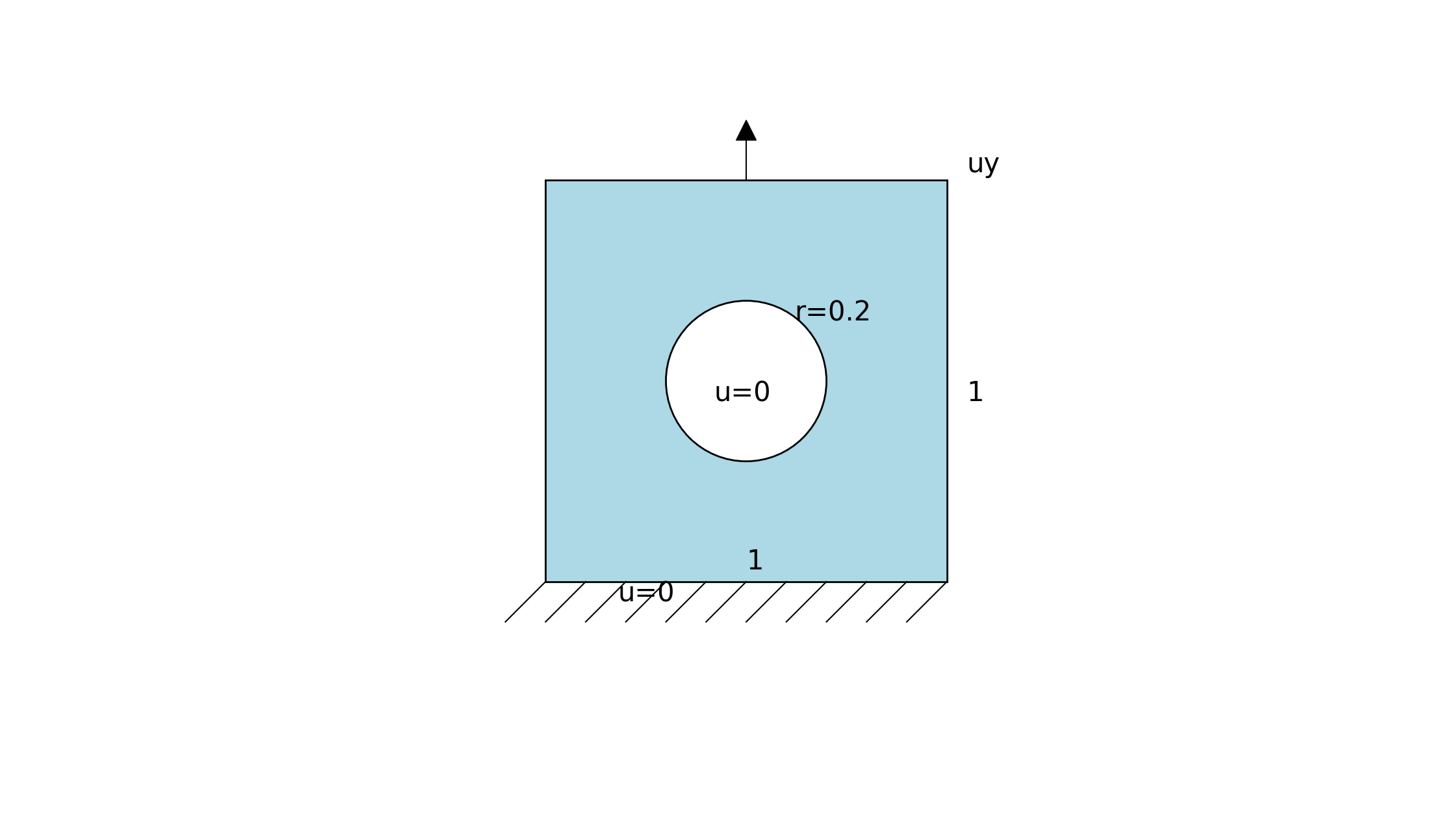
This example examines a rigid circular inclusion within a square plate, subjected to a vertical upward displacement applied to the top surface. The domain is defined as the rectangular region , featuring a circular hole of radius centered at the origin, as depicted in Figure 1. The material properties are specified as follows: a critical energy release rate of , a length scale factor of , Young’s modulus of , and Poisson’s ratio of . The boundary conditions include a Dirichlet boundary condition at the upper boundary (), where the displacement increases by for the first 5 steps and then by for the next 25 steps. Additionally, the displacement is set to zero at the center of the circular notch.
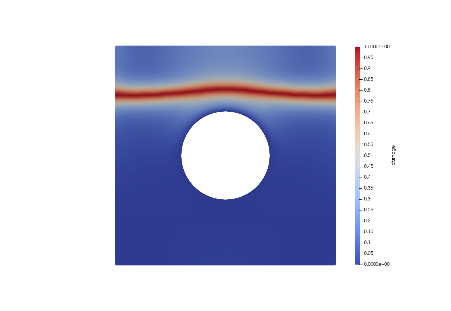
In this example, we investigate the performance and computational efficiency of different finite element methods with varying polynomial degrees () and mesh sizes () for simulating a phase-field fracture model. Figure 2 shows the final fracture morphology of the model.
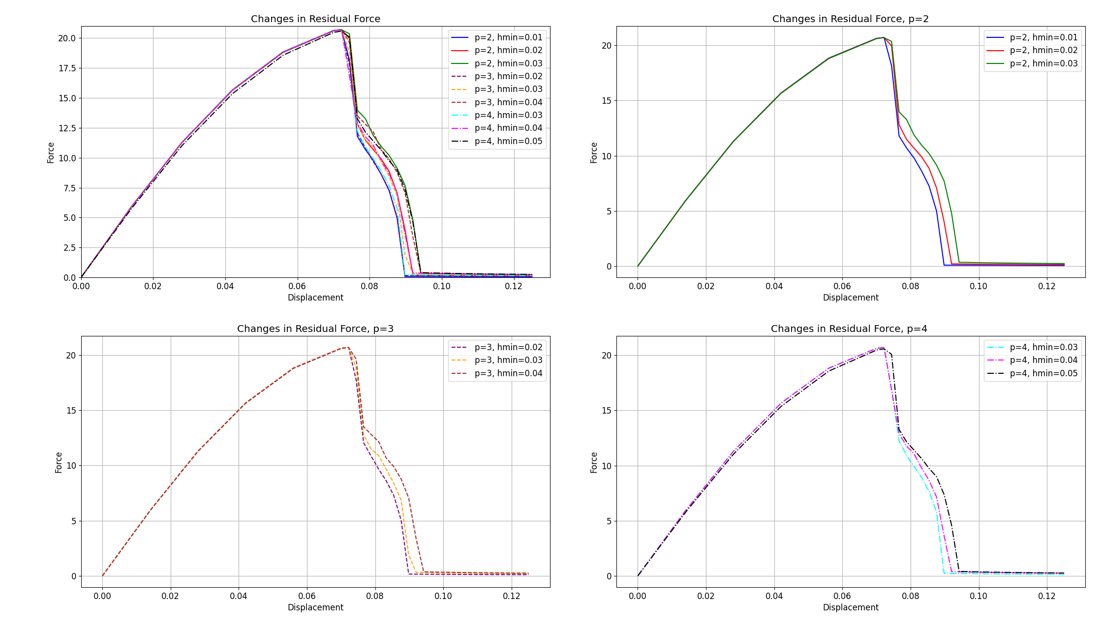
As shown in Figure 2, the residual force curves for different polynomial degrees () and mesh sizes ( to ) reveal significant differences in terms of numerical stability and convergence.
For the lower-order finite element method (), the residual force curves exhibit considerable variability, especially for finer meshes ( to ). During the phase where the residual force rapidly decreases after fracture, these curves show poor convergence, indicating that the lower-order method struggles to provide accurate results without significantly finer mesh sizes. This behavior is particularly evident in the early stages of crack propagation, where the residual force curves for diverge more noticeably compared to higher-order methods. This suggests that the lower-order method is more sensitive to mesh refinement and requires finer meshes to achieve stable and accurate results.
In contrast, the higher-order methods ( and ) demonstrate superior numerical stability and convergence. The residual force curves for these methods nearly coincide across different mesh sizes, indicating that higher-order methods are less sensitive to mesh refinement. Notably, the method shows exceptional consistency across mesh sizes, suggesting that even larger mesh sizes, such as , can still maintain high accuracy and good convergence. This is particularly evident in the post-fracture phase, where the residual force curves for remain tightly clustered, regardless of the mesh size. This behavior highlights the robustness of higher-order methods in handling the complexities of crack propagation, even with coarser meshes.
Higher-order methods ( and ) significantly improve the numerical accuracy and convergence of phase-field fracture simulations, particularly for larger mesh sizes where lower-order methods () struggle to maintain stability. The residual force curves for higher-order methods exhibit remarkable consistency across different mesh sizes, demonstrating their robustness in handling complex crack propagation problems.
5 Summary
In this study, we investigated the numerical simulation of phase-field fracture models using penalty finite element methods of varying orders. Our results demonstrate that higher-order finite element methods (with and ) can achieve high accuracy even with coarser mesh sizes, making them a highly efficient option for modeling fracture behavior in engineering applications. Specifically, the analysis revealed that, for a given mesh size, higher-order methods exhibited superior consistency and convergence properties compared to the lower-order method (), which required finer meshes to achieve similar accuracy.
However, the results were sensitive to mesh refinement. Coarser meshes introduced some numerical errors, especially in higher-order finite element methods. While these errors remained within acceptable bounds for most practical purposes, it is crucial to carefully select mesh sizes to balance computational efficiency and accuracy. By optimizing mesh sizes and element orders, engineers can achieve an optimal trade-off between solution accuracy and computational cost.
Our future work will focus on extending this framework to more complex geometries and dynamic fracture problems, where time-dependent behavior plays a significant role. Additionally, the incorporation of material nonlinearity and adaptive refinement strategies will be explored to further enhance both the accuracy and efficiency of the simulations. These advancements could significantly improve the versatility of the proposed method, enabling its application to a wider range of real-world fracture problems in both engineering and materials science.
References
- Ambati et al. [2014] Ambati, M., Gerasimov, T., De Lorenzis, L., 2014. A review on phase-field models of brittle fracture and a new fast hybrid formulation. Computational Mechanics 55, 383–405. doi:10.1007/s00466-014-1109-y.
- Amiri et al. [2016] Amiri, F., Millán, D., Arroyo, M., Silani, M., Rabczuk, T., 2016. Fourth order phase-field model for local max-ent approximants applied to crack propagation. Computer Methods in Applied Mechanics and Engineering 312, 254–275. doi:https://doi.org/10.1016/j.cma.2016.02.011.
- Arnold [1982] Arnold, D.N., 1982. An interior penalty finite element method with discontinuous elements. SIAM Journal on Numerical Analysis 19, 742–760. URL: https://doi.org/10.1137/0719052, doi:10.1137/0719052.
- Babuška and Zlámal [1973] Babuška, I., Zlámal, M., 1973. Nonconforming elements in the finite element method with penalty. SIAM Journal on Numerical Analysis 10, 863–875. URL: http://www.jstor.org/stable/2156320.
- Borden et al. [2014] Borden, M.J., Hughes, T.J.R., Landis, C.M., Verhoosel, C.V., 2014. A higher-order phase-field model for brittle fracture: Formulation and analysis within the isogeometric analysis framework. Computer Methods in Applied Mechanics and Engineering 273, 100–118. doi:https://doi.org/10.1016/j.cma.2014.01.016.
- Borden et al. [2012] Borden, M.J., Verhoosel, C.V., Scott, M.A., Hughes, T.J., Landis, C.M., 2012. A phase-field description of dynamic brittle fracture. Computer Methods in Applied Mechanics and Engineering 217-220, 77–95. URL: https://www.sciencedirect.com/science/article/pii/S0045782512000199, doi:https://doi.org/10.1016/j.cma.2012.01.008.
- Bourdin et al. [2000] Bourdin, B., Francfort, G., Marigo, J.J., 2000. Numerical experiments in revisited brittle fracture. Journal of the Mechanics and Physics of Solids 48, 797–826. URL: https://www.sciencedirect.com/science/article/pii/S0022509699000289, doi:https://doi.org/10.1016/S0022-5096(99)00028-9.
- Brenner and Sung [2005] Brenner, S.C., Sung, L.Y., 2005. interior penalty methods for fourth order elliptic boundary value problems on polygonal domains. Journal of Scientific Computing 22/23, 83–118. doi:10.1007/s10915-004-4783-1.
- Douglas and Dupont [1976] Douglas, J., Dupont, T., 1976. Interior penalty procedures for elliptic and parabolic galerkin methods, in: Glowinski, R., Lions, J.L. (Eds.), Computing Methods in Applied Sciences. Springer Berlin Heidelberg, Berlin, Heidelberg, pp. 207–216.
- Hughes [2012] Hughes, T.J., 2012. The Finite Element Method: Linear Static and Dynamic Finite Element Analysis. Dover Civil and Mechanical Engineering, Dover Publications. URL: https://books.google.com/books?id=cHH2n_qBK0IC.
- Miehe et al. [2016] Miehe, C., Teichtmeister, S., Aldakheel, F., 2016. Phase-field modelling of ductile fracture: A variational gradient-extended plasticity-damage theory and its micromorphic regularization. Philosophical Transactions of the Royal Society A: Mathematical, Physical and Engineering Sciences 374, 20150170. doi:10.1098/rsta.2015.0170.
- Nguyen et al. [2015] Nguyen, V.P., Anitescu, C., Bordas, S.P., Rabczuk, T., 2015. Isogeometric analysis: An overview and computer implementation aspects. Mathematics and Computers in Simulation 117, 89–116. URL: https://www.sciencedirect.com/science/article/pii/S0378475415001214, doi:https://doi.org/10.1016/j.matcom.2015.05.008.
- Scott and Zhang [1990] Scott, L.R., Zhang, L., 1990. Finite element approximation of higher-order differential equations: The interior penalty method. Mathematics of Computation 54, 381–405. doi:10.1090/S0025-5718-1990-1022412-1.
- Shao et al. [2024] Shao, Y., Duan, Q., Chen, R., 2024. Adaptive meshfree method for fourth-order phase-field model of fracture using consistent integration schemes. Computational Materials Science 233, 112743. doi:https://doi.org/10.1016/j.commatsci.2023.112743.
- Svolos et al. [2022] Svolos, L., Mourad, H.M., Manzini, G., Garikipati, K., 2022. A fourth-order phase-field fracture model: Formulation and numerical solution using a continuous/discontinuous galerkin method. Journal of the Mechanics and Physics of Solids 165, 104910. doi:https://doi.org/10.1016/j.jmps.2022.104910.
- Tanné et al. [2018] Tanné, E., Li, T., Bourdin, B., Marigo, J.J., Maurini, C., 2018. Crack nucleation in variational phase-field models of brittle fracture. Journal of the Mechanics and Physics of Solids 110, 80–99. URL: https://www.sciencedirect.com/science/article/pii/S0022509617306543, doi:https://doi.org/10.1016/j.jmps.2017.09.006.
- Wei et al. [2017–2025] Wei, H., Tian, T., Huang, Y., 2017–2025. Fealpy: Finite element analysis library in python. URL: https://github.com/weihuayi/fealpy.
- Wheeler [1978] Wheeler, M.F., 1978. An elliptic collocation-finite element method with interior penalties. SIAM Journal on Numerical Analysis 15, 152–161. URL: https://doi.org/10.1137/0715010, doi:10.1137/0715010, arXiv:https://doi.org/10.1137/0715010.
- Wu and Cervera [2017] Wu, J.Y., Cervera, M., 2017. Strain localization of elastic-damaging frictional-cohesive materials: Analytical results and numerical verification. Materials 10. URL: https://www.mdpi.com/1996-1944/10/4/434, doi:10.3390/ma10040434.
- Wu et al. [2020a] Wu, J.Y., Huang, Y., Nguyen, V.P., 2020a. On the bfgs monolithic algorithm for the unified phase field damage theory. Computer Methods in Applied Mechanics and Engineering 360, 112704. URL: https://www.sciencedirect.com/science/article/pii/S0045782519305924, doi:https://doi.org/10.1016/j.cma.2019.112704.
- Wu and Nguyen [2018] Wu, J.Y., Nguyen, V.P., 2018. A length scale insensitive phase-field damage model for brittle fracture. Journal of the Mechanics and Physics of Solids 119, 20–42. URL: https://www.sciencedirect.com/science/article/pii/S0022509618302643, doi:https://doi.org/10.1016/j.jmps.2018.06.006.
- Wu et al. [2020b] Wu, J.Y., Nguyen, V.P., Nguyen, C.T., Sutula, D., Sinaie, S., Bordas, S.P., 2020b. Chapter one - phase-field modeling of fracture, Elsevier. volume 53 of Advances in Applied Mechanics, pp. 1–183. URL: https://www.sciencedirect.com/science/article/pii/S0065215619300134, doi:https://doi.org/10.1016/bs.aams.2019.08.001.