A Tale of Two Learning Algorithms:
Multiple Stream Random Walk and Asynchronous Gossip

Abstract

Although gossip and random walk-based learning algorithms are widely known for decentralized learning, there has been limited theoretical and experimental analysis to understand their relative performance for different graph topologies and data heterogeneity. We first design and analyze a random walk-based learning algorithm with multiple streams (walks), which we name asynchronous “Multi-Walk (MW)”. We provide a convergence analysis for MW w.r.t iteration (computation), wall-clock time, and communication. We also present a convergence analysis for “Asynchronous Gossip”, noting the lack of a comprehensive analysis of its convergence, along with the computation and communication overhead, in the literature. Our results show that MW has better convergence in terms of iterations as compared to Asynchronous Gossip in graphs with large diameters (e.g., cycles), while its relative performance, as compared to Asynchronous Gossip, depends on the number of walks and the data heterogeneity in graphs with small diameters (e.g., complete graphs). In wall-clock time analysis, we observe a linear speed-up with the number of walks and nodes in MW and Asynchronous Gossip, respectively. Finally, we show that MW outperforms Asynchronous Gossip in communication overhead, except in small-diameter topologies with extreme data heterogeneity. These results highlight the effectiveness of each algorithm in different graph topologies and data heterogeneity. Our codes are available for reproducibility.

1 Introduction

Decentralized learning has gained significant attention as a robust alternative to traditional centralized approaches, addressing critical limitations such as communication bottlenecks and single points of failure (Tsitsiklis, 1984; Nedić & Ozdaglar, 2009; McMahan et al., 2023). Among decentralized methods, two prominent approaches have emerged: gossip and random walk-based algorithms. While both paradigms have been extensively studied (Boyd et al., 2006; Lian et al., 2017; Koloskova et al., 2019; Bertsekas, 1997; Ayache & Rouayheb, 2020; Sun et al., 2018; Needell et al., 2015), a gap remains in understanding their relative performance and trade-offs across different graph topologies and data heterogeneity. Specifically, a comprehensive analysis comparing their convergence rates, communication, and computational overhead is still lacking, which constitutes the primary focus of this work.

Gossip algorithms advocate that nodes in a graph iteratively update their models with Stochastic Gradient Descent (SGD) (Robbins, 1951; Bottou et al., 2018) and exchange the updated models with their neighbors, leading to global consensus over time. Gossip can employ synchronous communication (Lian et al., 2017; Koloskova et al., 2020), where nodes must wait for all nodes to update their model in each round. However, in the presence of straggler nodes or nodes with varying computation speeds (Kairouz et al., 2021), synchronous gossip results in significant idle times for fast nodes and creates bottlenecks (Chen et al., 2017). Asynchronous gossip algorithms (Baudet, 1978; Tsitsiklis et al., 1984; Recht et al., 2011) have been developed to leverage available nodes more effectively, allowing nodes to compute gradients using a stale model and communicate in a decentralized manner, thereby eliminating the need to wait for all nodes (Lian et al., 2018; Nabli et al., 2023; Nadiradze et al., 2022; Bornstein et al., 2022; Even et al., 2024). In both synchronous and asynchronous cases, gossip incurs high communication costs due to frequent message exchange among nodes.

The random walk-based learning algorithms suggest that one node at a time updates a model with its local data. The node then randomly selects a neighbor and sends the updated model to it. This neighbor becomes the next activated node and updates the model using its own local data. This process repeats until convergence. However, random walk-based algorithms (Ayache & Rouayheb, 2020; Sun et al., 2018; Needell et al., 2015) are single stream, i.e., only one node updates the model at any given time, which leads to slow convergence. Multiple streams can be used to improve the convergence time, but the coordination and interaction of multiple streams is an unexplored area in the random walk-based learning literature.

To understand the relative performance of gossip and random walk-based learning for different graph topologies and data heterogeneity, we first design and analyze a random walk-based learning algorithm with multiple streams, which we name asynchronous “Multi-Walk (MW)”. Then, we provide a comprehensive analysis of both MW and Asynchronous Gossip w.r.t iteration (computation), wall-clock time, and communication. Our main contributions are as follows:

Design of MW algorithm. We design a random walk-based learning algorithm with multiple streams, Multi-Walk (MW). The core idea behind MW is to improve the convergence rate of random walk-based methods by initiating multiple random walks (streams) simultaneously across the graph. This strategy increases the number of concurrent computations, enabling the algorithm to improve its convergence rate. MW allows for a trade-off between convergence speed and resource utilization by adjusting the number of walks. There is no need for special coordination among the walks, as each walk operates independently on the graph. Furthermore, we demonstrate that the algorithm achieves a linear speedup with the number of walks.

Comprehensive analysis of MW and Asynchronous Gossip. We provide an in-depth examination of both Asynchronous Gossip and our proposed MW algorithms. Specifically, we analyze their convergence properties w.r.t iterations (computation), wall-clock time, and communication overhead. This detailed comparison addresses a significant gap in the literature, offering insights into the performance trade-offs of these methods. We analyze both algorithms under the assumption of non-convex, smooth, and heterogeneous loss functions, without any upper bounds on computation or communication delays.

Theoretical insights. Our analysis demonstrates that MW exhibits superior performance on graphs with larger diameters, while Asynchronous Gossip is likely a better choice for small-diameter graphs in terms of iteration complexity. Specifically, MW outperforms Asynchronous Gossip in both iteration complexity and communication overhead on network topologies such as cycles. We showed that in iid setting, on graphs where $p=\mathcal{O}\left(\frac{1}{V}\right),$ with $V$ representing the number of nodes in the network, MW shows superior performance compared to Asynchronous Gossip. Here, $p$ refers to the spectral gap of $\mathbf{P}^{\top}\mathbf{P}$, where $\mathbf{P}$ is the mixing matrix of Asynchronous Gossip. Intuitively, $p^{-1/2}$ correlates with the graph’s diameter. When evaluating convergence in terms of clock time, Asynchronous Gossip benefits from a linear speed-up with the number of nodes. MW outperforms Asynchronous Gossip when considering convergence in terms of communication overhead except in small-diameter with extreme data heterogeneity (non-iid) settings. This highlights the effectiveness of each algorithm in different scenarios.

Empirical validation. We conduct experiments to validate our theoretical findings. The results confirm that MW converges faster w.r.t iterations for graphs with larger diameters, such as cycles. However, this advantage does not hold for topologies with smaller diameters, such as complete graphs. We also examine the impact of non-iid data in an Erdős–Rényi topology, observing behavior consistent with the predictions of our theorem. To highlight the benefits of MW over Asynchronous Gossip in communication-constrained settings, we conducted experiments measuring convergence rates w.r.t total transmitted bits during the fine-tuning of OPT-$125$M (Zhang et al., 2022) as a large language model. Overall, the experiments provide valuable insights into the performance trade-offs between gossip and random walk-based decentralized learning algorithms.

2 Related Work

Decentralized optimization algorithms have been extensively explored in the literature, where nodes in a graph collaborate with their neighbors to solve optimization problems (Tsitsiklis, 1984; Nedić & Ozdaglar, 2009; Duchi et al., 2012; Yuan et al., 2015; Gholami & Seferoglu, 2024). These algorithms mostly rely on mixing information among nodes, leading to a considerable communication overhead. Decentralized algorithms based on Gossip involve a mixing step where nodes compute their new models by mixing their own and neighbors’ models (Xiao & Boyd, 2003; Lian et al., 2017; Koloskova et al., 2020). Model updates propagate gradually over the graph due to iterative gossip averaging. However, this is costly in terms of communication as it requires $\mathcal{O}(|\mathcal{E}|)$ data exchange per model update for a graph with an edge set of $\mathcal{E}$, where $|\cdot|$ is the size of a set.

The study of asynchronous optimization has its roots in earlier works such as those by Baudet (1978), with one of the first convergence results for Asynchronous SGD provided by Tsitsiklis (1984). Many works have focused on asynchronous algorithms in federated learning settings (Agarwal & Duchi, 2011; Lian et al., 2015; Zheng et al., 2016; Feyzmahdavian & Johansson, 2021; Mishchenko et al., 2022; Koloskova et al., 2022). Going to decentralized setting along with asynchrony, Assran & Rabbat (2021) addresses asymmetric asynchronous communication (push-sum), but to guarantee convergence, their approach requires all nodes to participate in computations synchronously at each iteration. Nadiradze et al. (2022) explores quantized gossip communication; however, their work does not account for delays in communication or computation. (Bornstein et al., 2022) proposes a wait-free decentralized algorithm that allows nodes to have different computation speeds, but they do not consider any communication delays. Nabli et al. (2023) considers a framework for communication acceleration on time-varying topologies with local stochastic gradient steps. However, they do not consider computation or communication delays. The two closest works to ours are Lian et al. (2018) and Even et al. (2024). The former introduced the Asynchronous Decentralized Stochastic Gradient Descent algorithm (AD-PSGD), one of the most prominent asynchronous decentralized methods. In this paper, we consider the same algorithm as Asynchronous Gossip and further analyze it to understand its relative performance as compared to MW. Unlike our analysis, Lian et al. (2018) derive a convergence rate under the assumption of an upper bound on computation delays, and their result is valid only when the number of iterations exceeds a certain threshold. Even et al. (2024) introduces the Asynchronous SGD on Graph (AGRAF SGD) algorithm, which operates with a continuous while true loop for communication among nodes without any assumptions about the frequency and amount of communication. This design makes it theoretically infeasible to quantify the communication overhead.

On the other end of the spectrum of decentralized learning algorithms are random walk-based approaches (Ayache & Rouayheb, 2020). When there is only a single walk in the graph, the problem closely resembles to data sampling for stochastic gradient descent, e.g., Sun et al. (2018); Needell et al. (2015), and the distinction between synchronous and asynchronous operations becomes irrelevant. We extend this concept by developing MW as a generalized version in which multiple walks operate on a graph in an asynchronous manner.

3 Setup and Algorithm Design

Figure 1: Example instance of MW in a $3$-node network with two walks ($R=2$), where $t$ represents the iteration number.

We model the underlying network topology with a connected graph $G=(\mathcal{V},\mathcal{E})$, where $\mathcal{V}$ is the set of vertices (nodes) and $\mathcal{E}$ is the set edges. The vertex set contains $V$ nodes, i.e., $|\mathcal{V}|=V$. If node $i$ is connected to node $j$ through a communication link, then $\{i,j\}$ is in the edge set, i.e., $\{i,j\}\in\mathcal{E}$. The set of the nodes that node $i$ is connected to and can transmit data is called the neighbors of node $i$, and the neighbor set of node $i$ is denoted by $\mathcal{N}_{i}$.

Assume that the nodes in the network jointly minimize a $d$-dimensional function $f:\mathbb{R}^{d}\rightarrow\mathbb{R}$. The goal is to solve optimization problems where the elements of the objective function (i.e., the data used in machine learning tasks) are distributed across different nodes,

$$\min_{\mathbf{x}\in\mathbb{R}^{d}}\left[f(\mathbf{x}):=\frac{1}{V}\sum_{v\in\mathcal{V}}\left[f_{v}(\mathbf{x})=\operatorname{\mathbb{E}}_{\xi\sim\mathcal{D}_{v}}F_{v}(\mathbf{x},\xi)\right]\right].$$ (1)

$F_{v}(\mathbf{x},\xi):\mathbb{R}^{d}\rightarrow\mathbb{R}$ is the loss function of $\mathbf{x}$ associated with data sample $\xi$ at node $v$. The loss function on local dataset $\mathcal{D}_{v}$ at node $v$ is $f_{v}(\mathbf{x})$.

3.1 Asynchronous Multi-Walk (MW) Algorithm

This section presents our novel multi-walk (MW) algorithm. MW considers the standard asynchronous SGD for model updates. To achieve consensus, communication is performed using multiple walks. MW algorithm is summarized in Algorithm 1, and detailed in the following.

Algorithm 1 Asynchronous MW with $R$ walks

1:Start walk $r$ at node $r-1$, which sets $\mathbf{x}^{r}_{0}=\mathbf{x}_{0}$, where $r\in\{1,\dots,R\}$.

2:Node $0$ initializes $\{u^{r}\}_{r\in\{1,\dots,R\}}$ with $\mathbf{x}_{0}$.

3:Set $l=1$, which is the last walk that visited Node $0$.

4:for $t=0$ to $T-1$ do

5:  if Node $v_{t}$ finishes the calculation of $\nabla F_{v_{t}}(\mathbf{x}^{r_{t}}_{t-\tau_{t}},\xi_{t})$ at point $\mathbf{x}^{r_{t}}_{t-\tau_{t}}$, which began transmission to node $v_{t}$ by one of its neighbors at $t-\tau_{t}$ via walk $r_{t}$ then iteration $t$ is triggered. Node $v_{t}$ executes lines 6-12.

6:   $\mathbf{x}^{r_{t}}_{t+1}=\mathbf{x}^{r_{t}}_{t-\tau_{t}}-\eta_{t}\nabla F_{v_{t}}(\mathbf{x}^{r_{t}}_{t-\tau_{t}},\xi_{t})$

7:   if $v_{t}=0$ then

8:     $\mathbf{x}^{r_{t}}_{t+1}=u^{l}+\frac{1}{R}(\mathbf{x}^{r_{t}}_{t+1}-u^{r_{t}})$.

9:     $u^{r_{t}}=\mathbf{x}^{r_{t}}_{t+1}$.

10:     $l=r_{t}$.    

11:   Choose the next node based matrix $\mathbf{P}$.

12:   Send $\mathbf{x}^{r_{t}}_{t+1}$ to the next node via walk $r_{t}$.   

First, we assume that there are $R$ walks over the graph. Without loss of generality, we start the walk $r$ at node $r-1$ by setting $\mathbf{x}^{r}_{0}=\mathbf{x}_{0}$, where $r\in\{1,\dots,R\}$. These initial nodes start computing the stochastic gradient at $\mathbf{x}_{0}$ using their local data. In order to mix the information among walks, we need to have a dedicated node that we assume to be Node $0$ without loss of generality. We also define $\{u^{r}\}_{r\in\{1,\dots,R\}}$ where $u^{r}$ is a copy of walk $r$’s model at the most recent instance when that walk was at Node $0$. At Node $0$, we initialize $\{u^{r}\}_{r\in\{1,\dots,R\}}$ with $\mathbf{x}_{0}$ that will be used in the mixing. Assume that $l$ is the last walk that visited node Node $0$, which is initialized with $1$. Throughout the algorithm, each node receiving a model via a walk computes its gradient at its own pace, using its local data and the received model. On line 5, once a node (denoted as $v_{t}$) completes computing the gradient using the model received via walk $r_{t}$, iteration $t$ is triggered. We note that only one gradient computation completion event happens in each iteration. On line 6, node $v_{t}$ incorporates the computed gradient to update the model using the step size $\eta_{t}$. Note that communicating the model of walk $r_{t}$ to node $v_{t}$ and computing the gradient takes $\tau_{t}$ iterations. Now, if $v_{t}$ is Node $0$, we need to mix the current walk, $r_{t}$, with other walks. This is done in lines 8–10. On line 8, we incorporate the newly introduced updates of walk $r_{t}$, i.e., $(\mathbf{x}^{r_{t}}_{t+1}-u^{r_{t}})$, which have not been mixed before, into the latest model ($u^{l}$) with a weight of $\frac{1}{R}$. We update the last applied model of walk $r_{t}$ ($u^{r_{t}}$) and the latest walk ($l$) on lines 9 and 10. Finally, node $v_{t}$ chooses the next node based on the transition matrix $\mathbf{P}$ and sends the model. We note that $\mathbf{P}$ is the transition matrix of a Markov chain, representing each walk, where $p_{ij}$ in row $i$ and column $j$ of $\mathbf{P}$ denotes the probability of choosing the next node as $j$ given that the current node is $i$. Figure 1 illustrates the operation of MW with two walks in a $3$-node network.

3.2 Asynchronous Gossip Algorithm

This section presents the Asynchronous Gossip algorithm based on Lian et al. (2018). During the course of the algorithm, all nodes are engaged in gradient computations. At iteration $t$, node $v_{t}$ is selected randomly among all the nodes. When node $v_{t}$ finishes computing the gradient at point $\mathbf{x}^{v_{t}}_{t-\tau_{t}}$, i.e., $\nabla F_{v_{t}}(\mathbf{x}^{v_{t}}_{t-\tau_{t}},\xi_{t})$, iteration $t$ is triggered (line 4). The gradient is computed with a delay $\tau_{t}$ and subsequently applied to the current model of node $v_{t}$, i.e., $\mathbf{x}^{v_{t}}_{t}$, using learning rate $\eta_{t}$ (line 5). At the end of each iteration, a gossip averaging step is performed based on mixing matrix $\mathbf{P}$ (line 6), where $p_{ij}$, which is the element of $\mathbf{P}$, is the weight of node $j$’s model in the weighted averaging used to find node $i$’s new model. After gossip averaging is finished, node $v_{t}$ starts computing gradient at point $\mathbf{x}^{v_{t}}_{t+1}$ (line 7).

Algorithm 2 Asynchronous Gossip (AD-PSGD)

1:Initialize local models $\mathbf{x}^{v}_{t}=\mathbf{x}_{0}$ in all nodes. All nodes start computing the stochastic gradient.

2:for $t=0$ to $T-1$ do

3:  Node $v_{t}$ is randomly sampled from all nodes.

4:  if Node $v_{t}$ finishes computing the gradient at point $\mathbf{x}^{v_{t}}_{t-\tau_{t}}$, i.e., $\nabla F_{v_{t}}(\mathbf{x}^{v_{t}}_{t-\tau_{t}},\xi_{t})$ then iteration $t$ is triggered. Node $v_{t}$ executes lines 5-7.

5:   $\mathbf{x}^{v_{t}}_{t+\frac{1}{2}}=\mathbf{x}^{v_{t}}_{t}-\eta_{t}\nabla F_{v_{t}}(\mathbf{x}^{v_{t}}_{t-\tau_{t}},\xi_{t})$.

6:   $\mathbf{x}^{v}_{t+1}=\sum_{i\in\mathcal{N}_{v}}p_{vi}\mathbf{x}^{i}_{t+\frac{1}{2}}$ (gossip averaging for all $v\in\mathcal{V}$ based on mixing matrix $\mathbf{P}$)

7:   Start computing gradient at point $\mathbf{x}^{v_{t}}_{t+1}$.   

Table 1: Comparison of the convergence rate and communication overhead in iid setting for Metropolis-Hastings $\mathbf{P}$.

Topology	MW		Asynchronous Gossip
	Convergence rate	Comm-cost	Convergence rate	Comm-cost
cycle ($p=\Theta(\frac{1}{V^{2}})$)	${\mathcal{O}\bigg{(}\frac{\sigma}{\sqrt{T}}+(\frac{R\sqrt{V\sigma^{2}}}{T})^{\frac{2}{3}}\bigg{)}}$✓	${\Theta(T)}$	$\mathcal{O}\bigg{(}\frac{\sigma}{\sqrt{T}}+(\frac{V\sqrt{V^{2}\sigma^{2}}}{T})^{\frac{2}{3}}\bigg{)}$	$\Theta(VT)$
2d-torus ($p=\Theta(\frac{1}{V})$)	${\mathcal{O}\bigg{(}\frac{\sigma}{\sqrt{T}}+(\frac{R\sqrt{V\sigma^{2}}}{T})^{\frac{2}{3}}\bigg{)}}$✓	${\Theta(T)}$	${\mathcal{O}\bigg{(}\frac{\sigma}{\sqrt{T}}+(\frac{V\sqrt{V\sigma^{2}}}{T})^{\frac{2}{3}}\bigg{)}}$	$\Theta(VT)$
complete ($p=1$)	$\mathcal{O}\bigg{(}\frac{\sigma}{\sqrt{T}}+(\frac{R\sqrt{V\sigma^{2}}}{T})^{\frac{2}{3}}\bigg{)}$[✓if $R\leq\sqrt{V}$]	${\Theta(T)}$	${\mathcal{O}\bigg{(}\frac{\sigma}{\sqrt{T}}+(\frac{V\sqrt{\sigma^{2}}}{T})^{\frac{2}{3}}\bigg{)}}$[✓if $R\geq\sqrt{V}$]	$\Theta(V^{2}T)$

Table 2: Comparison of the convergence rate and communication overhead in noniiid setting for Metropolis-Hastings $\mathbf{P}$.

Topology	MW		Asynchronous Gossip
	Convergence rate	Comm-cost	Convergence rate	Comm-cost
cycle ($p=\Theta(\frac{1}{V^{2}})$)	${\mathcal{O}\bigg{(}\sqrt{\frac{\sigma^{2}+\zeta^{2}}{T}}+(\frac{R\sqrt{V\sigma^{2}+V^{3}\zeta^{2}}}{T})^{\frac{2}{3}}\bigg{)}}$✓	${\Theta(T)}$	$\mathcal{O}\bigg{(}\sqrt{\frac{\sigma^{2}+\zeta^{2}}{T}}+(\frac{V\sqrt{V^{2}\sigma^{2}+V^{4}\zeta^{2}}}{T})^{\frac{2}{3}}\bigg{)}$	$\Theta(VT)$
2d-torus ($p=\Theta(\frac{1}{V})$)	${\mathcal{O}\bigg{(}\sqrt{\frac{\sigma^{2}+\zeta^{2}}{T}}+(\frac{R\sqrt{V\sigma^{2}+H^{2}\zeta^{2}}}{T})^{\frac{2}{3}}\bigg{)}}$	${\Theta(T)}$	${\mathcal{O}\bigg{(}\sqrt{\frac{\sigma^{2}+\zeta^{2}}{T}}+(\frac{V\sqrt{V\sigma^{2}+V^{2}\zeta^{2}}}{T})^{\frac{2}{3}}\bigg{)}}$	$\Theta(VT)$
complete ($p=1$)	${\mathcal{O}\bigg{(}\sqrt{\frac{\sigma^{2}+\zeta^{2}}{T}}+(\frac{R\sqrt{V\sigma^{2}+V^{2}\zeta^{2}}}{T})^{\frac{2}{3}}\bigg{)}}$	${\Theta(T)}$	${\mathcal{O}\bigg{(}\sqrt{\frac{\sigma^{2}+\zeta^{2}}{T}}+(\frac{V\sqrt{\sigma^{2}+\zeta^{2}}}{T})^{\frac{2}{3}}\bigg{)}}$	$\Theta(V^{2}T)$

4 Convergence Analysis

We use the following standard assumptions in our analysis.

1. Smooth local loss. $f_{v}(\mathbf{x})$ is differentiable and its gradient is $L$-Lipschitz for $v\in\mathcal{V}$, i.e., $\|\nabla f_{v}(\mathbf{y})-\nabla f_{v}(\mathbf{x})\|\leq~L\|\mathbf{y}-\mathbf{x}\|,\quad\forall\mathbf{x},\mathbf{y}\in\mathbb{R}^{d}$.

2. Bounded local variance. The variance of the stochastic gradient is bounded for $v\in\mathcal{V}$, i.e., $\operatorname{\mathbb{E}}_{\xi\sim\mathcal{D}_{v}}\|\nabla F_{v}(\mathbf{x},\xi)-\nabla f_{v}(\mathbf{x})\|^{2}\leq\sigma^{2}$.

3. Bounded diversity. The diversity of the local loss functions are bounded for $v\in\mathcal{V}$, i.e., $\|\nabla f_{v}(\mathbf{x})-\nabla f(\mathbf{x})\|^{2}\leq~\zeta^{2}$.

4. Transition (mixing) matrix. In Algorithm 1, $\mathbf{P}$ is the transition matrix of an irreducible and aperiodic Markov chain, representing each walk. In Algorithm 2, it defines the mixing step of the gossip averaging. Matrix $\mathbf{P}$ is doubly stochastic ($\mathbf{P}\mathbf{1}=\mathbf{1}$, $\mathbf{1}^{\top}\mathbf{P}=\mathbf{1}^{\top}$) and the spectral gaps of $\mathbf{P}^{\top}\mathbf{P}$ and $\mathbf{P}$ are denoted by $p$ and $p^{\prime}$, respectively.

4.1 Convergence rate w.r.t iterations

Theorem 4.1.

Multi-Walk (MW). Let assumptions 1-4 hold, with a constant and small enough learning rate $\eta$ (potentially depending on $T$), after $T$ iterations of Algorithm 1, $\frac{1}{T}\sum_{t=0}^{T-1}\operatorname{\mathbb{E}}\|\nabla f(\mathbf{x}^{r_{t}}_{t})\|^{2}$ is

$$\mathcal{O}\bigg{(}\hskip-3.0pt\frac{FLRH}{T}\hskip-2.0pt+\hskip-2.0pt\frac{R\zeta^{2}}{p^{\prime}T}\hskip-2.0pt+\hskip-2.0pt\sqrt{\frac{\hskip-2.0ptFL\hskip-2.0pt\left(\sigma^{2}\hskip-2.0pt+\hskip-2.0pt\zeta^{2}\right)}{T}}\hskip-2.0pt+\hskip-2.0pt(\hskip-1.0pt\frac{FLR\sqrt{V\sigma^{2}+H^{2}\zeta^{2}}}{T}\hskip-2.0pt)\hskip-1.0pt^{\frac{2}{3}}\hskip-2.0pt\bigg{)},$$ (2)

where $F:=f(\mathbf{x}_{0})-f^{*}$, and $H^{2}$ is the second moment of the first return time to Node $0$ for the Markov chain representing each walk. $\Box$

Theorem 4.2.

Asynchronous Gossip. Let assumptions 1-4 hold, with a constant and small enough learning rate $\eta$ (potentially depending on $T$), after $T$ iterations of Algorithm 2, $\frac{1}{T}\sum_{t=0}^{T-1}\operatorname{\mathbb{E}}\|\nabla f(\mathbf{x}^{v_{t}}_{t})\|^{2}$ is

$$\mathcal{O}\bigg{(}\frac{FLV}{pT}+\sqrt{\frac{FL\left(\sigma^{2}+\zeta^{2}\right)}{T}}+(\frac{FLV\sqrt{\frac{\sigma^{2}}{p}+\frac{\zeta^{2}}{p^{2}}}}{T})^{\frac{2}{3}}\bigg{)},$$ (3)

where $F:=f(\mathbf{x}_{0})-f^{*}$. $\Box$

Dominant terms. The dominant term in both (2) and (3) is identically given by $\sqrt{\frac{FL\left(\sigma^{2}+\zeta^{2}\right)}{T}}$. Focusing on the next most significant term for comparison, in (2), this term is given by $(\frac{FLR\sqrt{V\sigma^{2}+H^{2}\zeta^{2}}}{T})^{\frac{2}{3}}$, whereas in (3), it is $(\frac{FLV\sqrt{\frac{\sigma^{2}}{p}+\frac{\zeta^{2}}{p^{2}}}}{T})^{\frac{2}{3}}$. Note that (2) includes a non-dominating term that describes the rate at which walks converge to their steady state. This term is related to the spectral gap of $\mathbf{P}$, represented by $p^{\prime}$. In the following, we compare the dominant terms in the convergence rates of both algorithms in different settings.

Homogeneous data distribution. In iid setting ($\zeta=0$), the differentiating factor in the second dominant term of convergence rate is $\frac{V}{\sqrt{p}}$ for Asynchronous Gossip and $R\sqrt{V}$ for MW. Specifically, for graphs with $p=\mathcal{O}(\frac{V}{R^{2}})$, MW outperforms, while for $p=\Omega(\frac{V}{R^{2}})$, Asynchronous Gossip converges faster w.r.t iterations. It is interesting to observe that the graph’s topology does not impact the performance of MW in iid setting, and the only factors are the number of nodes and walks. We compare convergence rate and communication overhead for each algorithm in Table 1 across three different graph topologies, using the commonly employed Metropolis-Hastings matrix, $\mathbf{P}$, where $p_{ij}=p_{ji}=\min\left\{\frac{1}{\operatorname{deg}(i)+1},\frac{1}{\operatorname{deg}(j)+1}\right\},\quad\text{for }\{i,j\}\in\mathcal{E}.$ Note that computation overhead is the same for both as it is the number of iterations, i.e., $T$, and we do not include that in the table. We observe that for both cycle and $2$D-torus topologies, MW outperforms Asynchronous Gossip in convergence rate. However, when the graph diameter decreases (i.e., $p$ increases), such as in the case of a complete graph, MW loses its advantage. It is important to note that MW consistently requires less communication overhead. In each iteration, MW uses at most one communication, whereas Asynchronous Gossip activates multiple edges for mixing based on the graph topology.

Heterogeneous Data Distribution. In non-iid setting, $\zeta^{2}$ is multiplied by $H^{2}$ for MW and by $p^{2}$ for Asynchronous Gossip. We derived $H^{2}$ for cycle and complete topologies with Metropolis-Hastings transition matrix in Appendix D, and the comparison is summarized in Table 2. We observe that for the cycle topology, MW converges faster w.r.t iterations. However, this advantage diminishes as we move to topologies with smaller diameters. In complete topology, we observe that $\zeta^{2}$ is multiplied by $V^{2}$ in MW, whereas it is multiplied by $1$ in Asynchronous Gossip. This indicates that, as we transition to increasingly non-iid settings in small-diameter topologies, MW perform poorly.

Table 3: Analysis in total transmitted bits ($B$).

Algorithm	Convergence rate	Comp-cost
MW	$\mathcal{O}\bigg{(}\frac{FLRHm}{B}+\frac{R\zeta^{2}m}{p^{\prime}B}+\sqrt{\frac{FLm\left(\sigma^{2}+\zeta^{2}\right)}{B}}+(\frac{FLRm\sqrt{V\sigma^{2}+H^{2}\zeta^{2}}}{B})^{\frac{2}{3}}\bigg{)}$	$\Theta(\frac{B}{m})$
Asynchronous Gossip	$\mathcal{O}\bigg{(}\frac{FLVm\|\mathbf{P}\|_{0}}{pB}+\sqrt{\frac{FLm\|\mathbf{P}\|_{0}\left(\sigma^{2}+\zeta^{2}\right)}{B}}+(\frac{FLVm\|\mathbf{P}\|_{0}\sqrt{\frac{\sigma^{2}}{p}+\frac{\zeta^{2}}{p^{2}}}}{B})^{\frac{2}{3}}\bigg{)}$	$\Theta(\frac{B}{m\|\mathbf{P}\|_{0}})$

Table 4: Analysis in wall-clock time ($Z$).

Algorithm	Convergence rate	Comm-cost	Comp-cost
MW	$\mathcal{O}\bigg{(}\frac{FLHd}{Z}+\frac{\zeta^{2}d}{p^{\prime}Z}+\sqrt{\frac{FLd\left(\sigma^{2}+\zeta^{2}\right)}{RZ}}+(\frac{FLd\sqrt{\sigma^{2}V+\zeta^{2}H^{2}}}{Z})^{\frac{2}{3}}\bigg{)}$	${\Theta(\frac{ZRm}{d})}$	$\Theta(\frac{ZR}{d})$
Asynchronous Gossip	$\mathcal{O}\bigg{(}\frac{FLd}{pZ}+\sqrt{\frac{FLd\left(\sigma^{2}+\zeta^{2}\right)}{VZ}}+(\frac{FLd\sqrt{\frac{\sigma^{2}}{p}+\frac{\zeta^{2}}{p^{2}}}}{Z})^{\frac{2}{3}}\bigg{)}$	$\Theta(\frac{ZVm\|\mathbf{P}\|_{0}}{d})$	$\Theta(\frac{ZV}{d})$

4.2 Convergence rate w.r.t transmitted bits

Assume the model size is $m$ bits. Each iteration of Algorithm 1 and 2 communicates one and $\|\mathbf{P}\|_{0}$ models, respectively. $\|\mathbf{P}\|_{0}$ denote the number of non-zero elements of mixing matrix $\mathbf{P}$.

Corollary 4.3.

Under the condition of Theorem 4.1, 4.2, we get the convergence rate of Algorithm 1, and 2 as shown in Table 3 where $B$ represents total transmitted bits.

The dominating term here is $\sqrt{\frac{FLm\left(\sigma^{2}+\zeta^{2}\right)}{B}}$ for MW and $\sqrt{\frac{FLm\|\mathbf{P}\|_{0}\left(\sigma^{2}+\zeta^{2}\right)}{B}}$ for Asynchronous Gossip. Thus, we observe that in terms of transmitted bits, MW outperforms Asynchronous Gossip if the second dominating term is not considerably large (extreme non-iid setting). Intuitively, in every model transmission, MW executes approximately one computation per model transmission, while Asynchronous Gossip performs $\|\mathbf{P}\|_{0}$ model transmissions per computation. Therefore, MW is a better choice when there is a restriction on the amount of communicated bits.

4.3 Convergence rate w.r.t wall-clock time

In Algorithm 1, assume each walk performs one iteration (computation and communication) with a rate-$\frac{1}{d}$ exponential random variable, independent across walks and over time. The value of $d$ is determined by the average computation and communication delay in the network. Thus, each walk does one iteration in Algorithm 1 according to a rate-$\frac{1}{d}$ Poisson process. Equivalently, this corresponds to all iterations in Algorithm 1 are according to a rate-$\frac{R}{d}$ Poisson process at times $\{Z_{t}\}_{t=0}^{T-1}$ where $\{Z_{t}-Z_{t-1}\}_{t=1}^{T-1}$, denoting the $t$-th iteration duration, are i.i.d. exponentials of rate $\frac{R}{d}$. Therefore, we have $\operatorname{\mathbb{E}}\left[Z_{t}\right]=\frac{td}{R}$ and for any $\delta>0$:

$$Pr\left(|Z_{t}-\frac{td}{R}|\geq\frac{\delta td}{R}\right)\leq 2\exp\left(\frac{-\delta^{2}t}{2}\right).$$ (4)

(4) follows directly from Cramer’s theorem (Boyd et al., 2006). Hence, by multiplying the terms obtained regarding iterations by $\frac{d}{R}$, we obtain the corresponding terms in real time. In other words, the convergence rate in Theorem 4.1 can be transformed to real time ($Z$) by substituting $T$ with $\frac{RZ}{d}$.

For Algorithm 2, we assume each node has a clock that ticks at the times of a rate-$\frac{1}{d}$ Poisson process. Here, the value of $d$ is determined by the average computation and gossip communication delay for nodes. And the same result of (4) is valid by replacing $R$ with $V$.

Corollary 4.4.

Under the condition of Theorem 4.1, 4.2, we get the convergence rate of Algorithms 1 and 2 as shown in Table 4 where $Z$ represents wall-clock time.

The dominating term here is $\sqrt{\frac{FLd\left(\sigma^{2}+\zeta^{2}\right)}{RZ}}$ for MW and $\sqrt{\frac{FLd\left(\sigma^{2}+\zeta^{2}\right)}{VZ}}$ for Asynchronous Gossip. This highlights the advantage of Asynchronous Gossip when considering real-time performance. The reason is that all nodes operate simultaneously, enabling multiple iterations to be completed in a shorter period of time in terms of wall-clock duration. We also observe that MW achieves a linear speed-up proportional to the number of walks, making it competitive with Asynchronous Gossip w.r.t wall-clock time. Increasing the number of walks reduces the impact of the dominant term. If we consider the second dominant term, given by $(\frac{FLd\sqrt{\sigma^{2}V+\zeta^{2}H^{2}}}{Z})^{\frac{2}{3}}$ for MW and $(\frac{FLd\sqrt{\sigma^{2}/p+\zeta^{2}/p^{2}}}{Z})^{\frac{2}{3}}$ for Asynchronous Gossip, we observe that this term favors MW for topologies with large diameters. Here, we also observe that the computation and communication cost of Asynchronous Gossip is higher than that of MW in real time. The communication overhead for Asynchronous Gossip is proportional to $V\|\mathbf{P}\|_{0}$ because all nodes are active, and gossip is used for information dissemination. In contrast, for MW, it is proportional to $R$, as there are $R$ active walks, each performing one peer-to-peer communication. The computation overhead is proportional to $R$ and $V$ in MW and Asynchronous Gossip, respectively, as MW and Asynchronous Gossip have $R$ and $V$ active nodes calculating gradients.

5 Experiments

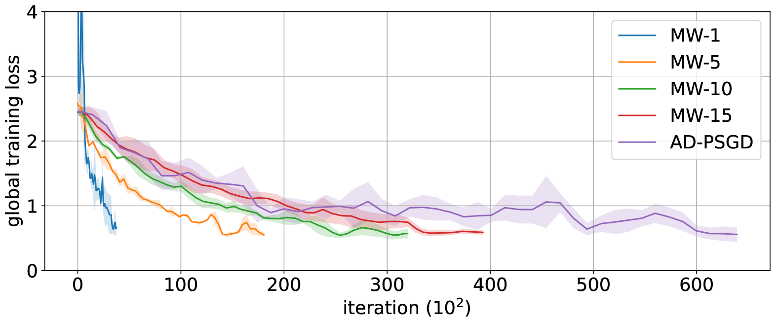
(a) Cycle graph.

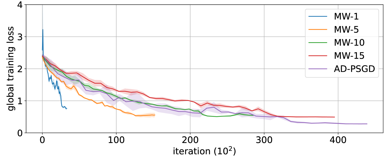
(b) Complete graph.

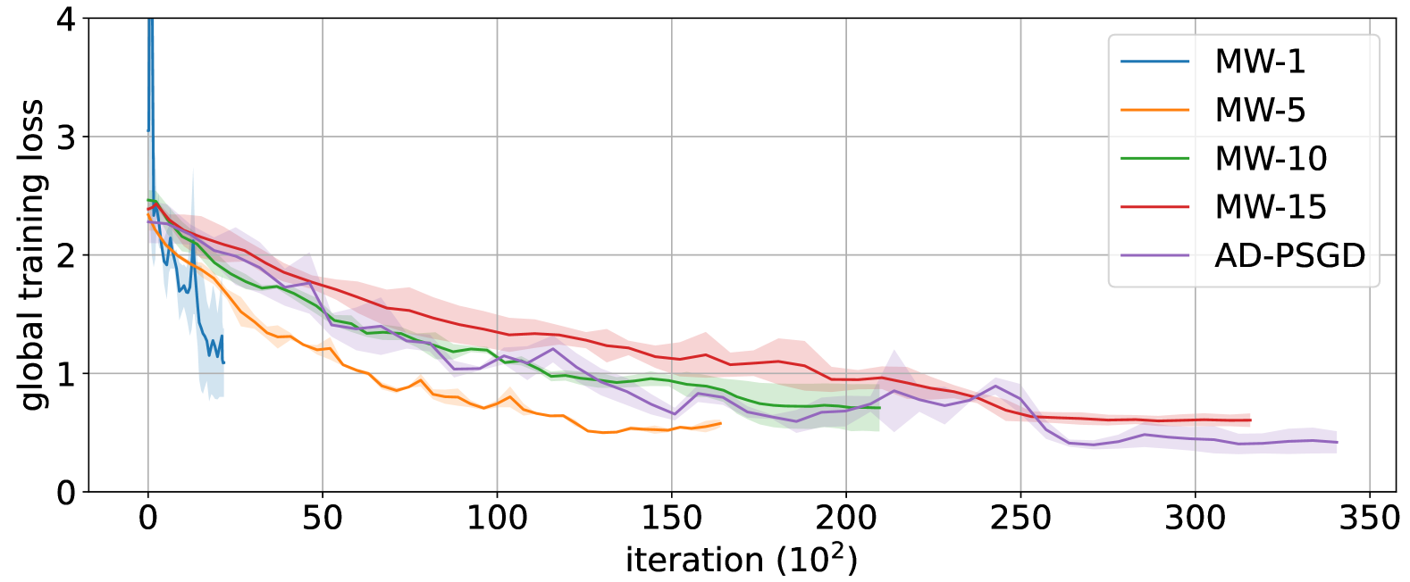
(c) Erdős–Rényi ($0.3$) graph.

Figure 2: Training loss of ResNet-$20$ on Cifar-$10$ on a $20$-node graph with different topologies.

In this section, we aim to validate our theoretical results through empirical experiments, which include the following:

• Section 5.1 verifies the impact of network topology on the convergence rate.

• Section 5.2 explores the impact of data heterogeneity on the convergence rate.

• Section 5.3 validates communication efficiency of MW for a large language model (LLM).

We use two machine learning tasks: (i) Image classification on CIFAR-$10$ (Krizhevsky, 2009) using ResNet-$20$ (He et al., 2015); and (ii) LLM fine-tuning of OPT-$125$M (Zhang et al., 2022) as a large language model on the Multi-Genre Natural Language Inference (MultiNLI) corpus (Williams et al., 2018). We repeat each experiment $10$ times and present the error bars associated with the randomness of the optimization. In every figure, we include the average and standard deviation error bars. We have conducted the experiments on the National Resource Platform (NRP) (San Diego Supercomputer Center, ) cluster. Detailed experimental setup is provided in Appendix E of the supplementary materials.

We use the Dirichlet distribution to create disjoint non-iid nodes (Lin et al., 2021). The degree of data heterogeneity is controlled by the distribution parameter $\alpha$; the smaller $\alpha$ is, the more likely the nodes hold examples from only one class. Throughout the experiments, we use three levels of $\alpha$; $10$, $1$, and $0.1$. The distribution of data for each case is shown in Appendix E.1.

5.1 Graph topology

In Figure 2, we observe the training loss of the image classification task in a graph of $20$ nodes. We consider three topologies of cycle, complete, and Erdős–Rényi with connection probability of each pair of nodes being $0.3$. The noniid-ness level for this experiment is set to $\alpha=1$. We observe in Figure 2(a) that the convergence rate w.r.t iterations in cycle topology is faster for MW, regardless of the number of walks ($R$), MW is outperforming Asynchronous Gossip. We also observe that as we decrease $R$, MW convergence rate w.r.t iterations improves. Increasing the number of walks improves the performance in time domain, as we observe in section 5.2. When we decrease the diameter of the topology by going to complete graph in Figure 2(b), we observe that MW no longer is superior and Asynchronous Gossip is outperforming MW with $15$ walks. Here in Figure 2(c), we have the results for an Erdős–Rényi topology with the connection probability of $0.3$. This topology, where each node is connected to every other node with a probability of $0.3$, is a well-connected graph with a small diameter. We observe that the Erdős–Rényi graph results are quite similar to the complete graph.

5.2 Noniid-ness

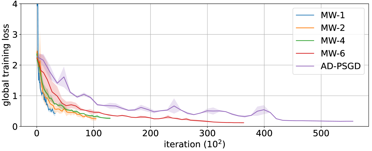
(a) $\alpha=10$, w.r.t iterations.

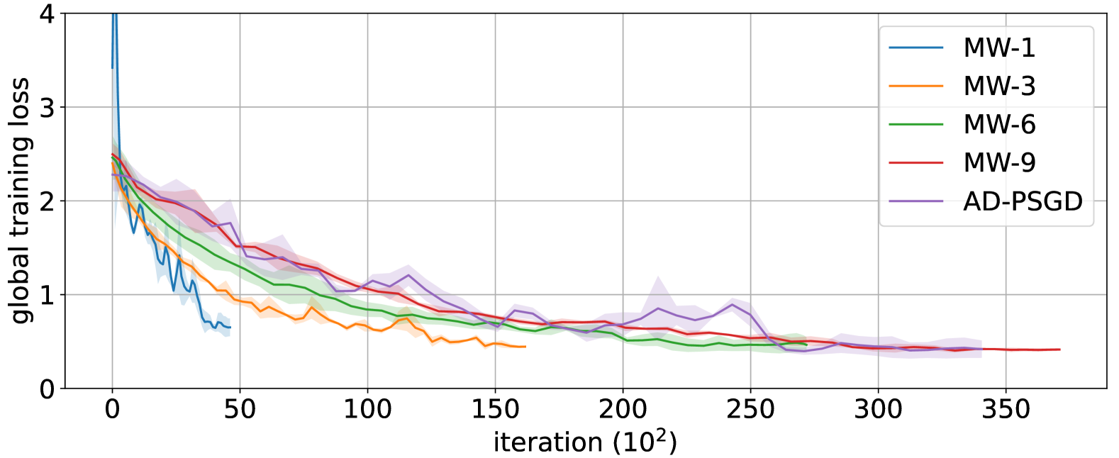
(b) $\alpha=1$, w.r.t iterations.

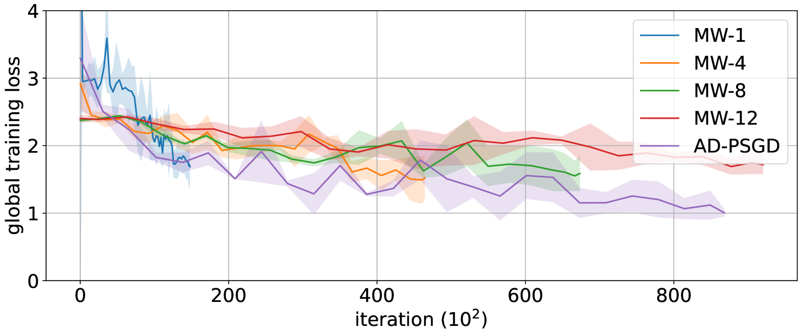
(c) $\alpha=0.1$, w.r.t iterations.

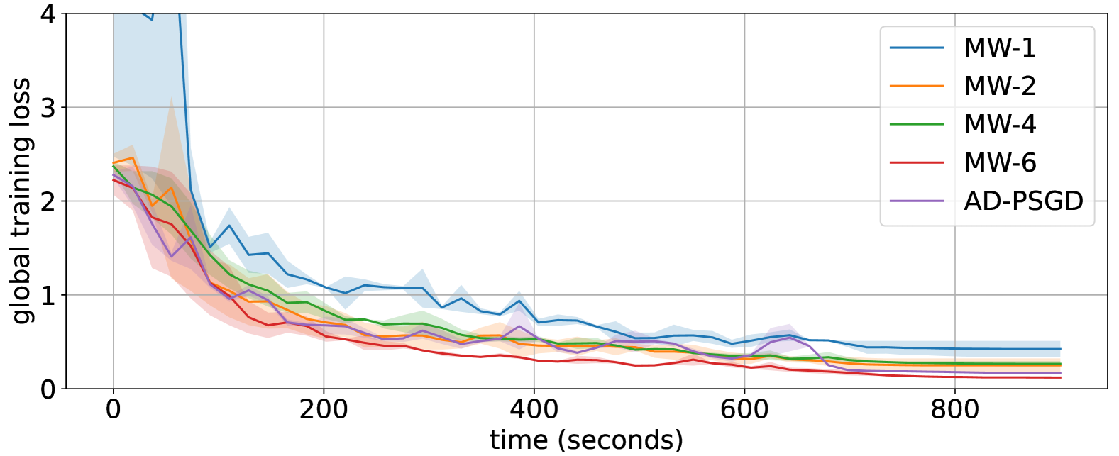
(d) $\alpha=10$, w.r.t wall-clock time.

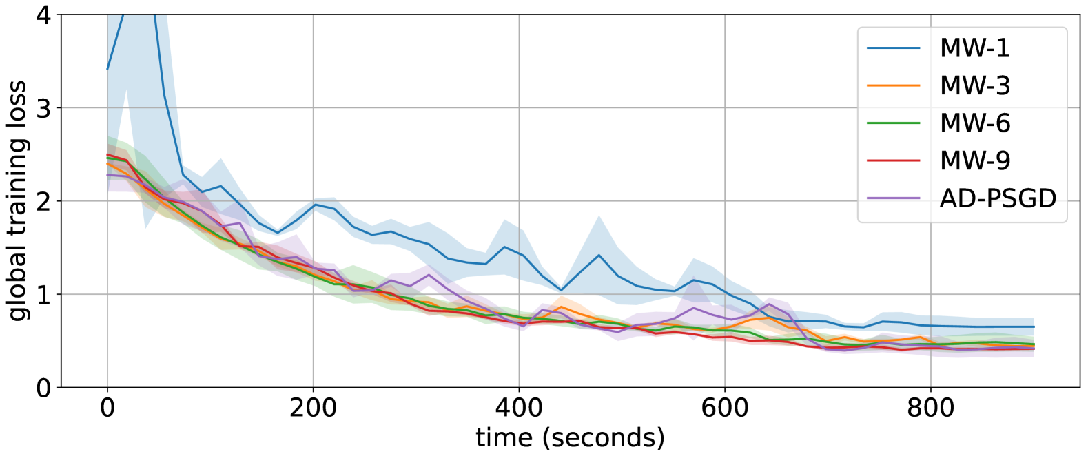
(e) $\alpha=1$, w.r.t wall-clock time.

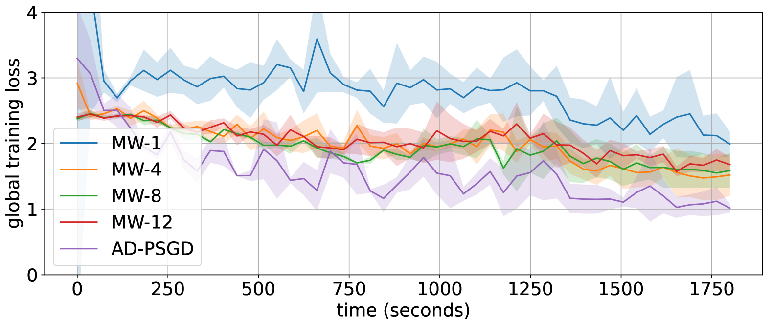
(f) $\alpha=0.1$, w.r.t wall-clock time.

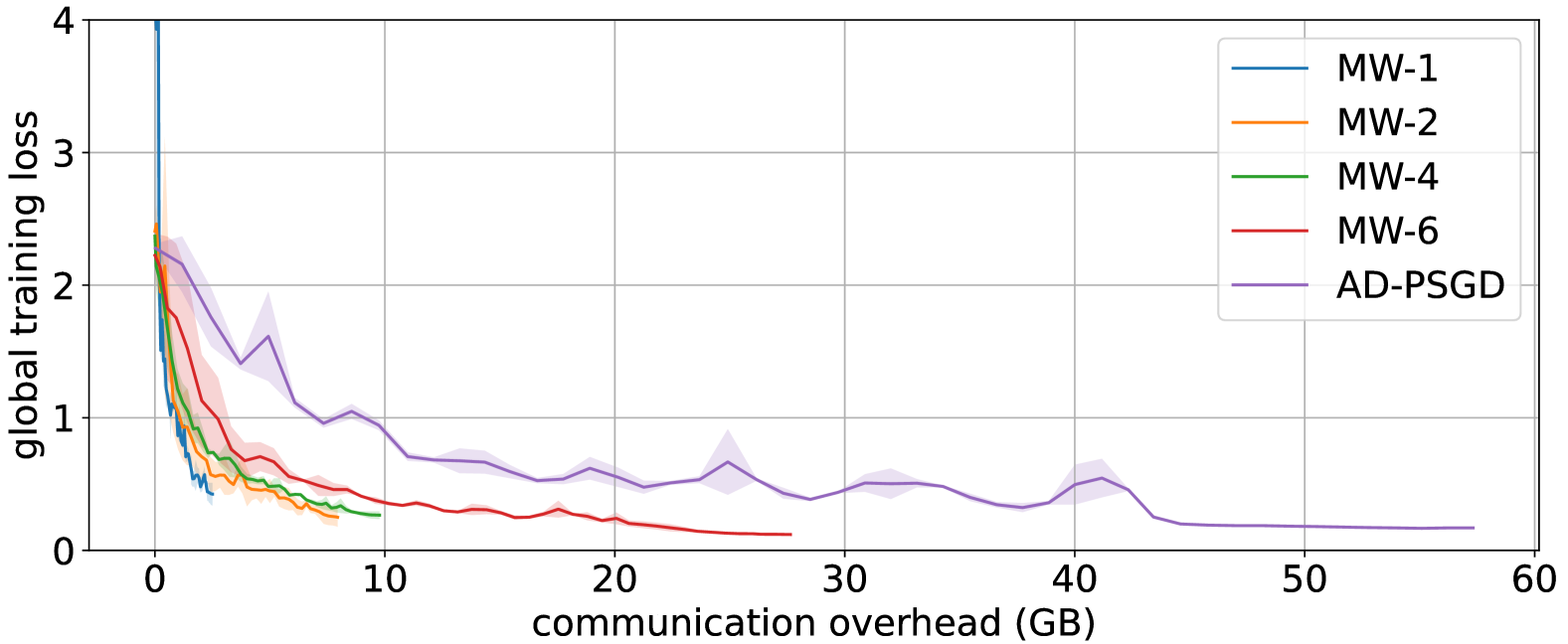
(g) $\alpha=10$, w.r.t transmitted bits.

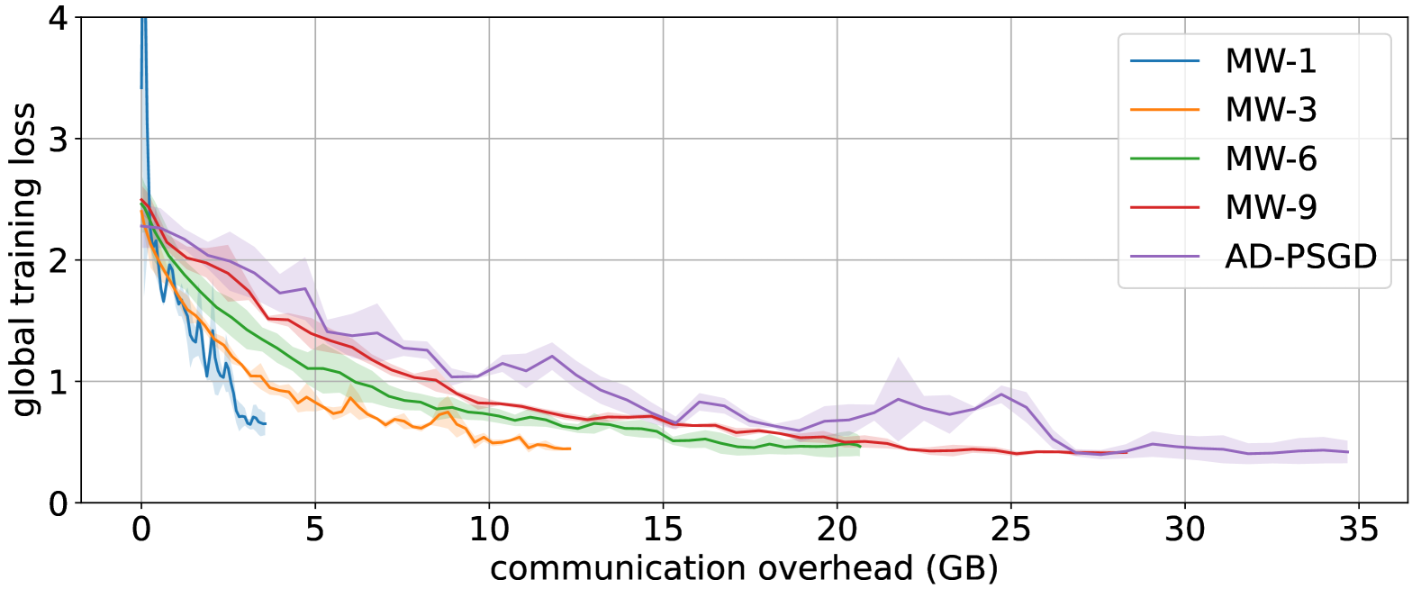
(h) $\alpha=1$, w.r.t transmitted bits.

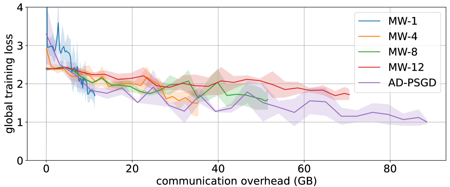
(i) $\alpha=0.1$, w.r.t transmitted bits.

Figure 3: Training of ResNet-$20$ on Cifar-$10$ on and $20$-node Erdős–Rényi ($0.3$) graph for different levels of noniid-ness.

Figure 3 shows the results for a 20-node Erdős–Rényi ($0.3$) graph under different levels of noniid-ness. The first row (a, b, c) shows the convergence w.r.t iterations, the second row (d, e, f) shows the convergence w.r.t wall-clock time, and the third row (g, h, i) shows the convergence w.r.t transmitted bits. We observed in section 5.1 that Erdős–Rényi ($0.3$) has a quite small diameter. We also saw earlier in the theories that in such graphs with small diameters, increasing the level of noniid-ness degrades MW with more strength than Asynchronous Gossip. This suggests that if we increase the level of non-iidness MW gets more impacted adversely. In Figure 3(a), the value of $\alpha$ is $10$, and the data distribution is quite iid, MW outperforms Asynchronous Gossip w.r.t iteration. We know that when going to time domain Asynchronous Gossip enjoys a linear speed-up with a number of nodes; this is shown in Figure 3(d) that compensates the superiority of MW w.r.t iterations.

If we decrease the value of $\alpha$ to $1$, introducing more noniid-ness, we observe w.r.t iterations MW’s performance is worse than Asynchronous Gossip in Figure 3(b). We can go further and reduce $\alpha$ to $0.1$ to get extreme non-iid data distribution. Here, we observe that Asynchronous Gossip is better even w.r.t iteration. This is expected because we had in Table 2 that in MW $\zeta^{2}$ is multiplied with $H^{2}$ (for a small diameter graph like complete $H^{2}=\mathcal{O}(V^{2})$) while in Asynchronous Gossip is multiplied with $1/{p^{2}}$ (for a small diameter graph like complete $p=1$). This suggests the impact of noniid-ness in small-diameter topologies is more severe on MW than Asynchronous Gossip, which is verified with this experiment.

In terms of communication overhead, we observe that in settings that are not extremely non-iid, where the dominating term is the largest, MW outperforms Asynchronous Gossip as predicted by the results in Table 3 (Figures 3(g), 3(h)). However, in the extreme non-iid setting of Figure 3(i), the value of $\zeta$ becomes too large that the second dominating term in Table 3 comes into play. In this term, the impact of noniid-ness in a graph topology with a small diameter significantly disfavors MW, which is evident from the observed results. We have presented the same experiment results for cycle topology in Appendix F that shows in MW still outperforms in extreme noniid-ness.

5.3 Communication restricted settings

In Figure 4, we observe the loss of fine-tuning OPT-$125$M on the MultiNLI corpus in an Erdős–Rényi ($0.3$) graph with 20 nodes. Compared to ResNet-$20$, which requires only $1.08$ MB, OPT-$125$M requires $500$ MB of data transmission per communication round when each parameter is stored as a standard $32$-bit floating-point value.

In Figure 4(a), the horizontal axis represents the total communicated bits during fine-tuning. We observe that while MW with a single walk requires approximately $50$ GB to converge, Asynchronous Gossip requires around $600$ GB. We have also presented the convergence w.r.t wall-clock time in Figure 4(b). Although Asynchronous Gossip benefits from linear speedup due to the increased number of active nodes, MW still outperforms it. This is because, as the model size increases, using Asynchronous Gossip with numerous concurrent communications in the network leads to congestion, which, in turn, increases the average communication delay across network links. Consequently, this results in a larger $d$ i.e., the average computation and gossip communication delay in the system, making Asynchronous Gossip slower with respect to wall-clock time as well. We observe that in such settings where communication resources are restricted MW is promising.

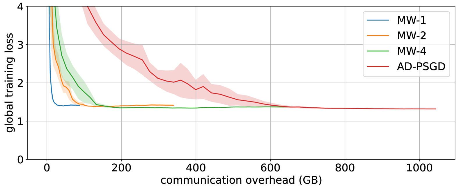
(a) w.r.t transmitted bits.

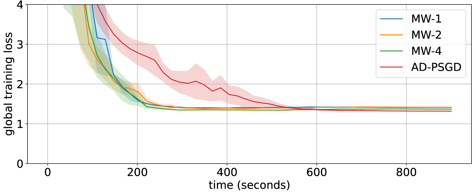
(b) w.r.t wall-clock time.

Figure 4: Fine-tuning OPT-$125$M on the MultiNLI corpus in a $20$-node Erdős–Rényi ($0.3$) graph.

6 Conclusion

We presented a comprehensive analysis of the two most prominent approaches in decentralized learning: gossip-based and random walk-based algorithms. Generally, gossip-based methods are advantageous in topologies with a small diameter, while random walk-based approaches perform better in large-diameter topologies. We also showed that increasing heterogeneity in data distribution impacts random walk-based methods more severely than gossip-based approaches especially in small-diameter topologies.

Impact Statement

This paper presents work whose goal is to advance the field of Machine Learning. There are many potential societal consequences of our work, none which we feel must be specifically highlighted here.

Appendix A Notation Table

$G=(\mathcal{V},\xi)$	The graph representing the network
$V$	Number of nodes
$\mathcal{D}_{v}$	Local dataset at node $v$
$F_{v}(\mathbf{x},\xi)$	Loss function of $\mathbf{x}$ associated with the data sample $\xi$ at node $v$
$f(\mathbf{x})$	Global loss function of model $\mathbf{x}$
$f_{v}(\mathbf{x})$	Local loss function of model $\mathbf{x}$ on local dataset $\mathcal{D}_{v}$ at node $v$
$f^{*}$	$\min_{\mathbf{x}\in\mathbb{R}^{d}}f(\mathbf{x})$
$\mathbf{x}_{0}$	Initial model
$T$	Total number of iterations
$\eta_{t}$	Learning rate at iteration $t$
$\mathbf{x}^{r}_{t}$	Model of walk $r$ at iteration $t$ in MW Algorithm
$\mathbf{x}^{v}_{t}$	Local model of node $v$ at iteration $t$ in Asynchronous Gossip Algorithm
$u^{r}$	A copy of the model of walk $r$ at the most recent instance when that walk was at Node $0$ in MW Algorithm; to be kept at Node $0$
$l$	The index of the latest walk visited Node $0$ in MW Algorithm
$\mathbf{P}$	The transition matrix of each walk in MW, and in Asynchronous Gossip, it defines the mixing step of the gossip process
$p_{ij}$	The element in row $i$ and column $j$ of $\mathbf{P}$
$p$	The spectral gap of $\mathbf{P}^{\top}\mathbf{P}$
$p^{\prime}$	The spectral gap of $\mathbf{P}$
$m$	Model size in bits
$B$	Total transmitted bits
$Z$	Wall-clock time
$L$	$f_{v}(\mathbf{x})$’s gradient is $L$-Lipschitz
$\sigma^{2}$	Upper Bound for local variance
$\zeta^{2}$	Upper Bound for diversity
$F$	$f(\mathbf{x}_{0})-f^{*}$
$H^{2}$	The second moment of the first return time to Node $0$ for the Markov chain representing each walk
$\alpha$	The degree of noniid-ness in the Dirichlet distribution is used to create disjoint noniid nodes; smaller values indicate a higher level of noniid-ness

Appendix B Proof of Theorem 4.1

Motivated by (Stich, 2019), a virtual sequence $\{\tilde{\mathbf{x}}_{t}\}_{t\geq 0}$ is defined as follows.

$$\tilde{\mathbf{x}}_{t+1}=\tilde{\mathbf{x}}_{t}-\frac{\eta}{R}\nabla F_{v_{t}}(\mathbf{x}^{r_{t}}_{t},\xi_{t+\hat{\tau}_{t}}),$$ (5)

where we define $\hat{\tau}_{t}$ as the delay with which the gradient of the corresponding point $(\mathbf{x}^{r_{t}}_{t})$ will be computed. If we denote $t^{\prime}=t+\hat{\tau}_{t}$, then it holds that $t^{\prime}-\tau_{t^{\prime}}=t$. We do not need to calculate this sequence in the algorithm explicitly and it is only used for the sake of analysis.

First, we illustrate how the virtual sequence, $\{\tilde{\mathbf{x}}_{t}\}_{t\geq 0}$, approaches to the optimal. Second, we depict that there is a little deviation from the virtual sequence in the actual iterates, $\mathbf{x}^{r_{t}}_{t}$. Finally, the convergence rate is proved.

Lemma B.1 (Descent Lemma for Multi-Walk).

Under Assumptions 1, 2, 3, and learning rate $\eta\leq\frac{R}{6L}$, it holds that

$$\operatorname{\mathbb{E}}f(\tilde{\mathbf{x}}_{t+1})\leq f(\tilde{\mathbf{x}}_{t})-\frac{\eta}{4R}\|\nabla f(\mathbf{x}^{r_{t}}_{t})\|^{2}+\frac{2c\eta}{R}\zeta^{2}(1-p^{\prime})^{2|\mathcal{T}_{r_{t}}|}+\frac{3\eta^{2}L^{2}}{2R^{2}}\left(\sigma^{2}+\zeta^{2}\right)+\frac{\eta L^{2}}{2R}\|\tilde{\mathbf{x}}_{t}-\mathbf{x}^{r_{t}}_{t}\|^{2},$$ (6)

where $\mathcal{T}_{r_{t}}=\{t^{\prime}\leq t:r_{t^{\prime}}=r_{t}\}$.

Proof.

Based on the definition of $\tilde{\mathbf{x}}_{t}$ and $L$-smoothness of $f(\mathbf{x})$ we have

$$f(\tilde{\mathbf{x}}_{t+1}) =f(\tilde{\mathbf{x}}_{t}-\frac{\eta}{R}\nabla F_{v_{t}}(\mathbf{x}^{r_{t}}_{t},\xi_{t+\hat{\tau}_{t}}))$$ (7)

$$\leq f(\tilde{\mathbf{x}}_{t})+\frac{\eta}{R}\langle\nabla f(\tilde{\mathbf{x}}_{t}),-\nabla F_{v_{t}}(\mathbf{x}^{r_{t}}_{t},\xi_{t+\hat{\tau}_{t}})\rangle+\frac{\eta^{2}L}{2R^{2}}\|\nabla F_{v_{t}}(\mathbf{x}^{r_{t}}_{t},\xi_{t+\hat{\tau}_{t}})\|^{2}.$$ (8)

Lets take expectation of the second term on the right-hand side of (8).

$$\frac{\eta}{R}\operatorname{\mathbb{E}} \langle\nabla f(\tilde{\mathbf{x}}_{t}),-\nabla F_{v_{t}}(\mathbf{x}^{r_{t}}_{t},\xi_{t+\hat{\tau}_{t}})\rangle$$ (9)

$$=\frac{\eta}{R}\operatorname{\mathbb{E}}_{v_{t}}\operatorname{\mathbb{E}}_{\xi_{t+\hat{\tau}_{t}}}\langle\nabla f(\tilde{\mathbf{x}}_{t}),-\nabla F_{v_{t}}(\mathbf{x}^{r_{t}}_{t},\xi_{t+\hat{\tau}_{t}})\rangle$$ (10)

$$=\frac{\eta}{R}\operatorname{\mathbb{E}}_{v_{t}}\langle\nabla f(\tilde{\mathbf{x}}_{t}),-\nabla f_{v_{t}}(\mathbf{x}^{r_{t}}_{t})\rangle$$ (11)

$$=\frac{\eta}{R}\langle\nabla f(\tilde{\mathbf{x}}_{t}),-\operatorname{\mathbb{E}}_{v_{t}}\nabla f_{v_{t}}(\mathbf{x}^{r_{t}}_{t})\rangle$$ (12)

$$=\frac{\eta}{R}\langle\nabla f(\tilde{\mathbf{x}}_{t}),-\nabla f(\mathbf{x}^{r_{t}}_{t})+\nabla f(\mathbf{x}^{r_{t}}_{t})-\operatorname{\mathbb{E}}_{v_{t}}\nabla f_{v_{t}}(\mathbf{x}^{r_{t}}_{t})\rangle$$ (13)

$$=\frac{\eta}{R}\underbrace{\langle\nabla f(\tilde{\mathbf{x}}_{t}),-\nabla f(\mathbf{x}^{r_{t}}_{t})\rangle}_{=:T_{1}}+\frac{\eta}{R}\underbrace{\langle\nabla f(\tilde{\mathbf{x}}_{t}),\nabla f(\mathbf{x}^{r_{t}}_{t})-\operatorname{\mathbb{E}}_{v_{t}}\nabla f_{v_{t}}(\mathbf{x}^{r_{t}}_{t})\rangle}_{=:T_{2}}.$$ (14)

We estimate $T_{1}$ and $T_{2}$ separately.

$$T_{1} =-\frac{1}{2}\|\nabla f(\tilde{\mathbf{x}}_{t})\|^{2}-\frac{1}{2}\|\nabla f(\mathbf{x}^{r_{t}}_{t})\|^{2}+\frac{1}{2}\|\nabla f(\tilde{\mathbf{x}}_{t})-\nabla f(\mathbf{x}^{r_{t}}_{t})\|^{2}.$$ (15)

We also obtain

$$T_{2} \leq\frac{1}{2}\|\nabla f(\tilde{\mathbf{x}}_{t})\|^{2}+\frac{1}{2}\|\operatorname{\mathbb{E}}_{v_{t}}\left[\nabla f_{v_{t}}(\mathbf{x}^{r_{t}}_{t})-f(\mathbf{x}^{r_{t}}_{t})\right]\|^{2}$$ (16)

$$=\frac{1}{2}\|\nabla f(\tilde{\mathbf{x}}_{t})\|^{2}+\frac{1}{2}\|\sum_{v=1}^{V}P_{v}^{t}\left(\nabla f_{v_{t}}(\mathbf{x}^{r_{t}}_{t})-f(\mathbf{x}^{r_{t}}_{t})\right)\|^{2}$$ (17)

$$=\frac{1}{2}\|\nabla f(\tilde{\mathbf{x}}_{t})\|^{2}+\frac{1}{2}\|\sum_{v=1}^{V}(P_{v}^{t}-\pi_{v})\left(\nabla f_{v_{t}}(\mathbf{x}^{r_{t}}_{t})-f(\mathbf{x}^{r_{t}}_{t})\right)\|^{2}$$ (18)

$$\leq\frac{1}{2}\|\nabla f(\tilde{\mathbf{x}}_{t})\|^{2}+\frac{1}{2}\left(\sum_{v=1}^{V}|P_{v}^{t}-\pi_{v}|\|\nabla f_{v_{t}}(\mathbf{x}^{r_{t}}_{t})-f(\mathbf{x}^{r_{t}}_{t})\|\right)^{2}$$ (19)

$$\leq\frac{1}{2}\|\nabla f(\tilde{\mathbf{x}}_{t})\|^{2}+\frac{1}{2}\zeta^{2}\left(\sum_{v=1}^{V}|P_{v}^{t}-\pi_{v}|\right)^{2}$$ (20)

$$\leq\frac{1}{2}\|\nabla f(\tilde{\mathbf{x}}_{t})\|^{2}+\frac{1}{2}\zeta^{2}\left(2\|P^{t}-\pi\|_{TV}\right)^{2}$$ (21)

$$\leq\frac{1}{2}\|\nabla f(\tilde{\mathbf{x}}_{t})\|^{2}+2c\zeta^{2}(1-p^{\prime})^{2|\mathcal{T}_{r_{t}}|},$$ (22)

where (16) is based on the fact that for any $\lambda>0$,

$$2\langle a,b\rangle\leq\lambda\|a\|^{2}+\frac{1}{\lambda}\|b\|^{2}.$$ (23)

$P_{v}^{t}$ shows the probability of being at node $v$ at iteration $t$ and $\pi_{v}$ is the steady state distribution of node $v$. In (21) we have used the fact that the total variation distance between two probability distributions $\mu$ and $\nu$ on $\mathcal{X}$ satisfies

$$\|\mu-\nu\|_{TV}=\frac{1}{2}\sum_{x\in\mathcal{X}}|\mu(x)-\nu(x)|.$$ (24)

(22) is based on the following well-known bound on the mixing time for a Markov chain (see, for example, Guruswami (2016); Levin & Peres (2017)).

$$\|P^{t}-\pi\|_{TV}\leq c(1-p^{\prime})^{|\mathcal{T}_{r_{t}}|},$$ (25)

where $\mathcal{T}_{r_{t}}=\{t^{\prime}\leq t:r_{t^{\prime}}=r_{t}\}$ is the set of all iteration on walk $r_{t}$. $(1-p^{\prime})$ is the second largest eigenvalue of matrix $\mathbf{P}$ representing the irreducible aperiodic Markov chain of each walk and $c>0$ is a constant.

So we get

$$\frac{\eta}{R}\operatorname{\mathbb{E}} \langle\nabla f(\tilde{\mathbf{x}}_{t}),-\nabla F_{v_{t}}(\mathbf{x}^{r_{t}}_{t},\xi_{t+\hat{\tau}_{t}})\rangle\leq-\frac{\eta}{2R}\|\nabla f(\mathbf{x}^{r_{t}}_{t})\|^{2}+\frac{\eta}{2R}\|\nabla f(\tilde{\mathbf{x}}_{t})-\nabla f(\mathbf{x}^{r_{t}}_{t})\|^{2}+\frac{2c\eta}{R}\zeta^{2}(1-p^{\prime})^{2|\mathcal{T}_{r_{t}}|}.$$ (26)

Now we derive expectation of the last term on the right-hand side of (8).

$$\operatorname{\mathbb{E}}\|\nabla F_{v_{t}}(\mathbf{x}^{r_{t}}_{t},\xi_{t+\hat{\tau}_{t}})\|^{2} =\operatorname{\mathbb{E}}\|\nabla F_{v_{t}}(\mathbf{x}^{r_{t}}_{t},\xi_{t+\hat{\tau}_{t}})\pm\nabla f_{v_{t}}(\mathbf{x}^{r_{t}}_{t})\pm\nabla f(\mathbf{x}^{r_{t}}_{t})\|^{2}$$ (27)

$$\leq 3\operatorname{\mathbb{E}}\|\nabla F_{v_{t}}(\mathbf{x}^{r_{t}}_{t},\xi_{t+\hat{\tau}_{t}})-\nabla f_{v_{t}}(\mathbf{x}^{r_{t}}_{t})\|^{2}+3\operatorname{\mathbb{E}}\|\nabla f_{v_{t}}(\mathbf{x}^{r_{t}}_{t})-\nabla f(\mathbf{x}^{r_{t}}_{t})\|^{2}+3\|\nabla f(\mathbf{x}^{r_{t}}_{t})\|^{2}$$ (28)

$$\leq 3\sigma^{2}+3\zeta^{2}+3\|\nabla f(\mathbf{x}^{r_{t}}_{t})\|^{2},$$ (29)

where (28) is based on the following inequality.

$$\|\sum_{i=1}^{n}\mathbf{a}_{i}\|^{2}\leq n\sum_{i=1}^{n}\|\mathbf{a}_{i}\|^{2}.$$ (30)

Combining these together and using $L$-smoothness to estimate $\|\nabla f(\tilde{\mathbf{x}}_{t})-\nabla f(\mathbf{x}^{r_{t}}_{t})\|^{2}$ we obtain

$$\operatorname{\mathbb{E}}f(\tilde{\mathbf{x}}_{t+1})\leq f(\tilde{\mathbf{x}}_{t})-\left(\frac{\eta}{2R}-\frac{3\eta^{2}L}{2R^{2}}\right)\|\nabla f(\mathbf{x}^{r_{t}}_{t})\|^{2}+\frac{\eta L^{2}}{2R}\|\tilde{\mathbf{x}}_{t}-\mathbf{x}^{r_{t}}_{t}\|^{2}+\frac{2c\eta}{R}\zeta^{2}(1-p^{\prime})^{2|\mathcal{T}_{r_{t}}|}+\frac{3\eta^{2}L}{2R^{2}}\left(\sigma^{2}+\zeta^{2}\right).$$ (31)

Considering $\eta\leq\frac{R}{6L}$ we obtain

$$\operatorname{\mathbb{E}}f(\tilde{\mathbf{x}}_{t+1})\leq f(\tilde{\mathbf{x}}_{t})-\frac{\eta}{4R}\|\nabla f(\mathbf{x}^{r_{t}}_{t})\|^{2}+\frac{\eta L^{2}}{2R}\|\tilde{\mathbf{x}}_{t}-\mathbf{x}^{r_{t}}_{t}\|^{2}+\frac{2c\eta}{R}\zeta^{2}(1-p^{\prime})^{2|\mathcal{T}_{r_{t}}|}+\frac{3\eta^{2}L}{2R^{2}}\left(\sigma^{2}+2\zeta^{2}\right).$$ (32)

∎

Lemma B.2 (Bounding Deviation for Multi-Walk).

Under Assumptions 2, 3, 4, and learning rate $\eta\leq\frac{1}{7LH}$, it holds that

$$\frac{1}{T}\sum_{t=1}^{T}\operatorname{\mathbb{E}}\|\tilde{\mathbf{x}}_{t}-\mathbf{x}^{r_{t}}_{t}\|^{2}\leq 12V\sigma^{2}\eta^{2}+12H^{2}\zeta^{2}\eta^{2}+\frac{1}{4L^{2}T}\sum_{t=1}^{T-1}\operatorname{\mathbb{E}}\|\nabla f(\mathbf{x}^{r_{t}}_{t})\|^{2},$$ (33)

where $H^{2}$ is the second moment of the first return time to the Node $0$.

Proof.

First we define $l^{r}_{t}$ as the last iteration before $t$ when walk $r$ has visited Node $0$, i.e., $l^{r}_{t}=\max\{t^{\prime}\mid t^{\prime}\leq t,r_{t}=r,v_{t}=0\}$.

$$\operatorname{\mathbb{E}}\|\tilde{\mathbf{x}}_{t}-\mathbf{x}^{r_{t}}_{t}\|^{2} =\operatorname{\mathbb{E}}\|\sum_{z=l^{r}_{l^{r_{t}}_{t}},r_{z}\neq r_{t}}^{t-1}-\frac{\eta}{R}\nabla F_{v_{z}}(\mathbf{x}^{r_{z}}_{z},\xi_{z+\hat{\tau}_{z}})+\sum_{z=l^{r_{t}}_{t},r_{z}=r_{t}}^{t-1}\left(1-\frac{1}{R}\right)\eta\nabla F_{v_{z}}(\mathbf{x}^{r_{z}}_{z},\xi_{z+\hat{\tau}_{z}})\|^{2}$$ (34)

$$\leq\frac{2}{R^{2}}\operatorname{\mathbb{E}}\|\sum_{z=l^{r}_{l^{r_{t}}_{t}},r_{z}\neq r_{t}}^{t-1}\eta\nabla F_{v_{z}}(\mathbf{x}^{r_{z}}_{z},\xi_{z+\hat{\tau}_{z}})\|^{2}+2\operatorname{\mathbb{E}}\|\sum_{z=l^{r_{t}}_{t},r_{z}=r_{t}}^{t-1}\eta\nabla F_{v_{z}}(\mathbf{x}^{r_{z}}_{z},\xi_{z+\hat{\tau}_{z}})\|^{2}$$ (35)

$$\leq\underbrace{\frac{2}{R^{2}}\operatorname{\mathbb{E}}\|\sum_{z\in U^{1}_{t}}\eta\nabla F_{v_{z}}(\mathbf{x}^{r_{z}}_{z},\xi_{z+\hat{\tau}_{z}})\|^{2}}_{:=T_{1}}+\underbrace{2\operatorname{\mathbb{E}}\|\sum_{z\in U^{2}_{t}}\eta\nabla F_{v_{z}}(\mathbf{x}^{r_{z}}_{z},\xi_{z+\hat{\tau}_{z}})\|^{2}}_{:=T_{2}},$$ (36)

where $U^{1}_{t}=\{l^{r}_{l^{r_{t}}_{t}}\leq z\leq t-1\mid r_{z}\neq r_{t}\}$, and $U^{2}_{t}=\{l^{r_{t}}_{t}\leq z\leq t-1\mid r_{z}=r_{t}\}$.

We have

$$\nabla F_{v_{t}}(\mathbf{x}^{r_{t}}_{t},\xi_{t+\hat{\tau}_{t}})=\left(\nabla F_{v_{t}}(\mathbf{x}^{r_{t}}_{t},\xi_{t+\hat{\tau}_{t}})-\nabla f_{v_{t}}(\mathbf{x}^{r_{t}}_{t})\right)+\left(\nabla f_{v_{t}}(\mathbf{x}^{r_{t}}_{t})-\nabla f(\mathbf{x}^{r_{t}}_{t})\right)+\nabla f(\mathbf{x}^{r_{t}}_{t}).$$ (37)

So, based on (30) we can write

$$T_{1} \leq\frac{6}{R^{2}}\operatorname{\mathbb{E}}\biggl{(}\|\sum_{z\in U^{1}_{t}}\eta\left(\nabla F_{v_{z}}(\mathbf{x}^{r_{z}}_{z},\xi_{z+\hat{\tau}_{z}})-\nabla f_{v_{z}}(\mathbf{x}^{r_{z}}_{z})\right)\|^{2}+\|\sum_{z\in U^{1}_{t}}\eta\left(\nabla f_{v_{z}}(\mathbf{x}^{r_{z}}_{z})-\nabla f(\mathbf{x}^{r_{z}}_{z})\right)\|^{2}$$ (38)

$$\mathllap{+\|\sum_{z\in U^{1}_{t}}\eta\nabla f(\mathbf{x}^{r_{z}}_{z})\|^{2}\biggl{)}}$$

$$\leq\frac{6}{R^{2}}\operatorname{\mathbb{E}}\left(\sum_{z\in U^{1}_{t}}\eta^{2}\sigma^{2}+|U^{1}_{t}|\sum_{z\in U^{1}_{t}}\eta^{2}\zeta^{2}+|U^{1}_{t}|\sum_{z\in U^{1}_{t}}\eta^{2}\|\nabla f(\mathbf{x}^{r_{z}}_{z})\|^{2}\right),$$ (39)

where in (39) we have applied (30) and the fact that for independent zero-mean random variables, we get a tighter bound as follows.

$$\operatorname{\mathbb{E}}\|\sum_{i=1}^{n}\mathbf{a}_{i}\|^{2}\leq\sum_{i=1}^{n}\operatorname{\mathbb{E}}\|\mathbf{a}_{i}\|^{2}.$$ (40)

Averaging over $T$, we get

$$\frac{1}{T}\sum_{t=1}^{T-1}T_{1} \leq\frac{6}{TR^{2}}\operatorname{\mathbb{E}}\left(\sum_{t=1}^{T-1}\sum_{z\in U^{1}_{t}}\eta^{2}\sigma^{2}+\sum_{t=1}^{T-1}|U^{1}_{t}|\sum_{z\in U^{1}_{t}}\eta^{2}\zeta^{2}+\sum_{t=1}^{T-1}|U^{1}_{t}|\sum_{z\in U^{1}_{t}}\eta^{2}\|\nabla f(\mathbf{x}^{r_{z}}_{z})\|^{2}\right)$$ (41)

$$\leq\frac{6}{TR^{2}}\operatorname{\mathbb{E}}\left(\sum_{t=1}^{T-1}|U^{1}_{t}|\eta^{2}\sigma^{2}+\sum_{t=1}^{T-1}|U^{1}_{t}|^{2}\eta^{2}\zeta^{2}+\sum_{t=1}^{T-1}|U^{1}_{t}|\sum_{z\in U^{1}_{t}}\eta^{2}\|\nabla f(\mathbf{x}^{r_{z}}_{z})\|^{2}\right)$$ (42)

$$\leq\frac{6}{TR^{2}}\operatorname{\mathbb{E}}\left(\sum_{t=1}^{T-1}(R-1)h\eta^{2}\sigma^{2}+\sum_{t=1}^{T-1}(R-1)^{2}h^{2}\eta^{2}\zeta^{2}+(R-1)h\eta^{2}\sum_{t=1}^{T-1}\sum_{z\in U^{1}_{t}}\|\nabla f(\mathbf{x}^{r_{z}}_{z})\|^{2}\right)$$ (43)

$$\leq\frac{6}{TR^{2}}\operatorname{\mathbb{E}}\left(\sum_{t=1}^{T-1}(R-1)h\eta^{2}\sigma^{2}+\sum_{t=1}^{T-1}(R-1)^{2}h^{2}\eta^{2}\zeta^{2}+(R-1)^{2}h^{2}\eta^{2}\sum_{t=1}^{T-1}\|\nabla f(\mathbf{x}^{r_{t}}_{t})\|^{2}\right)$$ (44)

$$\leq\frac{6}{TR^{2}}\left(\sum_{t=1}^{T-1}\left(R-1\right)V\eta^{2}\sigma^{2}+\sum_{t=1}^{T-1}\left(R-1\right)^{2}H^{2}\eta^{2}\zeta^{2}+\sum_{t=1}^{T-1}\left(R-1\right)^{2}H^{2}\eta^{2}\operatorname{\mathbb{E}}\|\nabla f(\mathbf{x}^{r_{z}}_{z})\|^{2}\right)$$ (45)

$$\leq\frac{6}{T}\left(\sum_{t=1}^{T-1}\frac{V}{R}\eta^{2}\sigma^{2}+\sum_{t=1}^{T-1}H^{2}\eta^{2}\zeta^{2}+\sum_{t=1}^{T-1}H^{2}\eta^{2}\operatorname{\mathbb{E}}\|\nabla f(\mathbf{x}^{r_{t}}_{t})\|^{2}\right),$$ (46)

where in (43) and (44), we have used the fact that $|U^{1}_{t}|$ is upper bounded with $R-1$ times the first return time to Node $0$ ($h$). Expectation of the first return time is $\frac{1}{\pi_{0}}=V$ and the second moment of this random variable is assumed $H^{2}$ that are applied in (45).

Following the same approach for $T_{2}$ and considering $|U^{2}_{t}|$ is upper bounded with the first return time to Node $0$. we can get

$$\frac{1}{T}\sum_{t=1}^{T-1}T_{2} \leq\frac{6}{T}\left(\sum_{t=1}^{T-1}V\eta^{2}\sigma^{2}+\sum_{t=1}^{T-1}H^{2}\eta^{2}\zeta^{2}+\sum_{t=1}^{T-1}H^{2}\eta^{2}\operatorname{\mathbb{E}}\|\nabla f(\mathbf{x}^{r_{t}}_{t})\|^{2}\right).$$ (47)

Putting these together, we obtain

$$\frac{1}{T}\sum_{t=1}^{T}\operatorname{\mathbb{E}}\|\tilde{\mathbf{x}}_{t}-\mathbf{x}^{r_{t}}_{t}\|^{2} \leq\frac{12}{T}\left(\sum_{t=1}^{T-1}V\eta^{2}\sigma^{2}+\sum_{t=1}^{T-1}H^{2}\eta^{2}\zeta^{2}+\sum_{t=1}^{T-1}H^{2}\eta^{2}\operatorname{\mathbb{E}}\|\nabla f(\mathbf{x}^{r_{z}}_{z})\|^{2}\right)$$ (48)

$$\leq 12V\eta^{2}\sigma^{2}+12H^{2}\eta^{2}\zeta^{2}+\frac{12H^{2}\eta^{2}}{T}\sum_{t=1}^{T-1}\operatorname{\mathbb{E}}\|\nabla f(\mathbf{x}^{r_{t}}_{t})\|^{2}.$$ (49)

Let $\eta\leq\frac{1}{7LH}$ to get

$$\frac{1}{T}\sum_{t=1}^{T}\operatorname{\mathbb{E}}\|\tilde{\mathbf{x}}_{t}-\mathbf{x}^{r_{t}}_{t}\|^{2}\leq 12V\sigma^{2}\eta^{2}+12H^{2}\zeta^{2}\eta^{2}+\frac{1}{4L^{2}T}\sum_{t=1}^{T-1}\operatorname{\mathbb{E}}\|\nabla f(\mathbf{x}^{r_{t}}_{t})\|^{2}.$$ (50)

∎

Now we complete the proof of Theorem 4.1. By multiplication of $\frac{4R}{\eta}$ in both sides and averaging over $t$ in lemma B.1, we get

$$\frac{1}{T}\sum_{t=0}^{T-1}\operatorname{\mathbb{E}}\|\nabla f(\mathbf{x}^{r_{t}}_{t})\|^{2} \leq\frac{1}{T}\sum_{t=0}^{T-1}\frac{4R}{\eta}\left(f(\tilde{\mathbf{x}}_{t})-\operatorname{\mathbb{E}}f\left(\tilde{\mathbf{x}}_{t+1}\right)\right)+\frac{1}{T}\sum_{t=0}^{T-1}8c\zeta^{2}(1-p^{\prime})^{2|\mathcal{T}_{r_{t}}|}+\frac{6\eta L^{2}}{R}\left(\sigma^{2}+\zeta^{2}\right)$$ (51)

$$\mathllap{+\frac{1}{T}\sum_{t=0}^{T-1}2L^{2}\operatorname{\mathbb{E}}\|\tilde{\mathbf{x}}_{t}-\mathbf{x}^{r_{t}}_{t}\|^{2}}$$

$$\leq\frac{1}{T}\sum_{t=0}^{T-1}\frac{4R}{\eta}\left(f(\tilde{\mathbf{x}}_{t})-\operatorname{\mathbb{E}}f\left(\tilde{\mathbf{x}}_{t+1}\right)\right)+\frac{1}{T}\sum_{t=0}^{T-1}8c\zeta^{2}(1-p^{\prime})^{2|\mathcal{T}_{r_{t}}|}+\frac{6\eta L^{2}}{R}\left(\sigma^{2}+\zeta^{2}\right)$$ (52)

$$\mathllap{+\frac{1}{T}\sum_{t=0}^{T-1}2L^{2}\operatorname{\mathbb{E}}\|\tilde{\mathbf{x}}_{t}-\mathbf{x}^{r_{t}}_{t}\|^{2}}.$$

By replacing result of lemma B.2 and using $\sum_{t=0}^{T-1}(1-p^{\prime})^{2|\mathcal{T}_{r_{t}}|}\leq\sum_{t=0}^{T-1}(1-p^{\prime})^{|\mathcal{T}_{r_{t}}|}\leq R\sum_{t=0}^{T-1}(1-p^{\prime})^{t}\leq\frac{R}{p^{\prime}}$, then rearranging, we have

$$\frac{1}{2T}\sum_{t=0}^{T-1}\operatorname{\mathbb{E}}\|\nabla f(\mathbf{x}^{r_{t}}_{t})\|^{2} \leq\sum_{t=0}^{T-1}\frac{4R}{\eta}\left(f(\tilde{\mathbf{x}}_{t})-\operatorname{\mathbb{E}}f\left(\tilde{\mathbf{x}}_{t+1}\right)\right)+\frac{8cR\zeta^{2}}{p^{\prime}T}+\frac{6\eta L^{2}}{R}\left(\sigma^{2}+\zeta^{2}\right)+24L^{2}\left(V\sigma^{2}+H^{2}\zeta^{2}\right)\eta^{2}$$ (53)

Now, we state a lemma to obtain the final convergence rate based on (53).

Lemma B.3 (Similar to Lemma 16 in (Koloskova et al., 2020)).

For every non-negative sequence $\{r_{t}\}_{t\geq 0}$ and any parameters $d\geq 0,b\geq 0,c\geq 0,T\geq 0$, there exist a constant $\eta\leq\frac{1}{d}$, it holds

$$\frac{1}{T\eta}\sum_{t=0}^{T-1}\big{(}r_{t}-r_{t+1}\big{)}+b\eta+c\eta^{2}\leq\frac{2\sqrt{br_{0}}}{\sqrt{T}}+2(\frac{r_{0}\sqrt{c}}{T})^{\frac{2}{3}}+\frac{dr_{0}}{T}.$$ (54)

Proof.

By canceling the same terms in the telescopic sum, we get

$$\frac{1}{T\eta}\sum_{t=0}^{T-1}\big{(}r_{t}-r_{t+1}\big{)}+b\eta+c\eta^{2}\leq\frac{r_{0}}{T\eta}+b\eta+c\eta^{2}.$$ (55)

It is now followed by a $\eta$-tuning, the same way as in (Koloskova et al., 2020), which shows we need to choose $\eta=\min\{\frac{1}{d},\sqrt{\frac{r_{0}}{bT}},(\frac{r_{0}}{cT})^{\frac{1}{3}}\}$. ∎

Bounding the right hand side of inequality (53) with Lemma B.3 and considering that $\eta=\eta\leq\frac{1}{7LH}$, provides $\frac{1}{T}\sum_{t=0}^{T-1}\operatorname{\mathbb{E}}\|\nabla f(\bar{\mathbf{x}}_{t})\|^{2}$ is

$$\mathcal{O}\bigg{(}\frac{(f(\mathbf{x}_{0})-f^{*})RLH}{T}+\frac{R\zeta^{2}}{p^{\prime}T}+\frac{\sqrt{L(f(\mathbf{x}_{0})-f^{*})(\sigma^{2}+\zeta^{2})}}{\sqrt{T}}+(\frac{RL(f(\mathbf{x}_{0})-f^{*})\sqrt{V\sigma^{2}+H^{2}\zeta^{2}}}{T})^{\frac{2}{3}}\bigg{)}.$$ (56)

This completes the proof of Theorem 4.1.

Appendix C Proof of Theorem 4.2

For Async-Gossip algorithm, we define a virtual sequence $\{\tilde{\mathbf{x}}_{t}\}_{t\geq 0}$ as shown below.

$$\tilde{\mathbf{x}}_{t+1}=\tilde{\mathbf{x}}_{t}-\frac{\eta}{V}\nabla F_{v_{t}}(\mathbf{x}^{v_{t}}_{t},\xi_{t+\hat{\tau}_{t}}).$$ (57)

Lemma C.1 (Descent Lemma for Async-Gossip).

Under Assumptions 1, 2, 3, and learning rate $\eta\leq\frac{V}{4L}$, it holds that

$$\operatorname{\mathbb{E}}f(\tilde{\mathbf{x}}_{t+1})\leq f(\tilde{\mathbf{x}}_{t})-\frac{\eta}{4V}\|\nabla f(\mathbf{x}^{v_{t}}_{t})\|^{2}+\frac{\eta L^{2}}{2V}\|\tilde{\mathbf{x}}_{t}-\mathbf{x}^{v_{t}}_{t}\|^{2}+\frac{\eta^{2}L}{2V^{2}}\left(\sigma^{2}+2\zeta^{2}\right).$$ (58)

Proof.

Based on the definition of $\tilde{\mathbf{x}}_{t}$ and $L$-smoothness of $f(\mathbf{x})$ we have

$$f(\tilde{\mathbf{x}}_{t+1}) =f(\tilde{\mathbf{x}}_{t}-\frac{\eta}{V}\nabla F_{v_{t}}(\mathbf{x}^{v_{t}}_{t},\xi_{t+\hat{\tau}_{t}}))$$ (59)

$$\leq f(\tilde{\mathbf{x}}_{t})+\frac{\eta}{V}\langle\nabla f(\tilde{\mathbf{x}}_{t}),-\nabla F_{v_{t}}(\mathbf{x}^{v_{t}}_{t},\xi_{t+\hat{\tau}_{t}})\rangle+\frac{\eta^{2}L}{2V^{2}}\|\nabla F_{v_{t}}(\mathbf{x}^{v_{t}}_{t},\xi_{t+\hat{\tau}_{t}})\|^{2}.$$ (60)

Lets take expectation of the second term on the right-hand side of (60)

$$\frac{\eta}{V}\operatorname{\mathbb{E}} \langle\nabla f(\tilde{\mathbf{x}}_{t}),-\nabla F_{v_{t}}(\mathbf{x}^{v_{t}}_{t},\xi_{t+\hat{\tau}_{t}})\rangle$$ (61)

$$=\frac{\eta}{V}\operatorname{\mathbb{E}}_{v_{t}}\operatorname{\mathbb{E}}_{\xi_{t+\hat{\tau}_{t}}}\langle\nabla f(\tilde{\mathbf{x}}_{t}),-\nabla F_{v_{t}}(\mathbf{x}^{v_{t}}_{t},\xi_{t+\hat{\tau}_{t}})\rangle$$ (62)

$$=\frac{\eta}{V}\operatorname{\mathbb{E}}_{v_{t}}\langle\nabla f(\tilde{\mathbf{x}}_{t}),-\nabla f_{v_{t}}(\mathbf{x}^{v_{t}}_{t})\rangle$$ (63)

$$=\frac{\eta}{V}\langle\nabla f(\tilde{\mathbf{x}}_{t}),-\nabla f(\mathbf{x}^{v_{t}}_{t})\rangle$$ (64)

$$=-\frac{1}{2}\|\nabla f(\tilde{\mathbf{x}}_{t})\|^{2}-\frac{1}{2}\|\nabla f(\mathbf{x}^{v_{t}}_{t})\|^{2}+\frac{1}{2}\|\nabla f(\tilde{\mathbf{x}}_{t})-\nabla f(\mathbf{x}^{v_{t}}_{t})\|^{2}$$ (65)

$$\leq-\frac{1}{2}\|\nabla f(\mathbf{x}^{v_{t}}_{t})\|^{2}+\frac{1}{2}\|\nabla f(\tilde{\mathbf{x}}_{t})-\nabla f(\mathbf{x}^{v_{t}}_{t})\|^{2}.$$ (66)

Now we derive expectation of the last term on the right-hand side of (60).

$$\operatorname{\mathbb{E}}\|\nabla F_{v_{t}}(\mathbf{x}^{v_{t}}_{t},\xi_{t+\hat{\tau}_{t}})\|^{2} =\operatorname{\mathbb{E}}\|\nabla F_{v_{t}}(\mathbf{x}^{v_{t}}_{t},\xi_{t+\hat{\tau}_{t}})\pm\nabla f_{v_{t}}(\mathbf{x}^{v_{t}}_{t})\pm\nabla f(\mathbf{x}^{v_{t}}_{t})\|^{2}$$ (67)

$$\leq\sigma^{2}+2\operatorname{\mathbb{E}}\|\nabla f_{v_{t}}(\mathbf{x}^{v_{t}}_{t})-\nabla f(\mathbf{x}^{v_{t}}_{t})\|^{2}+2\|\nabla f(\mathbf{x}^{v_{t}}_{t})\|^{2}$$ (68)

$$\leq\sigma^{2}+2\zeta^{2}+2\|\nabla f(\mathbf{x}^{v_{t}}_{t})\|^{2}.$$ (69)

Combining these together and using $L$-smoothness to estimate $\|\nabla f(\tilde{\mathbf{x}}_{t})-\nabla f(\mathbf{x}^{v_{t}}_{t})\|^{2}$ we obtain

$$\operatorname{\mathbb{E}}f(\tilde{\mathbf{x}}_{t+1})\leq f(\tilde{\mathbf{x}}_{t})-\left(\frac{\eta}{2V}-\frac{\eta^{2}L}{V^{2}}\right)\|\nabla f(\mathbf{x}^{v_{t}}_{t})\|^{2}+\frac{\eta L^{2}}{2V}\|\tilde{\mathbf{x}}_{t}-\mathbf{x}^{v_{t}}_{t}\|^{2}+\frac{\eta^{2}L}{2V^{2}}\left(\sigma^{2}+2\zeta^{2}\right).$$ (70)

Considering $\eta\leq\frac{V}{4L}$ we obtain

$$\operatorname{\mathbb{E}}f(\tilde{\mathbf{x}}_{t+1})\leq f(\tilde{\mathbf{x}}_{t})-\frac{\eta}{4V}\|\nabla f(\mathbf{x}^{v_{t}}_{t})\|^{2}+\frac{\eta L^{2}}{2V}\|\tilde{\mathbf{x}}_{t}-\mathbf{x}^{v_{t}}_{t}\|^{2}+\frac{\eta^{2}L}{2V^{2}}\left(\sigma^{2}+2\zeta^{2}\right).$$ (71)

∎

Lemma C.2 (Bounding Deviation for Async-Gossip).

Under Assumptions 2, 3, 4, and learning rate $\eta\leq\frac{p}{14L}$, it holds that

$$\frac{1}{T}\sum_{t=0}^{T-1}\operatorname{\mathbb{E}}\|\tilde{\mathbf{x}}_{t}-\mathbf{x}^{v_{t}}_{t}\|^{2}\leq\frac{1}{{4L^{2}}}\sum_{z=0}^{T-1}\|\nabla f(\mathbf{x}^{v_{z}}_{z})\|^{2}+\left(\frac{16\sigma^{2}}{p}+\frac{96\zeta^{2}}{p^{2}}\right)\sum_{t=0}^{T-1}\eta^{2}.$$ (72)

Proof.

We will be using the following matrix notation.

$$\mathbf{X}_{t} :=\left[\mathbf{x}^{1}_{t},\dots,\mathbf{x}^{V}_{t}\right]\in\mathbb{R}^{d\times V},$$ (73)

$$\tilde{\mathbf{X}}_{t} :=\left[\tilde{\mathbf{x}}_{t},\dots,\tilde{\mathbf{x}}_{t}\right]\in\mathbb{R}^{d\times V},$$ (74)

$$\partial F(\mathbf{X}_{t},\xi_{t+\hat{\tau}_{t}}) :=\left[\nabla F_{1}(\mathbf{x}^{1}_{t},\xi_{t+\hat{\tau}_{t}}),\dots,\nabla F_{V}(\mathbf{x}^{V}_{t},\xi_{t+\hat{\tau}_{t}})\right]\in\mathbb{R}^{d\times V},$$ (75)

$$\partial f(\mathbf{X}_{t}) :=\left[\nabla f_{1}(\mathbf{x}^{1}_{t}),\dots,\nabla f_{V}(\mathbf{x}^{V}_{t})\right]\in\mathbb{R}^{d\times V}.$$ (76)

Considering that $v_{t}$ is uniformly random among all nodes, we have

$$V\operatorname{\mathbb{E}}\|\tilde{\mathbf{x}}_{t}-\mathbf{x}^{v_{t}}_{t}\|^{2} =\operatorname{\mathbb{E}}\|\mathbf{X}_{t}-\tilde{\mathbf{X}}_{t}\|_{F}^{2}$$ (77)

$$=\operatorname{\mathbb{E}}\|\mathbf{X}_{t-1}\mathbf{W}-\eta\partial F(\mathbf{X}_{t},\xi_{t+\hat{\tau}_{t}})\mathbf{W}-\tilde{\mathbf{X}}_{t}\|_{F}^{2}$$ (78)

$$=\operatorname{\mathbb{E}}\|\mathbf{X}_{t-1}\mathbf{W}-\eta\partial F(\mathbf{X}_{t},\xi_{t+\hat{\tau}_{t}})\mathbf{W}-\tilde{\mathbf{X}}_{t-1}+\frac{\eta}{V}\partial F(\mathbf{X}_{t},\xi_{t+\hat{\tau}_{t}})\|_{F}^{2}$$ (79)

$$=\operatorname{\mathbb{E}}\|\mathbf{X}_{t-1}\mathbf{W}-\tilde{\mathbf{X}}_{t-1}-\eta\partial F(\mathbf{X}_{t},\xi_{t+\hat{\tau}_{t}})\left(\mathbf{W}-\frac{\mathbf{I}}{V}\right)\|_{F}^{2}$$ (80)

$$\leq\operatorname{\mathbb{E}}\|\mathbf{X}_{t-1}\mathbf{W}-\tilde{\mathbf{X}}_{t-1}-\eta\partial f(\mathbf{X}_{t})\left(\mathbf{W}-\frac{\mathbf{I}}{V}\right)\|_{F}^{2}$$ (81)

$$\mathllap{+\|\eta\left(\partial F(\mathbf{X}_{t},\xi_{t+\hat{\tau}_{t}})-\partial f(\mathbf{X}_{t})\right)\left(\mathbf{W}-\frac{\mathbf{I}}{V}\right)\|_{F}^{2},}$$

where we used that $\operatorname{\mathbb{E}}\partial F(\mathbf{X}_{t},\xi_{t+\hat{\tau}_{t}})=\partial f(\mathbf{X}_{t})$. We can further separate the second term as the following.

$$V\operatorname{\mathbb{E}} \|\tilde{\mathbf{x}}_{t}-\mathbf{x}^{v_{t}}_{t}\|^{2}\leq\operatorname{\mathbb{E}}\|\mathbf{X}_{t-1}\mathbf{W}-\tilde{\mathbf{X}}_{t-1}-\eta\partial f(\mathbf{X}_{t})\left(\mathbf{W}-\frac{\mathbf{I}}{V}\right)\|_{F}^{2}$$ (82)

$$\mathllap{+2\eta^{2}\|\left(\partial F(\mathbf{X}_{t},\xi_{t+\hat{\tau}_{t}})-\partial f(\mathbf{X}_{t})\right)\mathbf{W}\|_{F}^{2}+2\frac{\eta^{2}}{V^{2}}\|\left(\partial F(\mathbf{X}_{t},\xi_{t+\hat{\tau}_{t}})-\partial f(\mathbf{X}_{t})\right)\|_{F}^{2}}$$

$$\leq\operatorname{\mathbb{E}}\|\mathbf{X}_{t-1}\mathbf{W}-\tilde{\mathbf{X}}_{t-1}-\eta\partial f(\mathbf{X}_{t})\left(\mathbf{W}-\frac{\mathbf{I}}{V}\right)\|_{F}^{2}$$ (83)

$$\mathllap{+2\eta^{2}\|\left(\partial F(\mathbf{X}_{t},\xi_{t+\hat{\tau}_{t}})-\partial f(\mathbf{X}_{t})\right)\|_{F}^{2}+2\frac{\eta^{2}}{V^{2}}\|\left(\partial F(\mathbf{X}_{t},\xi_{t+\hat{\tau}_{t}})-\partial f(\mathbf{X}_{t})\right)\|_{F}^{2}}$$

$$\leq\left(1+\lambda\right)\operatorname{\mathbb{E}}\|\mathbf{X}_{t-1}\mathbf{W}-\tilde{\mathbf{X}}_{t-1}\|_{F}^{2}+\left(1+\lambda^{-1}\right)\operatorname{\mathbb{E}}\|\eta\partial f(\mathbf{X}_{t})\left(\mathbf{W}-\frac{\mathbf{I}}{V}\right)\|_{F}^{2}+2\eta^{2}V\sigma^{2}+2\frac{\eta^{2}}{V^{2}}V\sigma^{2}$$ (84)

$$\leq\left(1+\lambda\right)\operatorname{\mathbb{E}}\|\mathbf{X}_{t-1}\mathbf{W}-\tilde{\mathbf{X}}_{t-1}\|_{F}^{2}+2\eta^{2}\left(1+\lambda^{-1}\right)\operatorname{\mathbb{E}}\|\partial f(\mathbf{X}_{t})\mathbf{W}\|_{F}^{2}+\frac{2\eta^{2}\left(1+\lambda^{-1}\right)}{V^{2}}\operatorname{\mathbb{E}}\|\partial f(\mathbf{X}_{t})\|_{F}^{2}$$ (85)

$$\mathllap{+4\eta^{2}V\sigma^{2}}$$

$$\leq\left(1+\lambda\right)\operatorname{\mathbb{E}}\|\mathbf{X}_{t-1}\mathbf{W}-\tilde{\mathbf{X}}_{t-1}\|_{F}^{2}+4\eta^{2}\left(1+\lambda^{-1}\right)\operatorname{\mathbb{E}}\|\partial f(\mathbf{X}_{t})\|_{F}^{2}+4\eta^{2}V\sigma^{2}$$ (86)

$$\leq\left(1+\lambda\right)(1-p)\operatorname{\mathbb{E}}\|\mathbf{X}_{t-1}-\tilde{\mathbf{X}}_{t-1}\|_{F}^{2}+4\eta^{2}\left(1+\lambda^{-1}\right)\underbrace{\operatorname{\mathbb{E}}\|\partial f(\mathbf{X}_{t})\|_{F}^{2}}_{:=T_{1}}+4\eta^{2}V\sigma^{2}.$$ (87)

(84) is based on the fact that for any $\lambda>0$,

$$\|\mathbf{a}+\mathbf{b}\|^{2}\leq(1+\lambda)\|\mathbf{a}\|^{2}+(1+\lambda^{-1})\|\mathbf{b}\|^{2}.$$ (88)

We bound $T_{1}$ separately.

$$T_{1} =\operatorname{\mathbb{E}}\|\partial f(\mathbf{X}_{t})\|_{F}^{2}$$ (89)

$$=\operatorname{\mathbb{E}}\sum_{v=1}^{V}\|\nabla f_{v}(\mathbf{x}^{v}_{t})\|^{2}$$ (90)

$$\leq\operatorname{\mathbb{E}}\sum_{v=1}^{V}2\|\nabla f_{v}(\mathbf{x}^{v}_{t})-\nabla f(\mathbf{x}^{v}_{t})\|^{2}+\operatorname{\mathbb{E}}\sum_{v=1}^{V}2\|\nabla f(\mathbf{x}^{v}_{t})\|^{2}$$ (91)

$$\leq\operatorname{\mathbb{E}}\sum_{v=1}^{V}2\zeta^{2}+\operatorname{\mathbb{E}}\sum_{v=1}^{V}2\|\nabla f(\mathbf{x}^{v}_{t})\|^{2}$$ (92)

$$=2V\zeta^{2}+2V\operatorname{\mathbb{E}}\operatorname{\mathbb{E}}_{v_{t}}\|\nabla f(\mathbf{x}^{v_{t}}_{t})\|^{2}$$ (93)

$$=2V\zeta^{2}+2V\operatorname{\mathbb{E}}\|\nabla f(\mathbf{x}^{v_{t}}_{t})\|^{2}.$$ (94)

So, we get

$$\operatorname{\mathbb{E}}\|\tilde{\mathbf{x}}_{t}-\mathbf{x}^{v_{t}}_{t}\|^{2} \leq\left(1+\lambda\right)(1-p)\operatorname{\mathbb{E}}\|\tilde{\mathbf{x}}_{t-1}-\mathbf{x}^{v_{t-1}}_{t-1}\|^{2}+8\eta^{2}\left(1+\lambda^{-1}\right)\left(\zeta^{2}+\|\nabla f(\mathbf{x}^{v_{t}}_{t})\|^{2}\right)+4\eta^{2}\sigma^{2}$$ (95)

$$\leq\left(1-\frac{p}{2}\right)\operatorname{\mathbb{E}}\|\tilde{\mathbf{x}}_{t-1}-\mathbf{x}^{v_{t-1}}_{t-1}\|^{2}+\frac{24}{p}\eta^{2}\zeta^{2}+\frac{24}{p}\eta^{2}\|\nabla f(\mathbf{x}^{v_{t}}_{t})\|^{2}+4\eta^{2}\sigma^{2}$$ (96)

$$\leq\left(1-\frac{p}{2}\right)^{t-1}\operatorname{\mathbb{E}}\|\tilde{\mathbf{x}}_{0}-\mathbf{x}^{v_{0}}_{0}\|^{2}+\frac{24\zeta^{2}}{p}\sum_{z=0}^{t-1}\eta^{2}\left(1-\frac{p}{2}\right)^{t-z}+\frac{24}{p}\sum_{z=0}^{t-1}\eta^{2}\left(1-\frac{p}{2}\right)^{t-z}\|\nabla f(\mathbf{x}^{v_{z}}_{z})\|^{2}$$ (97)

$$\mathllap{+4\sigma^{2}\sum_{z=0}^{t-1}\eta^{2}\left(1-\frac{p}{2}\right)^{t-z}}$$

$$\leq\frac{24\zeta^{2}}{p}\eta^{2}\sum_{z=0}^{t-1}\left(1-\frac{p}{2}\right)^{t-z}+\frac{24}{p}\eta^{2}\sum_{z=0}^{t-1}\left(1-\frac{p}{2}\right)^{t-z}\|\nabla f(\mathbf{x}^{v_{z}}_{z})\|^{2}+4\sigma^{2}\eta^{2}\sum_{z=0}^{t-1}\left(1-\frac{p}{2}\right)^{t-z}$$ (98)

$$\leq\frac{24}{p}\eta^{2}\sum_{z=0}^{t-1}\left(1-\frac{p}{2}\right)^{t-z}\|\nabla f(\mathbf{x}^{v_{z}}_{z})\|^{2}+\left(\frac{8\sigma^{2}}{p}+\frac{48\zeta^{2}}{p^{2}}\right)\eta^{2},$$ (99)

where we used $\lambda=\frac{p}{2}$ in (96).

Now by averaging over $T$ and considering $\eta\leq\frac{p}{14L}$, we get

$$\frac{1}{T}\sum_{t=0}^{T-1}\operatorname{\mathbb{E}}\|\tilde{\mathbf{x}}_{t}-\mathbf{x}^{v_{t}}_{t}\|^{2} \leq\frac{24}{pT}\sum_{t=0}^{T-1}\eta^{2}\sum_{z=0}^{t-1}\left(1-\frac{p}{2}\right)^{t-z}\|\nabla f(\mathbf{x}^{v_{z}}_{z})\|^{2}+\left(\frac{8\sigma^{2}}{p}+\frac{48\zeta^{2}}{p^{2}}\right)\frac{1}{T}\sum_{t=0}^{T-1}\eta^{2}$$ (100)

$$\leq\frac{24p}{196L^{2}T}\sum_{z=0}^{T-1}\|\nabla f(\mathbf{x}^{v_{z}}_{z})\|^{2}\sum_{t=j+1}^{T-1}\left(1-\frac{p}{2}\right)^{t-z}+\left(\frac{8\sigma^{2}}{p}+\frac{48\zeta^{2}}{p^{2}}\right)\frac{1}{T}\sum_{t=0}^{T-1}\eta^{2}$$ (101)

$$\leq\frac{24p}{196L^{2}T}\sum_{z=0}^{T-1}\|\nabla f(\mathbf{x}^{v_{z}}_{z})\|^{2}\sum_{t=0}^{\infty}\left(1-\frac{p}{2}\right)^{t-z}+\left(\frac{8\sigma^{2}}{p}+\frac{48\zeta^{2}}{p^{2}}\right)\frac{1}{T}\sum_{t=0}^{T-1}\eta^{2}$$ (102)

$$\leq\frac{48}{{196L^{2}T}}\sum_{z=0}^{T-1}\|\nabla f(\mathbf{x}^{v_{z}}_{z})\|^{2}+\left(\frac{8\sigma^{2}}{p}+\frac{48\zeta^{2}}{p^{2}}\right)\frac{1}{T}\sum_{t=0}^{T-1}\eta^{2}$$ (103)

$$\leq\frac{1}{{4L^{2}T}}\sum_{z=0}^{T-1}\|\nabla f(\mathbf{x}^{v_{z}}_{z})\|^{2}+\left(\frac{8\sigma^{2}}{p}+\frac{48\zeta^{2}}{p^{2}}\right)\frac{1}{T}\sum_{t=0}^{T-1}\eta^{2}.$$ (104)

∎

Now we complete the proof of Theorem 4.2. By multiplication of $\frac{4V}{\eta}$ in both sides and averaging over $t$ in lemma C.1, we get

$$\frac{1}{T}\sum_{t=0}^{T-1}\operatorname{\mathbb{E}}\|\nabla f(\mathbf{x}^{v_{t}}_{t})\|^{2}\leq\frac{1}{T}\sum_{t=0}^{T-1}\frac{4V}{\eta}\left(f(\tilde{\mathbf{x}}_{t})-\operatorname{\mathbb{E}}f(\tilde{\mathbf{x}}_{t+1})\right)+\frac{4L\eta}{V}\left(\sigma^{2}+2\zeta^{2}\right)+\frac{1}{T}\sum_{t=0}^{T-1}2L^{2}\operatorname{\mathbb{E}}\|\tilde{\mathbf{x}}_{t}-\mathbf{x}^{v_{t}}_{t}\|^{2}.$$ (105)

By replacing result of lemma C.2 and rearranging, we have

$$\frac{1}{2T}\sum_{t=0}^{T-1}\operatorname{\mathbb{E}}\|\nabla f(\mathbf{x}^{v_{t}}_{t})\|^{2}\leq\frac{1}{T}\sum_{t=0}^{T-1}\frac{4V}{\eta}\left(f(\tilde{\mathbf{x}}_{t})-\operatorname{\mathbb{E}}f(\tilde{\mathbf{x}}_{t+1})\right)+\frac{4L\eta}{V}\left(\sigma^{2}+2\zeta^{2}\right)+2L^{2}\eta^{2}\left(\frac{8\sigma^{2}}{p}+\frac{48\zeta^{2}}{p^{2}}\right).$$ (106)

Bounding the right hand side of inequality (106) with Lemma B.3 and considering that $\eta=\eta\leq\frac{p}{14L}$, provides $\frac{1}{T}\sum_{t=0}^{T-1}\operatorname{\mathbb{E}}\|\nabla f(\mathbf{x}^{v_{t}}_{t})\|^{2}$ is

$$\mathcal{O}\bigg{(}\frac{(f(\mathbf{x}_{0})-f^{*})VL}{pT}+\frac{\sqrt{L(f(\mathbf{x}_{0})-f^{*})(\sigma^{2}+\zeta^{2})}}{\sqrt{T}}+(\frac{VL(f(\mathbf{x}_{0})-f^{*})\sqrt{\frac{\sigma^{2}}{p}+\frac{\zeta^{2}}{p^{2}}}}{T})^{\frac{2}{3}}\bigg{)}.$$ (107)

Appendix D Derivation of $H^{2}$

D.1 Complete graph under Metropolis–Hastings $\mathbf{P}$

We have a complete graph on $V$ vertices, labeled $0,1,\dots,V-1.$ Each vertex $i$ has degree $\deg(i)=V-1.$ The Metropolis–Hastings (MH) probability between two adjacent vertices $(i,j)$ is

$$p_{ij}\;=\;\min\!\Bigl{\{}\,\frac{1}{\deg(i)+1},\,\frac{1}{\deg(j)+1}\Bigr{\}}.$$

Since $\deg(i)+1=V$ for every vertex $i$ in a complete graph, it follows that

$$p_{ij}\;=\;\min\!\bigl{\{}\tfrac{1}{V},\,\tfrac{1}{V}\bigr{\}}\;=\;\tfrac{1}{V}.$$

Moreover, the leftover probability is also $\tfrac{1}{V}$ for staying in place (lazy step). Hence, from any state $i$, the chain picks each of the $V$ vertices with probability $1/V$, including $i$ itself.

Because each state is chosen uniformly at each step, independently of the past, the process $\{X_{k}\}_{k\geq 0}$ is an iid sequence of $\operatorname{Uniform}\{0,\dots,V-1\}$.

Define the first return time to state $0$ by

$$h\;=\;\min\{\,k\geq 1:X_{k}=0\,\mid\,X_{0}=0\}.$$

Since each $X_{k}$ for $k\geq 1$ is uniformly distributed over $\{0,\dots,V-1\}$, the probability that $X_{k}=0$ is $1/V$, independent of previous steps. Thus, $h$ is a $\mathrm{Geometric}(p=1/V)$ random variable in the usual “first success” sense (with success probability $1/V$ each trial).

For a geometric random variable $Y\sim\mathrm{Geom}(p)$ (where $p=1/V$), the second moment is a standard formula:

$$\mathbb{E}[Y^{2}]\;=\;\frac{2-p}{p^{2}}.$$

Plugging in $p=1/V$ yields

$$H^{2}\;=\;\mathbb{E}[h^{2}]\;=\;\frac{2-\tfrac{1}{V}}{\bigl{(}\tfrac{1}{V}\bigr{)}^{2}}\;=\;V^{2}\Bigl{(}2-\frac{1}{V}\Bigr{)}\;=\;2V^{2}-V.$$

Hence, under Metropolis-Hastings on the complete graph of $V$ vertices, the first return time to state $0$ has second moment $2\,V^{2}-V$.

D.2 Cycle graph under Metropolis-Hastings $\mathbf{P}$

Consider a cycle graph with $V$ vertices labeled $0,1,\dots,V-1$ (indices mod $V$). Each vertex $i$ has degree $2$, so the Metropolis–Hastings (MH) transition rule gives

$$p_{i,i}\;=\;\frac{1}{3},\quad p_{i,i+1}\;=\;\frac{1}{3},\quad p_{i,i-1}\;=\;\frac{1}{3},$$

where addition/subtraction of indices is modulo $V$. Hence from each state $i$, the chain either stays put with probability $1/3$, or moves one step left or right (each with probability $1/3$).

Define

$$h\;=\;\min\{\,k\geq 1:X_{k}=0\,\mid\,X_{0}=0\}.$$

Our goal is to derive $\mathbb{E}[h^{2}]$. To handle this systematically, for any initial state $i$, define the first hitting time of $0$:

$$T_{0}\;=\;\min\{\,k\geq 1:X_{k}=0\}.$$

And then set

$$m_{i}\;=\;\mathbb{E}[T_{0}\mid X_{0}=i],\quad M_{i}\;=\;\mathbb{E}[\,T_{0}^{2}\mid X_{0}=i].$$

In particular, $\mathbb{E}[h^{2}]=M_{0}$, since for $i=0$, we interpret $T_{0}$ as the first return time to 0.

Recurrences for the First Moments $(m_{i})$.

Based on the symmetry of the topology, we consider only half of the vertices, i.e., $2\leq i\leq\lceil\frac{V}{2}\rceil$.

(a) $m_{0}$.

Starting at $0$, in one step:

• With probability $1/3$, we stay at 0, so the hitting time $T_{0}=1$ immediately.

• With probability $1/3$ each, we move to $1$ or $V-1$. From such a neighbor, the expected time to hit $0$ is $1+m_{1}$ (by symmetry, $m_{1}$ is the same whether we step to $1$ or $V-1$).

Thus

$$m_{0}\;=\;\frac{1}{3}\cdot 1\;+\;\frac{1}{3}\bigl{(}1+m_{1}\bigr{)}\;+\;\frac{1}{3}\bigl{(}1+m_{1}\bigr{)}\;=\;1+\frac{2}{3}\,m_{1}.$$ (108)

(b) $m_{1}$ (separate expression).

From state $1$:

• With probability $1/3$, we jump directly to $0$. Then $T_{0}=1$ (not $1+m_{0}$, because hitting 0 completes the journey right away).

• With probability $1/3$, we stay at $1$. Then $T_{0}=1+m_{1}$.

• With probability $1/3$, we move to $2$. Then $T_{0}=1+m_{2}$.

Hence

$$m_{1}\;=\;\frac{1}{3}\cdot 1\;+\;\frac{1}{3}\bigl{(}1+m_{1}\bigr{)}\;+\;\frac{1}{3}\bigl{(}1+m_{2}\bigr{)}.$$

Simplify:

$$m_{1}\;=\;1+\frac{1}{3}\,m_{1}+\frac{1}{3}\,m_{2}\;\Longrightarrow\;\frac{2}{3}\,m_{1}=1+\frac{1}{3}\,m_{2}\;\Longrightarrow\;m_{1}=\frac{3}{2}+\frac{1}{2}\,m_{2}.$$ (109)

(c) General $m_{i}$ for $2\leq i\leq\lceil\frac{V}{2}\rceil$.

From state $i$, we have three possibilities (stay at $i$, move to $i+1$, or move to $i-1$). Each event occurs with probability $1/3$, and in each case we add $1$ step plus the hitting time from the new state. Thus

$$m_{i}\;=\;\frac{1}{3}\bigl{(}1+m_{i}\bigr{)}\;+\;\frac{1}{3}\bigl{(}1+m_{i+1}\bigr{)}\;+\;\frac{1}{3}\bigl{(}1+m_{i-1}\bigr{)},$$

where indices are taken mod $V$. Rearranging gives

$$m_{i}\;=\;\frac{3+m_{i+1}+m_{i-1}}{2}.$$ (110)

Recurrences for the Second Moments $(M_{i})$.

Define $M_{i}=\mathbb{E}[T_{0}^{2}\mid X_{0}=i]$. We again do a first-step analysis.

(a) $M_{0}$.

From state $0$:

• With prob $1/3$, stay at $0$ immediately: $T_{0}=1$, contributing $1^{2}$.

• With prob $2/3$, move to a neighbor (1 or $V-1$), then $T_{0}=1+T_{0}^{\prime}$. Squaring, $(1+T_{0}^{\prime})^{2}=1+2T_{0}^{\prime}+(T_{0}^{\prime})^{2}$, so $\mathbb{E}[(1+T_{0}^{\prime})^{2}]=1+2\,m_{1}+M_{1}$.

Hence

$$M_{0}\;=\;\frac{1}{3}\cdot 1^{2}\;+\;\frac{2}{3}\,\bigl{[}1+2\,m_{1}+M_{1}\bigr{]}\;=\;1+\frac{4}{3}\,m_{1}+\frac{2}{3}\,M_{1}.$$ (111)

(b) $M_{1}$.

From state $1$:

• With prob $1/3$, jump directly to $0$: $T_{0}=1$, so contribution $1^{2}$.

• With prob $1/3$, stay at $1$: then $T_{0}=1+T_{0}^{\prime}$, so $\mathbb{E}[(1+T_{0}^{\prime})^{2}]=1+2\,m_{1}+M_{1}$.

• With prob $1/3$, move to $2$: then $T_{0}=1+T_{0}^{\prime\prime}$, so $\mathbb{E}[(1+T_{0}^{\prime\prime})^{2}]=1+2\,m_{2}+M_{2}$.

Thus

$$M_{1}\;=\;\frac{1}{3}\cdot 1\;+\;\frac{1}{3}\bigl{[}\,1+2\,m_{1}+M_{1}\bigr{]}\;+\;\frac{1}{3}\bigl{[}\,1+2\,m_{2}+M_{2}\bigr{]}.$$

Simplifying leads to a linear relation among $M_{1}$, $m_{1}$, $m_{2}$, and $M_{2}$:

$$M_{1}\; =\;1+\frac{2}{3}\,m_{1}+\frac{2}{3}\,m_{2}+\frac{1}{3}\,M_{1}+\frac{1}{3}\,M_{2}$$ (112)

$$=\frac{3}{2}+m_{1}+m_{2}+\frac{1}{2}\,M_{2}$$ (113)

$$=3m_{1}-\frac{3}{2}+\frac{1}{2}\,M_{2}.$$ (114)

(c) General $M_{i}$ for $2\leq i\leq\lceil\frac{V}{2}\rceil$.

By the same logic:

$$M_{i}\;=\;\frac{1}{3}\bigl{[}1+2\,m_{i}+M_{i}\bigr{]}+\frac{1}{3}\bigl{[}1+2\,m_{i+1}+M_{i+1}\bigr{]}+\frac{1}{3}\bigl{[}1+2\,m_{i-1}+M_{i-1}\bigr{]},$$

with indices mod $V$. Rearrange to get

$$M_{i}\; =\;\frac{3}{2}\;+\;\bigl{(}m_{i}+m_{i+1}+m_{i-1}\bigr{)}\;+\;\frac{1}{2}\,\bigl{(}M_{i+1}+M_{i-1}\bigr{)}$$ (115)

$$=\;\frac{3}{2}\;+\;3\bigl{(}m_{i}-1\bigr{)}\;+\;\frac{1}{2}\,\bigl{(}M_{i+1}+M_{i-1}\bigr{)}$$ (116)

$$=\;\;3m_{i}-\frac{3}{2}\;+\;\frac{1}{2}\,\bigl{(}M_{i+1}+M_{i-1}\bigr{)},$$ (117)

where we have used (110).

Solving the System.

Altogether, we have:

$$\begin{cases}\text{(First moments)}\\ m_{0}=1+\tfrac{2}{3}\,m_{1},\\[6.0pt] m_{1}=\frac{3}{2}+\frac{1}{2}\,m_{2},\\[6.0pt] m_{i}=\dfrac{3+m_{i+1}+m_{i-1}}{2},\quad\text{for }2\leq i\leq\lceil\frac{V}{2}\rceil,\end{cases}$$

$$\begin{cases}\text{(Second moments)}\\ M_{0}=1+\tfrac{4}{3}\,m_{1}+\tfrac{2}{3}\,M_{1},\\[6.0pt] M_{1}=3m_{1}-\frac{3}{2}+\frac{1}{2}\,M_{2}\\[6.0pt] M_{i}=3m_{i}-\frac{3}{2}\;+\;\frac{1}{2}\,\bigl{(}M_{i+1}+M_{i-1}\bigr{)},\quad\text{for }2\leq i\leq\lceil\frac{V}{2}\rceil.\end{cases}$$

One can solve this $2\lceil\frac{V}{2}\rceil$-dimensional linear system to find $M_{0}=\mathbb{E}[h^{2}]$.

Here, we assume that $V$ is even (a similar approach can be used to derive the result for $V$ being odd).

First, we solve for $m_{i}$, $0\leq i\leq\frac{V}{2}$, starting from $i=\frac{V}{2}$ and using $m_{\frac{V}{2}-1}=m_{\frac{V}{2}+1}$, we get

$$m_{\frac{V}{2}}=\frac{3}{2}+m_{\frac{V}{2}-1}.$$ (118)

Putting it in the equation for $i=\frac{V}{2}-1$, we obtain

$$m_{\frac{V}{2}-1} =\frac{3+m_{\frac{V}{2}}+m_{\frac{V}{2}-2}}{2}$$ (119)

$$=\frac{3+\frac{3}{2}+m_{\frac{V}{2}-1}+m_{\frac{V}{2}-2}}{2}.$$ (120)

By rearranging the terms, we derive

$$m_{\frac{V}{2}-1}=3+\frac{3}{2}+m_{\frac{V}{2}-2}.$$ (121)

By doing this, we observe the general relationship of

$$m_{\frac{V}{2}-i}=3i+\frac{3}{2}+m_{\frac{V}{2}-i-1},$$ (122)

where $0\leq i\leq\frac{V}{2}-2$. Putting $i=\frac{V}{2}-2$, gives us

$$m_{2}=\frac{3V}{2}-\frac{9}{2}+m_{1}.$$ (123)

So, we will reach to the following equations

$$\begin{cases}m_{0}=1+\tfrac{2}{3}\,m_{1},\\[6.0pt] m_{1}=\frac{3}{2}+\frac{1}{2}\,m_{2},\\[6.0pt] m_{2}=\frac{3V}{2}-\frac{9}{2}+m_{1},\end{cases}$$

which provides us with $m_{0}=V,m_{1}=\frac{3V}{2}+\frac{3}{2}$. Using (122) iteratively we get

$$m_{\frac{V}{2}-i} =3i+\frac{3}{2}+m_{\frac{V}{2}-i-1}$$ (124)

$$=3i+\frac{3}{2}+3(i-1)+\frac{3}{2}+m_{\frac{V}{2}-i-2}$$ (125)

$$=3\left(i+(i-1)+\dots+(\frac{V}{2}-2)\right)+\frac{3}{2}(\frac{V}{2}-i)+m_{1}$$ (126)

$$=3\frac{(\frac{V}{2}-2-i)(\frac{V}{2}-2+i)}{2}+\frac{3}{2}(\frac{V}{2}-i)+\frac{3V}{2}+\frac{3}{2}$$ (127)

$$=\mathcal{O}(V^{2}).$$ (128)

Now, we repeat the same approach for the second moment variables. starting from $i=\frac{V}{2}$ and using $M_{\frac{V}{2}-1}=M_{\frac{V}{2}+1}$ based on symmetry, we get

$$M_{\frac{V}{2}}=3m_{\frac{V}{2}}-\frac{3}{2}+M_{\frac{V}{2}-1}.$$ (129)

Putting it in the equation for $i=\frac{V}{2}-1$, we obtain

$$M_{\frac{V}{2}-1} =3m_{\frac{V}{2}-1}-\frac{3}{2}+\frac{1}{2}(M_{\frac{V}{2}}+M_{\frac{V}{2}-2})$$ (130)

$$=3m_{\frac{V}{2}-1}-\frac{3}{2}+\frac{1}{2}(3m_{\frac{V}{2}}-\frac{3}{2}+M_{\frac{V}{2}-1}+M_{\frac{V}{2}-2}).$$ (131)

By rearranging the terms, we derive

$$M_{\frac{V}{2}-1}=6m_{\frac{V}{2}-1}+3m_{\frac{V}{2}}-3-\frac{3}{2}+M_{\frac{V}{2}-2}.$$ (132)

By keep doing this, we observe the general relationship of

$$M_{\frac{V}{2}-i}=6\left(m_{\frac{V}{2}-i}+\dots+m_{\frac{V}{2}-1}\right)+3m_{\frac{V}{2}}-3i-\frac{3}{2}+M_{\frac{V}{2}-i-1},$$ (133)

where $0\leq i\leq\frac{V}{2}-2$. Putting $i=\frac{V}{2}-2$, gives us

$$M_{2}=6\left(\sum_{i=2}^{\frac{V}{2}-1}m_{i}\right)+3m_{\frac{V}{2}}-3(\frac{V}{2}-2)-\frac{3}{2}+M_{1}.$$ (134)

Applying (134) in (114) provides

$$M_{1}=6\left(\sum_{i=1}^{\frac{V}{2}-1}m_{i}\right)+3m_{\frac{V}{2}}-3(\frac{V}{2}-1)-\frac{3}{2}.$$ (135)

If we use this in (111) we obtain

$$H^{2}\;=\;\mathbb{E}[h^{2}]=M_{0} =1+\frac{4}{3}\,m_{1}+\frac{2}{3}\,M_{1}=\mathcal{O}(V^{3}),$$ (136)

this is due to the fact that we derived $m_{i}=\mathcal{O}(V^{2})$ earlier.

Appendix E Detailed Experimental Setup

E.1 Noniid-ness

Here, we include the effect of different values of $\alpha$ in creating disjoint noniid data from CIFAR-10 across nodes using the Dirichlet distribution. We observe that as $\alpha$ decreases, the probability of each node containing data from only one class increases.

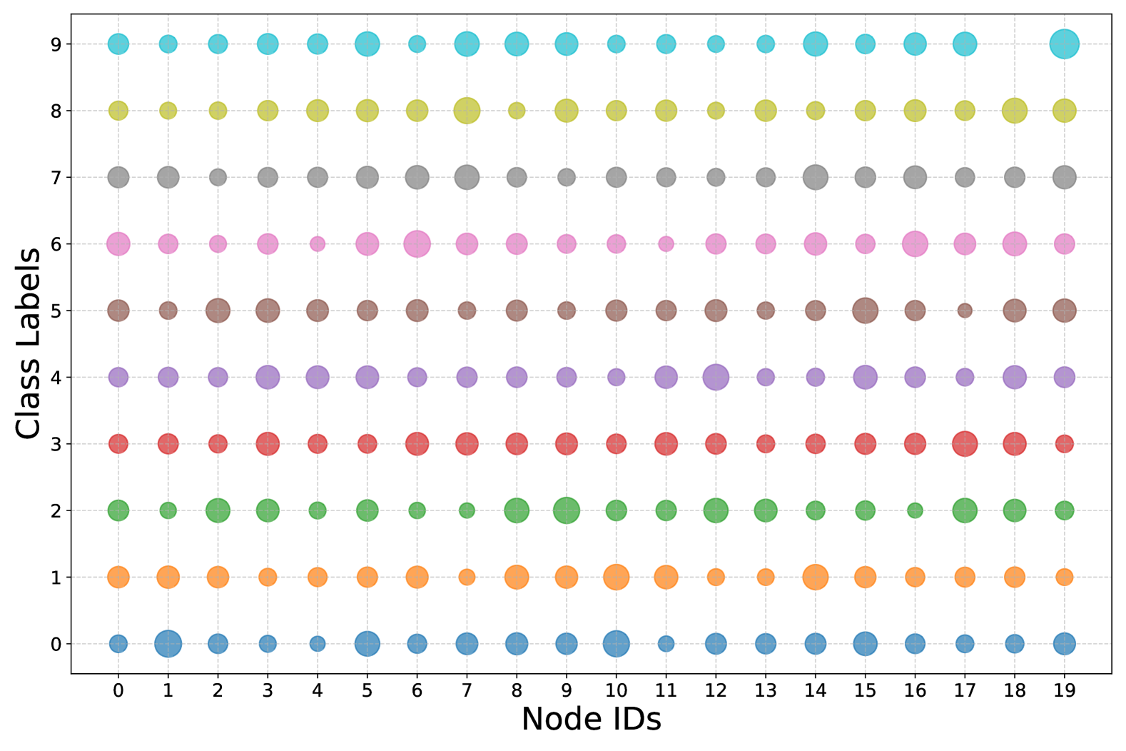
(a) $\alpha=10$.

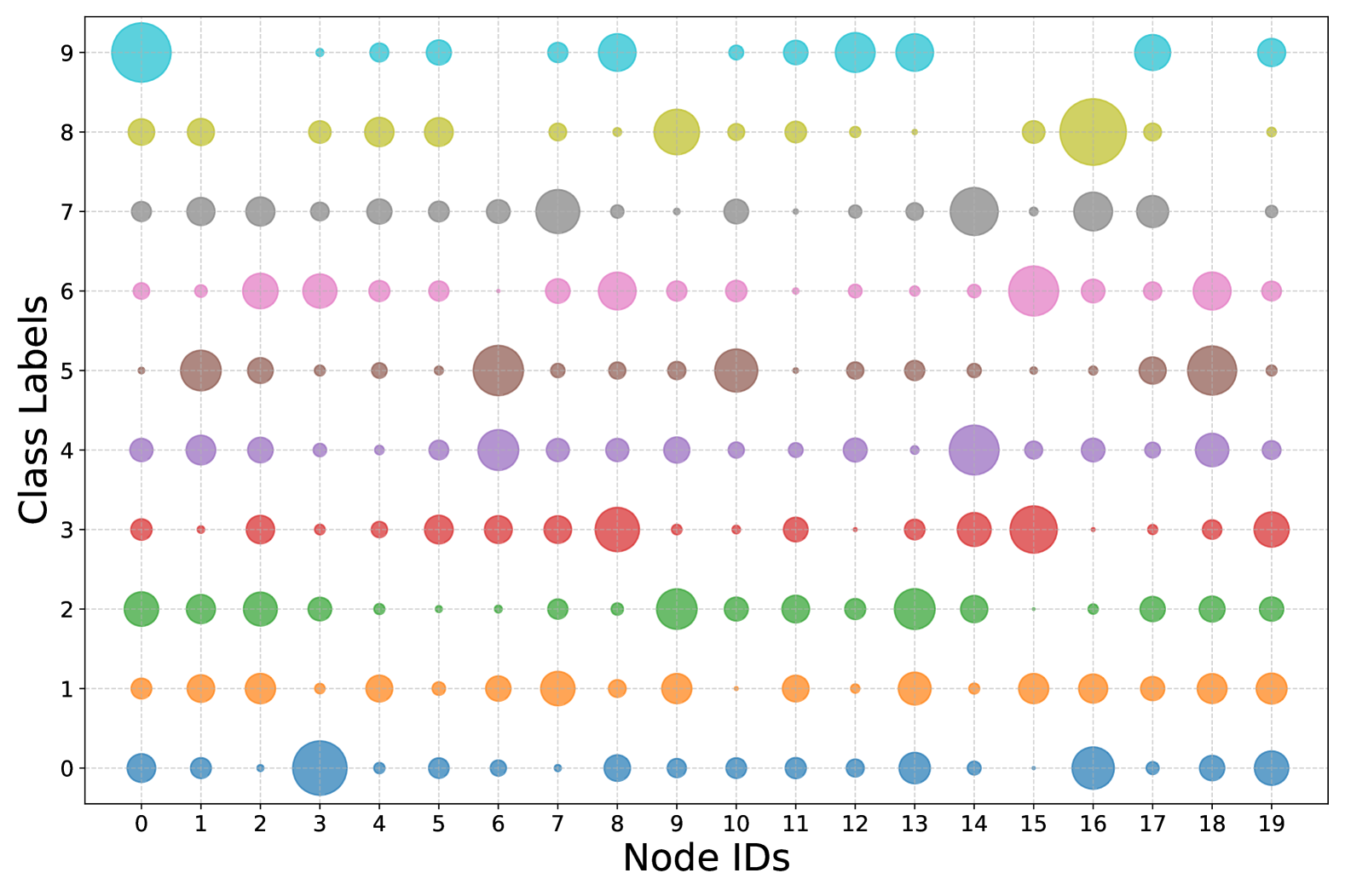
(b) $\alpha=1$.

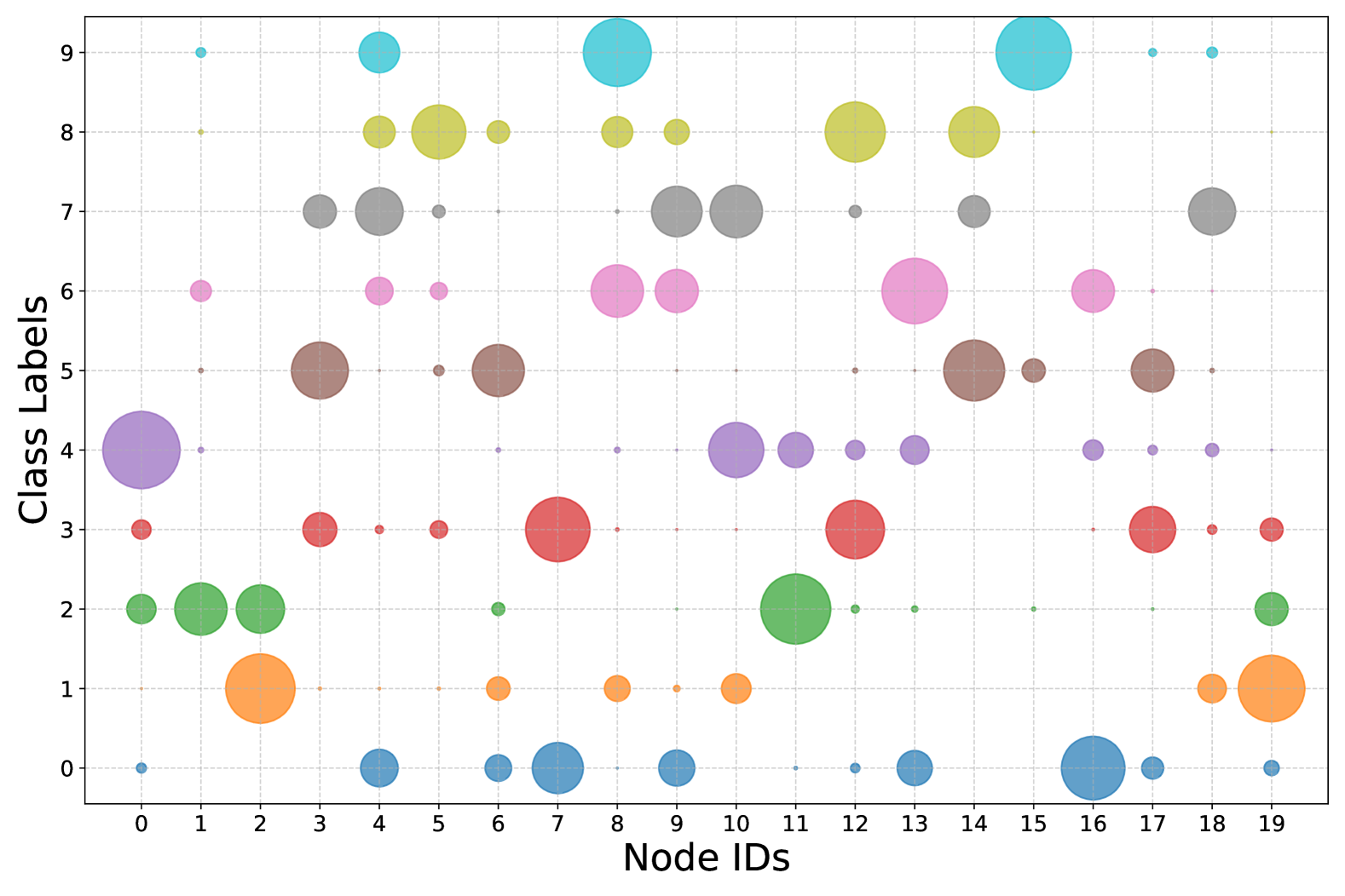
(c) $\alpha=0.1$.

Figure 5: Different levels of noniid-ness using Dirichlet distribution with different values of $\alpha$ for CIFAR-10.

E.2 Image Classification

The details are specified in Table 5.

Table 5: Default experimental settings for the image classification training

Dataset	CIFAR-$10$ (Krizhevsky, 2009)
Architecture	ResNet-$20$ (He et al., 2015)
Loss function	cross entropy
Accuracy objective	top-1 accuracy
Number of nodes	20
Topology	cycle, complete, Erdős–Rényi
Data distribution	iid (shuffled and split), non-iid (based on labels)
Local Steps $\tau$	5
Optimizer	SGD with momentum
Batch size	32 per client
Momentum	0.9 (Nesterov)
Initial learning rate	0.05
Learning rate schedule	multiplied by $0.1$ once after $75$ and once after $90$ percent of the training
Training time	$15$ minutes for $\alpha\in\{10,1\}$ and $30$ minutes for $\alpha=0.1$
Weight decay	$10^{-4}$
Learning rate warm-up time	$2$ minutes
Repetitions	10
Reported metric	mean and standard deviation of the aggregated model’s train loss and accuracy

E.3 Large Language Model Fine-tuning

The details are specified in Table 6.

Table 6: Default experimental settings for the large language model fine-tuning

Dataset	Multi- Genre Natural Language Inference (MultiNLI) corpus (Williams et al., 2018)
Architecture	OPT- $125$M (Zhang et al., 2022)
Loss function	cross entropy
Number of nodes	20
Topology	Erdős–Rényi
Data distribution	iid (shuffled and split), non-iid (based on genre)
Local Steps $\tau$	1
Optimizer	Adam
Batch size	16 sentences per client
Adam $\beta_{1}$	0.9
Adam $\beta_{2}$	0.999
Adam $\epsilon$	$10^{-8}$
Initial learning rate	$10^{-4}$
Learning rate schedule	multiplied by $0.1$ once after $75$ and once after $90$ percent of the training
Training time	$15$ minutes
Weight decay	$10^{-4}$
Learning rate warm-up time	$2$ minutes
Repetitions	10
Reported metric	mean and standard deviation of the aggregated model’s train loss

E.4 Experimental Network Topology

Figure 6 provides a schematic representation of the network topology and node distribution used in our experiments. The setup consists of 20 nodes grouped into 5 geographic clusters labeled CA, NV, IA, IL, and KS, each containing 4 nodes. Within each cluster, nodes are connected locally, while additional links enable communication across clusters, implementing decentralized computation and communication patterns.

We have conducted the experiments on the National Resource Platform (NRP) (San Diego Supercomputer Center, ) cluster. The 20 nodes used in our experiments are distributed across different physical machines located in multiple U.S. states. Most nodes are connected via high-speed research networks such as Science DMZs, with interconnect speeds ranging from 10G to 100G. This setup reflects a realistic decentralized learning environment over a wide-area network and introduces practical considerations like heterogeneous latency and bandwidth, which are difficult to model in simulation.

Figure 6: A 20-node decentralized system with 5 geographic clusters (CA, NV, IA, IL, KS).

Appendix F Extended Experiments

F.1 Analogy of Section 5.2 in a Cycle Topology

The goal of this section is to illustrate the analogy of Section 5.2 in a cycle topology. In the first row, Figures 7(a), 7(b), and 7(c) demonstrate the negative impact of increasing heterogeneity on the performance of both MW and Asynchronous Gossip. Here, in contrast to Section 5.2, we observe that both MW and Asynchronous Gossip degrade with a similar impact under extreme noniid conditions. However, MW continues to outperform Asynchronous Gossip. Notably, in small-diameter topologies such as Erdős–Rényi ($0.3$), the effect of extreme noniid conditions on MW is more severe than on Asynchronous Gossip. In Figure 7(i), we again observe that, in contrast to small-diameter topologies, MW continues to outperform even under extreme noniid conditions.

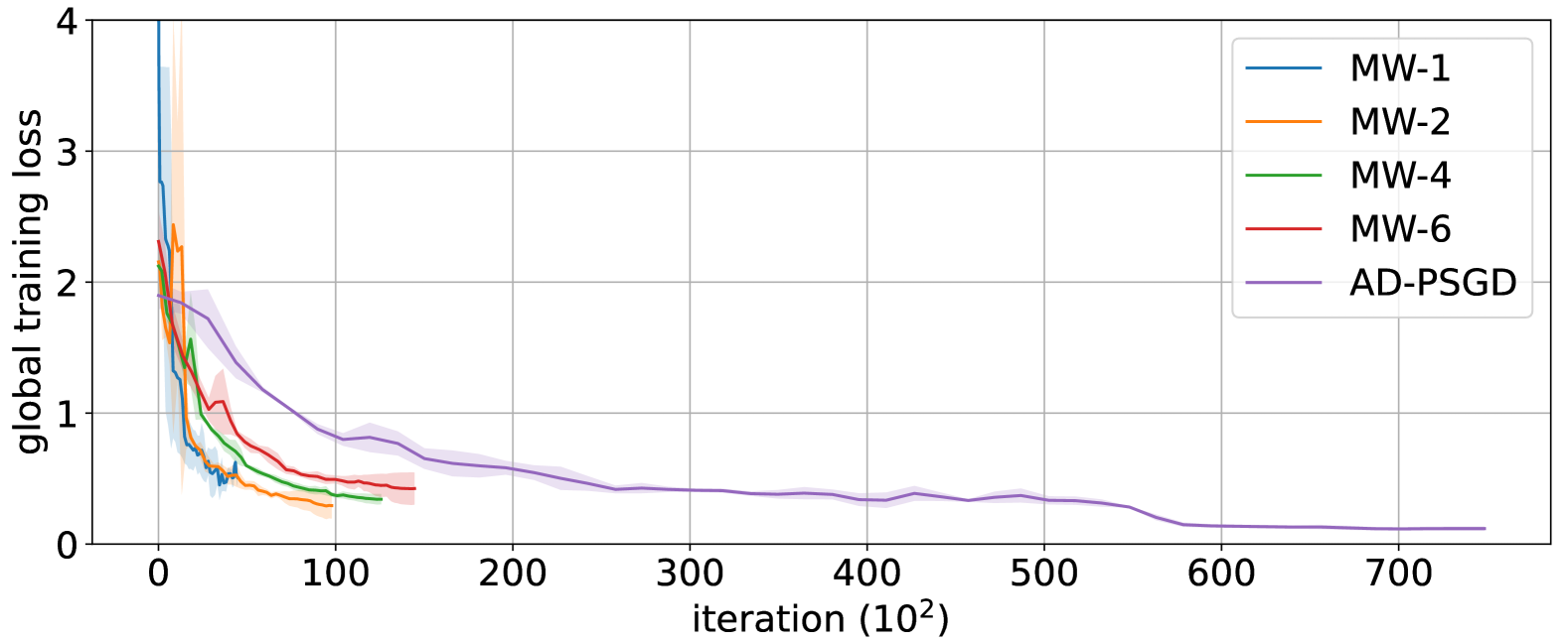
(a) $\alpha=10$, w.r.t iterations.

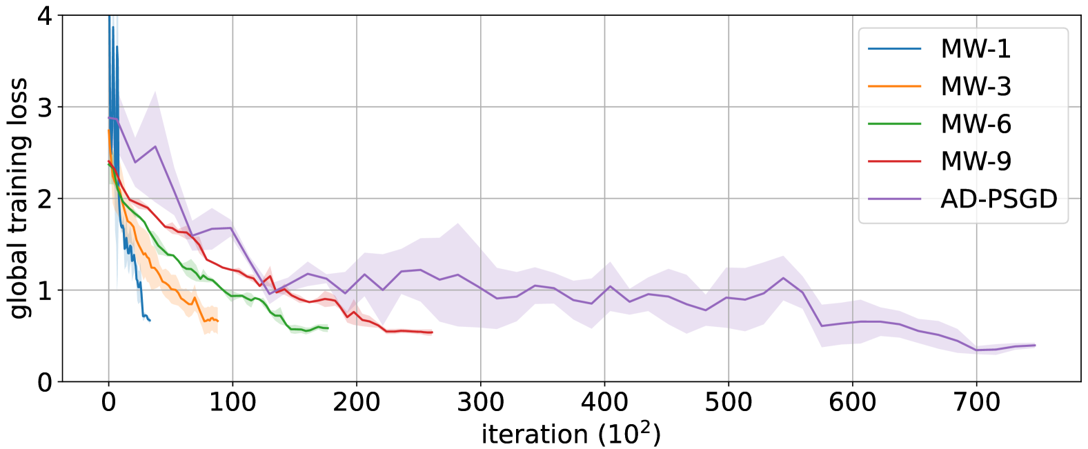
(b) $\alpha=1$, w.r.t iterations.

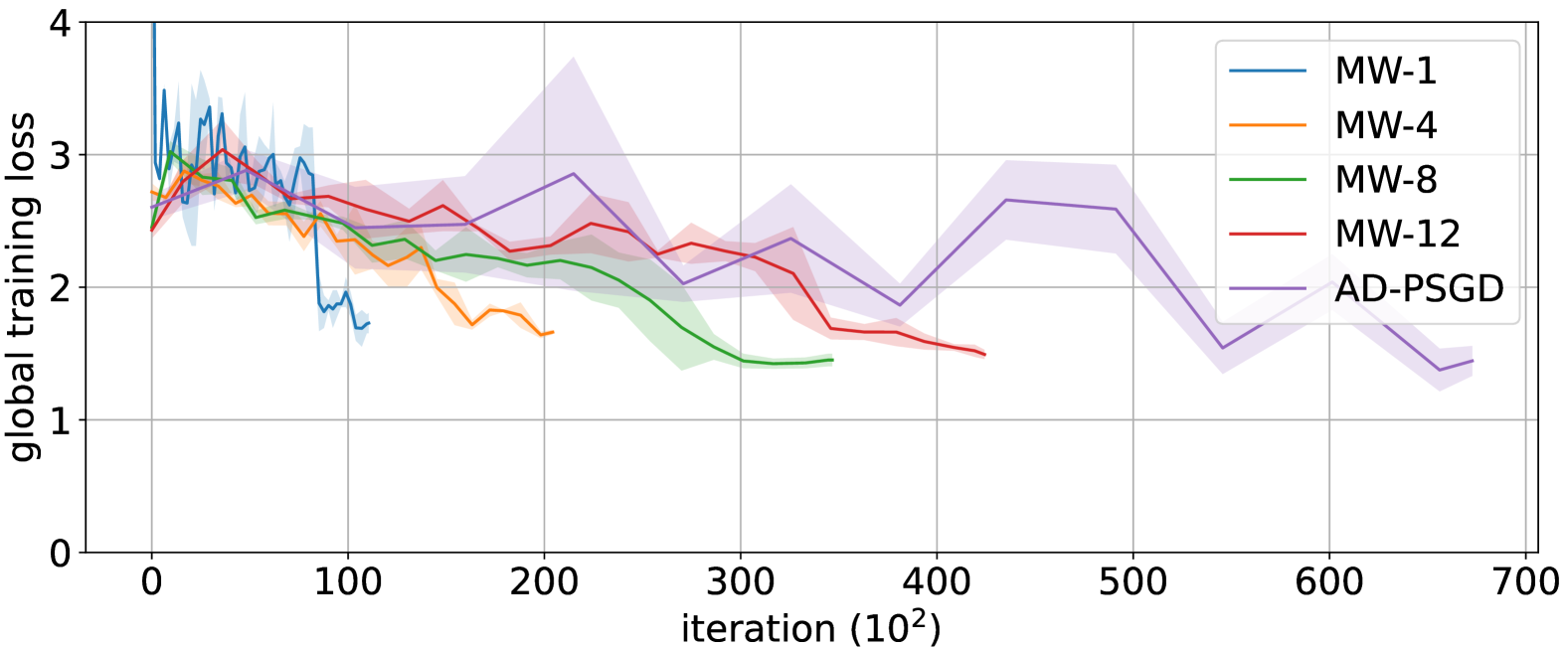
(c) $\alpha=0.1$, w.r.t iterations.

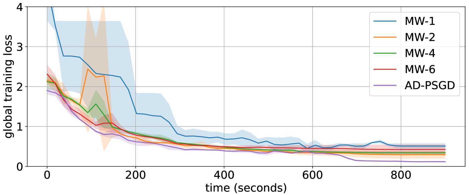
(d) $\alpha=10$, w.r.t wall-clock time.

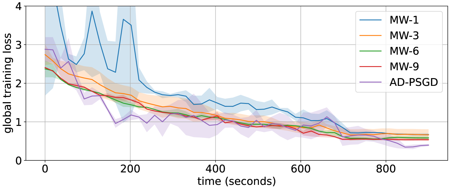
(e) $\alpha=1$, w.r.t wall-clock time.

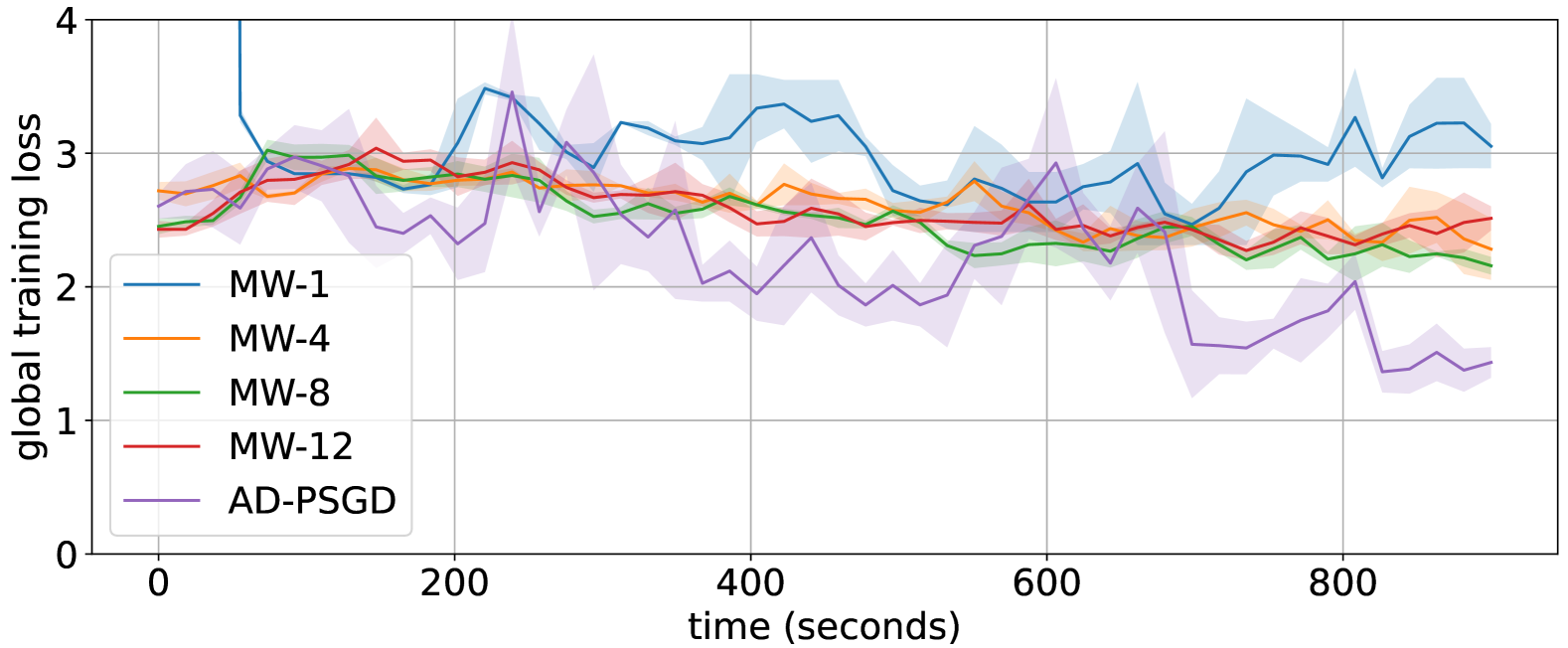
(f) $\alpha=0.1$, w.r.t wall-clock time.

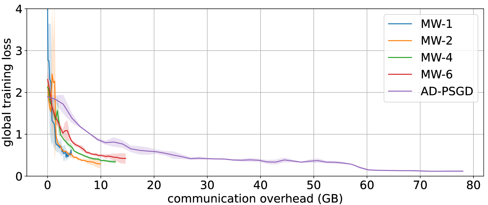
(g) $\alpha=10$, w.r.t transmitted bits.

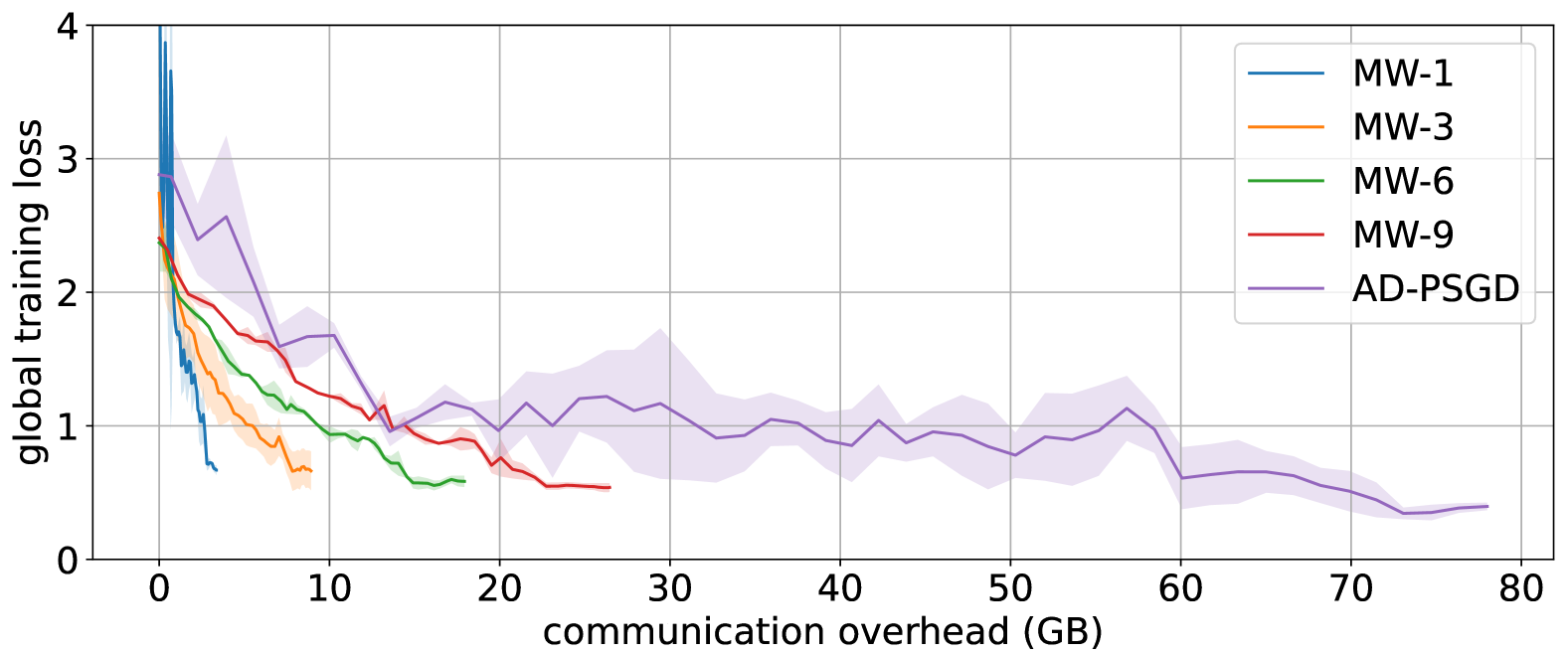
(h) $\alpha=1$, w.r.t transmitted bits.

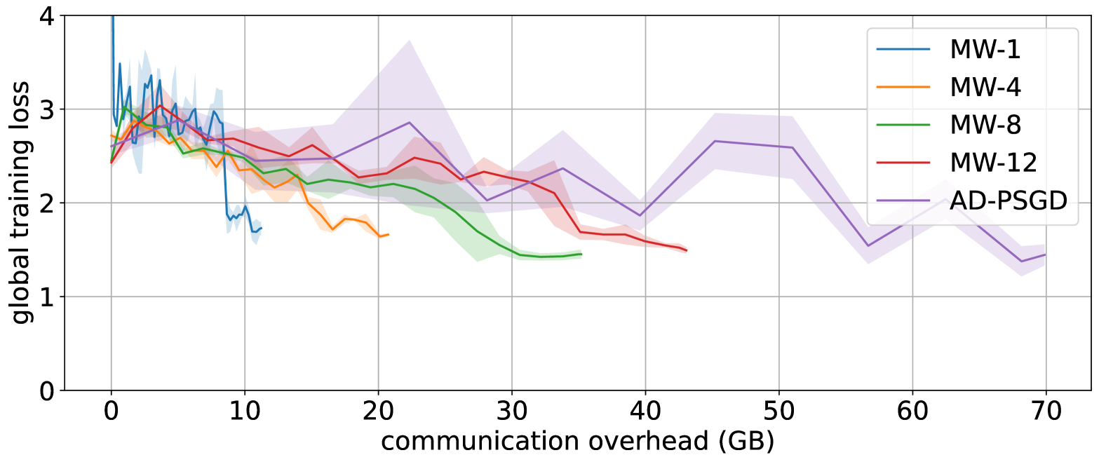
(i) $\alpha=0.1$, w.r.t transmitted bits.

Figure 7: Training of ResNet-$20$ on Cifar-$10$ on and $20$-node cycle network in different levels of noniid-ness.

F.2 Test Accuracy Performance of Section 5.2

In this subsection, we present the test accuracy results corresponding to the experimental setup described in Section 5.2. While the main paper focuses on analyzing the global training loss, here we provide a complementary view by reporting the test accuracy over the course of training. This offers further insight into the generalization performance of the models under varying conditions of data heterogeneity.

As with the loss-based analysis, we evaluate the test accuracy across multiple dimensions, w.r.t training iteration, wall-clock time, and communication cost (measured in transmitted bits). Across these different views, we observe consistent patterns in how data heterogeneity impacts convergence and accuracy. Specifically, the trends in test accuracy mirror those observed in training loss.

In addition to these metrics, we also report test accuracy w.r.t the number of epochs completed. This additional perspective allows us to assess how training progresses relative to the effective number of passes over the data. Note that the relationship between iteration and epoch is determined by the following formula:

$$\text{epoch}=\text{iteration}\times\tau\times\frac{\text{batch size}}{\text{size of the dataset}},$$ (137)

where $\tau$ denotes the number of local update steps performed by each client in a single iteration.

The results in Figure 8 provide a comprehensive view of how test accuracy evolves under while training ResNet-$20$ on Cifar-$10$ on and $20$-node Erdős–Rényi ($0.3$) graph for different levels of noniid-ness.

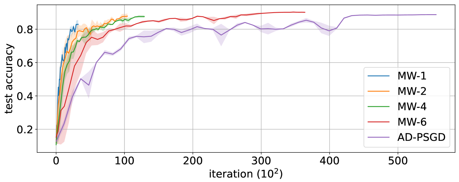
(a) $\alpha=10$, w.r.t iterations.

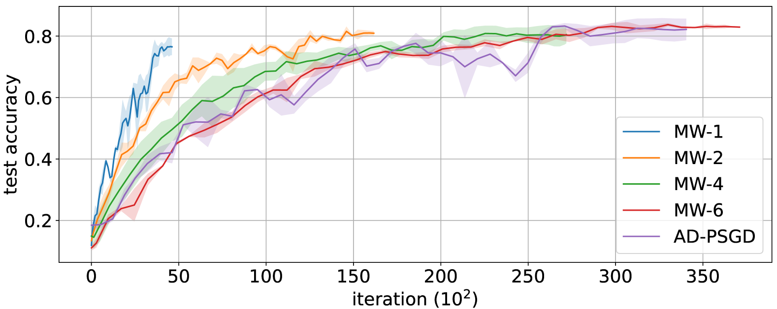
(b) $\alpha=1$, w.r.t iterations.

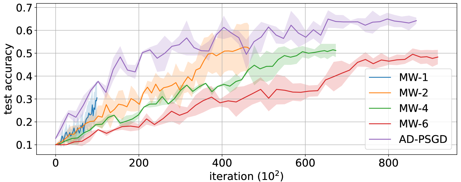
(c) $\alpha=0.1$, w.r.t iterations.

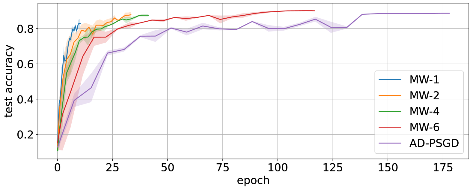
(d) $\alpha=10$, w.r.t epochs.

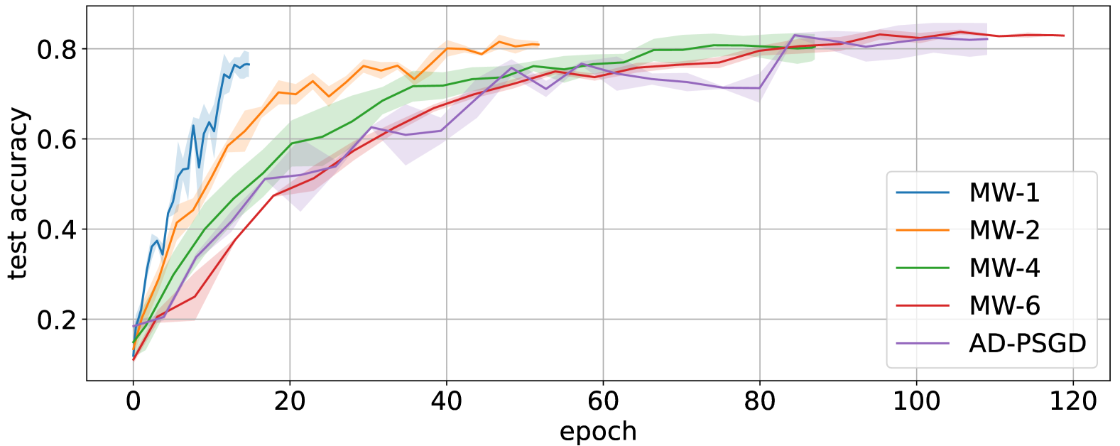
(e) $\alpha=1$, w.r.t epochs.

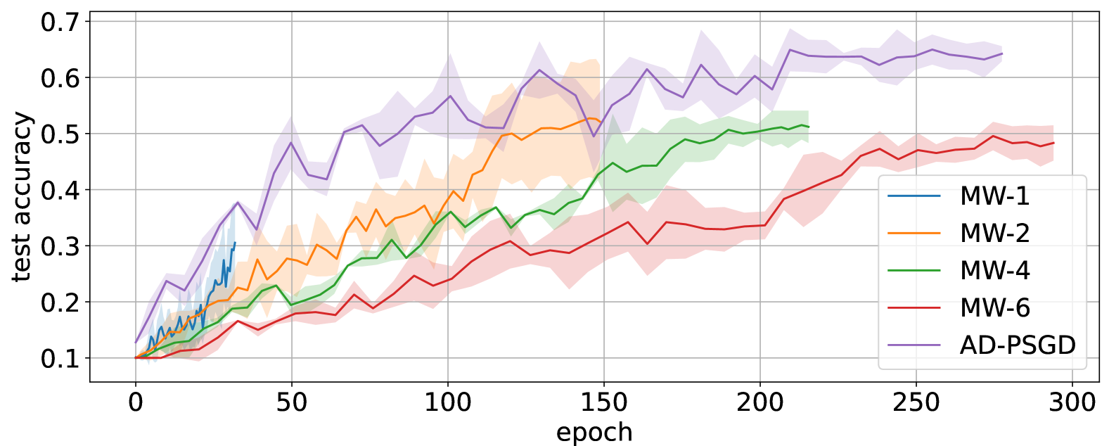
(f) $\alpha=0.1$, w.r.t epochs.

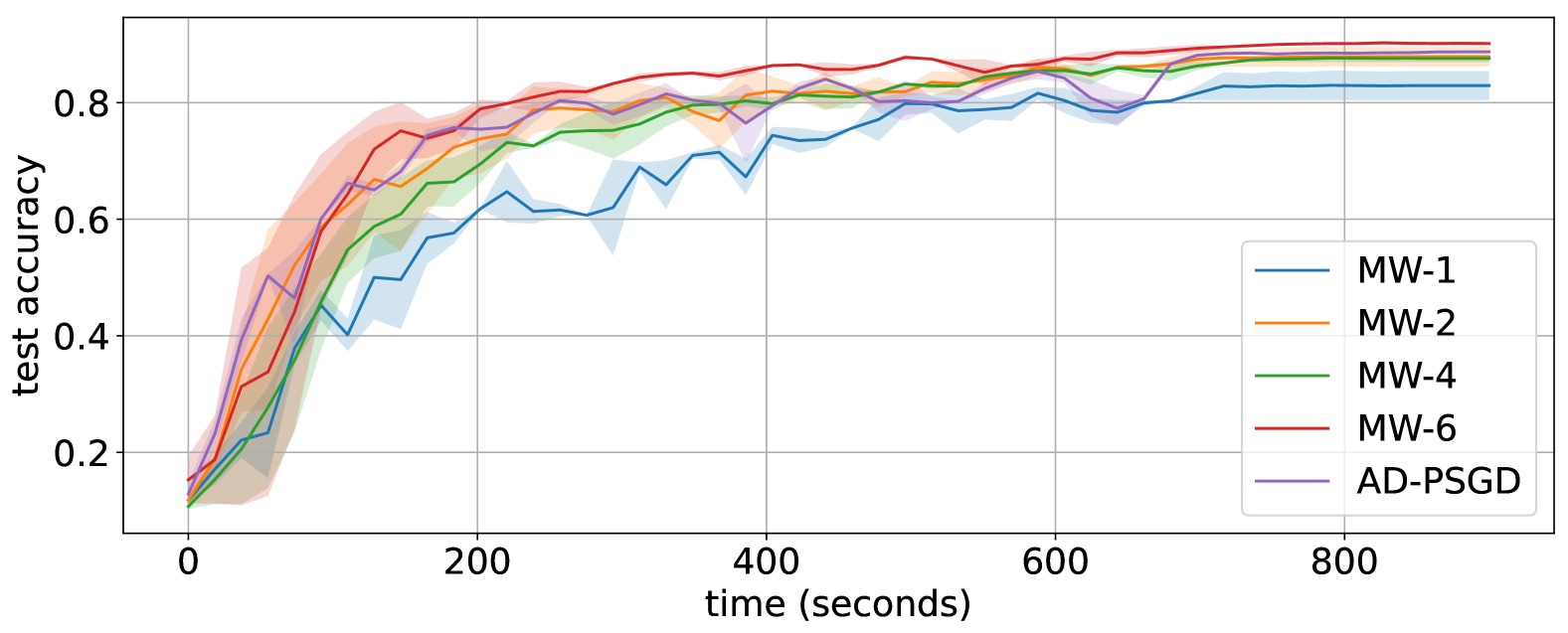
(g) $\alpha=10$, w.r.t wall-clock time.

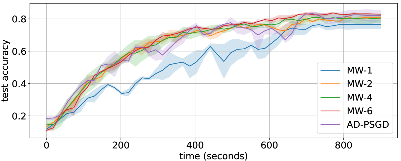
(h) $\alpha=1$, w.r.t wall-clock time.

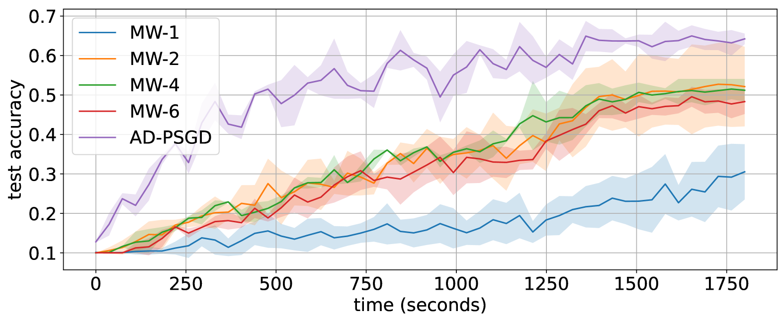
(i) $\alpha=0.1$, w.r.t wall-clock time.

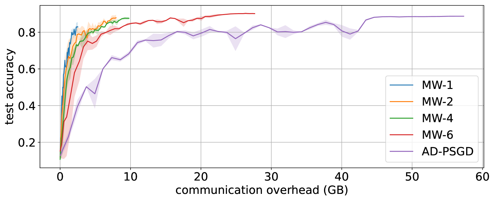
(j) $\alpha=10$, w.r.t transmitted bits.

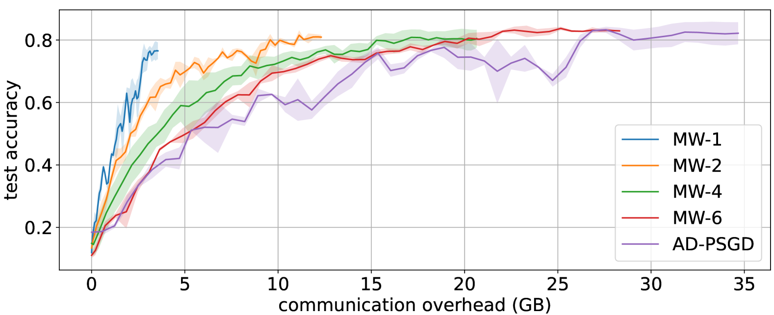
(k) $\alpha=1$, w.r.t transmitted bits.

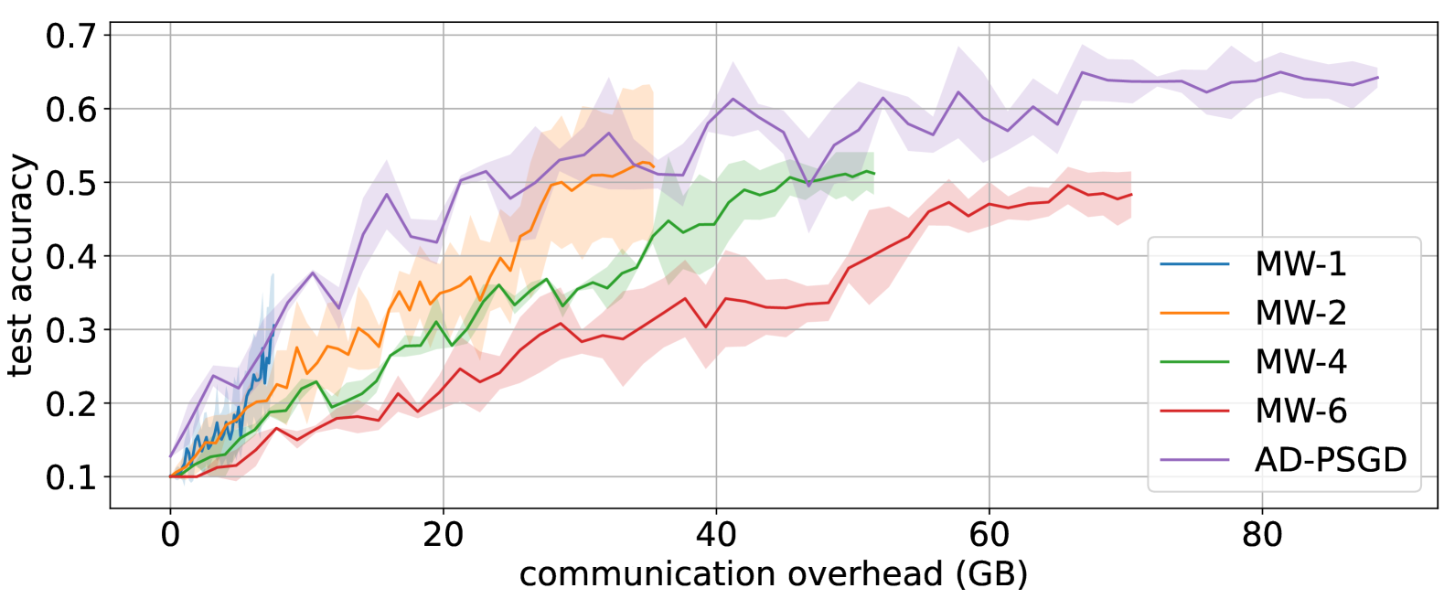
(l) $\alpha=0.1$, w.r.t transmitted bits.

Figure 8: Test accuracy of ResNet-$20$ on Cifar-$10$ on and $20$-node Erdős–Rényi ($0.3$) graph for different levels of noniid-ness.

References

- Agarwal & Duchi (2011) Agarwal, A. and Duchi, J. C. Distributed delayed stochastic optimization. 2012 IEEE 51st IEEE Conference on Decision and Control (CDC), pp. 5451–5452, 2011. URL https://api.semanticscholar.org/CorpusID:901118.
- Assran & Rabbat (2021) Assran, M. S. and Rabbat, M. G. Asynchronous gradient push. IEEE Transactions on Automatic Control, 66(1):168–183, January 2021. ISSN 2334-3303. doi: 10.1109/tac.2020.2981035. URL http://dx.doi.org/10.1109/TAC.2020.2981035.
- Ayache & Rouayheb (2020) Ayache, G. and Rouayheb, S. Y. E. Private weighted random walk stochastic gradient descent. IEEE Journal on Selected Areas in Information Theory, 2:452–463, 2020. URL https://api.semanticscholar.org/CorpusID:221651576.
- Baudet (1978) Baudet, G. M. Asynchronous iterative methods for multiprocessors. J. ACM, 25(2):226–244, April 1978. ISSN 0004-5411. doi: 10.1145/322063.322067. URL https://doi.org/10.1145/322063.322067.
- Bertsekas (1997) Bertsekas, D. A new class of incremental gradient methods for least squares problems. SIAM Journal on Optimization, 7(4):913–926, November 1997. ISSN 1052-6234. doi: 10.1137/S1052623495287022.
- Bornstein et al. (2022) Bornstein, M., Rabbani, T., Wang, E., Bedi, A. S., and Huang, F. Swift: Rapid decentralized federated learning via wait-free model communication, 2022. URL https://arxiv.org/abs/2210.14026.
- Bottou et al. (2018) Bottou, L., Curtis, F. E., and Nocedal, J. Optimization methods for large-scale machine learning, 2018. URL https://arxiv.org/abs/1606.04838.
- Boyd et al. (2006) Boyd, S. P., Ghosh, A., Prabhakar, B., and Shah, D. Randomized gossip algorithms. IEEE Transactions on Information Theory, 52:2508–2530, 2006. URL https://api.semanticscholar.org/CorpusID:2120244.
- Chen et al. (2017) Chen, J., Pan, X., Monga, R., Bengio, S., and Jozefowicz, R. Revisiting distributed synchronous sgd, 2017. URL https://arxiv.org/abs/1604.00981.
- Duchi et al. (2012) Duchi, J. C., Agarwal, A., and Wainwright, M. J. Dual averaging for distributed optimization: Convergence analysis and network scaling. IEEE Transactions on Automatic Control, 57(3):592–606, March 2012. ISSN 1558-2523. doi: 10.1109/tac.2011.2161027. URL http://dx.doi.org/10.1109/TAC.2011.2161027.
- Even et al. (2024) Even, M., Koloskova, A., and Massoulie, L. Asynchronous SGD on graphs: a unified framework for asynchronous decentralized and federated optimization. In Dasgupta, S., Mandt, S., and Li, Y. (eds.), Proceedings of The 27th International Conference on Artificial Intelligence and Statistics, volume 238 of Proceedings of Machine Learning Research, pp. 64–72. PMLR, 02–04 May 2024. URL https://proceedings.mlr.press/v238/even24a.html.
- Feyzmahdavian & Johansson (2021) Feyzmahdavian, H. R. and Johansson, M. Asynchronous iterations in optimization: New sequence results and sharper algorithmic guarantees. ArXiv, abs/2109.04522, 2021. URL https://api.semanticscholar.org/CorpusID:237485562.
- Gholami & Seferoglu (2024) Gholami, P. and Seferoglu, H. Digest: Fast and communication efficient decentralized learning with local updates. IEEE Transactions on Machine Learning in Communications and Networking, 2:1456–1474, 2024. doi: 10.1109/TMLCN.2024.3354236.
- Guruswami (2016) Guruswami, V. Rapidly mixing markov chains: A comparison of techniques (a survey), 2016. URL https://arxiv.org/abs/1603.01512.
- He et al. (2015) He, K., Zhang, X., Ren, S., and Sun, J. Deep residual learning for image recognition. 2016 IEEE Conference on Computer Vision and Pattern Recognition (CVPR), pp. 770–778, 2015.
- Kairouz et al. (2021) Kairouz, P., McMahan, H. B., Avent, B., Bellet, A., Bennis, M., Bhagoji, A. N., Bonawitz, K., Charles, Z., Cormode, G., Cummings, R., D’Oliveira, R. G. L., Eichner, H., Rouayheb, S. E., Evans, D., Gardner, J., Garrett, Z., Gascón, A., Ghazi, B., Gibbons, P. B., Gruteser, M., Harchaoui, Z., He, C., He, L., Huo, Z., Hutchinson, B., Hsu, J., Jaggi, M., Javidi, T., Joshi, G., Khodak, M., Konečný, J., Korolova, A., Koushanfar, F., Koyejo, S., Lepoint, T., Liu, Y., Mittal, P., Mohri, M., Nock, R., Özgür, A., Pagh, R., Raykova, M., Qi, H., Ramage, D., Raskar, R., Song, D., Song, W., Stich, S. U., Sun, Z., Suresh, A. T., Tramèr, F., Vepakomma, P., Wang, J., Xiong, L., Xu, Z., Yang, Q., Yu, F. X., Yu, H., and Zhao, S. Advances and open problems in federated learning, 2021. URL https://arxiv.org/abs/1912.04977.
- Koloskova et al. (2019) Koloskova, A., Stich, S., and Jaggi, M. Decentralized stochastic optimization and gossip algorithms with compressed communication. In Chaudhuri, K. and Salakhutdinov, R. (eds.), Proceedings of the 36th International Conference on Machine Learning, volume 97 of Proceedings of Machine Learning Research, pp. 3478–3487. PMLR, 09–15 Jun 2019. URL https://proceedings.mlr.press/v97/koloskova19a.html.
- Koloskova et al. (2020) Koloskova, A., Loizou, N., Boreiri, S., Jaggi, M., and Stich, S. A unified theory of decentralized SGD with changing topology and local updates. In III, H. D. and Singh, A. (eds.), Proceedings of the 37th International Conference on Machine Learning, volume 119 of Proceedings of Machine Learning Research, pp. 5381–5393. PMLR, 13–18 Jul 2020. URL https://proceedings.mlr.press/v119/koloskova20a.html.
- Koloskova et al. (2022) Koloskova, A., Stich, S. U., and Jaggi, M. Sharper convergence guarantees for asynchronous sgd for distributed and federated learning, 2022. URL https://arxiv.org/abs/2206.08307.
- Krizhevsky (2009) Krizhevsky, A. Learning multiple layers of features from tiny images. 2009.
- Levin & Peres (2017) Levin, D. A. and Peres, Y. Markov chains and mixing times: Second edition. 2017. URL https://api.semanticscholar.org/CorpusID:28640176.
- Lian et al. (2015) Lian, X., Huang, Y., Li, Y., and Liu, J. Asynchronous parallel stochastic gradient for nonconvex optimization. ArXiv, abs/1506.08272, 2015. URL https://api.semanticscholar.org/CorpusID:21782.
- Lian et al. (2017) Lian, X., Zhang, C., Zhang, H., Hsieh, C.-J., Zhang, W., and Liu, J. Can decentralized algorithms outperform centralized algorithms? a case study for decentralized parallel stochastic gradient descent. In Neural Information Processing Systems, 2017. URL https://api.semanticscholar.org/CorpusID:1467846.
- Lian et al. (2018) Lian, X., Zhang, W., Zhang, C., and Liu, J. Asynchronous decentralized parallel stochastic gradient descent, 2018. URL https://arxiv.org/abs/1710.06952.
- Lin et al. (2021) Lin, T., Karimireddy, S. P., Stich, S., and Jaggi, M. Quasi-global momentum: Accelerating decentralized deep learning on heterogeneous data. In Meila, M. and Zhang, T. (eds.), Proceedings of the 38th International Conference on Machine Learning, volume 139 of Proceedings of Machine Learning Research, pp. 6654–6665. PMLR, 18–24 Jul 2021. URL https://proceedings.mlr.press/v139/lin21c.html.
- McMahan et al. (2023) McMahan, H. B., Moore, E., Ramage, D., Hampson, S., and y Arcas, B. A. Communication-efficient learning of deep networks from decentralized data, 2023. URL https://arxiv.org/abs/1602.05629.
- Mishchenko et al. (2022) Mishchenko, K., Bach, F. R., Even, M., and Woodworth, B. E. Asynchronous sgd beats minibatch sgd under arbitrary delays. ArXiv, abs/2206.07638, 2022. URL https://api.semanticscholar.org/CorpusID:249674816.
- Nabli et al. (2023) Nabli, A., Belilovsky, E., and Oyallon, E. : Accelerating asynchronous communication in decentralized deep learning, 2023. URL https://arxiv.org/abs/2306.08289.
- Nadiradze et al. (2022) Nadiradze, G., Sabour, A., Davies, P., Li, S., and Alistarh, D. Asynchronous decentralized sgd with quantized and local updates, 2022. URL https://arxiv.org/abs/1910.12308.
- Nedić & Ozdaglar (2009) Nedić, A. and Ozdaglar, A. E. Distributed subgradient methods for multi-agent optimization. IEEE Transactions on Automatic Control, 54:48–61, 2009. URL https://api.semanticscholar.org/CorpusID:6489200.
- Needell et al. (2015) Needell, D., Srebro, N., and Ward, R. Stochastic gradient descent, weighted sampling, and the randomized kaczmarz algorithm, 2015. URL https://arxiv.org/abs/1310.5715.
- Recht et al. (2011) Recht, B., Ré, C., Wright, S. J., and Niu, F. Hogwild: A lock-free approach to parallelizing stochastic gradient descent. In Neural Information Processing Systems, 2011. URL https://api.semanticscholar.org/CorpusID:6108215.
- Robbins (1951) Robbins, H. E. A stochastic approximation method. Annals of Mathematical Statistics, 22:400–407, 1951. URL https://api.semanticscholar.org/CorpusID:16945044.
- (34) San Diego Supercomputer Center. National research platform (nrp) user guide. https://www.sdsc.edu/support/user_guides/nrp.html.
- Stich (2019) Stich, S. U. Local sgd converges fast and communicates little, 2019. URL https://arxiv.org/abs/1805.09767.
- Sun et al. (2018) Sun, T., Sun, Y., and Yin, W. On markov chain gradient descent. In Neural Information Processing Systems, 2018. URL https://api.semanticscholar.org/CorpusID:54074144.
- Tsitsiklis (1984) Tsitsiklis, J. N. Problems in decentralized decision making and computation. PhD thesis, Massachusetts Institute of Technology, 1984.
- Tsitsiklis et al. (1984) Tsitsiklis, J. N., Bertsekas, D. P., and Athans, M. Distributed asynchronous deterministic and stochastic gradient optimization algorithms. 1984 American Control Conference, pp. 484–489, 1984. URL https://api.semanticscholar.org/CorpusID:17975552.
- Williams et al. (2018) Williams, A., Nangia, N., and Bowman, S. A broad-coverage challenge corpus for sentence understanding through inference. In Proceedings of the 2018 Conference of the North American Chapter of the Association for Computational Linguistics: Human Language Technologies, Volume 1 (Long Papers), pp. 1112–1122. Association for Computational Linguistics, 2018. URL http://aclweb.org/anthology/N18-1101.
- Xiao & Boyd (2003) Xiao, L. and Boyd, S. P. Fast linear iterations for distributed averaging. 42nd IEEE International Conference on Decision and Control (IEEE Cat. No.03CH37475), 5:4997–5002 Vol.5, 2003. URL https://api.semanticscholar.org/CorpusID:6001203.
- Yuan et al. (2015) Yuan, K., Ling, Q., and Yin, W. On the convergence of decentralized gradient descent, 2015. URL https://arxiv.org/abs/1310.7063.
- Zhang et al. (2022) Zhang, S., Roller, S., Goyal, N., Artetxe, M., Chen, M., Chen, S., Dewan, C., Diab, M. T., Li, X., Lin, X. V., Mihaylov, T., Ott, M., Shleifer, S., Shuster, K., Simig, D., Koura, P. S., Sridhar, A., Wang, T., and Zettlemoyer, L. Opt: Open pre-trained transformer language models. ArXiv, abs/2205.01068, 2022. URL https://api.semanticscholar.org/CorpusID:248496292.
- Zheng et al. (2016) Zheng, S., Meng, Q., Wang, T., Chen, W., Yu, N., Ma, Z., and Liu, T.-Y. Asynchronous stochastic gradient descent with delay compensation. ArXiv, abs/1609.08326, 2016. URL https://api.semanticscholar.org/CorpusID:3713670.