Interference-caged quantum many-body scars: the Fock space topological localization and interference zeros

Abstract

We propose a general mechanism for realizing athermal finite-energy-density eigenstates—termed interference-caged quantum many-body scars (ICQMBS)—which originate from exact many-body destructive interference on the Fock space graph. These eigenstates are strictly localized to specific subsets of vertices, analogous to compact localized states in flat-band systems. Central to our framework is a connection between interference zeros and graph automorphisms, which classify vertices according to the graph’s local topology. This connection enables the construction of a new class of topological ICQMBS, whose robustness arises from the local topology of the Fock space graph rather than from conventional conservation laws or dynamical constraints. We demonstrate the effectiveness of this framework by developing a graph-theory-based search algorithm, which identifies ICQMBS in both a one-dimensional spin-1 XY model and two-dimensional quantum link models across distinct gauge sectors. In particular, we discover the proposed topological ICQMBS in the two-dimensional quantum link model and provide an intuitive explanation for previously observed order-by-disorder phenomena in Hilbert space. Our results reveal an unexpected synergy between graph theory, flat-band physics, and quantum many-body dynamics, offering new insights into the structure and stability of nonthermal eigenstates.

I Introduction

Understanding how information scrambles—and how to prevent it—poses a fundamental challenge in understanding correlated quantum many-body dynamics. The dynamics by which a generic closed quantum many-body system reaches a thermodynamic description after a long-time unitary evolution is referred to as thermalization. During the thermalization process, local operators scramble the information of a state, which is dissolved globally into the system. For a quantum ergodic system, one expects all initial states to thermalize [1, 2, 3, 4]. i.e., any initial state within a narrow energy density shell will equilibrate to a state that acts as a thermal reservoir for its own subsystems. Thus, arbitrary subsystems of these states are described by the same ensemble theory, making them thermodynamically indistinguishable by local observables.

Despite the intuitive appeal of quantum ergodicity, rigorously proving its validity for general systems remains an open challenge. A major breakthrough came with the development of the eigenstate thermalization hypothesis (ETH) [5, 6], which provides a mathematically concrete ansatz of a thermal state based on statistical behavior and quantum chaos. Due to its strong predictive power, ETH has since been validated through both numerical [7, 8] and experimental studies [9, 10, 11] and has been widely regarded as a universal description for eigenstates at finite energy density.

An intriguing question is whether there are mechanisms that can violate ETH and, if so, how these violations occur. Systems with strong ergodicity breaking, like integrable systems or those with many-body localization (MBL) [12, 13], have extensively many conserved quantities that prevent all eigenstates from being thermal. However, due to the subtle interpretation of numerical evidence from finite-size systems, MBL’s stability is still under debate [14, 15, 16].

In contrast to strong ergodicity breaking, weak ergodicity breaking systems, where only a small subset of eigenstates violate ETH, were initially considered rare and irrelevant. However, experiments with Rydberg atom quantum simulators revealed persistent long-time coherent oscillations for certain initial states [17]. These unexpectedly long-lived oscillations suggest an anomalous resilience of the quantum state against thermalization. Such non-thermal eigenstates, dubbed as quantum many-body scars (QMBS) [18, 19], draw an analogy to the well-known quantum scars observed in single-particle chaotic systems [20, 21, 22]. In addition to QMBS, it was later found that a more general phenomenon could emerge in correlated dynamics where the Hilbert space is fragmented [23, 24, 25, 26] into dynamically disconnected blocks. The anomalous dynamics of QMBS and Hilbert space fragmentation are beyond the conventional symmetry analysis and have sparked interest due to their fundamental implications [27, 28, 29, 30] and potential applications [31, 32, 33].

The anomalous dynamical behavior of QMBS is closely related to the constraints induced by Rydberg blockade in the experiment [34, 35, 17, 18]. The discovery of QMBS and Hilbert space fragmentation also sparked the investigation of the physics for constrained systems with strong local interactions [36, 37, 38, 39, 40, 41, 42], with novel fractonic dynamics dictated by dipole conservation [43, 44, 45], in frustrated magnets [46] and with gauge structure [47, 48, 49, 50, 51, 52, 53, 54, 55, 56, 57, 58, 59, 60, 61, 62, 63, 64, 65]. Recent advancements in two-dimensional quantum simulator experiments have further demonstrated the possibilities of studying nontrivial dynamics of such 2D systems with local constraints [66, 40, 67]. Both theoretical and experimental discoveries on QMBS and Hilbert space fragmentation urge a general understanding of how a decoupled subspace can emerge within the many-body Hilbert space beyond conventional symmetry reasoning.

One general approach to understanding these phenomena is to start from the Hilbert space and operator algebras associated with higher symmetries. These include methods such as the spectrum-generating algebra (SGA) [68, 69], group-invariant sectors [70, 71, 72], and quasisymmetry groups [73, 74]. Although their specific constructions differ, these approaches share a common principle: by exploiting the algebraic structure of higher symmetries, one can devise symmetry-breaking operators with arbitrary weights to eliminate the targeted non-thermal states. In general, such operators give rise to a non-integrable Hamiltonian while still preventing coupling between thermal and targeted non-thermal states. Following these approaches, even though the resulting Hamiltonian lacks explicit information about higher symmetries, the underlying algebraic structure of higher symmetry still dictates the decoupling between thermal and non-thermal states. Physically, these approaches are closely related to the algebraic description of stable quasi-particles for specific vacuum states and have received significant successes in explaining QMBS in several iconic models, including the spin-1 XY chain [75], $\eta$-paring in Hubbard models [76, 77, 78, 69], and Affleck-Kennedy-Lieb-Tasaki (AKLT) model [79, 80, 81]. However, its strong attachment to the quasi-particle picture also raises an intriguing question of whether the quasi-particle picture is necessary for understanding non-thermal eigenstates.

Another approach considers the problem of the projector embedding method proposed by Shiraishi and Mori [82]. This method decouples Hilbert space into thermal and embedded non-thermal subspaces using local projectors. By leveraging this structure, eigenstates satisfying the conditions set by local projectors can be explicitly embedded into the spectrum, as seen in systems exhibiting topological order [83, 84] and lattice supersymmetry [85]. Recently, it has also been shown that the projector embedding approach can be applied to the PXP model [86] and demonstrated the non-trivial connection between the embedding approach and the gauge structure [87]. However, while the projector embedding framework provides a mathematically general construction, it does not impose constraints on the physical origin of the underlying algebraic structure. As a result, the stability of the embedded states depends crucially on the physical origin of the local projectors, making this an inherently non-trivial problem [83].

In the stable quasi-particle approaches, the decoupling between non-thermal and thermal states relies on the implicit algebraic structure dictated by higher symmetries, even though the final Hamiltonian does not explicitly preserve these symmetries. In the projector embedding approach, the decoupling is achieved by designing the neat local structure of the Hamiltonian. These two frameworks represent fundamental mechanisms to decouple the non-thermal many-body quantum states, eliminating the coupling by crafting the Hamiltonian using symmetry protection and local projectors. The unification of the two approaches in several models has also been discussed recently [87]. Even though the two frameworks describe QMBS in many models and shed much light on the mathematical structure that hosts them, addressing the reverse question from the first principle is still challenging.

In addition to the above-mentioned mechanisms, destructive interference of quasi-particles has also been identified as a key factor in certain types of QMBS [75]. However, compared with the previous two mechanisms, it is relatively less studied. In $S=1$ XY model [75], QMBS exhibit two distinct forms of quasi-particle interference: (a) Frustration-free QMBS, arising from bimagnon interference, can be understood within the frameworks of Shiraishi-Mori’s projector embedding scheme and the SGA approach. (b) Non-frustration-free QMBS, involving bond-bimagnon interference, currently lacks a well-defined description within the projector embedding or SGA framework, to the best of our knowledge. This distinction suggests that quasi-particle interference may serve as a fundamental physical mechanism for QMBS, with some states falling within the scope of projector embedding and SGA approaches while others remain beyond these descriptions. Given this, it is tempting to promote the relatively unexplored interference structure as the origin of QMBS. However, several crucial open questions remain for these interference-induced QMBS, as noted in the supplementary material of [75]: Can the analysis of quasi-particle interference be generalized beyond one-dimensional systems? Can we go beyond the quasi-particle picture to understand QMBS? If such a generalization is established, what would be the algebraic description of these QMBS? Can we systematically identify such states or detect them through some numerical or experimental phenomena?

The essence of this work lies in proposing the many-body destructive interference as a general and physical mechanism for the emergence of a decoupled non-thermal subspace within the many-body Hilbert space. We refer to this class of QMBS as interference-caged quantum many-body scars (ICQMBS). The idea of ICQMBS extends the idea of strictly localized wavefunctions from the single-particle Hilbert space, where their robustness arises from local topology [88, 89, 90, 91], to the many-body Hilbert space using the Fock space graph. Rather than requiring a flat many-body spectrum in quantum numbers, we investigate these emergent non-thermal states through the entanglement patterns induced by interference and the vanishing fluctuation of corresponding local operators. Unlike the prior mentioned mechanisms, which depend on explicit algebraic structures, ICQMBS emerges from an intrinsic physical interference mechanism. Building on this framework, we devise an algebraic description and the corresponding algorithm to analyze ICQMBS. The interference mechanism provides a flexible and comprehensive framework for QMBS, that is independent of system dimensionality, the stability of the quasi-particle picture, or the frustration-free condition.

The notion of ICQMBS reveals the unforeseen robustness of real-space local perturbation respecting the hidden topological structure of the quantum many-body system. We dubbed such ICQMBS as topological ICQMBS(tICQMBS). The non-trivial robustness against real-space perturbation triggered the analysis from the Fock space graph point of view, and we found the state is robust against any perturbation that kept the Fock space interference pattern intact. i.e., the perturbation could break translation symmetry, time-reversal symmetry or even the hermicity. The absolute robustness of the topological ICQMBS provides another angle to understand the effects of the disorder beyond the projector embedding approach [82] or the intricate Onsager symmetry construction [93]. Furthermore, ICQMBS also provides a natural explanation of the order-by-disorder in the Hilbert space(OBDHS) phenomena [56] in two-dimensional constrained systems where the origin of QMBS is relatively unexplored.

This paper is organized as follows:

• Sec. II provides a foundational review of the Fock space graph representation, beginning with a brief introduction to relevant graph theory terminology. We then discuss the choice of the basis used to define fictitious particles on a well-defined Fock space graph and compare this approach to the standard tight-binding model. Through these discussions, we illustrate how locality is encoded within the Fock space graph representation.

• Sec. III introduces the concept of ICQMBS. We begin with a simple time-reversal and translationally invariant Hamiltonian, explaining how interference patterns lead to localized subgraphs, which form the basis of ICQMBS. This intuitive framework serves as a stepping stone for the formal description of ICQMBS developed in later sections. Based on this insight, we introduce an algorithmic approach to identifying ICQMBS using Fock space graph structure and explore the role of graph automorphisms in their identification.

• Sec. IV builds on the intuition developed in Sec. III to provide a more formal characterization of ICQMBS. The key structure underlying ICQMBS is the pattern of interference zeros in the Fock space, which governs the non-thermal nature of the eigenstates. We further analyze the relationship between interference zeros and the topological properties of ICQMBS. For tICQMBS, we present a formal procedure to embed these states into the spectrum and construct the corresponding Hamiltonian. This construction explicitly demonstrates the robustness of tICQMBS and highlights their existence beyond conventional symmetry-based analyses.

• Sec. V applies the theoretical framework to a concrete example—the one-dimensional spin-1 XY model, which has been extensively studied in previous works [75, 30]. Due to its simplicity, this model provides a clear and intuitive demonstration of our approach and serves as an example of emergent ICQMBS.

• Sec. VI extends our analysis to non-trivial two-dimensional lattice gauge theory (LGT) models with local constraints, focusing on the $U(1)$ QLM and QDM. Notably, QDM can be interpreted as a $U(1)$ QLM in a different gauge sector. After introducing these models, we review key numerical results from prior studies on QMBS [56, 94, 57] and apply our framework to analyze their structure. We explicitly demonstrate the interference patterns responsible for Type-I and IIIA QMBS and explain the anomalous OBDHS effect in terms of Fock space topological localization, where robustness is a direct consequence of local topology. This analysis provides a concrete example of tICQMBS.

• Sec. VII concludes the paper with a discussion of several open questions on ICQMBS and related challenges in fully understanding the mechanisms underlying QMBS.

II Graph representation of a quantum many-body system

The Fock space graph representation has been widely used in various studies, including investigations of quantum ergodicity and localization in high-dimensional Fermi systems with large molecules [95, 96], disordered quantum dots [97], MBL [98], and early explorations of one-dimensional QMBS [18]. Related ideas have also been applied in the study of fragmentation [99], quantum complexity in many-body problems [100], and slow dynamics in quantum East model [101]. In Sec. II.1, we first consider time-reversal symmetric Hamiltonians, where the Fock space graphs are weighted by real values. We then address the more complicated case in which the graph edges carry complex weights. In Sec. II.2, we clarify the subtle differences between quasi-particles and the fictitious particles defined within the Fock space graph—a representation that inherently depends on the choice of basis. Since the basis selection is closely tied to the symmetry of Hamiltonian, we provide the physically motivated arguments for choosing a suitable basis that is compatible with the symmetries of a generic system. In Sec. II.3, we then examine the subtle differences between standard tight-binding models and Fock space graphs.

Readers may find the use of Fock space graphs to analyze translationally invariant interacting quantum many-body systems unnecessary or even overly complicated, given that the resulting graph often features correlated onsite disorder and intricate connectivity. The advantages of this approach will become clear once we introduce the concept of Fock space topological localization and the corresponding analysis in Sec. III and Sec. IV.

II.1 The Fock space graphs and graph terminologies

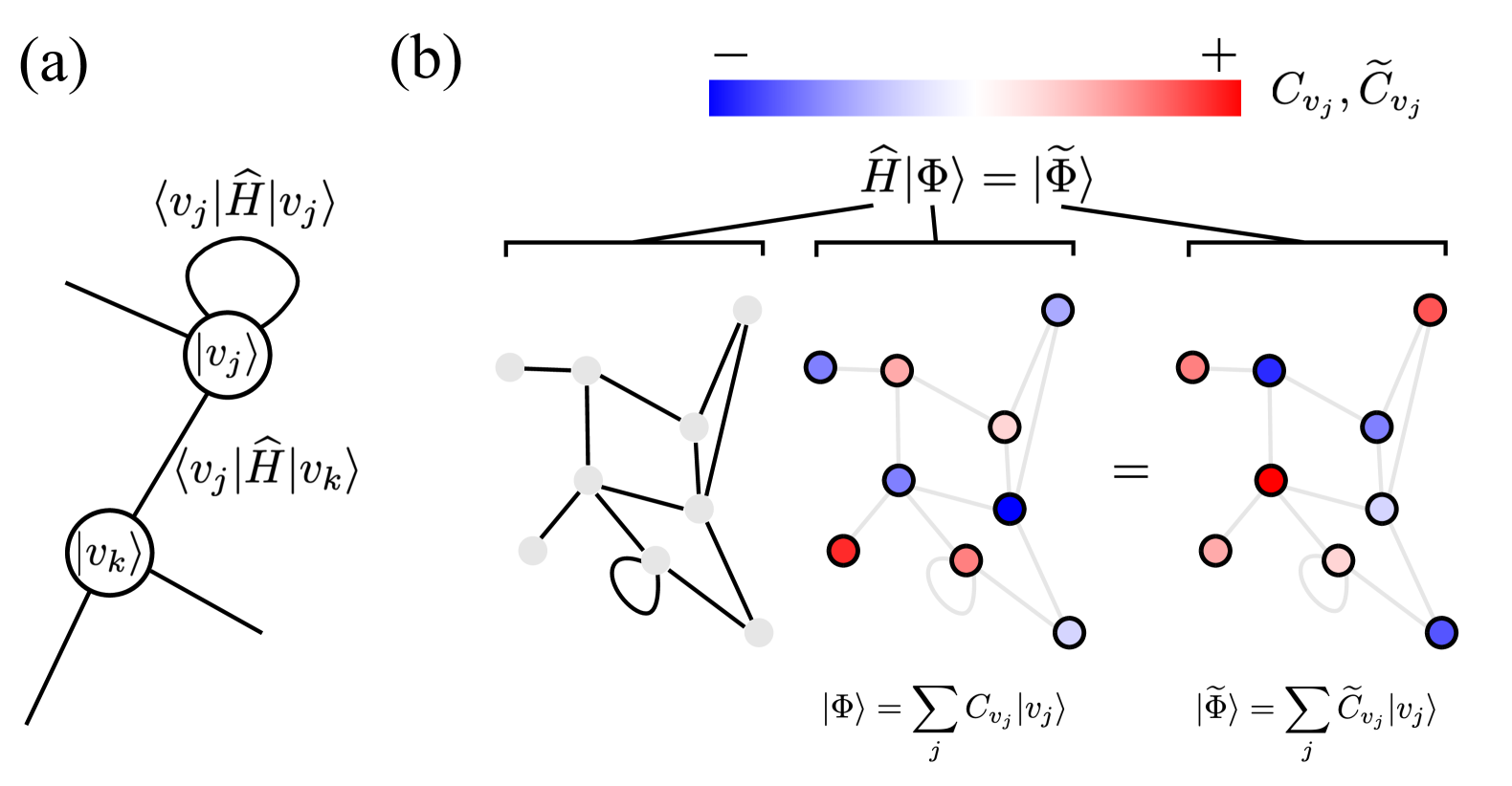
Figure 1: Schematic of the Fock space graph: (a) Each vertex represents a general many-body basis state $|v_{j}\rangle$ in the Fock space. For example, $|v_{j}\rangle$ can represent a spin configuration basis $|\uparrow\uparrow\downarrow\cdots\rangle$, or an occupation number basis $|021\cdots\rangle$, depending on the system. The edges connecting vertices represent the Hamiltonian matrix element between two states, and the self-loops attached to each vertex correspond to the diagonal terms. Here, we focus on the Hamiltonian with real-valued representation, resulting in a graph with undirected edges (no arrows). (b) The plot shows how a Hamiltonian applies to a many-body state. The vertex colors represent the real-valued weights $C_{v_{j}}$ and $\widetilde{C}_{v_{j}}$, without the overall normalization. The weights of the state $|\Psi\rangle$ are redistributed into $|\widetilde{\Psi}\rangle$ according to the Hamiltonian.

The Fock space graph, or Fock space lattice, is a general description of a quantum many-body system governed by Hamiltonian dynamics. In such a system, the Fock space $\mathcal{F}$ represents the space where the system’s instantaneous states are defined, while the Hamiltonian operator $\widehat{H}$ dictates the unitary time evolution. Here, we assume the locality of $\widehat{H}$ according to the tensor product structure of the many-body Hilbert space. The most common situation is the real-space local Hamiltonian, where the many-body Hilbert space of system $\Omega$ is formed by $\mathcal{H}_{\Omega}=\bigotimes_{\mathbf{r}\in\Omega}\mathcal{H}_{\mathbf{r}}$ with dimension $N_{\mathcal{F}}$. The information of the Fock space and the Hamiltonian can be encoded in a graph, consisting of a set of vertices $V$ and edges $E$, which connect them as shown in Fig. 1. The vertices, $v_{j}\in V$, represent the basis $|v_{j}\rangle\in\mathcal{H}_{\Omega}$. The edges connecting the vertices $v_{j}$ and $v_{k}$, denoted by the ordered pairs $e\left(v_{j},v_{k}\right)\in E$, carry weights given by the complex matrix elements $\langle v_{j}|\widehat{H}|v_{k}\rangle$. In general, these edges are directed when the matrix elements are complex, leading to $\langle v_{j}|\widehat{H}|v_{k}\rangle\neq\langle v_{j}|\widehat{H}|v_{k}\rangle$. For constrained Hilbert space, the constraints remove the direct product structure of the Hilbert space $\mathcal{H}_{\Omega}$. The modification is to isolate the constraint-violating vertices in the Fock space graph, which simply means a different graph structure. The Fock space graph, therefore, has the advantage of treating correlated quantum dynamics of many-body systems with or without constraints on equal footing.

For simplicity, we first focus on the homogeneous, time-reversal symmetry Hamiltonians and basis choices such that the matrix elements of the Hamiltonians are real . The corresponding graph is formed by undirected edges, weighted by the Hamiltonian’s matrix elements, as illustrated in Fig. 1 (a). In this graph representation, the diagonal terms correspond to self-loops attached to each vertex, while the off-diagonal terms represent edges connecting different vertices. The off-diagonal tunneling between basis states $|v_{j}\rangle$ and $|v_{k}\rangle$ is governed by uniform local operators in real space, with the corresponding energy scale set to $1$. The diagonal terms of the Hamiltonian are described by dimensionless energy scales $\left\{U_{i}\right\}$. Specifically, the Hamiltonian in this study can be cast into the following form:

$$\widehat{H}=\sum_{j,k=1}^{N_{\mathcal{F}}}A_{v_{j},v_{k}}|v_{j}\rangle\langle v_{k}| =\widehat{O}_{\text{kin}}+\widehat{O}_{\text{pot}}(\left\{U_{i}\right\})$$ (1)

$$\widehat{O}_{\text{kin}} =\sum_{j,k=1\atop j\neq k}^{N_{\mathcal{F}}}A_{v_{j},v_{k}}|v_{j}\rangle\langle v_{k}|$$

$$\widehat{O}_{\text{pot}}(\left\{U_{i}\right\}) =\sum_{j=1}^{N_{\mathcal{F}}}A_{v_{j},v_{j}}|v_{j}\rangle\langle v_{j}|\text{.}$$

We are in general interested in systems with non-trivial dynamics, where $\left[\widehat{O}_{\text{kin}},\widehat{O}_{\text{pot}}(\left\{U_{i}\right\})\right]\neq 0$. The adjacency matrix $A$ is a matrix representation of the Fock space graph, with $A_{v_{j},v_{k}}$ representing the off-diagonal matrix elements, which are zero unless the state $|v_{j}\rangle$ can couple to $|v_{k}\rangle$ through $\widehat{O}_{\text{kin}}$. The diagonal elements $A_{v_{j},v_{j}}$ depend on the details of $|v_{j}\rangle$ and the energy scales $\left\{U_{i}\right\}$. The $\widehat{O}_{\text{kin}}$ term mimics the particle-like hopping from $v_{j}$ to $v_{k}$ on the Fock space graph, while the $\widehat{O}_{\text{pot}}(\left\{U_{i}\right\})$ term mimics the on-site potential. To make later discussion concrete and to avoid confusion with the quasi-particle notion, we use the term fictitious particle hopping to describe the particle-like hopping on Fock space graphs in later discussions. Moreover, since the graph visually represents the Hamiltonian, we may occasionally use the terms Hamiltonian $\widehat{H}$, adjacency matrix $A$, and graph $G$ interchangeably.

The power of this representation rests on its generality. Any Hamiltonian can be represented as a graph. Likewise, any quantum state at time $t$, $|\psi(t)\rangle$, can be described in terms of weighted vertices as follows:

$$|\psi(t)\rangle=\sum_{j=1}^{N_{\mathcal{F}}}C_{v_{j}}(t)|v_{j}\rangle\text{,}$$ (2)

with $\sum_{j=1}^{N_{\mathcal{F}}}|C_{v_{j}}(t)|^{2}=1$. This representation is not limited by the dimensionality of the system, and the locality of the Hamiltonian is reflected in the sparsity of the graph.

At first glance, the Fock space graph may appear to simply rephrase the original problem, with its structure depending on the choice of basis. However, it provides additional insights. First, without explicitly specifying the correspondence between the vertices with the physical basis state, the Fock space graph itself does not uniquely represent a physical system. Instead, it represents a family of quantum systems where the many-body states of different systems are coupled in the same fashion, as discussed in the caption of Fig. 1 (a). Therefore, the Fock space graph serves as an abstraction of quantum many-body dynamics. This abstraction can be interpreted as the most strict version of the universality class for quantum Hamiltonian dynamics. Second, the relationships between states are made explicit in the Fock space graph representation. While the full Hamiltonian matrix implicitly contains information about how states are coupled, the Fock space graph shows explicitly how many steps are required to couple one basis state to another, as illustrated in Fig. 1 (b). The second property is important for identifying the interference patterns, which we will discuss in later sections.

II.2 The choice of basis for the Fock space graphs

The Fock space graph serves as a general, basis-dependent representation. With insights from the Fock space graph, can we argue a suitable choice of basis to develop a general understanding of QMBS, to devise efficient algorithms for finding QMBS, and to explain unknown phenomena? Before addressing these key questions, we will explore the proper choice of basis and related considerations in the study of QMBS in Sec. II.2.1. In particular, we need to discuss how symmetries are considered in this context. With a fixed basis, or equivalently, a fixed graph structure, the fictitious particle becomes well-defined. The clear distinction between quasi-particles and fictitious particles will be discussed in Sec. II.2.2, the latter of which plays a major role in Fock space topological localization introduced in Sec. III.

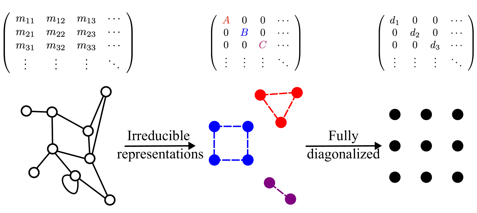
Figure 2: Schematic diagram of ED procedure using the Fock space graph representation. (Left) The initial product state basis is represented by blank circles. (Middle) The block-diagonalized Hamiltonian, formed by irreducible basis states, is represented by disconnected graphs, with the new basis shown as red, blue, and purple circles. (Right) Once the system is fully diagonalized, the Fock space graph is formed by isolated vertices, represented by black circles. The colored circles are, in general, entangled states.

II.2.1 Symmetries and the choice of basis

The physical definition of QMBS, as non-thermal quantum many-body eigenstates, is a basis-independent property. However, the notion of fictitious particles is inherently basis-dependent. Hence, what is the appropriate choice of basis for identifying QMBS from the perspective of thermalization? In addition, the choice of basis is closely related to the symmetries of the system. How do symmetries enter our analysis when investigating the origin of QMBS? With these questions in mind, we will first discuss the subtle role that symmetries play in the search for QMBS. Then, we will discuss the scheme for selecting a suitable basis and its relation with the sub-volume law entanglement entropy observed in QMBS.

To get exact information on excited many-body states, we usually rely on exact diagonalization (ED). During the implementation of ED, one typically begins by analyzing the system’s symmetries. By collecting states transformed according to the irreducible representations of the symmetry group $\mathcal{G}$, the Hamiltonian can be block-diagonalized. In the study of thermalization, constructing the block-diagonalized Hamiltonian is important for two reasons. First, it allows us to investigate whether there is a non-trivial mechanism that violates ETH, which assumes the components of the wave functions are independent. By block diagonalizing, we can avoid situations where some states are orthogonal purely due to trivial symmetries. Second, decoupling the Hamiltonian into smaller blocks reduces the matrix size, making it feasible to perform ED on each block individually. Given computation resources, we can extract more information to understand the thermodynamic limit. In terms of the Fock space graph, block diagonalizing the Hamiltonian is equivalent to disentangling the connected graph into smaller, connected components through unitary transformations. Further diagonalizing these smaller pieces of connected graphs corresponds to disentangling all the graphs into isolated vertices, as shown in Fig. 2.

From the perspective of searching QMBS, the conventional ED procedure seems relatively detoured since the sub-volume law entanglement entropy condition is not incorporated, neither when we block diagonalize the Hamiltonian based on the system’s symmetries, $\mathcal{G}$, nor when we diagonalize the smaller blocks after the unitary transformation. After fully diagonalizing the Hamiltonian, we then calculate the bipartite entanglement entropy for exponentially many eigenstates, looking for the ones that exhibit the sub-volume law entanglement. While using symmetry reduces the computational cost and allows us to study larger system sizes, it also obscures the mechanism that leads to sub-volume law entanglement in mid-gap eigenstates.

Instead of following the conventional ED procedure, we devise our analysis procedure targeting QMBS’s anomalous entanglement property. To start our analysis, we choose the basis states, represented by vertices in the graph, with minimum entanglement. Specifically, in our search for QMBS, we start with real-space product states, which have zero bipartite entanglement entropy, as the basis for the graph representation.

Nevertheless, we can still take advantage of certain symmetries in our system. Specifically, we focus on symmetries that enable block diagonalization of the Hamiltonian directly within the product state basis. These states can be used to analyze the interference pattern due to the fictitious particle. For example, in QLM or QDM, we only block diagonalize the Hamiltonian based on sectors labeled by local charges and electric fluxes. While translation and rotational symmetries exist, we avoid using them to block diagonalize the Hamiltonian, as doing so requires basis transformations, e.g., Fourier transformations, that mix product states. Such transformations typically involve the summation of bases that alter the graph topology and obscure the destructive interference, a key mechanism for realizing QMBS, as we will discuss in section III It is also worth noting that lattice point-group symmetries are not completely ignored. Instead, they manifest as part of the graph automorphisms, a key mathematical structure that will be discussed in Sec. III.3 .

In summary, we start the discussion from the $N_{\mathcal{F}}\times N_{\mathcal{F}}$ many-body Hamiltonian $\widehat{H}$, which can be interpreted as an adjacency matrix $A$ defining an undirected, weighted graph $G=\{V,E\}$. The choice of basis for the graph is based on the entanglement properties of the basis states. We aim to block diagonalize the Hamiltonian as much as possible while keeping the basis as product states. The graph may contain self-loops but forbids both multiple edges and multiple loops. In this framework, the vertex set $V$ represents the many-body basis, with each vertex corresponding to a product state on the computational basis. The edges $e\left(v_{j},v_{k}\right)\in E$ connect vertices $v_{j}$ and $v_{k}$, with weights given by the off-diagonal matrix element $A_{v_{j},v_{k}}$. The graph is considered connected, ensuring a path exists between every pair of vertices, which implies the system does not break quantum ergodicity trivially. The number of edges attached to a vertex is referred to as the vertex’s degree, and self-loops can appear on each vertex $v_{j}$ if the diagonal matrix element $A_{v_{j},v_{j}}$ is present .

II.2.2 The fictitious particles and the quasi-particles

The fictitious particle is a basis-dependent description and is not equivalent to the quasi-particles, which have measurable properties. The fictitious particle is a mathematical device to understand how the weight of the wave function is transferred from one vertex to another in the Fock space according to the Hamiltonian, as shown in Fig. 1 (b). On the other hand, quasi-particle is a notion that characterizes a many-body excitation relative to a particular ground state, with long lifetimes, behaving like a particle. Quasi-particles can carry both extrinsic physical observable, such as momentum, and intrinsic physical degrees of freedom, such as spin and charge.

In unconstrained models, e.g., the spin-1 XY chain that we will discuss later, the fictitious particle hopping can be interpreted as quasi-particles [75]. In these cases, the fictitious particle naturally associates with a particle-like excitation on the lattice that can move freely, without kinetic constraints, within the corresponding parameter regime. In constrained models, such as the two-dimensional QLM [103, 104] or QDM [105] on a square lattice that we will discuss later, identifying the fictitious particle with the quasi-particle might be less natural. In these cases, the fictitious particle hopping on the Fock space graph is restricted by dynamical constraints between product states, such as those imposed by the Gauss law in QLM and QDM. The nature of quasi-particle excitations varies dramatically across different parameter regions of the model.

For example, for QDM on a square lattice (the only dimensionless energy scale $U_{1}\coloneqq\lambda$ in Eq. (29)), quasi-particle excitations are generally formed by the superpositions of dimer coverings, where the role of dynamical constraint is smeared. In the ideal columnar phase (with the kinetic energy term tuned to $-\infty$, or equivalently $\lambda=0$), the fictitious particle can roughly be identified with the quasi-particle, as the weight of ground state wave function is concentrated on the maximally flippable state. However, as we move into the parameter region where $\lambda$ is finite but small ($0<\lambda\ll 1$), the weight is redistributed into different dimer coverings, making the identification of the fictitious particle with the quasi-particle increasingly less meaningful as $\lambda\to 1^{-}$. This distinction becomes most dramatic at $\lambda=1$, where the model becomes exact-solvable. When the model is at the frustration-free Rokhsar-Kivelson point, $\lambda=1$, the ground state is formed by an equal-weight superposition of all possible dimer coverings, and the quasi-particle excitation here becomes considerably different from the fictitious particle. Instead, these excitations are described by the resonons [106], spinless and charge neutral quasi-particles that have attracted intensive research due to their connection with correlated superconductivity [107, 108] and spin liquids [105].

II.3 Tight-binding model on the real space lattice and on the Fock space graph

Before delving into the key mechanism that leads to QMBS, it is important to make a distinction between the tight-binding model and the Fock space graph. Given the similarities in hopping and on-site potentials between the two, it may be tempting to view the Fock space graph as a straightforward generalization of the standard tight-binding model. However, we want to emphasize several subtle differences between the two.

First, the on-site potentials in the Fock space graph are highly correlated, as the hopping is induced by local operators, meaning that $|v_{j}\rangle$ and $|v_{k}\rangle$ only differ locally. This property adds another layer of complexity to the problem because the disorder potential defined on the graph is correlated .

Second, since the Fock space graph is not defined in real space, it lacks crystalline symmetry. The key structure of the Fock space graph lies in how the vertices are connected, which is dictated by whether two many-body states can be coupled through a translationally invariant Hamiltonian. To start our discussion, we focus on the simplest non-trivial model and disregard the weights on the edges. In that sense, the property of the Fock space graph that concerns us most is its topology .

Guided by the abovementioned properties, the objective becomes clear: What is a generic topological mechanism that can localize eigenstates on a Fock space graph while lacking crystalline symmetry? At first glance, the Fock space graph is convenient for understanding the origin of QMBS from an entanglement perspective. However, identifying a universal mechanism to localize eigenstates on such a complex graph appears elusive. Even if such a mechanism exists, it is challenging to identify QMBS due to the complexity of the graph. Furthermore, can this generic mechanism shed new light on unexplained phenomena in the study of QMBS? Remarkably, we found that combining two seemingly unrelated research territories—flat-band physics and graph automorphisms—overcomes these obstacles and provides a neat explanation of the OBDHS mechanism for QMBS [56]. We will discuss flat-band physics and graph automorphisms in the following sections.

III Interference-caged quantum many-body scars–intuition

In this section, we discuss the mechanism and the algorithm to identify the interference-caged quantum many-body scars. In Sec. III.1, we will give a brief review on the topological localization emphasizing the robustness established on the local topology instead of the crystalline symmetry. Therefore, the idea can be generalized easily to the Fock space graph with complex topology. Once the notion of Fock space topological localization is well defined, we can formulate the interference-caging condition in its most general form in Sec. III.2. From the geometric meaning of the interference-caging condition, we propose to formulate the search problem into a constrained combinatorial analysis based on the graph automorphism in Sec. III.3. We will start with simple but efficient conditions, to understand the nature of the problem. Inspired by this simple but instructive approach, we develop a graph automorphism-based observations to identify the interference pattern. We will discuss the bipartite Fock space graph in Sec. III.3.3, which simplifies the search for interference patterns significantly. At the end of this section, we will discuss some guiding principles for finding interference patterns based on the graph automorphism approach and elaborate on the obstacles we encountered when discussing the problem in its most general settings.

After we introduce the general framework and the origin of ICQMBS, we will study specific examples in Sec. V and Sec. VI. To keep the generality of our approach, we benchmark our results with ED in the two sections discussing a one-dimensional system without dynamical constraints and two-dimensional systems with different gauge constraints respectively.

To the best of our knowledge, the underlying mechanism of the ICQMBS is fundamentally different from the currently proposed unified formalisms. The idea of ICQMBS starts from the physical assumptions, instead of the algebraic properties, about the QMBS. Therefore, the precise connection between ICQMBS and other unification schemes is an intriguing open question for future studies.

III.1 Topological localization and the Fock space topological localization

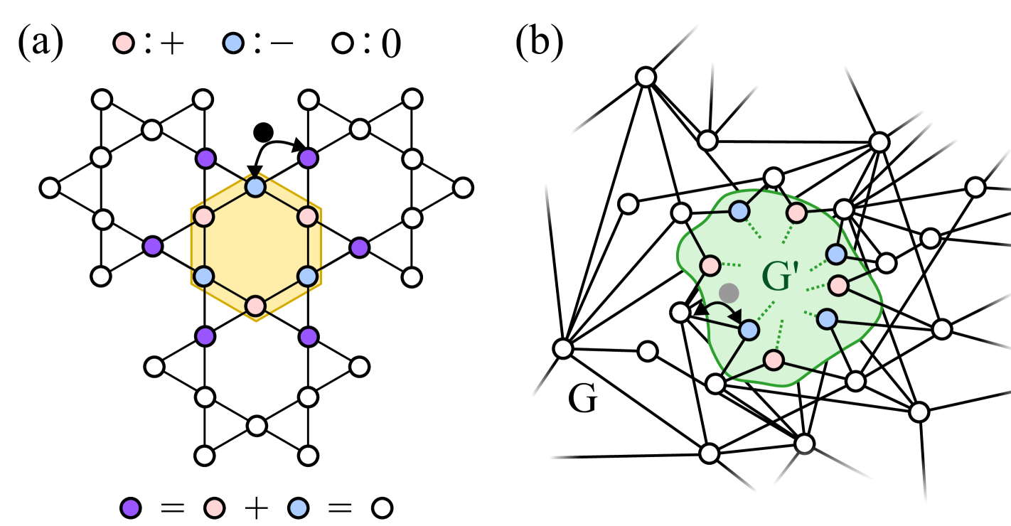
Figure 3: Topological localization in real space with quasi-particle picture and in the Fock space with fictitious particle picture: (a) The Kagome lattice tight-binding model. A quasi-particle (a black circle) can hop on the Kagome lattice. The interference happened at the boundary sites (purple circles) with mixed red and blue wights that cancel each other. (b) The schematic Fock space graph, $G$, for the Hamiltonian (1). To avoid cluttering the picture and emphasize the similarity with the tight-binding model in (a), we omit the self-loops in the figure and only draw the off-diagonal part of the adjacency matrix. A fictitious particle (grey circle) can hop between vertex $v_{j}$ to vertex $v_{k}$. We found the many-body version of the destructive interference pattern for the fictitious particle contributes to the formation of QMBS. The interference pattern for QMBS divides the vertices into two parts. One with non-zero weights on the vertices, the induced subgraph $G^{\prime}$, and the other with zero weights.

The lack of energy scale for the dispersionless band makes the flat-band systems dominated by the interaction term. The setting, therefore, becomes a Cornucopia for non-trivial correlated emergent phenomena. There is a long history of the study of flat-band physics in a wide variety of contexts. A detailed discussion of the flat-band physics is beyond the scope of this work . Recent experiment advances on kagome metals and moirè systems also motivate further investigation for novel mechanisms to the flat band physics [114, 115] and make the flat band physics an active and interdisciplinary research area.

We will focus on the strictly localized states [88, 90] or the compact localized states [89, 91] for flat-bands and its generalization to the Fock space. The strictly localized states were first discussed on the dice lattice [88]. The bipartiteness induced destructive interference led to localized orbits which have support on a diminishing fraction of the system as the system approaches the thermodynamic limit. Such a localized state can coexist with the itinerant states and can, in principle, appear at any energy in the band gap or within the continuum. The state remains robust unless the local interference pattern is broken. Therefore, the localized state is also considered to be localized due to the local topology of the system and can exist even when the lattice periodicity is destroyed or in different dimensions. The simplest non-trivial example to demonstrate the physics is the tight-binding model defined on the geometrically frustrated Kagome lattice (See Fig. 3 (a)). The tight-binding Hamiltonian on the Kagome lattice is

$$\widehat{H}^{Kagome}_{TB}=-t\sum_{\langle j,k\rangle}c^{\dagger}_{j}c_{k}+h.c.\text{.}$$ (3)

Here, lattice sites $j,k$ are on the Kagome lattice with hopping amplitude $-t$. The simplest compact localized state is shown in Fig. 3 (a) with a yellow plaquette. The localized wave function is constructed by equal weight superposition of the vertices basis with alternative signs. The general structure of the localized wave functions is the destructive interference of fictitious-particle (in this non-interacting case, equivalent to a quasi-particle) hopping at its boundary and leading to the dispersionless band. One can discuss the robustness of the localized state by considering the perturbation to the tight-binding model. As long as the local interference pattern is not altered by the perturbation, the eigenstate will remain localized. The origin of the localized state is not due to the symmetry. Instead, it is due to the local topology [88], the structure that dictates how sites are connected locally such that destructive interference is possible. Inherited from the topological localization in real space, the Fock space topological localization also does not require the graph to be periodic or regular, either in the topology of the graph or in the strength of the hopping matrix element.

Equipped with the Fock space graph and the fictitious particle picture, it is tempting to carry the idea of quantum interference due to local topology from conventional lattice, in real space, to the Fock space graph. However, unlike in the analysis of the tight-binding models, where the cancellation of eigenstate amplitudes can be understood through point-group symmetries of the lattice, such symmetries are absent in the complex graph. Furthermore, the translation invariant onsite potential in real space becomes a correlated disorder potential on the Fock space graph vertices. Therefore, checking the validity of the extension of topological localization from tight-binding models to complex graphs is challenging. Addressing how such destructive interference can be detected and realized is one of the main tasks of this paper. To analyze the complex graphs, we will rely on tools developed from graph theory. To rationalize how these tools enter the analysis, we will gradually switch to graph theory terminologies.

The caged orbit is considered as an induced subgraph (or a subgraph) that shares the same eigenvalues and eigenvectors, upon trivial padding of 0 weights for components outside the localized region with the entire graph. To make later discussion concise, we use eigenpair to represent the combination of the eigenvalue and the eigenvector. The above mentioned interference-caged many-body wave functions are hosted by a support with vanishing ratio at the thermaldynamic limit, the entanglement of the wave function thus is generated by finite local operations. The entanglement entropy, therefore, is expected to be of sub-volume law, which is one of the defining properties of QMBS. We dubbed such interference-induced QMBS as interference-caged quantum many-body scars (ICQMBS). It is important to clarify that QMBS can also arise in systems exhibiting Hilbert space fragmentation, forming a graph of multiple disconnected subgraphs while lacking any responsible symmetries. In the case of Hilbert space fragmentation, eigenpair sharing results from these disconnections of the Fock space graph on a certain basis, and it is in contrast with our scenario, where the sharing of eigenpairs is due to destructive interference on a connected Fock space graph. For a review of Hilbert space fragmentation, interested readers may refer to [29].

III.2 Subgraphs sharing eigenpairs with their parent graph – the interference-caged condition

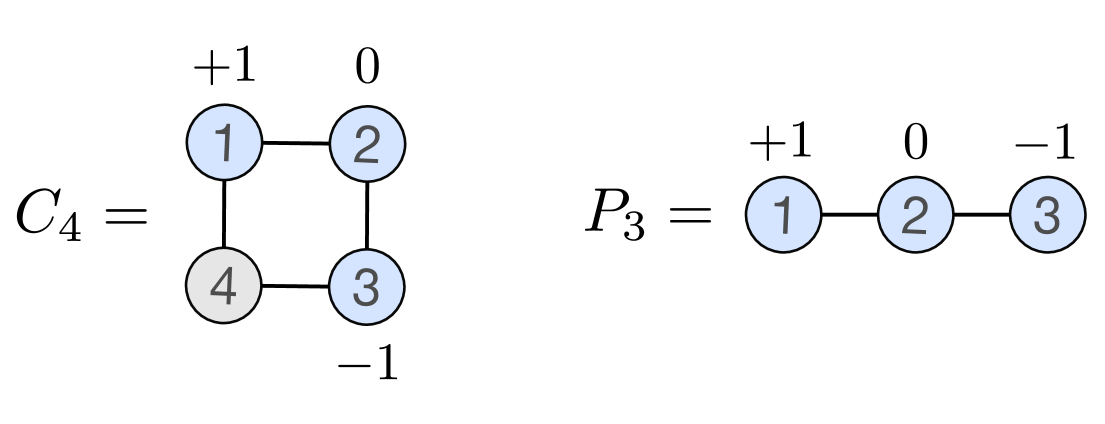
Figure 4: An example of an eigenpair-sharing subgraph is the path graph with 3 vertices, $P_{3}$, which is a subgraph of the cycle graph with 4 vertices, $C_{4}$. The graph $C_{4}$ has the adjacency spectrum $\{-2,0,0,2\}$, while $P_{3}$ has the spectrum $\{-\sqrt{2},0,\sqrt{2}\}$. They share the same eigenvalue $0$ and the (unnormalized) eigenvector $(+1,0,-1)^{T}$ upon appending zero on the 4th basis. The weights of the eigenvector are drawn as the numbers beside the corresponding vertices. Consequently, the weights on the 1st and 3rd vertices cancel out at the 4th vertex.

Although the graph is considered to be connected in our study, there can be induced subgraphs (or simply subgraphs) sharing the same eigenpairs with the entire graph $G$ with $N_{G}$ vertices. These special eigenvectors are localized on a subset of vertices $V^{\prime}\subseteq V$, inducing a subgraph $G^{\prime}=G[V^{\prime}]$ with $N_{G^{\prime}}$ vertices, which consists of the vertex set $V^{\prime}$ and all edges in $E$ with both endpoints in $V^{\prime}$. Remarkably, these eigenvectors can be comprehended through a $N_{G}\times N_{G}$ block matrix model,

$$\begin{pmatrix}A_{G^{\prime}}&K\\ K^{T}&A_{G-G^{\prime}}\end{pmatrix}\begin{pmatrix}\textbf{x}\\ 0\end{pmatrix}=\begin{pmatrix}A_{G^{\prime}}\textbf{x}\\ K^{T}\textbf{x}\end{pmatrix}=\begin{pmatrix}\mu\textbf{x}\\ 0\end{pmatrix}\text{,}$$ (4)

where $A_{G^{\prime}}$ and $A_{G-G^{\prime}}$ are square matrices with dimension $N_{G^{\prime}}$ and $N_{G-G^{\prime}}$ respectively. In general, $N_{G^{\prime}}\neq N_{G-G^{\prime}}$, making $K$ generally non-square. The last equality in Eq. (4) assumes that the submatrix $A_{G^{\prime}}$ coincidentally shares the same eigenvalue $\mu$ and eigenvector x (up on appending zeros) with the full matrix. Consequently, the eigenvector x must vanish at the outer boundary of the subgraph $G^{\prime}$ induced by $A_{G^{\prime}}$, i.e., $K^{T}\textbf{x}=0$. In other words, the eigenvector x is localized within the subgraph $G^{\prime}$. We refer to these interference-caged eigenvectors, which are shared by the subgraph and the parent graph, as the inteference-caged quantum many-body scars (ICQMBS), and the condition due to interference $K^{T}\textbf{x}=0$ as the interference-caged condition at the outer boundary.

It should be evident that the subgraphs having shared eigenpairs with connected parent graphs exhibit intrinsic distinctions from subgraphs having shared eigenpairs due to the disconnectedness of their parent graphs. When $K=0$, the parent graph is formed by disconnected components. This is the topological trivial case where the subgraphs share eigenvalues with the parent graph due to the disconnectedness. That usually happens when there is a symmetry of the system, or there are non-trivial topological sectors in the Hilbert space. The destructive interference occurring at the outer boundary of $G^{\prime}$ forms the foundation for the observed non-thermalizing behavior in QMBS, confining them within a relatively compact support on the Fock space graph. These delicate cancellations, however, serve as indicators of the underlying symmetries inherent in the graph. Nevertheless, the matrix model presented in Eq. (4) does not offer a method to identify any hidden subgraphs displaying these characteristics. Hence, further analysis of the graph’s symmetries analogous to crystalline symmetries in flat-band physics is warranted. One natural candidate to capture the concept of symmetry for a general complex graph is the graph automorphism that we will discuss in the next subsection.

III.3 Simplification of the interference-caged condition and the graph automorphism

Once the interference-caged condition is formulated, the remaining task is to devise a protocol to identify ICQMBS. One of the important tactics for exploring new physics is the principle of symmetries, which minimizes the required structure for certain phenomena. In the study of QMBS, the principle is challenged as the existence of QMBS is related to symmetries of the Hamiltonian in a subtle and convoluted fashion. In the case of ICQMBS, the local topological structure of the Fock space graph is relevant. Therefore, instead of analyzing the symmetries of a Hamiltonian, one should focus on the symmetries defined on a graph, the graph automorphism.

We will use undirected graphs with uniform weights on the edges to demonstrate the nature of the problem. We start the section with a brief introduction of the graph automorphism, which describes the equivalence principle between vertices that kept the adjacency matrix of the graph invariant. To make the later discussion clear, symmetries specifically referred to the physical operations that kept the Hamiltonian invariant, and graph symmetries, or graph automorphism, are used to describe the equivalence principle that kept the adjacency matrix of the graph invariant.

Once the terminology is clearly defined, we discuss the basic idea to simplify the search for the interference pattern on bipartite graphs using the coloring trick. Even though the protocol does not exploit the full power of graph automorphism, the algorithm is surprisingly efficient in identifying the ICQMBS for specific models in Sec. VI. Furthermore, the coloring trick demonstrates the nature of the problem and serves as a stepping stone to the refined description of the graph automorphism analysis.

With the intuition from the coloring trick, we formulate the task in terms of the graph automorphism. The general algorithm to identify the interference patterns based on graph automorphism is an intriguing combinatorial problem that we have not yet completely solved. Therefore, we provide some graph automorphism-based constraints that will be helpful for future algorithm development and leave the problem for future investigation.

III.3.1 Automorphism of a graph

The spectral properties of a graph reflect the underlying graph symmetries, manifesting in the high multiplicity of degenerate eigenvalues [116, 117]. The notion of graph symmetry is encapsulated by graph automorphism, which represents a permutation of vertices while maintaining adjacency; vertices can be arbitrarily relabeled, with adjacency remaining unchanged. For example, Fig. 5 demonstrates the possible permutations of vertex labeling for the cycle graph $C_{4}$. Although there are 24 possible permutations for relabeling the vertices, only 8 of them preserve the adjacency relations.

[] []

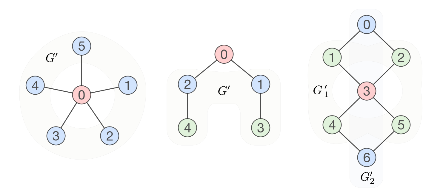
Figure 5: Illustration of graph automorphisms. (a) The cycle graph $C_{4}$ can be relabeled in $4!=24$ possible permutations, but only 8 permutations preserve adjacency (shown in the dashed box), forming the automorphisms of $C_{4}$. (b) Three example graphs are colored according to their orbits, where vertices of the same color are related by automorphisms and can be relabeled interchangeably.

All these permutations form an automorphism group of a graph $G$, denoted as $\text{Aut}(G)$. In matrix terms, this implies a permutation matrix $P$ that commutes with the adjacency matrix, $AP=PA$. Consequently, if $(\mu,\textbf{x})$ is an eigenpair of $A$, then $(\mu,P\textbf{x})$ will be another eigenpair, provided that x and $P\textbf{x}$ are linearly independent (not always the case). In particular, the orbit of a vertex $v$ is the set of vertices to which $v$ can be moved by an automorphism $\sigma\in\text{Aut}(G)$, that is,

$$\{\sigma(v)\text{ | }\sigma(v)\in\text{Aut}(G)\}\text{.}$$ (5)

The orbit represents structurally indistinguishable vertices under automorphism, contributing to redundant eigenvalues. We, therefore, treat orbits as the fundamental units in a graph. See Fig. 5 for the examples. The orbits will serve as the fundamental units for the general search of interference patterns on undirected graphs. However, before entering the general description of the problem, we will start the analysis from a simpler but inspiring protocol in the next section.

III.3.2 Searching of ICQMBS via pairwise cancellation and OBDHS

Before describing the search protocol, we introduce the coloring of a graph as a convenient tool for partitioning its vertices. This method is based on the expectation that the simplest subgraphs hosting ICQMBS are formed by destructive interference related to the structure of the Fock space graph. When a graph exhibits certain structural features, such as bipartiteness, its vertices can be subdivided into sets that can be numerically analyzed for cancelability at the outer boundary. The coloring trick can be understood as a convenient approach to using partial information of the graph automorphism. It will serve as a stepping stone to understand the proposed graph automorphism analysis later. While this method may not always identify the optimal subgraph, as there can be irrelevant and removable orbits that do not contribute to ICQMBS, it is generally effective in finding potential subgraphs that host ICQMBS, with the necessity of a subsequent test for the interference-caged condition.

Specifically, we assign individual colors to each vertex based on these structural features, effectively partitioning the vertex set $V$ into $m$ disjoint subsets, $V=V_{1}\cup\cdots\cup V_{i}\cup\cdots\cup V_{m}$ with $V_{i}\cap V_{j}=\emptyset$ when $i\neq j$. In later graph automorphism analysis, each set $V_{i}$ will be further subdivided into orbits. Once the coloring (or partitioning) is established, we can identify potential subgraphs whose eigenvectors may vanish at their outer boundaries. In practice, we examine the bipartite graph and the order-by-disorder mechanism in the Hilbert space (discussed in Sec. IV.4). These two graph properties can be leveraged to assign colors, yielding subgraphs for subsequent testing. Although this approach still requires diagonalizing the adjacency matrix of each corresponding subgraph and examining the cancelability of the eigenvectors at the outer boundary, the size of these subgraphs is typically much smaller, enabling the identification of QMBS at a lower computational cost. More concrete examples will be provided in the next section, Sec. III.3.3, for bipartite graphs, as well as in Sec. V and Sec. VI, where we explore specific lattice models.

III.3.3 Bipartite graphs

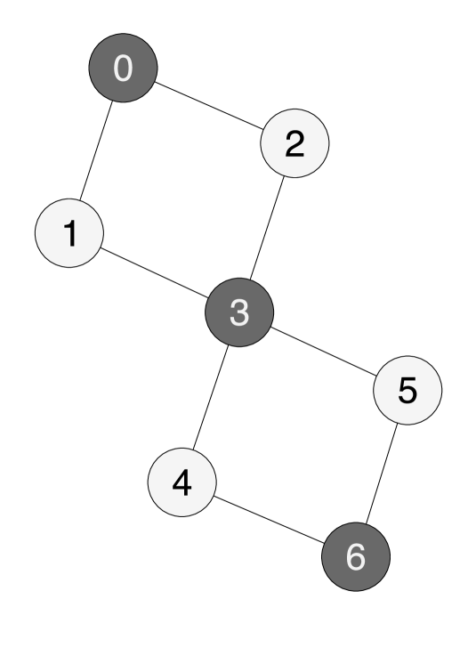
(a)

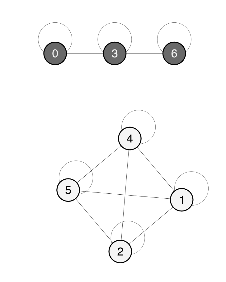
(b)

Figure 6: An illustration of (a) a bipartite graph $G$ colored in black and white according to its bipartite subsets, and (b) its bipartite projection $G^{2}$, which divides the vertices into two distinct, disconnected subgraphs. Note that a bipartite graph contains no self-loop. However, the bipartite projection always contains self-loops since every vertex must be connected with itself by a two-step move.

For certain limits of the lattice models that we have considered in Sec. V and Sec. VI, they exhibit the particle-hole symmetry generated by the parity (or chiral) operator $C$, which anti-commutes with the Hamiltonian, $\{H,C\}=0$. Consequently, this implies a symmetric spectrum about zero energy [118]. In graph theory, this manifests as bipartiteness, where vertices can be partitioned into two subsets. Equivalently, we can interpret this as a 2-coloring problem, where each subset of the bipartition is represented by a distinct color. To avoid confusion with other coloring schemes in later sections, we will reserve black and white specifically to denote the two subsets of a bipartite graph, $G=\{V_{b},V_{w},E\}$. The highly degenerate zero modes can be seen as the perfect destructive interference between these two subsets, while also supporting QMBS localized in the respective subset.

Once the two subsets are found, the adjacency matrix $A$ can be expressed on the basis sorted by its two subsets, leading to

$$\begin{pmatrix}O&K_{\text{b}}\\ K_{\text{b}}^{T}&O\end{pmatrix}\begin{pmatrix}\textbf{x}\\ \textbf{y}\end{pmatrix}=\begin{pmatrix}K_{\text{b}}\textbf{y}\\ K_{\text{b}}^{T}\textbf{x}\end{pmatrix}=\mu\begin{pmatrix}\textbf{x}\\ \textbf{y}\end{pmatrix}\text{,}$$ (6)

where the bi-adjacency matrix $K_{\text{b}}$ is generally a non-square matrix. It can be immediately seen that $(\textbf{x},-\textbf{y})^{T}$ forms another eigenvector with the eigenvalue $-\mu$. The $\pm\mu$-eigenvectors are related by the parity operator $C=\text{diag}(I,-I)$, such that $C(\textbf{x},\textbf{y})^{T}=(\textbf{x},-\textbf{y})^{T}$. In either case, unless the eigenvector of each respective subset, i.e. x and y, both vanishes on the opposite subset by $K_{\text{b}}$ and its transpose, $\mu$ must be non-zero regardless of its sign.

Consequently, the induced subgraph by $V_{b}$ or $V_{w}$ consists of only isolated vertices, and their cancelability at the outer boundary is fully determined by the null space of $K_{\text{b}}$ and $K_{\text{b}}^{T}$. Without the loss of generality, we typically choose the zero-eigenvectors to be either $(\textbf{x},0)^{T}$ or $(0,\textbf{y})^{T}$, subject to $K_{\text{b}}^{T}\textbf{x}=0$ and $K_{\text{b}}\textbf{y}=0$, respectively. While in an ED study, one often obtains the linear superposition of these two. This choice is beneficial because it does not require solving the null space of the entire adjacency matrix $A$, but only the null space of the bi-adjacency matrices $K_{\text{b}}$ and $K_{\text{b}}^{T}$, requiring a lower computational cost. Although as discussed in Sec. III.3.2, the induced subgraph by $V_{b}$ or $V_{w}$ may not be optimal, consisting of orbits that do not contribute to QMBS. To the best of our knowledge, this is the simplest approach without diving into the detailed structure of $\text{Aut}(G)$.

Generally, it is often preferred to compute the zero-eigenvectors of $K_{\text{b}}K_{\text{b}}^{T}$ (and $K_{\text{b}}^{T}K_{\text{b}}$), as the singular value decomposition of $K_{\text{b}}$ (and $K_{\text{b}}^{T}$) is directly related to the eigenvalue decomposition of these matrices. This approach is beneficial because $K_{\text{b}}K_{\text{b}}^{T}$ is a square matrix, and can be interpreted as a graph. The matrix $K_{\text{b}}K_{\text{b}}^{T}$ also has a natural description on the bipartite graph $G$. Consider a walker on the graph, initially located at vertex $v_{i}$ (and equivalently, the basis $\hat{e}_{i}$). The operation $A\hat{e}_{i}$ denotes a one-step move from $v_{i}$ to its adjacent vertices. Similarly, the square of the adjacency matrix, $A^{2}$, characterizes a two-step move. For a bipartite graph, this manifests as the walker returning to the starting subset (in either black or white). This is termed as the bipartite projection $G^{2}$. Consequently, $G^{2}$ naturally separates into two disconnected subgraphs, each corresponding to $V_{b}$ and $V_{w}$ of the bipartition, as illustrated in Fig. 6. Additionally, each vertex of $G^{2}$ has a self-loop weighted by its original degree in $G$, representing the number of possible paths for returning to the same vertex in two steps, which is given by $(A^{2})_{ii}$.

Finally, we note that the two bipartite subsets, $V_{b}$ and $V_{w}$, can also be identified through breadth-first search (BFS), a method commonly implemented in many graph analysis software tools.

III.3.4 Graph automorphism and the destructive interference boundary

Corollary III.0.1.

Vertices within the same automorphism orbit have the same degree.

The search for orbits provides an intuitive way to form the localizable (or interference-caged) eigenvector(s) on the subgraph. For the unweighted graphs, we summarize this principle as follows:

Lemma III.1.

Given a subgraph $G^{\prime}$, if for every vertex $v_{i}$ in the inner boundary of $G^{\prime}$, there exists at least one automorphism partner $\sigma(v_{i})\in G^{\prime}$, such that $v_{i}$ and $\sigma(v_{i})$ are uniformly connected to the same vertices $\{u_{i}\}$ on the outer boundary of $G^{\prime}$ (which stays unchanged under $\sigma$), then $G^{\prime}$ possesses localizable eigenvector(s).

Readers can verify this principle by examining Fig. 5. For example, for the star graph $S_{5}$ on the left of Fig. 5, it is possible to assign weights to the five blue vertices such that they cancel out at the red vertex. However, since the red vertex lacks an automorphism partner sharing the same neighbors, it cannot host localizable eigenvectors. Similarly, for the tree graph in the middle of Fig. 5, both the blue and green orbits are uniformly connected to the red vertex (with the green orbit effectively connecting to the red vertex with zero weights), allowing them to support localizable eigenvectors. This principle can also be extended to weighted graphs, although the possibility of cancellation at the outer boundary will depend on the weights and their respective signs.

While being less intuitive, there is another mechanism that can also host localizable eigenvectors. As depicted on the right of Fig. 5, the red and blue vertices are uniformly connected to the green vertices, allowing to form a localizable eigenvector, even though the red and blue vertices belong to different automorphism orbits. This is summarized as follows:

Lemma III.2.

Given a subgraph $G^{\prime}$, if every orbit in the inner boundary of $G^{\prime}$ is connected to a common orbit $\{\sigma(u)\}$, which forms the outer boundary of $G^{\prime}$, then $G^{\prime}$ possesses localizable eigenvector(s).

Nevertheless, finding a subgraph satisfying these features requires a detailed analysis of the group elements of $\text{Aut}(G)$ and their support. While this analysis can be performed using computational group theory, it remains a highly non-trivial combinatorial problem. Therefore, in Sec. III.3.3, Sec. V and Sec. VI, we will primarily focus on bipartite graphs $G=\{U,V,E\}$, where vertices are partitioned into two subsets, $U$ and $V$. Edges exclusively connect vertices between these subsets, with no edges connecting vertices within the same subset. The bipartite graphs are considered simpler because the localizable subgraph can only appear in either subset $U$ or $V$. Although we will also consider a few non-bipartite graphs that contain localizable subgraphs, a general search protocol remains unclear.

It is also worth noting the relationship between conventional lattice symmetries and graph automorphisms. All conventional global lattice symmetries, which are specific types of basis permutations, can be identified as a subgroup of $\text{Aut}(G)$ and can still be defined in the thermodynamic limit.

IV Formal perspectives of interference-caged quantum many-body scars

Before entering the model-specific sections, we first formalize ICQMBS to connect physical intuition and specific models with a unified framework. Our earlier discussion focused primarily on systems with time-reversal and crystalline symmetries, where the Fock space graphs have equal, real-valued edge weights. This simplification manifests how the local topology of the Fock space graph enters the analysis of non-thermal states. However, such simplifications are not fundamentally required. We will discuss how to relax these symmetry requirements and generalize ICQMBS to include topologically non-trivial cases. To place our findings in context, we compare the intrinsic features of ICQMBS with other existing general descriptions of QMBS, such as the projector embedding procedure [82] and approaches based on higher symmetry algebra [68, 69, 70, 71, 72, 73, 74]. We further highlight how ICQMBS differs from existing Hilbert space fragmentation phenomena, emphasizing its role as an inherently emergent quantum phenomenon. The many-body interference blocks the coupling between states instead of relying on constraints to decouple the many-body states.

The formal framework of ICQMBS relies on analyzing the interference zeros of an eigenstate within the Fock space graphs. By examining the structure of these interference zeros, we distinguish and classify ICQMBS into two main types: regional ICQMBS and extended ICQMBS. The regional ICQMBS are further divided into topological ICQMBS (tICQMBS) and simple ICQMBS (sICQMBS) based on their robustness due to local topology. For tICQMBS, the interference zeros must effectively cage the weights of the wave function on a support that is vanishingly small compared with the entire graph. This formalism, rooted in the concept of interference zeros, provides new insights into the stability of tICQMBS through local topological properties. In contrast, sICQMBS are generally fragile to real space perturbations.

We begin the section with an introduction to interference zeros in Sec. IV.1. After briefly reviewing the projector embedding approach [82], we formulate the relation between interference zeros and ICQMBS. In this discussion, we emphasize our formally similar yet fundamentally different proof of the non-thermal behavior of ICQMBS, along with a more refined classification of ICQMBS based on the structure of interference zeros. In Sec. IV.2, we discuss why ICQMBS is beyond the approaches based on higher symmetry algebra [68, 69, 70, 71, 72, 73, 74] and the stability due to local topology. In Sec. IV.3, we discuss ICQMBS and the Hilbert space fragmentation. In particular, we want to emphasize that tICQMBS represents an emergent quantum phenomenon arising from constraints with no classical counterpart. Finally, in Sec. IV.4, we discuss the order-by-disorder phenomena in Hilbert space (OBDHS) and how it can be understood within the ICQMBS framework. Therefore, the natural connection with local topology makes the ICQMBS mechanism unique in the study of weak ergodicity-breaking systems.

IV.1 Interference-caged quantum many-body scars and the interference zeros

The projector embedding approach, introduced by Shiraishi and Mori [82], relies on the local projectors, $\widehat{P}_{j}$, to decouple the embedded states with other thermal states. The non-thermal eigenstate violates ETH since the vanishing expectation value of the local projector, $\widehat{P}_{j}$. In this section, we briefly review the essence of the projector embedding approach and introduce proof of the non-thermal nature of ICQMBS based on the interference zeros. Parallel with the projector embedding approach, ICQMBS is non-thermal since the vanishing expectation value of the local operator, $\widehat{Z_{h}}$, captures the interference zero on state $|h\rangle$. The physics of the two proofs is fundamentally different, albeit formally similar.

IV.1.1 Review of the projector embedding approach

Considering a closed quantum many-body system described by a Hamiltonian, $\widehat{H}_{SM}$, and a many-body Hilbert space, $\mathcal{H}_{SM}$, one can use the following procedure to design the Hamiltonian and embed the frustration-free non-thermal states into the spectrum. For an arbitrary set of local projectors, $\widehat{P}_{j}$ where $j=1\sim O(N_{\Omega})$, that does not commute with each other in general, one can use the projectors to construct a sub-Hilbert space $\mathcal{T}\subset\mathcal{H}_{SM}$ where all the states in this sub-Hilbert space can be eliminated by any projectors in this set. i.e., $|\Psi_{\mathcal{T}}\rangle\in\mathcal{T}$ if $\widehat{P}_{j}|\Psi_{\mathcal{T}}\rangle=0$ for any $j$. If the sub-Hilbert space $\mathcal{T}$ is non-empty, one can construct a Hamiltonian that hosts the eigenstates $|\Psi_{\mathcal{T}}\rangle\in\mathcal{T}$ as

$$\widehat{H}_{SM}=\sum_{j}\widehat{P}_{j}\widehat{h}_{j}\widehat{P}_{j}+\widehat{H}^{\prime}\text{ with }\left[\widehat{H}^{\prime},\widehat{P}_{j}\right]=0\text{.}$$ (7)

Here, $\widehat{h}_{j}$ is an arbitrary local Hamiltonian that, in general, has eigenstates satisfying ETH. Furthermore, $\left[\widehat{H}^{\prime},\widehat{P}_{j}\right]=0$ guarantee that $\mathcal{T}$ is invariant under the mapping of $\widehat{H}_{SM}$. The projector embedding approach is closely related to the frustration-free Hamiltonians when $\widehat{H}^{\prime}=0$ [82, 83] since $\widehat{H}_{j}\equiv\widehat{P}_{j}\widehat{h}_{j}\widehat{P}_{j}$ eliminates all states in $\mathcal{T}\;\forall j$ as in the frustration-free models.

By construction, one can show that $|\Psi_{\mathcal{T}}\rangle$ is a non-thermal state since the vanishing expectation value for the local operators $\widehat{P}_{j}$ violates the ETH. The number of projectors does not enter the argument of non-thermal behavior. Even if there is only one $\widehat{P}_{j}$ that eliminates the embedded state, it is enough to prove the embedded state is not thermal. The number of projectors $\widehat{P}_{j}$ delicately enters the argument through the construction of the form of the Hamiltonian, which, from the perspective of hosting QMBS, is not a required condition. The decoupling between the thermal state and the embedded non-thermal state is established by the projector operator $\widehat{P}_{j}$ without explicitly discussing the physical origin of $\widehat{P}_{j}$ and makes it a versatile description for QMBS.

The projector embedding approach serves as a description of the emergent non-thermal subspace through the lens of frustration-free Hamiltonian, but its connection to the physical origin of the non-thermal state is not immediately clear. Furthermore, generally identifying the corresponding frustration-free Hamiltonian is actually highly non-trivial since determining whether a Hamiltonian is frustration-free is a quantum satisfiability (QSAT) problem that is known to be QMA₁ complete [119, 120, 121, 122]. It is widely believed to be intractable and attracts attention in the study of quantum matter, quantum computation, and complexity theory [123, 124, 125]. From this perspective, the construction is limited by our understanding of frustration-free Hamiltonians, and there are certainly QMBS that are not frustration-free.

IV.1.2 Interference zeros and violation of ETH

The argument of ICQMBS in Sec.III is inspired by the observation of the low entanglement entropy property of QMBS. The small support for the eigenstate from the product state basis naturally leads to the expected low entanglement entropy. However, how this intuitive picture connects with the non-thermal behavior is not rigorously established in previous sections. Furthermore, it is not clear how to remove the effects of symmetries and derive a more general mechanism. Therefore, we would like to develop a formal description for ICQMBS in this section to explicitly argue the non-thermal nature and core structure that is independent of the symmetries. A key structure for our argument is the interference zeros or the eigenstate zeros. In the following discussion, we consider the symmetry sectors that are labeled by quantum numbers such that the basis in the sectors can still be represented by product states.

The interference zeros of a mid-spectrum eigenvector can be understood using the Fock space graph. Without losing generality, we consider the Fock space interference to happen in a connected component of the Fock space graph on the product state basis. When representing an eigenstate on the Fock space graph, every vertex has the corresponding weights of the eigenstate. If one of the vertices has zero weight, it means after we apply the Hamiltonian to this eigenstate, the fictitious particles will tunnel from the neighboring vertices with the corresponding weights and eliminate the weights on the target vertex due to perfect destructive interference. Therefore, the vertices with zero weight are considered as the interference zeros, or the eigenstate zeros, of the eigenstates. Formally one can define an operator $\widehat{I_{h}}$ to detect an interference zero on basis vector $|h\rangle$ as

$$\widehat{I_{h}}\equiv\sum_{v_{j}\in_{\widehat{H}}\partial h}|v_{j}\rangle A_{v_{j},h}\langle h|+|h\rangle A_{h,v_{j}}\langle v_{j}|\text{.}$$ (8)

Here, ${}_{\widehat{H}}\partial h$ means the set of neighboring vertices (one-step connected vertices) of $|h\rangle$ on the Fock space graph of Hamiltonian $\widehat{H}$. $A_{v_{j},h}=\langle v_{j}|\widehat{H}_{\Omega}|h\rangle=A_{h,v_{j}}^{*}$ for Hermitian Hamiltonians. For an eigenstate $|E^{(\zeta)}\neq 0\rangle=\sum_{u_{j}}c^{(\zeta)}_{u_{j}}|u_{j}\rangle$ at finite energy density with interference zero at $|h\rangle$, $c^{(\zeta)}_{h}=\langle h|E^{(\zeta)}\rangle=0$. That is,

$$\langle h|\widehat{H}|E^{(\zeta)}\rangle =E^{(\zeta)}\langle h|E^{(\zeta)}\rangle=E^{(\zeta)}c^{(\zeta)}_{h}$$ (9)

$$=\sum_{u_{j}}A_{h,u_{j}}c^{(\zeta)}_{u_{j}}=\sum_{u_{j}\in_{\widehat{H}}\partial h}A_{h,u_{j}}c^{(\zeta)}_{u_{j}}=0\text{.}$$

In the second line, we replace the $\sum_{u_{j}}$ with $\sum_{u_{j}\in_{\widehat{H}}\partial h}$ using the Fock space graph interpretation, vertices connected with $|h\rangle$ through the non-zero matrix element of the Hamiltonian must be at the boundary of $|h\rangle$. Using this condition, we can simplify $\widehat{I_{h}}|E^{(\zeta)}\rangle$ as

$$\widehat{I_{h}}|E^{(\zeta)}\rangle =\left(\sum_{v_{j}\in_{\widehat{H}}\partial h}|v_{j}\rangle A_{v_{j},h}\langle h|+h.c.\right)\left(\sum_{u_{j}}c^{(\zeta)}_{u_{j}}|u_{j}\rangle\right)$$ (10)

$$=\sum_{v_{j}\in_{\widehat{H}}\partial h}A_{h,v_{j}}c^{(\zeta)}_{v_{j}}|h\rangle=0$$

The operator $\widehat{I_{h}}$ identifies the interference zero on $|h\rangle$ explicitly. If an eigenstate $|E^{(\zeta)}\rangle$ has an interference zero on basis vector $|h\rangle$, it means $\widehat{I_{h}}|E^{(\zeta)}\rangle=0$. When $\sum_{v_{j}\in_{\widehat{H}}\partial h}A_{h,v_{j}}c^{(\zeta)}_{v_{j}}=0$ for non-zero $c^{(\zeta)}_{v_{j}}$, we consider the interference zero to be non-trivial. If $\sum_{v_{j}\in_{\widehat{H}}\partial h}A_{h,v_{j}}c^{(\zeta)}_{v_{j}}=0$ holds when $c^{(\zeta)}_{v_{j}}=0$, we consider the interference zero to be trivial. The notion can be extended to general cases with multiple interference zeros. Therefore, we focus on the physics with single interference zero without losing generality in the following discussion.

Since vertices $\{|v_{j}\rangle\}$ are connected to $|h\rangle$ through the local Hamiltonian, $\widehat{H}$, we expect $\{|v_{j}\rangle\}$ and $|h\rangle$ only differ locally. The common portion of the product states $\{|v_{j}\rangle\}$ and $|h\rangle$ is represented by $|\{\bigcap_{j}v_{j}\}\cap h\rangle\equiv|\beta_{\widehat{H}}(h)\rangle$ where we explicitly show the dependence of $\widehat{H}$ and $|h\rangle$ for the common portion of the product states. Here, we define the sub-Hilbert space $\mathcal{H}_{\Lambda}$ supported by sub-system $\Lambda$ as the minimum support of the product state $|\beta_{\widehat{H}}(h)\rangle$. i.e. $|\beta_{\widehat{H}}(h)\rangle\in\mathcal{H}_{\Lambda}\equiv\bigotimes_{\mathbf{r}\in\Lambda}\mathcal{H}_{\mathbf{r}}$ where $\Lambda\subset\Omega$ and $\Lambda$ is chosen to be as small as possible. The operator $\widehat{I_{h}}$ can be expressed as

$$\widehat{I_{h}}=\left(\widehat{P}_{\beta_{\widehat{H}}(h)}\right)_{\Lambda}\otimes\left(\widehat{Z_{h}}\right)_{\Omega-\Lambda}\text{.}$$ (13)

Here, we can notice $\widehat{I_{h}}$ is a direct product of two operators acting on $\mathcal{H}_{\Lambda}$ and $\mathcal{H}_{\Omega-\Lambda}$. The first part is the non-local projector, $\widehat{P}_{\beta_{\widehat{H}}(h)}$, that projects to the common product state $|\beta_{\widehat{H}}(h)\rangle$ in $\mathcal{H}_{\Lambda}$. The other part is the local operator, $\widehat{Z_{h}}$, that acts non-trivially on the supplement of $\mathcal{H}_{\Lambda}$ , $\mathcal{H}_{\Omega-\Lambda}$.

In general, $\widehat{I_{h}}$ is a non-local operator due to the non-local projector acting on $\mathcal{H}_{\Lambda}$. To demonstrate the connection of interference zeros and the non-thermal nature of ICQMBS, we devise a local operator, the reduced interference zero operator $\widehat{Z^{(R)}_{h}}$, that partially captures the structure of destructive interference near state $|h\rangle$.

$$\widehat{Z^{(R)}_{h}} \equiv\left(\mathbf{1}\right)_{{\Lambda}}\otimes\left(\widehat{Z_{h}}\right)_{\Omega-\Lambda}=\widehat{I_{h}}+\widehat{\overline{I_{h}}}$$ (14)

with

$$\widehat{\overline{I_{h}}} =\left(\widehat{Q}_{\beta_{\widehat{H}}(h)}\right)_{\Lambda}\otimes\left(\widehat{Z_{h}}\right)_{\Omega-\Lambda}$$

$$\left(\mathbf{1}\right)_{{\Lambda}} =\left(\widehat{P}_{\beta_{\widehat{H}}(h)}+\widehat{Q}_{\beta_{\widehat{H}}(h)}\right)_{\Lambda}\text{.}$$

To determine whether a finite energy-density eigenstate with multiple nontrivial interference zeros on vertices $|h_{j}\rangle$, denoted as $|E^{(\zeta)}(\left\{h_{j}\right\})\rangle$, is thermal or not, we can calculate the expectation value of the reduced interference zero operators. Without losing generality, let’s consider the expectation value of the reduced interference zero operator for a non-trivial interference zero at vertex $|h_{a}\rangle\in\{|h_{j}\rangle\}$, i.e., $\langle E^{(\zeta)}(\left\{h_{j}\right\})|\widehat{Z^{(R)}_{h_{a}}}|E^{(\zeta)}(\left\{h_{j}\right\})\rangle=\langle E^{(\zeta)}(\left\{h_{j}\right\})|\widehat{I_{h_{a}}}+\widehat{\overline{I_{h_{a}}}}|E^{(\zeta)}(\left\{h_{j}\right\})\rangle$.

The first term, $\widehat{I_{h_{a}}}|E^{(\zeta)}(\left\{h_{j}\right\})\rangle=0$, vanishes by construction. We will discuss the conditions that $\widehat{\overline{I_{h_{a}}}}|E^{(\zeta)}(\left\{h_{j}\right\})\rangle=0$. In short, the two parts of $\widehat{\overline{I_{h_{a}}}}$ could act like projectors to the ICQMBS in subsystem $\Lambda$ and $\Omega-\Lambda$ respectively.

The first case is the regional ICQMBS. If the weights of the state $|E^{(\zeta)}(\left\{h_{j}\right\})\rangle$ are restricted in a portion of the graph near $|h_{a}\rangle$ where $\left(\widehat{Q}_{\beta_{\widehat{H}}(h_{a})}\right)_{\Lambda}\otimes\left(\widehat{I}_{h_{a}}\right)_{\Omega-\Lambda}|E^{(\zeta)}(\left\{h_{j}\right\})\rangle=0$ simply because there are no weights to be transferred by $\widehat{I_{h}}$ once it is projected by $\left(\widehat{Q}_{\beta_{\widehat{H}}(h_{a})}\right)_{\Lambda}$ in the connected component, i.e., if the eigenstate $|E^{(\zeta)}(\left\{h_{j}\right\})\rangle$ has non-trivial interference zeros on $|h_{j}\rangle$ and overwhelmingly trivial interference zeros on other connected vertices outside the relevant vertices for non-trivial interference zeros, $\langle E^{(\zeta)}(\left\{h_{j}\right\})|\widehat{Z^{(R)}_{h_{a}}}|E^{(\zeta)}(\left\{h_{j}\right\})\rangle=0$. Then, the finite energy density eigenstate $|E^{(\zeta)}(\left\{h_{j}\right\})\rangle$ must be a non-thermal state due to its vanishing expectation value of the local operator $\widehat{Z^{(R)}_{h_{a}}}$ violates the ETH. In this case, $\Omega\gtrapprox\Lambda$, $\Omega-\Lambda$ is small comparing with $\Lambda$ and $\Omega$.

The second case is the extended ICQMBS. If the operator $\left(\widehat{Z}_{h_{a}}\right)_{\Omega-\Lambda}$ acts like a local projector that eliminates the weights on other vertices outside the relevant vertices for non-trivial interference zero $|h_{a}\rangle$, $\langle E^{(\zeta)}(\left\{h_{j}\right\})|\widehat{Z_{h_{a}}}|E^{(\zeta)}(\left\{h_{j}\right\})\rangle=0$. In this case, we have $\langle E^{(\zeta)}(\left\{h_{j}\right\})|\widehat{Z^{(R)}_{h_{a}}}|E^{(\zeta)}(\left\{h_{j}\right\})\rangle=0$ again, and the same argument suggests the eigenstate violate ETH. Since the projector nature of the local operator $\widehat{Z_{h_{a}}}$ in this case, the vertices that do not participate in the destructive interference at $|h_{a}\rangle$ could have non-zero weights in general. Due to the fact that those vertices with non-zero weights could still couple with other vertices through the local operators in the Hamiltonian, the simplest way to make the eigenstate non-thermal is these local operators are actually responsible for other interference zeros. Therefore, all non-zero weight vertices are caged in an extensive region in the Hilbert space. That is, if the local operators that form the Hamiltonian acting on a finite energy-density eigenstate have only two effects: forming interference zeros, $\langle E^{(\zeta)}(\left\{h_{j}\right\})|\widehat{I_{h_{a}}}|E^{(\zeta)}(\left\{h_{j}\right\})\rangle=0$ , or eliminating the weight on vertices outside the local interference pattern, $\langle E^{(\zeta)}(\left\{h_{j}\right\})|\left(\widehat{Q}_{\beta_{\widehat{H}}(h_{a})}\right)_{\Lambda}\otimes\left(\widehat{I}_{h_{a}}\right)_{\Omega-\Lambda}|E^{(\zeta)}(\left\{h_{j}\right\})\rangle=0$. Therefore, unlike the regional ICQMBS, the extended ICQMBS have support on a finite fraction of the Fock space graph in the thermodynamic limit.

Here, we want to emphasize that the formal construction closest to our approach is the projector embedding approach, where the local projector has a vanishing expectation value. Similar to the projector embedding approach, symmetry does not enter the argument. However, our approach is fundamentally different from the projector embedding approach. First, the projector embedding construction is closely related to the frustration-free Hamiltonians. In our case, there is no explicit connection with the frustration-free Hamiltonians. In fact, [118] shows that one can use the destructive interference mechanism to understand the bond-bimagnon scar states in the $S=1$ XY spin chain which does not satisfy the frustration-free condition. The bond-bimagnon scar states are thus an example of the extended ICQMBS. Second, the local operator, $\widehat{Z^{(R)}_{h}}$, is in general not a projector. $\widehat{Z^{(R)}_{h}}$ manifests the physical meaning of how destructive interference decouples the non-thermal eigenstates from the thermal ones. Third, the analysis of regional ICQMBS also reveals the possibility of having robust QMBS due to the local topology of the Fock space graph, a non-trivial statement beyond the projector embedding approach. That is, if we deform the Hamiltonian while keeping the local interference pattern near the interference zeros invariant, the regional ICQMBS will remain non-thermal. Such deformation only needs to respect the local topology and can remove all kinds of symmetry structures or prerequisite algebraic structures. We will discuss the stability due to local topology in more detail later in Sec.IV.2. Fourth, the interference zero approach does not rely on the decomposition of Hamiltonians into specific algebraic forms related to higher symmetries or frustration-free expressions. In that sense, the criteria are not by design and can be applied to generic systems.

The general mechanism can applied to systems with different symmetries, dimensionalities, and dynamical constraints. The corresponding scar states could also have arbitrary energy densities. That suggests the mechanism might be useful to the understanding of isolated quantum many-body scars. However, due to the generality of this mechanism, it is difficult to devise a systematic protocol to identify those ICQMBS for generic systems. Nonetheless, we demonstrate that even without a practical protocol for locating interference zeros in general, standard linear algebra algorithms can be utilized for this purpose under specific conditions. Specifically, this involves analyzing the null space of $\widehat{O}_{\text{kin}}$, a task that standard linear algebra toolkits can efficiently handle. The detail of the process is discussed in Appendix B. More studies are warranted to find ICQMBS systematically. We will discuss specific models in one and two-dimensional systems in Sec. V and Sec. VI, where practical challenges will be discussed in detail.

IV.2 Symmetries and the topological stability of ICQMBS

Now we turn to the argument that the mechanism behind ICQMBS is distinct from the QMBS described by the algebra of higher symmetries such as the spectrum-generating algebra (SGA) [68, 69], group-invariant sectors [70, 71, 72], and quasisymmetry groups [73, 74]. The key ingredient in those approaches is established on the transformation property of the scar states dictates the decoupling between the thermal and the scar states via the algebra structure of the Hamiltonian. ICQMBS decoupled with the thermal eigenstates through a different mechanism. ICQMBS are superposition of the participating vertices $\{|u_{j}\rangle\}$, surrounded by the non-trivial interference zeros $\{|h_{j}\rangle\}$ where the interference is achieved by the weighted edges between $\{|u_{j}\rangle\}$ and $\{|h_{j}\rangle\}$. The only relevant information is the abstract local Fock space graph structure formed by the vertices and edges such that the local interference pattern is supported without specifying the physical correspondence of the vertices and the edges. That is, how the product state transforms under symmetry is irrelevant for ICQMBS. As long as the matrix elements provide the required local topology of the Fock space graph, ICQMBS will be realized.

For example, the relevant vertices could represent spin 1 spins, hard-core bosons, a many-body state with different magnitudes of spins, or states in a many-body Hilbert space without the direct product structure due to non-trivial constraints which transform very differently under the corresponding algebra of the symmetry. The edges connecting those vertices are just local terms with the corresponding physical interpretations. One does not need to require the Hamiltonian to satisfy a specific algebraic structure for the higher symmetries or a global symmetry to realize ICQMBS. As long as the abstract Fock space graph has the required local topology, ICQMBS will be realized. However, this possibility is overlooked, most likely due to the fact that it is challenging to achieve the required local topology for a many-body Hamiltonian. Also, adding terms that break the symmetry structure (either the true symmetry of the Hamiltonian or the higher symmetry with a specific algebraic structure) while keeping the local topology of the Fock space graph might not be feasible in most cases. Here, we just provide a trivial argument that there is no logical connection between the local Fock space topology and the algebraic structure of the Hamiltonian and the state since the graph structure does not rely on this information directly. To rationalize the statement, we will revisit this issue in the later sections using concrete examples in Sec. VI.

The study of the stability of QMBS has been explored extensively through the scope of forward scattering approximation [19], using Lieb-Robinson bounds [126], fidelity susceptibility analysis of the MPS [127] and non-Hermitian skin effects [128]. The stability of QMBS is not only important for fundamental reasons but also crucial for possible applications [32, 31]. Since the QMBS have different origins, the stability analysis, therefore, is strongly tied to the nature of the corresponding QMBS. We just argued that the existence of ICQMBS is not due to specific symmetry structures and is intrinsically different from the projector embedding cases. Therefore, the stability of ICQMBS also has distinct features compared with QMBS described in these cases. Specifically, we would like to emphasize the stability of ICQMBS from the perspective of local topology.

In Sec.IV.1.2, we discuss the interference zeros and how to use interference zeros to distinguish the regional ICQMBS and extended ICQMBS. The regional ICQMBS has a direct analogy with the strictly localized states in flat band physics where the support of the wave function occupied a vanishing portion of the Fock space graph at the thermodynamic limit [88]. Due to the tiny support, one has a large degree of freedom to deform the Fock space graph while keeping the local interference pattern of the regional ICQMBS intact, as we have learned in Ref. [88]. The strictly localized state is robust due to its local topology. It is tempting to ask a similar question here: is it possible that some regional ICQMBS is robust against real-space local perturbation since the local perturbation only alters the Fock space graph away from the interference region? We found the answer to be positive. This family of ICQMBS will have anomalously robust properties that are protected by the local topology. We dubbed such ICQMBS as topological ICQMBS(tICQMBS). Other regional ICQMBS without such topological protection will be dubbed as simple ICQMBS(sICQMBS). For the case of extended ICQMBS, it is not clear whether it is possible to add the real-space local perturbation without affecting the local interference pattern. We will leave this part for future studies.

The tICQMBS manifests the statement that algebra of higher symmetry and global symmetry are irrelevant for the ICQMBS. tICQMBS is robust against arbitrary real space local terms that only alter the Fock space graph with trivial interference zeros. Therefore, from the destructive interference picture, the real space local terms that break the algebra of higher symmetries and the global symmetry will not alter the original ICQMBS. Therefore, the Hamiltonian can break translation symmetry, time-reversal symmetry, and even unitarity but still host the same tICQMBS. To the best of our knowledge, QMBS with the disorder can be realized through the projector embedding approach [82] or the Onsager symmetry construction [93]. Here, we provide another mechanism to realize QMBS when translational symmetry is absent.

One can also ask a reversed question: given a caged wave function $|\phi_{caged}\rangle$, can one devise a Hamiltonian that host $|\phi_{caged}\rangle$ as a tICQMBS? From the interference zero structure discussed above, can we argue such construction exists and will be protected by the local topology of the Hamiltonian? Here, we give a heuristic argument that it is indeed possible.

For a caged state $|\phi_{caged}\rangle$ to be considered as tICQMBS, the relevant interference pattern must be local. Therefore, we expect to construct a Hamiltonian $\widehat{H}_{0}$ where the matrix elements are assigned by the interference pattern of $|\phi_{caged}\rangle$. The local Hamiltonian will not only assign the coupling for the relevant state of the $|\phi_{caged}\rangle$ but also assign couplings for the states that are away from the interference pattern in general. To make our discussion specific, the caged state is supported by the caged Hilbert space, $\mathcal{H}_{caged}$, formed by the basis with non-zero weight and non-trivial interference zeros connected with those basis. The Hamiltonian formed by local operators, $\widehat{\mathsf{h}}_{j}$, are supported by Hilbert space in a subsystem $B\subset\Omega$, $\mathcal{H}_{B}\equiv\bigotimes_{\mathbf{r}_{j}\in B}\mathcal{H}_{\mathbf{r}_{j}}$. That is,

$$\widehat{H}_{0} =\sum_{v_{j},v_{k}\in\mathcal{H}_{caged}}\mathsf{A}^{(0)}_{jk}|v_{j}\rangle\langle v_{k}|$$ (15)

$$+\sum_{v_{j},v_{k}\not\in\mathcal{H}_{caged}}A^{(0)}_{jk}|v_{j}\rangle\langle v_{k}|+\sum_{v_{j}\in\mathcal{H}_{caged},\atop v_{k}\not\in\mathcal{H}_{caged}}A^{(0)}_{jk}|v_{j}\rangle\langle v_{k}|$$

$$=\sum_{j=1}^{M}\widehat{\mathsf{h}}_{j}$$

Here, the design of $\mathsf{h}_{j}$ is not unique. It only requires the local interference pattern given by $|\phi_{caged}\rangle$ is recovered through part of the adjacency matrix, $\mathsf{A}^{(0)}$, that is within $\mathcal{H}_{caged}$. We assume $M\ll N_{\Omega}$ in order for $|\phi_{caged}\rangle$ to be considered as tICQMBS. The state $|\phi_{caged}\rangle$ will be an eigenstate of $\widehat{H}_{0}$ by design. $\widehat{H}_{0}$ fix part of the edges of the Fock space graph respecting the caged interference pattern. Now, one can include more edges by adding local operators $\widehat{\mathsf{h}}^{int}_{j}$ and $\widehat{\mathsf{h}}_{j}^{out}$ into the Hamiltonian $\widehat{H}_{0}$. Here, we require $\widehat{\mathsf{h}}^{int}_{j}$ to contribute edges connecting the trivial interference zeros outside of $\mathcal{H}_{B}$ and the non-trivial interference zeros within $\mathcal{H}_{B}$. $\widehat{\mathsf{h}}^{out}_{j}$ can only contribute edges connecting trivial interference zeros outside $\mathcal{H}_{B}$. We can construct a Hamiltonian, $\widehat{H}_{tICQMBS}$ , with arbitrary coefficients $\mu_{j},\nu_{j}$ as

$$\widehat{H}_{tICQMBS}=\widehat{H}_{0}+\sum_{j}\mu_{j}\widehat{\mathsf{h}}_{j}^{int}+\sum_{j}\nu_{j}\widehat{\mathsf{h}}_{j}^{out}\text{.}$$ (16)

The terms controlled by $\mu_{j}$ will only transfer weights between trivial and non-trivial interference zeros of $|\phi_{caged}\rangle$. The terms controlled by $\nu_{j}$ will only transfer weights between trivial interference zeros of $|\phi_{caged}\rangle$. Therefore, the Hamiltonian will host $|\phi_{caged}\rangle$ as an eigenvector by design. The real space perturbation respecting the interference pattern of $|\phi_{caged}\rangle$ will only alter the coefficients of $\mu_{j}$ and $\nu_{j}$ which will not change the structure of $|\phi_{caged}\rangle$. Therefore, $\widehat{H}_{tICQMBS}$ host $|\phi_{caged}\rangle$ as a tICQMBS that is robust against local topology preserving perturbations with finite energy density in general. There is no restriction on the algebraic structure of the Hamiltonian or further symmetry structure of the local operators $\widehat{\mathsf{h}}_{j}^{int}$ and $\widehat{\mathsf{h}}_{j}^{out}$. We expect one can embed $|\phi_{caged}\rangle$ in a background of finite energy density thermal states by a generic choice of $\mu_{j}$ and $\nu_{j}$.

In summary, time-reversal symmetry and crystalline symmetries are not essential to realize ICQMBS, even though some of the examples have those symmetries. tICQMBS is robust with all deformation of the Hamiltonian as long as the local interference pattern is preserved. Because of that, we can deform the Hamiltonian and break almost all the symmetries, including time-reversal symmetry and crystalline symmetries, by adding symmetry-breaking terms that preserve the local interference pattern. For example, the perturbation can be disorder terms that break the crystalline symmetries, Zeeman terms that break the time-reversal symmetry, or even dissipation .

IV.3 Hilbert space fragmentation, ICQMBS and thermodynamic limit

In the study of quantum ergodicity breaking for constrained systems, one encounters Hilbert space fragmentation [24, 25, 129], i.e. the situation that the Hilbert space splits into exponentially many dynamically disconnected parts. Therefore, the dynamics of different initial states could be drastically different depending on how the initial states are projected into the different dynamical sectors. When the fraction of ETH-violating eigenstates in such systems vanishes at the thermodynamic limit, we refer to the phenomena as weak Hilbert space fragmentation. Sometimes, weakly fragmented systems are considered examples of quantum many-body scars.

Here, we would like to consider if ETH is violated explicitly or spontaneously in a similar fashion as we discuss how symmetry is broken for a many-body state. If ETH is violated by identifiable immutable local configurations according to the dynamical constraints of the Hamiltonian beyond symmetry reasons, we said the ETH is explicitly violated by the evolution operator. For example, ETH is explicitly violated for the jammed states in [130]. On the other hand, if ETH violation cannot be understood in this way, the ETH is violated in a spontaneous fashion. To be more specific, the immutable local configurations due to constraints act like a classical hard divider that cuts the system into decoupled dynamical sectors in real space. For those systems, ETH is expected to be violated explicitly. From that perspective, ICQMBS is a state where ETH is spontaneously violated.

ICQMBS happens within dynamically connected sectors. The intriguing phenomenon is quantum mechanical and spontaneous due to the many-body destructive interference dynamically forbidden inclusion of certain basis vectors into ICQMBS. The closest analogy in the study of classical systems is the arch in jamming configurations. In the classical system, the arch in a jammed configuration is a local structure that is spontaneously generated and forbids dynamical paths to be directly connected through local operations near the arch. For ICQMBS, the weight transfer is governed by real-space local terms in the Hamiltonian, and the weight transfer paths are spontaneously blocked due to the many-body destructive interference of these local terms. From that perspective, the ICQMBS is an emergent phenomenon that manifests the importance of quantum effects for dynamical systems. For systems without specific constraints, each vertex will be coupled with $O(N_{\Omega})$ vertices, where $N_{\Omega}$ stands for the number of quantum degrees of freedom. For a constrained system, it is possible to suppress the coordination number further so that the interference-caged condition can be fulfilled more easily. We describe the phenomena as ultra quantum jamming to distinguish with the previously discussed jammed state having classical analogy. We will discuss ICQMBS and the related phenomena using specific examples in Sec. VI.

After discussing the difference between fragmentation and ICQMBS from the perspective of their origin, we can address the question of how likely such a state is to exist at the thermodynamic limit. For systems without constraints, the connectivity of the vertices will grow as $\mathcal{O}(N_{\Omega})$ and make the condition of forming destructive interference challenging. Therefore, we expect ICQMBS to become rare as system size grows in general. However, for constrained models, once ICQMBS exists in a fragmented sector in a smaller system, it will be a valid ICQMBS as the system grows toward the thermal dynamic limit where the extended portion does not influence the local interference pattern due to constraints. We expect the number of ICQMBS will be bounded by the number of fragmented sectors. The number of ICQMBS that can exist within a given sector, or the likelihood of finding at least one ICQMBS in a dynamical sector, is inherently model-dependent. As pointed out in the previous works, there will be exponentially many QMBS in the QLM/QDM [56]. The detailed studies of such distribution for ICQMBS are beyond the scope of this work.

IV.4 The order-by-disorder in the Hilbert space

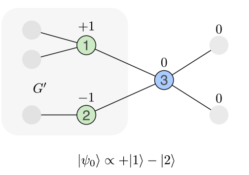
(a)

(b)

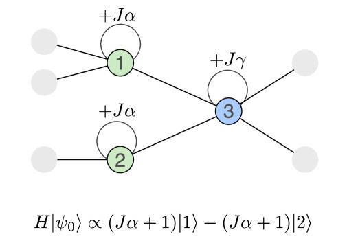
(c)

Figure 7: Schematic illustration of the impact of self-loops on eigenvectors. (a) Consider a Fock space graph without self-loops, where $\ket{\psi_{0}}$ is an eigenstate exhibiting an interference zero at $\ket{3}$. As a result, $\ket{\psi_{0}}$ is caged on the subgraph $G^{\prime}$, with other vertices shown in gray or omitted for clarity. For simplicity, all edges are uniformly weighted by $+1$. The detailed graph structure of $G^{\prime}$ is not crucial here and serves only as a schematic representation, provided that $\ket{\psi_{0}}$ can manifest as an eigenstate. (b) In general, introducing generically weighted self-loops disrupts $\ket{\psi_{0}}$, making it no longer an eigenstate. (c) However, if the vertices $\ket{1}$ and $\ket{2}$ are both assigned self-loops with equal weight $+U\alpha$, distinct from the self-loop weight of $\ket{3}$, a cancellation at $\ket{3}$ can still occur, while preserving $\ket{\psi_{0}}$ as an eigenstate. In this case, the eigenenergy is shifted by $U\alpha$ compared to (a). This phenomenon, which emerges from non-uniform self-loops across the entire graph and imposes structure (or order) within disorder, is referred to as order-by-disorder in the Hilbert space.

Up to this point, we have focused on the topological structure of the Fock space graph defined solely by $\widehat{O}_{\text{kin}}$, while temporarily neglecting the effects of $\widehat{O}_{\text{pot}}$, which manifest as weighted self-loops on the Fock space graph. Once $\widehat{O}_{\text{pot}}$ is included, it can introduce non-trivial effects on the possible cancellations. In general, $\widehat{O}_{\text{pot}}$ mixes the eigenstates of $\widehat{O}_{\text{kin}}$, disrupting the ICQMBS discussed earlier. However, not all ICQMBS are destroyed by $\widehat{O}_{\text{pot}}$. Some can persist under non-uniformly weighted self-loops. This phenomenon, referred to as order-by-disorder in the Hilbert space (OBDHS), will be the primary focus of this section.

The OBDHS mechanism resembles the destructive interference discussed in the underlying Fock space graph without self-loops, providing a clear topological explanation. As shown in Fig. 7c, the self-loops, though non-uniformly weighted across the entire Fock space graph, are chosen to have equal weights on a finite support, forming a subgraph $G^{\prime}$. When neglecting the self-loops, this subgraph features interference zeros around its outer boundary, allowing the formation of caged eigenstates. When uniformly weighted self-loops are applied to this subgraph, they lift the energy of ICQMBS by a constant value while preserving these states as eigenstates. The self-loop weights on the rest of the Fock space graph can be assigned arbitrarily, as they act only on interference zeros and do not affect the eigenstates. Consequently, the addition of self-loops functions as a selector of basis states, allowing ICQMBS to persist as eigenstates even under non-uniformly weighted self-loops. These eigenstates experience a uniform increase in eigenenergy, while other states are no longer eigenstates.

It should not be surprising that OBDHS depends on how the self-loop weights are assigned. For simplicity, we begin by considering a Hamiltonian of the form $\widehat{H}=\widehat{O}_{\text{kin}}+\widehat{O}_{\text{pot}}(\left\{U_{i}\right\})=\widehat{O}_{\text{kin}}+U\widehat{O}_{\text{pot}}$, where $U$ is the only tunable parameter uniformly applied to each lattice site. Extending the same idea to a general set of parameters $\{U_{i}\}$ is straightforward. As illustrated in Fig. 7c, the uniform self-loop weights within the subgraph $G^{\prime}$ are expressed as $U\alpha$, where $\alpha$ is typically tied to the detailed properties of the basis states, independent to the value of $U$. For instance, in the 1D spin-1 XY model, the $D$ term counts for the number of non-magnons in a basis state (see Sec. V). This introduces an order amidst the non-uniformly weighted self-loops (disorder), thus is referred to as order-by-disorder in the Hilbert space. In later sections, we will provide more concrete examples using two lattice models. For now, we outline a few general properties of the OBDHS mechanism:

1. This process does not require $\widehat{O}_{\text{kin}}$ and $\widehat{O}_{\text{pot}}$ to commute.

2. For a Hamiltonian $\widehat{H}=\widehat{O}_{\text{kin}}+U\widehat{O}_{\text{pot}}$, ICQMBS are characterized by $\expectationvalue{\widehat{O}_{\text{kin}}}=p$ and $\expectationvalue{\widehat{O}_{\text{pot}}}=\alpha$, where $U\alpha$ is the self-loop weight on the subgraph $G^{\prime}$ hosting ICQMBS, and $p$ is the eigenvalue of ICQMBS on the underlying subgraph (not necessarily zero). Notably, $p$ and $\alpha$ are independent of the value of $U$, and the eigenenergy of ICQMBS is given by $p+U\alpha$.

3. The eigenvector of the ICQMBS remains unchanged as the value of $U$ is varied. In this sense, it is distinct from the neighboring extended eigenstates, even though the level spacing is exponentially small, thereby violating ETH.

Let us examine the role of $\widehat{O}_{\text{pot}}$ more closely. The self-loops effectively repeat the wavefunction weight $c_{i}$ at vertex $v_{i}$, scaled by the weight of the self-loop $A_{v_{i},v_{i}}$, constructively interfering with the state. The redistributed weight $\tilde{c_{i}}$ at vertex $v_{i}$ through $A$ is therefore given by

$$\tilde{c_{i}}\coloneqq A_{v_{i},v_{i}}c_{i}+\sum_{v_{j}\in\partial v_{i}}A_{v_{i},v_{j}}c_{j}\text{.}$$ (17)

In general, achieving an interference zero $\tilde{c_{i}}=0$ requires all terms in Eq. 17 to cancel out. However, for the state to remain an eigenstate while maintaining a finite energy density, it must satisfy $\tilde{c_{i}}=\omega c_{i}$ for some generally non-zero eigenvalue $\omega$, to remain at finite energy density. This is only possible when $c_{i}=0$. Then, Eq. 17 resembles a typical interference zero with clear topological meaning.

The challenge now lies in determining whether the rest of the nonzero weights $c_{i}$ on $G^{\prime}$ can form an eigenstate. Specifically, the condition is whether $\tilde{c_{i}}=\omega c_{i}$ holds for some generally non-zero eigenvalue $\omega$ across all vertices in $G^{\prime}$ with $c_{i}\neq 0$. Equivalently, the ratio $\tilde{c_{i}}/c_{i}$ should be constant for all such vertices:

$$\tilde{c_{i}}/c_{i}=A_{v_{i},v_{i}}+\sum_{v_{j}\in\partial v_{i}}A_{v_{i},v_{j}}\frac{c_{j}}{c_{i}}\text{.}$$ (18)

For this equality to hold with a constant right-hand side, both terms must be constant across all relevant vertices . This observation already suggests that the self-loop weights $A_{v_{i},v_{i}}$ should be equal for all vertices in $G^{\prime}$. The second term on the right-hand side of Eq. 18 can also be made constant through various mechanisms. Below, we outline a few special cases based on the lattice models we have studied:

1. Consider a bipartite graph $G=\{V_{b},V_{w},E\}$ where the non-zero coefficients $c_{i}$ are localized within one bipartite subset $U$, so $G^{\prime}=\{V_{b}\}$. In this case, for any $v_{i}\in V_{b}$, all neighboring vertices $v_{j}\in\partial v_{i}$ belong to the opposite subset $V_{w}$ and have $c_{j}=0$. Therefore, the sum is simplified to $\sum_{v_{j}\in\partial v_{i}}A_{v_{i},v_{j}}c_{j}/c_{i}=0$. Consequently, ICQMBS are characterized by $\expectationvalue{\widehat{O}_{\text{kin}}}=0$ and a constant value of $\expectationvalue{\widehat{O}_{\text{pot}}}$ set by self-loops.

2. Suppose the graph $G$ is unweighted, so $A_{v_{i},v_{j}}=1$ for all $v_{i}\neq v_{j}$, and the subgraph $G^{\prime}$ has a constant vertex degree $d$, meaning $\text{deg}(v_{i})=d$ for all $v_{i}\in G^{\prime}$. The self-loops are uniformly weighted by $Ud$ within $G^{\prime}$. In many cases, the ratio $c_{j}/c_{i}$ become identical across all vertices in $G^{\prime}$, resulting in $\sum_{v_{j}\in\partial v_{i}}c_{j}/c_{i}\sim\kappa d$, where $\kappa$ is a proportionality factor satisfying $0<\kappa<1$ because not all $d$ neighbors of $v_{i}$ are within $G^{\prime}$. As a result, $\expectationvalue{\widehat{O}_{\text{kin}}}=\kappa d$ and $\expectationvalue{\widehat{O}_{\text{pot}}}=d$ are two distinct and non-zero constants.

It is important to note that additional cases exist beyond these two, as long as the states are eigenstates surrounded by interference zeros and the self-loops on the support of ICQMBS are uniformly weighted, thereby enabling the OBDHS mechanism.

Lastly, we comment that while models with non-uniformly weighted self-loops are more complex, gaining a deeper understanding of self-loops could provide insights into the study of MBL, another ETH-violating mechanism. From a graph theory perspective, MBL can be roughly interpreted as a competition between hopping on vertices and returning to them via randomly weighted self-loops (i.e., disorder), which leads to localization on individual vertices. Unfortunately, a comprehensive analytical tool for handling generically weighted self-loops is still lacking.

V QMBS in 1D spin-1 XY model

In the following sections, we apply the graph-based method to two lattice models: the 1D spin-1 XY model and the 2D $U(1)$ LGTs. The Fock space graphs of these models are primarily bipartite, with only a few exceptions depending on the boundary conditions, which will be discussed separately.

We begin with the 1D spin-1 XY model, which is unconstrained, making it easier to identify cancellations between the two bipartite subsets caused by local operators. In the following Sec. V.1, we will review the two types of ICQMBS that have been analytically constructed via quasi-particle picture in [75, 30]. We will demonstrate how these ICQMBS are caged within their respective bipartite subsets and how graph-based analysis aids in understanding the destructive interference responsible for their caging structure.

We then extend the Fock space graph formalism to the 2D $U(1)$ LGT models in the next section. However, due to their gauge-constrained nature, deriving analytical expressions is challenging. Instead, we will employ the searching protocol discussed in Sections III.3.2 and III.3.3 for the numerical search of ICQMBS.

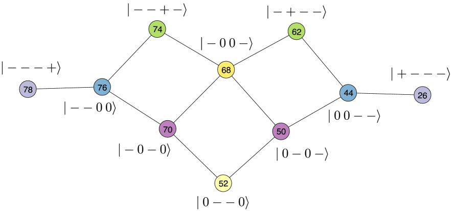
(a)

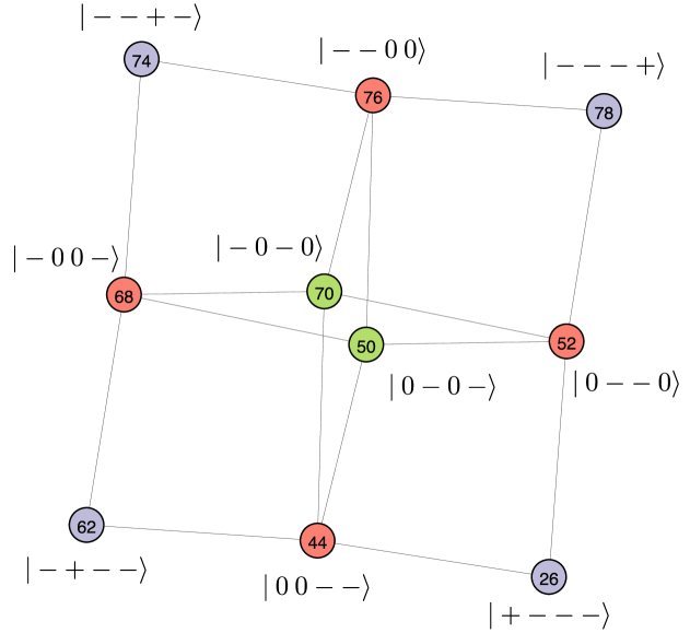
(b)

Figure 8: Graph representation of the $S^{z}=-2$ sector for a lattice of size $L=4$ under (a) OBC and (b) PBC. Both graphs are bipartite, with self-loops omitted for clarity. Vertices are colored according to their automorphism orbits, and each label indicates the corresponding $i$-th basis state. The spin configuration of each basis state is shown alongside to demonstrate the quasi-particle structure. Here, we use the labeling scheme outlined in Appendix A for the vertex label $i$.

V.1 1D spin-1 XY model and the important symmetries

We begin with the 1D spin-1 lattice of length $L$ with both the open boundary (OBC) and periodic boundary conditions (PBC). The spin-1 XY model is described by the Hamiltonian [75],

$$\widehat{H}_{\text{XY}} =\widehat{O}_{\text{kin}}+\widehat{O}_{\text{pot}}\text{,}$$ (19)

$$\widehat{O}_{\text{kin}} =J\sum_{r}(S_{r}^{+}S_{r+1}^{-}+S_{r}^{-}S_{r+1}^{+})\text{,}$$

$$\widehat{O}_{\text{pot}}(\left\{U_{i}\right\}) =h\sum_{r}S_{r}^{z}+D\sum_{r}(S_{r}^{z})^{2}\text{,}$$

where $r=1,\dots,L$ labels lattice sites. The operators $S_{r}^{\alpha}$ ($\alpha=x,y,z$) are spin-1 operators, and the ladder operators $S_{r}^{\pm}=S_{r}^{x}\pm iS_{r}^{y}$ are defined as usual. We have also cast the Hamiltonian into $\widehat{O}_{\text{kin}}$ and $\widehat{O}_{\text{pot}}$ by working with the standard $S^{z}$ basis. For OBC, the sum for the $J$-hopping term runs up to $r=L-1$, while for PBC, an additional term connects site $L$ back to site $1$. For clarity in the later discussion, conventionally, the spin configuration $\ket{+}$ is referred to as a bimagnon (a doubly-raised spin), in contrast to a magnon $\ket{0}$, both of which represent excitations from the vacuum state $\ket{-}$.

We aim to demonstrate that ICQMBSs emerge solely from the topological structure of the Fock space graph, independent of any symmetries of the Hamiltonian. To achieve this, we have included the term $\widehat{H}_{D}=D\sum_{r}(S_{r}^{z})^{2}$ in $\widehat{O}_{\text{pot}}$, ensuring that $\widehat{O}_{\text{kin}}$ and $\widehat{O}_{\text{pot}}$ do not commute for any nonzero $D$. Furthermore, as noted in [131], the Hamiltonian $\widehat{H}_{\text{XY}}$ possesses a non-local $\text{SU}(2)$ symmetry in 1D. We can introduce a third-neighbor hopping term, $\widehat{H}_{3}=J_{3}\sum_{r}(S_{r}^{+}S_{r+3}^{-}+\text{h.c.})$, to destroy this symmetry. As we will demonstrate, even when both $\widehat{H}_{D}$ and $\widehat{H}_{3}$ are included, ICQMBS can still exist, although their wavefunctions may differ from those arising solely when both $\widehat{H}_{D}$ and $\widehat{H}_{3}$ are absent.

Nonetheless, this model exhibits total $S^{z}$ symmetry, ensured by the operator $S^{z}=\sum_{r}S_{r}^{z}$, which commutes with the Hamiltonian, i.e., $[\widehat{H}_{\text{XY}},S^{z}]=0$. In the computational ($S^{z}$) basis, this symmetry splits the graph into disconnected subgraphs $G_{S^{z}}$, each corresponding to a specific $S^{z}$ sector. Within the $G_{S^{z}}$, each vertex has a self-loop with a uniform weight of $hS^{z}$ across all vertices in that subgraph. Additionally, there is a non-uniform contribution from $D$, depending on the number of non-magnons on a corresponding product state basis. For instance, the state $\ket{++-0}$ has a self-loop weighted by $h+3D$. The $S^{z}$ symmetry also guarantees two exact eigenstates that are fully polarized, $\ket{\Omega}=\bigotimes_{r=1}^{L}\ket{-}_{r}$ and $\ket{\Omega^{\prime}}=\bigotimes_{r=1}^{L}\ket{+}_{r}$. These eigenstates correspond to two isolated vertices, are annihilated by $\widehat{O}_{\text{kin}}$ due to their disconnected nature, and have eigenvalues $(\pm h+D)L$, determined solely by the self-loop.

Additionally, the kinetic term $\widehat{O}_{\text{kin}}$ may exhibit spectral reflection symmetry about zero energy depending on the boundary conditions. This symmetry is generated by the parity operator

$$\widehat{C}=\exp{\pm i\pi\sum_{r\in\text{e/o}}S_{r}^{z}}\text{,}$$ (20)

where the sum is taken over either even lattice sites (with a positive phase) or odd lattice sites (with a negative phase). Importantly, both the phase ($\pm i\pi$) and the sum over even or odd lattice sites are matters of choice, provided that the choice is consistent. Specifically, for different boundary conditions, we find that ^,:

• OBC: The spectral reflection symmetry is ensured by $\widehat{C}$, and $\{\widehat{O}_{\text{kin}},\widehat{C}\}=0$ for any $L$.

• PBC: The operator $\widehat{C}$ is ill-defined when $L$ is odd because the distinction between even and odd sites becomes ambiguous under periodic boundary conditions. However, if $L$ is even, we still have $\{\widehat{O}_{\text{kin}},\widehat{C}\}=0$.

Consequently, the Hamiltonian $\widehat{H}_{\text{XY}}$ decomposes into disconnected bipartite subgraphs $G_{S^{z}}$, except for odd $L$ under PBC, which requires special consideration (see Appendix C). The bipartite nature of $G_{S^{z}}$ immediately suggests QMBS localized in the two bipartite subsets, as discussed in Sec. III.3.3. These QMBS are annihilated by the kinetic operator $\widehat{O}_{\text{kin}}$, i.e., $\widehat{O}_{\text{kin}}\ket{\psi_{\text{scar}}}=0$. We first consider the case $D=0$. Then, the energy eigenvalues of these QMBS are solely determined by the $h$-potential term, $E_{n}=h(-L+n)$, where $n=0,1,\dots,L$. As these QMBS have equally spaced eigenvalues in the spectrum, they are referred to as the tower of scars. For $D\neq 0$, the interference-caged condition becomes more intricate. Nevertheless, we will demonstrate that a tower of scars denoted $\ket{\mathcal{S}_{n}}$ persists, consisting of basis states with the same number of $\ket{+}$ spins (bimagnons) inserted into the background state $\ket{\Omega}$, with no $\ket{0}$ spins (magnons) present. This is, therefore, referred to as the order-by-disorder in the Hilbert space, where the "order" is introduced by $\widehat{H}_{D}$. Consequently, the energies of these states are given by $E_{n}=h(-L+2n)+DL$, resulting in an energy increment of two between successive states in the tower.

The search for QMBS now reduces to identifying the zero-energy eigenstates of $\widehat{O}_{\text{kin}}$ within each $S^{z}$ sector. Since the spin-1 XY model is unconstrained and defined in one dimension, identifying the local operators responsible for the destructive interference becomes straightforward, leading to a quasi-particle description and the corresponding algebraic structure. In the following sections, we review two types of QMBS that were analytically constructed in [75, 30], with a focus on how destructive interference manifests in the graph. Specifically, we examine two sets of QMBS within the bipartite subsets, denoted $\ket{\mathcal{S}_{n}}$ and $\ket{\mathcal{S}^{\prime}_{n}}$, where $n=0,\dots,L$ and $S^{z}=-L+2n$, representing the towers of scars. These scars exhibit an increment of 2 in $S^{z}$ within the tower, due to the quasi-particles used in their construction. However, this increment is not strictly necessary, as QMBS can also exist in $S^{z}$ sectors with single-step increments above $-L$, as we will discuss later. Additionally, $\ket{\mathcal{S}_{n}}$ persists under both $D\neq 0$ and $J_{3}\neq 0$, while $\ket{\mathcal{S}^{\prime}_{n}}$ only exists under $D=0$, and takes different wavefunction form when introducing non-zero $J_{3}$.

At this stage, we also comment that the term $\widehat{H}_{3}$ can be generalized to any odd-neighbor hopping while preserving the bipartite structure of $G_{S^{z}}$, provided that $\anticommutator{\widehat{O}_{\text{kin}}}{\widehat{C}}=0$ in the respective boundary conditions, except for odd $L$ under PBC. Moreover, since $\widehat{H}_{3}$ (and any odd-neighbor hopping) also commute with the total $S^{z}$, i.e., $\commutator{\widehat{H}_{3}}{S^{z}}=0$, these additional quantum processes, represented by graph edges, alter the topology within each subgraph $G_{S^{z}}$ without connecting different subgraphs. Consequently, each $G_{S^{z}}$ remains bipartite. We will discuss how these additional graph edges affect the wave function of ICQMBS.

V.1.1 Quasi-particle description of $\ket{\mathcal{S}_{n}}$

We first consider the case where $J_{3}=0$. The local kinetic term $h_{r,r+1}^{\text{kin}}=S_{r}^{+}S_{r+1}^{-}+S_{r}^{-}S_{r+1}^{+}$ acts on the two-site states as follows:

$$h_{r,r+1}^{\text{kin}}\ket{\pm 0} =\ket{0\pm}\text{,}$$ (21)

$$h_{r,r+1}^{\text{kin}}\ket{0\pm} =\ket{\pm 0}\text{,}$$

which effectively swaps the positions of $\ket{0}$ and $\ket{\pm}$. More importantly, we also have:

$$h_{r,r+1}^{\text{kin}}\ket{--} =h_{r,r+1}^{\text{kin}}\ket{++}=0\text{,}$$ (22)

$$h_{r,r+1}^{\text{kin}}\ket{+-} =h_{r,r+1}^{\text{kin}}\ket{-+}=\ket{00}\text{.}$$

This shows that the operator annihilates fully polarized states $\ket{--}$ and $\ket{++}$, while transforming $\ket{+-}$ and $\ket{-+}$ into $\ket{00}$.

We can generalize the two-site case to larger systems by joining more spins on both sides, regardless of different boundary conditions. Consider two many-body basis states, $\ket{\cdots+_{r}-_{r+1}\cdots}$ and $\ket{\cdots-_{r}+_{r+1}\cdots}$, which differ only at sites $r$ and $r+1$. These two bases belong to the same bipartite subset, as guaranteed by the parity operator $\widehat{C}$, and can cancel out at $\ket{\cdots 0_{r}0_{r+1}\cdots}$ by choosing opposite signs, yielding

$$h_{r,r+1}^{\text{kin}}\Bigl{(}\ket{\cdots+_{r}-_{r+1}\cdots}-\ket{\cdots-_{r}+_{r+1}\cdots}\Bigr{)}=0\text{.}$$ (23)

This cancellation is frustration-free and can always occur unless the two basis states $\ket{\cdots+_{r}-_{r+1}\cdots}$ and $\ket{\cdots-_{r}+_{r+1}\cdots}$ are not present in the corresponding $S^{z}$ sector.

Moreover, the destructive interference in Eq. 23 suggests that QMBS in each $S^{z}$ sector, with increments of 2, can be constructed by the insertion or removal of bimagnons into the lattice. Specifically, as shown analytically in [75], these QMBS can be expressed as

$$\ket{\mathcal{S}_{n}}=\mathcal{N}(n)(J^{+})^{n}\ket{\Omega}\text{,}$$ (24)

where $n=0,\cdots,L$ represents the number of inserted bimagnons, $\ket{\Omega}=\bigotimes_{r}\ket{-}_{r}$ is the fully polarized vacuum state, and $\mathcal{N}(n)=\binom{L}{n}^{-\frac{1}{2}}=\sqrt{\frac{(L-n)!n!}{L!}}$ are normalization factors. The operators $J^{\pm}$, which insert or remove a bimagnon of momentum $\pi$ into the target state, are given by

$$J^{\pm}=\frac{1}{2}\sum_{r=1}^{L}e^{i\pi r}(S_{r}^{\pm})^{2}\text{,}$$ (25)

where the lattice translation effectively relates the basis states with the same number of inserted bimagnons, and the Fourier coefficient $e^{i\pi r}$ determines the appropriate sign for cancellation, which alternates between $\pm 1$ for momentum $\pi$. Hence, the tower $\ket{\mathcal{S}_{n}}$ is sometimes referred to as the $\pi$-bimagnon scars.

Notably, these scar eigenstates are related by an emergent $SU(2)$ algebra (distinct from that of [131]), generated by the ladder operators $J^{\pm}$ and $J^{z}=\frac{1}{2}\sum_{r}S_{r}^{z}=\frac{1}{2}S^{z}$, with the commutation relations:

$$\left[J^{+},J^{-}\right]=2J^{z}\text{; }\left[J^{z},J^{\pm}\right]=\pm J^{\pm}\text{.}$$ (26)

This structure is known as the spectrum-generating algebra (SGA) for the tower of scars [30]. In graph terms, it arises directly from the bipartite nature of each $S^{z}$ sector, supporting the frustration-free zero-energy states. The addition of weighted self-loops lifts these zero-energy states into a tower. Since the involved basis states consist only of the insertion of bimagnons, this energy lifting within each $G_{S^{z}}$ is given by $hS^{z}+DL$, resulting in equally spaced energy levels.

Now, let’s consider the case where $\widehat{H}_{3}$ is included. Similarly, the cancellation pattern follows the same as that in Eq. 23, with $r+1$ replaced by $r+3$. These additional cancellations remain confined to basis states described by the insertion of $n$ bimagnons, so other vertices in the graph are unaffected. However, the newly introduced quantum process does add edges to vertices with $n$ bimagnons, as illustrated in Fig. 9b. We claim that these new edges do not alter the original sign choice of the wavefunction weights in $\ket{\mathcal{S}_{n}}$. This is because the two basis states $\ket{\cdots+_{r}-_{r+1}\cdots}$ and $\ket{\cdots-_{r}+_{r+1}\cdots}$, where a bimagnon is shifted by one position, must carry opposite signs to achieve cancellation, as seen in Eq. 23. This observation can be extended to any two basis states $\ket{\cdots+_{r}\cdots-_{r^{\prime}}\cdots}$ and $\ket{\cdots-_{r}\cdots+_{r^{\prime}}\cdots}$, where the bimagnon is shifted by an odd number of position ($|r-r^{\prime}|$ is odd), ensuring that the two states still carry opposite signs. Consequently, $\ket{\mathcal{S}_{n}}$ remains the same, even through the non-local $\text{SU}(2)$ symmetry is broken by $\widehat{H}_{3}$ (or any other odd-neighbor hopping).

Lastly, as shown in Fig. 8a and 8b, the two graphs $G_{S^{z}=-2}$ for a lattice of size $L=4$ are depicted under both OBC and PBC. The destructive interference arising from their bipartite nature is evident in both figures for the basis states involved in $\ket{\mathcal{S}_{n=1}}$. However, while the basis states containing a bimagnon are sufficient to form a QMBS, for $D=0$, two additional states, $\ket{-0-0}$ and $\ket{0-0-}$, can also contribute to the QMBS under both boundary conditions. This suggests a possible generalization of $\ket{\mathcal{S}_{n}}$ when $D=0$: by inserting either a bimagnon or a pair of magnons on the even or odd sublattice. Specifically, we promote the doubly raising operator $(S_{r}^{+})^{2}$ into $(S_{r}^{+})(S_{r^{\prime}}^{+})$, with $r$ and $r^{\prime}$ being both even or odd, such that the state remains in the same bipartite subset. When $r=r^{\prime}$, this recovers the original expression for creating a bimagnon. However, the precise choice of wavefunction weights depends on the boundary conditions, as seen in Fig. 8a and 8b. Moreover, this construction would sacrifice the frustration-free property and increase the entanglement entropy as it involves more vertices. On the other hand, introducing a non-zero $D$ prevents this type of cancellation and restricts interference to states containing $n$-bimagnons. This is, therefore, an example of the order-by-disorder in the Hilbert space, introduced by $\widehat{H}_{D}$.

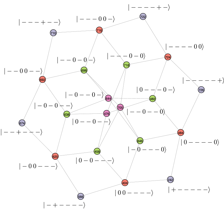
(a)

(b)

Figure 9: Graph representation of the $S^{z}=-4$ sector for a lattice of size $L=6$ under PBC: (a) without $\widehat{H}_{3}$ and (b) with $\widehat{H}_{3}$. Both graphs are bipartite, with self-loops omitted for clarity. Vertices are colored according to their automorphism orbits, and each label indicates the corresponding $i$-th basis state. The spin configuration of each basis state is shown alongside to demonstrate the quasi-particle structure. In panel (b), the introduction of $\widehat{H}_{3}$ converts the rose (black•) vertices in (a) into the red (black•) automorphism orbit. For clarity, only a subset of the newly added edges is shown with dashed lines. Specifically, vertices 698, 700, and 724, representing the green (black•), rose (black•), and red (black•) orbits in panel (a), are chosen as examples. The remaining omitted edges can be inferred by automorphism symmetry.

V.1.2 Quasi-particle description of $\ket{\mathcal{S}^{\prime}_{n}}$

In addition to the tower of scars $\ket{\mathcal{S}_{n}}$, there exists another tower of scars $\ket{\mathcal{S}^{\prime}_{n}}$ orthogonal to $\ket{\mathcal{S}_{n}}$. However, unlike $\ket{\mathcal{S}_{n}}$, the scars $\ket{\mathcal{S}^{\prime}_{n}}$ are not frustration-free eigenstates of $\widehat{O}_{\text{kin}}$, and only exist under PBC (and even $L$) with $D=0$. Furthermore, their expressions change in the presence of $\widehat{H}_{3}$, necessitating separate consideration.

We begin by considering the case without the inclusion of $\widehat{H}_{3}$, these states are identified as [75]:

$$\ket{\mathcal{S}^{\prime}_{n}} =\mathcal{N}(n)\sum_{r_{1}\neq r_{2}\neq\cdots\neq r_{n}}(-1)^{r_{1}+\cdots+r_{n}}(S_{r_{1}}^{+}S_{r_{1}+1}^{+})$$ (27)

$$\quad\times(S_{r_{2}}^{+}S_{r_{2}+1}^{+})\cdots(S_{r_{n}}^{+}S_{r_{n}+1}^{+})\ket{\Omega}\text{,}$$

where the normalization factors $\mathcal{N}(n)$ follow the same binomial form as in Eq. 24. In particular, the operator $S_{r}^{+}S_{r+1}^{+}$ inserts a pair of adjacent magnons (referred to as a bond-bimagnon in [75]) into the fully polarized background $\ket{\Omega}$, incrementing $S^{z}$ by 2. Notably, two bond-bimagnons can have finite overlap at one site to create states like $\ket{\cdots 0+0\cdots}$. As ensured by the parity operator $\widehat{C}$, basis states containing the same number of bond-bimagnons, such as $\ket{\cdots 0000\cdots}$ or $\ket{\cdots 0+0-\cdots}$, must belong to the same bipartite subset.

Without analytically deriving the scars $\ket{\mathcal{S}^{\prime}_{n}}$, which are annihilated by $\widehat{O}_{\text{kin}}$ but not frustration-free, we demonstrate the cancellation mechanism in Fig. 8b. The red (black•) vertices represent the four basis states that contain a bond-bimagnon, with wavefunction amplitudes of $\pm 1$ assigned as shown in Eq. 27, ensuring that they cancel out in the opposite bipartite subset. This cancellation involves all edges, indicating it is not frustration-free. Readers are encouraged to examine the local operators connecting the vertices, where each edge corresponds to an operator of the form $S_{r}^{+}S_{r^{\prime}}^{-}$ (or $S_{r}^{-}S_{r^{\prime}}^{+}$) for all possible neighboring pairs of $r$ and $r^{\prime}$.

The existence of these QMBS under PBC, but not OBC, is also illustrated in Fig. 8. Under OBC, when a basis state contains a bimagnon at either end of the lattice, such as $\ket{+-\cdots-}$, it can only connect to $\ket{00-\cdots-}$ through spin flips. However, it cannot connect to $\ket{0-\cdots-0}$, a connection that is only possible under PBC. As a result, the destructive interference needed for the formation of bond-bimagnon QMBS cannot occur under OBC.

Furthermore, in the presence of $\widehat{H}_{D}$, non-uniform weights are introduced to the self-loops. This does not affect the one-bond-bimagnon state $\ket{\mathcal{S}^{\prime}_{1}}$. However, for states with multiple bond-bimagnons, such as those shown in Fig. 10, the two states $\ket{0000}$ and $\ket{0+0-}$ are assigned self-loop weights of $0$ and $2D$, respectively. Consequently, the tower of scars is destroyed for all $n>1$.

When $\widehat{H}_{3}$ is included, states with two magnons separated by three sites, such as $\ket{\cdots 0_{r}--0_{r+3}\cdots}$, begin to contribute to the cancellation process. We refer to these states as third-neighbor bimagnon states. Notably, under PBC with even $L$, the graph remains bipartite, as guaranteed by the operator $\widehat{C}$. As illustrated in Fig. 9b, third-neighbor bimagnon states are incorporated into the same automorphism orbit as the bond-bimagnon states. Numerical studies indicate that QMBS can localize within the bipartite subset formed by third-neighbor bimagnon and bond-bimagnon states, albeit with a more complex choice of wavefunction weights. Consequently, the wavefunction expression deviates from $\ket{\mathcal{S}^{\prime}_{n}}$ in Eq. 27. However, we could not identify a closed-form expression due to its complexity. Furthermore, these QMBS can only remain as eigenstates under $D\neq 0$ when $n=1$, as the basis states containing $n$ bond-bimagnons or third-neighbor bimagnons may exhibit finite overlaps.

V.1.3 QMBS beyond $\ket{\mathcal{S}_{n}}$ and $\ket{\mathcal{S}^{\prime}_{n}}$

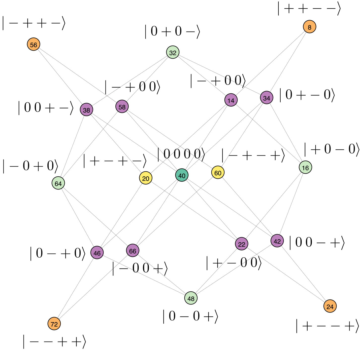
Figure 10: Graph representation of the $S^{z}=0$ sector for a lattice of size $L=4$ under PBC. This graph is bipartite, with self-loops omitted for clarity. Vertices are colored according to their automorphism orbits, and each label indicates the corresponding $i$-th basis state. The spin configuration of each basis state is shown alongside to demonstrate the quasi-particle structure.

As discussed in the previous two sections, viewing the Hilbert space as a Fock space graph reveals a rich combinatorial structure, often interpreted through the quasi-particle framework. As a result, generic QMBS typically consist of multiple types of quasi-particles arranged in a combinatorial fashion, as long as they are annihilated by $\widehat{O}_{\text{kin}}$. As illustrated in Fig. 10, two types of quasi-particles, bimagnons and bond-bimagnons, are present in such a combinatorial arrangement. In this figure, the purple (black•) vertices represent basis states where both the bimagnon $\ket{+}$ and the bond-bimagnon $\ket{00}$ are inserted into the background state $\ket{\Omega}$, forming QMBS within this bipartite subset. The analytical expression for this QMBS resembles Eq. 27, with the distinction that one of the bond-bimagnons excited by $S_{r}^{+}S_{r+1}^{+}$ is replaced by $(S_{r}^{+})^{2}$, which excites a bimagnon. Because of the highly combinatorial nature of these states, expressing them in closed form is more challenging for generic $L$ compared to those composed purely of bimagnons or bond-bimagnons.

In contrast, the orange (black•) and yellow (black•) vertices in the opposite bipartite subset (in Fig. 10) correspond to basis states involving only bimagnons, forming $\ket{\mathcal{S}_{n=2}}$. Interestingly, the orange (black•) and turquoise (black•, i.e., $\ket{0000}$) vertices also establish a valid cancellation. Additionally, the pale-green (black•) and turquoise (black•) vertices, which contain bond-bimagnons, form another tower $\ket{\mathcal{S}^{\prime}_{n=2}}$. It is worth noting that all three cancellation mechanisms (in this bipartite subset) fall under the scope of Lemma III.2, while the purple (black•) vertices are localized as described by Lemma III.1.

However, most of these anomalous states are not robust against the symmetry breaking introduced by $H_{D}$ and $H_{3}$. As summarized in Table 1, only a few anomalous states—aside from the tower of scars $\ket{S_{n}}$, highlighted in gray—persist as QMBS even when the $\text{SU}(2)$ symmetry [131] is broken by $H_{3}$. These QMBS are scarce in the presence of $H_{3}$ but more abundant when $H_{3}$ is absent. While the nature of these QMBS remains not fully understood in general, we report a few notable cases based on our numerical findings. When $H_{3}$ is absent, the QMBS in the $S^{z}=-L+1$ sector is not a product state but rather a low-entangled state. These QMBS arise from the insertion of individual magnon $\ket{0}$. To illustrate this, let’s examine the $S^{z}=-3$ sector on a lattice of size $L=4$ under PBC, which forms a $C_{4}$ graph. Specifically, we can show that

$$\widehat{O}_{\text{kin}}\left(\ket{0---}-\ket{--0-}\right)=0\text{,}$$ (28)

where the two basis states cancel out at $\ket{---0}$ and $\ket{-0--}$ (and conversely, these can also cancel at $\ket{0---}$ and $\ket{--0-}$). In fact, all $S^{z}=-L+1$ sectors persist as a cycle graph $C_{L}$ for all even $L$ under PBC. However, cancellation leading to QMBS formation is only possible when $L$ is a multiple of four. In the case of OBC, a similar insertion of individual magnon is also observed in the $S^{z}=-L+1$ sector, forming path graph $P_{L}$. Unlike the case in PBC, where both bipartite subsets can form a valid cancellation, in OBC, only one subset can form QMBS.

We also compared ED with our algorithm by analyzing the null space of the bipartite graphs, as summarized in Table 1. The consistent results indicate that our method provides a novel perspective based on destructive interference in the Fock space graph—a viewpoint not previously discussed. The spin-1 XY model serves as a simple toy example to illustrate this concept. In the next section, we will apply the same idea to more complex 2D models with gauge constraints.

To date, we have shown how orbit-based analysis helps explain the destructive interference responsible for the localization of QMBS. In 1D systems, it is often possible to identify the quasi-particles associated with these orbits. However, since these orbits manifest as highly combinatorial structures, examining them remains a challenging task in the thermodynamic limit $L\to\infty$. Before concluding this section, we summarize in Table 1 the number of QMBS found numerically in the spin-1 XY model. These results were obtained using the search protocol described in Sec. III.3.3 after filtering out vertices with identically weighted self-loops.

OBC
$L$	$S^{z}=0$	$S^{z}=\pm 1$	$S^{z}=\pm 2$	$S^{z}=\pm 3$	$S^{z}=\pm 4$	$S^{z}=\pm 5$	$S^{z}=\pm 6$	$S^{z}=\pm 7$	$S^{z}=\pm 8$
$4$	$1$	$0$	$1$	$0$	$1$	-	-	-	-
$5$	$0$	$1$	$0$	$1$	$1$	$1$	-	-	-
$6$	$1$	$0$	$1$	$0$	$1$	$0$	$1$	-	-
$7$	$0$	$1$	$0$	$1$	$0$	$1$	$1$	$1$	-
$8$	$1$	$0$	$1$	$0$	$1$	$0$	$1$	$0$	$1$
PBC
$L$	$S^{z}=0$	$S^{z}=\pm 1$	$S^{z}=\pm 2$	$S^{z}=\pm 3$	$S^{z}=\pm 4$	$S^{z}=\pm 5$	$S^{z}=\pm 6$	$S^{z}=\pm 7$	$S^{z}=\pm 8$
$4$	$5$	$2$	$3$	$2$	$1$	-	-	-	-
$5$	$1$	$0$	$0$	$0$	$0$	$1$	-	-	-
$6$	$5$	$0$	$3$	$0$	$3$	$0$	$1$	-	-
$7$	$0$	$0$	$0$	$0$	$0$	$0$	$0$	$1$	-
$8$	$1$	$0$	$1$	$0$	$4$	$0$	$5$	$2$	$1$

Table 1: Summary of the number of QMBS found in the 1D spin-1 XY model for various lattice sizes $L$ and boundary conditions, with both $D\neq 0$ and $J_{3}\neq 0$, across different $S^{z}$ sectors. A dash (-) signifies that the $S^{z}$ sector is not supported by the system size. The cells with a gray background indicate the tower of scars, $\ket{\mathcal{S}_{n}}$.

VI QMBS in QLM and QDM

Models with constrained Hilbert spaces have been widely studied as potential hosts for QMBS, such as the PXP model in both 1D and 2D [132, 133]. Another prominent example includes LGTs, which incorporate gauge constraints as local conditions. LGTs play a crucial role in both high-energy [134, 135] and condensed matter physics [106, 136, 137, 138]. In this section, we focus on matter-free $U(1)$ LGTs. Specifically, we explore QLM and QDM on the square lattice. These models share a common Hamiltonian, differing only in their choice of gauge constraints.

Unlike the previous section on the spin-1 XY model, identifying the relevant quasi-particles that can be annihilated by real space interference is significantly more challenging in constrained systems, especially in 2D, where the combinatorial structure is more complex. Instead, we rely on destructive interference of fictitious-particles as a guideline in the search for QMBS. Fortunately, the graphs induced in these two models remain bipartite under PBC, allowing us to apply the numerical search protocol discussed in Sec. III.3.3, with some model-specific adjustments. Notably, some of these fictitious-particles contribute to QMBS observed numerically in ED studies, referred to as lego scars in QDM [94] and sublattice scars in QLM [57].

We will review the studies of QMBS in the 2D QLM and QDM in Sec. VI.1. After properly defining the models and establishing the Fock space graph representation, we provide a short summary of the classification of QMBS. In Sec. VI.2, we will use ICQMBS to understand the previously unexplained Hilbert space order-by-disorder phenomena in numerical studies [56]. With the new insight from the Fock space graph picture of these models, we further use ICQMBS to understand the Type I QMBS from the topology perspective in Sec. VI.3. The Type I QMBS is an example of the topological ICQMBS, where the absolute robustness against the Fock space interference pattern preserving perturbations is a non-trivial many-body generalization from the single-particle case. In Sec. VI.4, we will discuss how our algorithm helps in the understanding of type-IIIA QMBS.

VI.1 $U(1)$ lattice gauge theories in 2D - quantum link and quantum dimer models

We will begin with an introduction to these two models in Sec. VI.1.1, followed by a review in Sec. VI.1.3 of several classes of QMBS investigated numerically through ED in previous studies [56, 94, 57]. We will then explain how the Fock space graph helps understand the destructive interference that localizes a subgraph eigenstate in these models, followed by an examination of the fictitious-particles that are annihilated at the outer boundary of these subgraphs.

VI.1.1 The definition of QLM and QDM

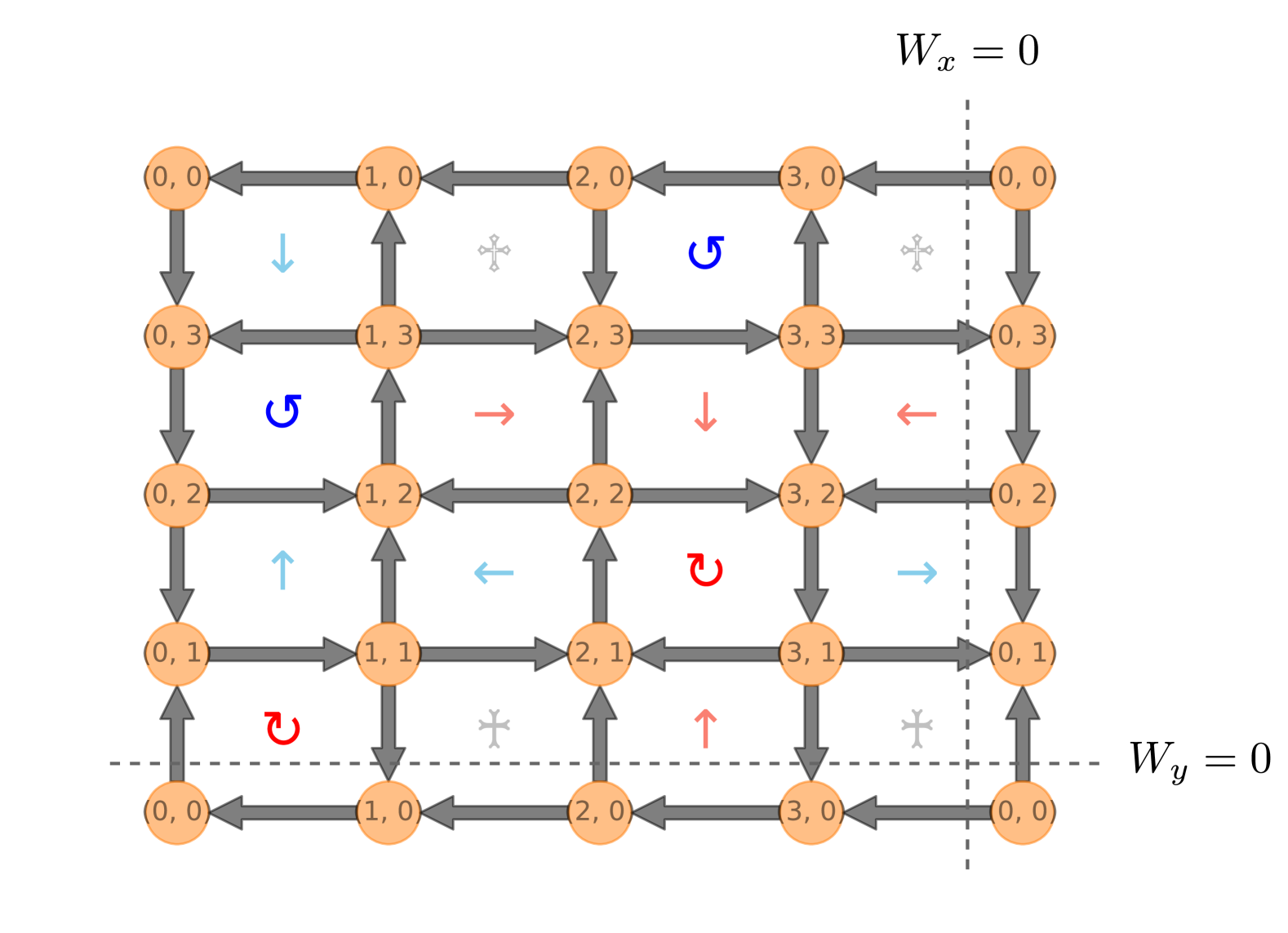
Figure 11: A lattice of size $(4,4)$ with periodic boundaries is shown. Each lattice site is labeled by its position $(x,y)$, with the origin conventionally placed at the lower-left corner (1st quadrant). For viewing convenience, the sites and links from the first column and row are repeated at the opposite boundary. Staggered charges of $\pm 1$ (as in QDM) are depicted, corresponding to either 1-in-3-out or 3-in-1-out configurations at each site. The dashed line represents the links contributing to the global flux $W_{\mu}$ in both directions, indicating the flux passing through the cross-section. For details on the colored symbols within each plaquette, refer to the main text.

The two models under consideration are defined on a two-dimensional square lattice of size $L_{x}\times L_{y}$ with periodic boundaries, as illustrated in Fig. 11. In this figure, each quantum link connecting two neighboring sites $\textbf{r}=(x,y)^{T}$ and $\textbf{r}+\hat{\mu}$ carries a spin-$1/2$ state, representing the elementary degrees of freedom, where $\hat{\mu}=\hat{x},\hat{y}$ denotes the two unit vectors on the square lattice. We follow the convention where upward and rightward arrows correspond to a spin-up state $\ket{\uparrow}$, while downward and leftward arrows correspond to a spin-down state $\ket{\downarrow}$. Additionally, on each link labeled by a tuple $(\textbf{r},\hat{\mu})$, the electric flux operator is defined as $E_{\textbf{r},\hat{\mu}}=S^{z}_{\textbf{r},\hat{\mu}}$, while the gauge fields are represented by the Pauli ladder operators, $U_{\textbf{r},\hat{\mu}}=S^{+}_{\textbf{r},\hat{\mu}}$ and $U^{\dagger}_{\textbf{r},\hat{\mu}}=S^{-}_{\textbf{r},\hat{\mu}}$ [103].

To ensure the gauge invariance, the dynamics of these models are governed by the elementary plaquette operator, $U_{\Box}=U_{\textbf{r},\hat{x}}U_{\textbf{r}+\hat{x},\hat{y}}U^{\dagger}_{\textbf{r}+\hat{y},\hat{x}}U^{\dagger}_{\textbf{r},\hat{y}}$, which flips the orientation of electric flux loops from clockwise to anti-clockwise around an elementary plaquette. Its Hermitian conjugate, $U_{\Box}^{\dagger}$, performs the opposite operation, converting anti-clockwise loops to clockwise. These two operators together act on flippable plaquettes (those capable of reversing their orientation) and annihilate non-flippable ones. Because of this, plaquettes are often treated as elementary variables in these models, resulting in 16 possible plaquette states.

As illustrated in Fig. 11, flippable plaquettes are marked with circular arrows (in red black• or blue black•), indicating their respective orientations. Non-flippable plaquettes, although annihilated by $U_{\Box}$, may become flippable if neighboring plaquettes are flipped. We use colored arrows (in salmon black• or sky-blue black•) to denote plaquettes that nearly form a loop but have one vulnerable link (flipping this link would make the plaquette flippable), with arrows pointing to the vulnerable link. Plaquettes containing two vulnerable parallel links are marked with a Syriac cross (in silver black•, either hollow or solid). Additionally, vulnerable links can appear at the corners of plaquettes, creating 4 additional plaquette states (not shown here).

Despite distinct gauge constraints yet to be specified, these models share a common Hamiltonian with a coupling $\lambda$,

$$\widehat{H}_{\text{QLM/QDM}} =-\sum_{\Box}(U_{\Box}+U_{\Box}^{\dagger})+\lambda\sum_{\Box}(U_{\Box}+U_{\Box}^{\dagger})^{2}$$ (29)

$$\coloneq-\widehat{O}_{\text{kin}}+\lambda\widehat{O}_{\text{pot}}\text{,}$$

where the kinetic term $\widehat{O}_{\text{kin}}$ reverts the orientation of all flippable plaquettes, while the Rokhsar-Kivelson potential $\widehat{O}_{\text{pot}}(\left\{U_{i}\right\})\coloneqq\lambda\widehat{O}_{\text{pot}}$, reversing the flippable back and forth, effectively counts the total number of flippable plaquettes. Higher-order terms ultimately contribute to these two parts as they only involve repeated flips of the flippable plaquettes. The minus sign preceding $\widehat{O}_{\text{kin}}$ follows the convention in [56, 94], although it has no particular significance while discussing the interference pattern. Consequently, $\widehat{O}_{\text{pot}}$ is diagonal in the electric flux (Pauli $S^{z}$) basis, while $\widehat{O}_{\text{kin}}$ is purely off-diagonal.

The physical basis states of these models adhere to the Gauss law, $(\nabla\cdot E)_{\textbf{r}}\ket{\psi}=q_{\textbf{r}}\ket{\psi}$, which counts the total electric flux at each lattice site r for a basis state $\ket{\psi}$ (see also Fig. 11). For 2D square lattice, the permissible charges are $q_{\textbf{r}}\in\{0,\pm 1,\pm 2\}$. Subsequently, we explore

• QLM with $(\nabla\cdot E)_{\textbf{r}}\ket{\psi}=0$ on every sites r, and

• QDM with $(\nabla\cdot E)_{\textbf{r}}\ket{\psi}=(-1)^{x+y}\ket{\psi}$, implying a staggered charge of $\pm 1$ assigned to each site $\textbf{r}=(x,y)^{T}$.

The degrees of freedom at each lattice site are constrained: reduced from 16 to 6 for zero charges, to 4 for $\pm 1$ charges, and to 1 for $\pm 2$ charges. As a result, the Hilbert space of the QDM is generally smaller than that of the QLM.

Moreover, both models exhibit a global $U(1)\times U(1)$ flux symmetry in each spatial direction, characterized by the operator

$$\widehat{W}_{\mu}=\sum_{\textbf{r}}E_{\textbf{r},\hat{\mu}}\text{,}$$ (30)

which represents the total electric flux along either direction, with $x$ or $y$ fixed in r (see also Fig. 11). The global flux operator has eigenvalues $W_{\mu}=-L_{\mu}/2,-L_{\mu}/2+1,\dots,L_{\mu}/2$. We usually remove this symmetry by focusing on the largest flux sector, i.e., $(W_{x},W_{y})=(0,0)$. Consequently, the system sizes $(L_{x},L_{y})$ under consideration are always even by even to maintain zero global fluxes.

Additionally, the usual point group symmetries in 2D, such as lattice translations, lattice rotations, and reflections, can be satisfied while respecting the imposed Gauss law. For instance, in QDM, one-site translations must also accommodate charge conjugation (which reverses the direction of all links) due to the staggered charges. For further details, interested readers can refer to [94].

VI.1.2 Graph representation of QLM and QDM

Figure 12: The parity operator $\widehat{C}_{\mu}$ is depicted as the product of electric field operators on the darkened links. Readers are encouraged to check the choice of $\mu=x$ or $y$, producing the same result. Note that the sites and links from the first column and row are repeated at the opposite boundary for clarity, and care should be taken to avoid double-counting.

Regardless of the gauge constraints, the spectrum of $\widehat{O}_{\text{kin}}$ exhibits a spectral reflection symmetry generated by the parity operator [94],

$$\widehat{C}_{\mu}=\prod_{\textbf{r}}E_{\textbf{r},\hat{\mu}}\text{,}$$ (31)

where only the horizontal (or vertical) links with odd-numbered $x+y$ contribute to the product over $\textbf{r}=(x,y)^{T}$, ensuring that each elementary plaquette contains exactly one such link, as illustrated in Fig. 12. Notably, the choice of using $\widehat{C}_{x}$ or $\widehat{C}_{y}$ produces the same result. The operator $\widehat{C}_{\mu}$ anti-commutes with $\widehat{O}_{\text{kin}}$, such that for any eigenstate $\ket{\mathrm{E}}$ of $\widehat{O}_{\text{kin}}$ with $\mathrm{E}\neq 0$, there exists another eigenstate $\widehat{C}_{\mu}\ket{\mathrm{E}}$ with energy $-\mathrm{E}$. This results in highly degenerate zero modes located in the center of the spectrum.

In graph terms, this means that when working in the electric flux basis, the graph splits into subgraphs corresponding to different flux sectors $(W_{x},W_{y})$ (although our focus will be primarily on the $(0,0)$ flux sector). Each graph in a flux sector is bipartite, as ensured by the parity operator $\widehat{C}_{\mu}$, and the potential $\widehat{O}_{\text{pot}}$ assigns self-loops based on the number of flippable plaquettes. The number of flippable plaquettes in each many-body basis is represented by the vertex degree, excluding self-loops. This loop-excluded degree corresponds to the number of non-loop edges connected to the vertex. Consequently, the self-loops are weighted non-uniformly across vertices, with each weight determined by the loop-excluded vertex degree, scaled by the coupling $\lambda$ (thus, in the context of QLM and QDM, when referring to the vertex degree, we typically mean the loop-excluded vertex degree). This sets a characteristic distinction from the spin-1 XY model discussed previously, where self-loops are weighted uniformly. It is also worth noting that the structure of $H_{\text{RK}}$ is reminiscent of the Laplacian matrix $\mathcal{L}$ in graph theory [139], defined as $\mathcal{L}=D-A$, where $D$ is a diagonal matrix with elements $D_{ii}=\text{deg}(v_{i})$, representing the degree of each vertex $v_{i}$ in the adjacency matrix $A$.

VI.1.3 Classification of QMBS

Type-I	Type-II	Type-IIIA	Type-IIIB	Type-IIIC
$\lambda\neq 0$	$\lambda\neq 0$	$\lambda\neq 0$	$\lambda=0$	$\lambda=0$
$\expectationvalue{\widehat{O}_{\text{kin}}}=0$	$\expectationvalue{\widehat{O}_{\text{kin}}}=0$, but $\expectationvalue{\widehat{O}_{\text{kin}}^{2}}\neq 0$	$\expectationvalue{\widehat{O}_{\text{kin}}}\in\mathbb{Z}_{\neq 0}$	$\expectationvalue{\widehat{O}_{\text{kin}}}\in\mathbb{Z}_{\neq 0}$	$\expectationvalue{\widehat{O}_{\text{kin}}}\in\mathbb{R}\setminus\mathbb{Q}$
$\expectationvalue{\widehat{O}_{\text{pot}}}\in\mathbb{P}$	$\expectationvalue{\widehat{O}_{\text{pot}}}\in\mathbb{P}$, but $\expectationvalue{\widehat{O}_{\text{pot}}^{2}}\in\text{N/A}$	$\expectationvalue{\widehat{O}_{\text{pot}}}\in\mathbb{P}$	$\expectationvalue{\widehat{O}_{\text{pot}}}\in\text{N/A}$	$\expectationvalue{\widehat{O}_{\text{pot}}}\in\text{N/A}$

Table 2: Classification of QMBS in QLM and QDM. Here, $\mathbb{P}$ represents non-zero positive integers, $\mathbb{Z}_{\neq 0}$ denotes all non-zero integers, $\mathbb{R}\setminus\mathbb{Q}$ refers to irrational numbers, and N/A signifies that the number cannot be expressed in a simple closed form. Refer to the main text for further details.

Before delving into the destructive interference that forms QMBS in these two models, it is worth reviewing several classes of QMBS previously identified in the flux sector $(W_{x},W_{y})=(0,0)$ [56, 94, 57]. In these studies, QMBS were classified into three categories based on their expectation values of $\widehat{O}_{\text{kin}}$ and $\widehat{O}_{\text{pot}}$. To our understanding, the classification is phenomenological, and the origin of these classified scars has not been discussed. Below, we provide an overview of these classifications, which are summarized in Table 2.

• Type-I scars are characterized by $\expectationvalue{\widehat{O}_{\text{kin}}}=0$ and $\expectationvalue{\widehat{O}_{\text{pot}}}\in\mathbb{P}$ for any $\lambda\neq 0$, where $\mathbb{P}$ represents non-zero positive integers. Consequently, their energy eigenvalue is given by $\lambda p$, with $p\in\mathbb{P}$. The basis states contributing to Type-I are embedded in the null space of $\widehat{O}_{\text{kin}}$ and have an equal number of flippable plaquettes. They demonstrate anomalous behavior when only $\lambda\neq 0$. Notably, the size of this null space scales exponentially with system sizes, and it has been argued that Type-I scars are exponentially numerous in both QLM and QDM [56, 94]. These scars defy ETH as their eigenvectors remain unchanged when varying the coupling $\lambda$, despite the exponentially small level spacing to adjacent states.

• Type-II scars share the same characteristics as Type-I, with $\expectationvalue{\widehat{O}_{\text{kin}}}=0$ and $\expectationvalue{\widehat{O}_{\text{pot}}}\in\mathbb{P}$ for any $\lambda\neq 0$. However, unlike Type-I, Type-II includes basis states from both the zero and the nonzero modes of $\widehat{O}_{\text{kin}}$, comprising not only $p$ flippables but also other numbers of flippables, where $p\in\mathbb{P}$. The eigenvector weights are chosen such that the average number of flippables, $\expectationvalue{\widehat{O}_{\text{pot}}}$, remains a non-zero positive integer $p$. Consequently, higher moments such as $\expectationvalue{\widehat{O}_{\text{kin}}^{2}}$ and $\expectationvalue{\widehat{O}_{\text{pot}}^{2}}$ can be used to distinguish Type-II from Type-I scars. These scars can be expressed as $\ket{\psi}=\ket{\psi}_{Z}+f(\lambda)\ket{\psi}_{\bar{Z}}$, where the subscript $Z$ stands for the zero modes of $\widehat{O}_{\text{kin}}$, $\bar{Z}$ denotes the non-zero modes, and $f(\lambda)$ is some $\lambda$-dependent function. The kinetic energy vanishes because $\widehat{O}_{\text{kin}}\ket{\psi}$ is orthogonal to $\ket{\psi}$ itself. Since these scars vary with $\lambda$, differing from adjacent states, they also violate ETH.

• Type-III scars are those possessing non-zero kinetic energy, $\expectationvalue{\widehat{O}_{\text{kin}}}\neq 0$. They can be further subdivided into three categories based on their dependency on $\lambda$, and whether the kinetic energy consists of non-zero integers or simple irrational numbers, such as $\pm 1,\pm 2$ or $\pm\sqrt{2}$.

  • Type-IIIA scars are related to Type-I, where $\expectationvalue{\widehat{O}_{\text{pot}}}\in\mathbb{P}$. However, unlike Type-I, $\expectationvalue{\widehat{O}_{\text{kin}}}$ takes on non-zero integer values, such as $\pm 2$. They are eigenstates of the Hamiltonian for any $\lambda\neq 0$ and remain unchanged as the coupling $\lambda$ varies.

  • Type-IIIB scars have non-zero integer $\expectationvalue{\widehat{O}_{\text{kin}}}$, such as $\pm 2$. They are eigenstates of the Hamiltonian only when $\lambda=0$.

  • Type-IIIC scars They are eigenstates of the Hamiltonian only when $\lambda=0$, with $\expectationvalue{\widehat{O}_{\text{kin}}}$ being some simple irrational numbers, such as $\pm\sqrt{2}$.

VI.2 The order-by-disorder in the Hilbert space

[]   []  

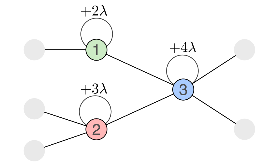
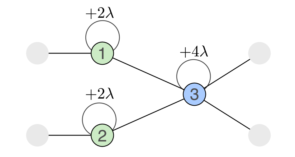
Figure 13: A schematic illustration of two graphs with self-loops weighted by the (loop-excluded) degree $d$ of each vertex, scaled by $\lambda$. The weights are displayed above each self-loop, and the label inside each vertex represents the corresponding $i$-th basis. For clarity, the vertices are colored according to their respective degree, while gray vertices hold no particular importance. (a) Assigning the state $(1,-1,0)^{T}$ to the three vertices leads to cancellation between the green (black•) and pink (black•) vertices at the blue (black•) vertex. However, due to the non-uniform self-loop weights, this state does not generally become an eigenstate. (b) The same state can still be an eigenstate via OBDHS.

In this section, we explore QMBS in both QLM and QDM, with a particular focus on how destructive interference is formed within the graph. The presence of non-uniformly weighted self-loops in these models, however, complicates the occurrence of such interference. Nevertheless, as noted, the self-loops at each vertex are assigned weights proportional to the number of flippable plaquettes $N_{\text{fp}}$, scaled by $\lambda$. This self-loop assignment allows certain interference zeros to persist around a subgraph, maintaining the state as an eigenstate—demonstrating the order-by-disorder phenomenon in the Hilbert space, as discussed in Sec. IV.4. By design, any shared eigenpair between this subgraph and the entire graph is independent of $\lambda$ for any non-zero $\lambda$, violating ETH. However, if $\lambda$ is zero, cancellation may involve other vertices with differing degrees, as shown in Fig. 13, ultimately altering the subgraph and the QMBS it hosts.

Subsequently, we will focus on Type-I and Type-IIIA scars, which are considered simpler because they are simultaneous eigenstates of both $\widehat{O}_{\text{kin}}$ and $\widehat{O}_{\text{pot}}$, and examples of OBDHS. As a result, the subgraphs hosting these QMBS have uniform vertex degrees and self-loops, surrounded by vertices with distinct degrees at their outer boundaries, as illustrated in Fig. 13. For Type-I scars, their localization is primarily driven by the bipartite structure of the graph, where vertices are confined to one of the bipartite subsets and share the same degree. In Sec. VI.3, we will utilize the coloring method discussed in Sec. III.3.2 as a search protocol for Type-I scars, leveraging the properties of bipartiteness and uniform vertex degrees. Meanwhile, Type-IIIA scars reside on subgraphs with connected vertices, reflected by their non-zero $\expectationvalue{\widehat{O}_{\text{kin}}}$, while still sharing the same vertex degree. Their localizability is ensured by OBDHS and Lemma III.2, where the vertices at the outer boundary of the subgraph belong to the same automorphism orbit. We will explore these in more detail in Sec. VI.4. Similarly, the coloring method will be employed for the search of Type-IIIA scars, although in this case, vertex degree is the only guiding property. Additionally, we will discuss the fictitious-particle description of these two types of QMBS in the respective sections.

On the other hand, our understanding of Type-II, IIIB, and IIIC scars is still incomplete, and we plan to address these QMBS in future work.

(a)

(b)

(c)

Figure 14: Illustration of different coloring schemes on the graph induced by QDM with lattice size $(4,4)$ in the flux sector $(W_{x},W_{y})=(0,0)$, with self-loops omitted for clarity. The force-directed algorithm is employed for graph layout. (a) Vertices are colored in black and white to indicate the bipartiteness. (b) Vertices are colored by their corresponding degree $d$. (c) Vertices are colored according to their automorphism orbits. The dashed cyan (black•) boxes highlight the vertices corresponding to 9 Type-I scars characterized by $(O_{\text{kin}},O_{\text{pot}})=(0,4)$. In particular, 8 of them are formed by the purple (black•) orbit. Additionally, the coral (black•) vertices, corresponding to the tuple $(\text{white},d=6)$, form another Type-I scar characterized by $(O_{\text{kin}},O_{\text{pot}})=(0,6)$. The remaining subgraphs fail to achieve cancellation on their outer boundaries and, therefore, cannot form scars. The label $i$ on each vertex is retained for consistency, though it holds no particular significance in this figure.

VI.3 Type-I scars

We begin by illustrating how the properties of bipartiteness and uniform vertex degrees can guide us to identify subgraphs hosting Type-I scars using the coloring method discussed in Sec. III.3.2. This approach centers on finding the Cartesian product of (i) bipartite subsets and (ii) vertex sets partitioned by their degrees. Vertices that satisfy both criteria form a potential subgraph that may host QMBS, with a subsequent cancelability test required at the outer boundary. Since the vertices in these subgraphs belong to either side of the bipartite subsets and consist of isolated vertices, Type-I scars are fully determined by the null space of the matrix $K$, which represents the hopping of these vertices to the outer boundary.

Specifically, as shown in Fig. 14a and Fig. 14b, we use two different coloring schemes to illustrate the graph induced by $\widehat{O}_{\text{kin}}$. In Fig. 14a, vertices are colored black and white to indicate their bipartiteness, while in Fig. 14b, vertices are colored according to their degree $d$. The potential $\widehat{O}_{\text{pot}}$ is ignored because it assigns weights on self-loops by degree, which is already effectively represented by the vertex colors. We denote the bipartite subsets as $V=V_{b}\cup V_{w}$, and the partition by vertex degree as $V=V_{d_{1}}\cup V_{d_{2}}\cup\cdots$, where $V_{d}=\{v\in V\text{ | }\text{deg}(v)=d\}$. The Cartesian product of these two vertex colorings assigns a tuple to each vertex $v_{i}\in V$, such as $(\text{black},d=4)$, as shown by the dashed cyan (black•) boxes in Fig. 14c. We then partition the vertices based on these tuples, creating subgraphs that require further examination for cancelability by computing the null space of the matrix $K$, often using the bipartite projection $G^{2}$, as discussed in Sec. III.3.3. In practice, the graph induced by $KK^{T}$ often consists of further disconnected components, allowing us to compute their null spaces separately and further reduce the computational complexity. Our numerical results are summarized in Table 3, with the details of the numerical implementation provided in [140].

Our numerical investigation suggests that Type-I scars can often be subdivided into further orbits, as depicted in Fig. 14c. Vertices encircled by the dashed cyan (black•) boxes contain 3 orbits, forming 9 Type-I scars characterized by $(O_{\text{kin}},O_{\text{pot}})=(0,4)$ (for clarity, the notation $\expectationvalue{\cdot}$ for expectation value is omitted). Among these, the purple (black•) orbit contains 8 scars, which can be further distinguished by examining the translation and charge conjugation symmetries of the basis. We will explore these in more detail in Sec. VI.3.1. The remaining scar is formed by all 3 orbits within the dashed cyan (black•) boxes, making it sub-extensive on the graph. Additionally, the coral (black•) vertices form another Type-I scar characterized by $(O_{\text{kin}},O_{\text{pot}})=(0,6)$.

We have also found that while our coloring method is sufficient for identifying Type-I scars, it is not always optimal, as expected. Numerical studies reveal that some orbits do not contribute to Type-I scars, as shown in Table 3. These orbits contribute no weight to the scar eigenstates, appearing as trivial interference zeros, and can, therefore, be excluded from the subgraph constructed by the coloring method. Although the coloring method works efficiently for QDM, it tends to capture more irrelevant orbits in QLM. Currently, we lack the necessary insights to incorporate the properties of these irrelevant orbits and develop a better coloring scheme. Further research is needed to address this in the future.

VI.3.1 Fictitious-particle description

Figure 15: A selection of representative basis states is shown from the graph induced by QDM on a lattice of size $(4,4)$ in the flux sector $(W_{x},W_{y})=(0,0)$. The 16 chosen vertices labeled by $i$ are arranged in a $4\times 4$ grid, with each associated basis state displayed beneath its corresponding vertex. The vertices are colored to match those in the graph, with the colors serving only to distinguish the vertices from one another. Here, we use the labeling scheme outlined in Appendix A for the vertex label $i$.

In this section, we examine the orbits contributing to Type-I scars and provide a fictitious-particle description for these vertices as the basis. Notably, previous investigations of QLM and QDM have focused on the fictitious-particles in these QMBS, which manifest as singlet-like or more complicated entanglement structures [94, 57]. These QMBS exhibit area-law entanglement entropy, as the lattice can always be bipartitioned in a way that avoids cutting through them.

For simplicity, we will focus on the singlet-like fictitious-particles for demonstration. This is because its cancellation involves fewer vertices at the outer boundary. More complex entanglement structures typically require the involvement of more vertices, making them difficult to track analytically. As an example, we will consider the purple (black•) orbit discussed earlier in Fig. 14c, with the corresponding basis states shown in Fig. 15.

We begin by illustrating how graph automorphisms relate vertices within this orbit at the basis level. The vertices in this orbit can be grouped into 8 categories based on conventional global symmetries of the lattice, although they play equivalent roles under graph automorphisms. In Fig. 15, each row corresponds to one of these groups (with only 4 shown), with different colors used to represent them. Now, let us focus on the relationships between basis states organized in a column-wise direction:

• The blue (black•, 1st row) and orange (black•, 2nd row) basis states are related by performing the translation $T_{x\to x+2}$.

• The blue (black•, 1st row) and turquoise (black•, 3rd row) basis states are related by first performing the translation $T_{x\to x+1}$, followed by the charge conjugation, which reverses the direction of every link. Alternatively, these basis states can be associated by a $180^{\circ}$ rotation about the axis at $(2,2)$, directed outward from the page. This rotation is also equivalent to reflecting the lattice across the horizontal and vertical axes at $x=2$ and $y=2$, which divide the lattice into two equal halves.

• The blue (black•, 1st row) and claret (black•, 4th row) basis states are related by an $-90^{\circ}$ rotation about the axis at $(2,2)$, directed outward from the page.

On the other hand, when examining the row-wise direction, no clear global symmetry can relate these basis states. Instead, these basis states are associated by sublattice symmetry. For instance, the blue (black•) vertices, labeled by 5 and 15, are identical except for the third column of plaquettes, situated between the vertical lines $x=2$ and $x=3$. These two states are related by sublattice symmetry, where a translation $T_{y\to y+2}$ is applied to this sublattice. This transformation is somewhat analogous to rotating a single face of a Rubik’s Cube. A similar observation applies to every basis state in the row-wise direction. Thus, we conclude that the automorphism orbit can be divided into two components: one governed by conventional global lattice symmetries and the other by sublattice symmetry. However, the latter one is dependent on the lattice size.

To illustrate the cancellation pattern, we begin by representing each basis state with its corresponding vertex label $i$, denoted as $\ket{i}$, as expressing the full 2D spin configuration can be cumbersome. Readers are encouraged to verify that the basis states shown in Fig. 15 belong to the same bipartite subset by examining the links involved in the product for the parity operator $\widehat{C}_{\mu}$. Additionally, each plaquette is marked by the coordinates of its lower-left site r, denoted as $\Box_{(x,y)}$.

Consider the first two basis states highlighted in blue (black•) in Fig. 15, $\ket{5}$ and $\ket{15}$. We observe the following cancellations:

$$U_{\Box_{(2,0)}}\ket{5}-U_{\Box_{(2,2)}}\ket{15} =0\text{,}$$ (32)

$$U_{\Box_{(2,2)}}^{\dagger}\ket{5}-U_{\Box_{(2,0)}}^{\dagger}\ket{15} =0\text{,}$$

while noting that the plaquettes $\Box_{(2,1)}$ or $\Box_{(2,3)}$ can also be affected, as they each contain one vulnerable link. A similar cancellation pattern occurs for any pair of basis states, where one is colored in darker blue and the other in lighter blue. The complete cancellation pattern for this QMBS is summarized as a graph in the inset of Fig. 14c. In particular, the plaquettes $\Box_{(2,0)}$ and $\Box_{(2,2)}$ form singlet-like fictitious-particles, which is "concatenated" with another singlet formed by $\Box_{(0,1)}$ and $\Box_{(0,3)}$. These QMBS are referred to as lego scars in [94], highlighting the combinatorial nature of these fictitious-particles, although their combination is constrained by the gauge conditions of the system.

VI.3.2 Topological ICQMBS

In Fig. 15, we show explicitly how the ICQMBS can be represented using the corresponding basis. Now, we can explicitly discuss the robustness of these states protected by the local topology of the Fock space graph. Take the ICQMBS represented in the inset, $|\psi_{tICQMBS}\rangle=\frac{1}{2}\left(-|5\rangle+|15\rangle-|77\rangle+|74\rangle\right)$. The eigenvalue equation would be $\widehat{H}_{QDM}|\psi_{tICQMBS}\rangle=4\lambda|\psi_{tICQMBS}\rangle$. The Hamiltonian and eigenvector can be expressed in matrix form as

$$\widehat{H}_{QDM} =\left(\begin{array}[]{c|c|cc|c|cc|c|cc|c|cc|c}\ddots&\mathbf{0}_{c}&\vdots&\vdots&\mathbf{0}_{c}&\vdots&\vdots&\mathbf{0}_{c}&\vdots&\vdots&\mathbf{0}_{c}&\vdots&\vdots&\vdots\\ \hline\cr\mathbf{0}_{r,\langle 5|}&4\lambda&-1&-1&0&0&0&0&0&0&0&-1&-1&\cdots\\ \hline\cr\cdots_{\langle 4|}&-1&c_{4}\lambda&0&-1&0&0&0&0&0&0&0&0&\cdots\\ \cdots_{\langle 16|}&-1&0&c_{16}\lambda&-1&0&0&0&0&0&0&0&0&\cdots\\ \hline\cr\mathbf{0}_{r,\langle 15|}&0&-1&-1&4\lambda&-1&-1&0&0&0&0&0&0&\cdots\\ \hline\cr\cdots_{\langle 17|}&0&0&0&-1&c_{17}\lambda&0&-1&0&0&0&0&0&\cdots\\ \cdots_{\langle 75|}&0&0&0&-1&0&c_{75}\lambda&-1&0&0&0&0&0&\cdots\\ \hline\cr\mathbf{0}_{r,\langle 77|}&0&0&0&0&-1&-1&4\lambda&-1&-1&0&0&0&\cdots\\ \hline\cr\cdots_{\langle 73|}&0&0&0&0&0&0&-1&c_{73}\lambda&0&-1&0&0&\cdots\\ \cdots_{\langle 78|}&0&0&0&0&0&0&-1&0&c_{78}\lambda&-1&0&0&\cdots\\ \hline\cr\mathbf{0}_{r,\langle 74|}&0&0&0&0&0&0&0&-1&-1&4\lambda&-1&-1&\cdots\\ \hline\cr\cdots_{\langle 9|}&-1&0&0&0&0&0&0&0&0&-1&c_{9}\lambda&0&\cdots\\ \cdots_{\langle 71|}&-1&0&0&0&0&0&0&0&0&-1&0&c_{71}\lambda&\cdots\\ \hline\cr\vdots&\vdots&\vdots&\vdots&\vdots&\vdots&\vdots&\vdots&\vdots&\vdots&\vdots&\vdots&\vdots&\vdots\end{array}\right)$$ (33)

$$|\psi_{tICQMBS}\rangle =\frac{1}{2}\left(\begin{array}[]{cccccccccccccc}\mathbf{0}_{c}&-1&0&0&1&0&0&-1&0&0&1&0&0&\mathbf{0}_{c}\end{array}\right)^{T}\text{.}$$

Here, we use $\mathbf{0}_{r}$ and $\mathbf{0}_{c}$ to represent zero row vectors and zero column vectors with suitable length. $c_{t}$ corresponds to the unimportant coefficients for the potential energy of the state $t$. We explicitly show the relevant sub-matrix elements for the local topology of the Fock space graph. One can explicitly check the eigenvalue equation with simple matrix multiplication.

The robustness of the eigenvector is obvious since any real space local perturbation that modifies the elements outside the sub-matrix, i.e., the elements represented by $\cdots$, will not alter the eigenvalue equation and keep the $|\psi_{tICQMBS}\rangle$ as a non-thermal eigenstate. As expected, $|\psi_{tICQMBS}\rangle$ remains an eigenvector even when the perturbation breaks all the symmetries. i.e., translation symmetry, time-reversal symmetry, or even the Hermicity of the Hamiltonian. For example, we can consider changing the potential energy scale on $U_{\Box_{(2,1)}}$ from $\lambda$ to $\lambda_{(2,1)}\neq\lambda$. We can also modify the kinetic energy term on the same plaquette and turn it into $(t^{R}_{(2,1)}+it^{I}_{(2,1)})U_{\Box_{(2,1)}}+(t^{R}_{(2,1)}-it^{I}_{(2,1)})U_{\Box_{(2,1)}}^{\dagger}$ to break translation and time reversal symmetry simultaneously. Both operations will keep $|\psi_{tICQMBS}\rangle$ as an ICQMBS protected by the local topology of the Fock space graph. The robustness due to the local topology of the Fock space graph also suggests any required algebraic structure can be violated away from the interference pattern. Therefore, the tICQMBS of this kind goes beyond the projector embedding approach and the stable quasi-particle approach.

VI.4 Type-IIIA scars

Figure 16: The graph representation of QLM with lattice size $(4,4)$ in the flux sector $(W_{x},W_{y})=(0,0)$, where the vertices are colored black and white based on bipartiteness. The inset shows one of the two identical subgraphs with $d=8$, with vertices colored according to their orbits. These two subgraphs remain bipartite, with the purple (black•) orbit corresponding to the white subset and the rest to the black subset in the main figure. The shaded dashed boxes denote the orbits that do not contribute to the Type-IIIA scar, effectively splitting the sphere-like subgraph into two hemispheres. Consequently, only the purple (black•) and pale-green (black•) orbits contribute to Type-IIIA scars. The force-directed layout is used for both the main figure and the inset. The label $i$ on each vertex is retained for consistency, though it holds no particular significance in this figure.

Similarly, we start by demonstrating how the coloring method can help identify subgraphs that host Type-IIIA scars, followed by a fictitious-particle description of these QMBS in Sec. VI.4.1. In this case, however, the search is less efficient, as the only guiding property is the vertex degree. Type-IIIA scars are closely related to Type-I scars but differ in having non-zero integer kinetic energy, indicating that the subgraphs hosting these QMBS consist of connected vertices, rather than being localized within one of the bipartite subsets.

As shown in Fig. 16, vertices with degree $d=8$ are highlighted by dashed cyan (black•) boxes, forming stacked black and white layers that create two individually connected yet still bipartite subgraphs. These subgraphs are sandwiched between two additional black layers at their outer boundaries, allowing for potential cancellation at the outer boundaries as described by Lemma III.2. Notably, only the $\pm 2$-eigenvectors of these subgraphs can be localized. Similar to Type-I scars, the coloring method tends to capture more orbits than necessary; in this case, only the purple (black•) and pale-green (black•) vertices contribute to Type-IIIA scars, as depicted in the inset of Fig. 16. The relevant orbits exhibit an $A$-$B$ sublattice structure, as reported in [57], which we will explore further in Sec. VI.4.1. Interestingly, the orbits associated with the $\pm 2$-eigenvectors are identified as cycle graphs for certain lattice sizes, as detailed in Appendix D. As a side note, we state that any bipartite graph cannot contain cycles of odd length, and the simplest bipartite graph showing $\pm 2$ eigenvalues is the cycle graph $C_{4}$.

To find these scars, we start by partitioning the vertices by degree, $V=V_{d_{1}}\cup V_{d_{2}}\cup\cdots$, where $V_{d}=\{v\in V\text{ | }\text{deg}(v)=d\}$, and denote the induced subgraph as $G_{d}=G[V_{d}]$ with its associated adjacency matrix $M$. In general, we can solve the full eigenvalue problem $M\textbf{x}=\mu\textbf{x}$, not limited to the $\pm 2$-eigenvectors. If $G_{d}$ consists of further disconnected components, we can also solve the eigenvalue problems for each component separately. Once solved, we test the cancelability of every x on the outer boundary by verifying $K^{T}\textbf{x}=0$. Although this still requires a full (or at least partial) ED on the subgraph, the size of these subgraphs is considerably smaller than the whole graph, as shown in Table 3, allowing us to achieve relatively large lattice sizes.

In the presence of degeneracies, the cancelability test becomes more subtle, as certain degenerate eigenstates may resist cancellation at the outer boundary. Without loss of generality, let us denote the two sets of eigenvectors as $\textbf{x}_{i}$ and $\textbf{y}_{i}$, where $\{\textbf{x}_{i}\text{ | }K^{T}\textbf{x}_{i}=0\}$ and $\{\textbf{y}_{i}\text{ | }K^{T}\textbf{y}_{i}\neq 0\}$ are both degenerate $\mu$-eigenvectors of $M$, but $\textbf{y}_{i}$ are not localizable. The cancelability test typically applies to the linear superpositions of $\textbf{x}_{i}$ and $\textbf{y}_{i}$, leading to

$$K^{T}\left(\sum_{i}\alpha_{i}\textbf{x}_{i}+\sum_{j}\beta_{j}\textbf{y}_{j}\right)\neq 0\text{,}$$ (34)

which is generally non-zero. To separate the $\textbf{y}_{i}$ contributions, we need to find the specific choice of $\beta$ coefficients such that the above Eq. 34 vanishes, that is,

$$K^{T}\begin{pmatrix}\textbf{x}_{1}&\cdots&\textbf{y}_{1}&\cdots\end{pmatrix}\begin{pmatrix}\alpha_{1}\\ \vdots\\ \beta_{1}\\ \vdots\end{pmatrix}=K^{T}U_{\mu}\Theta=0\text{.}$$ (35)

Consequently, this is equivalent to finding the null space of the matrix $K^{T}U_{\mu}$, and the scar eigenvectors are given by $U_{\mu}\Theta$, where $\Theta$ is a coefficient matrix of $\alpha_{i}$ and $\beta_{i}$.

While numerical results suggest only $\pm 2$-eigenvectors can achieve the cancellation on the outer boundary, we do not fully understand the uniqueness of the $\pm 2$ eigenvalues compared to other eigenvalues. We will discuss our preliminary understanding in Appendix D.

VI.4.1 Fictitious-particle description

Figure 17: A selection of representative basis states with vertex degree $d=8$ is depicted for QLM on a lattice of size $(4,4)$ in the flux sector $(W_{x},W_{y})=(0,0)$. All basis states have flippable plaquettes positioned on either the $A$ or $B$ sublattice. Notably, the first three columns on the left feature an equal number of clockwise and counterclockwise flippables. In contrast, the purple (black•) orbits in the last two columns have an unequal number of clockwise and counterclockwise flippables, differing by two. Specifically, the state $\ket{182}$ is selected from one of the cyan (black•) boxes in Fig. 16, while the other basis states in pale-green (black•) and purple (black•) are from the other cyan (black•) box. The additional plaquette variable in the basis, represented by a diagonally split black-and-white square, indicates two vulnerable links at the corners.

Figure 18: Two additional representative basis states with vertex degree $d=8$ are shown for QLM on a lattice of size $(4,4)$ in the flux sector $(W_{x},W_{y})=(0,0)$. These orbits do not contribute to Type-I or Type-IIIA scars, as they either lack the $A$-$B$ sublattice structure or feature an unequal number of clockwise and counterclockwise flippable plaquettes, differing by more than two.

We begin by examining all basis states with vertex degree $d=8$, as depicted in both Fig. 17 and 18. These orbits clearly display an $A$-$B$ sublattice structure, where flippable plaquettes are positioned on one sublattice, arranged either diagonally or off-diagonally. The only exception is the orbit in sky-blue (black•) in Fig. 18. Consequently, for basis states with an $A$-$B$ sublattice structure, the number of flippable plaquettes, $N_{\text{fp}}$, is always half of the system size, i.e., $N_{\text{fp}}=L_{x}L_{y}/2$. Notably, the $A$-$B$ sublattice structure arises because neighboring plaquette operators $U_{\Box}$ do not commute, and the division of $A$ and $B$ sublattices results in two sets of mutually commuting plaquettes.

It is worth noting that the basis states shown in Fig. 17 are also responsible for Type-I scars. One type of Type-I scar is formed by the first three orbits (in skin black•, yellow black•, and pale-green black•), characterized by an equal number of clockwise and counterclockwise flippable plaquettes, denoted as $n_{\text{cw}}$ and $n_{\text{ccw}}$, respectively. The other two types of Type-I scars are formed by the individual purple (black•) orbits, which differ based on whether the flippable plaquettes appear in the $A$ sublattice or $B$ sublattice. Both types are characterized by $|n_{\text{cw}}-n_{\text{ccw}}|=2$, which could correspond to either 5 clockwise and 3 counterclockwise flippable plaquettes, or vice versa. Similarly, these Type-I scars also exhibit singlet-like or more complex fictitious-particle structures, with the fictitious-particles positioned along either diagonal or off-diagonal directions on the sublattice. For more details, interested readers may refer to [57], where these scars are referred to as sublattice scars. Finally, the number of such Type-I scars is summarized in Table 3.

On the other hand, Type-IIIA scars consist solely of the pale-green (black•) and purple (black•) orbits, as shown in Fig. 17. These orbits belong to different bipartite subsets, as previously depicted in Fig. 16. Readers can verify this by examining the action of the parity operator $\widehat{C}_{\mu}$ on these basis states. We observe the following cancellations occurring for the basis states in the purple (black•) orbit:

$$U_{\Box_{(2,1)}}^{\dagger}\ket{29}-U_{\Box_{(0,1)}}^{\dagger}\ket{34}=0\text{,}$$ (36)

$$U_{\Box_{(0,3)}}^{\dagger}\ket{29}-U_{\Box_{(0,1)}}^{\dagger}\ket{518}=0\text{,}$$

where the plaquette flips are applied to flippable plaquettes adjacent to non-flippable plaquettes containing a vulnerable link, which, when affected, changes $N_{\text{fp}}$ from 8 to 10. Notably, all basis states in the purple (black•) orbit consistently contain $N_{\text{fp}}/2$ such non-flippable plaquettes and are solely related by lattice translation or charge conjugation.

The cancellations in Eq. 36 resemble the destructive interference found in Type-I scars, effectively annihilating these vertices on the opposite bipartite subset. As shown in Table 3, this is reflected in the number of degenerate Type-I scars in the $|n_{\text{cw}}-n_{\text{ccw}}|=2$ sector, which matches that of Type-IIIA scars. These cancellations require the scar eigenvectors to have equal amplitudes on the involved vertices, differing only in their signs, strongly suggesting that the scar eigenvectors should have integer eigenvalues. Additionally, we observe the plaquette flip on the following basis states in the pale-green (black•) orbit:

$$U_{\Box_{(1,2)}}^{\dagger}\ket{30}=U_{\Box_{(3,0)}}^{\dagger}\ket{302}$$ (37)

$$=U_{\Box_{(3,2)}}^{\dagger}\ket{31}=U_{\Box_{(1,0)}}^{\dagger}\ket{100}=\ket{29}\text{,}$$

indicating that these four basis states are connected to the state $\ket{29}$ in the purple (black•) orbit.

Without loss of generality, we can focus on the five basis states involved in Eq. 37, leading to the following expression for Type-IIIA scars:

$$\ket{\psi}_{\pm 2}= \;\alpha\left(\ket{30}+\ket{302}\right)+\beta\left(\ket{31}+\ket{100}\right)$$ (38)

$$\pm(\alpha+\beta)\ket{29}+\text{other terms}\text{,}$$

where $\alpha$ and $\beta$ are eigenvector coefficients constrained by Eq. 36 and subject to normalization. As a result, the local plaquette flips in Eq. 37 naturally lead to:

$$\left(U_{\Box_{(1,2)}}^{\dagger}+U_{\Box_{(3,0)}}^{\dagger}+U_{\Box_{(3,2)}}^{\dagger}+U_{\Box_{(1,0)}}^{\dagger}\right)\ket{\psi}_{\pm 2}$$ (39)

$$=2(\alpha+\beta)\ket{29}+\text{other terms}\text{.}$$

At this stage, the presence of eigenvalue $\pm 2$ has become evident by comparing Eq. 38 and Eq. 39, as well as by analyzing their finite overlap at $\ket{29}$. The remaining terms can be derived from the states within these two orbits, demonstrating the same cancellation process. In particular, we highlight the pairwise cancellations occurring along the "equator" of the sphere-like graph, as shown in Fig. 16. This cancellation is also explained by Eq. 37, where the four pale-green (black•) vertices can cancel out at the purple (black•) vertex. Finally, the complete cancellation pattern is summarized as a graph in Fig. 21 in the appendix.

In summary, Type-IIIA scars can only occur in QLM with an $A$-$B$ sublattice structure, a configuration that is prohibited by the gauge constraints in QDM. It would be valuable to explore the graph-theoretical significance of the $A$-$B$ sublattice structure and the property of $|n_{\text{cw}}-n_{\text{ccw}}|$. A deeper understanding of these features could lead to an improved coloring method that exploits these characteristics for a more efficient search for scars. Currently, we do not have a comprehensive understanding of the implications of these properties or the uniqueness of the $\pm 2$ eigenvalues. Notably, the eigenvectors corresponding to the $\pm 2$ eigenvalues consistently represent the highest and lowest eigenstates on the subgraphs hosting Type-IIIA scars. Some of our preliminary insights will be discussed in Appendix D.

QLM
$(L_{x},L_{y})$	Graph size	Type	Subgraph size	Number of orbits	Degeneracy	$(O_{\text{kin}},O_{\text{pot}})$
$(4,2)$	38	I I	16 $\{6^{2}\}$	1 $\{1^{2}\}$	4 $\{2^{2}\}$	$(0,5)$ $(0,4)$
$(6,2)$	282	I I	$\{14^{2}\}$ $\{24^{2}\}$	$\{2^{2}\}$ $\{1^{2}\}$	$\{2^{2}\}$ $\{1^{2}\}$	$(0,6)$ $(0,5)$
$(4,4)$	990	I I IIIA	$\{48^{2},204\to 124\}$ $224\to 192$ $\{110^{2}\to 96^{2}\}$	$\{1^{2},5\to 3\}$ $2\to 1$ $\{4^{2}\to 2^{2}\}$	$\{3^{2},20\}$ 12 $\{3^{2}\}$	$(0,8)$ $(0,6)$ $(\pm 2,8)$
$(6,4)$	32,810	I I IIIA	$\{552^{2}\to 192^{2},2988\to 1020\}$ $3792\to 1536$ $\{1160^{2}\to 384^{2}\}$	$\{8^{2}\to 2^{2},37\to 16\}$ $26\to 8$ $\{27^{2}\to 5^{2}\}$	$\{1^{2},44\}$ 8 $\{1^{2}\}$	$(0,12)$ $(0,10)$ $(\pm 2,12)$
QDM
$(L_{x},L_{y})$	Graph size	Type	Subgraph size	Number of orbits	Degeneracy	$(O_{\text{kin}},O_{\text{pot}})$
$(4,2)$	16	I I	4 8	2 1	1 3	$(0,4)$ $(0,3)$
$(6,2)$	76	I	$\{6^{2},18\}$	$\{1^{2},2\}$	$\{1^{2},1\}$	$(0,4)$
$(4,4)$	132	I I	32 48	1 3	1 9	$(0,6)$ $(0,4)$
$(6,4)$	1,456	I	$\{5^{6}\to 4^{6}\}$	$\{3^{6}\to 2^{6}\}$	$\{1^{6}\}$	$(0,4)$
$(8,4)$	17,412	I I I	$1664\to 64$ $608\to 256$ $\{5^{8}\to 4^{8}\}$	$31\to 3$ $8\to 2$ $\{2^{8}\to 1^{8}\}$	4 16 $\{1^{8}\}$	$(0,8)$ $(0,7)$ $(0,4)$

Table 3: Summary of QMBS across various lattice dimensions $(L_{x},L_{y})$ for both QLM and QDM in the flux sector $(W_{x},W_{y})=(0,0)$, with the size of the corresponding Hilbert space (as a graph) shown in the second column. Here, curly brackets $\{\cdot\}$ denote a set of numbers, indicating that each subgraph may contain further disconnected components, each with corresponding orbits and degeneracies. The order of numbers within the set remains fixed within the same row. Superscripts in curly brackets $\{\cdot^{*}\}$ are a shorthand notation for repeated numbers. For instance, QDM on a lattice size $(6,4)$ has 6 Type-I scars, each corresponding to a subgraph of size 5, containing 3 orbits, and 1 possible cancellation on the graph (indicated by its degeneracy). The arrow $(\cdot)\to(*)$ indicates that further reductions of the subgraph size and orbits are possible after removing all trivial interference zeros. Here, the left-hand number $(\cdot)$ represents the actual number captured by the coloring schemes and considered in our numerical study, while the right-hand number $(*)$ denotes the number after removing the zero entries in the scar eigenvectors.

VI.5 Summary for the 1D spin-1 XY model and the 2D QLM/QDM

We have applied these graph theory insights to two lattice models: the 1D spin-1 XY model and the 2D $U(1)$ LGTs. The former is an unconstrained model, while the latter is a constrained system. The graph representations of both models are predominantly bipartite, ensured by the parity operator, with a few exceptions for the spin-1 XY model under PBC when $L$ is odd, as detailed in Appendix C. In bipartite graphs, destructive interference has a straightforward explanation: QMBS are localized in one of the bipartite subsets, with their amplitudes canceling out in the opposite subset. However, the presence of self-loops in the graph can complicate this cancellation, warranting further study.

In the 1D spin-1 XY model, self-loops are uniformly weighted within each $S^{z}$ sector and thus do not affect destructive interference. All QMBS can be easily understood based on the bipartite structure of the graph. In contrast, the 2D $U(1)$ LGTs exhibit non-uniformly weighted self-loops, making cancellation patterns more complex. Nonetheless, since the potential term assigns weights to self-loops based on vertex degrees, subgraphs with uniform vertex degrees can still produce cancellations at their outer boundaries, resembling some of the cancellation mechanisms seen in the underlying loopless graph. Building on these observations, we propose a vertex partitioning scheme that leverages the bipartite structure and vertex degrees, facilitating a programmatic search for these subgraphs, followed by tests to confirm the cancelability of their eigenstates at the outer boundaries. Although limited to Type-I and IIIA scars, this method enables the direct construction of scar eigenstates at a lower cost compared to a full ED study.

We have also investigated the quasi-particles in these QMBS at the basis level. In the spin-1 XY model, the two bipartite subsets naturally give rise to two types of previously identified QMBS [75], with fictitious-particles corresponding to bimagnons and bond-bimagnons. Additionally, we discovered that these fictitious-particles can appear in combinatorial patterns that have not been previously recognized. Depending on the boundary conditions, other quasi-particles, such as isolated magnons or paired magnons, can also emerge. In contrast, in the 2D $U(1)$ LGTs, Type-I and IIIA scars exhibit singlet-like or more complex entanglement structures, as previously identified through ED [94, 57]. Similarly, these fictitious-particles also emerge in a combinatorial fashion in larger lattice sizes, though constrained by gauge conditions. While these fictitious-particles are difficult to track analytically, we have demonstrated how they are annihilated by local operators. Our investigation into these basis states also reveals a sublattice symmetry in the lattice, a symmetry captured by automorphism orbits that depend on lattice sizes.

It is worth noting that our numerical studies provide several insights when compared to previous ED research on 2D $U(1)$ LGTs. In Table 3, we compare our results with those from ED studies [94, 57]. Notably, we identified missing Type-I scars in QDM with ladder geometries $(L_{x},2)$, which had not been observed previously. This absence in earlier studies is likely due to the challenge of distinguishing low-entanglement outliers in small lattice systems during the post-selection of QMBS. Additionally, we did not find any Type-I or IIIA scars for QDM on lattice sizes $(6,6)$ and $(8,6)$ in the flux sector $(W_{x},W_{y})=(0,0)$, with Hilbert space (or graph) sizes of $44,176$ and $1,504,896$, respectively. This finding is consistent with previous ED studies. For Type-IIIA scars, this can be attributed to the absence of an $A$-$B$ sublattice structure in QDM, as it is forbidden by the gauge constraint. For Type-I scars, we analyzed the subgraphs identified through the coloring method, particularly with the bipartite projection $G^{2}$, and found that the subgraph $G^{2}[V_{d}]$ often consists solely of isolated vertices. This suggests poor connectivity within $G^{2}[V_{d}]$, requiring paths that traverse vertices of other degrees. However, we do not yet fully understand how the gauge constraint prevents these edge connections. Moreover, the separation protocol for degenerate $\mu$-eigenvectors, discussed in Sec. VI.4, is applied to QLM on a $(6,4)$ lattice. However, for QLM on a $(4,4)$ lattice, all $\pm 2$-eigenvectors are localizable and do not require additional separation. This observation is expected, as different orbits can contribute to the same degenerate eigenvalues.

VII Conclusions

In this work, we demonstrated that a family of quantum many-body scars (QMBS) can be understood as strictly localized orbitals on the Fock space graph, confined by many-body destructive interference—an effect reminiscent of compact localization in flat-band physics. We termed these states interference-caged quantum many-body scars (ICQMBS). While the connection between flat-band physics and QMBS beyond one dimension has previously remained unexplored due to the complexity of interference patterns in Fock space, we show that this perspective offers powerful insights into nonthermal eigenstates.

Starting from the anomalous entanglement properties of QMBS, we generalized the notion of compact localization from single-particle flat-band systems to many-body Fock space graphs. To analyze interference structures, we developed a graph-theory-based search algorithm targeting pairwise destructive interference in models with translational symmetry, time-reversal symmetry, and bipartite Fock space representations. These symmetries allow for a systematic topological analysis of the Fock space graph.

Crucially, we identified interference zeros as the fundamental building blocks for understanding ICQMBS. This insight enabled a formal description that demonstrates the nonthermal nature of ICQMBS through vanishing expectation values of local observables—without relying on symmetry assumptions.

Our framework reveals two key advances. First, through a graph-theoretical lens, we conjecture that ICQMBS formation is governed by graph automorphisms and interference zeros distributed across distinct automorphism orbits. This link between graph automorphisms and weak ergodicity breaking has not been previously recognized. We tested this idea in the 1D spin-1 XY model—where QMBS are well understood—and extended it to two-dimensional quantum link and dimer models (QLM/QDM), uncovering novel interference patterns and clarifying the origin of the order-by-disorder phenomena in Hilbert space.

Second, drawing from the concept of local topology in flat-band systems, we proposed and verified the existence of topological ICQMBS (tICQMBS). These states exhibit robustness against all real-space local perturbations that preserve the local structure of the Fock space graph. We demonstrated this robustness in type-I scars of 2D QLM/QDM, where translation symmetry and time-reversal symmetry are broken, but the emergent tICQMBS persist due to protection by the local topology of the Fock space graph.

Our study raises several open questions that warrant further exploration:

• Although physical observables should, in principle, be basis-independent, we found that the computational basis uniquely reveals the destructive interference responsible for ICQMBS. It remains unclear whether similar interference mechanisms may emerge in other bases with low real-space bipartite entanglement, especially since the off-diagonal elements of the Hamiltonian typically become more complex in such cases, posing a challenge for algorithm development.

• In QLM and QDM, where analytical expressions for QMBS are elusive due to local constraints, a promising direction involves constructing tensor network representations—such as matrix product states (MPS) in 1D and projected entangled pair states (PEPS) in 2D. Inspired by prior work in the PXP model [132], these representations may enable the construction of exact scar states by imposing annihilation conditions from the local Hamiltonian.

• The system-size dependence of graph automorphisms complicates understanding their role in the thermodynamic limit. It remains an open problem to determine how the number of QMBS scales with system size. Previous work has proposed that Type-I scars grow exponentially [94] via zero modes or scar concatenation, but a graph-theoretic explanation for this behavior remains lacking.

• Our graph-theoretic approach provides an exact understanding of QMBS formation, but it opens broader questions about its applicability to real-time many-body dynamics, particularly beyond one dimension. While we focused on ETH-violating eigenstates, it is unclear how interference zeros influence dynamical ergodicity breaking [20, 21, 22, 141, 142]. The connection between graph theory and slow dynamics, as observed in constrained models like the quantum East model [101], suggests Fock space graph-based approach to study correlated dynamics is a promising future direction—particularly in light of recent advances in spectral graph theory [143].

• While our algorithm focuses on pairwise destructive interference, strictly localized states in flat-band systems suggest more complex cancellation patterns are possible. Developing a general method to identify ICQMBS beyond pairwise interference—especially in Fock space graphs without translation symmetry—remains an important open challenge.

• Finally, it remains to be seen how broadly our graph-based framework applies to other systems that host QMBS. A detailed comparison with other formalisms proposed in the literature [68, 69] may help to unify or distinguish different approaches to understanding scars and ergodicity breaking.

In summary, this work opens a new direction for studying QMBS as compactly localized states on the Fock space graph. By bridging concepts from graph theory, flat-band physics, and quantum many-body dynamics, we establish a framework that reveals new mechanisms for nonthermal eigenstate formation and stability for general spatial dimensions. Our results provide both conceptual and practical tools—such as an efficient search algorithm and the identification of topological protection—for future exploration of quantum many-body scars in a broad class of systems.

Appendix A The labeling scheme for each vertex in the graph

In this section, we discuss the assignment of vertex labels $i$ on the graph and their relationship to each spin configuration in both the 1D spin-1 XY model and the 2D $U(1)$ LGTs. It is important to note that, from the perspective of graph automorphisms, the choice of vertex label $i$ is somewhat arbitrary within the same orbit. However, we will explain the convention we have adopted here, which is consistent with that used in the main text.

A.1 Labeling scheme in the spin-1 XY model

Starting with the spin-1 XY model, the spin-1 configurations are naturally represented using the ternary numeral system. Specifically, we represent $\ket{+}$ as $2$, $\ket{0}$ as $1$, and $\ket{-}$ as $0$. For a spin configuration $\ket{s_{0}s_{1}\cdots s_{r}\cdots s_{L-1}}$ on a lattice of length $L$, the vertex label $i$ is determined by the corresponding decimal number:

$$i=3^{L}-1-\sum_{r=0}^{L-1}s_{r}\,3^{r}\text{,}$$ (40)

where a reversed order is chosen so that the fully polarized state $\ket{\Omega^{\prime}}=\bigotimes_{r=0}^{L-1}\ket{+}_{r}$ corresponds to the label $i=0$. For example, for a lattice of length 3, the labels are assigned as follows:

$$\ket{+++} \text{ is labeled by }i=0\text{,}$$

$$\ket{++\,0\,} \text{ is labeled by }i=1\text{,}$$

$$\ket{++-} \text{ is labeled by }i=2\text{,}$$

$$\qquad\vdots$$

$$\ket{---} \text{ is labeled by }i=26\text{.}$$

A.2 Labeling scheme in the 2D $U(1)$ LGTs

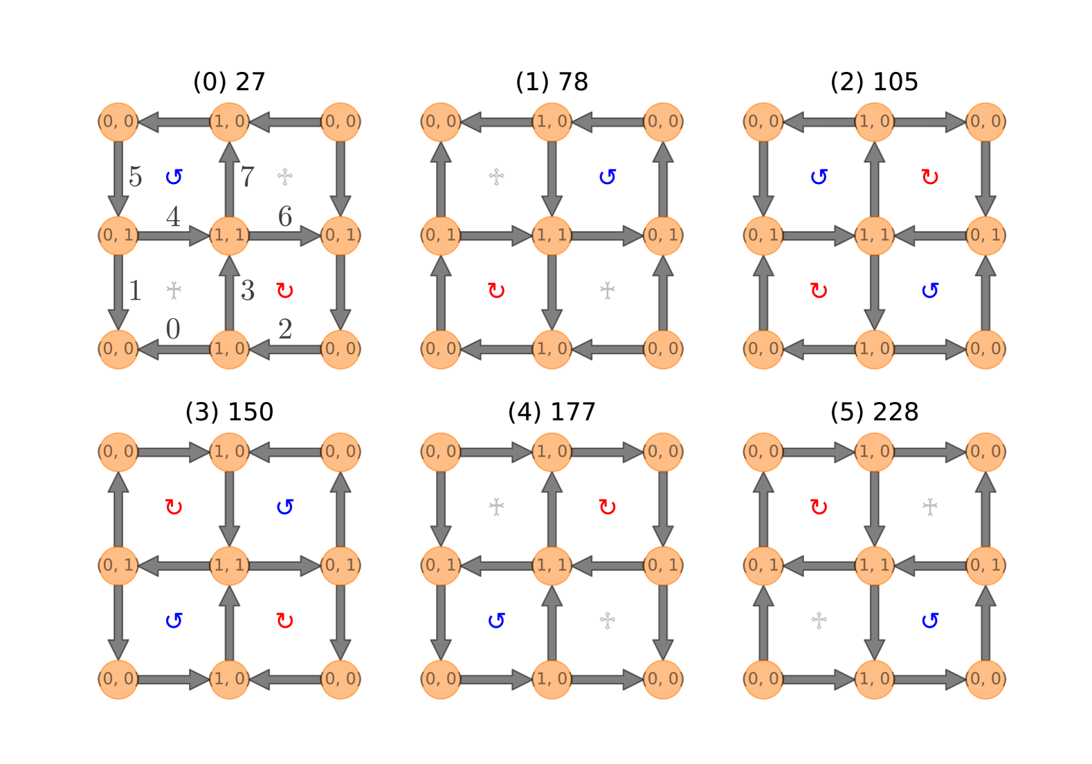
Figure 19: All six possible basis states for QLM of lattice size $(2,2)$ in the flux sector $(W_{x},W_{y})=(0,0)$. The two numbers "$(i)\,\bar{i}$" above each basis state represent the vertex label and the absolute label, respectively. The numbers next to each link in the basis state labeled "$(0)\,27$" (on upper-left) indicate the coordinate label $i_{c}$ for links. For clarity, the sites and links from the first column and row are repeated at the opposite boundary.

Next, we consider the 2D $U(1)$ LGTs, starting with the coordinate system used to label each link. For a link labeled by the tuple $(\textbf{r},\hat{\mu})$, where $\textbf{r}=(x,y)^{T}$ and $\hat{\mu}=\hat{x},\hat{y}$, its coordinate label $i_{c}$ (not to be confused with the vertex label $i$) is given by

$$i_{c}=2(x+L_{x}y)+\mu\text{,}$$ (41)

where $\mu=0$ for horizontal links and $\mu=1$ for vertical links (see also Fig. 19). It is natural to use the binary numeral system, specifically representing $\ket{\uparrow}$ as 1 and $\ket{\downarrow}$ as 0. Consequently, a spin configuration is represented by a binary sequence ordered by $i_{c}$ for each link, denoted as $\ket{s_{0}s_{1}\cdots s_{l}\cdots s_{N_{l}-1}}$, where $N_{l}=2L_{x}L_{y}$ links are present under PBC.

However, due to the constraints nature of the system, not all spin configurations will occur. We denote the absolute label $\bar{i}$ as the corresponding decimal number for a given spin configuration:

$$\bar{i}=2^{N_{l}}-1-\sum_{l=0}^{N_{l}-1}s_{l}\,2^{l}\text{,}$$ (42)

where a reversed order is chosen so that the fully polarized state $\ket{11\cdots 1}$ corresponds to the label $\bar{i}=0$. The vertex label $i$ is then defined as the relative order of $\bar{i}$, counted from zero. Consequently, unless the absolute index $\bar{i}$ is known, it is generally difficult to reconstruct the spin configuration based on the vertex label $i$. However, if all possible spin configurations, constrained by the gauge, are enumerated and stored in a table, the relationship between $\bar{i}$ and $i$ can still be constructed by referencing this lookup table.

As an example, consider a $2\times 2$ lattice with zero charges on every sites, i.e., a QLM, as depicted in Fig. 19. There are six such basis states, which can be enumerated as follows:

$$\ket{00,01,10,11}\text{,}$$

$$\ket{01,00,11,10}\text{,}$$

$$\ket{01,10,10,01}\text{,}$$

$$\ket{10,01,01,10}\text{,}$$

$$\ket{10,11,00,01}\text{,}$$

$$\ket{11,10,01,00}\text{.}$$

The commas in the ket states are included for clarity. Readers are encouraged to verify that the links in these basis states are ordered according to $i_{c}$, and that the labels $\bar{i}$ and $i$ are consistent with those in Fig. 19.

Appendix B Interference zeros and null space of $\widehat{O}_{\text{kin}}$

The generality of interference zeros poses significant challenges in devising a systematic protocol for identifying ICQMBS in generic systems. Nonetheless, in this section, we demonstrate that even without a practical protocol for locating interference zeros, standard linear algebra algorithms can be utilized for this purpose. Specifically, this involves analyzing the null space of $\widehat{O}_{\text{kin}}$, a task that standard linear algebra toolkits can efficiently handle. However, this method is restricted to QMBS analogous to Type-I scars, which have vanishing kinetic energy, $\expectationvalue{\widehat{O}_{\text{kin}}}=0$. For QMBS characterized by non-zero kinetic energy, an efficient detection method remains unavailable at present.

To illustrate this approach, we will focus on the topology of the Fock space graph by analyzing the adjacency matrix of $\widehat{O}_{\text{kin}}$, while temporarily disregarding the effects of $\widehat{O}_{\text{pot}}$. It is important to note that $\widehat{O}_{\text{pot}}$ can introduce nontrivial contributions, as we will discuss in Sec. IV.4. But for now, we limit our analysis to $\widehat{O}_{\text{kin}}$. Suppose $\widehat{O}_{\text{kin}}$ has a nullity greater than zero. In this case, there exist nontrivial energy eigenstates $\ket{\mathrm{E}}$ in the Fock space such that:

$$\widehat{O}_{\text{kin}}\ket{\mathrm{E}}=0\text{.}$$ (43)

Expressing this in the Fock space basis, we have:

$$\sum_{ij}A_{v_{i},v_{j}}\ket{v_{i}}\bra{v_{j}}\times\sum_{k}c_{k}\ket{v_{k}}$$ (44)

$$=\sum_{i}\left(\sum_{j}A_{v_{i},v_{j}}c_{j}\right)\ket{v_{i}}=0\text{,}$$

where $c_{k}$ are the weights of the state $\ket{\mathrm{E}}$ in the Fock space basis and $A_{v_{i},v_{j}}$ represents the elements of the adjacency matrix of $\widehat{O}_{\text{kin}}$. Specifically, $A_{v_{i},v_{i}}=0$ since self-loops are excluded from the analysis. Consequently, for every vertex $v_{i}$, we expect

$$\tilde{c_{i}}\coloneqq\sum_{v_{j}\in\partial v_{i}}A_{v_{i},v_{j}}c_{j}=0,\quad\forall i\text{,}$$ (45)

where $\tilde{c_{i}}$ represents the redistributed weights from neighboring vertices $v_{j}$ into vertex $v_{i}$ via $A$. Here, the summation is taken over $v_{j}\in\partial v_{i}$, as $A_{v_{i},v_{j}}=0$ for unconnected vertices.

In linear algebraic terms, this condition reflects a linear combination of the $j$-th columns of $A$. If two or more columns of $A$ are linearly dependent, there exist nonzero coefficients $c_{j}$ such that their linear combination vanishes. In our graph terminology, this corresponds to the non-trivial interference zero formed by $v_{j}\in\partial v_{i}$. Conversely, if the columns are linearly independent, the coefficients $c_{j}$ must be trivially zero, corresponding to the parts of the Fock space that do not participate in ICQMBS and thereby are trivial interference zeros.

Thus, this analysis suggests that we can find interference zeros by solving the null space of $\widehat{O}_{\text{kin}}$. However, it is important to note that while existing linear algebra algorithms are highly optimized, they do not account for the assumption that the interference-caged subgraph occupies only a small portion of the Fock space graph, surrounded by trivial interference zeros on the rest of the Fock space graph. Consequently, in such cases, relying on null-space analysis often results in significant computational inefficiency. Thus, a more tailored approach remains necessary.

Appendix C QMBS in the spin-1 XY model under PBC for odd $L$—An example of non-bipartite graph

Figure 20: Graph representation of the $S^{z}=-2$ sector for a lattice of size $L=5$ under PBC and $J_{3}=0$. This non-bipartite graph is colored by its automorphism orbits, with self-loops omitted for clarity. To maximize the utility of the graph, the spin configuration is indicated next to each vertex in the upper-left area, while the wavefunction amplitude of QMBS is depicted in the lower-right area, shaded with a gray background.

In this section, we explore the non-bipartite graphs that emerge in the 1D spin-1 XY model under PBC when $L$ is odd. As the simplest example, we consider the $S^{z}=-2$ sector for $L=5$ with $J_{3}=0$, as shown in Fig. 20. This sector can host one QMBS, as indicated in Table 1 in the main text, which can be expressed as

$$\ket{\mathcal{S}_{\text{nb}}}=\mathcal{N} \sum_{r=1}^{L}\Big{[}(S_{r}^{+})^{2}\left(S_{r+1}^{+}+S_{r+2}^{+}\right)$$ (46)

$$-\left(S_{r-1}^{+}+S_{r}^{+}\right)(S_{r+1}^{+})^{2}\Big{]}\ket{\Omega}\text{,}$$

where individual magnons and bimagnons are inserted into the vacuum background at four adjacent sites, and $\mathcal{N}$ is a normalization factor. The basis states involved in this QMBS comprise an equal number of non-magnon states, ensuring their resilience for $D\neq 0$ and thereby demonstrating OBDHS. Utilizing PBC, this expression can be further simplified to

$$\ket{\mathcal{S}_{\text{nb}}} =\mathcal{N}\;\sum_{r}(S_{r}^{+})^{2}$$ (47)

$$\times\left(S_{r+2}^{+}+S_{r+1}^{+}-S_{r-1}^{+}-S_{r+2}^{+}\right)\ket{\Omega}\text{.}$$

For other $S^{z}$ sectors across various lattice sizes that are non-bipartite, similar QMBS can be generalized in a combinatorial fashion. Although non-bipartite, this QMBS is localized on a subgraph, where two types of cancellations at its outer boundary can be recognized.

We begin by examining the cancellation at the silver (black•) vertices, such as the state $\ket{-000-}$ (on top of Fig. 20):

$$h_{2,3}^{\text{kin}}\ket{-,+-,0-}-h_{3,4}^{\text{kin}}\ket{-0,+-,-}$$ (48)

$$+ h_{2,3}^{\text{kin}}\ket{-,-+,0-}-h_{3,4}^{\text{kin}}\ket{-0,-+,-}=0\text{,}$$

where the site $r$ is indexed starting from 1, and commas are included in the ket states for clarity. As a result, these four basis states cancel each other out at the state $\ket{-000-}$.

Additionally, we observe a similar cancellation at the polo-blue (black•) vertices, such as the state $\ket{-00-0}$ (near the center of Fig. 20):

$$h_{2,3}^{\text{kin}}\left(\ket{-,+-,-0}-\ket{-,-+,-0}\right)=0\text{,}$$ (49)

leading to a cancellation at the state $\ket{-00-0}$, which primarily differs from $\ket{-000-}$ by the separation of the bond-bimagnon and magnon.

As a result, both types of cancellation annihilate the bimagnon, similar to the process in $\ket{\mathcal{S}_{n}}$, with an additional magnon contributing to the cancellation. The vertices involved in this QMBS form a connected subgraph, represented by a line graph consisting of the Carolina-blue (black•) and pink (black•) orbits, as illustrated in Fig. 20. Additionally, the pentagram-like geometry of the graph suggests that we can focus on one of its five "angles", each consisting of four vertices — two in Carolina-blue (black•) and two in pink (black•). The basis states of these vertices correspond to those excited from the vacuum, as described in Eq. 46, and the states in each "angle" are related by lattice translations. The complete cancellation pattern of this QMBS is summarized in Fig. 20.

Appendix D Cycles appeared in Type-IIIA scars

(a)

(b)

Figure 21: One of the two disconnected subgraphs in $G_{d=8}$ of QLM on a $(4,4)$ lattice in the flux sector $(W_{x},W_{y})=(0,0)$. (a) Vertices contributing to Type-IIIA scars are colored by their respective automorphism orbits, while the remaining vertices are shown in white. Vertex labels indicate the eigenstate amplitudes, rounded to three decimal places. (b) One of the hemispheres from (a) after removing all white vertices.

Figure 22: One of the two largest disconnected subgraphs in $G_{d=12}$ of QLM on a $(6,4)$ lattice in the flux sector $(W_{x},W_{y})=(0,0)$. Vertices contributing to Type-IIIA scars are colored by their respective automorphism orbits, while the remaining vertices are shown in white. Vertex labels indicate the eigenstate amplitudes, rounded to three decimal places.

Figure 23: A selection of representative basis states responsible for Type-IIIA scars in QLM on a $(6,4)$ lattice in the flux sector $(W_{x},W_{y})=(0,0)$. The colored vertex above each basis state represents the corresponding automorphism orbits, and the two numbers "$(i)\,\bar{i}$" denote the vertex label and the absolute label, respectively.

In this section, we highlight the cycle graphs that host Type-IIIA scars observed in QLM on a $(6,4)$ lattice. Although these cycle graphs are not present in the QLM on a $(4,4)$ lattice, as discussed in the main text, we have observed pairwise cancellations for both lattice sizes within the subgraph $G_{d}=G[V_{d}]$, where the vertices share the same degree $d=L_{x}L_{y}/2$, half the system size. To better illustrate the complex cancellation pattern, we use a different convention for vertex colors and labels. Specifically, we replace the colors of vertices involved in pairwise cancellations, as well as those in irrelevant orbits, with white. Vertices contributing to Type-IIIA scars are retained and colored according to their respective automorphism orbits. Additionally, the eigenvector weights are displayed on each corresponding vertex label, rounded to three decimal places for clarity.

We begin with the case of a $(4,4)$ lattice, as illustrated in 21. Comparing this with Fig. 16 in the main text, we observe pairwise cancellations along the "equator" of this sphere-like graph, dividing it into two hemispheres, one of which is shown in Fig. 21b. However, these pairwise cancellations occur on vertices belonging to both the pale-green (black•) and purple (black•) orbits and are not accounted for by Lemmas III.1 and III.2. We can replicate this pairwise cancellation using simple toy graph like circular ladder graph of order 6, $\text{CL}_{6}$. In $\text{CL}_{6}$, two $C_{4}$ subgraphs on the opposite faces can be assigned with opposite signs of eigenvector weights, causing them to cancel out in the middle.

For QLM on a $(6,4)$ lattice, the subgraph $G_{d=12}$ comprises multiple disconnected components, with the two largest subgraphs, each containing 1160 vertices, hosting Type-IIIA scars. Their disconnected nature reflects the $A$-$B$ sublattice structure. One of these subgraphs is illustrated in Fig. 22, where basis states appear only on either the $A$ or $B$ sublattice. Notably, the vertices associated with Type-IIIA scars are identified as 8 cycle graphs $C_{48}$ within this subgraph. The eigenvector weights are uniformly distributed across each $C_{48}$, with values either uniformly $\pm 1$ or altering between $\pm 1$, and a normalization factor of $1/\sqrt{8\times 48}\approx 0.051$. This arrangement ensures that these 8 cycle graphs $C_{48}$ cancel each other out in a pairwise manner within this subgraph, and naturally give rise to the $\pm 2$ eigenvalues. We also examine the basis states within these cycle graphs, as shown in Fig. 23. We begin by focusing on the relationships between basis states in the first row:

• From the sky-blue (black•) to the pale-green (black•) vertex:

  $U_{\Box_{(0,1)}}\ket{30247}=\ket{30304}$.

• From the pale-green (black•) to the orange (black•) vertex:

  $U_{\Box_{(2,3)}}\ket{30304}=\ket{31535}$.

• From the orange (black•) to the yellow (black•) vertex:

  $U_{\Box_{(1,0)}}^{\dagger}\ket{31535}=\ket{29360}$.

• From the yellow (black•) to the purple (black•) vertex:

  $U_{\Box_{(3,2)}}\ket{29360}=\ket{29361}$.

A similar pattern is observed in the second row. These plaquette flips act on plaquettes that are not adjacent to non-flippable plaquettes with a vulnerable link. As a result, the total number of flippable plaquettes remains 12, while the difference between clockwise and counterclockwise flippable plaquettes fluctuates between 0 and 2, i.e., $|n_{\text{cw}}-n_{\text{ccw}}|=0$ or $2$. Consequently, the cycle graph $C_{48}$ is composed of six repeating segments, each consisting of a chain of eight vertices, including five from each orbit, as shown in the row-wise direction of Fig. 23. These segments follow the sequence "-black•-black•-black•-black•-black•-black•-black•-black•-", repeating six times throughout the cycle and creating an oscillating pattern between the sky-blue (black•) and purple (black•) vertices.

On the other hand, the pairwise cancellations for these 8 cycle graphs are more complex, requiring the involvement of all 8 cycles. Some of these cancellations are illustrated in Fig. 23, where for the first two columns, we observe the following:

• The sky-blue (black•) vertices:

  $U_{\Box_{(5,2)}}\ket{30247}-U_{\Box_{(1,2)}}\ket{30249}=0$.

• The pale-green (black•) vertices:

  $U_{\Box_{(1,2)}}^{\dagger}\ket{30304}-U_{\Box_{(5,2)}}^{\dagger}\ket{30306}=0$.

However, the remaining three columns do not form the correct pairs for cancellation and require other cycle graphs. For clarity, we will not demonstrate this here.

References

- Neumann [1929] J. v. Neumann, Beweis des ergodensatzes und des h-theorems in der neuen mechanik, Zeitschrift für Physik 57, 30 (1929).
- von Neumann [2010] J. von Neumann, Proof of the ergodic theorem and the h-theorem in quantum mechanics: Translation of: Beweis des ergodensatzes und des h-theorems in der neuen mechanik, The European Physical Journal H 35, 201 (2010).
- Tasaki [1998] H. Tasaki, From quantum dynamics to the canonical distribution: General picture and a rigorous example, Phys. Rev. Lett. 80, 1373 (1998).
- Goldstein et al. [2010] S. Goldstein, J. L. Lebowitz, R. Tumulka, and N. Zanghì, Long-time behavior of macroscopic quantum systems: Commentary accompanying the english translation of john von neumann’s 1929 article on the quantum ergodic theorem, The European Physical Journal H 35, 173 (2010).
- Deutsch [1991] J. M. Deutsch, Quantum statistical mechanics in a closed system, Phys. Rev. A 43, 2046 (1991).
- Srednicki [1994] M. Srednicki, Chaos and quantum thermalization, Phys. Rev. E 50, 888 (1994).
- Rigol et al. [2008] M. Rigol, V. Dunjko, and M. Olshanii, Thermalization and its mechanism for generic isolated quantum systems, Nature 452, 854 (2008).
- D’Alessio et al. [2016] L. D’Alessio, Y. Kafri, A. Polkovnikov, and M. Rigol, From quantum chaos and eigenstate thermalization to statistical mechanics and thermodynamics, Advances in Physics 65, 239 (2016).
- Trotzky et al. [2012] S. Trotzky, Y.-A. Chen, A. Flesch, I. P. McCulloch, U. Schollwöck, J. Eisert, and I. Bloch, Probing the relaxation towards equilibrium in an isolated strongly correlated one-dimensional bose gas, Nature physics 8, 325 (2012).
- Kaufman et al. [2016] A. M. Kaufman, M. E. Tai, A. Lukin, M. Rispoli, R. Schittko, P. M. Preiss, and M. Greiner, Quantum thermalization through entanglement in an isolated many-body system, Science 353, 794 (2016).
- Tang et al. [2018] Y. Tang, W. Kao, K.-Y. Li, S. Seo, K. Mallayya, M. Rigol, S. Gopalakrishnan, and B. L. Lev, Thermalization near integrability in a dipolar quantum newton’s cradle, Phys. Rev. X 8, 021030 (2018).
- Nandkishore and Huse [2015] R. Nandkishore and D. A. Huse, Many-body localization and thermalization in quantum statistical mechanics, Annu. Rev. Condens. Matter Phys. 6, 15 (2015).
- Abanin et al. [2019] D. A. Abanin, E. Altman, I. Bloch, and M. Serbyn, Colloquium: Many-body localization, thermalization, and entanglement, Reviews of Modern Physics 91, 021001 (2019).
- Šuntajs et al. [2020] J. Šuntajs, J. Bonča, T. c. v. Prosen, and L. Vidmar, Ergodicity breaking transition in finite disordered spin chains, Phys. Rev. B 102, 064207 (2020).
- Abanin et al. [2021] D. Abanin, J. H. Bardarson, G. De Tomasi, S. Gopalakrishnan, V. Khemani, S. Parameswaran, F. Pollmann, A. Potter, M. Serbyn, and R. Vasseur, Distinguishing localization from chaos: Challenges in finite-size systems, Annals of Physics 427, 168415 (2021).
- Sierant et al. [2024] P. Sierant, M. Lewenstein, A. Scardicchio, L. Vidmar, and J. Zakrzewski, Many-body localization in the age of classical computing, Reports on Progress in Physics 10.1088/1361-6633/ad9756 (2024).
- Bernien et al. [2017] H. Bernien, S. Schwartz, A. Keesling, H. Levine, A. Omran, H. Pichler, S. Choi, A. S. Zibrov, M. Endres, M. Greiner, et al., Probing many-body dynamics on a 51-atom quantum simulator, Nature 551, 579 (2017).
- Turner et al. [2018a] C. J. Turner, A. A. Michailidis, D. A. Abanin, M. Serbyn, and Z. Papić, Weak ergodicity breaking from quantum many-body scars, Nature Physics 14, 745 (2018a).
- Turner et al. [2018b] C. J. Turner, A. A. Michailidis, D. A. Abanin, M. Serbyn, and Z. Papić, Quantum scarred eigenstates in a rydberg atom chain: Entanglement, breakdown of thermalization, and stability to perturbations, Phys. Rev. B 98, 155134 (2018b).
- Heller [1984] E. J. Heller, Bound-state eigenfunctions of classically chaotic hamiltonian systems: Scars of periodic orbits, Phys. Rev. Lett. 53, 1515 (1984).
- Berry [1989] M. V. Berry, Quantum scars of classical closed orbits in phase space, Proceedings of the Royal Society of London. A. Mathematical and Physical Sciences 423, 219 (1989).
- Kaplan [1999] L. Kaplan, Scars in quantum chaotic wavefunctions, Nonlinearity 12, R1 (1999).
- Pai et al. [2019] S. Pai, M. Pretko, and R. M. Nandkishore, Localization in fractonic random circuits, Phys. Rev. X 9, 021003 (2019).
- Khemani et al. [2020] V. Khemani, M. Hermele, and R. Nandkishore, Localization from hilbert space shattering: From theory to physical realizations, Phys. Rev. B 101, 174204 (2020).
- Sala et al. [2020] P. Sala, T. Rakovszky, R. Verresen, M. Knap, and F. Pollmann, Ergodicity breaking arising from hilbert space fragmentation in dipole-conserving hamiltonians, Phys. Rev. X 10, 011047 (2020).
- Moudgalya et al. [2022a] S. Moudgalya, A. Prem, R. Nandkishore, N. Regnault, and B. A. Bernevig, in Memorial Volume for Shoucheng Zhang (World Scientific, 2022) pp. 147–209.
- Serbyn et al. [2021] M. Serbyn, D. A. Abanin, and Z. Papić, Quantum Many-Body Scars and Weak Breaking of Ergodicity, Nature Physics 17, 675 (2021), arXiv:2011.09486 [cond-mat, physics:nlin, physics:quant-ph].
- Papić [2022] Z. Papić, in Entanglement in Spin Chains: From Theory to Quantum Technology Applications (Springer, 2022) pp. 341–395.
- Moudgalya et al. [2022b] S. Moudgalya, B. A. Bernevig, and N. Regnault, Quantum many-body scars and Hilbert space fragmentation: a review of exact results, Reports on Progress in Physics 85, 086501 (2022b), publisher: IOP Publishing.
- Chandran et al. [2023] A. Chandran, T. Iadecola, V. Khemani, and R. Moessner, Quantum Many-Body Scars: A Quasiparticle Perspective, Annual Review of Condensed Matter Physics 14, 443 (2023), arXiv:2206.11528 [cond-mat, physics:quant-ph].
- Desaules et al. [2022] J.-Y. Desaules, F. Pietracaprina, Z. Papić, J. Goold, and S. Pappalardi, Extensive multipartite entanglement from su(2) quantum many-body scars, Phys. Rev. Lett. 129, 020601 (2022).
- Dooley [2021] S. Dooley, Robust quantum sensing in strongly interacting systems with many-body scars, PRX Quantum 2, 020330 (2021).
- Dooley et al. [2023] S. Dooley, S. Pappalardi, and J. Goold, Entanglement enhanced metrology with quantum many-body scars, Phys. Rev. B 107, 035123 (2023).
- Fendley et al. [2004] P. Fendley, K. Sengupta, and S. Sachdev, Competing density-wave orders in a one-dimensional hard-boson model, Phys. Rev. B 69, 075106 (2004).
- Lesanovsky and Katsura [2012] I. Lesanovsky and H. Katsura, Interacting fibonacci anyons in a rydberg gas, Phys. Rev. A 86, 041601 (2012).
- Keesling et al. [2019] A. Keesling, A. Omran, H. Levine, H. Bernien, H. Pichler, S. Choi, R. Samajdar, S. Schwartz, P. Silvi, S. Sachdev, et al., Quantum kibble–zurek mechanism and critical dynamics on a programmable rydberg simulator, Nature 568, 207 (2019).
- De Léséleuc et al. [2019] S. De Léséleuc, V. Lienhard, P. Scholl, D. Barredo, S. Weber, N. Lang, H. P. Büchler, T. Lahaye, and A. Browaeys, Observation of a symmetry-protected topological phase of interacting bosons with rydberg atoms, Science 365, 775 (2019).
- Browaeys and Lahaye [2020] A. Browaeys and T. Lahaye, Many-body physics with individually controlled rydberg atoms, Nature Physics 16, 132 (2020).
- Ebadi et al. [2021] S. Ebadi, T. T. Wang, H. Levine, A. Keesling, G. Semeghini, A. Omran, D. Bluvstein, R. Samajdar, H. Pichler, W. W. Ho, et al., Quantum phases of matter on a 256-atom programmable quantum simulator, Nature 595, 227 (2021).
- Semeghini et al. [2021] G. Semeghini, H. Levine, A. Keesling, S. Ebadi, T. T. Wang, D. Bluvstein, R. Verresen, H. Pichler, M. Kalinowski, R. Samajdar, et al., Probing topological spin liquids on a programmable quantum simulator, Science 374, 1242 (2021).
- Scholl et al. [2021] P. Scholl, M. Schuler, H. J. Williams, A. A. Eberharter, D. Barredo, K.-N. Schymik, V. Lienhard, L.-P. Henry, T. C. Lang, T. Lahaye, et al., Quantum simulation of 2d antiferromagnets with hundreds of rydberg atoms, Nature 595, 233 (2021).
- Bluvstein et al. [2021] D. Bluvstein, A. Omran, H. Levine, A. Keesling, G. Semeghini, S. Ebadi, T. T. Wang, A. A. Michailidis, N. Maskara, W. W. Ho, et al., Controlling quantum many-body dynamics in driven rydberg atom arrays, Science 371, 1355 (2021).
- Guardado-Sanchez et al. [2020] E. Guardado-Sanchez, A. Morningstar, B. M. Spar, P. T. Brown, D. A. Huse, and W. S. Bakr, Subdiffusion and heat transport in a tilted two-dimensional fermi-hubbard system, Phys. Rev. X 10, 011042 (2020).
- Scherg et al. [2021] S. Scherg, T. Kohlert, P. Sala, F. Pollmann, B. Hebbe Madhusudhana, I. Bloch, and M. Aidelsburger, Observing non-ergodicity due to kinetic constraints in tilted fermi-hubbard chains, Nature Communications 12, 4490 (2021).
- Kohlert et al. [2023] T. Kohlert, S. Scherg, P. Sala, F. Pollmann, B. Hebbe Madhusudhana, I. Bloch, and M. Aidelsburger, Exploring the regime of fragmentation in strongly tilted fermi-hubbard chains, Phys. Rev. Lett. 130, 010201 (2023).
- McClarty et al. [2020] P. A. McClarty, M. Haque, A. Sen, and J. Richter, Disorder-free localization and many-body quantum scars from magnetic frustration, Phys. Rev. B 102, 224303 (2020).
- Georgescu et al. [2014] I. M. Georgescu, S. Ashhab, and F. Nori, Quantum simulation, Rev. Mod. Phys. 86, 153 (2014).
- Dalmonte and Montangero [2016] M. Dalmonte and S. Montangero, Lattice gauge theory simulations in the quantum information era, Contemporary Physics 57, 388 (2016).
- Banuls et al. [2020] M. C. Banuls, R. Blatt, J. Catani, A. Celi, J. I. Cirac, M. Dalmonte, L. Fallani, K. Jansen, M. Lewenstein, S. Montangero, et al., Simulating lattice gauge theories within quantum technologies, The European physical journal D 74, 1 (2020).
- Zohar et al. [2015] E. Zohar, J. I. Cirac, and B. Reznik, Quantum simulations of lattice gauge theories using ultracold atoms in optical lattices, Reports on Progress in Physics 79, 014401 (2015).
- Aidelsburger et al. [2022] M. Aidelsburger, L. Barbiero, A. Bermudez, T. Chanda, A. Dauphin, D. González-Cuadra, P. R. Grzybowski, S. Hands, F. Jendrzejewski, J. Jünemann, et al., Cold atoms meet lattice gauge theory, Philosophical Transactions of the Royal Society A 380, 20210064 (2022).
- Zohar [2022] E. Zohar, Quantum simulation of lattice gauge theories in more than one space dimension—requirements, challenges and methods, Philosophical Transactions of the Royal Society A 380, 20210069 (2022).
- Klco et al. [2022] N. Klco, A. Roggero, and M. J. Savage, Standard model physics and the digital quantum revolution: thoughts about the interface, Reports on Progress in Physics 85, 064301 (2022).
- Bauer et al. [2023] C. W. Bauer, Z. Davoudi, N. Klco, and M. J. Savage, Quantum simulation of fundamental particles and forces, Nature Reviews Physics 5, 420 (2023).
- Halimeh et al. [2023a] J. C. Halimeh, M. Aidelsburger, F. Grusdt, P. Hauke, and B. Yang, Cold-atom quantum simulators of gauge theories, arXiv preprint arXiv:2310.12201 10.1038/s41567-024-02721-8 (2023a).
- Banerjee and Sen [2021] D. Banerjee and A. Sen, Quantum Scars from Zero Modes in an Abelian Lattice Gauge Theory on Ladders, Physical Review Letters 126, 220601 (2021), publisher: American Physical Society.
- Sau et al. [2024] I. Sau, P. Stornati, D. Banerjee, and A. Sen, Sublattice scars and beyond in two-dimensional $U(1)$ quantum link lattice gauge theories, Physical Review D 109, 034519 (2024), publisher: American Physical Society.
- Wang et al. [2023] H.-Y. Wang, W.-Y. Zhang, Z. Yao, Y. Liu, Z.-H. Zhu, Y.-G. Zheng, X.-K. Wang, H. Zhai, Z.-S. Yuan, and J.-W. Pan, Interrelated thermalization and quantum criticality in a lattice gauge simulator, Phys. Rev. Lett. 131, 050401 (2023).
- Desaules et al. [2023] J.-Y. Desaules, A. Hudomal, D. Banerjee, A. Sen, Z. Papić, and J. C. Halimeh, Prominent quantum many-body scars in a truncated schwinger model, Phys. Rev. B 107, 205112 (2023).
- Halimeh et al. [2023b] J. C. Halimeh, L. Barbiero, P. Hauke, F. Grusdt, and A. Bohrdt, Robust quantum many-body scars in lattice gauge theories, Quantum 7, 1004 (2023b).
- Calajò et al. [2024] G. Calajò, G. Cataldi, M. Rigobello, D. Wanisch, G. Magnifico, P. Silvi, S. Montangero, and J. C. Halimeh, Quantum many-body scarring in a non-abelian lattice gauge theory, arXiv preprint arXiv:2405.13112 10.1103/physrevresearch.7.013322 (2024).
- Hayata and Hidaka [2023] T. Hayata and Y. Hidaka, String-net formulation of hamiltonian lattice yang-mills theories and quantum many-body scars in a nonabelian gauge theory, Journal of High Energy Physics 2023, 1 (2023).
- Budde et al. [2024] T. Budde, M. Krstic Marinkovic, and J. C. Pinto Barros, Quantum many-body scars for arbitrary integer spin in abelian gauge theories, Phys. Rev. D 110, 094506 (2024).
- Ebner et al. [2024] L. Ebner, A. Schäfer, C. Seidl, B. Müller, and X. Yao, Entanglement entropy of ()-dimensional su(2) lattice gauge theory on plaquette chains, Phys. Rev. D 110, 014505 (2024).
- Osborne et al. [2024] J. Osborne, I. P. McCulloch, and J. C. Halimeh, Quantum many-body scarring in d gauge theories with dynamical matter, arXiv preprint arXiv:2403.08858 (2024).
- Satzinger et al. [2021] K. Satzinger, Y.-J. Liu, A. Smith, C. Knapp, M. Newman, C. Jones, Z. Chen, C. Quintana, X. Mi, A. Dunsworth, et al., Realizing topologically ordered states on a quantum processor, Science 374, 1237 (2021).
- Cochran et al. [2024] T. A. Cochran, B. Jobst, E. Rosenberg, Y. D. Lensky, G. Gyawali, N. Eassa, M. Will, D. Abanin, R. Acharya, L. A. Beni, et al., Visualizing dynamics of charges and strings in (2+ 1) d lattice gauge theories, arXiv preprint arXiv:2409.17142 (2024).
- Mark et al. [2020] D. K. Mark, C.-J. Lin, and O. I. Motrunich, Unified structure for exact towers of scar states in the Affleck-Kennedy-Lieb-Tasaki and other models, Physical Review B 101, 195131 (2020), publisher: American Physical Society.
- Moudgalya et al. [2020] S. Moudgalya, N. Regnault, and B. A. Bernevig, -pairing in hubbard models: From spectrum generating algebras to quantum many-body scars, Physical Review B 102, 085140 (2020).
- O’Dea et al. [2020] N. O’Dea, F. Burnell, A. Chandran, and V. Khemani, From tunnels to towers: Quantum scars from lie algebras and -deformed lie algebras, Phys. Rev. Res. 2, 043305 (2020).
- Pakrouski et al. [2020] K. Pakrouski, P. N. Pallegar, F. K. Popov, and I. R. Klebanov, Many-body scars as a group invariant sector of hilbert space, Phys. Rev. Lett. 125, 230602 (2020).
- Pakrouski et al. [2021] K. Pakrouski, P. N. Pallegar, F. K. Popov, and I. R. Klebanov, Group theoretic approach to many-body scar states in fermionic lattice models, Phys. Rev. Res. 3, 043156 (2021).
- Ren et al. [2021] J. Ren, C. Liang, and C. Fang, Quasisymmetry groups and many-body scar dynamics, Phys. Rev. Lett. 126, 120604 (2021).
- Ren et al. [2022] J. Ren, C. Liang, and C. Fang, Deformed symmetry structures and quantum many-body scar subspaces, Phys. Rev. Res. 4, 013155 (2022).
- Schecter and Iadecola [2019] M. Schecter and T. Iadecola, Weak Ergodicity Breaking and Quantum Many-Body Scars in Spin-1 $XY$ Magnets, Physical Review Letters 123, 147201 (2019), publisher: American Physical Society.
- Yang [1989] C. N. Yang, pairing and off-diagonal long-range order in a hubbard model, Phys. Rev. Lett. 63, 2144 (1989).
- Zhang [1990] S. Zhang, Pseudospin symmetry and new collective modes of the hubbard model, Phys. Rev. Lett. 65, 120 (1990).
- Yang and Zhang [1990] C. N. Yang and S. Zhang, So 4 symmetry in a hubbard model, Modern Physics Letters B 4, 759 (1990).
- Arovas [1989] D. P. Arovas, Two exact excited states for the s= 1 aklt chain, Physics Letters A 137, 431 (1989).
- Moudgalya et al. [2018a] S. Moudgalya, S. Rachel, B. A. Bernevig, and N. Regnault, Exact excited states of nonintegrable models, Physical Review B 98, 235155 (2018a).
- Moudgalya et al. [2018b] S. Moudgalya, N. Regnault, and B. A. Bernevig, Entanglement of exact excited states of affleck-kennedy-lieb-tasaki models: Exact results, many-body scars, and violation of the strong eigenstate thermalization hypothesis, Physical Review B 98, 235156 (2018b).
- Shiraishi and Mori [2017] N. Shiraishi and T. Mori, Systematic Construction of Counterexamples to the Eigenstate Thermalization Hypothesis, Physical Review Letters 119, 030601 (2017), publisher: American Physical Society.
- Ok et al. [2019] S. Ok, K. Choo, C. Mudry, C. Castelnovo, C. Chamon, and T. Neupert, Topological many-body scar states in dimensions one, two, and three, Phys. Rev. Res. 1, 033144 (2019).
- Wildeboer et al. [2021] J. Wildeboer, A. Seidel, N. S. Srivatsa, A. E. B. Nielsen, and O. Erten, Topological quantum many-body scars in quantum dimer models on the kagome lattice, Phys. Rev. B 104, L121103 (2021).
- Surace et al. [2020] F. M. Surace, G. Giudici, and M. Dalmonte, Weak-ergodicity-breaking via lattice supersymmetry, Quantum 4, 339 (2020).
- Omiya and Müller [2023a] K. Omiya and M. Müller, Quantum many-body scars in bipartite rydberg arrays originating from hidden projector embedding, Phys. Rev. A 107, 023318 (2023a).
- Omiya and Müller [2023b] K. Omiya and M. Müller, Fractionalization paves the way to local projector embeddings of quantum many-body scars, Phys. Rev. B 108, 054412 (2023b).
- Sutherland [1986] B. Sutherland, Localization of electronic wave functions due to local topology, Phys. Rev. B 34, 5208 (1986).
- Mielke [1991] A. Mielke, Ferromagnetic ground states for the hubbard model on line graphs, Journal of Physics A: Mathematical and General 24, L73 (1991).
- Bergman et al. [2008] D. L. Bergman, C. Wu, and L. Balents, Band touching from real-space topology in frustrated hopping models, Phys. Rev. B 78, 125104 (2008).
- Kollár et al. [2020] A. J. Kollár, M. Fitzpatrick, P. Sarnak, and A. A. Houck, Line-graph lattices: Euclidean and non-euclidean flat bands, and implementations in circuit quantum electrodynamics, Communications in Mathematical Physics 376, 1909 (2020).
- Wen [2017] X.-G. Wen, Colloquium: Zoo of quantum-topological phases of matter, Rev. Mod. Phys. 89, 041004 (2017).
- Shibata et al. [2020] N. Shibata, N. Yoshioka, and H. Katsura, Onsager’s scars in disordered spin chains, Phys. Rev. Lett. 124, 180604 (2020).
- Biswas et al. [2022] S. Biswas, D. Banerjee, and A. Sen, Scars from protected zero modes and beyond in $U(1)$ quantum link and quantum dimer models, SciPost Physics 12, 148 (2022).
- Logan and Wolynes [1990] D. E. Logan and P. G. Wolynes, Quantum localization and energy flow in many-dimensional fermi resonant systems, The Journal of chemical physics 93, 4994 (1990).
- Leitner [2015] D. M. Leitner, Quantum ergodicity and energy flow in molecules, Advances in Physics 64, 445 (2015).
- Altshuler et al. [1997] B. L. Altshuler, Y. Gefen, A. Kamenev, and L. S. Levitov, Quasiparticle lifetime in a finite system: A nonperturbative approach, Physical review letters 78, 2803 (1997).
- Roy and Logan [2024] S. Roy and D. E. Logan, The fock-space landscape of many-body localisation, arXiv preprint arXiv:2408.12685 10.1088/1361-648x/ad94c3 (2024).
- Lee et al. [2021] K. Lee, A. Pal, and H. J. Changlani, Frustration-induced emergent hilbert space fragmentation, Phys. Rev. B 103, 235133 (2021).
- Mendes-Santos et al. [2024] T. Mendes-Santos, M. Schmitt, A. Angelone, A. Rodriguez, P. Scholl, H. J. Williams, D. Barredo, T. Lahaye, A. Browaeys, M. Heyl, and M. Dalmonte, Wave-function network description and kolmogorov complexity of quantum many-body systems, Phys. Rev. X 14, 021029 (2024).
- Menzler et al. [2025] H. G. Menzler, M. C. Bañuls, and F. Heidrich-Meisner, Graph theory and tunable slow dynamics in quantum east hamiltonians (2025), arXiv:2504.03458 [cond-mat.str-el] .
- Kamada and Kawai [1989] T. Kamada and S. Kawai, An algorithm for drawing general undirected graphs, Information Processing Letters 31, 7 (1989).
- Chandrasekharan and Wiese [1997] S. Chandrasekharan and U. J. Wiese, Quantum link models: A discrete approach to gauge theories, Nuclear Physics B 492, 455 (1997).
- Wiese [2013] U.-J. Wiese, Ultracold quantum gases and lattice systems: quantum simulation of lattice gauge theories, Annalen der Physik 525, 777 (2013).
- Moessner and Raman [2010] R. Moessner and K. S. Raman, in Introduction to frustrated magnetism: materials, experiments, theory (Springer, 2010) pp. 437–479.
- Rokhsar and Kivelson [1988] D. S. Rokhsar and S. A. Kivelson, Superconductivity and the Quantum Hard-Core Dimer Gas, Physical Review Letters 61, 2376 (1988), publisher: American Physical Society.
- Anderson [1987] P. W. Anderson, The resonating valence bond state in la2cuo4 and superconductivity, science 235, 1196 (1987).
- Anderson et al. [2004] P. W. Anderson, P. Lee, M. Randeria, T. Rice, N. Trivedi, and F. Zhang, The physics behind high-temperature superconducting cuprates: the ‘plain vanilla’version of rvb, Journal of Physics: Condensed Matter 16, R755 (2004).
- Derzhko et al. [2015] O. Derzhko, J. Richter, and M. Maksymenko, Strongly correlated flat-band systems: The route from heisenberg spins to hubbard electrons, International Journal of Modern Physics B 29, 1530007 (2015).
- Ramirez [1994] A. Ramirez, Strongly geometrically frustrated magnets, Annual Review of Materials Science 24, 453 (1994).
- Chalker [2010] J. T. Chalker, in Introduction to frustrated magnetism: materials, experiments, theory (Springer, 2010) pp. 3–22.
- Parameswaran et al. [2013] S. A. Parameswaran, R. Roy, and S. L. Sondhi, Fractional quantum hall physics in topological flat bands, Comptes Rendus Physique 14, 816 (2013).
- Leykam et al. [2018] D. Leykam, A. Andreanov, and S. Flach, Artificial flat band systems: from lattice models to experiments, Advances in Physics: X 3, 1473052 (2018).
- Balents et al. [2020] L. Balents, C. R. Dean, D. K. Efetov, and A. F. Young, Superconductivity and strong correlations in moiré flat bands, Nature Physics 16, 725 (2020).
- Checkelsky et al. [2024] J. G. Checkelsky, B. A. Bernevig, P. Coleman, Q. Si, and S. Paschen, Flat bands, strange metals and the kondo effect, Nature Reviews Materials , 1 (2024).
- MacArthur and Sánchez-Garc´ıa [2009] B. D. MacArthur and R. J. Sánchez-García, Spectral characteristics of network redundancy, Physical Review E 80, 026117 (2009), publisher: American Physical Society.
- Sánchez-Garc´ıa [2020] R. J. Sánchez-García, Exploiting symmetry in network analysis, Communications Physics 3, 1 (2020), publisher: Nature Publishing Group.
- Schecter and Iadecola [2018] M. Schecter and T. Iadecola, Many-Body Spectral Reflection Symmetry and Protected Infinite-Temperature Degeneracy, Physical Review B 98, 035139 (2018), arXiv:1801.03101 [cond-mat, physics:quant-ph].
- Kitaev et al. [2002] A. Y. Kitaev, A. Shen, and M. N. Vyalyi, Classical and quantum computation, 47 (American Mathematical Soc., 2002).
- Bravyi [2006] S. Bravyi, Efficient algorithm for a quantum analogue of 2-sat, arXiv preprint quant-ph/0602108 10.1090/conm/536/10552 (2006).
- Gosset and Nagaj [2016] D. Gosset and D. Nagaj, Quantum 3-sat is qma _1-complete, SIAM Journal on Computing 45, 1080 (2016).
- Aldi et al. [2021] M. Aldi, N. de Beaudrap, S. Gharibian, and S. Saeedi, On efficiently solvable cases of quantum k-sat, Communications in Mathematical Physics 381, 209 (2021).
- Sattath et al. [2016] O. Sattath, S. C. Morampudi, C. R. Laumann, and R. Moessner, When a local hamiltonian must be frustration-free, Proceedings of the National Academy of Sciences 113, 6433 (2016).
- Takahashi et al. [2023] J. Takahashi, C. Rayudu, C. Zhou, R. King, K. Thompson, and O. Parekh, An su (2)-symmetric semidefinite programming hierarchy for quantum max cut, arXiv preprint arXiv:2307.15688 (2023).
- Saito and Hotta [2024] H. Saito and C. Hotta, Cluster-projected matrix product state: framework for engineering exact quantum many-body ground states in one and two dimensions (2024), arXiv:2406.12357 [cond-mat].
- Lin et al. [2020a] C.-J. Lin, A. Chandran, and O. I. Motrunich, Slow thermalization of exact quantum many-body scar states under perturbations, Phys. Rev. Res. 2, 033044 (2020a).
- Surace et al. [2021] F. M. Surace, M. Votto, E. G. Lazo, A. Silva, M. Dalmonte, and G. Giudici, Exact many-body scars and their stability in constrained quantum chains, Phys. Rev. B 103, 104302 (2021).
- Shen et al. [2024] R. Shen, F. Qin, J.-Y. Desaules, Z. Papić, and C. H. Lee, Enhanced many-body quantum scars from the non-hermitian fock skin effect, Phys. Rev. Lett. 133, 216601 (2024).
- Moudgalya et al. [2022c] S. Moudgalya, B. A. Bernevig, and N. Regnault, Quantum many-body scars and hilbert space fragmentation: a review of exact results, Reports on Progress in Physics 85, 086501 (2022c).
- Zadnik and Fagotti [2021] L. Zadnik and M. Fagotti, The folded spin-1/2 xxz model: I. diagonalisation, jamming, and ground state properties, SciPost Physics Core 4, 010 (2021).
- Kitazawa et al. [2003] A. Kitazawa, K. Hijii, and K. Nomura, An SU(2) symmetry of the one-dimensional spin-1 XY model, Journal of Physics A: Mathematical and General 36, L351 (2003).
- Lin and Motrunich [2019] C.-J. Lin and O. I. Motrunich, Exact Quantum Many-Body Scar States in the Rydberg-Blockaded Atom Chain (2019), arXiv:1810.00888 [cond-mat].
- Lin et al. [2020b] C.-J. Lin, V. Calvera, and T. H. Hsieh, Quantum many-body scar states in two-dimensional Rydberg atom arrays, Physical Review B 101, 220304 (2020b), publisher: American Physical Society.
- Banerjee et al. [2013] D. Banerjee, F.-J. Jiang, P. Widmer, and U.-J. Wiese, The (2 + 1)-d U(1) quantum link model masquerading as deconfined criticality*, Journal of Statistical Mechanics: Theory and Experiment 2013, P12010 (2013), publisher: IOP Publishing and SISSA.
- Wiese [2014] U.-J. Wiese, Towards quantum simulating QCD, Nuclear Physics A QUARK MATTER 2014, 931, 246 (2014).
- Moessner et al. [2001] R. Moessner, S. L. Sondhi, and E. Fradkin, Short-ranged resonating valence bond physics, quantum dimer models, and Ising gauge theories, Physical Review B 65, 024504 (2001), publisher: American Physical Society.
- Hermele et al. [2004] M. Hermele, M. P. A. Fisher, and L. Balents, Pyrochlore photons: The $U(1)$ spin liquid in a $S=\frac{1}{2}$ three-dimensional frustrated magnet, Physical Review B 69, 064404 (2004), publisher: American Physical Society.
- Shannon et al. [2004] N. Shannon, G. Misguich, and K. Penc, Cyclic exchange, isolated states, and spinon deconfinement in an $XXZ$ Heisenberg model on the checkerboard lattice, Physical Review B 69, 220403 (2004), publisher: American Physical Society.
- Chung [1997] F. R. Chung, Spectral graph theory, Vol. 92 (American Mathematical Soc., 1997).
- Tao-Lin [2024] T. Tao-Lin, tanlin2013/qlinks (2024), original-date: 2023-01-25T16:53:56Z.
- Evrard et al. [2024] B. Evrard, A. Pizzi, S. I. Mistakidis, and C. B. Dag, Quantum many-body scars from unstable periodic orbits, Physical Review B 110, 144302 (2024).
- Pizzi et al. [2024] A. Pizzi, B. Evrard, C. B. Dag, and J. Knolle, Quantum scars in many-body systems, arXiv preprint arXiv:2408.10301 (2024).
- Preetha P et al. [2023] U. Preetha P, M. Suresh, and E. Bonyah, On the spectrum, energy and laplacian energy of graphs with self-loops, Heliyon 9, e17001 (2023).