Linear relations between face numbers of levels in arrangements

Abstract

We study linear relations between face numbers of levels in arrangements. Let $V=\{v_{1},\ldots,v_{n}\}\subset\mathbf{R}^{r}$ be a vector configuration in general position, and let $\mathcal{A}(V)$ be polar dual arrangement of hemispheres in the $d$-dimensional unit sphere $S^{d}$, where $d=r-1$. For $0\leqslant s\leqslant d$ and $0\leqslant t\leqslant n$, let $f_{s,t}(V)$ denote the number of faces of level $t$ and dimension $d-s$ in the arrangement $\mathcal{A}(V)$ (these correspond to partitions $V=V_{-}\sqcup V_{0}\sqcup V_{+}$ by linear hyperplanes with $|V_{0}|=s$ and $|V_{-}|=t$). We call the matrix $f(V):=[f_{s,t}(V)]$ the $f$-matrix of $V$.

Completing a long line of research on linear relations between face numbers of levels in arrangements, we determine, for every $n\geqslant r\geqslant 1$, the affine space $\mathfrak{F}_{n,r}$ spanned by the $f$-matrices of configurations of $n$ vectors in general position in $\mathbf{R}^{r}$; moreover, we determine the subspace $\mathfrak{F}^{0}_{n,r}\subset\mathfrak{F}_{n,r}$ spanned by all pointed vector configurations (i.e., such that $V$ is contained in some open linear halfspace), which correspond to point sets in $\mathbf{R}^{d}$. This generalizes the classical fact that the Dehn–Sommerville relations generate all linear relations between the face numbers of simple polytopes and answers a question posed by Andrzejak and Welzl in 2003.

The key notion for the statements and the proofs of our results is the $g$-matrix of a vector configuration, which determines the $f$-matrix and generalizes the classical $g$-vector of a polytope.

By Gale duality, we also obtain analogous results for partitions of vector configurations by sign patterns of nontrivial linear dependencies, and for Radon partitions of point sets in $\mathbf{R}^{d}$.

1 Introduction

Levels in arrangements (and the dual notion of $k$-sets) play a fundamental role in discrete and computational geometry and are a natural generalization of convex polytopes (which correspond to the $0$-level); we refer to [6, 11, 14] for more background.

It is a classical result in polytope theory that the Euler–Poincaré relation is the only linear relation between the face numbers of arbitrary $d$-dimensional convex polytopes, and that the Dehn–Sommerville relations (which we will review below) generate all linear relations between the face numbers of simple (or, dually, simplicial) polytopes [7, Chs. 8–9].

Our focus is on understanding, more generally, the linear relations between face numbers of levels in simple arrangements. These have been studied extensively [12, 8, 10, 2, 3]; in particular, generalizations of the Dehn–Sommerville relations for face numbers of higher levels were proved, in different forms, by Mulmuley [12] and by Linhart, Yang, and Philipp [10] (see also [3]). Here, we determine, in a precise sense, all linear relations, which answers a question posed, e.g., by Andrzejak and Welzl [2] in 2003. To state our results formally, it will be convenient to work in the setting of spherical arrangements in $S^{d}$ (which can be seen as a “compactification” of arrangements of affine hyperplanes or halfspaces in $\mathbf{R}^{d}$; this setting is more symmetric and avoids technical issues related to unbounded faces).

1.1 Levels in Arrangements, Dissection Patterns, and Polytopes

Throughout this paper, let $r=d+1\geqslant 1$, and let $S^{d}$ be the unit sphere in $\mathbf{R}^{r}$. We denote the standard inner product in $\mathbf{R}^{r}$ by $\langle\cdot,\cdot\rangle$, and write $\sgn(x)\in\{-1,0,+1\}$ for the sign of a real number $x\in\mathbf{R}$. For a sign vector $F\in\{-1,0,+1\}^{n}$, let $F_{+}$, $F_{0}$, and $F_{-}$ denote the subsets of coordinates $i\in[n]$ such that $F_{i}=+1$, $F_{i}=0$, and $F_{i}=-1$, respectively.

Let $V=\{v_{1},\ldots,v_{n}\}\subset\mathbf{R}^{r}$ be a set of $n\geqslant r$ vectors; fixing the labeling of the vectors, we will also view $V$ as an $(r\times n)$-matrix $V=[v_{1}|\dots|v_{n}]\in\mathbf{R}^{r\times n}$ with column vectors $v_{i}$. Unless stated otherwise, we assume that $V$ is in general position, i.e., that any $r$ of the vectors are linearly independent. We refer to $V$ as a vector configration of rank $r$.

We consider the partitions of $V$ by linear hyperplanes, or equivalently, the faces of the dual arrangement. Formally, every vector $v_{i}\in V$ defines a great $(d-1)$-sphere $H_{i}=\{x\in S^{d}\mid\langle v_{i},x\rangle=0\}$ in $S^{d}$ and two open hemispheres

$$H_{i}^{+}=\{x\in S^{d}\mid\langle v_{i},x\rangle>0\},\qquad H_{i}^{-}=\{x\in S^{d}\mid\langle v_{i},x\rangle<0\}.$$

The resulting arrangement $\mathcal{A}(V)=\{H_{1}^{+},\dots,H_{n}^{+}\}$ of hemispheres in $S^{d}$ determines a decomposition of $S^{d}$ into faces of dimensions $0$ through $d$, where two points $u,u^{\prime}\in S^{d}$ lie in the relative interior of the same face iff $\sgn(\langle v_{i},u\rangle)=\sgn(\langle v_{i},u^{\prime}\rangle)$ for $1\leqslant i\leqslant n$. Let $\mathcal{F}(V)$ be the set of all sign vectors $(\sgn(\langle v_{1},u\rangle),\dots,\sgn(\langle v_{n},u\rangle)\in\{-1,0,+1\}^{n}$, where $u$ ranges over all non-zero vectors (equivalently, unit vectors) in $\mathbf{R}^{r}$. We can identify each face of $\mathcal{A}(V)$ with its signature $F\in\mathcal{F}(V)$; by general position, the face with signature $F$ has dimension $d-|F_{0}|$ (there are no faces with $|F_{0}|>d$, i.e., the arrangement is simple). Moreover, we call $|F_{-}|$ the level of the face. Equivalently, the elements of $\mathcal{F}(V)$ correspond bijectively to the partitions of $V$ by oriented linear hyperplanes, and we will also call them the dissection patterns of $V$. In what follows, we will pass freely back and forth between a vector configuration $V$ and the corresponding arrangement $\mathcal{A}(V)$ and refer to this correspondence as polar duality (to distinguish it from Gale duality, see below).

Definition 1.1 ($f$-matrix and $f$-polynomial).

For integers $s$ and $t$, let

$$f_{s,t}:=f_{s,t}(V):=|\{F\in\mathcal{F}(V)\mid|F_{0}|=s,|F_{-}|=t\}.$$

Thus, $f_{s,t}(V)$ counts the $(d-s)$-dimensional faces of level $t$ in $\mathcal{A}(V)$.

Together, these numbers form the $f$-matrix $f(V)=[f_{s,t}(V)]$. Equivalently, we can encode this data into the bivariate $f$-polynomial $f_{V}(x,y)\in\mathbf{Z}[x,y]$ defined by

$$f_{V}(x,y):=\sum_{s,t}f_{s,t}(V)\,x^{s}y^{t}=\sum_{F\in\mathcal{F}(V)}x^{|F_{0}|}y^{|F_{-}|}.$$

By antipodal symmetry $F\leftrightarrow-F$ of $\mathcal{F}(V)$,

$$f_{s,t}(V)=f_{s,n-s-t}(V)\quad\textrm{for all $s$ and $t$; equivalently,}\textstyle\quad f_{V}(x,y)=y^{n}f_{V}(\frac{x}{y},\frac{1}{y})$$ (1)

It is well-known [7, Sec. 18.1] that the total number of faces of a given dimension $d-s$ (of any level) in a simple arrangement in $S^{d}$ depends only on $n$, $d$, and $s$; more specifically:

Lemma 1.2.

Let $\mathcal{A}(V)$ be a simple arrangement of $n$ hemispheres in $S^{d}$. Then, for $0\leqslant s\leqslant d$, the total number of $(d-s)$-dimensional faces (of any level) in $\mathcal{A}(V)$ equals

$$\sum_{t}f_{s,t}(V)=2\binom{n}{s}\sum_{i=0}^{d-s}\binom{n-s-1}{i}=\sum_{i=0}^{d}(1+(-1)^{i})\binom{n}{d-i}\binom{d-i}{s}$$ (2)

In terms of the $f$-polynomial, this can be expressed very compactly as

$$\textstyle f_{V}(x,1)=\sum_{i=0}^{d}\binom{n}{i}\left(1+(-1)^{d-i}\right)(1+x)^{i}=2\left(\binom{n}{d}(x+1)^{d}+\binom{n}{d-2}(x+1)^{d-2}+\dots\right)$$ (3)

We call a vector configuration $V$ pointed if it is contained in an open linear halfspace $\{x\in\mathbf{R}^{r}\colon\langle u,x\rangle>0\}$, for some $u\in S^{d}$, or equivalently, if $\bigcap_{i=1}^{n}H^{+}_{i}\neq\emptyset$. The closure of this intersection is then a simple (spherical) polytope $P$, the $0$-level of $\mathcal{A}(V)$. By radial projection onto the tangent hyperplane $\{x\in\mathbf{R}^{r}\colon\langle u,x\rangle=1\}$, every pointed configuration $V\subset\mathbf{R}^{r}$ corresponds to a point set $S\subset\mathbf{R}^{d}$, see [11, Sec. 5.6]. The convex hull $P^{\circ}=\conv(S)$ is a simplicial polytope (the polar dual of $P$), and the elements of $\mathcal{F}(V)$ correspond to the partitions of $S$ by oriented affine hyperplanes.

Linhart, Yang, and Philipp [10] proved the following result, which generalizes the classical Dehn–Sommerville relations for simple polytopes:

Theorem 1.3 (Dehn–Sommerville Relations for Levels in Simple Arrangements).

Let $V\in\mathbf{R}^{r\times n}$ be a vector configuration in general position. Then

$$f_{V}(x,y)=(-1)^{d}f_{V}(-(x+y+1),y)$$ (4)

Equivalently (by comparing coefficients), for $0\leqslant s\leqslant d$ and $0\leqslant t\leqslant n$,

$$f_{s,t}(V)=\sum_{j}\sum_{\ell}(-1)^{d-j}\binom{j}{s}\binom{j-s}{t-\ell}f_{j,\ell}(V)$$ (5)

Remark 1.4.

The Dehn–Sommerville relations for polytopes correspond to the identity $f_{V}(x,0)=(-1)^{d}f_{V}(-(x+1),0)$. The coefficients on the right-hand side of (5) are zero unless $\ell\leqslant t$ (and $j\geqslant s$). This yields, for every $k$, a linear system of equations among the numbers $f_{s,t}$, $0\leqslant s\leqslant d$ and $t\leqslant k$, of face numbers of the $(\leqslant k)$-sublevel of the arrangement $\mathcal{A}(V)$. An equivalent system of equations (expressed in terms of an $h$-matrix that generalizes the $h$-vector of a simple polytope) was proved earlier by Mulmuley [12], under the additional assumption the $(\leqslant k)$-sublevel is contained in an open hemisphere. Related relations have been rediscovered several times (e.g., in the recent work of Biswas et al. [3]).

The central notion of this paper is the $g$-matrix $g(V\to W)$ of a pair $V,W\in\mathbf{R}^{r\times n}$ of vector configurations, which generalizes the $g$-vector of a simple polytope and encodes the difference $f(W)-f(V)$ between the $f$-matrices. The $g$-matrix was introduced by Streltsova and Wagner [13], who showed that the first quadrant of the $g$-matrix (the small $g$-matrix) of every vector configuration in $\mathbf{R}^{3}$ is non-negative and used this to establish, in the special case $d=n-4$, a conjecture of Eckhoff [5], Linhart [9], and Welzl [15] generalizing the Upper Bound Theorem for polytopes to sublevels of arrangements in $S^{d}$.

The geometric definition of the $g$-matrix is given in Sec. 3, based on how the $f$-matrix changes by mutations in the course of generic continuous motion (an idea with a long history, see, e.g., [1]). The $g$-matrix is characterized by the following properties:

Theorem 1.5.

Let $V,W\in\mathbf{R}^{r\times n}$ be a pair of vector configurations in general position.

The $g$-matrix $g(V\to W)$ of the pair is an $(r+1)\times(n-r+1)$-matrix with integer entries $g_{j,k}:=g_{j,k}(V\to W)$, $0\leqslant j\leqslant r$, $0\leqslant k\leqslant n-r$, which has the following properties:

1. For $0\leqslant j\leqslant r$ and $0\leqslant k\leqslant n-r$, the $g$-matrix satifies the skew-symmetries

   $$g_{j,k}=-g_{r-j,k}=-g_{j,n-r-k}=g_{r-j,n-r-k}$$ (6)

   Thus, the $g$-matrix is determined by the submatrix $[g_{j,k}\colon 0\leqslant j\leqslant\lfloor\frac{r-1}{2}\rfloor,0\leqslant k\leqslant\lfloor\frac{n-r-1}{2}\rfloor]$, which we call the small $g$-matrix. Equivalently, the $g$-polynomial $g(x,y):=g_{V\to W}(x,y):=\sum_{j,k}g_{j,k}x^{j}y^{k}\in\mathbf{Z}[x,y]$ satisfies

   $$\textstyle g(x,y)=-x^{r}g(\frac{1}{x},y)=-y^{n-r}g(x,\frac{1}{y})=x^{r}y^{n-r}g(\frac{1}{x},\frac{1}{y})$$ (7)

2. The $g$-polynomial determines the difference $f_{W}(x,y)-f_{V}(x,y)$ of $f$-polynomials by

   $$f_{W}(x,y)-f_{V}(x,y)=(1+x)^{r}g(\textstyle\frac{x+y}{1+x},y)=\sum_{j=0}^{r}\sum_{k=0}^{n-r}g_{j,k}\cdot(x+y)^{j}(1+x)^{r-j}y^{k}$$ (8)

   Equivalently (by comparing coefficients), for $0\leqslant s\leqslant d$ and $0\leqslant t\leqslant n$,

   $$f_{s,t}(W)-f_{s,t}(V)=\sum_{j,k}\binom{j}{t-k}\binom{r-j}{s-j+t-k}g_{j,k}(V\to W),$$ (9)

3. $g(W\to V)=-g(V\to W)$.

Remark 1.6.

The system of equations (9) yields a linear transformation $T=T_{n,r}$ through which the $g$-matrix $g=g(V\to W)$ of the pair determines the difference $\Delta f=f(W)-f(V)$ of $f$-matrices by $\Delta f=T(g)$. As we will show below (Lemma 3.4), in the presence of the skew-symmetries (6), the transformation $T$ is injective, i.e., $g(V\to W)$ is uniquely determined by $\Delta f=f(W)-f(V)$. Thus, Theorem 1.5 could be taken as a formal definition of the $g$-matrix.

Remark 1.7.

The skew-symmetry $g(x,y)=-x^{r}g(\frac{1}{x},y)$ reflects the Dehn–Sommerville relation (4), and the symmetry $g(x,y)=x^{r}y^{n-r}g(\frac{1}{x},\frac{1}{y})$ reflects the antipodal symmetry (1).

We are now ready to state our main results.

Theorem 1.8.

Let $\mathcal{V}_{n,r}$ be the set of vector configurations $V\in\mathbf{R}^{r\times n}$ in general position. Let

$$\mathfrak{F}_{n,r}:=\aff\{f(V)\colon V\in\mathcal{V}_{n,r}\},\qquad\mathfrak{G}_{n,r}:=\lin\{g(V\to W)\colon V,W\in\mathcal{V}_{n,r}\}$$

be the affine space spanned by all $f$-matrices and the linear space spanned by all $g$-matrices of pairs, respectively. Then $\dim\mathfrak{F}_{n,r}=\dim\mathfrak{G}_{n,r}=\lfloor\frac{r+1}{2}\rfloor\lfloor\frac{n-r+1}{2}\rfloor$; more precisely,

$$\mathfrak{G}_{n,r}=\left\{g\in\mathbf{R}^{(r+1)\times(n-r+1)}\colon\begin{array}[]{c}g_{j,k}=-g_{r-j,k}=-g_{j,n-r-k}=g_{r-j,n-r-k}\\ \textrm{for }0\leqslant j\leqslant r,0\leqslant k\leqslant n-r\end{array}\right\}$$ (10)

is the space of all real $(r+1)\times(n-r+1)$-matrices satisfying the skew-symmetries (6), and

$$\mathfrak{F}_{n,r}=f(V_{0})+T(\mathfrak{G}_{n,r})$$

for any fixed $V_{0}\in\mathcal{V}_{n,r}$, where $T=T_{n,r}$ is the injective linear transformation given by (9).

Theorem 1.9.

Let $\mathcal{V}^{0}_{n,r}\subset\mathcal{V}_{n,r}$ be the subset of pointed configurations (corresponding to point sets in $\mathbf{R}^{d}$, $d=r-1$), and let

$$\mathfrak{F}^{0}_{n,r}:=\aff\{f(V)\colon V\in\mathcal{V}^{0}_{n,r}\},\qquad\mathfrak{G}^{0}_{n,r}:=\lin\{g(V\to W)\colon V,W\in\mathcal{V}^{0}_{n,r}\}$$

be the corresponding subspaces of $\mathfrak{F}_{n,r}$ and $\mathfrak{G}_{r,n}$. Then $\dim\mathfrak{F}^{0}_{n,r}=\dim\mathfrak{G}^{0}_{n,r}=\lfloor\frac{r-1}{2}\rfloor\cdot\lfloor\frac{n-r+1}{2}\rfloor$. More precisely,

$$\mathfrak{G}^{0}_{n,r}=\{g\in\mathfrak{G}_{n,r}\colon g_{0,k}=0,0\leqslant k\leqslant n-r\},\quad\textrm{and}\quad\mathfrak{F}^{0}_{n,r}=f(V_{0})+T(\mathfrak{G}^{0}_{n,r})$$

for any $V_{0}\in\mathcal{V}^{0}_{n,r}$.

Remark 1.10.

As a specific base configuration $V_{0}$ in both theorems, one can take the cyclic vector configuration $V_{\textup{cyclic}}(n,r)$ (see Example 2.9), whose $f$-matrix is known explicitly [2].

1.2 Dependency Patterns and Radon Partitions

Let $V=\{v_{1},\ldots,v_{n}\}\subset\mathbf{R}^{r}$ be a vector configuration in general position, and let $\mathcal{F}^{*}(V)$ be the set of all sign vectors $(\sgn(\lambda_{1}),\dots,\sgn(\lambda_{n}))\in\{-1,0,+1\}^{n}$ given by non-trivial linear dependencies $\sum_{i=1}^{n}\lambda_{i}v_{i}=0$ (with coefficients $\lambda_{i}\in\mathbf{R}$, not all of them are zero). We call $\mathcal{F}^{*}(V)$ the dependency patterns of $V$. If $V$ is a pointed configuration corresponding to a point set $S\subset\mathbf{R}^{d}$, $d=r-1$, then the elements of $\mathcal{F}^{*}(V)$ encode the sign patterns of affine dependencies of $S$, hence they correspond bijectively to (ordered) Radon partitions $S=S_{-}\sqcup S_{0}\sqcup S_{+}$, $\conv(S_{+})\cap\conv(S_{-})\neq\emptyset$.

Both $\mathcal{F}(V)$ and $\mathcal{F}^{*}(V)$ are invariant under invertible linear transformations of $\mathbf{R}^{r}$ and under positive rescaling (multiplying each vector $v_{i}$ by some positive scalar $\alpha_{i}>0$).

Definition 1.11 ($f^{*}$-matrix and $f^{*}$-polynomial).

For integers $s$ and $t$, define

$$f^{*}_{s,t}(V):=|\{F\in\mathcal{F}^{*}(V)\mid|F_{-}|=t,|F_{+}|=s-t\}$$

Together, these numbers form the $f^{*}$-matrix $f^{*}(V)=[f^{*}_{s,t}(V)]$. Equivalently, we can encode this data into the bivariate $f^{*}$-polynomial $f^{*}_{V}(x,y)\in\mathbf{Z}[x,y]$ defined by

$$f^{*}_{V}(x,y):=\sum_{F\in\mathcal{F}^{*}(V)}x^{|F_{0}|}y^{|F_{-}|}=\sum_{s,t}f^{*}_{s,t}(V)\,x^{n-s}y^{t}$$

Given a vector configuration $V\in\mathbf{R}^{r\times n}$ of rank $r$, there is a Gale dual vector configuration $V^{*}\in\mathbf{R}^{(n-r)\times n}$, whose definition and properties we will review in Section 2. The configurations $V$ and $V^{*}$ determine each other (up to invertible linear transformations on $\mathbf{R}^{r}$ and $\mathbf{R}^{n-r}$, respectively), and they satisfy $(V^{*})^{*}=V$ and $\mathcal{F}^{*}(V)=\mathcal{F}(V^{*})$ (hence also $\mathcal{F}(V)=\mathcal{F}^{*}(V^{*})$). It follows that $f^{*}_{s,t}(V)=f_{n-s,t}(V^{*})$ for all $s,t$, and

$$f^{*}_{V}(x,y)=f_{V^{*}}(x,y)$$

Therefore, by Gale duality, Theorem 1.8 immediately gives a complete description of the affine space $\mathfrak{F}^{*}_{n,r}$ spanned by the $f^{*}$-matrices of vector configurations $V\in\mathbf{R}^{r\times n}$. However, Gale duals of pointed vector configurations are not pointed, hence a bit more is needed to get a description of the subspace $(\mathfrak{F}^{*}_{n,r})^{0}$ spanned by the $f^{*}$-matrices of pointed vector configurations in $\mathbf{R}^{r}$ (which count the number of Radon partitions of given types for the corresponding point sets in $\mathbf{R}^{d}$). We will show the following analogue of Thm 1.5, Eq. (8).

Theorem 1.12.

Let $V,W$ be configurations of $n$ vectors in $\mathbf{R}^{r}$. Then

$$f^{*}_{W}(x,y)-f^{*}_{V}(x,y)=\sum_{j,k}\underbrace{g_{j,k}(W\to V)}_{=-g_{j,k}(V\to W)}(x+y)^{k}(x+1)^{n-r-k}y^{j}$$ (11)

As before, (11) implies that the difference $f^{*}=f^{*}(W)-f^{*}(V)$ of $f^{*}$-matrices is the image of the $g$-matrix $g=g(V\to W)$ under an injective linear transformation $S=S_{n,r}$, $f^{*}=S(g)$. Thus, we get the following:

Theorem 1.13.

Let $\mathcal{V}^{0}_{n,r}\subset\mathcal{V}_{n,r}$ be the subset of pointed configurations, and let

$$(\mathfrak{F}^{*}_{n,r})^{0}:=\aff\{f^{*}(V)\colon V\in\mathcal{V}^{0}_{n,r}\}$$

be the corresponding subspace of $\mathfrak{F}^{*}_{n,r}$. Then $\dim(\mathfrak{F}^{*}_{n,r})^{0}=\lfloor\frac{r-1}{2}\rfloor\cdot\lfloor\frac{n-r+1}{2}\rfloor$ and

$$(\mathfrak{F}^{*}_{n,r})^{0}=f^{*}(V_{0})+S(\mathfrak{G}^{0}_{n,r})$$

for any $V_{0}\in\mathcal{V}^{0}_{n,r}$, where $S=S_{n,r}$ is the injective linear transformation given by (11).

Remark 1.14.

The sets $\mathcal{F}(V)$ and $\mathcal{F}^{*}(V)$ determine each other (see Lemma 2.2), and analogously for the $f$-matrix and the $f^{*}$-matrix (Theorem 2.10). We say that two vector configurations $V,W\in\mathbf{R}^{r\times n}$ have the same combinatorial type if (up to a permutation of the vectors) $\mathcal{F}(V)=\mathcal{F}(W)$ (equivalently, $\mathcal{F}^{*}(V)=\mathcal{F}^{*}(W)$). We call $V$ and $W$ weakly equivalent if they have identical $f$-matrices (equivalently, identical $f^{*}$-matrices).

For readers familiar with oriented matroids (see [16, Ch. 6] or [4]), $\mathcal{F}^{*}(V)$ and $\mathcal{F}(V)$ are precisely the sets of vectors and covectors, respectively, of the oriented matroid realized by $V$. However, speaking of “(co)vectors of a vector configuration” seems potentially confusing, and we hope that the terminology of dissection and dependency patterns is more descriptive. The Dehn–Sommerville relations hold for (uniform, not necessarily realizable) oriented matroids. We believe that Theorems 1.8, 1.9, and 1.13 can also be generalized to that setting. We plan to treat this in detail in a future paper.

The remainder of the paper is structured as follows. We present some general background, in particular regarding Gale duality and neighborly and coneighborly configurations, in Section 2. In Section 3, we give the geometric definition of the $g$-matrix through continuous motion and prove Theorems 1.5 and 1.12. In Section 4, we then prove Theorems 1.8, 1.9, and 1.13.

2 Gale Duality and Neighborly and Coneighborly Configurations

Definition 2.1 (Gale Duality).

Two vector configurations $V\in\mathbf{R}^{r\times n}$ and $W\in\mathbf{R}^{(n-r)\times n}$ are called Gale duals of one another if the rows of $V$ and the rows of $W$ span subspaces of $\mathbf{R}^{n}$ that are orthogonal complements of one another. Since we always assume that $V$ and $W$ are in general position and of full rank, this is equivalent to the condition $VW^{\top}=0$.

It is well-known that Gale dual configurations determine each other up to linear isomorphisms of their ambient spaces $\mathbf{R}^{r}$ and $\mathbf{R}^{n-r}$, respectively [11, Sec. 5.6]. Thus, we will speak of the Gale dual of $V$, which we denote by $V^{*}$. Obviously, $(V^{*})^{*}=V$. We have

$$\mathcal{F}^{*}(V)=\mathcal{F}(V^{*}),\qquad\textrm{hence}\qquad f^{*}_{s,t}(V)=f_{n-s,t}(V^{*})\quad\textrm{for all }s,t.$$

Let $V=\{v_{1},\dots,v_{n}\}\subseteq\mathbf{R}^{r}$ be a configuration of $n$ vectors in general position. We call a subset $W\subseteq V$ extremal if there exists a linear hyperplane $H$ that contains all vectors in $W$ and such that one of the two open halfspaces bounded by $H$ contains all the remaining vectors in $V\setminus W$, i.e., $G\in\mathcal{F}(V)$, where $G$ is the sign vector with $G_{0}=\{i\colon v_{i}\in W\}$ and $G_{+}=\{i\colon v_{i}\in V\setminus W\}$. In particular, $V$ is pointed iff the empty subset $\emptyset$ is extremal.

For sign vectors $F,G\in\{-1,0,+\}^{n}$, write $F\leqslant G$ if $F_{+}\subseteq G_{+}$ and $F_{-}\subseteq G_{-}$. As mentioned above, the sets $\mathcal{F}(V)$ and $\mathcal{F}^{*}(V)$ determine each other by the following lemma.

Lemma 2.2.

Let $F\in\{-1,0,+1\}^{n}$. Then $F\not\in\mathcal{F}^{*}(V)$ iff $F\leqslant G$ for some $G\in\mathcal{F}(V)$, and $F\not\in\mathcal{F}(V)$ iff $F\leqslant G$ for some $G\in\mathcal{F}^{*}(V)$

Proof 2.3.

It suffices to prove the first equivalence (the second follows by Gale duality). Set $Y:=\{v_{i}\colon i\in F_{+}\}\sqcup\{-v_{i}\colon i\in F_{-}\}$. We have $F\in\mathcal{F}^{*}(V)$ iff the origin $0\in\mathbf{R}^{r}$ can be written as a linear combination $0=\sum_{y\in Y}\lambda_{y}y$ with all coefficients $\lambda_{y}>0$, which is the case iff $0$ lies in the convex hull $\conv(Y)$. Thus, $F\not\in\mathcal{F}^{*}(V)$ iff $0\not\in\conv(Y)$, which means that $Y$ is contained in an open linear halfspace $\{x\in\mathbf{R}^{r}\colon\langle u,x\rangle>0\}$, for some non-zero $u\in\mathbf{R}^{r}$; equivalently, the sign vector $G\in\mathcal{F}(V)$ given by $G_{i}=\sgn(\langle u,v_{i}\rangle)$ satisfies $F\leqslant G$.

Corollary 2.4.

$V$ is pointed (equivalently, $f_{0,0}(V)=1$) if and only if $f^{*}_{n,0}(V)=0$.

Lemma 2.5.

$W\subset V$ is extremal iff there is no $F\in\mathcal{F}^{*}(V)$ with $F_{-}\subseteq\{i\colon v_{i}\in W\}$.

Proof 2.6.

Suppose that $W$ is extremal. Let $u\in\mathbf{R}^{r}$ be a non-zero vector witnessing this, i.e., $\langle u,v\rangle=0$ for $v\in W$ and $\langle u,v\rangle>0$ for $v\in V\setminus W$. By general position, $|W|\leqslant r-1$ and $W$ is linearly independent. Thus, if $\sum_{v\in V}\lambda_{v}v=0$ is a non-trivial linear dependence with $\{v\colon\lambda_{v}<0\}\subseteq W$, then there must be some $v\in V\setminus W$ with $\lambda_{v}>0$. But then $0=\langle u,0\rangle=\sum_{v\in V}\lambda_{v}\langle u,v\rangle=\sum_{v\in V\setminus W}\lambda_{v}\langle u,v\rangle>0$, a contradiction.

Conversely, if $W$ is not extremal then, by Lemma 2.2, there exists $F\in\mathcal{F}^{*}(V)$ with $\{i\colon v_{i}\in V\setminus W\}\subseteq F_{+}$, i.e., $F_{-}\subseteq\{i\colon v_{i}\in W\}$.

Definition 2.7 (Neighborly and Coneighborly Configurations).

A vector configuration $V\in\mathbf{R}^{r\times n}$ is coneighborly if $f_{s,t}(V)=0$ for $t\leqslant\lfloor\frac{n-r-1}{2}\rfloor$, i.e., if every open linear halfspace contains at least $\lfloor\frac{n-r+1}{2}\rfloor$ vectors of $V$.

We say that $V\subset\mathbf{R}^{r}$ is neighborly if every subset $W\subseteq V$ of size $|W|\leqslant\lfloor\frac{r-1}{2}\rfloor$ is extremal.

As a direct corollary of Lemma 2.5, we get:

Corollary 2.8.

A vector configuration $V$ is neighborly iff $f^{*}_{s,t}(V)=0$ for $t\leqslant\lfloor\frac{r-1}{2}\rfloor$. Thus, $V$ is neighborly iff its Gale dual $V^{*}$ is coneighborly.

Every neighborly vector configuration $V\subset\mathbf{R}^{r}$ is pointed, hence corresponds to a point set $S\subset\mathbf{R}^{d}$, $d=r-1$, and $V$ being neighborly means that every subset of $S$ of size at most $\lfloor\frac{r-1}{2}\rfloor=\lfloor\frac{d}{2}\rfloor$ forms a face of the simplicial $d$-polytope $P=\conv(S)$ (which is a neighborly polytope). We note that for $r=1,2$ ($d=0,1$) neighborliness is the same as being pointed, and for $r=3,4$ ($d=2,3$) $V$ is neighborly iff the point set $S$ is in convex position.

Example 2.9 (Cyclic and Cocyclic Configurations).

Let $t_{1}<t_{2}<\dots<t_{n}$ be real numbers and define $v_{i}:=(1,t_{i},t_{i}^{2},\dots,t_{i}^{r-1})\in\mathbf{R}^{r}$. We call $V_{\textup{cyclic}}(n,r):=\{v_{1},\dots v_{n}\}$ and $V_{\textup{cocyclic}}(n,r):=\{(-1)^{i}v_{i}\colon 1\leqslant i\leqslant n\}$ the cyclic and cocyclic configurations of $n$ vectors in $\mathbf{R}^{r}$, respectively. Cyclic configurations are neighborly and cocyclic configurations are coneighborly [16, Cor. 0.8]. (Moreover, the combinatorial types of these configurations are independent of the choice of the parameters $t_{i}$.)

Theorem 2.10.

Let $V\in\mathbf{R}^{r\times n}$ be a vector configuration in general position. Then the polynomials $f_{V}(x,y)$ and $f^{*}_{V}(x,y)$ determine each other. More precisely,

$$\hfill f^{*}_{V}(x,y)=(x+y+1)^{n}-(-1)^{r}x^{n}-(x+1)^{n}f_{V}(\textstyle-\frac{x}{x+1},\frac{x+y}{x+1})\hfill$$ (12)

and

$$\hfill f_{V}(x,y)=(x+y+1)^{n}-(-1)^{n-r}x^{n}-(x+1)^{n}f^{*}_{V}(\textstyle-\frac{x}{x+1},\frac{x+y}{x+1})\hfill$$ (13)

Proof 2.11.

By Gale duality, it suffices to prove (12) (since $f^{*}_{V}(x,y)=f_{V^{*}}(x,y)$).

For this proof, it will be convenient to work with a homogeneous version of both polynomials obtained by associating with each sign vector $F\in\{-1,0,+1\}^{n}$ the monomial $x^{|F_{+}|}y^{|F_{-}|}z^{|F_{0}|}$. Formally, define

$$p(x,y,z):=\sum_{F\in\mathcal{F}(V)}x^{|F_{+}|}y^{|F_{-}|}z^{|F_{0}|},\quad\textrm{and}\quad p^{*}(x,y,z):=\sum_{F\in\mathcal{F}^{*}(V)}x^{|F_{+}|}y^{|F_{-}|}z^{|F_{0}|}$$

Using the abridged notation $f=f_{V}$ and $f^{*}=f^{*}_{V}$, we get

$$\begin{split}\textstyle p(x,y,z)=x^{n}f(\frac{z}{x},\frac{y}{x}),\quad&f(z,y)=p(1,y,z),\\ \textstyle p^{*}(x,y,z)=x^{n}f^{*}(\frac{z}{x},\frac{y}{x}),\quad&f^{*}(z,y)=p^{*}(1,y,z)\end{split}$$ (14)

We start with the observation that $\sum_{F\in\{-1,0,+1\}^{n}}x^{|F_{+}|}y^{|F_{-}|}z^{|F_{0}|}=(x+y+z)^{n}$. Therefore,

$$p^{*}(x,y,z)=(x+y+z)^{n}-\sum_{F\not\in\mathcal{F}^{*}(V)}x^{|F_{+}|}y^{|F_{-}|}z^{|F_{0}|}$$ (15)

We will show that

$$\sum_{F\not\in\mathcal{F}^{*}(V)}x^{|F_{+}|}y^{|F_{-}|}z^{|F_{0}|}=p(x+z,y+z,-z)-(-1)^{d}z^{n}$$ (16)

Together with (15), this implies $p^{*}(x,y,z)=(x+y+z)^{n}-(-1)^{r}z^{n}-p(x+z,y+z,-z)$, which by (14) yields $f^{*}(z,y)=(1+y+z)^{n}-(-1)^{r}z^{n}-(1+z)^{n}f(\frac{-z}{1+z},\frac{y+z}{1+z})$. This implies (12) and hence the theorem (by substituting $x$ for $z$). Thus, it remains to show (16).

Recall that for sign vectors $F,G\in\{-1,0,+1\}^{n}$, we write $F\leqslant G$ iff $F_{+}\subseteq G_{+}$ and $F_{-}\subseteq G_{-}$. We observe that, for every $G\in\{-1,0,+1\}^{n}$,

$$\sum_{F\in\{-1,0,+1\}^{n},F\leqslant G}x^{|F_{+}|}y^{|F_{-}|}z^{|F_{0}|}=(x+z)^{|G_{+}|}(y+z)^{|G_{-}|}z^{|G_{0}|}$$ (17)

Consider a sign vector $F\in\{-1,0,+1\}^{n}$. As we saw in the proof of Lemma 2.2, we have $F\not\in\mathcal{F}^{*}(V)$ iff the set of vectors $\{v_{i}\colon i\in F_{+}\}\sqcup\{-v_{i}\colon i\in F_{-}\}$ is contained in an open linear halfspace. Passing to the polar dual arrangement $\mathcal{A}(V)$, this means that the intersection $C:=(\bigcap_{i\in F_{+}}H_{i}^{+})\cap(\bigcap_{i\in F_{-}}H_{i}^{-})$ of open hemispheres is non-empty. Every $G\in\mathcal{F}(V)$ corresponds to a face of $\mathcal{A}(V)$ of dimension $d-|G_{0}|$; the relative interior of this face is contained in $C$ iff $F\leqslant G$, and $C$ is the disjoint union of the relative interiors of these faces.

If $F\neq 0$, then $C$ is a non-empty intersection of a non-empty collection of open hemispheres, and hence (as a non-empty, spherically convex, open region) homeomorphic to a $d$-dimensional open ball $\mathring{B}^{d}$ (a spherical polytope minus its boundary). By computing Euler characteristics as alternating sums of face numbers, we get

$$\sum_{G\in\mathcal{F}(V),G\geqslant F}(-1)^{d-|G_{0}|}=\chi(B^{d})-\chi(S^{d-1})=1-(1-(-1)^{d})=(-1)^{d}$$

hence $\sum_{G\in\mathcal{F(V)},G\geqslant F}(-1)^{|G_{0}|}=1$ for all $F\neq 0$.

On the other hand, if $F=0$, then $C=S^{d}$, hence

$$\sum_{G\in\mathcal{F}(V),G\geqslant 0}(-1)^{d-|G_{0}|}=\chi(S^{d})=1+(-1)^{d}$$

hence $\sum_{G\in\mathcal{F}(V),G\geqslant 0}(-1)^{|G_{0}|}=1+(-1)^{d}=\chi(S^{d})$. By combining this with (17), we get

$$\sum_{F\not\in\mathcal{F}^{*}(V)}x^{|F_{+}|}y^{|F_{-}|}z^{|F_{0}|} = \sum_{F\not\in\mathcal{F}^{*}(V)}x^{|F_{+}|}y^{|F_{-}|}z^{|F_{0}|}\left(\sum_{G\in\mathcal{F}(V),G\geqslant F}(-1)^{|G_{0}|}\right)-(-1)^{d}z^{n}$$

$$= \underbrace{\sum_{G\in\mathcal{F}(V)}(x+z)^{|G_{+}|}(y+z)^{|G_{-}|}(-z)^{|G_{0}|}}_{=p(x+z,y+z,-z)}-(-1)^{d}z^{n}$$

as we wanted to show.

3 Continuous Motion and the $g$-Matrix

3.1 The $g$-Matrix of a Pair

Any two configurations $V=\{v_{1},\dots,v_{n}\}$ and $W=\{w_{1},\dots,w_{n}\}$ of $n$ vectors in general position in $\mathbf{R}^{r}$ can be deformed into one another through a continuous family $V(t)=\{v_{1}(t),\dots,v_{n}(t)\}$ of vector configurations, where $v_{i}(t)$ describes a continuous path from $v_{i}(0)=v_{i}$ to $v_{i}(1)=w_{i}$ in $\mathbf{R}^{r}$. If we choose this continuous motion sufficiently generically, then there is only a finite set of events $0<t_{1}<\dots<t_{N}<1$, called mutations, during which the combinatorial type of $V(t)$ (encoded by $\mathcal{F}(V(t))$) changes, in a controlled way: during a mutation, a unique $r$-tuple of vectors in $V(t)$, indexed by some $R=\{i_{1},\dots,i_{r}\}\subset[n]$, becomes linearly dependent, the orientation of the $r$-tuple (i.e., the sign of $\det[v_{i_{1}}|\dots|v_{i_{r}}]$) changes, and all other $r$-tuples of vectors remain linearly independent. Thus, any two vector configurations are connected by a finite sequence $V=V_{0},V_{1},\dots,V_{N}=W$ such that $V_{s-1}$ and $V_{s}$ differ by a mutation, $1\leqslant s\leqslant N$. We describe the change from $\mathcal{F}(V)$ to $\mathcal{F}(W)$ when $V$ and $W$ differ by a single mutation. Let $R\in\binom{[n]}{r}$ index the unique $r$-tuple of vectors that become linearly dependent. In terms of the polar dual arrangements, the $r$-tuple of great $(d-1)$-spheres $H_{i}$, $i\in R$, intersect in an antipodal pair $u,-u$ of points in $S^{d}$. Immediately before and immediately after the mutation, these $r$ great $(d-1)$-spheres bound an antipodal pair of simplicial $d$-faces $\sigma,-\sigma$ in $\mathcal{A}(V)$ and a corresponding pair of simplicial $d$-faces $\tau,-\tau$ in $\mathcal{A}(W)$, respectively; see Figures 1 and 2 for an illustration in the case $d=2$. We have $F\in\mathcal{F}(V)\setminus\mathcal{F}(W)$ iff the face of $\mathcal{A}(V)$ with signature $F$ is contained in $\sigma$ or $-\sigma$, and $F\in\mathcal{F}(W)\setminus\mathcal{F}(V)$ iff the face of $\mathcal{A}(W)$ with signature $F$ is contained in $\tau$ or $-\tau$. All other faces are preserved, i.e., they belong to $\mathcal{F}(V)\cap\mathcal{F}(W)$.

Let $Y\in\mathcal{F}(W)$ be the signature of $\tau$. We define a partition $[n]=I\sqcup J\sqcup A\sqcup B$ by

$$I:=R\cap Y_{+},\quad J:=R\cap Y_{-},\quad A:=([n]\setminus R)\cap Y_{+},\qquad B:=([n]\setminus R)\cap Y_{-}$$

Define $j:=|J|$ and $k:=|B|$. We call the pair $(j,k)$ the type of the simplicial face $\tau$. The signature $X\in\mathcal{F}(V)$ of the corresponding simplicial face $\sigma$ of $\mathcal{A}(V)$ satisfies $X_{i}=-Y_{i}$ for $i\in R$ and $X_{i}=Y_{i}$ for $i\in[n]\setminus R$. Thus, $\sigma$ is of type $(r-j,k)$. Analogously, $-\tau$ and $-\sigma$ are of type $(r-j,n-r-k)$ and $(j,n-r-k)$, respectively, see Figures 1 and 2.

Let us define $f_{\sigma}(x,y):=\sum_{F\subseteq\sigma}x^{|F_{0}|}y^{|F_{-}|}$, where we use the notation $F\subseteq\sigma$ to indicate that the sum ranges over all $F\in\mathcal{F}(V)$ corresponding to faces of $\mathcal{A}(V)$ contained in $\sigma$. The polynomials $f_{-\sigma}(x,y)$, $f_{\tau}(x,y)$, and $f_{-\tau}(x,y)$ are defined analogously. These four polynomials have a simple form:

$$f_{\sigma}(x,y)=y^{k}\left[(x+1)^{j}(x+y)^{r-j}-x^{r}\right],\quad f_{-\sigma}(x,y)=y^{n-r-k}\left[(x+1)^{r-j}(x+y)^{j}-x^{r}\right]$$

$$f_{\tau}(x,y)=y^{k}\left[(x+1)^{r-j}(x+y)^{j}-x^{r}\right],\quad f_{-\tau}(x,y)=y^{n-r-k}\left[(x+1)^{j}(x+y)^{r-j}-x^{r}\right]$$

We say that the mutation $V\to W$ is of Type $(j,k)\equiv(r-j,n-r-k)$. The reverse mutation $W\to V$ is of Type $(r-j,k)\equiv(j,n-r-k)$. We can summarize the discussion as follows:

Lemma 3.1.

Let $V\to W$ be a mutation of Type $(j,k)\equiv(r-j,n-r-k)$ between configurations of $n$ vectors in $\mathbf{R}^{r}$. Then

$$f_{W}(x,y)-f_{V}(x,y)=\left(y^{k}-y^{n-r-k}\right)\left[(x+1)^{r-j}(x+y)^{j}-(x+1)^{j}(x+y)^{r-j}\right]$$ (18)

Note that the right-hand side of (18) is zero if $2j=r$ or $2k=n-r$.

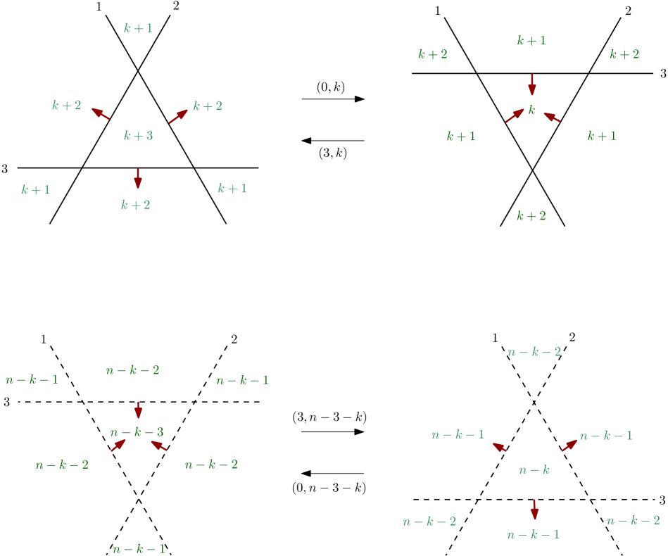
Figure 1: A mutation of Type $(0,k)\equiv(3,n-3-k)$ (from left to right), respectively $(3,k)\equiv(0,n-3-k)$ (from right to left) in $S^{2}$. The upper row shows the triangular faces $\sigma$ and $\tau$ before and after the mutation, and the lower row shows the corresponding antipodal faces $-\sigma$ and $-\tau$. The little arrows indicate positive halfspaces, and the labels in full-dimensional faces indicate levels.

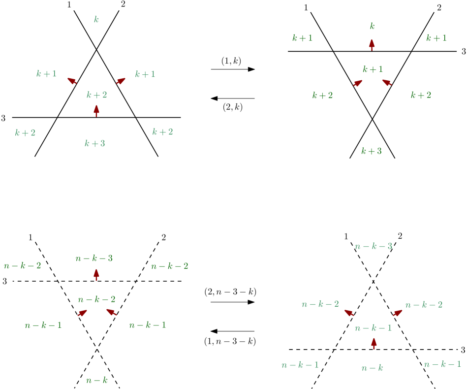
Figure 2: A mutation of Type $(1,k)\equiv(2,n-3-k)$ (from left to right), respectively $(2,k)\equiv(1,n-3-k)$ (from right to left) in $S^{2}$.

We are now ready to define the $g$-matrix $g(V\rightarrow W)$ of a pair of vector configurations.

Definition 3.2 ($g$-Matrix of a pair).

Let $V,W$ be configurations of $n$ vectors in $\mathbf{R}^{r}$.

If $V\to W$ is a single mutation of Type $(i,\ell)\equiv(r-i,n-r-\ell)$ then we define the $g$-matrix $g(V\rightarrow W)=[g_{j,k}(V\rightarrow W)]$, $0\leqslant j\leqslant r$ and $0\leqslant k\leqslant n-r$, as follows:

If $2i=r$ or $2\ell=n-r$, then $g_{j,k}(V\to W)=0$ for all $j,k$. If $2i\neq r$ and $2\ell\neq n-r$, then

$$g_{j,k}(V\to W):=\begin{cases}+1&\textrm{if }(j,k)=(i,\ell)\textrm{ or }(j,k)=(r-i,n-r-\ell)\\ -1&\textrm{if }(j,k)=(r-i,\ell)\textrm{ or }(j,k)=(i,n-r-\ell)\\ 0&\textrm{else.}\end{cases}$$

More generally, if $V$ and $W$ are connected by a sequence $V=V_{0},V_{1},\dots,V_{N}=W$, where $V_{s-1}$ and $V_{s}$ differ by a single mutation, then we define

$$g_{j,k}(V\to W):=\sum_{s=1}^{N}g_{j,k}(V_{s-1}\to V_{s})$$

Proof 3.3 (Proof of Thm 1.5).

All three properties follow directly from Definition 3.2 and Lemma 3.1.

A priori, it may seem that the definition of the $g$-matrix depends on the choice of a particular sequence of mutations transforming $V$ to $W$. However, this is not the case:

Lemma 3.4.

Let $f(x,y)=\sum_{s,t}f_{s,t}x^{s}y^{t}$ and $g(x,y)=\sum_{j,k}g_{j,k}x^{j}y^{k}$ be polynomials (with real coefficients $f_{s,t}$ and $g_{j,k}$ that are zero unless $0\leqslant s\leqslant d$ and $0\leqslant t\leqslant n$, respectively $0\leqslant j\leqslant r$ and $0\leqslant k\leqslant n-r$). Suppose that $f(x,y)$ and $g(x,y)$ satisfy the identity

$$f(x,y)=(1+x)^{r}g(\textstyle\frac{x+y}{1+x},y)=\sum_{j=0}^{r}\sum_{k=0}^{n-r}g_{j,k}\cdot(x+y)^{j}(1+x)^{r-j}y^{k}$$ (19)

Then, for every fixed $t$, the numbers $g_{j,t}$, $0\leqslant j\leqslant r$, are linear combinations of the numbers $f_{s,\ell}$, $0\leqslant s\leqslant d$ and $0\leqslant\ell\leqslant t$, with coefficients given inductively by the polynomial equations

$$\sum_{j}g_{j,t}x^{r-j}=\sum_{s}f_{s,t}(x-1)^{s}-\sum_{j}\sum_{k<t}g_{j,k}\binom{j}{t-k}x^{r-j}$$

Proof 3.5.

The coefficient of $y^{t}$ in $(x+y)^{j}(x+1)^{r-j}y^{k}$ equals $\binom{j}{t-k}(x+1)^{r-j}$ (which is zero unless $0\leqslant k\leqslant t$). Thus, fixing $t$ and collecting terms in (19) according to $y^{t}$, we get

$$\sum_{s}f_{s,t}x^{s}=\sum_{j}\sum_{k\leqslant t}g_{j,k}\binom{j}{t-k}(1+x)^{r-j}$$

Moving the terms with $k<t$ to the other side yields

$$\sum_{j}g_{j,t}(1+x)^{r-j}=\sum_{s}f_{s,t}x^{s}-\sum_{j}\sum_{k<t}g_{j,k}\binom{j}{t-k}(1+x)^{r-j}$$

The result follows by a change of variable from $x$ to $x-1$ (inductively, the numbers $g_{j,k}$, $k<t$, are determined by the numbers $f_{s,\ell}$, $\ell<t$.)

Proof 3.6 (Proof of Theorem 1.12).

By Theorem 2.10, the $f$-polynomial and the $f^{*}$-polynomial of a vector configuration determine each other. By combining this with Thm. 1.5, Theorem 1.12 follows.

We remark that Theorem 1.12 can also be proved directly, by studying how $\mathcal{F}^{*}$ changes during mutations. By Gale duality, Thms. 1.5 and 1.12 also imply the following:

Corollary 3.7.

Let $V,W\in\mathbf{R}^{r\times n}$ be vector configurations, and let $V^{*},W^{*}\in\mathbf{R}^{(n-r)\times n}$ be their Gale duals. Then $g_{j,k}(V\to W)=-g_{k,j}(V^{*}\to W^{*})$.

As an immediate application, we show that all neighborly configurations of $n$ vectors in $\mathbf{R}^{r}$ have the same $f$-matrix (hence the same $f^{*}$-matrix), and analogously for coneighborly configurations.

Proposition 3.8.

Let $V,W\in\mathbf{R}^{r\times n}$. Suppose that $V$ and $W$ are both coneighborly, or that both are neighborly. Then $g(V\to W)$ is identically zero, hence $f(V)=f(W)$, and $f^{*}(V)=f^{*}(W)$.

Proof 3.9.

If $V,W\in\mathbf{R}^{r\times n}$ are coneighborly configurations then $f_{s,t}(V)=f_{s,t}(W)=0$ for $t\leqslant\lfloor\frac{n-r-1}{2}\rfloor$. By Lemma 3.4, this implies that $g_{j,k}(V\to W)=0$ for $k\leqslant\lfloor\frac{n-r-1}{2}\rfloor$ and $0\leqslant j\leqslant r$. The skew-symmetry of the $g$-matrix then implies $g_{j,k}(V\to W)=0$ for all $j,k$. Thus, $f(V)=f(W)$ and $f^{*}(V)=f^{*}(W)$, by Thms. 1.5 and 1.12. The remaining statements follow by Gale duality.

3.2 Contractions and Deletions

Let $V=\{v_{1},\dots,v_{n}\}\subset\mathbf{R}^{r}$ be a vector configuration in general position. For $1\leqslant i\leqslant n$, consider the linear hyperplane $v_{i}^{\bot}\cong\mathbf{R}^{r-1}$ orthogonal to $v_{i}$, and let $V/v_{i}$ denote the vector configuration obtained by projecting the remaining vectors $v_{j}$, $j\neq i$, orthogonally onto $v_{i}^{\bot}$. Thus, $V/v_{i}$ is a configuration of $(n-1)$ vectors in rank $r-1$. In terms of the polar dual arrangements, $\mathcal{A}(V/i)$ is the intersection of the arrangement $\mathcal{A}(V)$ with the great $(d-1)$-sphere $H_{i}\cong S^{d-1}$ defined by $v_{i}$. We call $V/v_{i}$ a contraction.

Moreover, we call the configuration $V\setminus v_{i}$ of $n-1$ vectors in $\mathbf{R}^{r}$ obtained by removing $v_{i}$ a deletion. Deletions and contractions are Gale dual to each other, i.e., $(V/v_{i})^{*}=V^{*}\!\setminus\!v_{i}^{*}$.

Every generic continuous motion $V\to W$ between two vector configurations $V,W\in\mathbf{R}^{r\times n}$ in general position induces continuous motions $V/v_{i}\to W/w_{i}$ and $V\setminus v_{i}\to W\setminus w_{i}$, $1\leqslant i\leqslant n$.

Lemma 3.10 (Contractions and Deletions).

For $0\leqslant k\leqslant n-r$ and $0\leqslant j\leqslant r-1$,

$$\sum_{i=1}^{n}g_{j,k}(V/v_{i}\to W/w_{i})=(r-j)g_{j,k}(V\to W)+(j+1)g_{j+1,k}(V\to W)$$

Analogously, for $0\leqslant k\leqslant n-r-1$ and $0\leqslant j\leqslant r$,

$$\sum_{i=1}^{n}g_{j,k}(V\setminus v_{i}\to W\setminus w_{i})=(n-r-k)g_{j,k}(V\to W)+(k+1)g_{j,k+1}(V\to W)$$

Proof 3.11.

We prove the formula for contractions; the result for deletions follows by Gale duality. Consider the corresponding motion of arrangements in $S^{d}$. Consider a $(j,k)$-mutation in the full arrangement $\mathcal{A}(V)$, involving $r=d+1$ great $(d-1)$-spheres $H_{i}$, $i\in R$, for some $R\in\binom{[n]}{r}$, that pass through a common point during the mutation, and that bound a small simplex before and after the mutation. Let $J\in\binom{R}{j}$ be the set of indices such that the small simplex after the mutation is contained in $H_{i}^{-}$ for $i\in J$ and in $H_{i}^{+}$ for $i\in R\setminus J$. For each $i\in R$, we see a mutation in the arrangement restricted to $H_{i}\cong S^{d-1}$; this mutation in $S^{d-1}$ is of type $(j-1,k)$ if $i\in J$ and of type $(j,k)$ if $i\in R\setminus J$. For $i\in[n]\setminus R$, the restriction to $H_{i}$ does not undergo a mutation.

We say that a vector configuration $V\subset\mathbf{R}^{r}$ is $j$-neighborly if every subset of $V$ of size $j$ is extremal. We say that $V$ is $k$-coneighborly if $f_{s,t}=0$ for $t\leqslant k$, i.e., if every open linear halfspace contains at least $k+1$ vectors from $V$.

Lemma 3.12.

Let $0\leqslant j\leqslant\frac{r-1}{2}$, $0\leqslant k\leqslant\frac{n-r-1}{2}$, and let $V,W\in\mathbf{R}^{r\times n}$ be vector configurations such that $V$ is $k$-coneighborly and $W$ is $j$-neighborly. Then

$$\textstyle g_{j,k}(V\to W)=\binom{n-k-r+j}{j}\binom{k+r-1-j}{k}-\binom{n-k-r+j-1}{j-1}\binom{k+r-j}{k}>0$$ (20)

The proof, which we defer to Appendix A is by a double induction, using the deletion and contraction formulas from Lemma 3.10.

4 The Spaces $\mathfrak{G}_{n,r}$ and $\mathfrak{G}_{n,r}^{0}$ Spanned by $g$-Matrices

In this section, we prove Theorems 1.8, 1.9, and 1.13. By Theorems 1.5 and 1.12 and Lemma 3.4, the description of the spaces $\mathfrak{F}_{n,r}$, $\mathfrak{F}^{0}_{n,r}$, and $(\mathfrak{F}^{*}_{n,r})^{0}$ follows from the description of the spaces $\mathfrak{G}_{n,r}$ and $\mathfrak{G}_{n,r}^{0}$, so it remains to prove the latter.

Recall that $\mathcal{V}_{n,r}$ is the set of all vector configurations $V\in\mathbf{R}^{r\times n}$ in general position, and $\mathcal{V}_{n,r}^{0}$ the subset of pointed configurations.

By Theorem 1.5, the $g$-matrix $g=g(V\to W)$ of any pair $V,W\in\mathcal{V}_{n,r}$ satisfies the skew-symmetries $g_{j,k}=-g_{r-j,k}=-g_{j,n-r-k}=g_{r-j,n-r-k}$ in (6). Thus, in order to prove Theorem 1.8, it remains to show that $\mathfrak{G}_{n,r}=\lin\{g(V\to W)\colon V,W\in\mathcal{V}_{n,r}\}$ has dimension $\lfloor\frac{r+1}{2}\rfloor\lfloor\frac{n-r+1}{2}\rfloor$. To see this, consider a generic continuous deformation from a coneighborly configuration $V_{0}$ to a neighborly configuration $V_{N}$, and let $V_{t}$, $0\leqslant i\leqslant N$, be the intermediate vector configurations, i.e., $V_{t}$ and $V_{t-1}$ differ by a mutation. Thus, the $g$-matrices $g(V_{0}\to V_{t})$ and $g(V_{0}\to V_{t-1})$ differ by the $g$-matrix of a mutation, i.e., their first quadrants (small $g$-matrices) differ in at most one coordinate, by $+1$ or $-1$. Moreover, $g(V_{0}\to V_{0})$ is identically zero, and every entry of the first quadrant of $g(V_{0}\to V_{N})$ is strictly positive by Lemma 3.12. Thus, the proof of Theorem 1.8 is completed by the following lemma:

Lemma 4.1.

Let $X_{0},X_{1},\dots,X_{N}$ be vectors in $\mathbf{R}^{m}$ such that

1. $X_{0}=0$;

2. $X_{t}$ and $X_{t-1}$ differ in exactly one coordinate, by $+1$ or $-1$;

3. for every $1\leqslant i\leqslant m$, there exists $t$ such that $X_{t}$ and $X_{t-1}$ differ in the $i^{\text{th}}$ coordinate (e.g., this holds if all coordinates of $X_{N}$ are non-zero, by Conditions 1 and 2).

Then there is a subset $X_{t_{1}},\dots,X_{t_{m}}$ of vectors that form a basis of $\mathbf{R}^{m}$.

Proof 4.2.

For $1\leqslant i\leqslant m$, let $t_{i}$ be the smallest $t\in\{1,\dots,N\}$ such that the $i$-th coordinate of $X_{t_{i}}$ is non-zero; the index $t_{i}$ exists by Properties 1 and 3. Moreover, by Property 2, no two coordinates can become non-zero at the same time, i.e., the indices $t_{i}$ are pairwise distinct. Up to re-labeling the coordinates, we may assume $t_{1}<t_{2}<\ldots<t_{m}$. Then, for $1\leqslant i\leqslant m$, the vector $X_{t_{i}}$ is linearly independent from the vectors $X_{t_{1}},\dots X_{t_{i-1}}$, since all of the latter vectors have $i$-th coordinate zero. Thus, the $X_{t_{i}}$ form a basis.

In order to prove prove Theorems 1.9 and 1.13, we need to prove the description (10) of the space $\mathfrak{G}_{n,r}^{0}=\lin\{g(V\to W)\colon V,W\in\mathcal{V}^{0}_{n,r}\}$. We start by observing the following:

Lemma 4.3.

If $V,W\in\mathcal{V}^{0}_{n,r}$ then $g_{0,k}(V\to W)=0$ for all $k$.

Proof 4.4.

Up to a rotation, we may assume that both $V$ and $W$ are both contained in the same open halfspace $H^{+}=\{x\in\mathbf{R}^{r}\mid\langle u,x\rangle>0\}$, for some $u\in S^{d}$. Then $V$ can be deformed into $W$ through a continuous family $V(t)$ of vector configurations such that $V(t)\subset H^{+}$ and hence $0\notin\conv(V(t))$ for all $t$. Thus, there are no mutations of types $(0,k)$ for any $k$.

Thus, in order to prove (10), it remains to show that the space $\mathfrak{G}^{0}_{n,r}$ has dimension $\lfloor\frac{r-1}{2}\rfloor\lfloor\frac{n-r+1}{2}\rfloor$. To this end, by Lemma 4.1, it is enough to prove the following:

Lemma 4.5.

For every $n$ and $r$, there is a sequence $V_{0},V_{1},\ldots V_{N}$ of configurations in $\mathcal{V}^{0}_{n,r}$ with the following properties:

1. $V_{t}$ and $V_{t+1}$ differ by a single mutation,

2. For $1\leqslant j\leqslant\lfloor\frac{r-1}{2}\rfloor$, $0\leqslant k\leqslant\lfloor\frac{n-r-1}{2}\rfloor$, some mutation $V_{t-1}\to V_{t}$ is of Type $(j,k)$.

Consider a set $S=\{p_{1},\dots,p_{n}\}\subset\mathbf{R}^{d}$ in general position, corresponding to a pointed vector configuration $V=\{v_{1},\dots,v_{n}\}\subset\mathbf{R}^{d+1}$, where $v_{i}=(1,p_{i})$. In order to prove Lemma 4.5, we will construct a continuous deformation of the point set $S$ in $\mathbf{R}^{d}$ such that the corresponding continuous deformation of $V$ in $\mathbf{R}^{d+1}$ contains mutations of all types $(j,k)$, for $1\leqslant j\leqslant\lfloor\frac{d}{2}\rfloor$ and $0\leqslant k\leqslant\lfloor\frac{n-d-2}{2}\rfloor$.

Consider a set $Q=\{q_{1},\dots,q_{d}\}\subset\mathbf{R}^{d}$ of $d$ points in general position. We fix the labeling of the points by $i\in[d]$ and call $Q$ a labeled point set. Let $\Pi=\aff(Q)$ be the affine hyperplane spanned by $Q$. Every point $x\in\Pi$ can be uniquely written as an affine combination $x=\sum_{i=1}^{d}\alpha_{i}q_{i}$, $\alpha_{i}\in\mathbf{R}$, $\sum_{i}\alpha_{i}=1$. This defines, for every non-empty subset $\emptyset\neq\sigma\subset[d]$, a region $R_{\sigma}(Q)=\{\sum_{i=1}^{d}\alpha_{i}q_{i}\colon\sum_{i}\alpha_{i}=1,\alpha_{i}>0\textrm{ for }i\in\sigma,\alpha_{i}<0\textrm{ for }i\in[d]\setminus\sigma\}$ such that the union of the closures $\bigcup_{\emptyset\neq\sigma\subset[d]}\overline{R_{\sigma}(Q)}$ covers all of $\Pi$.

Let $S\subset\mathbf{R}^{d}$ be a set of $n$ points in general position, let $Q\subset S$ be a labeled subset of $d$ points, and let $p\in S\setminus Q$. Consider a continuous motion such that all points of $S\setminus\{p\}$ remain fixed and $p$ crosses the hyperplane $\Pi$ through the open region $R_{\sigma}(Q)$, from the halfspace $\Pi^{-}$ to the halfspace $\Pi^{+}$. Let $j=d-|\sigma|+1$ and $k=|\Pi^{+}\cap(S\setminus(Q\sqcup\{p\}))|$. Then this corresponds to a mutation of type $(j,k)\equiv(r-j,n-r-k)$ of the corresponding pointed vector configuration in $\mathbf{R}^{d+1}$.

Proof 4.6 (Proof of Lemma 4.5).

Let $A=\{a_{1},\dots,a_{d}\}\subset\mathbf{R}^{d}$ be a labeled point set in general position. For $\emptyset\neq\sigma\subseteq[d]$, choose a line $\ell_{\sigma}$ perpendicular to the affine hyperplane $\aff(A)$ that intersects $\aff(A)$ in a point in the open region $R_{\sigma}(A)$. Choose a small $d$-dimensional ball $B_{\varepsilon}$ of radius $\varepsilon>0$ centered at $a_{d}$. Let $q_{i}:=a_{i}$ for $1\leqslant i\leqslant d-1$. If we choose $\varepsilon$ sufficiently small, then for every $q_{d}\in B_{\varepsilon}$, the labeled set $Q=\{q_{1},\dots,q_{d}\}$ has the following property: For every $\emptyset\neq\sigma\subseteq[d]$, the line $\ell_{\sigma}$ intersects the hyperplane $\aff(Q)$ in the interior of the region $R_{\sigma}(Q)$.

Let us now set $p_{i}:=a_{i}$ for $1\leqslant i\leqslant d-1$, and choose $n-d$ points $p_{d},\dots,p_{n-1}\in B_{\varepsilon}$ such that $P:=\{p_{1},\dots,p_{n-1}\}\subset\mathbf{R}^{d}$ is in general position. These points will remain fixed throughout, and we refer to them as stationary.

Consider an additional point $p$ that moves continuously along one of the lines $\ell_{\sigma}$. During this continuous motion of $S=P\sqcup\{p\}$, we say that an interesting mutation occurs when $p$ crosses the affine hyperplane $\Pi=\aff(Q)$ spanned by some labeled $d$-element subset $Q\subset P$ of the form $Q=\{q_{1},\dots,q_{d}\}$ with $q_{i}=p_{i}$ for $1\leqslant i\leqslant d-1$, and $q_{d}\in P\setminus\{p_{1},\dots,p_{d-1}\}\subset B_{\varepsilon}$. By construction and by Observation 4, every interesting mutation is of type $(j,k)\equiv(r-j,n-r-k)$, where $j=d-|\sigma|+1$ is fixed and $k=|\Pi^{+}\cap P\setminus Q|$, where $\Pi^{+}$ is the open halfspace that $p$ enters. Thus, if we continuously move $p$ along $\ell_{\sigma}$ from one side of $\conv(P)$ to the other, then every value $0\leqslant k\leqslant n-1-d$ occurs at least once. We call this the $\ell_{\sigma}$-stage of the motion. We perform these $\ell_{\sigma}$-stages consecutively, for each of the lines $\ell_{\sigma}$, $\emptyset\neq\sigma\subseteq[d]$, in some arbitrary order, moving $p$ from one line to the next in between these stages in some arbitrary generic continuous motion. In the process, for every $(j,k)$ with $1\leqslant j\leqslant d$ and $0\leqslant k\leqslant n-1-d$, and interesting mutation of type $(j,k)$ will occur at least once. (We have no control over other, non-interesting mutations that occur both within the stages and in-between the different stages, but this is not necessary.)

Appendix A Proof of Lemma 3.12

We recall the statement that we wish to prove: Let $0\leqslant j\leqslant\frac{r-1}{2}$, $0\leqslant k\leqslant\frac{n-r-1}{2}$, and let $V,W\in\mathbf{R}^{r\times n}$ be vector configurations such that $V$ is $k$-coneighborly and $W$ is $j$-neighborly. Then

$$\textstyle g_{j,k}(V\to W)=\binom{n-k-r+j}{j}\binom{k+r-1-j}{k}-\binom{n-k-r+j-1}{j-1}\binom{k+r-j}{k}>0$$

We prove this by double induction. Let us first consider the case $j=0$, i.e., assume that $W$ is $0$-neighborly (i.e., pointed) and $V$ is $k$-coneighborly. We wish to show that

$$g_{0,k}(V\to W)=\binom{k+r-1}{r-1}=\binom{k+r-1}{k}$$ (21)

We show this by induction on $k$. Consider the base case where $V$ is $0$-coneighborly and $W$ is $0$-neighborly. Then $f_{0,0}(V)=0$ and $f_{0,0}(W)=1$, hence (using (9)), $g_{0,0}(V\to W)=f_{0,0}(W)-f_{0,0}(V)=1$. For the induction step, assume that $k\geqslant 1$. We use the deletion formulas from Lemma 3.10. Every deletion $V\setminus v_{i}$ is $(k-1)$-coneighborly, and every deletion $W\setminus w_{i}$ remains $0$-neighborly. Thus,

$$\underbrace{\sum_{i}g_{0,k-1}(V\setminus v_{i}\to W\setminus w_{i})}_{=n\binom{k-1+r-1}{k-1}}=(n-r-k+1)\underbrace{g_{0,k-1}(V\to W)}_{=\binom{k-1+r-1}{k-1}}+kg_{0,k}(V\to W)$$

hence $g_{0,k}(V\to W)=\frac{k+r-1}{k}\binom{k-1+r-1}{k-1}=\binom{k+r-1}{k}$, as we wanted to show.

For general $j$ and $k$, we now prove by induction on $j$ that

$$g_{\leqslant j,k}(V\to W)=\binom{n-k-r+j}{j}\binom{k+r-1-j}{k}$$ (22)

which implies (20). The base case $j=0$ is (21). Thus, assume that $j\geqslant 1$. We will use the contraction formulas from Lemma 3.10.

Claim 1.

$$g_{j,k}(V\to W)=\dfrac{1}{j}\Bigl{(}\sum_{i=1}^{n}g_{\leqslant j-1,k}(V/v_{i}\to W/w_{i})-r\cdot g_{\leqslant j-1,k}(V\to W)\Bigr{)}$$

Proof A.1.

By Lemma 3.10,

$$\sum_{i=0}^{n}g_{l-1,k}(V/v_{i}\to W/w_{i})=(r-l+1)\cdot g_{l-1,k}(V\to W)+l\cdot g_{l,k}(V\to W)$$ (23)

Summing up (23) for $1\leqslant l\leqslant j$, we get

$$\sum_{l=1}^{j}\sum_{i=1}^{n}g_{l-1,k}(V/v_{i}\to W/w_{i})=\sum_{l=1}^{j}(r-l+1)\cdot g_{l-1,k}(V\to W)+\sum_{l=1}^{j}l\cdot g_{l,k}(V\to W)$$

Thus,

$$\sum_{i=1}^{n}g_{\leqslant j-1,k}(V/v_{i}\to W/w_{i})=r\cdot g_{\leqslant j-1,k}(V\to W)\underbrace{-\sum_{l=1}^{j}(l-1)\cdot g_{l-1,k}(V\to W)}_{-\sum_{l=0}^{j-1}l\cdot g_{l,k}(V\to W)}+\sum_{l=1}^{j}l\cdot g_{l,k}(V\to W)$$

hence

$$\sum_{i=1}^{n}g_{\leqslant j-1,k}(V/v_{i}\to W/w_{i})=r\cdot g_{\leqslant j-1,k}(V\to W)+j\cdot g_{j,k}(V\to W)$$ (24)

as we claimed.

Every contraction $V/v_{i}$ is $(j-1)$-neighborly and every contraction $W/w_{i}$ remains $k$-coneighborly, hence, inductively,

$$g_{\leqslant j-1,k}(V/v_{i}\to W/w_{i})=\binom{n-k-r+j-1}{j-1}\binom{k+r-1-j}{k}$$

Moreover, also by induction $g_{\leqslant j-1,k}(V\to W)=\binom{n-k-r+j-1}{j-1}\binom{k+r-j}{k}$.

Substituting both into the formula from the claim, we get

$$g_{\leqslant j,k}(V\to W)=g_{\leqslant j-1,k}(V\to W)+g_{j,k}(V\to W)=\dfrac{n}{j}\cdot g_{\leqslant j-1,k}(V/v_{1}\to W/w_{1})-\dfrac{r-j}{j}\cdot g_{\leqslant j-1,k}(V\to W)=\\ =\dfrac{n}{j}\binom{n-k-r+j-1}{j-1}\binom{k+r-1-j}{k}-\frac{r-j}{j}\binom{n-k-r+j-1}{j-1}\binom{k+r-j}{k}=\\ =\dfrac{1}{j}\binom{n-k-r+j-1}{j-1}\left(n\binom{k+r-1-j}{k}-\underbrace{(r-j)\binom{k+r-j}{k}}_{\binom{k+r-j-1}{k}(k+r-j)}\right)=\\ =\underbrace{\dfrac{1}{j}\binom{n-k-r+j-1}{j-1}\Bigl{(}n-k-r+j\Bigr{)}}_{\binom{n-k-r+j}{j}}\binom{k+r-1-j}{k}$$ (25)

which proves (22).

It remains to show that $g_{j,k}(V\to W)>0$. For this, we rewrite (20) as

$$g_{j,k}(V\to W)=\underbrace{\binom{n-k-r+j}{j}}_{\binom{n-k-r+j-1}{j-1}\frac{n-k-r+j}{j}}\binom{k+r-1-j}{k}-\binom{n-k-r+j-1}{j-1}\underbrace{\binom{k+r-j}{k}}_{\binom{k+r-1-j}{k}\frac{k+r-j}{r-j}}\\ =\binom{n-k-r+j-1}{j-1}\binom{k+r-1-j}{k}\underbrace{\left(\frac{n-k-r+j}{j}-\frac{k+r-j}{r-j}\right)}_{>0}$$ (26)

To see that the expression in parentheses is positive, we notice $(n-k-r+j)(r-j)-j(k+r-j)=(n-k-r)(r-j)-jk$ and $n-k-r>k$, $r-j>j$ for the specified ranges of $j$ and $k$. This completes the proof of Lemma 3.12.∎

Appendix B A Proof of the Dehn–Sommerville Relations for Levels

The proof of the Dehn–Sommerville relations for levels in simple arrangements uses ideas closely related to the proof of Theorem 2.10. For completenes, we include the argument here.

Proof B.1 (Proof of Thm. 1.3).

Let $p(x,y,z):=\sum_{F\in\mathcal{F}(V)}x^{|F_{+}|}y^{|F_{-}|}z^{|F_{0}|}=x^{n}f_{V}(\frac{z}{x},\frac{y}{x})$ be the homogeneous version of the $f$-polynomial defined in the proof of Theorem 2.10.

Let $F,G\in\mathcal{F}(V)$ be the signatures of faces in $\mathcal{A}(V)$. We observe that the face with signature $F$ is contained in the face with signature $G$ iff $F\leqslant G$.

For every $G\in\mathcal{F}(V)$, the corresponding face combinatorially a polytope, hence its Euler characteristic equals $1=\sum_{F\in\mathcal{F}(V),F\leqslant G}(-1)^{d-|F_{0}|}$. Moreover, since the arrangement is simple, we get that for every $F\in\mathcal{F}(V)$, $\sum_{G\in\mathcal{F}(V),G\geqslant F}x^{|G_{+}|}y^{|G_{-}|}z^{|G_{0}|}=x^{|F_{+}|}y^{|F_{-}|}(x+y+z)^{|F_{0}|}$. Combining these two observations, we get

$$p(x,y,z) = \sum_{G\in\mathcal{F}(V)}x^{|G_{+}|}y^{|G_{-}|}z^{|G_{0}|}=\sum_{G\in\mathcal{F}(V)}\left(\sum_{F\in\mathcal{F}(V),F\leqslant G}(-1)^{d-|F_{0}|}\right)x^{|G_{+}|}y^{|G_{-}|}z^{|G_{0}|}$$

$$= (-1)^{d}\sum_{F\in\mathcal{F}(V)}(-1)^{|F_{0}|}\left(\sum_{G\in\mathcal{F}(V),G\geqslant F}x^{|G_{+}|}y^{|G_{-}|}z^{|G_{0}|}\right)$$

$$= (-1)^{d}\sum_{F\in\mathcal{F}(V)}x^{|F_{+}|}y^{|F_{-}|}(x+y+z)^{|F_{0}|}(-1)^{|F_{0}|}=(-1)^{d}p(x,y,-(x+y+z))$$

Thus, by (14), $f_{V}(x,y)=p(1,y,x)=(-1)^{d}p(1,y,-(x+y+1))=(-1)^{d}f_{V}(-(x+y+1),y).$

References

- [1] Artur Andrzejak, Boris Aronov, Sariel Har-Peled, Raimund Seidel, and Emo Welzl. Results on -sets and -facets via continuous motion. In Proceedings of the Fourteenth Annual Symposium on Computational Geometry, SCG ’98, pages 192–199, New York, NY, USA, 1998. Association for Computing Machinery.
- [2] Artur Andrzejak and Emo Welzl. In between -sets, -facets, and -faces: -partitions. Discrete Comput. Geom., 29(1):105–131, 2003.
- [3] Ranita Biswas, Sebastiano Cultrera di Montesano, Herbert Edelsbrunner, and Morteza Saghafian. Depth in arrangements: Dehn-Sommerville-Euler relations with applications. J. Appl. Comput. Topol., 8(3):557–578, 2024.
- [4] Anders Björner, Michel Las Vergnas, Bernd Sturmfels, Neil White, and Günter M. Ziegler. Oriented matroids, volume 46 of Encyclopedia of Mathematics and its Applications. Cambridge University Press, Cambridge, second edition, 1999.
- [5] Jürgen Eckhoff. Helly, Radon, and Carathéodory type theorems. In Handbook of convex geometry, Vol. A, B, pages 389–448. North-Holland, Amsterdam, 1993.
- [6] Herbert Edelsbrunner. Algorithms in combinatorial geometry, volume 10 of EATCS Monographs on Theoretical Computer Science. Springer-Verlag, Berlin, 1987.
- [7] Branko Grünbaum. Convex polytopes, volume 221 of Graduate Texts in Mathematics. Springer-Verlag, New York, second edition, 2003.
- [8] T. Gulliksen and A. Hole. On the number of linearly separable subsets of finite sets in . Discrete Comput. Geom., 18(4):463–472, 1997.
- [9] Johann Linhart. The upper bound conjecture for arrangements of halfspaces. Beiträge Algebra Geom., 35(1):29–35, 1994.
- [10] Johann Linhart, Yanling Yang, and Martin Philipp. Arrangements of hemispheres and halfspaces. Discrete Math., 223(1-3):217–226, 2000.
- [11] Jiří Matoušek. Lectures on discrete geometry, volume 212 of Graduate Texts in Mathematics. Springer-Verlag, New York, 2002.
- [12] Ketan Mulmuley. Dehn-sommerville relations, upper bound theorem, and levels in arrangements. In Chee Yap, editor, Proceedings of the Ninth Annual Symposium on Computational Geometry (San Diego, CA, USA, May 19-21, 1993), pages 240–246, 1993.
- [13] Elizaveta Streltsova and Uli Wagner. Sublevels in arrangements and the spherical arc crossing number of complete graphs. Preprint, 2025.
- [14] Uli Wagner. -Sets and -facets. In Surveys on Discrete and Computational Geometry, volume 453 of Contemp. Math., pages 443–513. Amer. Math. Soc., Providence, RI, 2008.
- [15] E. Welzl. Entering and leaving -facets. Discrete Comput. Geom., 25(3):351–364, 2001.
- [16] Günter M. Ziegler. Lectures on polytopes, volume 152 of Graduate Texts in Mathematics. Springer-Verlag, New York, 1995.