Counting 5-isogenies of elliptic curves over $\mathbb{Q}$

Abstract.

We show that the number of $5$-isogenies of elliptic curves defined over $\mathbb{Q}$ with naive height bounded by $H>0$ is asymptotic to $C_{5}\cdot H^{1/6}(\log H)^{2}$ for some explicitly computable constant $C_{5}>0$. This settles the asymptotic count of rational points on the genus zero modular curves $X_{0}(m)$. We leverage an explicit $\mathbb{Q}$-isomorphism between the stack $\mathscr{X}_{0}(5)$ and the generalized Fermat equation $x^{2}+y^{2}=z^{4}$ with $\mathbb{G}_{m}$-action of weights $(4,4,2)$.

1. Introduction

1.1. Setup: arithmetic statistics of elliptic curves

Let $E$ be an elliptic curve defined over $\mathbb{Q}$. Then $E$ is isomorphic to a unique elliptic curve $E_{A,B}$ with Weierstrass equation of the form

$$y^{2}=x^{3}+Ax+B,$$

where $A,B$ are integers, the discriminant $\Delta(A,B)\colonequals-16(4A^{3}+27B^{2})$ is nonzero, and no prime $\ell$ satisfies $\ell^{4}\mid A$ and $\ell^{6}\mid B$.

Let $\mathcal{E}$ denote the set of such elliptic curves. The naive height of $E\cong E_{A,B}\in\mathcal{E}$ is defined by

(1.1) $$\operatorname{Ht}(E)\colonequals\operatorname{Ht}(E_{A,B})\colonequals\max(4|A|^{3},27|B|^{2}).$$

For $H\geq 1$, define

(1.2) $$\mathcal{E}_{\leq H}\colonequals\{E\in\mathcal{E}:\operatorname{Ht}(E)\leq H\}.$$

Recent work has resolved many instances of counting problems for elliptic curves equipped with additional level structure as $H\to\infty$. For instance, Harron–Snowden [19] and Cullinan–Kenney–Voight [8], building on work by Duke [13] and Grant [18], provided asymptotics for the count of $E\in\mathcal{E}_{\leq H}$ where the torsion subgroup $E(\mathbb{Q})_{\mathrm{tors}}$ of the Mordell–Weil group is isomorphic to a given finite abelian group, for each of the 15 groups described in Mazur’s torsion theorem [24, Theorem 2]. These cases correspond to genus zero modular curves $Y_{1}(m)$ with infinitely many rational points.

Parallel to these cases, a family of modular curves that has received much attention is the classical modular curves $Y_{0}(m)$. Rational points on these curves correspond to isomorphism classes of rational cyclic $m$-isogenies. Explicitly, such an object can be thought of as a pair $(E,C)$ where $E$ is an elliptic curve defined over $\mathbb{Q}$, and $C\subset E(\bar{\mathbb{Q}})$ is a cyclic subgroup of order $m$ that is stable under the action of the absolute Galois group. Two such pairs $(E,C)$ and $(E^{\prime},C^{\prime})$ are said to be $\mathbb{Q}$-isomorphic, if there exists an isomorphism $\varphi\colon E\to E^{\prime}$ of elliptic curves, defined over $\mathbb{Q}$, such that $\varphi(C)=C^{\prime}$. Let $\mathcal{E}_{m}\colonequals Y_{0}(m)(\mathbb{Q})$ denote the set of isomorphism classes $[E,C]$ of rational cyclic $m$-isogenies, and consider the finite subsets

$$\mathcal{E}_{m,\leq H}\colonequals\mathopen{}\mathclose{{\left\{[E,C]\in\mathcal{E}_{m}:\operatorname{Ht}(E)\leq H}}\right\}.$$

As a corollary of Mazur’s Isogeny Theorem [24, Theorem 1], it is known that $Y_{0}(m)$ has infinitely many rational points if and only if

(1.3) $$m\in\mathopen{}\mathclose{{\left\{1,2,3,4,5,6,7,8,9,10,12,13,16,18,25}}\right\}.$$

These are precisely the levels $m$ for which the compactified curve $X_{0}(m)$ has genus zero.

1.2. Results

By recent work of several authors (see Table 1), the asymptotic order of growth of the counting function $N_{m}(H)\colonequals\#\mathcal{E}_{m,\leq H}$ was computed for every $m$ in this list, except for the stubborn level $m=5$, which had eluded all previous attempts. Our main theorem provides the asymptotic count of $5$-isogenies of elliptic curves.

Theorem 1.1.

There exist explicitly computable constants $C_{5},C_{5}^{\prime},C_{5}^{\prime\prime}\in\mathbb{R}$ and $c_{5}\in(0,1)$ such that

$$N_{5}(H)=C_{5}H^{1/6}(\log H)^{2}+C_{5}^{\prime}H^{1/6}(\log H)+C_{5}^{\prime\prime}H^{1/6}+O(H^{1/6}\cdot(\log H)^{-c_{5}}),$$

as $H\to\infty$. Furthermore, the constant $C_{5}$ is given by

(1.4) $$C_{5}=\frac{41}{1536\pi}\cdot V_{5}\cdot g_{1},$$

where $V_{5}$ is given by Equation 5.17, and $g_{1}$ is given by Equation 1.6.

Remark 1.2.

The nature of our methods prevent us from obtaining a power-saving error term for $N_{5}(H)$. We believe the error term can be improved to $O_{\varepsilon}(H^{1/12+\varepsilon})$.

In an upcoming paper by Alessandro Languasco and Pieter Moree [22], and independently by Steven Charlton, have numerically estimated the constants $V_{5}$ and $g_{1}$ to extremely high precision, from which we can obtain

(1.5) $$C_{5}\approx 0.00034377729776664529\dots$$

The previous best known estimate was $N_{5}(H)\asymp H^{1/6}(\log H)^{2}$ by work of Bogges–Sankar [7, Proposition 5.14]. Our strategy was inspired by their idea of exploiting explicit presentations for the ring of modular forms of $\Gamma_{0}(5)$. In fact, we refine their estimate and show that Theorem 1.1 is essentially equivalent to the following.

Theorem 1.3 (Theorem 3.2).

Let $N_{\mathscr{G}}(H)$ denote the counting function of the integer triples $(a,b,c)$ satisfying the following properties:

• $a^{2}+b^{2}=c^{4}$,

• $\gcd(a,b)$ is $4^{\text{th}}$-power free, and

• $|c|\leq H$.

Then, there exist explicitly computable constants $g_{1},g_{2},g_{3}\in\mathbb{R}$ such that for every $\varepsilon>0$, we have

$$N_{\mathscr{G}}(H)=g_{1}H(\log H)^{2}+g_{2}H(\log H)+g_{3}H+O_{\varepsilon}(H^{1/2+\varepsilon}),$$

as $H\to\infty$. Furthermore, the constant $g_{1}$ is given by the Euler product

(1.6) $$g_{1}=\frac{48}{\pi^{4}}\prod_{p\,\equiv\,1\text{ mod }4}\Bigl{(}1-\frac{4}{(p+1)^{2}}\Bigr{)}.$$

Languasco and Moree [22] have numerically estimated the constant $g_{1}$ to extremely high precision, obtaining

(1.7) $$g_{1}\approx 0.41662592496198471660\dotsc.$$

Adding our main result to the list, we now know the leading terms in the asymptotic counts of rational points for the genus zero modular curves $X_{0}(m)$.

Theorem 1.4.

Suppose that $m$ is in the list (1.3). Then, there exist explicitly computable constants $C_{m}\in\mathbb{R}_{>0}$, $a_{m}\in\mathbb{Q}_{\geq 0}$, and $b_{m}\in\mathbb{Z}_{\geq 0}$ such that

$$N_{m}(H)\sim C_{m}H^{a_{m}}(\log H)^{b_{m}}.$$

Moreover, the values of $a_{m}$ and $b_{m}$ are presented in Table 1.

Table 1. Powers of $H$ and $\log H$ in the main terms in the asymptotic of the counting functions $N_{m}(H)$.

$m$	$a_{m}$	$b_{m}$	Reference
1	5/6	0	[6, Lemma 4.3]
2	1/2	0	[18, Proposition 1]
3	1/2	0	[29, Theorem 1.3]
4	1/3	0	[30, Theorem 4.2]
5	1/6	2	Theorem 1.1
6	1/6	1	[25, Theorem 7.3.14]
7	1/6	1	[26, Theorem 1.2.2]
8	1/6	1	[25, Theorem 7.3.14]
9	1/6	1	[25, Theorem 7.3.14]
10	1/6	0	[25, Theorem 5.4.11]
12	1/6	1	[25, Theorem 7.3.18]
13	1/6	0	[25, Theorem 6.4.5]
16	1/6	1	[25, Theorem 7.3.18]
18	1/6	1	[25, Theorem 7.3.18]
25	1/6	0	[25, Theorem 5.4.11]

Remark 1.5.

Since some elliptic curves admit multiple non isomorphic cyclic $m$-isogenies, the problem of counting elliptic curves that admit an isogeny is related but distinct. In particular, [25] denotes our counting function by $\widetilde{N}_{m}(H)$. For $m=5$, a single elliptic curve $E$ can admit at most two distinct $\mathbb{Q}$-rational $5$-isogenies. See [9].

Remark 1.6.

For both torsion and isogenies, the work of Bruin–Najman [5] and Phillips [28] extend these asymptotic counts to the case of number fields when the corresponding moduli stack is a weighted projective line.

For $m\neq 5$, the strategy was roughly the following. Use a rational parametrization $\mathbb{P}^{1}\cong X_{0}(m)$ to find polynomial equations $A_{m}(t)$ and $B_{m}(t)$ for the Weierstrass coefficients of elliptic curves admitting a rational cyclic $m$-isogeny. Homogenize these polynomials to turn the estimation of $N_{m}(H)$ into a lattice point counting problem in the compact region

$$R_{m,\leq H}\colonequals\mathopen{}\mathclose{{\left\{(x,y)\in\mathbb{R}^{2}:\max(4|A_{m}(x,y)|^{3},27B_{m}(x,y)^{2})\leq H}}\right\},$$

and use the principle of Lipschitz and a careful sieve to conclude the results. This approach is sufficient when the expected power of $\log H$ in the main term of $N_{m}(H)$ is $b_{m}=0$. This is not surprising, since the main term predicted by the principle of Lipschitz is the area of the region $R_{m,\leq H}$, which is $\asymp H^{a}$.

Notably, Molnar–Voight [26] where able to salvage this approach to show that

$$N_{7}(H)\sim C_{7}H^{1/6}(\log H).$$

They observed that counting $7$-isogenies up to $\bar{\mathbb{Q}}$-isomorphism has the effect of removing the $\log H$ factor, which allowed them to use Lipschitz for this rigidified count, and then recover the full count by precisely estimating the number of twists with a given height (see [26, Theorem 5.1.4]).

Unfortunately, this rigidification method is not enough to count $5$-isogenies essentially because we can only remove one factor of $\log H$. Nevertheless, we use their rigidification method to simplify the calculations. For a detailed discussion of why this method fails for $m=5$, see Remark 1.3.2 and Remark 5.3.53 in Molnar’s Ph.D. thesis [25].

1.3. Sketch of the proof

Our approach does not use a rational parametrization of $X_{0}(5)$. Instead, we leverage an explicit embedding of the moduli stack $\mathscr{X}_{0}(5)$ in weighted projective space. This allows us to parametrize $5$-isogenies in terms of (4,4,2)-minimal integral solutions to the generalized Fermat equation $x^{2}+y^{2}=z^{4}$. (An integer triple $(a,b,c)$ is (4,4,2)-minimal, if there is no prime $\ell$ satisfying $\ell^{4}\mid a$, $\ell^{4}\mid b$, and $\ell^{2}\mid c$).

Remark 1.7 (Ignoring stacks).

Keeping stacks in the back of one’s mind is enlightening but not crucial for reading this article. If the reader wishes to understand our proof while ignoring stacks completely, they can safely skip Section 2.

Remark 1.8 (Embracing stacks).

The stacky perspective offers a conceptual framework ideally suited to studying counting problems of this nature. The ideas presented in Section 2 are applicable in other contexts and might provide some insight into the Batyrev–Manin–Malle conjectures for rational points on stacks as in [17],[14], [23].

We break the proof into four steps and dedicate one section to each one.

1. In Section 2, we study the geometry of the moduli stack $\mathscr{X}_{0}(5)$ (defined over $\mathbb{Q}$) with coarse space $X_{0}(5)$. We show that $\mathscr{X}_{0}(5)$ is $\mathbb{Q}$-isomorphic to the closed substack of the weighted projective stack $\mathscr{P}(4,4,2)$ with equation $x^{2}+y^{2}=z^{4}$. The key result of this section towards the proof of our main theorem is Lemma 2.8.

2. In Section 3, we count $(4,4,2)$-minimal Gaussian integers with bounded norm. We use a zeta function approach and the factorization method, as explained in [3].

3. In Section 4, we prove the Main analytic lemma (Lemma 4.2). This enables us to count integral ideals in the Gaussian integers with numerical norm inside a homogeneously expanding region $\Omega$, as long as $\Omega$ is similar enough to a square. This section resides in the realm of complex analysis, and is independent from the rest of the article.

4. In Section 5 we feed our parametrization of $5$-isogenies and the count of $(4,4,2)$-minimal Gaussian integers of bounded norm into the Main analytic lemma, completing the proof of Theorem 1.1.

Acknowledgments

We sincerely thank the organizers of 2023 AMS Mathematics Research Communities, Explicit Computations with Stacks, for providing a wonderful environment from which this collaborative project started. This project is generously supported by the National Science Foundation Grant Number 1916439 for the 2023 Summer AMS Mathematics Research Communities. We thank John Voight for getting this project started and for sharing his code to compute canonical rings. We thank David Zureick-Brown, and Jordan Ellenberg for helpful conversations about this project. We thank Robert Lemke Oliver for suggesting the approach presented in Section 4. We thank Alessandro Languasco and Pieter Moree for their insightful comments on an earlier draft, and for sharing their computations with us. We thank Steven Charlton for sharing his computations with us. C.H. is very grateful to Korea University Grants K2422881, K2424631, K2510471, and K2511121 for the partial financial support. O.P. and S.W.P are very grateful to the Max-Planck-Institut für Mathematik Bonn for their hospitality and financial support.

2. Embedding $\mathscr{X}_{0}(5)$ into $\mathscr{P}(4,4,2)$

We work in the level of generality required for our applications. In particular, the geometric objects in this section are defined over $\mathbb{Q}$.

2.1. The stacky proj construction

We recall the stacky proj construction [27, Example 10.2.8], specializing to the case where the base scheme is $\operatorname{Spec}\mathbb{Q}$. Given a graded $\mathbb{Q}$-algebra $R=\bigoplus_{d\geq 0}R_{d}$, the multiplicative group $\mathbb{G}_{m}$ acts on $\operatorname{Spec}R$. The action is determined by the grading, and it fixes the point $0\colonequals V(R_{+})$ corresponding to the irrelevant ideal $R_{+}\colonequals\bigoplus_{d>0}R_{d}$. Define the stacky proj of $R$ to be the quotient stack

$$\operatorname{\mathbf{Proj}}R\colonequals[(\operatorname{Spec}R-0)/\mathbb{G}_{m}].$$

The stack $\operatorname{\mathbf{Proj}}R$ admits a coarse space, namely the scheme $\operatorname{Proj}R$. Moreover, if $R$ is generated in degree one, then $\operatorname{\mathbf{Proj}}R=\operatorname{Proj}R$.

Example 2.1 (The moduli stack of elliptic curves).

Consider the graded algebra $\mathbb{Q}[u^{4}\mathsf{x},u^{6}\mathsf{y}]$, where the grading is determined by the dummy variable $u$. By definition, the weighted projective line $\mathscr{P}(4,6)$ is $\operatorname{\mathbf{Proj}}\mathbb{Q}[u^{4}\mathsf{x},u^{6}\mathsf{y}]$. Using Weierstrass equations, one can show that $\mathscr{P}(4,6)$ is isomorphic to the moduli stack $\mathscr{X}(1)$ of stable elliptic curves over $\mathbb{Q}$. In particular, the groupoid of rational points $\mathscr{X}(1)(\mathbb{Q})$ is equivalent to the groupoid $\mathscr{P}(4,6)(\mathbb{Q})$ with

• Objects: pairs $(A,B)\in\mathbb{Q}\times\mathbb{Q}-(0,0)$.

• Isomorphisms: elements $\lambda\in\mathbb{Q}^{\times}$, sending $(A,B)\mapsto(\lambda^{6}A,\lambda^{4}B)$.

Example 2.2.

Consider the graded algebra $R\colonequals\mathbb{Q}[u^{4}\mathsf{x},u^{4}\mathsf{y},u^{2}\mathsf{z}]/(u^{8}(\mathsf{x}^{2}+\mathsf{y}^{2}-\mathsf{z}^{4}))$, and let $\mathscr{G}\colonequals\operatorname{\mathbf{Proj}}R$. The quotient map $\mathbb{Q}[u^{4}\mathsf{x},u^{4}\mathsf{y},u^{2}\mathsf{z}]\to R$ induces a closed embedding $\mathscr{G}\hookrightarrow\mathscr{P}(4,4,2)$. We will show that $\mathscr{G}$ is isomorphic to the moduli space $\mathscr{X}_{0}(5)$ of generalized elliptic curves together with $5$-isogenies. In particular, the groupoid of rational points $\mathscr{X}_{0}(5)(\mathbb{Q})$ is equivalent to the groupoid $\mathscr{G}(\mathbb{Q})$ with

• Objects: triples $(a,b,c)\in\mathbb{Q}\times\mathbb{Q}\times\mathbb{Q}-(0,0,0)$ satisfying $a^{2}+b^{2}=c^{4}$.

• Isomorphisms: elements $\lambda\in\mathbb{Q}^{\times}$, sending $(a,b,c)\mapsto(\lambda^{4}a,\lambda^{4}b,\lambda^{2}c)$.

We now explain special properties of $\operatorname{Proj}R$ that are mentioned in [2, Section 2]. When the graded $\mathbb{Q}$-algebra $R$ satisfies $R_{0}=\mathbb{Q}$, the stack $\operatorname{\mathbf{Proj}}R$ is special, as the stabilizers of any point of $\operatorname{\mathbf{Proj}}R$ is a finite subgroup of $\mathbb{G}_{m}$. If in addition $R$ is a finitely generated graded $\mathbb{Q}$-algebra, then $\operatorname{\mathbf{Proj}}R$ is an example of a cyclotomic stack (see [2, Definition 2.3.1]). Just like $\operatorname{\mathbf{Proj}}R$, any cyclotomic stack $\mathscr{X}$ has a coarse moduli space $X$. Note that both $\mathscr{X}(1)$ and $\mathscr{G}$ from Example 2.1 and Example 2.2 are cyclotomic stacks.

Recall that if the graded $\mathbb{Q}$-algebra $R$ is finitely generated by elements of $R_{1}$ and $R_{0}=\mathbb{Q}$, then there is a closed immersion $\operatorname{Proj}R\hookrightarrow\mathbb{P}R_{1}\colonequals\operatorname{Proj}\operatorname{Sym}R_{1}$. In this case, the line bundle $\mathcal{O}_{\operatorname{Proj}R}(1)=\mathcal{O}_{\mathbb{P}R_{1}}(1)|_{\operatorname{Proj}R}$ can be recovered from the graded $R$-module $R(1)$. Similarly, if $R_{0}=\mathbb{Q}$ but $R$ is not necessarily generated by $R_{1}$, then $\operatorname{\mathbf{Proj}}R$ is equipped with a line bundle $\mathcal{O}_{\operatorname{\mathbf{Proj}}R}(1)$; the pullback of $\mathcal{O}_{\operatorname{\mathbf{Proj}}R}(1)$ via $\operatorname{Spec}R-0\to\operatorname{\mathbf{Proj}}R$ is the $\widetilde{R(1)}|_{\operatorname{Spec}R-0}$, where $\widetilde{R(1)}$ is the sheaf associated to the graded $R$-module $R(1)$. Note that $\mathbb{G}_{m}$ acts faithfully on the line bundle $\widetilde{R(1)}|_{\operatorname{Spec}R-0}$ over the $\mathbb{G}_{m}$-variety $\operatorname{Spec}R-0$. Consequently, the stabilizer groups of any point of $\operatorname{\mathbf{Proj}}R$ act faithfully on the corresponding fiber of $\mathcal{O}_{\operatorname{\mathbf{Proj}}R}(1)$; such a line bundle is called a uniformizing line bundle (see [2, Definition 2.3.11]).

Just as $\mathcal{O}_{\operatorname{Proj}R}(1)$ is an ample line bundle on $\operatorname{Proj}R$, $\mathcal{O}_{\operatorname{\mathbf{Proj}}R}(1)$ is more than just a uniformizing line bundle.

Definition 2.3 ([2, Definition 2.4.1]).

Suppose that $\mathscr{X}$ is a proper cyclotomic $\mathbb{Q}$-stack with coarse moduli space $X$. Denote by $c\colon\mathscr{X}\to X$ the coarse map. Then a uniformizing line bundle $\mathcal{L}$ on $\mathscr{X}$ is called a polarizing line bundle if there exists an ample line bundle $M$ on $X$ and a positive integer $e$ such that $\mathcal{L}^{e}\cong c^{*}M$.

We claim that if $R$ is a finitely generated graded $\mathbb{Q}$-algebra such that $R_{0}=\mathbb{Q}$ and $R_{1,m}\colonequals\oplus_{1\leq d\leq m}R_{d}$ generates $R$, then the uniformizing line bundle $\mathcal{O}_{\operatorname{\mathbf{Proj}}R}(1)$ is a polarizing line bundle; this claim immediately implies that $\mathcal{O}_{\mathscr{X}(1)}(1)$ and $\mathcal{O}_{\mathscr{G}}(1)$ are polarizing line bundles on $\mathscr{X}(1)$ and $\mathscr{G}$, respectively. To see this, recall that $\operatorname{Proj}R$ is a closed subscherme of a weighted projective space $\mathbb{P}R_{1,m}\colonequals\operatorname{Proj}R^{\prime}$, where $R^{\prime}$ is a free graded $\mathbb{Q}$-algebra generated by the graded $\mathbb{Q}$-vector space $R_{1,m}$; note that $R$ is a graded quotient of $R^{\prime}$. Then, there exists a positive integer $e$ such that $\mathcal{O}_{\mathbb{P}R_{1,m}}(e)|_{\operatorname{Proj}R}$ is a line bundle on $\operatorname{Proj}R$, which implies that $\mathcal{O}_{\operatorname{\mathbf{Proj}}R}(e)\cong c^{*}(\mathcal{O}_{\mathbb{P}R_{1,m}}(e)|_{\operatorname{Proj}R})$; here, $e$ is not necessarily equal to $1$ as $\mathcal{O}_{\mathbb{P}R_{1,m}}(k)$ may not be locally free for some values of $k$.

2.2. Rigidification

Recall the notion of rigidification, as presented for instance in [1, Appendix C]. When $\mathscr{X}=\operatorname{\mathbf{Proj}}R$, the rigidification construction is very explicit. Indeed, let $d$ be the greatest common divisor of the degrees of the generators of $R$, so that $R=\bigoplus_{n\geq 0}R_{nd}$. Note that $\mu_{d}\colonequals\operatorname{Spec}\mathbb{Q}[t]/(t^{d}-1)\subset\mathbb{G}_{m}$ acts trivially on $\operatorname{Spec}R$. Consider the graded ring $S\colonequals\bigoplus_{n\geq 0}S_{n}$ defined by $S_{n}\colonequals R_{nd}$. We have a homomorphism $S\to R$ which is the identity at the level of rings, but multiplies the degree of every homogeneous element of $S$ by $d$. Then, the corresponding morphism of stacks $\operatorname{\mathbf{Proj}}R\to\operatorname{\mathbf{Proj}}S$ is a $\mu_{d}$-gerbe, and $\mathscr{X}\mathbin{\!\!\boldsymbol{\fatslash}}\mu_{d}=\operatorname{\mathbf{Proj}}S$ is the rigidification of $\mathscr{X}$ by $\mu_{d}$-inertia. In this case, the pullback of $\mathcal{O}_{\operatorname{\mathbf{Proj}}S}(1)$ under the rigidification $\operatorname{\mathbf{Proj}}R\to\operatorname{\mathbf{Proj}}S$ is $\mathcal{O}_{\operatorname{\mathbf{Proj}}R}(d)$.

Example 2.4 (The rigidified moduli space of elliptic curves).

The rigidification $\mathscr{Z}(1)\colonequals\mathscr{X}(1)\mathbin{\!\!\boldsymbol{\fatslash}}\mu_{2}$ is isomorphic to $\mathscr{P}(2,3)$. In particular, the groupoid of rational points $\mathscr{Z}(1)(\mathbb{Q})$ is equivalent to the groupoid $\mathscr{P}(2,3)(\mathbb{Q})$ with

• Objects: pairs $(A,B)\in\mathbb{Q}\times\mathbb{Q}-(0,0)$.

• Isomorphisms: elements $\lambda\in\mathbb{Q}^{\times}$, sending $(A,B)\mapsto(\lambda^{2}A,\lambda^{3}B)$.

Example 2.5.

The rigidification of the graded $\mathbb{Q}$-algebra $R$ from Example 2.2 is $S\colonequals\mathbb{Q}[u^{2}\mathsf{x},u^{2}\mathsf{y},u\mathsf{z}]/(u^{4}(\mathsf{x}^{2}+\mathsf{y}^{2}-\mathsf{z}^{4}))$. Let $\mathscr{F}\colonequals\operatorname{\mathbf{Proj}}S$. Then $\mathscr{G}\to\mathscr{F}$ is a $\mu_{2}$-gerbe, and $\mathscr{F}$ is the rigidification of $\mathscr{G}$. We will show that $\mathscr{F}$ is isomorphic to $\mathscr{Z}_{0}(5)\colonequals\mathscr{X}_{0}(5)\mathbin{\!\!\boldsymbol{\fatslash}}\mu_{2}$. In particular, the groupoid of rational points $\mathscr{Z}_{0}(5)(\mathbb{Q})$ is equivalent to the groupoid $\mathscr{F}(\mathbb{Q})$ with

• Objects: triples $(a,b,c)\in\mathbb{Q}\times\mathbb{Q}\times\mathbb{Q}-(0,0,0)$ satisfying $a^{2}+b^{2}=c^{4}$.

• Isomorphisms: elements $\lambda\in\mathbb{Q}^{\times}$, sending $(a,b,c)\mapsto(\lambda^{2}a,\lambda^{2}b,\lambda c)$.

2.3. Coordinate rings of stacky curves

A stacky curve is a smooth proper geometrically connected Deligne–Mumford stack, defined over a field, that contains a dense open subscheme (see [33, Chapter 5]). Let $\mathscr{X}$ be a stacky curve over $\mathbb{Q}$, and let $\mathcal{L}$ be a line bundle on $\mathscr{X}$. The homogeneous coordinate ring relative to $\mathcal{L}$ is the graded ring

(2.1) $$R_{\mathcal{L}}\colonequals\bigoplus_{d\geq 0}H^{0}(\mathscr{X},\mathcal{L}^{\otimes d}).$$

The degree $d$ piece of $R_{\mathcal{L}}$ is $R_{\mathcal{L},d}\colonequals H^{0}(\mathscr{X},\mathcal{L}^{\otimes d})$. When $\mathcal{L}\cong\mathcal{O}_{\mathscr{X}}(D)$ where $D$ is a Cartier divisor, we call $R_{D}\colonequals R_{\mathcal{L}}$.

Example 2.6.

Recall from Example 2.1 that $\mathscr{X}(1)\cong\operatorname{\mathbf{Proj}}\mathbb{Q}[u^{4}\mathsf{x},u^{6}\mathsf{y}]$. In fact, this isomorphism identifies the polarizing line bundle $\mathcal{O}_{\mathscr{X}}(1)$ with the Hodge bundle $\lambda$ on $\mathscr{X}(1)$, so that $\mathscr{X}(1)\cong R_{\lambda}$. Note that $R_{\lambda}=\mathbb{Q}[E_{4},E_{6}]$ is the ring of modular forms on the modular curve $\mathscr{X}(1)$ (with $\mathbb{Q}$-coefficients), where $E_{4}$ and $E_{6}$ are the Eisenstein series with constant term $1$ in their $q$-series expansion. Thus, $u^{4}\mathsf{x}$ is identified with $E_{4}$ and $u^{6}\mathsf{y}$ is identified with $E_{6}$ via the isomorphism $R_{\mathcal{O}_{\mathscr{X}(1)}(1)}\cong R_{\lambda}$.

For our calculations, we use the standard normalization of the Weierstrass coefficients $A=-3E_{4}$ and $B=-2E_{6}$.

If $\mathcal{L}$ is a polarizing line bundle on a cyclotomic stacky curve $\mathscr{X}$, then $\mathscr{X}$ can be recovered from $R_{\mathcal{L}}$ by the following slight extension of [2, Corollary 2.4.4].

Lemma 2.7.

Suppose that $\mathscr{X}$ is a proper geometrically connected cyclotomic $\mathbb{Q}$-stack with a polarizing line bundle $\mathcal{L}$. Then

$$\mathscr{X}\cong\operatorname{\mathbf{Proj}}R_{\mathcal{L}}.$$

Proof.

By the proof of [2, Proposition 2.3.10], $\mathscr{X}\cong[P_{\mathcal{L}}/\mathbb{G}_{m}]$, where the $\mathbb{G}_{m}$-torsor $P_{\mathcal{L}}\colonequals\mathscr{X}\times_{B\mathbb{G}_{m}}\operatorname{Spec}\mathbb{Q}$ on $\mathscr{X}$ is defined by the classifying morphism $\mathscr{X}\to B\mathbb{G}_{m}$ associated with $\mathcal{L}$. The proof of [2, Corollary 2.4.4] implies that $P_{\mathcal{L}}$ is an open subscheme of $\operatorname{Spec}R_{\mathcal{L}}$, so it suffices to show that $P_{\mathcal{L}}\cong\operatorname{Spec}R_{\mathcal{L}}-V(R_{\mathcal{L},+})$ by the definition of $\operatorname{\mathbf{Proj}}R_{\mathcal{L}}$.

Denote by $c\colon\mathscr{X}\to X$ the coarse map. Since $\mathcal{L}$ is a polarizing line bundle, there exists $e\in\mathbb{Z}_{+}$ and an ample line bundle $M$ on $X$ such that $\mathcal{L}^{e}\cong c^{*}M$. Connectedness of $\mathscr{X}$ implies that $R_{\mathcal{L},0}=\mathbb{Q}=R_{M,0}$. Then $X\cong[P_{M}/\mathbb{G}_{m}]$ is a projective scheme with an ample line bundle $M$, so that $P_{M}\cong\operatorname{Spec}R_{M}-V(R_{M,+})$. By the proof of [2, Corollary 2.4.4] again, $\operatorname{Spec}R_{\mathcal{L}}$ is isomorphic to the relative normalization of $\operatorname{Spec}R_{M}$ in $P_{\mathcal{L}}$ via a morphism $P_{\mathcal{L}}\to\operatorname{Spec}R_{M}$ factoring through $P_{M}$. As the induced morphism $P_{\mathcal{L}}\to P_{M}$ is a finite surjection by loc. cit., the induced inclusion $P_{\mathcal{L}}\hookrightarrow\operatorname{Spec}R_{\mathcal{L}}$ identifies $P_{\mathcal{L}}$ with $\operatorname{Spec}R_{\mathcal{L}}-V(R_{\mathcal{L},+})$, proving the desired assertion. ∎

For the remainder of this subsection, we apply Lemma 2.7 to describe a modular curve $\mathscr{X}_{0}(5)$ as a stacky Proj. Let the $\mathbb{Q}$-stack $\mathscr{X}_{0}(5)$ be the modular curve parameterizing generalized elliptic curves over $\mathbb{Q}$ with $\Gamma_{0}(5)$-structure, as in [32]. By [12, IV.6.7], the proper DM stack $\mathscr{X}_{0}(5)$ is a smooth stacky curve, and it admits a projection $J\colon\mathscr{X}_{0}(5)\to\mathscr{X}(1)$ which forgets the $\Gamma_{0}(5)$-structure on generalized elliptic curves. Using $J$, we identify $\mathscr{X}_{0}(5)$ with the stack $\mathscr{G}$ from Example 2.2.

Lemma 2.8.

The stacks $\mathscr{X}_{0}(5)$ and $\mathscr{G}$ are isomorphic. Consequently, so are their rigidifications $\mathscr{Z}_{0}(5)$ and $\mathscr{F}$.

Proof.

Recall from Example 2.6 that $\mathscr{X}(1)\cong\operatorname{\mathbf{Proj}}R_{\lambda}$, where $\lambda$ is the Hodge bundle on $\mathscr{X}(1)$ and $R_{\lambda}$ is the ring of modular forms on $\mathscr{X}(1)$. As $\lambda$ is a polarizing line bundle on $\mathscr{X}(1)$ and $J\colon\mathscr{X}_{0}(5)\to\mathscr{X}(1)$ is a finite surjection, $\mathscr{X}_{0}(5)$ is a geometrically connected proper cyclotomic stack equipped with a polarizing line bundle $J^{*}\lambda$. Thus, $\mathscr{X}_{0}(5)\cong\operatorname{\mathbf{Proj}}R_{J^{*}\lambda}$ by Lemma 2.7, and $R_{J^{*}\lambda}$ is the ring of modular forms on the modular curve $\mathscr{X}_{0}(5)$. The computations in the file abc-parametrization.m verify that the ring of modular forms $R_{J^{*}\lambda}$ is isomorphic, as graded $\mathbb{Q}$-algebras, to the ring $R$ from Example 2.2. As $\mathscr{G}\cong\operatorname{\mathbf{Proj}}R$, we see that $\mathscr{X}_{0}(5)$ and $\mathscr{G}$ are isomorphic. ∎

2.4. Geometric interpretation of the counting problem

There are significant recent advances ([17, 14, 15]) in systematically defining heights of stacks as a direct generalization of height functions on projective varieties. In [14, Definition 4.3], a height of a smooth DM stack $\mathscr{X}$ (with mild conditions as in [14, Definition 2.1]) is defined by a choice of a line bundle $\mathcal{L}$ on $\mathscr{X}$ together with a bounded function (determined by a raising datum in [14, Definition 4.1]). As a result, heights on $\mathscr{X}$ corresponding to the same line bundle $\mathcal{L}$ are $O(1)$-equivalent, as they only differ by the choice of bounded functions.

For the original counting problem (Theorem 1.1), the height function comes from the line bundle $J^{*}\lambda^{12}$ on $\mathscr{X}_{0}(5)$, where $J$ and $\lambda$ are as in Section 2.3. For the second counting problem (Theorem 1.3), the height commes from $\mathcal{O}_{\mathscr{G}}(2)$. The statement and the proof of Lemma 2.8 imply that $\mathcal{O}_{\mathscr{G}}\cong J^{*}\lambda$ on $\mathscr{G}\cong\mathscr{X}_{0}(5)$; so, the $6^{\rm th}$-power of the second height is $O(1)$-equivalent to the first height. This $O(1)$-equivalence turns out to be useful, as the lattice counting associated with $N_{5}(H)$ defined by the first height is complicated, whereas the lattice counting associated with $N_{\mathscr{G}}(H^{1/6})$ is much simpler; in fact, the region coming from $N_{\mathscr{G}}(H)$ is a disc.

However, the $O(1)$-equivalence does not guarantee that the counting functions have the same leading or lower-order terms, as predicted by the stacky Batyrev–Manin conjecture formulated in [14, §9.2] (also see weak form in [17, Conjecture 4.14]). To obtain $N_{5}(H)$ from $N_{G}(H)$, we will use heights on rigidified stacks $\mathscr{Z}_{0}(5)$ and $\mathscr{F}$ of $\mathscr{X}_{0}(5)$ and $\mathscr{G}$ respectively; Figure 1 summarizes the relations between the four stacks of interest.

Figure 1. This diagram summarizes the stacks considered in this paper and their respective coarse spaces. $C_{2}$ is the plane curve $\mathsf{x}^{2}+\mathsf{y}^{2}=\mathsf{z}^{2}$.

3. Counting minimal integer solutions to $x^{2}+y^{2}=z^{4}$

Recall that an integer triple $(a,b,c)$ is (4,4,2)-minimal if no prime $\ell$ satisfies $\ell^{4}\mid a,$ $\ell^{4}\mid b,$ and $\ell^{2}\mid c$; equivalently, if the $(4,4,2)$-weighted greatest common divisor of $(a,b,c)$ is one (see [4]). Since we are concerned only with the generalized Fermat equation of signature $(2,2,4)$, we will say that a triple of integers $(a,b,c)$ is a Fermat triple if it satisfies the equation $x^{2}+y^{2}=z^{4}$.

Definition 3.1.

We will say that a triple of integers $(a,b,c)$ is a minimal Fermat triple if the following conditions are satisfied:

• $a^{2}+b^{2}=c^{4}$,

• $(a,b,c)$ is $(4,4,2)$-minimal, and

• $c\neq 0$.

The third condition is clearly redundant. We leave it to emphasize that $c$ can be positive or negative. We let $\mathscr{G}\langle\mathbb{Q}\rangle$ denote the set of minimal Fermat triples, and we consider the counting function

(3.1) $$N_{\mathscr{G}}(H)\colonequals\#\mathopen{}\mathclose{{\left\{(a,b,c)\in\mathscr{G}\langle\mathbb{Q}\rangle:|c|\leq H}}\right\}.$$

This eccentric counting problem is intimately related to counting $5$-isogenies; indeed, $\mathscr{G}\langle\mathbb{Q}\rangle$ is the set of rational points on the stack $\mathscr{G}$, which we know is isomorphic to $\mathscr{X}_{0}(5)$ by Lemma 2.8.

The main theorem of this section is the following.

Theorem 3.2.

There exist explicitly computable constants $g_{1},g_{2},g_{3}\in\mathbb{R}$ such that for every $\varepsilon>0$, we have

$$N_{\mathscr{G}}(H)=g_{1}H(\log H)^{2}+g_{2}H(\log H)+g_{3}H+O_{\varepsilon}(H^{1/2+\varepsilon}),$$

as $H\to\infty$. Furthermore, the constant $g_{1}$ is given by

$$g_{1}=\frac{48}{\pi^{4}}\prod_{p\,\equiv\,1\text{ mod }4}\Bigl{(}1-\frac{4}{(p+1)^{2}}\Bigr{)}>0.$$

3.1. The rigidified count

Observe that given a minimal Fermat triple $(a,b,c)$ and a square free integer $e$, the (quadratic) twist $(e^{2}a,e^{2}b,ec)$ is another minimal Fermat triple. By factoring out the $(2,2,1)$-greatest common divisor of $(a,b,c)$, and twisting by $-1$ when $c<0$, we arrive at a unique minimal twist.

Definition 3.3.

An integer triple $(a,b,c)$ is a twist minimal Fermat triple if the following conditions are satisfied:

• $a^{2}+b^{2}=c^{4}$,

• $(a,b,c)$ is $(2,2,1)$-minimal, and

• $c>0$.

Let $\mathscr{F}\langle\mathbb{Q}\rangle$ be the set of twist minimal Fermat triples, and consider the following counting function

(3.2) $$N_{\mathscr{F}}(H)\colonequals\#\mathopen{}\mathclose{{\left\{(a,b,c)\in\mathscr{F}\langle\mathbb{Q}\rangle:c\leq H}}\right\}.$$

To prove Theorem 3.2, we first obtain the asymptotics of $N_{\mathscr{F}}(H)$ and then estimate the number of twists of a given height to recover the asymptotics of $N_{\mathscr{G}}(H)$.

Theorem 3.4.

There exist explicitly computable constants $f_{1},f_{2}\in\mathbb{R}$ such that for every $\varepsilon>0$, we have

$$N_{\mathscr{F}}(H)=f_{1}H(\log H)+f_{2}H+O_{\varepsilon}(H^{1/2+\epsilon}),$$

as $H\to\infty$. Furthermore, the constant $f_{1}$ is given by

$$f_{1}=\frac{\pi^{2}}{12}g_{1}=\frac{4}{\pi^{2}}\prod_{p\,\equiv\,1\text{ mod }4}\mathopen{}\mathclose{{\left(1-\frac{4}{(p+1)^{2}}}}\right)>0.$$

We start by recording some elementary observations about twist minimal Fermat triples that will be needed in the proof of this theorem. These follow immediately from the definitions, and Fermat’s theorem on numbers representable as the sum of two squares.

Lemma 3.5 (Characterization of twist minimal triples).

Suppose that $(a,b,c)$ is a twist minimal Fermat triple. Then, the following are true:

1. $\gcd(a,b)$ is square free.

2. If $p\mid\gcd(a,b)$, then $p\mid c$.

3. If $p\mid c$, then $p\equiv 1\text{ mod }4$.

4. $c\equiv 1\text{ mod }4$.

5. $a$ and $b$ have distinct parities.

6. If $a=0$, then $b^{2}=c^{2}=1$.

7. If $b=0$, then $a^{2}=c^{2}=1$.

Define the height zeta function corresponding to $N_{\mathscr{F}}(H)$ to be the Dirichlet series

(3.3) $$F(s)\colonequals\sum_{c=1}^{\infty}\dfrac{f(c)}{c^{s}},$$

where $f(c)$ is the arithmetic height function that counts the number of twist minimal triples $(a^{\prime},b^{\prime},c^{\prime})$ with $c^{\prime}=c$. The following lemma describes the function $f(c)$ in terms of the prime factorization of $c$.

Lemma 3.6.

The arithmetic height function $f(c)$ satisfies the following properties.

1. For a prime $\ell\not\equiv 1\text{ mod }4$, we have $f(\ell^{r})=0$ for every positive integer $r$.

2. For a prime $p\equiv 1\text{ mod }4$, we have $f(p^{r})=16$ for every positive integer $r$.

3. The arithmetic function $f(c)/4$ is multiplicative.

Proof.

Let $\mathscr{F}_{c}$ denote the set of integral ideals $\mathfrak{a}=(\alpha)$ in $\mathbb{Z}[i]$ such that $\alpha$ gives rise to a twist minimal Fermat triple $(\mathrm{Re}(\alpha),\mathrm{Im}(\alpha),c)$.

1. From Lemma 3.5, we know that $\mathscr{F}_{\ell}=\emptyset$ when $\ell\not\equiv 1\text{ mod }4$.

2. For such a prime $p$, write $p\mathbb{Z}[i]=\mathfrak{p}\bar{\mathfrak{p}}$ for the prime ideal factorization. From Lemma 3.5, we deduce that

   $$\mathscr{F}_{p^{r}}=\mathopen{}\mathclose{{\left\{\mathfrak{p}^{4r},\,\bar{\mathfrak{p}}^{4r},\,p\cdot\mathfrak{p}^{4r-2},\,p\cdot\bar{\mathfrak{p}}^{4r-2}}}\right\}.$$

   It follows that $f(p^{r})=4(\#\mathscr{F}_{p^{r}})=16$ for every $r\geq 1$.

3. Indeed, $f(c)/4$ counts the number of twist minimal integral ideals. It is straightforward to see that twist minimality is a multiplicative condition for relatively prime ideals. The result follows from the multiplicativity of the ideal norm.

∎

Proof of Theorem 3.4.

Let $\chi_{4}$ denote the quadratic Dirichlet character modulo 4. The associated $L$-series has the Euler product expansion

$$L(s,\chi_{4})=\prod_{p\equiv 1\text{ mod }4}(1-p^{-s})^{-1}\prod_{q\equiv 3\text{ mod }4}(1+q^{-s})^{-1}=\prod_{p}(1-\chi_{4}(p)p^{-s})^{-1}.$$

Comparing the local Euler factors on the two sides shows that

$$F(s)=4\prod_{p\,\equiv\,1\text{ mod }4}\mathopen{}\mathclose{{\left(\dfrac{1+3p^{-s}}{1-p^{-s}}}}\right)=\Big{(}\frac{2\zeta(s)L(s,\chi_{4})}{(1+2^{-s})\zeta(2s)}\Big{)}^{2}\prod_{p\,\equiv\,1\text{ mod }4}\frac{(1+3p^{-s})(1-p^{-s})}{(1+p^{-s})^{2}},$$

where the Euler product converges for $\mathrm{Re}(s)>1/2$. We deduce the identity

(3.4) $$F(s)=\zeta(s)^{2}P(s),$$

where

(3.5) $$P(s)=\Big{(}\frac{2L(s,\chi_{4})}{(1+2^{-s})\zeta(2s)}\Big{)}^{2}\prod_{p\,\equiv\,1\text{ mod }4}\frac{(1+3p^{-s})(1-p^{-s})}{(1+p^{-s})^{2}}$$

converges for $\mathrm{Re}(s)>1/2$. From Equation 3.4, we see that $F(s)$ has a unique pole at $s=1$ of order $2$, and admits a meromorphic continuation to the half-plane $\mathrm{Re}(s)>1/2$. The convexity bound for $\zeta(s)^{2}$ allows us to apply a standard Tauberian theorem (see [10, Théoréme A.1]) to conclude the result. Recalling $L(1,\chi_{4})=\pi/4$ and $\zeta(2)=\pi^{2}/6$, we have $2L(1,\chi_{4})/\zeta(2)=3/\pi$ and hence

$$f_{1} =\lim_{s\to 1}(s-1)^{2}F(s)=P(1)=\frac{4}{\pi^{2}}\prod_{p\,\equiv\,1\text{ mod }4}\Bigl{(}1-\frac{4}{(p+1)^{2}}\Bigr{)}.$$

∎

Languasco and Moree [22] have obtained a precise numerical approximation of $f_{1}$ proceding as in Cohen [11, §10.3.6]. They calculated

(3.6) $$f_{1}=0.3426610885510607694963830299360837190535240748255719116603071029\dotsc$$

3.2. Proof of Theorem 3.2

As before, we aim to understand the analytic properties of the height zeta function corresponding to $N_{\mathscr{G}}(H)$, that is

$$G(s)\colonequals\sum_{n=1}^{\infty}\frac{g(n)}{n^{s}},$$

where $g(n)$ is the arithmetic height function that counts the number of minimal Fermat triples $(a,b,c)$ with $|c|=n$.

Instead of directly analyzing the zeta function $G(s)$, we follow the strategy employed in [26, Theorem 5.1.4] to leverage our understanding of the rigidified zeta function $F(s)$.

Theorem 3.7.

The following statements hold:

1. $g(n)=4(\mu^{2}\star f)(n)$, where $\mu(n)$ is the Möbius function and $\star$ denotes convolution.

2. $G(s)=4\tfrac{\zeta(s)}{\zeta(2s)}F(s)$ in the half-plane $\mathrm{Re}(s)>1$.

3. The function $G(s)$ admits meromorphic continuation to the half-plane $\mathrm{Re}(s)>1/2$ with a triple pole at $s=1$ and no other singularities.

Proof.

For every square free $e\in\mathbb{Z}$, let

$$g^{(e)}(n)\colonequals\#\mathopen{}\mathclose{{\left\{(a,b,c)\in\mathbb{Z}^{3}:(e^{2}a,e^{2}b,ec)\in\mathscr{G}\langle\mathbb{Q}\rangle\text{ and }|ec|=n}}\right\}.$$

It follows from the definitions that

(3.7) $$g^{(e)}(n)=\begin{cases}2f(n/|e|),&\text{ if }e\mid n,\\ 0,&\text{ if }e\nmid n.\end{cases}$$

Therefore,

$$g(n)=\sum_{\begin{subarray}{c}e\in\mathbb{Z}\\ \square\text{ free}\end{subarray}}g^{(e)}(n)=4\sum_{\begin{subarray}{c}e>0\\ e\mid n\end{subarray}}\mu^{2}(e)f(n/e)=4(\mu^{2}\star f)(n),$$

completing the proof of Item (i). Item (ii) follows directly form Item (i), and Item (iii) follows from the identity $F(s)=\zeta(s)^{2}P(s)$ and the proof of Theorem 3.4. ∎

Proof of Theorem 3.2.

From the identity $G(s)=4\zeta(s)F(s)/\zeta(2s)=4\zeta^{3}(s)P(s)/\zeta(2s)$, we can apply a Tauberian theorem once more to conclude the result. We have that the constant term is

$$g_{1} =\tfrac{1}{2}\lim_{s\to 1}(s-1)^{3}G(s)$$

$$=2\lim_{s\to 1}(s-1)^{3}\zeta(s)^{3}P(s)/\zeta(2s)=2P(1)/\zeta(2)=12P(1)/\pi^{2}.$$

∎

3.3. The ideal theoretic point of view

We end this section by shifting our perspective from integral triples to ideals in $\mathbb{Z}[i]$. This is natural since Fermat triples are invariant under multiplication by $i$. That is, if $(a,b,c)$ is a (twist minimal) Fermat triple, then so are $(\pm a,\pm b,c)$ and $(\pm b,\pm a,c)$. The exposition becomes clearer if we normalize by this symmetry.

Let $\mathcal{I}$ denote the multiplicative monoid of (nonzero) integral ideals in $\mathbb{Z}[i]$. For every $\mathfrak{a}=(\alpha)\in\mathcal{I}$, we denote by $N\mathfrak{a}\colonequals\#\mathopen{}\mathclose{{\left(\mathbb{Z}[i]/\mathfrak{a}}}\right)=\alpha\bar{\alpha}$ its norm. If $p\equiv 1\text{ mod }4$ is a prime, we let $\mathfrak{p},\bar{\mathfrak{p}}$, with $p\mathbb{Z}[i]=\mathfrak{p}\bar{\mathfrak{p}}$, denote the primes above. Similarly, if $q\equiv 3\text{ mod }4$ is prime, we let $q\mathbb{Z}[i]=\mathfrak{q}$ denote the prime above it in $\mathbb{Z}[i]$.

Say that an ideal $\mathfrak{a}\in\mathcal{I}$ is (twist) minimal if any generator $\alpha$ gives rise to a (twist) minimal Fermat triple $(\mathrm{Re}(\alpha),\mathrm{Im}(\alpha),c)$, for some value of $c=(N\mathfrak{a})^{1/4}$. Denote by $\phi,\psi\colon\mathcal{I}\to\mathopen{}\mathclose{{\left\{0,1}}\right\}$ the characteristic functions of the property of being minimal, and twist minimal, respectively. Consider the corresponding Dirichlet series:

(3.8) $$L(\phi,s)\colonequals\sum_{\mathfrak{a}\in\mathcal{I}}\phi(\mathfrak{a})(N\mathfrak{a})^{-s},\quad L(\psi,s)\colonequals\sum_{\mathfrak{a}\in\mathcal{I}}\psi(\mathfrak{a})(N\mathfrak{a})^{-s}.$$

Rearranging the sums and normalizing gives

(3.9) $$L(\phi,s) =\sum_{n=1}^{\infty}\mathopen{}\mathclose{{\left(\sum_{N\mathfrak{a}=n^{4}}\phi(\mathfrak{a})}}\right)n^{-4s}=\sum_{n=1}^{\infty}\tfrac{1}{8}g(n)n^{-4s}=\tfrac{1}{8}G(4s),$$

(3.10) $$L(\psi,s) =\sum_{c=1}^{\infty}\mathopen{}\mathclose{{\left(\sum_{N\mathfrak{a}=c^{4}}\psi(\mathfrak{a})}}\right)c^{-4s}=\sum_{n=1}^{\infty}\tfrac{1}{4}f(n)n^{-4s}=\tfrac{1}{4}F(4s).$$

In particular, we will consider the counting functions

(3.11) $$N_{\mathbb{D}}(\phi,H) \colonequals\sum_{N\mathfrak{a}\leq H^{2}}\phi(\mathfrak{a})=\tfrac{1}{8}N_{\mathscr{G}}(H^{1/2}),$$

(3.12) $$N_{\mathbb{D}}(\psi,H) \colonequals\sum_{N\mathfrak{a}\leq H^{2}}\psi(\mathfrak{a})=\tfrac{1}{4}N_{\mathscr{F}}(H^{1/2}).$$

This notation will be justified in the following section.

4. Counting equidistributed Gaussian ideals in squareish regions

We consider the problem of counting ideals $\mathfrak{a}\subset\mathbb{Z}[i]$ with bounded norm that satisfy a certain property. However, our interest lies in counting these ideals with respect to a different height function. Geometrically, this corresponds to transforming a lattice point counting problem within a ball into that within a different region $\Omega$. Our goal is to formalize the intuition that if:

• the region $\Omega$ is not too different from the ball, and

• the ideals with this property have “uniformly distributed angles”,

then asymptotics should have analogous formulae.

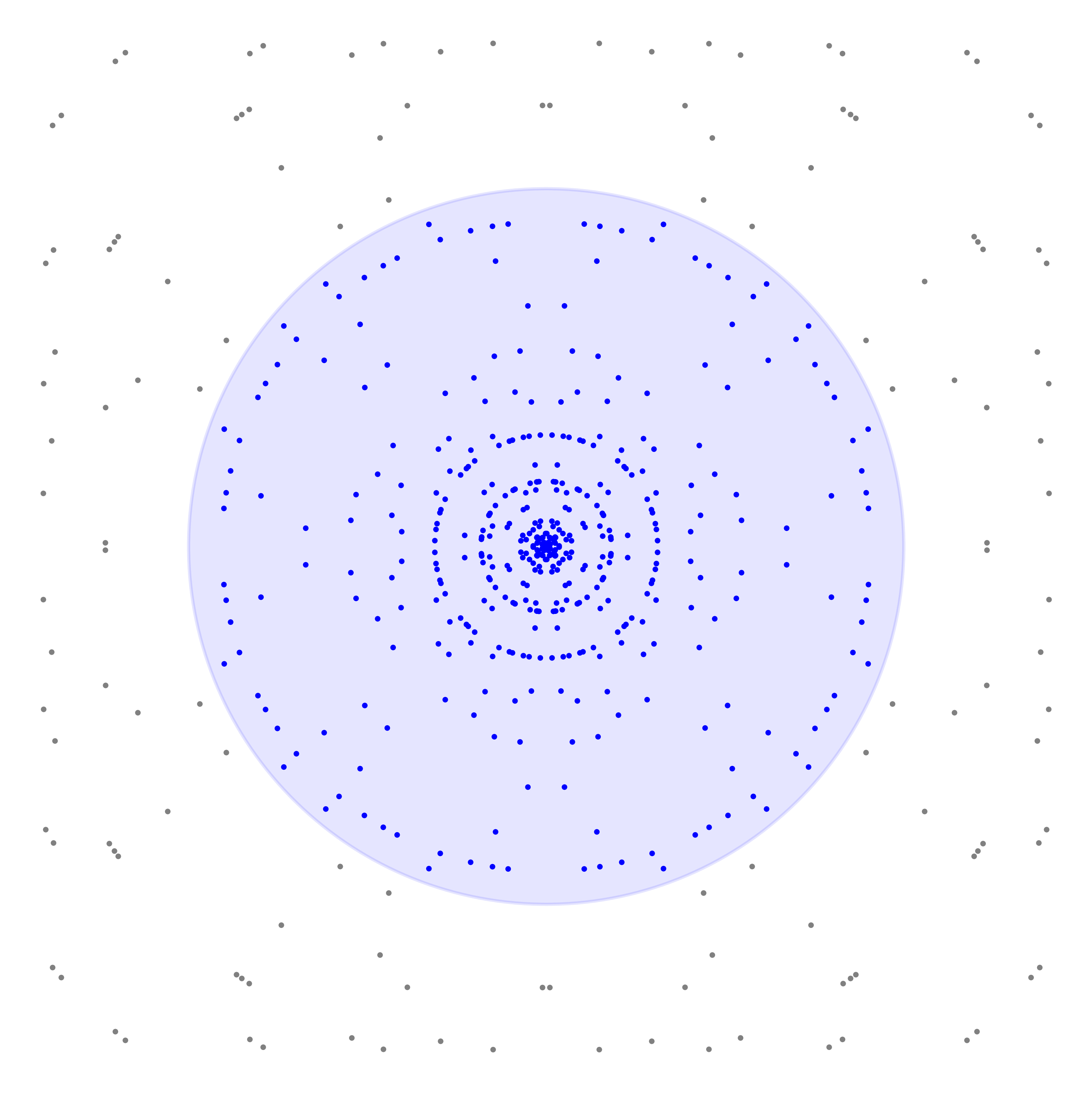
(a) $\Omega=\mathbb{D}\colonequals\mathopen{}\mathclose{{\left\{z\in\mathbb{C}:|z|\leq 1}}\right\}$.

(b) $\Omega=\mathopen{}\mathclose{{\left\{x+iy\in\mathbb{C}:\max(|x|,|y|)\leq 1}}\right\}$.

Figure 2. The lattice points plotted above correspond to Gaussian integers $\alpha$ such that the ideal $\mathfrak{a}=(\alpha)$ is twist minimal. The region $H\Omega$ is colored blue.

4.1. Setup

Let $\mathbb{Z}[i]$ denote the ring of Gaussian integers, with fraction field $\mathbb{Q}(i)$. Let $\mathcal{I}$ denote the multiplicative monoid of (nonzero) integral ideals in $\mathbb{Z}[i]$. For every $\mathfrak{a}=(\alpha)\in\mathcal{I}$, we denote by $N\mathfrak{a}\colonequals\#\mathopen{}\mathclose{{\left(\mathbb{Z}[i]/\mathfrak{a}}}\right)=\alpha\bar{\alpha}$ its norm. Let $\mathbb{D}\subset\mathbb{C}$ denote the closed unit ball.

Definition 4.1.

We say that a region $\Omega$ in $\mathbb{C}$ is squareish if it satisfies the following properties.

1. $0\in\Omega$.

2. $\Omega$ is compact.

3. There is a piecewise-smooth continuous function $\omega\colon\mathbb{R}\to\mathbb{R}_{\geq 0}$ of period $\pi/2$ such that

   $$\Omega=\mathopen{}\mathclose{{\left\{re^{i\theta}:r\in\mathbb{R},\theta\in[0,2\pi],\text{ and }0\leq r\leq\omega(\theta)}}\right\}.$$

Fix $s\in\mathbb{C}$, and consider the function $\omega(\theta)^{2s}$. This function admits a Fourier expansion of the form

(4.1) $$\omega(\theta)^{2s}\colonequals\sum_{k\in 4\mathbb{Z}}I_{\Omega,k}(s)e^{ik\theta},$$

where

(4.2) $$I_{\Omega,k}(s)=\frac{1}{2\pi}\int_{0}^{2\pi}\omega(\theta)^{2s}e^{-ik\theta}\,\mathrm{d}\theta=\frac{2}{\pi}\int_{0}^{\pi/2}\omega(\theta)^{2s}e^{-ik\theta}\,\mathrm{d}\theta.$$

Given $\mathfrak{a}\in\mathcal{I}$, let $\theta_{\mathfrak{a}}\in[0,\pi/2)$ be the argument of a generator $(\alpha)=\mathfrak{a}$ lying in the first quadrant. For every $k\in 4\mathbb{Z}$ we have the Hecke characters $\xi_{k}\colon\mathcal{I}\to\mathbb{C}^{\times}$ given by

(4.3) $$\xi_{k}(\mathfrak{a})\colonequals\mathopen{}\mathclose{{\left(\dfrac{\alpha}{|\alpha|}}}\right)^{ik}=e^{ik\theta_{\mathfrak{a}}},$$

where $\alpha$ is any generator of the ideal $\mathfrak{a}$. The final piece of data is a function $\phi\colon\mathcal{I}\to\mathbb{C}$ defined on ideals, and the corresponding twisted Dirichlet series

(4.4) $$L(s,\phi\otimes\xi_{k})\colonequals\sum_{\mathfrak{a}\in\mathcal{I}}\phi(\mathfrak{a})\xi_{k}(\mathfrak{a})(N\mathfrak{a})^{-s},\quad\text{ for }k\in 4\mathbb{Z}.$$

For our applications, $\phi$ is the characteristic function of some property, and an appropriate normalization of these Dirichlet series are $L$-functions (in the sense of [20, Section 5.1]). In particular, (4.4) converges absolutely in the half-plane $\mathrm{Re}(s)>\sigma_{0}>0$. When $k=0$, we abbreviate $L(s,\phi)\colonequals L(s,\phi\otimes\xi_{0})$. Note that when $\phi=\mathbf{1}$ is the constant function equal to one, $L(s,\mathbf{1})=\zeta_{K}(s)$ is the Dedekind zeta function of $K=\mathbb{Q}(i)$, and $L(s,\mathbf{1}\otimes\xi_{k})=L(s,\xi_{k})$ are the Hecke $L$-functions.

4.2. The main analytic lemma

Our goal is to understand the asymptotic main term in the counting function

(4.5) $$N_{\Omega}(H;\phi)\colonequals\sum_{\mathfrak{a}\in H\Omega}\phi(\mathfrak{a}),$$

where $H\Omega\colonequals\mathopen{}\mathclose{{\left\{Hz:z\in\Omega}}\right\}$. The abuse of notation $\mathfrak{a}\in H\Omega$ means that any generator $\alpha$ of $\mathfrak{a}$ is in the intersection $\mathbb{Z}[i]\cap H\Omega$. Since the norm is a quadratic function, we have that $\mathfrak{a}\in H\Omega$ if and only if $N\mathfrak{a}\leq\omega(\theta_{\mathfrak{a}})^{2}H^{2}$.

Lemma 4.2 (Main analytic lemma).

Suppose that $\Omega\subset\mathbb{Z}$ is a squareish region, and that $\phi\colon\mathcal{I}\to\mathbb{C}$ is a function satisfying the following:

1. $L(s,\phi)$ has reasonable analytic properties:

   1. $\phi(\mathfrak{a})\in\mathbb{R}_{>0}$ for all $\mathfrak{a}\in\mathcal{I}$.

   2. There exists some $\sigma_{0}\in\mathbb{R}_{>0}$ such that $L(s,\phi)$ converges absolutely in the half-plane $\mathrm{Re}(s)>\sigma_{0}>0$.

   3. $L(s,\phi)$ admits a meromorphic continuation to a half-plane $\mathrm{Re}(s)>\sigma_{0}-\delta_{0}>0$.

   4. In this domain, $L(s,\phi)$ has a unique pole. It is a simple pole of order $r=r(\phi)>0$, at $s=\sigma_{0}$. We denote

      $$\Theta(\phi)\colonequals\lim_{s\to\sigma_{0}}(s-\sigma_{0})^{r}L(s,\phi)>0.$$

   5. In the half-plane $\mathrm{Re}(s)>\sigma_{0}-\delta_{0}$, we have the convexity bound

      $$|L(s,\phi)(s-\sigma_{0})^{r}/s^{r}|=O(|1+\mathrm{Im}(s)|^{\kappa}),$$

      for some $\kappa=\kappa(\phi)>0$.

2. For every $0\neq k\in 4\mathbb{Z}$, there exist real valued functions $B_{\phi}(H,k)$ such that:

   • $B_{\phi}(H,k)=o(H^{2\sigma_{0}})$ as $H\to\infty$,

   • $B_{\phi}(H,k)=o(k^{m})$ as $k\to\infty$ for some positive $m>0$, and

   • we have the bound

     $$\mathopen{}\mathclose{{\left|\sum_{N\mathfrak{a}\leq H^{2}}\phi(\mathfrak{a})\xi_{k}(\mathfrak{a})}}\right|\leq B_{\phi}(H,k).$$

Then, there exists a monic polynomial $P(T)=P_{\phi,\Omega}(T)\in\mathbb{R}[T]$ of degree $r-1$ such that for every $0<\delta<\delta_{0}$, the asymptotic formula

$$N_{\Omega}(H;\phi)=\dfrac{I_{\Omega,0}(\sigma_{0})\Theta(\phi)2^{r-1}}{(r-1)!}H^{2\sigma_{0}}P(\log H)+O\mathopen{}\mathclose{{\left(\max\mathopen{}\mathclose{{\left\{\sum_{0\neq k\in 4\mathbb{Z}}\frac{B_{\phi}(H,k)}{k^{m+2}},H^{2(\sigma_{0}-\delta)}}}\right\}}}\right)$$

holds as $H\to\infty$. Here, the implicit constant depends on $\delta,\Omega$, and $\phi$.

Remembering the formula for area in terms of polar coordinates gives the following corollary.

Corollary 4.3.

In the situation of Lemma 4.2, if $\sigma_{0}=1$, then we have

$$N_{\Omega}(H;\phi)\sim\dfrac{\operatorname{vol}(\Omega)}{\pi}N_{\mathbb{D}}(H;\phi).$$

Proof of Lemma 4.2.

Let $c\colonequals\sigma_{0}+1$. From Perron’s integral, we have

(4.6) $$\dfrac{1}{2\pi i}\int_{c-i\infty}^{c+i\infty}\mathopen{}\mathclose{{\left(\dfrac{\omega(\theta_{\mathfrak{a}})^{2}H^{2}}{N\mathfrak{a}}}}\right)^{s}\dfrac{\,\mathrm{d}s}{s}=\begin{cases}1,&\text{ if }N\mathfrak{a}<\omega(\theta_{\mathfrak{a}})^{2}H^{2},\\ \tfrac{1}{2},&\text{ if }N\mathfrak{a}=\omega(\theta_{\mathfrak{a}})^{2}H^{2},\\ 0,&\text{ if }N\mathfrak{a}>\omega(\theta_{\mathfrak{a}})^{2}H^{2}.\end{cases}$$

for any fixed $\mathfrak{a}\in\mathcal{I}$. Replace $\omega(\theta)^{2s}$ by its Fourier expansion (4.1). The smoothness hypothesis implies the superpolynomial decay of $I_{\Omega,k}(s)$. This permits exchanging the order of integration and summation. Summing over all $\mathfrak{a}\in\mathcal{I}$ we obtain

(4.7) $$N_{\Omega}(H;\phi)=\dfrac{1}{2\pi i}\sum_{k\in 4\mathbb{Z}}\int_{c-i\infty}^{c+i\infty}L(s,\phi\otimes\xi_{k})I_{\Omega,k}(s)H^{2s}\dfrac{\,\mathrm{d}s}{s},$$

which holds for almost all $H>0$. In particular, $H$ can be chosen so that the Perron integral does not equal $\frac{1}{2}$ for all $\mathfrak{a}\in\mathcal{I}$.

The proof proceeds in two steps. First, we show that the dominant term in the sum is $k=0$ with negligible error

(4.8) $$N_{\Omega}(\phi;H)=\dfrac{1}{2\pi i}\int_{c-i\infty}^{c+i\infty}L(s,\phi)I_{\Omega,0}(s)H^{2s}\dfrac{\,\mathrm{d}s}{s}+O\mathopen{}\mathclose{{\left(\sum_{0\neq k\in 4\mathbb{Z}}\frac{B_{\phi}(H,k)}{k^{m+2}}}}\right),$$

for some positive integer $m$. Then, we show that

(4.9) $$\dfrac{1}{2\pi i}\int_{c-i\infty}^{c+i\infty}L(s,\phi)I_{\Omega,0}(s)H^{2s}\dfrac{\,\mathrm{d}s}{s}=\dfrac{I_{\Omega,0}(\sigma_{0})\Theta(\phi)2^{r-1}}{(r-1)!}H^{2\sigma_{0}}P(\log H)+O(H^{2(\sigma_{0}-\delta)}).$$

We will show these assertions in Lemma 4.4 and Lemma 4.5. When $\sigma_{0}=1$, the corollary follows from the area formula in polar coordinates:

$$\dfrac{\operatorname{vol}(\Omega)}{\operatorname{vol}(\mathbb{D})}=\frac{1}{\pi}\int_{0}^{2\pi}\frac{1}{2}\omega(\theta)^{2}\,\mathrm{d}\theta=I_{\Omega,0}(1).$$

∎

Lemma 4.4.

Assertion (4.8) holds.

Proof.

Let $c\colonequals\sigma_{0}+1$. Starting from Equation 4.7, we need to show that for some positive integer $m$,

$$\dfrac{1}{2\pi i}\sum_{0\neq k\in 4\mathbb{Z}}\int_{c-i\infty}^{c+i\infty}L(s,\phi\otimes\xi_{k})I_{\Omega,k}(s)H^{2s}\dfrac{\,\mathrm{d}s}{s}=O\mathopen{}\mathclose{{\left(\sum_{0\neq k\in 4\mathbb{Z}}\frac{B_{\phi}(H,k)}{k^{m+2}}}}\right).$$

For every individual $0\neq k\in 4\mathbb{Z}$, Item (ii) ensures that there exists a function $B_{\phi}(H,k)$, depending only on $\phi$, uniformly bounding the sums $\sum\phi(\mathfrak{a})\xi_{k}(\mathfrak{a})$. On the other hand, the superpolynomial decay of $I_{\Omega,k}(s)$ gives us a constant $C_{m}(\Omega)>0$, independent of $k$, such that $|I_{\Omega,k}(s)|\leq C_{m}(\Omega)|/|k|^{m}$ for every $m\in\mathbb{Z}_{>0}$. From the triangle inequality, we have that

$$\mathopen{}\mathclose{{\left|\dfrac{1}{2\pi i}\int_{c-i\infty}^{c+i\infty}L(s,\phi\otimes\xi_{k})I_{\Omega,k}(s)H^{2s}\dfrac{\,\mathrm{d}s}{s}}}\right| \leq\dfrac{C_{m}(\Omega)}{|k|^{m}}\mathopen{}\mathclose{{\left|\dfrac{1}{2\pi i}\int_{c-i\infty}^{c+i\infty}L(s,\phi\otimes\xi_{k})H^{2s}\dfrac{\,\mathrm{d}s}{s}}}\right|$$

$$\leq\dfrac{C_{m}(\Omega)}{|k|^{m}}\mathopen{}\mathclose{{\left|\sum_{N\mathfrak{a}\leq H^{2}}\phi(\mathfrak{a})\xi_{k}(\mathfrak{a})}}\right|\leq\dfrac{C_{m}(\Omega)}{|k|^{m}}B_{\phi}(H,k).$$

Taking $m$ sufficiently large, and summing over all $0\neq k\in 4\mathbb{Z}$, we obtain the result. ∎

Lemma 4.5.

Assertion (4.9) holds.

Proof.

Let $c\colonequals\sigma_{0}+1$. The idea is the standard trick of shifting the vertical segment from $-c-iT$ to $c+iT$ to the vertical segment from $\sigma_{0}-\delta-iT$ to $\sigma_{0}-\delta+iT$, for some $0<\delta<\delta_{0}$, so that we pick up the pole at $s=\sigma_{0}$. Then we can write the integral on the left hand side of Equation 4.9 as

(4.10) $$\operatorname{Res}_{s=\sigma_{0}}\mathopen{}\mathclose{{\left[L(s,\phi)I_{\Omega,0}(s)H^{2s}/s}}\right]+\frac{1}{2\pi i}\int_{\Gamma_{\delta,T}}L(s,\phi)I_{\Omega,0}(s)H^{2s}\frac{\,\mathrm{d}s}{s}.$$

Instead of repeating the proof of the Weiner–Ikehara Tauberian theorem (see for instance [10, Appendice A]), we explain how the extraneous factor $I(s)=I_{\Omega,0}(s)$ transforms the asymptotic.

Using the fact that $I(s)$ is uniformly bounded in the strip $\sigma_{0}-\delta\leq\mathrm{Re}(s)\leq c$, we see that

$$\frac{1}{2\pi i}\int_{\Gamma_{\delta,T}}L(s,\phi)I(s)H^{2s}\frac{\,\mathrm{d}s}{s}=O\mathopen{}\mathclose{{\left(\frac{1}{2\pi i}\int_{\Gamma_{\delta,T}}L(s,\phi)H^{2s}\frac{\,\mathrm{d}s}{s}}}\right).$$

Choosing an appropriate value of $T$ in terms of $H$, the proof of the classical theorem gives that this term is $O(H^{2(\sigma_{0}-\delta)})$.

To calculate the residue, we compute the Laurent expansions of the terms around $s=\sigma_{0}$ and calculate the coefficient of $(s-\sigma_{0})^{-1}$ in their product. We have:

$$L(s,\phi) =\sum_{n=-r}^{\infty}\Theta_{n}(s-\sigma_{0})^{n},$$

$$I(s) =\sum_{a=0}^{\infty}\tfrac{I^{(a)}(\sigma_{0})}{a!}(s-\sigma_{0})^{a},$$

$$H^{2s} =\sum_{b=0}^{\infty}\tfrac{H^{2\sigma_{0}}(2\log H)^{b}}{b!}(s-\sigma_{0})^{b},$$

$$1/s =\sum_{c=0}^{\infty}\tfrac{(-1)^{c}}{\sigma_{0}^{n+1}}(s-\sigma_{0})^{c},$$

It follows that the residue is given by the formula

(4.11) $$\operatorname{Res}_{s=\sigma_{0}}\mathopen{}\mathclose{{\left[L(s,\phi)I(s)H^{2s}/s}}\right]=\sum_{n+a+b+c=-1}\Theta_{n}\tfrac{I^{(a)}(1)}{a!}\tfrac{H^{2}2^{b}(\log H)^{b}}{b!}\tfrac{(-1)^{c}}{\sigma_{0}^{c+1}}.$$

In particular, the main term occurs when $n=-r$, $b=r-1$, and $a=c=0$, so that the leading constant in the asymptotic is

(4.12) $$I_{\Omega,0}(\sigma_{0})\cdot\dfrac{\Theta_{-r}2^{r-1}}{\sigma_{0}(r-1)!}>0.$$

∎

5. Proof of Theorem 1.1

We already know how to count minimal Fermat triples $(a,b,c)$ with $|c|\leq H$. We give a bijective correspondence between such triples and 5-isogenies $(E_{a,b,c},C_{a,b,c})$, up to isomorphism. Thus, we can write our counting function as

$$N_{5}(H)=\#\mathopen{}\mathclose{{\left\{(a,b,c)\in\mathscr{G}\langle\mathbb{Q}\rangle:\operatorname{Ht}(E_{a,b,c})\leq H}}\right\},$$

where $\operatorname{Ht}(E_{a,b,c})$ is the naive height of $E_{a,b,c}$ as in Equation 1.1. We have the compact region

(5.1) $$\mathcal{R}_{5}\colonequals\mathopen{}\mathclose{{\left\{(x,y)\in\mathbb{R}^{2}:H\mathopen{}\mathclose{{\left(x,y}}\right)\leq 1}}\right\}.$$

The strategy is to write $N_{5}(H)$ as a rescaling of $N_{\mathcal{R}_{5}}(H;\phi)$ for some arithmetic function $\phi$, and then use the main analytic lemma (Lemma 4.2) to complete the proof. To do this, we need to overcome two obstacles:

1. Firstly, the region $\mathcal{R}_{5}$ is not squareish. To overcome this, we partition $\mathcal{R}_{5}=\mathcal{R}_{5}^{(i)}\sqcup\mathcal{R}_{5}^{(ii)}\sqcup\mathcal{R}_{5}^{(iii)}\sqcup\mathcal{R}_{5}^{(iv)}$ into its quadrants, and rotate each component to obtain four squareish regions $\Omega^{(i)},\Omega^{(ii)},\Omega^{(iii)},\Omega^{(iv)}$. Further details can be found in Section 5.2.

2. Secondly, even when $(a,b,c)$ is a minimal triple, our chosen Weierstrass model for $E_{a,b,c}$ is not always a minimal one. We overcome this issue by carefully quantifying how far is $E_{a,b,c}$ from being minimal, and counting these finitely many degenerate cases separately. Further details can be found in Section 5.1 and Section 5.3.

5.1. The parametrization

Given a minimal Fermat triple $(a,b,c)$, consider the curve whose Weierstrass equation is given by

(5.2) $$\mathsf{y}^{2}=\mathsf{x}^{3}+A(a,b,c)\mathsf{x}+B(a,b,c),$$

where

(5.3) $$A(a,b,c) \colonequals-6(123a+114b+125c^{2})$$

$$=-(2\cdot 3^{2}\cdot 41)a-(2^{2}\cdot 3^{2}\cdot 19)b-(2\cdot 3\cdot 5^{3})c^{2},$$

(5.4) $$B(a,b,c) \colonequals 8c(2502a+261b+2500c^{2})$$

$$=(2^{4}\cdot 3^{2}\cdot 139)ac+(2^{3}\cdot 3^{2}\cdot 29)bc+(2^{5}\cdot 5^{4})c^{3}.$$

When the discriminant $\Delta(a,b,c)\colonequals-16(4A(a,b,c)^{3}+27B(a,b,c)^{2})$ is not zero, the smooth projective model of Equation 5.2 is an elliptic curve $E_{a,b,c}$ defined over $\mathbb{Q}$. Furthermore, this elliptic curve admits a rational $5$-isogeny $C_{a,b,c}\subseteq E_{a,b,c}(\bar{\mathbb{Q}})[5]$. Indeed, the $5$-division polynomial (see [31, Exercise 3.7]) $\psi_{5}(T;E_{a,b,c})\in\mathbb{Z}[a,b,c][T]$ has a quadratic factor

(5.5) $$h(a,b,c;T)\colonequals 5T^{2}-100cT-2106a-1750c^{2}+792b.$$

The cyclic group $C_{a,b,c}$ is defined as the group generated by the points $P\in E_{a,b,c}(\bar{\mathbb{Q}})[5]$ whose $\mathsf{x}$-coordinates are the roots of $h(a,b,c;T)$.

We will denote by $\mathscr{X}\langle\mathbb{Q}\rangle$ the set of isomorphism classes of the groupoid $\mathscr{X}(\mathbb{Q})$. We have $\mathscr{X}_{0}(5)\langle\mathbb{Q}\rangle=X_{0}(5)(\mathbb{Q})$. As a corollary of Lemma 2.8 we have the following parametrization of isomorphism classes of $5$-isogenies in terms of minimal Fermat triples. Given a 5-isogeny $(E,C)$, we denote its $\mathbb{Q}$-isomorphism class by $[E,C]$.

Lemma 5.1.

The equivalence of Lemma 2.8 induces a bijection $\Phi\colon\mathscr{G}\langle\mathbb{Q}\rangle\to X_{0}(5)(\mathbb{Q})$. Under this map, the cusps $\Phi(Q_{1}),\Phi(Q_{2})\in X_{0}(5)(\mathbb{Q})$ correspond to the minimal triples

$$Q_{1}\colonequals(-1,0,1),\quad Q_{2}\colonequals(-528,220,25).$$

In particular, $\Phi$ restricts to an isomorphism

(5.6) $$\Phi\colon\mathscr{G}\langle\mathbb{Q}\rangle-\mathopen{}\mathclose{{\left\{Q_{1},Q_{2}}}\right\}\longrightarrow Y_{0}(5)(\mathbb{Q}),\quad(a,b,c)\mapsto[E_{a,b,c},C_{a,b,c}].$$

The identical parametrization of twist minimal isomorphism classes of $5$-isogenies in terms of twist minimal Fermat triples also holds. Given a $5$-isogeny $(E,C)$ defined over $\mathbb{Q}$, we denote its $\bar{\mathbb{Q}}$-isomorphism class by $\langle E,C\rangle$.

Lemma 5.2.

The equivalence of Lemma 2.8 induces a bijection $\Psi\colon\mathscr{F}\langle\mathbb{Q}\rangle\to\mathscr{Z}_{0}(5)\langle\mathbb{Q}\rangle$. Likewise, the cusps $\Psi(Q_{1}),\Psi(Q_{2})\in\mathscr{Z}_{0}(5)(\mathbb{Q})$ correspond to the twist minimal Fermat triples

$$Q_{1}\colonequals(-1,0,1),\quad Q_{2}\colonequals(-528,220,25).$$

In particular, $\Psi$ restricts to an isomorphism

(5.7) $$\Psi\colon\mathscr{F}\langle\mathbb{Q}\rangle-\mathopen{}\mathclose{{\left\{Q_{1},Q_{2}}}\right\}\longrightarrow(\mathscr{Z}_{0}(5)\langle\mathbb{Q}\rangle-\mathopen{}\mathclose{{\left\{\Psi(Q_{1}),\Psi(Q_{2})}}\right\}),\quad(a,b,c)\mapsto\langle E_{a,b,c},C_{a,b,c}\rangle.$$

Observe that the representatives $(E_{a,b,c},C_{a,b,c})$ of the isomorphism classes in Lemma 5.1 and Lemma 5.2 do not need to correspond to a minimal Weierstrass equation.

Definition 5.3.

A Weierstrass equation of the elliptic curve $E\colon\mathsf{y}^{2}=\mathsf{x}^{3}+A\mathsf{x}+B$ is twist minimal if no prime $p$ satisfies $p^{2}\mid A$ and $p^{3}\mid B$.

Since the naive height (1.1) is calculated from the coefficients of a minimal model, it is necessary to understand the twist minimal triples $(a,b,c)$ giving rise to Weierstrass equations $E_{a,b,c}$ that are not twist minimal.

Definition 5.4.

The twist minimality defect of a Fermat triple $(a,b,c)$, denoted by $\operatorname{tmd}(E_{a,b,c})$, is

$$\operatorname{tmd}(E_{a,b,c})\colonequals\max\{e\in\mathbb{Z}_{>0}\;:\;e^{2}\mid A(a,b,c)\text{ and }e^{3}\mid B(a,b,c)\}.$$

In the notation of [26], this is precisely the twist minimality defect of the Weierstrass equation $E_{a,b,c}$. We say that a twist minimal Fermat triple $(a,b,c)$ is exceptional if $\operatorname{tmd}(E_{a,b,c})>1$.

We classify the exceptional twist minimal Fermat triples.

Proposition 5.5.

Let $(a,b,c)$ be a twist minimal Fermat triple.

1. The set of all possible values of $\operatorname{tmd}(E_{a,b,c})$ is

   $$\mathsf{TMD}\colonequals\{1,2,5,10,25,50,125,250\}.$$

2. $2\mid\operatorname{tmd}(E_{a,b,c})$ if and only if $2\mid b$. Moreover, the $2$-adic valuations of $A(a,b,c),B(a,b,c),$ and $\operatorname{tmd}(E_{a,b,c})$ can be found in Table 2.

3. $5\mid\operatorname{tmd}(E_{a,b,c})$ if and only if $\alpha=a+ib$ for any one of $\alpha\in\mathbb{Z}[i]$ provided in Table 3.

$\operatorname{ord}_{2}(A)$	$\operatorname{ord}_{2}(B)$	$\operatorname{ord}_{2}(\operatorname{tmd})$
$1$	$3$	$0$
$\geq 2$	$4$	$1$

Table 2. $2$-adic valuations of $A(a,b,c)$, $B(a,b,c)$, and $\operatorname{tmd}(E_{a,b,c})$.

$\alpha=a+ib\in\mathbb{Z}[i]$	$\operatorname{ord}_{5}(A)$	$\operatorname{ord}_{5}(B)$	$\operatorname{ord}_{5}(\operatorname{tmd})$
$(1-2i)^{4}\beta$	$4$	$5$	$1$
$5(1-2i)^{2}\beta$	$3$	$4$	$1$
$(1-2i)^{4k}\beta$, $k\geq 2$	$5$	$k+7$	$2$
$5(1-2i)^{6}\beta$	$6$	$9$	$3$
$5(1-2i)^{4k-2}\beta$, $k\geq 3$	$6$	$k+8$	$3$

Table 3. $5$-adic valuations of $A(a,b,c)$, $B(a,b,c)$, and $\operatorname{tmd}(E_{a,b,c})$. Here, $\beta\in\mathbb{Z}[i]$ is any element of norm coprime to $5$.

Proof.

We break up the proof of the proposition into a number of lemmas in modular arithmetic. All the Fermat triples below are assumed to be twist minimal.

The first two statements follow by combining the statements of Lemmas 5.8, 5.9, 5.10, and 5.11. The last statement follows from Lemma 5.12. ∎

Lemma 5.6.

If a prime $p$ satisfies $p\mid c$ and $p^{2}\mid A(a,b,c),$ then $p=5$.

Proof.

From Lemma 3.5, every prime $p$ dividing $c$ satisfies $p\equiv 1\text{ mod }4$. Thus, $p\neq 2,3$. Assume that $p\neq 5$. Reducing Equation 5.3 modulo $p^{2}$ gives $123a\equiv-114b\text{ mod }p^{2}$. This implies that

$$(123c^{2})^{2} =(123a)^{2}+(123b)^{2}$$

$$\equiv(-114b)^{2}+(123b)^{2}\text{ mod }p^{2}$$

$$\equiv(114^{2}+123^{2})b^{2}\text{ mod }p^{2}\equiv 3^{2}\cdot 5^{5}\cdot b^{2}\equiv 0\text{ mod }p^{2}.$$

It follows that $p\mid b$, and therefore $p\mid a$ as well. Let $a^{\prime}\colonequals a/p$, $b^{\prime}\colonequals b/p$ and $c^{\prime}\colonequals c/p$. We have that $(a^{\prime})^{2}+(b^{\prime})^{2}=p^{2}(c^{\prime})^{4}$ and $123a^{\prime}+114b^{\prime}+125p(c^{\prime})^{2}\equiv 0\text{ mod }p$. Once more, it follows that $123a^{\prime}\equiv-114b^{\prime}\text{ mod }p$, and

$$(123a^{\prime})^{2}+(123b^{\prime})^{2} \equiv(114^{2}+123^{2})(b^{\prime})^{2}\text{ mod }p$$

$$\equiv 3^{2}\cdot 5^{5}\cdot(b^{\prime})^{2}\equiv 0\text{ mod }p.$$

This allows us to conclude that $p\mid b^{\prime}$, and therefore $p\mid a^{\prime}$ as well. This contradicts the twist minimality of the triple $(a,b,c)$.

To see that the case $p=5$ indeed occurs, one can take $(a,b,c)=(-527,-336,25)$. This triple is twist minimal, since $\gcd(a,b)=1$, and $A(a,b,c)=2^{4}\cdot 3\cdot 5^{5}$. ∎

Lemma 5.7.

If $p$ is a prime divisor of $\operatorname{tmd}(E_{a,b,c})$, then $p\in\mathopen{}\mathclose{{\left\{2,5}}\right\}$.

Proof.

By definition, $p\mid\operatorname{tmd}(E_{a,b,c})$ if and only if $p^{2}\mid A\colonequals A(a,b,c)$ and $p^{3}\mid B\colonequals B(a,b,c)$. If $p$ also divided $c$, then Lemma 5.6 implies that $p=5$. For this reason, we assume that $p$ does not divide $c$.

We use the equations $A\equiv 0\text{ mod }p^{2}$ and $B\equiv 0\text{ mod }p^{2}$ to find congruence relations between $a$ and $b$ modulo $p^{2}$. We find integer linear combinations of $cA$ and $B$ that allow us to cancel the terms with $a$ or $b$ in them, obtaining:

$$1112cA+41B =-(14000c^{3}+675000bc)=-2^{3}5^{3}c(14c^{2}+675b)\equiv 0\text{ mod }p^{2},$$

$$58ca+19B =337500ac+336500c^{3}=2^{2}5^{3}c(673c^{2}+675a)\equiv 0\text{ mod }p^{2}.$$

If $p\neq\mathopen{}\mathclose{{\left\{2,5}}\right\}$, then $(14c^{2}+675b)\equiv 0\text{ mod }p^{2}$ and $(673c^{2}+675a)\equiv 0\text{ mod }p^{2}$. But in this case, we can reduce the equation $(675a)^{2}+(675b)^{2}=675^{2}c^{4}$ modulo $p^{2}$ to obtain

$$5^{6}\cdot 29=14^{2}+673^{2}\equiv 675^{2}=3^{6}\cdot 5^{4}\text{ mod }p^{2},$$

producing a contradiction. We conclude that in this case $p\in\mathopen{}\mathclose{{\left\{2,5}}\right\}$, and the result follows. ∎

Lemma 5.8.

The following assertions hold.

1. $2\mid\operatorname{tmd}(E_{a,b,c})$ if and only if $2\mid b$.

2. $5\mid\operatorname{tmd}(E_{a,b,c})$ if and only if $a\equiv 7b\text{ mod }25$ and $5\mid c$.

We say that $(a,b,c)$ is 2-exceptional when (a) holds, and 5-exceptional when (b) holds.

Proof.

1. If $2\mid\operatorname{tmd}(E_{a,b,c})$, then $4\mid A$. This implies that $a$ and $c$ have the same parity. Since $c\equiv 1\text{ mod }4$, $a$ must be odd. But since $a$ and $b$ have opposite parity, we conclude that $2\mid b$. Conversely, suppose that $2\mid b$. This implies that $a$ is odd. Since $8\mid B$, we only need to show that $4\mid A$. But this is visibly true once we know that $a$ is odd.

2. If $5\mid\operatorname{tmd}(E_{a,b,c})$, then $A\equiv 0\text{ mod }25$. This implies that $a\equiv 7b\text{ mod }25$. From this congruence, we see that $c^{4}=a^{2}+b^{2}=50b^{2}\equiv 0\text{ mod }25$, so that $5\mid c$. Conversely, the congruence $a\equiv 7b\text{ mod }25$ implies that $A\equiv 0\text{ mod }25$ and $B/(8c)\equiv 0\text{ mod }25$, which is enough to conclude that $5\mid\operatorname{tmd}(E_{a,b,c})$.

∎

Lemma 5.9.

The quantity $\operatorname{tmd}(E_{a,b,c})$ is not divisible by $4$.

Proof.

Suppose that $4\mid\operatorname{tmd}(E_{a,b,c})$. By definition, this means that $4^{2}\mid A$ and $4^{3}\mid B$. From Equations 5.3 and 5.4, we deduce that

$$123a+114b+125c^{2} \equiv 0\text{ mod }8,$$

$$2502a+261b+2500c^{2} \equiv 0\text{ mod }8.$$

Since $c\equiv 1\text{ mod }4$ (Lemma 3.5), we have that $c^{2}\equiv 1\text{ mod }8$, and the above congruences simplify to:

$$3a+2b+5 \equiv 0\text{ mod }8,$$

$$6a+5b+4 \equiv 0\text{ mod }8.$$

These imply that $b\equiv 6\text{ mod }8$, and $a^{2}+b^{2}=c^{4}$ implies that $a^{2}\equiv 5\text{ mod }8$. But this contradicts the fact that $5$ is not a square modulo $8$. ∎

Lemma 5.10.

If $\operatorname{tmd}(E_{a,b,c})$ is divisible by $2$, then $\operatorname{ord}_{2}(A(a,b,c))\geq 2$ and $\operatorname{ord}_{2}(B(a,b,c))=4$. Otherwise, $\operatorname{ord}_{2}(A(a,b,c))=1$ and $\operatorname{ord}_{2}(B(a,b,c))=3$.

Proof.

Suppose $2\mid\operatorname{tmd}(E_{a,b,c})$. Using $a^{2}+b^{2}=c^{4}$ mod $16$, one obtains that $4\mid b$, $a\equiv 1,7,9,15\text{ mod }16$, and $c^{2}\equiv 1,9\text{ mod }16$. It follows that $\text{ord}_{2}(A(a,b,c))\geq 2$ and $\operatorname{ord}_{2}(B(a,b,c))=4$. The case for $2\nmid\operatorname{tmd}(E_{a,b,c})$ follows from the fact that $b$ and $c$ are odd. ∎

Lemma 5.11.

The quantity $\operatorname{tmd}(E_{a,b,c})$ is not divisible by $5^{4}$.

Proof.

Suppose that $5^{4}\mid\operatorname{tmd}(E_{a,b,c})$. By definition, this implies that $5^{8}\mid A$ and $5^{12}\mid B$. Using Equations 5.3 and 5.4, we deduce that

$$123a+114b+125c^{2} \equiv 0\text{ mod }5^{8}$$

$$c(2502a+261b+2500c^{2}) \equiv 0\text{ mod }5^{12}.$$

We consider four cases depending on the 5-valuation of $c$.

Case 1: Suppose $\operatorname{ord}_{5}(c)\geq 3$. Then, $41a+38b\equiv 0\text{ mod }5^{8}$. This congruence simplifies to $a\equiv 323932b\text{ mod }5^{8}$. Using the equation $a^{2}+b^{2}=c^{4}$, we obtain

$$a^{2}+b^{2}\equiv 300000a^{2}=2^{5}\cdot 3\cdot 5^{5}a^{2}\equiv 0\text{ mod }5^{8}.$$

This implies that $a\equiv b\equiv 0\text{ mod }5^{2}$, contradicting the twist minimality of $(a,b,c)$.

Case 2: Suppose that $\operatorname{ord}_{5}(c)=2$. We obtain the linear system

$$41a+38b \equiv 0\text{ mod }5^{7},$$

$$278a+29b \equiv 0\text{ mod }5^{7}.$$

Solving for $b$ in the first equation and substituting into the second one, we arrive at

$$18750a=2\cdot 3\cdot 5^{5}a\equiv 0\text{ mod }5^{7}.$$

This implies that $a\equiv b\equiv 0\text{ mod }5^{2}$, contradicting the twist minimality of $(a,b,c)$.

Case 3: Suppose that $\operatorname{ord}_{5}(c)=1$. Then $41a+38b\equiv 0\text{ mod }5^{5}$. Solving for $b$ we obtain $b\equiv 1068a\text{ mod }5^{5}$, which implies

$$a^{2}+b^{2}\equiv 3125a^{2}\equiv 5^{5}a^{2}\equiv 0\equiv c^{4}\text{ mod }5^{5}.$$

This implies that $5^{2}\mid c$, a contradiction.

Case 4: Suppose that $\operatorname{ord}_{5}(c)=0$. Then Equation 5.4 implies $278a+29b\equiv 0\text{ mod }5^{4}$. Solving for $b$, we obtain $b\equiv 497\text{ mod }5^{4}$, which implies

$$c^{4}=a^{2}+b^{2}\equiv 625a^{2}\equiv 5^{4}a^{2}\equiv 0\text{ mod }5^{4}.$$

This implies that $5\mid c$, a contradiction. ∎

Lemma 5.12.

Let $(a,b,c)$ be a $5$-exceptional triple, and let $\alpha=a+bi\in\mathbb{Z}[i]$. Then, we can write $\alpha=\delta\cdot\beta$ where $\beta$ and $\delta$ are coprime twist minimal Gaussian integers, and $\delta$ is given as in Table 4.

$\operatorname{ord}_{5}(\operatorname{tmd}(E_{a,b,c}))$	$\delta$	$k$
$1$	$(1-2i)^{4}$	-
$1$	$5(1-2i)^{2}$	-
$2$	$(1-2i)^{4k}$	$\geq 2$
$3$	$5(1-2i)^{4k-2}$	$\geq 2$

Table 4. Gaussian factors of $5$-exceptional triples.

Proof.

Since $(a,b,c)$ is $5$-exceptional, we know that $\operatorname{ord}_{5}(c)=k\geq 1$. Moreover, we can write $\alpha=\delta\cdot\beta$ so that $\beta$ is coprime to both $1\pm 2i$. This implies that $\delta\in\mathopen{}\mathclose{{\left\{(1\pm 2i)^{4k},5(1\pm 2i)^{4k-2}}}\right\}$. On the other hand, observe that

(5.8) $$(1+2i)^{5}\alpha =(41-38i)(a+bi)=(41a+38b)+i(41b-38a),$$

(5.9) $$(1+2i)^{7}\alpha =(29+278i)(a+bi)=(29a-278b)+i(278a+29b).$$

Taking the norm and comparing the parity of $\operatorname{ord}_{5}(\cdot)$ on the two sides of the equation, we deduce that

$$\operatorname{ord}_{5}(41a+38b) =\operatorname{ord}_{5}(41b-38a)=\operatorname{ord}_{5}((1+2i)^{5}\alpha),$$

$$\operatorname{ord}_{5}(278a+29b) =\operatorname{ord}_{5}(29a-278b)=\operatorname{ord}_{5}((1+2i)^{7}\alpha).$$

Furthermore, since $5$ divides $A$ and $B$, we must have that $\delta\in\mathopen{}\mathclose{{\left\{(1-2i)^{4k},5(1-2i)^{4k-2}}}\right\}$. Taking $\operatorname{ord}_{5}(\cdot)$ on Equations 5.3 and 5.4 we obtain

(5.10) $$\operatorname{ord}_{5}(A(a,b,c)) \geq\min\mathopen{}\mathclose{{\left\{\operatorname{ord}_{5}((1+2i)^{5}\delta),3+2k}}\right\},$$

(5.11) $$\operatorname{ord}_{5}(B(a,b,c)) \geq k+\min\mathopen{}\mathclose{{\left\{\operatorname{ord}_{5}((1+2i)^{7}\delta),4+2k}}\right\},$$

with equality when the entries of the minimum functions are distinct. ∎

5.2. The rigidified count

We adopt the strategy of the proof of Theorem 3.2 and apply the main analytic lemma (Lemma 4.2) to obtain an explicit asymptotic formula for the counting functions

$$N_{5}^{\operatorname{tw}}(H,t)\colonequals\#\{(a,b,c)\in\mathscr{F}\langle\mathbb{Q}\rangle:\operatorname{tmd}(E_{a,b,c})=t,\,\operatorname{twHt}(E_{a,b,c})\leq H\}.$$

Observe that we are counting elliptic curves up to quadratic twists. Explicitly, our height function is

$$\operatorname{twHt}(E_{a,b,c})\colonequals\dfrac{\max\mathopen{}\mathclose{{\left\{4|A(a,b,c)|^{3},27B(a,b,c)^{2}}}\right\}}{\operatorname{tmd}(E_{a,b,c})^{6}}.$$

Theorem 5.13.

For each $t\in\mathsf{TMD}\colonequals\mathopen{}\mathclose{{\left\{1,2,5,10,25,50,125,250}}\right\}$, there exist explicitly computable constants $\hat{C}_{5,t},\hat{C^{\prime}}_{5,t}\in\mathbb{R}$ and a number $c\in(0,1)$ such that

$$N_{5}^{\operatorname{tw}}(H,t)=\hat{C}_{5,t}H^{1/6}(\log H)+\hat{C^{\prime}}_{5,t}H^{1/6}+O(H^{1/6}\cdot(\log H)^{-1+c})$$

as $H\to\infty$. The constants $\hat{C}_{5,t}$ are given by:

$$\hat{C}_{5,t}\colonequals\frac{f_{1}}{\pi}V_{5}\cdot\begin{cases}\frac{t}{128},&\text{ if }t\in\{1,2\},\\ \frac{t}{240},&\text{ if }t\in\{5,10\},\\ \frac{t}{1920},&\text{ if }t\in\{25,50,125,250\},\end{cases}$$

where $f_{1}$ is the constant defined in Theorem 3.4, and $V_{5}$ is an explicit constant given by Equation 5.17.

Given $t\in\mathsf{TMD}$, we define the twist minimality defect height zeta function corresponding to $N_{5}^{\operatorname{tw}}(H,t)$ to be the Dirichlet series

(5.12) $$F_{t}(s)\colonequals\sum_{c=1}^{\infty}\frac{f_{t}(c)}{c^{s}},$$

where we denote by $f_{t}(c)$ the twist minimality defect arithmetic height function that counts the number of twist minimal triples $(a^{\prime},b^{\prime},c^{\prime})$ with $c^{\prime}=c$ and $\operatorname{tmd}(a^{\prime},b^{\prime},c^{\prime})=t$. The following lemma is an analogue of Lemma 3.6.

Lemma 5.14.

The arithmetic height function $f_{t}(c)$ satisfies the following properties.

1. If $p\not\equiv 1\text{ mod }4$, then $f_{t}(p^{k})=0$ for every positive integer $k$.

2. Suppose $t\in\{1,2\}$.

   • If $p\equiv 1\text{ mod }4$ and $p\neq 5$, then $f_{t}(p^{k})=8$ for every positive integer $k$.

   • If $p=5$, then $f_{t}(5^{k})=4$ for every positive integer $k$.

   • The arithmetic function $f_{t}(c)/2$ is multiplicative, but not completely multiplicative.

3. Suppose $t\in\{5,10\}$.

   • Given any integer $c$, if $\operatorname{ord}_{5}(c)\neq 1$ then $f_{t}(c)=0$.

   • We have $f_{t}(5)=4$ and $f_{t}(5^{k})=0$ for every positive integer $k\geq 2$.

   • For any $c$ corpime to $5$, we have $f_{t}(5c)=4f_{\frac{t}{5}}(c).$

4. Suppose $t\in\{25,50,125,250\}$.

   • Given any integer $c$, if $\operatorname{ord}_{5}(c)\leq 1$, then $f_{t}(c)=0$.

   • We have $f_{t}(5)=0$, and $f_{t}(5^{k})=2$ for every positive integer $k\geq 2$.

   • For any $c$ coprime to $5$ and $k\geq 2$, we have $f_{t}(5^{k}c)=2f_{\frac{t}{25}}(c)$ if $t\in\{25,50\}$, and $f_{t}(5^{k}c)=2f_{\frac{t}{125}}(c)$ if $t\in\{125,250\}$.

Proof.

We recall from Lemma 5.8 that $2\mid\operatorname{tmd}(E_{a,b,c})$ if and only if $b$ is even. Because $(a,b,c)$ is twist minimal, $c$ is odd. This implies that one of $a$ and $b$ must be even. Without loss of generality, assume $b$ is even. Multiplication by $\pm i$ flips the role of $a$ and $b$. Statements (1) and (2) (except for the case where $p=5$) follow from adapting the technique of the proof shown in Lemma 3.6, in particular by using multiplicativity of the ideal norm. To check the statement for $p=5$, we use Lemma 5.12. Suppose that $\mathfrak{a}\subset\mathbb{Z}[i]$ is an ideal such that $5\nmid\operatorname{tmd}(E_{a,b,c})$ and $N\mathfrak{a}=5^{4k}$. There are two such ideals, namely the ones generated by $(1+2i)^{4k}$ and $5(1+2i)^{4k-2}$.

To check statements (3) and (4), we also use Lemma 5.12. If $\operatorname{tmd}(E_{a,b,c})=5$ or $10$, then there are only two such ideals $\mathfrak{a}\subset\mathbb{Z}[i]$, generated by $(1-2i)^{4}$ and $5(1-2i)^{2}$: both ideals have norm $N\mathfrak{a}=5^{4}$. If $\operatorname{tmd}(E_{a,b,c})=25$ or $50$, then for each $k\geq 2$ such that $N\mathfrak{a}=5^{4k}$, there is only one ideal $\mathfrak{a}\subset\mathbb{Z}[i]$ satisfying the aforementioned conditions: it is the ideal generated by $(1-2i)^{4k}$. Lastly, if $\operatorname{tmd}(E_{a,b,c})=125$ or $250$, then for each $k\geq 2$ such that $N\mathfrak{a}=5^{4k}$, there is only one ideal $\mathfrak{a}\subset\mathbb{Z}[i]$ satisfying the aforementioned conditions: it is the ideal generated by $5(1-2i)^{4k-2}$. To relate the arithmetic functions $f_{t}$ with $f_{\frac{t}{25}}$ or $f_{\frac{t}{125}}$, we use the fact that any ideal $\mathfrak{a}$ such that $5\mid\operatorname{tmd}(E_{a,b,c})$ must be of form $\delta\cdot\beta$ where $\delta$ has norm divisible by $5$, and $\beta$ is coprime to $5$. ∎

To prove Theorem 5.13, we check whether the two conditions of the main analytic lemma are satisfied. Given a squareish region $\Omega\subset\mathbb{C}$ and $t\in\mathsf{TMD}$, we define $\psi_{t}:\mathcal{I}\to\mathbb{C}$ to be the indicator function of those ideals $\mathfrak{a}=(\alpha)$ giving rise to a twist minimal triple $(a,b,c)$ with $\operatorname{tmd}(E_{a,b,c})=t$. We denote by

(5.13) $$L(\psi_{t},s)\colonequals\sum_{\mathfrak{a}\in\mathcal{I}}\psi_{t}(\mathfrak{a})(N\mathfrak{a})^{-s}$$

the corresponding Dirichlet series, as in Section 4.1. Recall the definition of $L(\psi,s)$ in Equation 3.8.

Lemma 5.15.

The Dirichlet series $L(\psi_{t},s)$ satisfy the reasonable analytic properties in Item (i) of Lemma 4.2, with $\sigma_{0}=\frac{1}{4}$, $\delta_{0}=\frac{1}{8}$, and $r=2$. Moreover, we have

$$L(\psi_{t},s)=\begin{cases}\mathopen{}\mathclose{{\left(\frac{1+5^{-4s}}{1+3\cdot 5^{-4s}}}}\right)L(\psi,s),&\quad\text{ if }t\in\mathopen{}\mathclose{{\left\{1,2}}\right\},\\ \frac{4}{5^{4s}}\mathopen{}\mathclose{{\left(\frac{1-5^{-4s}}{1+3\cdot 5^{-4s}}}}\right)L(\psi,s),&\quad\text{ if }t\in\mathopen{}\mathclose{{\left\{5,10}}\right\},\\ 2\mathopen{}\mathclose{{\left(\frac{5^{-8s}}{1+3\cdot 5^{-4s}}}}\right)L(\psi,s),&\quad\text{ if }t\in\{25,50,125,250\}.\end{cases}$$

Proof.

Suppose $t\in\{1,2\}$. From Lemma 3.6 and Lemma 5.14, we have that $f(c)=2f_{t}(c)$ as long as $c$ is coprime to $5$. This implies that for any $t\in\{1,2\}$, the height zeta functions $F_{t}(s)$ satisfy:

$$F_{t}(s)=\frac{1}{2}\mathopen{}\mathclose{{\left(\frac{1+5^{-s}}{1+3\cdot 5^{-s}}}}\right)F(s).$$

Now suppose that $t\in\{5,10\}$. Then we have

$$F_{t}(s) =\sum_{c=1}^{\infty}\frac{f_{t}(c)}{c^{s}}$$

$$=\sum_{\begin{subarray}{c}c=1\\ \operatorname{ord}_{5}(c)=1\end{subarray}}^{\infty}\frac{4f_{\frac{t}{5}}(\frac{c}{5})}{c^{s}}=\frac{4}{5^{s}}\sum_{\begin{subarray}{c}m=1\\ 5\,\nmid\,m\end{subarray}}^{\infty}\frac{f_{\frac{t}{5}}(m)}{m^{s}}=\frac{2}{5^{s}}\mathopen{}\mathclose{{\left(\frac{1-5^{-s}}{1+3\cdot 5^{-s}}}}\right)F(s).$$

Lastly, suppose that $t\in\{25,50,125,250\}$. Let $\nu$ momentarily denote the $5$-adic valuation $\operatorname{ord}_{5}$. Then we have

$$\begin{split}F_{t}(s)&=\sum_{c=1}^{\infty}\frac{f_{t}(c)}{c^{s}}=\sum_{k=2}^{\infty}\sum_{\begin{subarray}{c}c=1\\ \nu(c)=k\end{subarray}}^{\infty}\frac{2f_{\frac{t}{5^{\nu(t)}}}(\frac{c}{5^{k}})}{c^{s}}=\sum_{k=2}^{\infty}\frac{2}{5^{ks}}\sum_{\begin{subarray}{c}m=1\\ 5\,\nmid\,m\end{subarray}}\frac{f_{\frac{t}{5^{\nu(t)}}}(m)}{m^{s}}\\ &=\sum_{k=2}^{\infty}\frac{2}{5^{ks}}\cdot\frac{1}{2}F(s)\cdot\frac{1-5^{-s}}{1+3\cdot 5^{-s}}=\mathopen{}\mathclose{{\left(\frac{5^{-2s}}{1+3\cdot 5^{-s}}}}\right)F(s).\end{split}$$

Hence, the analytic properties of $F_{t}(s)$ are identical to those of $F(s)$, which are obtained in the proof of Theorem 3.4. The result follows from the identities (3.10) and

(5.14) $$L(\psi_{t},s)=\tfrac{1}{2}F_{t}(4s).$$

∎

Lemma 5.16.

For all $t\in\mathsf{TMD}$, the Dirichlet series $L(\psi_{t},s)$ satisfy the hypothesis Item (ii) of Lemma 4.2 with

$$B_{\psi_{t}}(H,k)\colonequals\frac{H^{1/2}}{(\log H)^{1-c}}\cdot\log k,$$

where $c=\frac{3\sqrt{3}}{4\pi}\in(0,1)$.

Proof.

The lemma follows from adapting the proof of angular equidstribution of Gaussian integers, as demonstrated in [16, Section 2]. Without loss of generality, we assume that $t=1$, and abbreviate $\psi_{1}=\psi$. The cases for other values of $t$ follow analogously, for some $c\in(0,\frac{3\sqrt{3}}{4\pi}]$.

Given an ideal $\mathfrak{a}\in\mathcal{I}$, denote by $\overline{\mathfrak{a}}$ its complex conjugate. Given a prime $p\equiv 1\text{ mod }4$, we denote by $\theta_{p}$ the argument of a generator of the prime ideal of norm $p$ lying in the first octant. Since $\theta_{\mathfrak{a}}=\frac{\pi}{2}-\theta_{\overline{\mathfrak{a}}}$ and $\psi(\mathfrak{a})=\psi(\overline{\mathfrak{a}})$, one can check that if $N\mathfrak{a}=p^{\ell}$ for some prime $p\equiv 1\text{ mod }4$ and a positive integer $\ell$, then

$$\psi(\mathfrak{a})\xi_{k}(\mathfrak{a})+\psi(\overline{\mathfrak{a}})\xi_{k}(\overline{\mathfrak{a}})=\begin{cases}2\psi(\mathfrak{a})\cos(k\ell\theta_{p}),&\text{ if }p\nmid\mathfrak{a},\\ 2\psi(\mathfrak{a})\cos(k(\ell-2)\theta_{p}),&\text{ if }p\parallel\mathfrak{a},\\ 0,&\text{ otherwise }.\end{cases}$$

Hence, we have for each $p$ and $k$,

$$\sum_{\begin{subarray}{c}\mathfrak{a}\in\mathcal{I}\\ N\mathfrak{a}=p^{\ell}\end{subarray}}\psi(\mathfrak{a})\xi_{k}(\mathfrak{a}) =2\psi(\mathfrak{a})(\cos(k\ell\theta_{p})+\cos(k(\ell-2)\theta_{p})).$$

Using the fact that $\psi(\mathfrak{a})\xi_{k}(\mathfrak{a})$ is a multiplicative function, $\psi(\mathfrak{a})=0$ if the norm of $\mathfrak{a}$ is not a $4$-th power, and $\psi(\mathfrak{a})\leq 4$ for any ideal $\mathfrak{a}$ of norm a power of $5^{4}$, we obtain:

$$\mathopen{}\mathclose{{\left|\sum_{N\mathfrak{a}\leq H^{2}}\frac{\psi(\mathfrak{a})\xi_{k}(\mathfrak{a})}{N\mathfrak{a}}}}\right| \leq 8\cdot\prod_{\begin{subarray}{c}p\equiv 1\text{ mod }4\\ 13\leq p\leq H^{1/2}\end{subarray}}\mathopen{}\mathclose{{\left(1+\sum_{\ell=1}^{\infty}\frac{|\cos(k\ell\theta_{p})+\cos(k(\ell-2)\theta_{p})|}{p^{\ell}}}}\right).$$

We now focus on understanding the following expression:

(5.15) $$\Sigma(H)\colonequals\sum_{\begin{subarray}{c}p\equiv 1\text{ mod }4\\ p\leq H^{1/2}\end{subarray}}|\cos(4k\theta_{p})+\cos(2k\theta_{p})|.$$

The period of the trigonometric function $y=\cos(4k\theta)+\cos(2k\theta)$ is equal to $\frac{\pi}{k}$. When restricted to $I=[-\frac{\pi}{2k},\frac{\pi}{2k}]$, the function is non-negative over the interval $I_{2}=[-\frac{\pi}{6k},\frac{\pi}{6k}]$, and non-positive over the intervals $I_{1}=[-\frac{\pi}{2k},-\frac{\pi}{6k}]$ and $I_{3}=[\frac{\pi}{6k},\frac{\pi}{2k}]$. Note that at the boundaries of the intervals $I_{1},I_{2}$, and $I_{3}$, we have $\cos(4k\theta)+\cos(2k\theta)=0$. Equation (5.15) can hence be rewritten as

$$\Sigma(H)=\frac{k}{4}\sum_{\begin{subarray}{c}p\equiv 1\text{ mod }4\\ p\leq H^{2}\end{subarray}}\sum_{i=1}^{3}(-1)^{i}\mathopen{}\mathclose{{\left(\sum_{\theta_{p}\in I_{i}}\int_{\theta_{p}}^{\bar{e}_{i}}4k\sin(4k\vartheta)+2k\sin(2k\vartheta)\,\mathrm{d}\vartheta}}\right)$$

where $\bar{e}_{i}\colonequals\text{sup}\{x:x\in I_{i}\}$. Note that the extra term $\frac{k}{4}$ originates from the fact that the period of the function $y=\cos(4k\theta)+\cos(2k\theta)$ is equal to $\frac{\pi}{k}$, and that $\theta_{p}$ lies in the first octant of the plane. By Fubini’s theorem, we obtain

$$\Sigma(H)=\frac{k}{4}\sum_{i=1}^{3}(-1)^{i}\int_{I_{i}}\mathopen{}\mathclose{{\left[\sum_{\begin{subarray}{c}p\equiv 1\text{ mod }4\\ p\leq H^{1/2}\\ \underline{e}_{i}<\theta_{p}\leq\vartheta\end{subarray}}1}}\right]\cdot(4k\sin(4k\vartheta)+2k\sin(2k\vartheta))\,\mathrm{d}\vartheta$$

where $\underline{e}_{i}\colonequals\text{inf}\{x:x\in I_{i}\}$.

To estimate the integrals, we use a theorem of Kubilius.

Theorem 5.17 ([21, Theorem 8]).

The number of prime ideals $\mathfrak{p}\subset\mathbb{Z}[i]$ with $N\mathfrak{p}\equiv 1\mod 4$ in the sector $0\leq\alpha\leq\arg(\mathfrak{p})\leq\beta\leq\frac{\pi}{2}$, and $\operatorname{Nm}\mathfrak{p}\leq u$ is equal to

$$\frac{2}{\pi}(\beta-\alpha)\int_{2}^{u}\frac{\,\mathrm{d}v}{\log v}+O\mathopen{}\mathclose{{\left(u\cdot\exp(-b\sqrt{\log u})}}\right),$$

as $u\to\infty$, where $b$ is a positive absolute constant.

Kubilius’s theorem allows us to rewrite the desired sum as

$$\begin{split}\Sigma(H)&=\frac{k}{4}\mathopen{}\mathclose{{\left[\frac{2}{\pi}\int_{2}^{H^{1/2}}\frac{\,\mathrm{d}v}{\log v}}}\right]\sum_{i=1}^{3}(-1)^{i}\int_{I_{i}}(\vartheta-\underline{e}_{i})(4k\sin(4k\vartheta)+2k\sin(2k\vartheta))\,\mathrm{d}\vartheta\\ &\quad+O\mathopen{}\mathclose{{\left(kH^{1/2}\cdot\exp(-b\sqrt{\log H})}}\right)\\ &=c\int_{2}^{H^{1/2}}\frac{\,\mathrm{d}v}{\log v}+O\mathopen{}\mathclose{{\left(kH^{1/2}\cdot\exp(-b\sqrt{\log H})}}\right),\end{split}$$

where

$$c=\frac{k}{2\pi}\cdot\mathopen{}\mathclose{{\left(\frac{3\sqrt{3}}{8k}+\frac{3\sqrt{3}}{4k}+\frac{3\sqrt{3}}{8k}}}\right)=\frac{3\sqrt{3}}{4\pi}.$$

Using Abel’s partial summation formula, for any $2\leq\omega\leq H^{1/2}$, we obtain

$$\sum_{\begin{subarray}{c}p\equiv 1\text{ mod }4\\ p\leq H^{1/2}\end{subarray}}\frac{1}{p}|\cos(4k\theta_{p})+\cos(2k\theta_{p})|\leq\frac{1}{2}\log\log\omega+c\log\mathopen{}\mathclose{{\left(\frac{\log H^{1/2}}{\log\omega}}}\right)+O(1)+O\mathopen{}\mathclose{{\left(k\cdot e^{-b\sqrt{\log\omega}}}}\right).$$

We may choose $\omega=(\frac{1}{b}\cdot\log k)^{2}$ to get a uniform bound for $0\neq k\in 4\mathbb{N}$:

$$\sum_{\begin{subarray}{c}p\equiv 1\text{ mod }4\\ p\leq H^{1/2}\end{subarray}}\frac{1}{p}|\cos(4k\theta_{p})+\cos(2k\theta_{p})|\leq c\log\log H+(1-2c)\log\log k+O(1).$$

Hence, we obtain

$$\mathopen{}\mathclose{{\left|\sum_{N\mathfrak{a}\leq H^{2}}\frac{\psi(\mathfrak{a})\xi_{k}(\mathfrak{a})}{N\mathfrak{a}}}}\right| \ll(\log H)^{c}\cdot(\log k)^{1-2c},$$

which in turn implies

$$\mathopen{}\mathclose{{\left|\sum_{N\mathfrak{a}\leq H^{2}}\psi(\mathfrak{a})\xi_{k}(\mathfrak{a})}}\right| \ll\frac{H^{1/2}}{(\log H)^{1-c}}(\log k)^{1-2c}\ll\frac{H^{1/2}}{(\log H)^{1-c}}(\log k).$$

∎

With the two conditions for the Lemma 4.2 satisfied, we are able to prove the desired estimates for $N_{5}^{\operatorname{tw}}(H,t)$.

Proof of Theorem 5.13.

Define the compact region

$$\Omega_{5}\colonequals\mathopen{}\mathclose{{\left\{(x,y)\in\mathbb{R}^{2}\colon H\mathopen{}\mathclose{{\left(x,y}}\right)\leq 1}}\right\},$$

where

$$H(x,y)=\max\mathopen{}\mathclose{{\left\{27|A(x,y,\sqrt[4]{x^{2}+y^{2}})|^{3},4B\mathopen{}\mathclose{{\left(x,y,\sqrt[4]{x^{2}+y^{2}}}}\right)^{2}}}\right\}.$$

for the polynomials $A$ and $B$ given in Equation 5.3 and Equation 5.4. Using the change of variables $x=r^{2}\cos\theta,y=r^{2}\sin\theta$, we may rewrite $\Omega_{5}$ as the region bounded by the radius function

(5.16) $$\omega_{5}(\theta) \colonequals\tfrac{1}{12}\max\mathopen{}\mathclose{{\left\{\tfrac{1}{2}|123\cos\theta+114\sin\theta+125|^{3},|2502\cos\theta+261\sin\theta+2500|^{2}}}\right\}^{-\frac{1}{3}}.$$

We note that the above function is well defined because the arguments of the maximum function are strictly positive.

Note that

(5.17) $$V_{5}\colonequals\frac{1}{2}\int_{0}^{2\pi}\sqrt{\omega_{5}(\theta)}\,\mathrm{d}\theta.$$

We subdivide $\Omega_{5}$ into four sub-regions $\Omega_{5}^{(i)},\Omega_{5}^{(ii)},\Omega_{5}^{(iii)},$ and $\Omega_{5}^{(iv)}$ by intersecting it with each quadrant. Denote by $\Omega^{(i)},\Omega^{(ii)},\Omega^{(iii)},\Omega^{(iv)}$ the squareish domains (Definition 4.1) obtained by rotating the four regions above by multiples of $\pi/2$. We note that

$$V_{5}=\frac{1}{4}\mathopen{}\mathclose{{\left(I_{\Omega^{(i)},0}(1/4)+I_{\Omega^{(ii)},0}(1/4)+I_{\Omega^{(iii)},0}(1/4)+I_{\Omega^{(iv)},0}(1/4)}}\right).$$

For each $t\in\mathsf{TMD}$, Lemma 5.15 implies that

(5.18) $$\Theta(\psi_{t})=\begin{cases}\frac{3}{256}f_{1}&\text{ if }t\in\{1,2\},\\ \frac{1}{160}f_{1}&\text{ if }t\in\{5,10\},\\ \frac{1}{1280}f_{1}&\text{ if }t\in\{25,50,125,250\},\end{cases}$$

where we recall that $f_{1}=\lim_{s\to 1}(s-1)^{2}F(s)$, and $\Theta(\psi_{t})$ is as in Item (i)(d) in Lemma 4.2.

By Lemma 4.2, there exists monic polynomials $P_{t}(T)$ of degree one such that as $H\to\infty$, we have

$$N_{\Omega_{5}}(H;\psi_{t})=\frac{V_{5}}{\pi}f_{1}\cdot\begin{cases}\frac{3}{128}\cdot H^{1/2}P_{t}(\log H)+O(H^{1/2}(\log H)^{-1+c})&\text{ if }t\in\{1,2\},\\ \frac{1}{80}\cdot H^{1/2}P_{t}(\log H)+O(H^{1/2}(\log H)^{-1+c})&\text{ if }t\in\{5,10\},\\ \frac{1}{640}\cdot H^{1/2}P_{t}(\log H)+O(H^{1/2}(\log H)^{-1+c})&\text{ if }t\in\{25,50,125,250\}.\end{cases}$$

It remains to determine which bound $H$ one needs to use in order to recover the counting function $N_{5}^{\operatorname{tw}}(H,t)$. Let $\mathfrak{a}\in\mathcal{I}$ be an ideal associated with the twist minimal triple $(a,b,c)$. Once more, the change of coordinates $a=c^{2}\cos\theta_{\mathfrak{a}}$ and $b=c^{2}\sin\theta_{\mathfrak{a}}$ allows us to write the twist height function as

$$\operatorname{twHt}(E_{a,b,c}) =\frac{12^{3}c^{6}\max\mathopen{}\mathclose{{\left(\frac{1}{2}|123\cos\theta_{\mathfrak{a}}+114\sin\theta_{\mathfrak{a}}+125|^{3},|2502\cos\theta_{\mathfrak{a}}+261\sin\theta_{\mathfrak{a}}+2500|^{2}}}\right)}{\operatorname{tmd}(E_{a,b,c})^{6}}$$

$$=c^{6}\cdot\frac{1}{\omega_{5}(\theta_{\mathfrak{a}})^{3}}\cdot\frac{1}{\operatorname{tmd}(E_{a,b,c})^{6}}$$

$$=\frac{1}{\omega_{5}(\theta_{\mathfrak{a}})^{3}}\cdot\frac{c^{6}}{t^{6}}$$

Since $N\mathfrak{a}=c^{4}$ and the condition $\mathfrak{a}\in H\Omega_{5}$ is equivalent to $N\mathfrak{a}\leq\omega_{5}(\theta_{\mathfrak{a}})^{2}H^{2}$, this implies that

$$N_{5}^{\operatorname{tw}}(H,t)=N_{\Omega_{5}}\mathopen{}\mathclose{{\left({H^{1/3}\cdot t^{2}};\psi_{t}}}\right),$$

from which the statement of the theorem follows. ∎

5.3. Proof of Theorem 1.1

The proof of Theorem 1.1 will be analogous to the idea of the proof presented in Section 3.2. However, there is a technical subtlety where the Weierstrass model of the elliptic curve $E_{a,b,c}$ obtained from a minimal triple $(a,b,c)$ may not be of minimal form. Using the twist minimal defect of $(a,b,c)$ introduced in the previous section, we precisely quantify the non minimality of $E_{a,b,c}$.

Given $t\in\mathsf{TMD}$ and a square free $e\in\mathbb{Z}$, let

(5.19) $$g_{t}^{(e)}(n)\colonequals\#\{(a,b,c)\in\mathbb{Z}^{3}:(e^{2}a,e^{2}b,ec)\in\mathscr{G}\langle\mathbb{Q}\rangle,\,\operatorname{tmd}(E_{a,b,c})=t,\text{ and }|ec|=n\}$$

Given a Weierstrass model of an elliptic curve $E\colon y^{2}=x^{3}+Ax+B$ with $A,B\in\mathbb{Z}$, we denote by $\operatorname{md}(E)$ the minimality defect of $E$ defined as

(5.20) $$\operatorname{md}(E)\colonequals\max\{e\in\mathbb{Z}:e^{4}\mid A\text{ and }e^{6}\mid B\}.$$

Observe that in general

$$\operatorname{Ht}(E_{a,b,c})=\dfrac{\max\mathopen{}\mathclose{{\left\{4|A(a,b,c)|^{3},27B(a,b,c)^{2}}}\right\}}{\operatorname{md}(E_{a,b,c})^{12}}.$$

Lemma 5.18.

Let $(a,b,c)\in\mathbb{Z}^{3}$ be a twist minimal Fermat triple with twist minimality defect $\operatorname{tmd}(E_{a,b,c})=t$, and let $e$ be a square free integer.

• The $2$-adic valuation of $\operatorname{md}(E_{e^{2}a,e^{2}b,ec})$ can be calculated from Table 5.

  Table 5. $2$-adic valuations of minimality defects.

  $\operatorname{ord}_{2}(\operatorname{tmd}(E_{a,b,c}))$	$\operatorname{ord}_{2}(e)$	$\operatorname{ord}_{2}(A(e^{2}a,e^{2}b,ec))$	$\operatorname{ord}_{2}(B(e^{2}a,e^{2}b,ec))$	$\operatorname{ord}_{2}(\operatorname{md}(E_{e^{2}a,e^{2}b,ec}))$
  $0$	$0$	$1$	$3$	$0$
  $0$	$1$	$3$	$6$	$0$
  $1$	$0$	$\geq 2$	$4$	$0$
  $1$	$1$	$\geq 4$	$7$	$1$

• The $5$-adic valuation of $\operatorname{md}(E_{e^{2}a,e^{2}b,ec})$ can be calculated from Table 6.

  Table 6. $5$-adic valuations of minimality defects.

  $\operatorname{ord}_{5}(\operatorname{tmd}(E_{a,b,c}))$	$\operatorname{ord}_{5}(e)$	$\operatorname{ord}_{5}(A(e^{2}a,e^{2}b,ec))$	$\operatorname{ord}_{5}(B(e^{2}a,e^{2}b,ec))$	$\operatorname{ord}_{5}(\operatorname{md}(E_{e^{2}a,e^{2}b,ec}))$
  $0$	$0$	$0$	$0$	$0$
  $0$	$1$	$2$	$3$	$0$
  $1$	$0$	$3$ or $4$	$4$ or $5$	$0$
  $1$	$1$	$5$ or $6$	$7$ or $8$	$1$
  $2$	$0$	$5$	$k+7,k\geq 2$	$1$
  $2$	$1$	$7$	$k+10,k\geq 2$	$1$
  $3$	$0$	$6$	$9$ or $k+8,k\geq 3$	$1$
  $3$	$1$	$8$	$12$ or $k+11,k\geq 3$	$2$

Proof.

The entries of the table are obtained from using Proposition 5.5 and the fact that $A(e^{2}a,e^{2}b,ec)=e^{2}A(a,b,c)$ and $B(e^{2}a,e^{2}b,ec)=e^{3}B(a,b,c)$. ∎

We note that the valuation of the minimality defect $\operatorname{md}(E_{a,b,c})$ determines how much the upper bound on the naive height must be scaled in order to obtain the explicit leading coefficient term for the asymptotic point count estimate $N_{5}(H)$. To systematically understand these differences in upper bounds, we introduce some new definitions.

Pick $t\in\mathsf{TMD}$ and $u\colonequals(u_{2},u_{5})\in\{0,1\}^{\oplus 2}$. Given a minimal triple $(a,b,c)\in\mathscr{G}\langle\mathbb{Q}\rangle$, we define

$$(a,b,c)_{u}\colonequals\mathopen{}\mathclose{{\left(\frac{a}{2^{2u_{2}}5^{2u_{5}}},\frac{b}{2^{2u_{2}}5^{2u_{5}}},\frac{c}{2^{u_{2}}5^{u_{5}}}}}\right)\in\mathscr{F}\langle\mathbb{Q}\rangle.$$

We denote by $g_{t,u}(n)$ the minimality defect arithmetic height function defined as

(5.21) $$g_{t,u}(n)\colonequals\#\mathopen{}\mathclose{{\left\{(a,b,c)\in\mathscr{G}\langle\mathbb{Q}\rangle:\operatorname{tmd}((a,b,c)_{u})=t\text{ and }|c|=n}}\right\}.$$

Associated to the arithmetic height function is the minimality defect height zeta function

(5.22) $$G_{t,u}(s)\colonequals\sum_{n=1}^{\infty}\frac{g_{t,u}(n)}{n^{s}}.$$

We summarize the analytic properties of $G_{t,u}(s)$ as follows.

Theorem 5.19.

The following statements hold for every $t\in\operatorname{tmd}$ and $u\in\{0,1\}$.

1. In the half-plane $\mathrm{Re}(s)>1$ we have a

   $$G_{t,u}(s)=\begin{cases}4\frac{\zeta(s)}{\zeta(2s)}\cdot\frac{1}{1+2^{-s}}\cdot\frac{1}{1+5^{-s}}\cdot F_{t}(s)&\text{ if }u=(0,0),\\ 4\frac{\zeta(s)}{\zeta(2s)}\cdot\frac{2^{-s}}{1+2^{-s}}\cdot\frac{1}{1+5^{-s}}\cdot F_{t}(s)&\text{ if }u=(1,0),\\ 4\frac{\zeta(s)}{\zeta(2s)}\cdot\frac{1}{1+2^{-s}}\cdot\frac{5^{-s}}{1+5^{-s}}\cdot F_{t}(s)&\text{ if }u=(0,1),\\ 4\frac{\zeta(s)}{\zeta(2s)}\cdot\frac{2^{-s}}{1+2^{-s}}\cdot\frac{5^{-s}}{1+5^{-s}}\cdot F_{t}(s)&\text{ if }u=(1,1).\end{cases}$$

2. The function $G_{t,u}(s)$ admits meromorphic continuation to the half plane $\text{Re}(s)>1/2$ with a triple pole at $s=1$ and no other singularities.

Proof.

We proceed as in Section 3.2. For every square free $e\in\mathbb{Z}$, let

$$g_{t,u}^{(e)}(n)\colonequals\#\{(a,b,c)\in\mathbb{Z}^{3}\colon(e^{2}a,e^{2}b,ec)\in\mathscr{G}\langle\mathbb{Q}\rangle,\operatorname{tmd}(E_{a,b,c})=t,\operatorname{ord}_{2}(e)=u_{2},\operatorname{ord}_{5}(e)=u_{5}\}.$$

Then by definition, we have

$$g_{t,u}^{(e)}(n)=\begin{cases}2f_{t}(n/|e|)&\text{ if }e\mid n,\operatorname{ord}_{2}(e)=u_{2},\text{ and }\operatorname{ord}_{5}(e)=u_{5},\\ 0&\text{ otherwise}.\end{cases}$$

We then use the relation

$$g_{t,u}(n)=\sum_{\begin{subarray}{c}e\in\mathbb{Z}\\ \operatorname{ord}_{2}(e)=u_{2}\\ \operatorname{ord}_{5}(e)=u_{5}\end{subarray}}\mu(e)^{2}g_{t,u}^{(e)}(n)=4\sum_{\begin{subarray}{c}e>0\\ \operatorname{ord}_{2}(e)=u_{2}\\ \operatorname{ord}_{5}(e)=u_{5}\end{subarray}}\mu^{2}(e)f_{t}(n/e)$$

to complete the proof of (1). Statement (2) follows from the identity $F(s)=\zeta(s)^{2}P(s)$. ∎

We now have all the ingredients to prove Theorem 1.1.

Proof of Theorem 1.1.

For $t=1$ and $u=(0,0)$ we set $H_{t,u}\colonequals H$, and for general $(t,u)$ the corresponding upper bounds on naive heights $H_{t,u}$, can be computed as in Table 7 using Lemma 5.18. The coefficients for $H$ are determined by the minimality defects $\operatorname{md}(E_{a,b,c})$ obtained for each choice of $t$ and $u$.

$(u_{2},u_{5})$	1	2	5	10	25	50	125	250
(0,0)	$H$	$H$	$H$	$H$	$5^{12}H$	$5^{12}H$	$5^{12}H$	$5^{12}H$
(1,0)	$H$	$2^{12}H$	$H$	$2^{12}H$	$5^{12}H$	$10^{12}H$	$5^{12}H$	$10^{12}H$
(0,1)	$H$	$H$	$5^{12}H$	$5^{12}H$	$5^{12}H$	$5^{12}H$	$25^{12}H$	$25^{12}H$
(1,1)	$H$	$2^{12}H$	$5^{12}H$	$10^{12}H$	$5^{12}H$	$10^{12}H$	$25^{12}H$	$50^{12}H$

Table 7. Upper bound $H_{t,u}$ depending on $t$ and $u$.

By Theorem 5.19, and Equation 5.18, the limits $g_{1,t,u}\colonequals\lim_{s\to 1}(s-1)^{3}G_{t,u}(s)$ for each $t$ and $u$, are computed as in Table 8.

$(u_{2},u_{5})$	$t=1,2$	$t=5,10$	$t=25,50,125,250$
(0,0)	$\frac{5}{\pi^{2}}\cdot f_{1}$	$\frac{8}{3\pi^{2}}\cdot f_{1}$	$\frac{1}{3\pi^{2}}\cdot f_{1}$
(1,0)	$\frac{5}{2\pi^{2}}\cdot f_{1}$	$\frac{4}{3\pi^{2}}\cdot f_{1}$	$\frac{1}{6\pi^{2}}\cdot f_{1}$
(0,1)	$\frac{1}{\pi^{2}}\cdot f_{1}$	$\frac{8}{15\pi^{2}}\cdot f_{1}$	$\frac{1}{15\pi^{2}}\cdot f_{1}$
(1,1)	$\frac{1}{2\pi^{2}}\cdot f_{1}$	$\frac{4}{15\pi^{2}}\cdot f_{1}$	$\frac{1}{30\pi^{2}}\cdot f_{1}$

Table 8. Values of $g_{1,t,u}\colonequals\lim_{s\to 1}(s-1)^{3}G_{t,u}(s)$ depending on $t$ and $u$

Given a squareish region $\Omega\subset\mathbb{C}$, $t\in\mathsf{TMD}$, and $u\in\{0,1\}^{\oplus 2}$, we define $\phi_{t,u}:\mathcal{I}\to\mathbb{C}$ to be the indicator function of those ideals $\mathfrak{a}\subset\mathbb{Z}[i]$ giving rise to a minimal triple $(a,b,c)$ with $\operatorname{tmd}(E_{(a,b,c)_{u}})=t$. We denote by

$$L(\phi_{t,u},s):=\sum_{\mathfrak{a}\in\mathcal{I}}\phi_{t}(\mathfrak{a})(N\mathfrak{a})^{-s}$$

the corresponding Dirichlet series. By the main analytic lemma (Lemma 4.2), Theorem 5.13, and the relation $L(\phi_{t,u},s)=\frac{1}{4}G_{t,u}(4s)$, we obtain that for each $t\in\mathsf{TMD}$ and $u\in\{0,1\}^{\oplus 2}$ there exists a monic polynomial $P_{t,u}(T)$ of degree two such that

(5.23) $$N_{\Omega_{5}}(H;\phi_{t,u})=\frac{V_{5}}{128\pi}\cdot g_{1,t,u}\cdot H^{1/2}P_{t,u}(\log H)+O(H^{1/2}(\log H)^{-(1-c)}),\text{ as }H\to\infty,$$

where $c=\frac{3\sqrt{3}}{4\pi}$, obtained from Lemma 5.16.

We now use the summation

(5.24) $$N_{5}(H)=\sum_{t\in\mathsf{TMD}}\sum_{u\in\{0,1\}^{\oplus 2}}N_{\Omega_{5}}\mathopen{}\mathclose{{\left({H_{t,u}^{\frac{1}{3}}};\phi_{t,u}}}\right)$$

to conclude that there exists a monic polynomial $P_{5}(T)$ of degree $2$ such that

(5.25) $$N_{5}(H)=\frac{41}{128\pi^{3}}\cdot V_{5}\cdot f_{1}\cdot H^{1/6}P_{5}(\log H)+O(H^{1/6}(\log H)^{-(1-c)}),\text{ as }H\to\infty.$$

∎

5.4. The constant term

Let $\omega_{5}(\theta)>0$ be the function giving the radius of the region $\Omega_{5}$ defined in Equation 5.1:

$$\Omega_{5}(\theta)\colonequals\frac{1}{12}\frac{1}{\mathopen{}\mathclose{{\left(\max\{1/2\cdot|123\cos\theta+114\sin\theta+125|^{3},|2502\cos\theta+261\sin\theta+2500|^{2}\}}}\right)^{\frac{1}{3}}}.$$

A numerical approximation of the integral below, implemented by Steven Charlton on Mathematica, by the authors on Magma, and by Languasco and Moree on Pari/GP, is given by

(5.26) $$V_{5}:=\frac{1}{2}\int_{0}^{2\pi}\sqrt{\omega_{5}(\theta)}\,\mathrm{d}\theta\approx 0.09711540694426736327\dotsc.$$

References

• AGV [08] Dan Abramovich, Tom Graber, and Angelo Vistoli, Gromov-Witten theory of Deligne-Mumford stacks, Amer. J. Math. 130 (2008), no. 5, 1337–1398. MR 2450211
• AH [11] Dan Abramovich and Brendan Hassett, Stable varieties with a twist, Classification of algebraic varieties, EMS Ser. Congr. Rep., Eur. Math. Soc., Zürich, 2011, pp. 1–38. MR 2779465
• Alb [24] Brandon Alberts, Explicit analytic continuation of Euler products, arXiv:2406.18190 (2024), 1–45.
• BGS [20] L. Beshaj, J. Gutierrez, and T. Shaska, Weighted greatest common divisors and weighted heights, J. Number Theory 213 (2020), 319–346. MR 4091944
• BN [22] Peter Bruin and Filip Najman, Counting elliptic curves with prescribed level structures over number fields, J. Lond. Math. Soc. (2) 105 (2022), no. 4, 2415–2435. MR 4440538
• Bru [92] Armand Brumer, The average rank of elliptic curves. I, Invent. Math. 109 (1992), no. 3, 445–472. MR 1176198
• BS [24] Brandon Boggess and Soumya Sankar, Counting elliptic curves with a rational n-isogeny for small n, Journal of Number Theory 262 (2024), 471–505.
• CKV [22] John Cullinan, Meagan Kenney, and John Voight, On a probabilistic local-global principle for torsion on elliptic curves, J. Théor. Nombres Bordeaux 34 (2022), no. 1, 41–90. MR 4450609
• CLR [21] Garen Chiloyan and Álvaro Lozano-Robledo, A classification of isogeny-torsion graphs of $\mathbb{Q}$-isogeny classes of elliptic curves, Trans. London Math. Soc. 8 (2021), no. 1, 1–34. MR 4203041
• CLT [01] Antoine Chambert-Loir and Yuri Tschinkel, Fonctions zêta des hauteurs des espaces fibrés, Rational points on algebraic varieties, Progr. Math., vol. 199, Birkhäuser, Basel, 2001, pp. 71–115. MR 1875171
• Coh [07] Henri Cohen, Number theory. Vol. II. Analytic and modern tools, Graduate Texts in Mathematics, vol. 240, Springer, New York, 2007. MR 2312338
• DR [73] P. Deligne and M. Rapoport, Les schémas de modules de courbes elliptiques., Modular functions of one variable, II (Proc. Internat. Summer School, Univ. Antwerp, Antwerp, 1972),, Lecture Notes in Math., Vol. 349,, ,, 1973, pp. 143–316. MR 337993
• Duk [97] William Duke, Elliptic curves with no exceptional primes, C. R. Acad. Sci. Paris Sér. I Math. 325 (1997), no. 8, 813–818. MR 1485897
• DY [22] Ratko Darda and Takehiko Yasuda, The Batyrev-Manin conjecture for DM stacks, arXiv e-prints (2022), arXiv:2207.03645.
• DY [25] by same author, The Batyrev-Manin conjecture for DM stacks II, arXiv e-prints (2025), arXiv:2502.07157.
• EH [99] P. Erdos and R. Hall, On the angular distribution of gaussian integers wiht fixed norm, Discrete Mathematics 200 (1999), no. 1-3, 87–94.
• ESZB [23] Jordan S. Ellenberg, Matthew Satriano, and David Zureick-Brown, Heights on stacks and a generalized Batyrev-Manin-Malle conjecture, Forum Math. Sigma 11 (2023), Paper No. e14, 54. MR 4557890
• Gra [00] David Grant, A formula for the number of elliptic curves with exceptional primes, Compositio Math. 122 (2000), no. 2, 151–164. MR 1775416
• HS [17] Robert Harron and Andrew Snowden, Counting elliptic curves with prescribed torsion, J. Reine Angew. Math. 729 (2017), 151–170. MR 3680373
• IK [04] Henryk Iwaniec and Emmanuel Kowalski, Analytic number theory, American Mathematical Society Colloquium Publications, vol. 53, American Mathematical Society, Providence, RI, 2004. MR 2061214
• Kub [50] J. Kubilius, The distribution of gaussian primes in sectors and contours, Leningrad Gos. Univ. Uc. Zap. 137 Ser. Mat. Nauk 19 (1950), 40–52.
• [22] Alessandro Languasco and Pieter Moree, Easy counting of irreducible self-reciprocal polynomials over a finite field and partial Euler products, to appear.
• LS [24] Daniel Loughran and Tim Santens, Malle’s conjecture and Brauer groups of stacks, arXiv e-prints (2024), arXiv:2412.04196.
• Maz [78] B. Mazur, Rational isogenies of prime degree (with an appendix by D. Goldfeld), Invent. Math. 44 (1978), no. 2, 129–162. MR 482230
• Mol [24] Grant Molnar, Counting elliptic curves with a cyclic $m$-isogeny over $\mathbb{Q}$, arXiv e-prints (2024), arXiv:2401.06815.
• MV [23] Grant Molnar and John Voight, Counting elliptic curves over the rationals with a 7-isogeny, Res. Number Theory 9 (2023), no. 4, Paper No. 75, 31. MR 4661854
• Ols [16] Martin Olsson, Algebraic spaces and stacks, American Mathematical Society Colloquium Publications, vol. 62, American Mathematical Society, Providence, RI, 2016. MR 3495343
• Phi [22] Tristan Phillips, Points of bounded height in images of morphisms of weighted projective stacks with applications to counting elliptic curves, arXiv e-prints (2022), arXiv:2201.10624.
• PPV [20] Maggie Pizzo, Carl Pomerance, and John Voight, Counting elliptic curves with an isogeny of degree three, Proc. Amer. Math. Soc. Ser. B 7 (2020), 28–42. MR 4071798
• PS [21] Carl Pomerance and Edward F. Schaefer, Elliptic curves with Galois-stable cyclic subgroups of order 4, Res. Number Theory 7 (2021), no. 2, Paper No. 35, 19. MR 4256691
• Sil [86] Joseph H. Silverman, The arithmetic of elliptic curves, Graduate Texts in Mathematics, vol. 106, Springer-Verlag, New York, 1986. MR 817210
• Č [17] K\polhkestutis Česnavičius, A modular description of $\mathcal{X}_{0}(n)$, Algebra Number Theory 11 (2017), no. 9, 2001–2089. MR 3735461
• VZB [22] John Voight and David Zureick-Brown, The canonical ring of a stacky curve, Mem. Amer. Math. Soc. 277 (2022), no. 1362, v+144. MR 4403928