Relaxing the Markov Requirements on Reinforcement Learning Under Weak Relative Ignorability

Abstract

Incomplete data, confounding effects, and violations of the Markov property are interrelated problems which are ubiquitous in Reinforcement Learning applications. We introduce the concept of “relative ignorabilty” and leverage it to establish a novel convergence theorem for adaptive Reinforcement Learning. This theoretical result relaxes the Markov assumption on the stochastic process underlying conventional $Q$-learning, deploying a generalized form of the Robbins-Monro stochastic approximation theorem to establish optimality. This result has clear downstream implications for most active subfields of Reinforcement Learning, with clear paths for extension to the field of Causal Inference.

1 Introduction

Adaptive Machine Learning methods such as Reinforcement Learning have been revolutionizing the field of Artificial Intelligence since their conceptualization: Q-learning, in particular, has been instrumental in the construction of a new era of autonomous robots, self-driving cars, and personalized medicine. These $Q$-learning methods typically rely on a set of assumptions placed on the underlying stochastic Decision Process; one critical assumption is the Markov Property.(Bellman, 1957; Sutton and Barto, 2018; Singh et al., 2000)

The Markov assumption is a thorny problem for the transition of agent-based systems from simulated training worlds into to reality, since in real world problem spaces, dynamical systems are often nonlinear. This nonlinearity gives rise to non-Markovian dynamics, which invalidates the guarantee of Q-learning’s convergence to an optimal policy (Mongillo and Deneve, 2014). To mitigate this issue, we present the concept of relative ignorability, and show how it can be used to ensure the convergence of $Q$-learning in the presence of non-linear dynamics. relative ignorability draws on techniques from statistical estimation theory and relativity, and shows clear potential for expansion to a general relativistic framework of decision-making which synergistically unifies the fields of Statistics and Computer Science.

Figure 1 shows the heuristic idea behind relative ignorability: Here, values are systematically censored, but in such a way that the estimated group effects are unchanged. For example, suppose the distribution with mean $\theta_{2}$ corresponds to log tumor volumes from subjects who were randomized to a treatment arm, and the other distribution corresponds to log tumor volumes from subjects who were randomized to placebo. Then, even under the nonignorable missingness procedure illustrated, our estimates of $\theta_{2}-\theta_{1}$ corresponding to treatment effects are still valid.

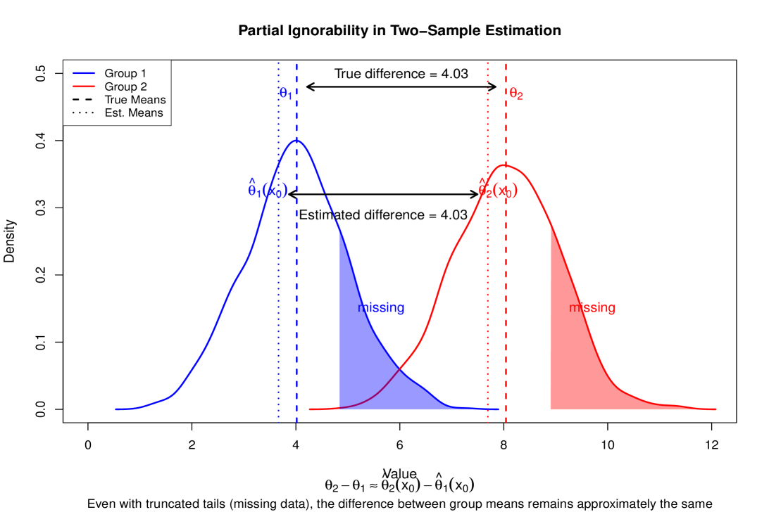
Figure 1: Even if the data are nonignorably missing (shaded parts are systematically on the upper end of the distributions), estimated treatment effects can still be valid under relative ignorability (nonignorable missingness affects both groups equally; both distributions are censored at the 80% quantile).

This concept has been discussed in earlier work at the interface of Causal Inference and Reinforcement Learning. For example, consider the situation where we wish to optimize cancer treatment by adaptively selecting actions based on observed covariates at each timepoint. This problem is an active area of research development (see, for example, Bleile (2023); Yu et al. (2019); Zhang et al. (2021), though many other examples exist). A comprehensive introduction to the methodological landscape is available in Kosorok and Moodie (2015), which highlights $Q$-learning as a popular approach to the optimal dynamic treatment policy selection problem in cancer research. An example from Bleile (2023) shows how the concept of relative ignorability can be applied to adaptive treatment strategy as follows: Suppose that applying actions $a=1,2$ respectively to a specific subject will truly result in counterfactual outcomes of $3$ and $5$, respectively, so that action 1 is truly better than action 2 for that individual. Suppose we have two predictive systems: i) $Q^{(1)}$, which estimates these counterfactual outcomes as $10,50$, and ii) $Q^{(2)}$, which estimates them as $4,3.5$. Although $Q^{(2)}$ is more accurate in terms of mean squared error, $Q^{(1)}$ is better for selecting an optimal treatment, because it ranks the potential outcomes correctly. relative ignorability becomes relevant when we realize that all datasets are incomplete; due to the interconnectedness of the universe, we can never truly measure all variables which affect the outcome - every statistical model is a closed-system approximation to a truly nonlinear dynamic system. The key for successful modelling is to ensure that the excluded variables do not matter for decision-making, i.e. they are partially ignorable. In the predictive system example, then, $Q^{(1)}$ is fit to a dataset where the excluded variables are ignorable for the purpose of absolute prediction, whereas $Q^{(2)}$ is fit to a dataset where the unmeasured variables are ignorable for the purposes of relative prediction, which is more relevant to decision-making.

The concept of relative ignorability refines the statistical theory of ignorability developed in previous work. Heitjan (1994) introduced the concept of nonignorable missingness, and various extensions and applications have been discussed. For instance Xie et al. (2004); Xie and Qian (2009); Troxel et al. (2004); Xie et al. (2003); Ma et al. (2002) developed a framework for sensitivity analysis, and Heitjan and Rubin (1991); Zhang et al. (2007); Zhang and Zhang (2006) develop an extension to coarse data. A thorough exploration of the estimation issues inherent with nonignorability was produced by Diggle and Kenward (1994). Mohan et al. (2013) framed the Causal Inference problem as a missing data issue; Hernán and Robins (2010) provides a comprehensive introduction to Causal Inference with this perspective in mind.

2 Background and Notation

Definition 1 (Stochastic Decision Process).

A Stochastic Decision Process is characterized by a 4-tuple $(\Omega,\mathcal{A},P,\rho)$ where:

• $\Omega$ is the set of possible states, known as the state space, from which states $(X\in\Omega)$ are drawn from probability distribution $F_{X}(x)$ on $\Omega$, where $F_{X}(x)=Pr(X\leq x)$.

• $\mathcal{A}$ is the set of possible actions that one can take at each iteration , known as the action space, from which actions $(A\in\mathcal{A})$ are drawn from probability distribution $\pi(a,X)$ on $\Omega\times\mathcal{A}$, where $\pi(A=a|X=x)$ denotes the probability of selecting action $a$ given the observed state $x$.

• $P:\Omega\times\mathcal{A}\times\Omega\rightarrow[0,1]$ is a probability distribution which governs the state transition dynamics, where
  $P(x^{\prime}|x,a)$ represents the probability of transitioning to state $x^{\prime}$ when taking action $a$ in state $x$

• $\rho:\Omega\rightarrow\mathbb{R}$ is the reward function, where $\rho(X)$ represents the intrinsic reward of being in state $X$.

Repeated draws from $X,A$ constitute the MDP itself, and for each draw of $X=x$, the value $r=\rho(x)$ is computed. Draws are indexed by $j$ and values are denoted $\{x_{j},a_{j},r_{j}\}$. This set of draws is also known as a filtration on $\Omega$.

1. Initialize $x_{0},a_{0}$. Set $j=0$

2. Apply $a_{j}$. Draw $x_{j+1}\sim P(x_{j},a_{j})$

3. Compute $r_{j+1}=\rho(x_{j+1})$

4. Set $j=j+1$ and return to 2.

We place the usual technical requirements on the stochastic process:

1. $\rho$ is bounded and measureable

2. $\Omega$ is a complete metric space

3. The state transition dynamics $P$ are measureable for all $x\in\Omega$.

These assumptions ensure that the set of draws from $\{X,A\}$ constitute a proper filtration. We use the notational shorthand $\mathcal{F}_{J}$ to denote the filtration up to $j=J$.(Puterman, 1994)

For the conventional results in RL to hold, the stochastic must also satisfy the Markov property,i.e. it must be a Markov Decision Process. (Bellman, 1957)

Conventional Reinforcement Learning notation does not differentiate $R$ and $\rho$, using lowercase $r$ interchangeably as a random variable, a fixed value, or a function. This dual usage of $r$ as a variable and a function is imprecise and can be confusing; we use a refined notation here for clarity.

Assuming the usual goal of maximizing some discounted reward function $r_{j}+\gamma r_{j+1}+\gamma^{2}r_{j+2}\dots$, the standard learning conditions are that $\sum_{j}\gamma_{j}=\infty$, $\sum_{j}\gamma_{j}^{2}<\infty$ and each state-action pair is visited infinitely often (exploration condition); i.e. the state transition probabilities $P$ and the action selection probability $\pi$ are defined such that $P(X,X^{\prime})>0\forall X,X^{\prime}\in\Omega\times\Omega$ . Throughout this paper we use $x,x^{\prime}$ to denote state and next state, per conventional Reinforcement Learning notation. Subscripts $o,m$ denote observed and missing components of the subscripted variable; e.g. $z_{m},z_{o}$ are the missing and observed parts of $z=(z_{o},z_{m})$.

3 Relative ignorability

3.1 Definition

Let $Z=(X,A)$ be the state-action pair. So, $Z\in\Omega\times\mathcal{A}$; for notational shorthand we use $\Omega\times\mathcal{A}:=\zeta$. Let $Z_{j}$ be the matrix of draws of $Z=(X,A)$ up until time $j$.

Suppose we wish to fit some estimation model $Q(\theta)$ to our data, where $\theta$ are the parameters of $Q$. One typically does this by using the data $Z$ to derive estimates $\hat{\theta}$ of $\theta$ which optimize, in whole or in part, a function $d(\tilde{\theta},Z):\Theta\times\zeta\rightarrow\mathbb{R}$ which measures how well a set of proposed values of $\tilde{\theta}\in\Theta$ fit the data $Z$ under $Q$. For example, in the two sample $z$-test, $\theta=(\mu_{1},\mu_{2})$ where $\mu_{1},\mu_{2}$ are the groupwise means, $Q(Z)$ is a normal distribution with mean $\mu_{1}\mathbb{1}(a=1)+\mu_{2}\mathbb{1}(a=2)$, and $d(\theta,Z)$ is the inverse liklihood. The key insight of this paper is that the accuracy of the estimates themselves are unimportant for the purposes of estimated group differences; it is the accuracy of a transformation of the parameters $\psi=g(\theta)$, where $g:\Theta\rightarrow\Psi s.t.g(\theta)=\mu_{2}-\mu_{1}$ which is imperative to estimate. Stated another way, in order to achieve actionable insights from $Z$, the accuracy of an estimate $\hat{\mu}_{2}$ of $\mu_{2}$ is important only relative to the accuracy of $\hat{\mu}_{1}$.

This realization allows us to relax the Markov assumptions in certain cases because $\Psi$ might not be as “big” as $\Theta$: For example, in the $z$-test case, requiring accurate $\hat{\mu}_{1},\hat{\mu}_{2}$ is more restrictive than requiring accurate $\hat{\delta}$, where $\delta=\mu_{2}-\mu_{1}$. This is highlighted in Figure 1: Here, the observed distributions are shifted to the left from the true ones, but this does not affect the actionable insight of group difference estimate. Indeed, the observed distributions could appear anywhere on the real axis, allowing an arbitrarily large bias on $\hat{\mu}_{1},\hat{\mu}_{2}$, and as long as that bias affects both groups equivalently, the actionable insight of which group’s mean is higher is still valid. In this case we would say that the missingness in $Z$ which incurs such a bias is relatively nonignorable with respect to $a$, the group indicator.

Note that in the above example, $\hat{\mu}_{1}$ and $\hat{\mu}_{2}$ functions of $Z_{o}$ - typically the group means computed across the observed data. More generally, for fixed $Q,\theta$, we can define an estimating function $g_{Q\theta}:\zeta\rightarrow\Psi s.t.g_{Q\theta}(Z)$ returns $\hat{\psi}$, the estimates of $\psi$ given $Z$ under fixed $Q,\theta$. Using a small notational abuse for the purpose of intuition, we use $\hat{g}(\theta,Z)$ to denote $\hat{\psi}$.

Assuming $\hat{g}(\theta,Z)$ is a consistent estimator of $g(\theta)$, and that $g$ satisfies certain measure-theoretic properties, relative ignorability is presented in Definition 2.

Definition 2 (relative ignorability).

$z_{m}\subset Z$ is said to be relatively ignorable with respect to an estimator $\hat{g}(\theta,Z)$ of $g(\theta),\theta\in\Theta$ if and only if $\hat{g}(\theta,Z/\ z_{m})=\hat{g}(\theta,Z)$.

Another way to say this is that $z_{m}$ is ignorable relative to $\hat{g}$ if and only if $\hat{g}$ is functionally independent of $z_{m}$. If we say that $z_{m}$ is relatively ignorable without specifying some estimator, this is shorthand for “There exists some estimator $\hat{g}(\theta)$ such that $z_{m}$ is relatively ignorable with respect to $\hat{g}(\theta,Z)$”.

Relative ignorability is meaningfully defined only for $g$ which satisfy two principles: i) Functional independence of missingness itself and ii) identifiability. Functional independence of missigness requires that $g$ behaves the same way for the missing and observed parts of $Z$; we need to know that censoring an element of $Z$ (transforming an observed part $z_{o}$ of $Z$ to be missing, i.e. $z_{o}\rightarrow z_{m}$) does not change what $\hat{g}$ does with it; $\hat{g}$ doesn’t care whether $z\subset Z$ is missing before deciding what output to return. A simple counterexample would be if we defined $g$ as $g(\theta,Z)=\theta Z\cdot M^{\prime}$, where $M$ is a matrix of missingness indicators on $Z$, $M^{\prime}$ is the transpose of $M$, and $\cdot$ represents matrix multiplication. This is different from functional independence of $z_{m}$, which would state that for two different values of $Z_{m}$ denoted $z^{\prime}_{m},z^{\prime\prime}_{m}$, we have $\hat{g}(z_{o}\cup z^{\prime}_{m},\theta)=\hat{g}(z_{o}\cup z^{\prime\prime}_{m},\theta)$ for arbitrary $\theta\in\Theta$.

Identifiability requires that $g^{-1}(\theta)$ is meaningfully defined; two different values of $\theta$ cannot produce the same output from $g$. Figure 2 illustrates this concept for the case where $\theta$ has only one parameter ($\Theta=\mathbb{R}$).

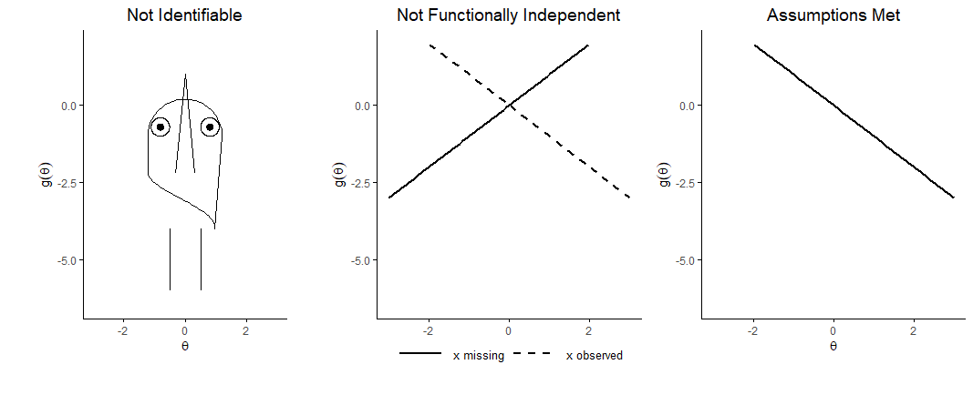
Figure 2: The transformation $g(\theta)$ must be identifiable and functionally independent of missingness.

Relative ignorability can be further generalized to a concept of weak relative ignorability, which only requires consistency of $\hat{g}(\theta,Z/z_{m})$. Weak relative ignorability is less restrictive than relative ignorability, requiring equality of estimator computed as a function of $Z/z_{m}$ (Z without the missing part $z_{m}$) with $\theta$ only under expectation. This second concept can be used to relax the Markov requirements on the optimal convergence of the Q-learning framework.

Definition 3 (Weak relative ignorability).

$z_{m}\subset Z$ is said to be relatively ignorable with respect to a consistent estimator $\hat{g}(\theta,Z)$ of $g(\theta)\in\Theta$ if and only if $\mathbb{E}[\hat{g}(\theta,Z/z_{m})]=\mathbb{E}[\hat{g}(\theta,Z)]=g(\theta)$, i.e. if the estimator $\hat{g}(\theta)$ is still consistent when computed without $z_{m}$. This can also be phrased as “$z_{m}$ is weakly ignorable relative to $\hat{g}$”.

Note that the definition of $z_{m}$ is very general. For example, $z_{m}$ could be an entire column vector such as a covariate. $z_{m}$ might also be part of the outcome vector. In the $z$-test example, then $\mathbb{E}[\hat{\mu}_{1}]=\mathbb{E}[\hat{\mu}_{2}]$ only when the outcome vector is partially ignorable with respect to the difference in groupwise means $\hat{g}(\theta,Z)=\frac{1}{n_{2}}\sum_{i\in 1:J}x_{i}\mathbb{1}(a_{i}=2)-\frac{1}{n_{1}}\sum_{i\in 1:J}x_{i}\mathbb{1}(a_{i}=1)$ as an estimator of $g(\theta):\mu_{2}-\mu_{1}$, where $n_{1}$ counts the number of occurrences of $a=1$, and $n_{2}$ is defined similarly, and $J$ is the number of observations of $Z$ so far. The entirety of frequentist statistical hypothesis testing can be similarly framed in terms of relative ignorability of the outcome variable with respect to the input variable in question: In the $z$-test example above, the input variable is a categorical action vector $a$, but the relative ignorability framework is general enough to incorporate multivariate or continuous definitions of $z_{m}$.

3.2 Main Results

Under the relative ignorability condition and standard stochastic approximation conditions , Causal Q-learning with Marginal Structural Model estimation converges to the unique fixed point $Q^{*}$ of the expected Bellman optimality operator with probability 1. Our proof of this follows the same general schema used by Bellman’s original paper, leveraging the Contraction Mapping Theorem as well as the Banach fixed-Point Theorem: We show that an extended Bellman update equation which accommodates partially ignorable missing components via a marginal structurual model approach (Equation 1) still gives us the eventual optimal function $Q$. We do this in two steps: First, we show that applying this generalized Bellman equation causes $Q$ to converge in $j$ to a fixed point in function space by the Contraction Mapping Theorem (Lemma 1). Next, we use a generalized form of the Robbins-Munro Stochastic Approximation theorem (Jaakkola et al., 1994; Robbins and Monro, 1951) to show that that fixed point is an optimum. These results taken together prove our result. Figure 3 shows a graphic visualization of the proof, and an interactive version which links nodes and edges to specific text in the paper is also available at the following url: https://merlinbleile.shinyapps.io/relativeqlearningproof/

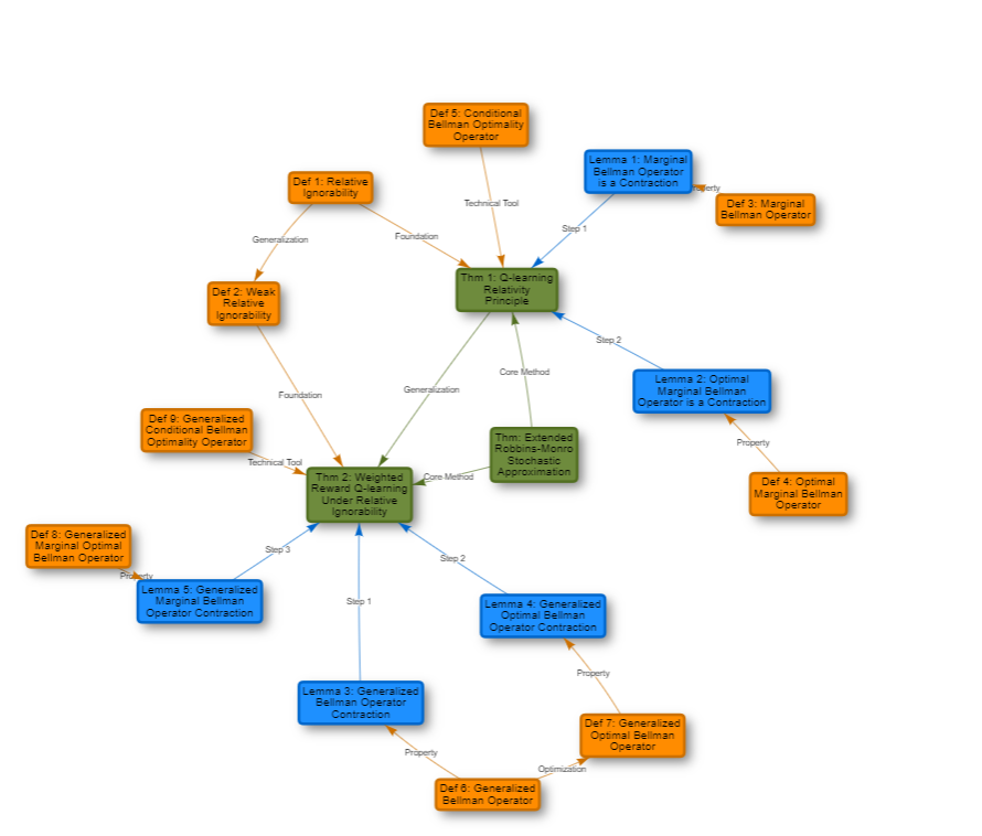
Figure 3: Network diagram illustrating the proof structure.

$$T_{o}Q(x_{o},a)=r+\gamma\sum_{x_{o}^{\prime}}\int_{\Omega_{m}}P(x_{o}^{\prime}|x_{o}\cup x_{m},a)\mu(x_{m}|x_{o},a)dx_{m}\sum_{a^{\prime}}Q(x_{o}^{\prime},a^{\prime})$$ (1)

Note that the generalized Bellman update operator $T_{o}$ is defined on the refined filtration $\mathcal{F}_{o}\subset\mathcal{F}$, corresponding to the observed part of $\mathcal{F}$. Intuitively, it is obvious that $\mathcal{F}_{o}$ is a filtration (though, importantly, it might not be Markov). The technical argument is that since $\Omega$ is complete, we know $Z_{o}\subset Z$ is measurable on $\Omega_{o}\subset\Omega$, which satisfies the definition of a filtration. The observed values $r_{o}$ are the same as the $r$ from the complete filtration $\mathcal{F}$, with an important nuance. First note that in the complete filtration, each value of $r$ is a draw from the random variable $R=\rho(X)$; so $R=r+\varepsilon$, where $\varepsilon$ is a random variable which encapsulates the stochastic noise on the MDP.Since $\mathcal{F}$ is Markov, $\mathbb{E}[\varepsilon_{j}|\mathcal{F}_{j}]=0$. Conversely, consider the observed filtration, with $R_{o}=r_{o}+\varepsilon_{o}$ similarly defined, Now, the variability due to $z_{m}$ is now attributed to $\varepsilon_{o}$; if missingness of $z_{m}$ is nonignorable in the classic sense of the word, then $\mathbb{E}[\varepsilon_{oj}|\mathcal{F}_{oj}]\neq 0$.

The new Bellman update equation is defined in Equation 1. Here $r$ is the value $r=\rho(x^{\prime})$ where $x^{\prime}$ is the draw from $X^{\prime}\sim P(X=x,A=a)$, i.e. what actually happened at the next timepoint (commonly denoted $r(X,a)$ for state $s$ and action$a$ under a policy $\pi$). Assume also that the vector of missing elements of $z$, denoted $z_{m}$, is partially ignorable with respect to the reward function $\rho$. This assumption will allow the asymptotics of the Bellman operator defined in Equation 2 to behave as desired: $T^{\pi}Q(Z_{o})$ will unbiasedly approximate $T^{\pi}Q(Z)$. Using these properties, we can show that the marginal optimality operator in Equation 13 is a contraction mapping (Lemma 1).

Definition 4 (Marginal Bellman Operator).

$$B^{\pi}Q(Z)=\int_{\Omega_{m}}T^{\pi}Q(Z)\mu(z_{m})dZ_{m}$$ (2)

Lemma 1.

The marginal Bellman operator $B^{\pi}$ is a contraction mapping.

Proof.

We know using Bellman’s original result (1957) that $TQ(Z)$ is a contraction mapping with contraction factor $\gamma$ when applied to draws $Z$ from the complete filtration $\mathcal{F}$ (Equation 3). We first want to establish that $TQ(Z_{o})$ is also a contraction mapping when applied to draws from the observed filtration $\mathcal{F}_{o}$.

$$\|TQ_{1}-TQ_{2}\|_{\infty}\leq\gamma\|Q_{1}-Q_{2}\|_{\infty}$$ (3)

Note that while the observed filtration $\mathcal{F}_{o}$ may not satisfy the Markov property, the weak relative ignorability assumption ensures that when we take the expectation with respect to the missing components $z_{m}$, the resulting operator inherits the contraction property from the complete Bellman operator with an asymptotically vanishing error term. This is formalized as follows:

$$\|B^{\pi}Q_{1}-B^{\pi}Q_{2}\|_{\infty} =\left\|\int_{\Omega_{m}}T^{\pi}Q_{1}(Z_{o}\cup z_{m})\mu(z_{m}|Z_{o})dz_{m}-\int_{\Omega_{m}}T^{\pi}Q_{2}(Z_{o}\cup z_{m})\mu(z_{m}|Z_{o})dz_{m}\right\|_{\infty}$$ (4)

$$=\left\|\int_{\Omega_{m}}[T^{\pi}Q_{1}(Z_{o}\cup z_{m})-T^{\pi}Q_{2}(Z_{o}\cup z_{m})]\mu(z_{m}|Z_{o})dz_{m}\right\|_{\infty}$$ (5)

Using Jensen’s inequality, we have:

$$\left\|\int_{\Omega_{m}}[T^{\pi}Q_{1}(Z_{o}\cup z_{m})-T^{\pi}Q_{2}(Z_{o}\cup z_{m})]\mu(z_{m}|Z_{o})dz_{m}\right\|_{\infty} \leq\int_{\Omega_{m}}\|T^{\pi}Q_{1}(Z_{o}\cup z_{m})-$$ (7)

$$T^{\pi}Q_{2}(Z_{o}\cup z_{m})\|_{\infty}\mu(z_{m}|Z_{o})dz_{m}$$ (8)

$$\leq\int_{\Omega_{m}}\gamma\|Q_{1}-Q_{2}\|_{\infty}\mu(z_{m}|Z_{o})dz_{m}$$ (9)

$$=\gamma\|Q_{1}-Q_{2}\|_{\infty}\int_{\Omega_{m}}\mu(z_{m}|Z_{o})dz_{m}$$ (10)

$$=\gamma\|Q_{1}-Q_{2}\|_{\infty}$$ (11)

∎

Now we know that there is a fixed point, but we still need two know two things: i) What is the fixed point? ii) Is the fixed point a maximum, minimum, or something else? We will start with point i) is formalised in Lemma 2, stating that the marginal Bellman optimality equation in Equation 12 is the fixed point of the relative Bellman estimator.

$$B^{*}Q(x_{o},a)=\rho(x^{\prime})+\gamma\sum_{x^{\prime}_{o}}P(x^{\prime}_{o}|X,a)\max_{a^{\prime}}Q(x^{\prime}_{o},a^{\prime})$$ (12)

Definition 5 (Optimal Marginal Bellman Operator).

$$B^{*}Q(x,a)=\int_{\Omega_{m}}T^{*}Q(x,a)\mu(z_{m})dz_{m}$$ (13)

Lemma 2.

The marginal Bellman optimality operator $B^{*}$ is a contraction mapping in the max-norm.

Lemma 2.

This can be shown using the exact same steps as the proof of Lemma 1, using the contraction mapping properties of the original Bellman optimality operator Bellman (1957). ∎

Next, we wish to show convergence of MSM-augmented Q-learning using the extended Robins-Monro stochastic approximation theorem. The original version of this theorem states for an MDP $\mathcal{F}$ on $Q$ with bounded variance on the noise terms, a contraction mapping $\mathcal{H}$ on $\mathcal{F}$ converges to its optimum $\mathcal{H}^{*}$ across trial iterations $j$. If we could apply this result to our pet contraction mapping (set $\mathcal{H}=B^{\pi}$), then the theorem is proved.

Unfortunately there are some issues: Most notably, $\mathcal{F}_{o}$ might not be Markov, due to potential nonignorability in $z_{m}$. We would also need bounded variance on the error terms. To overcome these issues, we use instead a generalized version of this theorem, which relaxes the assumptions on the error terms: Jaakkola et al. (1994) showed that the result still holds for non-Markov filtrations as long as the error terms are asymptotically zero, i.e. in expectation with respect to the unobserved part of $X$. Specifically, this requires that $\mathbb{E}[\varepsilon_{oj}|\mathcal{F}_{oj}]\xrightarrow[j\to\infty]{\text{a.s.}}0$.

Theorem 3 (Q-learning Relativity Principle, Precise Definition).

Suppose the following:

• $z_{m}$ is ignorable relative to $\hat{\rho}(X)$ (where $\theta$ are the parameters of $Q$)

• $z_{m}\subset X$ (rewards are not missing)

• The standard stochastic approximation conditions on $\gamma$ are applicable

then, Q-learning with MSMs converges to the unique fixed point $Q^{*}$ of the expected Bellman optimality operator with probability 1.

Theorem 3.

Let $\mathcal{F}$ be a filter on $Q(\theta)$ with observed subset $\mathcal{F}_{o}$ as defined as above. Suppose that at each iteration, some $z_{jm}\subset X\subset Z$ are missing, but that these $z_{jm}$ are ignorable relative to $T^{*}Q(z_{j},\theta)$, taken as a function of $\theta$. Let $\mathcal{F}_{o}$ be the observed part of $\mathcal{F}$ (recall that we have previously established that $\mathcal{F}_{o}\subset\mathcal{F}$ is a filter), and let $\varepsilon^{o}_{j}$ be the corresponding error term for the $j^{th}$ iteration of $\mathcal{F}_{o}$. We know that $F_{o},F^{*}$ are contraction mappings by Lemmas 1-2, and by definition of $\gamma$ (standard $Q$-learning conditions), we have $\sum_{j}\gamma_{j}=\infty,\sum_{j}\gamma^{2}_{j}<\infty$. So, it suffices to show that $\mathbb{E}[\varepsilon^{o}_{j}|\mathcal{F}_{o}]\xrightarrow[j\to\infty]{\text{a.s.}}0$ with bounded variance.

To show this, we introduce a conditional relative Bellman operator $\hat{B}^{*}$ for the observed process $\mathcal{F}_{o}$ and show that $\hat{B}^{*}Q_{j}(x_{oj},a_{j})=\mathbb{E}[B^{*}Q_{j}|\mathcal{F_{o}}]$, in which case it follows from basic algebraic operations that the error terms form the required martingale difference sequence and the result is proved.

Definition 6 (Conditional Bellman Optimality Operator).

$$\hat{B}^{*}Q_{j}(x_{j,o},a_{j})=\mathbb{E}[r_{j+1}+\gamma\max_{a^{\prime}}Q_{j}(x_{j+1,o},a^{\prime})|x_{j,o},a_{j},\mathcal{F}_{o,j}]$$ (14)

Then,

$$\hat{B}^{*}Q_{j}(x_{j,o},a_{j}) =\mathbb{E}[r_{j+1}+\gamma\max_{a^{\prime}}Q_{j}(x_{j+1,o},a^{\prime})|x_{j,o},a_{j},\mathcal{F}_{o,j}]$$ (15)

$$=\mathbb{E}[\mathbb{E}[r_{j+1}+\gamma\max_{a^{\prime}}Q_{j}(x_{j+1,o},a^{\prime})|x_{j,o},x_{j,m},a_{j},\mathcal{F}_{o,j}]|x_{j,o},a_{j},\mathcal{F}_{o,j}]$$ (16)

$$=\int_{\Omega_{m}}\mathbb{E}[r_{j+1}+\gamma\max_{a^{\prime}}Q_{j}(x_{j+1,o},a^{\prime})|x_{j,o},x_{m},a_{j},\mathcal{F}_{o,j}]\mu(x_{m}|x_{j,o},a_{j},\mathcal{F}_{o,j})dx_{m}$$ (17)

$$=\int_{\Omega_{m}}T^{*}Q_{j}(x_{j,o}\cup x_{m},a_{j})\mu(x_{m}|x_{j,o},a_{j},\mathcal{F}_{o,j})dx_{m}$$ (18)

$$=\mathbb{E}[B^{*}Q_{j}(x_{j,o},a_{j})|\mathcal{F}_{o,j}]$$ (19)

as required.

∎

Next we wish to relax the assumptions somewhat by allowing missingness in the rewards (remove $z_{m}\subset X$ requirement) and by removing the requirement of the MSM weights. To do this, we now require that $z_{m}$ is ignorable relative to the Bellman operator, and apply weights only according to missingess probability (Theorem 4).

Theorem 4 (Weighted Reward Q-learning Under Relative Ignorability).

Consider a modified Q-learning update rule with weighted rewards:

$$Q(z_{j,o},a_{j})\leftarrow Q(z_{j,o},a_{j})+\alpha_{j}\left[\frac{M_{j}\cdot r_{j+1}}{P(M_{j}=1|z_{j,o},a_{j})}+\gamma\max_{a^{\prime}}Q(z_{j+1,o},a^{\prime})-Q(z_{j,o},a_{j})\right]$$

where:

• $M_{j}$ is a missingness indicator such that $M_{j}=1$ when $r_{j+1}$ is observed and $M_{j}=0$ otherwise

• $P(M_{j}=1|z_{j,o},a_{j})$ is the probability that $r_{j+1}$ is observed given $z_{j,o}$ and $a_{j}$

Suppose that:

1. $z_{jm}$ is weakly relatively ignorable with respect to $\hat{g}(Z,\theta):=T^{*}Q(Z_{j},\theta)$

2. The missingness mechanism for rewards satisfies $P(M_{j}=1|z_{j,o},a_{j},r_{j+1})=P(M_{j}=1|z_{j,o},a_{j})$ (i.e., the missingness is ignorable with respect to the reward value itself)

3. $P(M_{j}=1|z_{j,o},a_{j})>\delta>0$ for all $z_{j,o},a_{j}$ (positivity condition)

4. The standard stochastic approximation conditions on $\alpha_{j}$ and $\gamma$ are applicable

Then, the weighted reward Q-learning algorithm converges to the unique fixed point $Q^{*}$ of the expected Bellman optimality operator with probability 1.

The proof of Theorem 4 follows the same structure as before, with some additional expected values included. First we define a generalized Bellman operator $T_{o}^{G}Q(Z_{o},a)$ and show that this $T_{o}^{G}Q(Z_{o},a)$ is a contraction mapping.

$$T_{o}^{G}Q(Z_{o},a) :=\int_{\Omega_{m}}\mathbb{E}[\rho(x^{\prime})|Z_{o},z_{m},a]\mu(z_{m}|Z_{o},a)dz_{m}+$$ (20)

$$\gamma\sum_{z_{o}^{\prime}}\int_{\Omega_{m}}P(z_{o}^{\prime}|Z_{o}\cup z_{m},a)\mu(z_{m}|Z_{o},a)dz_{m}\sum_{a^{\prime}}Q(z_{o}^{\prime},a^{\prime})$$ (21)

The key difference between $T_{o}^{G}$ and $T_{o}$ is that $T_{o}^{G}$ includes an expectation over the reward term, which is what allows us to relax the assumption of non-missing rewards. Using a similar argument as before, we can show that $T_{o}^{G}Q(Z_{o},a)$ is a contraction mapping:

$$\|T_{o}^{G}Q_{1}-T_{o}^{G}Q_{2}\|_{\infty} =\Big{\|}\gamma\sum_{z_{o}^{\prime}}\int_{\Omega_{m}}P(z_{o}^{\prime}|Z_{o}\cup z_{m},a)\mu(z_{m}|Z_{o},a)dz_{m}\sum_{a^{\prime}}[Q_{1}(z_{o}^{\prime},a^{\prime})-Q_{2}(z_{o}^{\prime},a^{\prime})]\Big{\|}_{\infty}$$ (22)

$$\leq\gamma\sum_{z_{o}^{\prime}}\int_{\Omega_{m}}P(z_{o}^{\prime}|Z_{o}\cup z_{m},a)\mu(z_{m}|Z_{o},a)dz_{m}\|Q_{1}-Q_{2}\|_{\infty}$$ (23)

$$=\gamma\|Q_{1}-Q_{2}\|_{\infty}\sum_{z_{o}^{\prime}}\int_{\Omega_{m}}P(z_{o}^{\prime}|Z_{o}\cup z_{m},a)\mu(z_{m}|Z_{o},a)dz_{m}$$ (24)

$$=\gamma\|Q_{1}-Q_{2}\|_{\infty}$$ (25)

The rest of the proof structure is the same as before, with the following generalized operators:

Definition 7 (Generalized Optimal Bellman Operator).

$$T_{o}^{G*}Q(Z_{o},a) =\int_{\Omega_{m}}\mathbb{E}[\rho(x^{\prime})|Z_{o},z_{m},a]\mu(z_{m}|Z_{o},a)dz_{m}+$$ (26)

$$\gamma\sum_{z_{o}^{\prime}}\int_{\Omega_{m}}P(z_{o}^{\prime}|Z_{o}\cup z_{m},a)\mu(z_{m}|Z_{o},a)dz_{m}\max_{a^{\prime}}Q(z_{o}^{\prime},a^{\prime})$$ (27)

Definition 8 (Generalized Marginal Optimal Bellman Operator).

$$B^{G*}Q(Z)=\int_{\Omega_{m}}T^{G*}Q(Z)\mu(z_{m})dz_{m}$$ (28)

Definition 9 (Generalized Conditional Bellman Optimality Operator).

$$\hat{B}^{G*}Q_{j}(Z_{j,o},a_{j}) =$$ (29)

$$\mathbb{E}\left[\int_{\Omega_{m}}\mathbb{E}[\rho(x^{\prime})|Z_{j,o},z_{m},a_{j}]\mu(z_{m}|Z_{j,o},a_{j})dz_{m}+\gamma\max_{a^{\prime}}Q_{j}(Z_{j+1,o},a^{\prime})\Bigg{|}Z_{j,o},a_{j},\mathcal{F}_{o,j}\right]$$ (30)

Lemma 5 (Generalized Bellman Operator Contraction).

The generalized Bellman operator $T_{o}^{G}$ is a contraction mapping.

Proof.

For any two Q-functions $Q_{1}$ and $Q_{2}$, we have:

$$\|T_{o}^{G}Q_{1}-T_{o}^{G}Q_{2}\|_{\infty} =\Big{\|}\gamma\sum_{z_{o}^{\prime}}\int_{\Omega_{m}}P(z_{o}^{\prime}|Z_{o}\cup z_{m},a)\mu(z_{m}|Z_{o},a)dz_{m}\sum_{a^{\prime}}[Q_{1}(z_{o}^{\prime},a^{\prime})-Q_{2}(z_{o}^{\prime},a^{\prime})]\Big{\|}_{\infty}$$ (31)

$$\leq\gamma\sum_{z_{o}^{\prime}}\int_{\Omega_{m}}P(z_{o}^{\prime}|Z_{o}\cup z_{m},a)\mu(z_{m}|Z_{o},a)dz_{m}\|Q_{1}-Q_{2}\|_{\infty}$$ (32)

$$=\gamma\|Q_{1}-Q_{2}\|_{\infty}\sum_{z_{o}^{\prime}}\int_{\Omega_{m}}P(z_{o}^{\prime}|Z_{o}\cup z_{m},a)\mu(z_{m}|Z_{o},a)dz_{m}$$ (33)

$$=\gamma\|Q_{1}-Q_{2}\|_{\infty}$$ (34)

where the last equality follows because $\sum_{z_{o}^{\prime}}\int_{\Omega_{m}}P(z_{o}^{\prime}|Z_{o}\cup z_{m},a)\mu(z_{m}|Z_{o},a)dz_{m}=1$, since $P$ is a probability distribution. ∎

Lemma 6 (Generalized Optimal Bellman Operator Contraction).

The generalized optimal Bellman operator $T_{o}^{G*}$ is a contraction mapping in the max-norm.

Proof.

Following a similar approach as in Lemma 5, for any two Q-functions $Q_{1}$ and $Q_{2}$:

$$\|T_{o}^{G*}Q_{1}-T_{o}^{G*}Q_{2}\|_{\infty} =\Big{\|}\gamma\sum_{z_{o}^{\prime}}\int_{\Omega_{m}}P(z_{o}^{\prime}|Z_{o}\cup z_{m},a)\mu(z_{m}|Z_{o},a)dz_{m}[\max_{a^{\prime}}Q_{1}(z_{o}^{\prime},a^{\prime})-\max_{a^{\prime}}Q_{2}(z_{o}^{\prime},a^{\prime})]\Big{\|}_{\infty}$$ (35)

Using the property that $|\max_{a}f(a)-\max_{a}g(a)|\leq\max_{a}|f(a)-g(a)|$, we have:

$$\|T_{o}^{G*}Q_{1}-T_{o}^{G*}Q_{2}\|_{\infty} \leq\Big{\|}\gamma\sum_{z_{o}^{\prime}}\int_{\Omega_{m}}P(z_{o}^{\prime}|Z_{o}\cup z_{m},a)\mu(z_{m}|Z_{o},a)dz_{m}\max_{a^{\prime}}|Q_{1}(z_{o}^{\prime},a^{\prime})-Q_{2}(z_{o}^{\prime},a^{\prime})|\Big{\|}_{\infty}$$ (37)

$$\leq\gamma\|Q_{1}-Q_{2}\|_{\infty}\sum_{z_{o}^{\prime}}\int_{\Omega_{m}}P(z_{o}^{\prime}|Z_{o}\cup z_{m},a)\mu(z_{m}|Z_{o},a)dz_{m}$$ (38)

$$=\gamma\|Q_{1}-Q_{2}\|_{\infty}$$ (39)

∎

Lemma 7 (Generalized Marginal Bellman Operator Contraction).

The generalized marginal Bellman operator $B^{G*}$ is a contraction mapping.

Proof.

For any two Q-functions $Q_{1}$ and $Q_{2}$:

$$\|B^{G*}Q_{1}-B^{G*}Q_{2}\|_{\infty} =\left\|\int_{\Omega_{m}}T^{G*}Q_{1}(Z)\mu(z_{m})dz_{m}-\int_{\Omega_{m}}T^{G*}Q_{2}(Z)\mu(z_{m})dz_{m}\right\|_{\infty}$$ (40)

$$=\left\|\int_{\Omega_{m}}[T^{G*}Q_{1}(Z)-T^{G*}Q_{2}(Z)]\mu(z_{m})dz_{m}\right\|_{\infty}$$ (41)

By Jensen’s inequality:

$$\left\|\int_{\Omega_{m}}[T^{G*}Q_{1}(Z)-T^{G*}Q_{2}(Z)]\mu(z_{m})dz_{m}\right\|_{\infty} \leq\int_{\Omega_{m}}\|T^{G*}Q_{1}(Z)-T^{G*}Q_{2}(Z)\|_{\infty}\mu(z_{m})dz_{m}$$ (43)

$$\leq\int_{\Omega_{m}}\gamma\|Q_{1}-Q_{2}\|_{\infty}\mu(z_{m})dz_{m}$$ (44)

$$=\gamma\|Q_{1}-Q_{2}\|_{\infty}\int_{\Omega_{m}}\mu(z_{m})dz_{m}$$ (45)

$$=\gamma\|Q_{1}-Q_{2}\|_{\infty}$$ (46)

The last equality holds because $\mu(z_{m})$ is a probability distribution that integrates to 1. ∎

Proof of Theorem 4.

Let $\mathcal{F}$ be a filter on $Q(\theta)$ with observed subset $\mathcal{F}_{o}$ as defined earlier. Suppose that at each iteration, some $z_{jm}\subset Z$ may be missing, but these $z_{jm}$ are weakly relatively ignorable with respect to $\hat{g}(Z,\theta):=T^{*}Q(Z_{j},\theta)$.

By Lemmas 5, 6, and 7, we know that the generalized operators $T_{o}^{G}$, $T_{o}^{G*}$, and $B^{G*}$ are all contraction mappings. Additionally, the standard stochastic approximation conditions on $\gamma$ ensure that $\sum_{j}\gamma_{j}=\infty$ and $\sum_{j}\gamma^{2}_{j}<\infty$.

To complete the proof, we need to show that the error terms $\varepsilon_{j}^{G}$ satisfy $\mathbb{E}[\varepsilon_{j}^{G}|\mathcal{F}_{o,j}]\xrightarrow[j\to\infty]{\text{a.s.}}0$ with bounded variance.

We define the error terms as:

$$\varepsilon_{j}^{G}=r_{j+1}+\gamma\max_{a^{\prime}}Q_{j}(z_{j+1,o},a^{\prime})-\hat{B}^{G*}Q_{j}(z_{j,o},a_{j})$$ (47)

By the definition of $\hat{B}^{G*}$:

$$\mathbb{E}[\varepsilon_{j}^{G}|\mathcal{F}_{o,j}] =\mathbb{E}[r_{j+1}+\gamma\max_{a^{\prime}}Q_{j}(z_{j+1,o},a^{\prime})|\mathcal{F}_{o,j}]-\hat{B}^{G*}Q_{j}(z_{j,o},a_{j})$$ (48)

$$=\hat{B}^{G*}Q_{j}(z_{j,o},a_{j})-\hat{B}^{G*}Q_{j}(z_{j,o},a_{j})$$ (49)

$$=0$$ (50)

Thus, the error terms form a martingale difference sequence. Additionally, since the reward function $\rho$ is bounded, and the Q-function is bounded (as guaranteed by the contraction property), the error terms have bounded variance.

By the generalized Robbins-Monro stochastic approximation theorem (Jaakkola et al., 1994), Q-learning with these generalized operators converges to the unique fixed point $Q^{*}$ of the expected Bellman optimality operator with probability 1. ∎

4 Conclusion

Theorem 3 provides a formalized justification of what has already been shown empirically in application: Zhao et al. (2009) developed a Causal Reinforcement Learning structure for adaptive treatment designs which leveraged the Q-learning in tandem with Marginal Structural Modeling (MSM), as in Equation 1. Here, the authors estimated the integral in Equation 1 using standard weighting techniques which are characteristic of the MSM approach, and performed extensive simulations to validate the efficacy of the approach. This approach was validated on real data in a follow-up paper.(Zhao et al., 2011) The more general result, Theorem 4, uses relative ignorability to relax the Markov assumptions on convergence properties of $Q$-learning, generalizing some results in the theory of POMDPs.(Kaelbling et al., 1998)

There are clear avenues for further integration of the concept of relative ignorability with the existing literature on Causal Inference. For example, one might frame exchangability of treatment groups in terms of relative ignorability of missingness in a standardized dataset with respect to the treatment parameter.

In summary, we have established the concept of relative ignorability, and demonstrated its downstream theoretical implications for Reinforcement Learning. Our theoretical result shows specific conditions under which the Markov assumption can be relaxed in Q-learning. This novel framework for conceptualizing convergence provides clear pathways for extension, with high-impact implications in multiple fields.

References

- Bellman (1957) Bellman, R. (1957). Dynamic Programming. Princeton University Press, Princeton, NJ.
- Bleile (2023) Bleile, M. (2023). Optimizing tumor xenograft experiments using bayesian linear and nonlinear mixed modelling and reinforcement learning. SMU Dissertation Archives.
- Diggle and Kenward (1994) Diggle, P. and Kenward, M. G. (1994). Informative drop-out in longitudinal data analysis. Journal of the Royal Statistical Society: Series C (Applied Statistics), 43(1):49–93.
- Heitjan (1994) Heitjan, D. F. (1994). Ignorability in general incomplete-data models. Biometrika, 81(4):701–708.
- Heitjan and Rubin (1991) Heitjan, D. F. and Rubin, D. B. (1991). Ignorability and coarse data. The Annals of Statistics, pages 2244–2253.
- Hernán and Robins (2010) Hernán, M. A. and Robins, J. M. (2010). Causal Inference: What If. Chapman & Hall/CRC, Boca Raton, FL.
- Jaakkola et al. (1994) Jaakkola, T., Jordan, M. I., and Singh, S. P. (1994). Convergence of stochastic iterative dynamic programming algorithms. In Advances in Neural Information Processing Systems, pages 703–710.
- Kaelbling et al. (1998) Kaelbling, L. P., Littman, M. L., and Cassandra, A. R. (1998). Planning and acting in partially observable stochastic domains. Artificial Intelligence, 101(1-2):99–134.
- Kosorok and Moodie (2015) Kosorok, M. R. and Moodie, E. E. (2015). Adaptive Treatment Strategies in Practice: Planning Trials and Analyzing Data for Personalized Medicine. SIAM, Philadelphia, PA.
- Ma et al. (2002) Ma, G., Geng, Z., and Hu, F. (2002). Measuring ignorability in non-monotone non-parametric models. Journal of Multivariate Analysis, 80(2):279–295.
- Mohan et al. (2013) Mohan, K., Pearl, J., and Tian, J. (2013). Missing data as a causal and probabilistic problem. In Proceedings of the Twenty-Ninth Conference on Uncertainty in Artificial Intelligence, pages 802–811.
- Mongillo and Deneve (2014) Mongillo, G. and Deneve, S. (2014). Misbehavior of q-learning with delay-dependent rewards. Advances in Neural Information Processing Systems, 27.
- Puterman (1994) Puterman, M. L. (1994). Markov Decision Processes: Discrete Stochastic Dynamic Programming. John Wiley & Sons, New York.
- Robbins and Monro (1951) Robbins, H. and Monro, S. (1951). A stochastic approximation method. The Annals of Mathematical Statistics, 22(3):400–407.
- Singh et al. (2000) Singh, S., Jaakkola, T., Littman, M. L., and Szepesvári, C. (2000). Convergence results for single-step on-policy reinforcement-learning algorithms. Machine Learning, 38(3):287–308.
- Sutton and Barto (2018) Sutton, R. S. and Barto, A. G. (2018). Reinforcement Learning: An Introduction. MIT Press, Cambridge, MA.
- Troxel et al. (2004) Troxel, A. B., Ma, G., and Heitjan, D. F. (2004). An index of local sensitivity to nonignorability. Statistica Sinica, 14(4):1221–1237.
- Xie and Qian (2009) Xie, H. and Qian, Y. (2009). Local sensitivity analysis for nonignorability: A review. AStA Advances in Statistical Analysis, 93(2):215–230.
- Xie et al. (2004) Xie, H., Song, X., Tang, N. S., and Cook, R. J. (2004). Sensitivity analysis of non-ignorable missing data mechanism: Application to a longitudinal trial of COPD. Statistics in Medicine, 23(7):1153–1171.
- Xie et al. (2003) Xie, H., Qian, Y., and Qu, L. (2003). An index for local sensitivity to nonignorability in longitudinal modeling. Biometrics, 59(1):189–194.
- Yu et al. (2019) Yu, Z., Shen, Y., and Zeng, D. (2019). Inverse probability weighted estimation for the survival advantage of treatment regimes. Statistica Sinica, 29(3):1347–1367.
- Zhang and Zhang (2006) Zhang, M. and Zhang, B. (2006). A simple approach to evaluate the ignorable missingness in the analysis of longitudinal data. Statistics & Probability Letters, 76(14):1502–1508.
- Zhang et al. (2007) Zhang, S., Liu, G., and Wang, L. (2007). On the impact of missing data in longitudinal studies with informative dropout. Journal of Statistical Planning and Inference, 137(3):926–936.
- Zhang et al. (2021) Zhang, Y., Deng, X., Wang, Z., and Zhao, D. (2021). Reinforcement learning based recommender systems: A survey. ACM Computing Surveys, 54(11s):1–38.
- Zhao et al. (2009) Zhao, Y., Zeng, D., Socinski, M.A., and Kosorok, M.R. (2009). Reinforcement learning design for cancer clinical trials. Statistics in Medicine, 28(26):3294–3315.
- Zhao et al. (2011) Zhao, Y., Zeng, D., Socinski, M. A., and Kosorok, M. R. (2011). Reinforcement learning strategies for clinical trials in nonsmall cell lung cancer. Biometrics, 67(4):1422–1433.