Adversarial Subspace Generation for Outlier Detection in High-Dimensional Data

Abstract

Outlier detection in high-dimensional tabular data is challenging since data is often distributed across multiple lower-dimensional subspaces — a phenomenon known as the Multiple Views effect (MV). This effect led to a large body of research focused on mining such subspaces, known as subspace selection. However, as the precise nature of the MV effect was not well understood, traditional methods had to rely on heuristic-driven search schemes that struggle to accurately capture the true structure of the data. Properly identifying these subspaces is critical for unsupervised tasks such as outlier detection or clustering, where misrepresenting the underlying data structure can hinder the performance. We introduce Myopic Subspace Theory (MST), a new theoretical framework that mathematically formulates the Multiple Views effect and writes subspace selection as a stochastic optimization problem. Based on MST, we introduce $\mathbf{V}$-GAN, a generative method trained to solve such an optimization problem. This approach avoids any exhaustive search over the feature space while ensuring that the intrinsic data structure is preserved. Experiments on 42 real-world datasets show that using $\mathbf{V}$-GAN subspaces to build ensemble methods leads to a significant increase in one-class classification performance — compared to existing subspace selection, feature selection, and embedding methods. Further experiments on synthetic data show that $\mathbf{V}$-GAN identifies subspaces more accurately while scaling better than other relevant subspace selection methods. These results confirm the theoretical guarantees of our approach and also highlight its practical viability in high-dimensional settings.

1 Introduction

High-dimensional data, such as images, text, or some tabular datasets, constitutes much of the available data on the internet, in medical domains, and even in the private sector. Especially when high-dimensional, data can exhibit multiple complex relations between its features. Outlier Detection (OD), as well as other downstream tasks, can greatly benefit from correctly exploiting these relations to achieve more accurate results (Aggarwal, 2017; Trittenbach and Böhm, 2019). A popular research direction in the literature is to search for subspaces maximizing a given quality metric. The multiple subspaces are later employed either to study complex interactions between features or to build an ensemble of models, with each member in a different subspace (Aggarwal, 2017).

Methods for obtaining subspaces work in two ways. One type extracts a single subspace that better represents all data — like embedding and feature selection methods (Balın et al., 2019; Meilă and Zhang, 2023; Healy and McInnes, 2024). These methods assume that the data lies on a single, low-dimensional subspace preserving its properties, such as point distances, topology, or notably, the underlying distribution. As discussed in Example 1, however, a single, low-dimensional subspace might not be enough to characterize the data. It is therefore common in unsupervised tasks to assume that the data instead lies on multiple subspaces — known as the Multiple Views effect (MV) (Keller et al., 2012). Subspace selection methods handle this latter scenario by providing a list of interesting subspaces and, hence, better preserving the relationships within the data (Keller et al., 2012; Trittenbach and Böhm, 2019; Agrawal et al., 2005).

The extra information provided by mining for multiple subspaces can be crucial for unsupervised tasks with little prior information, like clustering and outlier detection (Keller et al., 2012; Qu et al., 2023; Cribeiro-Ramallo et al., 2024). Particularly, one can create ensembles of outlier detection methods, like LOF (Breunig et al., 2000), by training multiple detectors, each on a lower-dimensional projection of the data. Subspace selection methods that provide projections into each subspace are known as subspace search methods. The most common approach, as discussed in (Aggarwal, 2017, Chapter 4), is to search for those feature subspaces maximizing some heuristic quality metric. The obtained subspaces are hence necessarily axis-parallel. Despite this limitation, this approach proved to be an effective technique for some downstream tasks, including outlier detection. The usage of a heuristic as the quality metric, however, does not guarantee that the extracted subspaces preserve the data’s properties, such as its distribution. As we elaborate in the following example, this can happen even in simple settings.

(a) Population from example 1.

(b) SotA for subspace search

Figure 1: (a) Population from example 1 and the performance of the SotA for subspace search in it. We colored in blue those in subspace $U_{1}$ and purple those in subspace $U_{2}$. (b) The normalized weights $\hat{F}$ and $1-\hat{F}$ assigned by GMD (Trittenbach and Böhm, 2019) to subspaces $S_{1}$ and $S_{2}$ should be as close as possible to $F$ and $1-F$, i.e., the dashed grey lines.

Example 1.

Consider a population as in Figure 1(a), where 3-dimensional data lies with probability $F$ on the $x_{1}$-$x_{2}$ plane and with probability $1-F$ on the $x_{3}$ line. We refer to these two subspaces as $S_{1}$ and $S_{2}$ respectively. The data exhibits Multiple Views, as it lies within $S=S_{1}\cup S_{2}\subset\mathbb{R}^{3}$. As the data lies on two subspaces, methods that return a single subspace are not able to correctly represent it. On the other hand, methods that return a list of subspaces should be able to (1) identify $S_{1}$ and $S_{2}$ as the relevant subspaces and (2) assign them scores proportional to $F$ and $1-F$. However, as shown in 1(b), the state-of-the-art (GMD (Trittenbach and Böhm, 2019)) fails to identify both subspaces and to assign them an accurate score. Indeed, the retrieved subspaces approximately degenerate to the sole $S_{1}$ if $F<0.5$ and to $S_{2}$ otherwise.

Our goal is to avoid using a heuristic quality metric while guaranteeing that the underlying data distribution is preserved. This presents the following challenges. (1) To the best of our knowledge, the only previous attempt at formalizing the Multiple Views effect focused on proving the efficacy of subspace ensembles for tabular Outlier Detection (OD) (Cribeiro-Ramallo et al., 2024). Consequently, their theory is not directly usable to find subspaces, nor does it extend to arbitrary data types; we will elaborate on this in Section 3.1. (2) Even with a theory able to recognize the subspaces relevant for MV, these latter live in an exponential search space — the power set of the set of features. An exhaustive search is therefore unfeasible. The designed method should be able to find relevant subspaces and approximate their weights while avoiding searching in such a power set.

Our contributions are the following: (1) We generalize the theory from Cribeiro-Ramallo et al. to be both more applicable to general data types and to allow us to obtain subspaces in practice. In our revised theory, subspaces can be obtained by solving a stochastic optimization problem, while we can provide guarantees on the underlying data distribution being preserved. (2) To solve the optimization problem, we propose the generative network $\mathbf{V}$-GAN, whose goal is to generating projections into the desired subspaces. We prove that its loss function is optimizable and that the network converges into the desired global optimum under mild conditions. (3) We validate our theoretical results in practice using synthetic data, showing how $\mathbf{V}$-GAN can extract the predicted subspaces by our theory. (4) We study the quality of $\mathbf{V}$-GAN subspaces by training an ensemble of outlier detection methods using them, and testing their performance. In particular, we show how $\mathbf{V}$-GAN’s subspaces consistently lead to ensembles that are significantly better than all their competitors on 42 real-world benchmark datasets from (Han et al., 2022). (5) Finally, we provide the code for all of our experiments and methods.

2 Related Work

This section briefly overviews the subspace selection field together with its subfields. Table 1 includes a summary of the discussion.

Table 1: Summary of existing methods and their capabilities.

	Multi-subspace	Represent	Project
Feature Selection	✗	✓	✓
Embedding Methods	✗	✓	✓
Subspace Search	✓	✗	✓
Subspace Discovery	✓	✓	✗
Subspace Generation (Ours)	✓	✓	✓

A classic approach to dealing with high-dimensional data is to assume that data lies on a lower-dimensional manifold and to provide a projection into it. This can be done by removing unwanted features (Balın et al., 2019) or finding other (not necessarily) orthogonal transformations (Jones and Artemiou, 2021; Meilă and Zhang, 2023). These transformations always focus on preserving the original distribution of the data in order to use it in a given downstream task. For unsupervised downstream tasks, it is common to use a more general assumption on the data, known as Multiple Views effect (MV). Under MV, data lies in a collection of subspaces, rather than in a single well-behaved one (Keller et al., 2012; Elhamifar and Vidal, 2013). Subspace selection methods focus on obtaining these subspaces for a given dataset. Using these subspaces, one can build powerful ensembles for outlier detection (Trittenbach and Böhm, 2019) or obtain more precise clusters (Qu et al., 2023). There exist two big families of methods in subspace selection, as we will in what follows.

Subspace Search.

Subspace search methods assume that the subspaces conforming the data are feature subspaces, i.e., axis-parallel projections of the data. Thanks to this, they work on a finite search space $\mathcal{P}(\{1,...,d\})$ simplifying the search scheme. More specifically, these methods explicitely output the subspaces that maximize a certain quality metric in $\mathcal{P}(\{1,...,d\})$. As the subspaces are explicitly known, one can trivially project the data into each subspace for the desired downstream task. They are popular for outlier detection, as they allow the use of subspaces to create ensembles with off-the-shelf outlier detectors (Aggarwal, 2017). However, as discussed earlier, the main drawbacks of these methods are the cardinality of $\mathcal{P}({1,...,d})$ and the selection of a quality metric. Although some efforts address the search space problem, no work in the subspace search literature offers a theoretical definition of what an ’important’ subspace is. Current methods rely on heuristic quality metrics that do not guarantee the selected subspaces accurately preserve the data’s properties —see Example 1. This, leads to a collection of subspaces that do not represent the data correctly.

Subspace Discovery.

Given the problems with subspace search, a second group of methods adopted a different approach for subspace selection. That is, they do not assume that the subspaces are necessarily feature subspaces, nor do they explicitly output the subspace themselves. Instead, they solely focus on identifying which data points are likely belong to the same subspace to output an adjacency matrix based on it. This relationship matrix is then typically used as a graph adjacency matrix for spectral clustering. Authors successfully used these methods to develop clustering techniques for various applications, including face, motion, and sentiment recognition (Qu et al., 2023; Elhamifar and Vidal, 2013). However, since they only focus on building a relationship matrix between points, they do not provide a way to project the data, limiting its use for outlier detection.

Previous Descriptions of Multiple Views.

In the recent literature on outlier detection, Cribeiro-Ramallo et al. attempted to mathematically describe the MV effect for a given population. In particular, the authors defined a family of distributions called myopic distributions, and show how the MV effect occurs when the data is generated as such. For example, a distribution of a population $\mathbf{x}$ is myopic when its density $P_{\mathbf{x}}$ is invariant under the transformations of a random orthogonal projection matrix $\mathbf{U}$. That is, whenever $P_{\mathbf{x}}=P_{\mathbf{Ux}},$ with each realization of $\mathbf{U}$ being an orthogonal projection matrix (Cribeiro-Ramallo et al., 2024). As an example, if one considers again the population from Example 1, one can easily verify that it is myopic under the effects of:

$$\mathbf{U}=\left\{\begin{matrix}&U_{1}=diag(1,1,0)&\text{ with probability $F$,}\\ &U_{2}=diag(0,0,1)&\text{else.}\end{matrix}\right.$$

While the theory can predict certain behavior on paper, (Cribeiro-Ramallo et al., 2024) do not provide any way to obtain such $\mathbf{U}^{\prime}s$ in practice. Additionally, it lacks sufficient generality to do so trivially, as density functions are difficult to estimate in practice (Guo et al., 2022). This complicates the task of obtaining the random projection matrix by directly using the definition in (Cribeiro-Ramallo et al., 2024).

Subspace Generation.

Our work centers around a generalization of the definition of myopic distribution that allows us to frame it using components one can easily estimate in practice. Thanks to this, we can fit a generative method capable of approximating the distribution of a $\mathbf{U}$ verifying the definition. This way, we can sample projections into these subspaces This novel approach to subspace selection, which we dubbed Subspace Generation, avoids searching in $\mathcal{P}(\{1,...,d\})$, and provides a suitable notion of "important" subspace. This solves the representation problem of subspace search, while not sacrificing the ability to project the data into the subspaces.

3 Myopic Subspace Theory

In this section, we will discuss the preliminaries for introducing our Subspace Generation method. We will frame our theoretical background in a generalization of the theory of myopic distributions introduced by Cribeiro-Ramallo et al.. In particular, we will introduce their definition first and discuss the main drawbacks that motivate a more general framework (Section 3.1). After that, we will propose such a generalization and use it to write subspace selection as an optimization problem (Section 3.2). Lastly, we will show optimality guarantees under general conditions (Section 3.3).

3.1 Original Definition

A large collection of authors observed that high-dimensional tabular data seem to behave differently in certain feature subspaces than in others. In particular, a significant body of research empirically examines the occurrence of data variability concentrating on a specific collection of subspaces (Keller et al., 2012; Nguyen et al., 2014; Trittenbach and Böhm, 2019). This effect is called Multiple Views of the data (MV) (Müller et al., 2012). Cribeiro-Ramallo et al. tried to mathematically describe MV, to then propose a way to train parametric methods under it. Their definition goes as follows.

First, consider $(E^{d},\mathcal{T})$ a metric space. Further consider ${\mathbf{x}^{\nu}}:(\Omega,\mathcal{B}_{\sigma},\mathbb{P})\longrightarrow E^{d}$ a random vector with $(\Omega,\mathcal{B}_{\sigma},\mathbb{P})$ a measurable probability space with Borel’s sigma algebra. Lastly, consider $Diag(\{0,1\})_{d\times d}$ the space of $d\times d$ diagonal binary matrices, and $\mathbb{P}_{\mathbf{x}^{\nu}}={\mathbf{x}^{\nu}}{{}_{*}}\mathbb{P}$ the distribution of ${\mathbf{x}^{\nu}}$ with $P_{\mathbf{x}^{\nu}}=\frac{d\mathbb{P}_{\mathbf{x}^{\nu}}}{d\mu}$ its density in the Radon-Nikodym sense.

Definition 1 (Cribeiro-Ramallo et al.).

Consider $E=\mathbb{R}$ and $\mathbf{U}:(\Omega,\mathcal{B}_{\sigma},\mathbb{P})\longrightarrow Diag(\{0,1\})_{d\times d}$ a random binary matrix. We will say that ${\mathbf{x}^{\nu}}$ is myopic under the views of $\mathbf{U}$, iff:

$$P_{\mathbf{x}^{\nu}}=P_{{\mathbf{U}{\mathbf{x}^{\nu}}}},\text{ pointwise in their support}.$$

In this case, we call ${\mathbf{x}^{\nu}}$ myopic under $\mathbf{U}$ or simply, myopic, if there is no risk of confusion.

By Definition 1, a population is myopic under the views of a random binary matrix iff the random vector ${\mathbf{U}{\mathbf{x}^{\nu}}}$ has the same density as ${\mathbf{x}^{\nu}}$ for all points in its support. As diagonal matrices are orthogonal projections, it is the same as saying that observing ${\mathbf{x}^{\nu}}$ and a randomly projected version of ${\mathbf{x}^{\nu}}$ lead to the same density for any point in its support. The authors then prove that one can calculate $P_{\mathbf{U}{\mathbf{x}^{\nu}}}$ under myopicity by

$$P_{\mathbf{U}{\mathbf{x}^{\nu}}}=\sum_{i=1}^{N}\mathbb{P}_{\mathbf{U}_{i}}(U_{i})P_{U_{i}{\mathbf{x}^{\nu}}},$$

This result is very important for the particular use case of outlier detection (Cribeiro-Ramallo et al., 2024; Trittenbach and Böhm, 2019; Aggarwal, 2017). However, how to find such $\mathbf{U}$ is not properly described. In particular, we identify the following problems with Definition 1.

1. The point-wise equality of densities. In order to provide an estimate for the validity of the definition, one would have to estimate first both densities. Not only density estimation is hard in high-dimensional data, but the existence of densities is not guaranteed for a general distribution, limiting the applicability.

2. Limited to $E=\mathbb{R}$ and $U\in Diag(\{0,1\})_{d\times d}$. The limitation of the metric space $E$ to the real line and the realizations of $\mathbf{U}$ to diagonal binary matrices further restricts the use of this theory to more general data types.

3. Estimation in Practice. Even with all the limitations to the definition of ${\mathbf{x}^{\nu}}$ and $\mathbf{U}$, it is unclear how to properly find a $\mathbf{U}^{*}$ that verifies Definition 1 for a given ${\mathbf{x}^{\nu}}$. Even assuming that we can perfectly estimate the densities, how to find such a random matrix that $|P_{\mathbf{x}^{\nu}}(p)-P_{\mathbf{U{\mathbf{x}^{\nu}}}}(p)|=0$ for almost all $p$ is unclear for the finite sample setting.

In the following section, we will propose a general definition that addresses all previous weaknesses, while also giving certain generality conditions for it.

3.2 Myopicity via its Representation in $\mathcal{H}$

We will first introduce a collection of notations and necessary conditions for our generalized definition. After that, we will explain how our generalization solves all of the previously raised problems.

3.2.1 Tackling the Point-wise Equality of Densities and the Space Limitations

Consider $(E,\mathcal{T})$ a separable metric space, $\mathcal{H}$ the associated Reproducing Kernel Hilbert Space (RKHS) of real-valued functions on $E$ with kernel $\kappa$ and $\mathcal{M}^{+}_{1}(E)\subset\mathcal{M}^{+}(E)$ the space of positive signed measures with value 1 (i.e., probability measures) on $E$. Further consider $\mathbf{x}:(\Omega,\mathcal{B}_{\sigma},\mathbb{P})\longrightarrow E$ a random variable with $(\Omega,\mathcal{B}_{\sigma},\mathbb{P})$ a measurable probability space with Borel’s sigma-algebra, and $\mathfrak{X}$ the space of such random variables. In order to avoid problems 1 and 2, one can consider a richer definition as follows:

Definition 2 (Myopicity of a distribution).

Consider $\mathcal{C}(\mathfrak{X})$ the class of continuous operators from and to the space of random variables on $E$, $\mathfrak{X}$, and a subset $\Theta\mathfrak{(X)}\subset\mathcal{C}(\mathfrak{X})$. Further consider

$$\mathbf{U}:(\Omega,\mathcal{B}_{\sigma},\mathbb{P})\longrightarrow\Theta\mathfrak{(X)}\subset\mathcal{C}(\mathfrak{X}),$$

a random operator taking values on $\Theta\mathfrak{(X)}$. We say that $\mathbf{x}$ is myopic to the views of $\mathbf{U}$ iff

$$\mathbb{P}_{\mathbf{x}}=\mathbb{P}_{\mathbf{Ux}}.$$ (1)

In this case, we say that $\mathbf{x}$ is $\Theta\mathfrak{(X)}$-myopic and $\mathbf{U}$ is a lens operator for $\mathbf{x}$.

It is clear that Definition 2 generalizes Definition 1, by taking $E=\mathbb{R}^{d},$ $\Theta(\mathfrak{X})=Diag(\{0,1\})_{d\times d}$ and invoking the uniqueness of Radon-Nikodym’s derivative (Simonnet, 1996, Chapter 10). Furthermore, $\mathbf{Ux}$ is correctly defined as the mapping

$$\mathbf{Ux}:\omega\in(\Omega,\mathcal{B}_{\sigma},\mathbb{P})\longmapsto Ux\in E,$$

with both $U$ and $x$ being realizations of $\mathbf{U}$ and $\mathbf{x}$ respectively.

Certaintly, both problems 1 and 2 are successfully addressed by Definition 2. However, equality between two measures in $\mathcal{M}^{+}_{1}$ is still too general to tackle problem 3. Generally, when searching for a way to determine when two elements $a,b$ of the same space $X$ are equal, one defaults to check whether $m(a,b)_{X}=0$, if such a space $X$ is equipped with a metric $m(\cdot,\cdot)_{X}$. Our goal is to do the same for two probability measures $\mathfrak{p},\mathfrak{q}\in\mathcal{M}^{+}_{1}(E)$. In what follows, we will introduce how to obtain such a metric, and in which conditions that metric exists.

3.2.2 Tackling the Estimation

There exists a large body of literature focusing on embedding $\mathcal{M}^{+}_{1}(E)\subset\mathcal{M}^{+}(E)$ into a RKHS $\mathcal{H}$ of real-valued functions on $E$ — see (Berlinet and Thomas-Agnan, 2004, Chapter 4) for a survey. The particular embedding employed to represent a measure as a function in $\mathcal{H}$ will determine the metric that one obtains at the end. This is why is important to carefully embed $\mathcal{M}^{+}$ in a way that the resulting metric can be easily estimated. For that, we will follow the existing body of work that aims to obtain a metric (Gretton et al., 2012; Schrab et al., 2023; Fukumizu et al., 2007) that is easy to estimate and has a known asymptotic (Gretton et al., 2012) distribution.

First, consider the linear functional on $\mathcal{H}$:

$$\mathbb{E}_{\mathfrak{p}}:f\in\mathcal{H}\longmapsto\mathbb{E}_{\mathfrak{p}}f=\int fd\mathfrak{p}\in\mathbb{R}.$$

Given this mapping, one can define:

Definition 3 (Definition 2 in Gretton et al. (2012)).

Let $\mathcal{F}\subset\mathcal{H}$ be a class of functionals on $E$. The Maximum Mean Discrepancy (MMD) is defined as:

$$\emph{\text{MMD}}_{\kappa}(\mathfrak{p},\mathfrak{q})=\sup_{f\in\mathcal{F}}\left(\mathbb{E}_{\mathfrak{p}}f-\mathbb{E}_{\mathfrak{q}}f\right).$$ (2)

In $\mathcal{H}$ an RKHS with kernel $\kappa$ is measurable and such that $\int\sqrt{\kappa(\cdot,\cdot)}d\mathfrak{p}<\infty,$ for all $\mathfrak{p}\in\mathcal{M}^{+}_{1}(E),$ and $\mathcal{F}$ the unit ball in $\mathcal{H}$, one can easily prove (Sriperumbudur et al., 2010) that:

$$\exists!\mu_{\mathfrak{p}}\in\mathcal{H}\text{ such that }\mathbb{E}_{\mathfrak{p}}f=<\mu_{\mathfrak{p}},f>_{\mathcal{H}},~\forall\mathfrak{p}\in\mathcal{M}^{+}_{1},$$ (3)

$$\text{MMD}_{\kappa}(\mathfrak{p},\mathfrak{q})^{2}=\|\mu_{\mathfrak{p}}-\mu_{\mathfrak{q}}\|^{2}_{\mathcal{H}}=\mathbb{E}_{\mathbf{x,x^{\prime}}\sim\mathfrak{p}}\left[\kappa(\mathbf{x},\mathbf{x^{\prime}})\right]-2\mathbb{E}_{\mathbf{x}\sim\mathfrak{p},\mathbf{x^{\prime}}\sim\mathfrak{q}}\left[\kappa(\mathbf{x},\mathbf{x^{\prime}})\right]+\mathbb{E}_{\mathbf{x,x^{\prime}}\sim\mathfrak{q}}\left[\kappa(\mathbf{x},\mathbf{x^{\prime}})\right].$$ (4)

The unique representer of $\mathfrak{p}$ in $\mathcal{H}$, $\mu_{\mathfrak{p}}$, is known as the mean embedding of $\mathfrak{p}$ in $\mathcal{H}$. The use of the unit ball for $\mathcal{F}$ is not arbitrary, as different function classes lead to different metrics. We want to use the one in Equation 4 as it has a consistent $U$-estimator with better rate of convergence than other popular metrics in $\mathcal{M}^{+}_{1}$ — see (Sriperumbudur et al., 2010). An interesting consequence of working in an RKHS is that one can characterize specific properties of the MMD and the estimator by properties of the kernel $\kappa$. The most important one for us is that the MMD is defined as in eq. 4, on a RKHS $\mathcal{H}$ with a characteristic kernel is a metric —see (Fukumizu et al., 2007). Thus, MMD${}_{\kappa}(\mathfrak{p},\mathfrak{q})=0\iff\mathfrak{p}=\mathfrak{q}$.

Therefore, one can state the following:

Lemma 1.

Consider $\mathcal{H}$ a RKHS with a characteristic kernel $\kappa$; and $\mathbf{x}$, $\mathbf{U}$ and MMD as previously defined. Further, consider $\mathbf{V}$ to be a lens operator for $\mathbf{x}$. Then,

$$\underset{\mathbf{U}}{\arg\min}\emph{\text{MMD}}_{\kappa}(\mathbb{P}_{\mathbf{x}},\mathbb{P_{\mathbf{Ux}}})\ni\mathbf{V}$$

Thus, by Lemma 1, for a $\Theta(\mathfrak{X})$-myopic $\mathbf{x}$, one could find a lens operator $\mathbf{V}$ by solving the stochastic optimization problem

$$\underset{\mathbf{U}}{\arg\min}{\text{MMD}}_{\kappa}(\mathbb{P}_{\mathbf{x}},\mathbb{P_{\mathbf{Ux}}})\ni\mathbf{V}.$$

As we only have access to the sample estimate of the MMD in the finite sample setting, $\widehat{\text{MMD}}_{\kappa}$ (Gretton et al., 2012), we need to work with the problem

$$\underset{\mathbf{U}}{\arg\min}\widehat{\text{MMD}}^{2}_{\kappa}(\mathbb{P}_{\mathbf{x}},\mathbb{P_{\mathbf{Ux}}})\ni\mathbf{V}.$$ (5)

The question now is whether the optimization problem 5 is optimizable, and under which conditions we can obtain a lens operator. We will answer these questions in what follows.

3.3 Convergence to a Lens Operator

Consider now a random operator $\mathbf{U}$ as before, and the space $\mathcal{M}_{\mathbf{x}}^{{\Theta(\mathfrak{X})}}\subset\mathcal{M}_{1}^{+}$ of probability measures on $E$ generated by $\Theta(\mathfrak{X})$ and $\mathbf{x}$. I.e.,

$$\mathfrak{p}\in\mathcal{M}_{\mathbf{x}}^{{\Theta(\mathfrak{X})}}\iff\exists\mathbf{U}\text{ such that }\mathbb{P}_{\mathbf{Ux}}=\mathfrak{p}.$$

The following theorem and corollary establishes the conditions for the optimization problem 5 to have a global minima for $\mathcal{M}_{1}^{+}$ — i.e., a lens operator. We first will write it in terms of probabilities in $\mathcal{M}_{\mathbf{x}}^{{\Theta(\mathfrak{X})}}\subset\mathcal{M}_{1}^{+}$, and then we will show that one can rewrite it in terms of the random operators under certain conditions.

Theorem 2.

Consider $\mathbf{x}$ a random variable on $(E,\mathcal{T})$ — a separable metric space — and $\mathbf{U}$ a random operator taking values on $\Theta(\mathfrak{X})\subset\mathcal{C}(\mathfrak{X})$. Further consider the associated RKHS $\mathcal{H}$ of functions on $E$ with characteristic kernel $\kappa$, the induced MMD metric on $\mathcal{M}_{1}^{+}$. Under these conditions, if $\mathcal{M}_{\mathbf{x}}^{{\Theta(\mathfrak{X})}}$ is compact and $\mathbf{x}$ $\Theta(\mathfrak{X})$-myopic, we have that:

1. Given an iterative convergence strategy $\mathfrak{F}$ such that $\mathfrak{F}(\mathfrak{p}_{n-1})=\mathfrak{p}_{n}\in\mathcal{N}\subset\mathcal{M}_{1}^{+}$ and $\{\mathfrak{p}_{n}\}_{n\in\mathbb{N}}\longrightarrow\mathfrak{p}^{\prime}\in\underset{\mathfrak{p}\in\mathcal{N}}{\arg\inf}\text{ \emph{MMD}}_{\kappa}(\mathbb{P}_{\mathbf{x}},\mathfrak{p})$, it follows that:

   $$\mathfrak{F}(\mathfrak{p}_{n-1})=\mathfrak{p}_{n}\in\mathcal{M}_{\mathbf{x}}^{\Theta(\mathfrak{X})}\Longrightarrow\{\mathfrak{p_{n}}\}_{n\in\mathbb{N}}\longrightarrow\mathfrak{p}^{\prime}\in\underset{\mathfrak{p}\in\mathcal{M}_{1}^{+}}{\arg\min}\text{ \emph{MMD}}_{\kappa}(\mathbb{P}_{\mathbf{x}},\mathfrak{p})\text{ and }\mathfrak{p}^{\prime}\in\mathcal{M}_{\mathbf{x}}^{\Theta(\mathfrak{X})}.$$

Logically, any way of obtaining a sequence in a subset $\mathcal{N}\subset\mathcal{M}_{1}^{+}$ whose limit optimizes $\min$ MMD${}_{\kappa}(\mathbb{P}_{\mathbf{x}},\mathfrak{p})$ in $\mathcal{N}$ — like (Arbel et al., 2019; Mroueh and Nguyen, 2021) —, can be used to obtain such a sequence in $\mathcal{M}_{\mathbf{x}}^{\Theta(\mathfrak{X})}$. Under Theorem 2, we know that such sequence has a limit in $\mathcal{M}_{\mathbf{x}}^{\Theta(\mathfrak{X})}$, and that the limit will also be a global optimum in $\mathcal{M}_{1}^{+}$. The usefulness of this is made clear in the following corollary, which also give us the conditions to write Theorem 2 in terms of operators on $\Theta(\mathfrak{X})$. This corollary will allow us to solve equation 5 given a large enough sample size for $\widehat{\text{MMD}}_{\kappa}$, and a proper way of sampling realizations of random operators.

Corollary 3 (Convergence to a lens operator).

Consider $\mathbf{x}$ a random variable on $(E,\mathcal{T})$ — a separable metric space — and $\mathbf{U}$ a continous random operator taking values on $\Theta(\mathfrak{X})\subset\mathcal{C}(\mathfrak{X})$. Further consider the associated RKHS $\mathcal{H}$ of functions on $E$ with characteristic kernel $\kappa$ and the induced MMD metric on $\mathcal{M}_{1}^{+}$. Under this conditions, if $\Theta(\mathfrak{X})$ is compact and $\mathbf{x}$ is $\Theta(\mathfrak{X})$-myopic, we have that

1. Given an iterative convergence strategy $\mathfrak{F}$ such that $\mathfrak{F}(\mathfrak{p}_{n-1})=\mathfrak{p}_{n}\in\mathcal{N}\subset\mathcal{M}_{1}^{+}$ and $\{\mathfrak{p}_{n}\}_{n\in\mathbb{N}}\longrightarrow\mathfrak{p}^{\prime}\in\underset{\mathfrak{p}\in\mathcal{N}}{\arg\inf}\text{ \emph{MMD}}_{\kappa}(\mathbb{P}_{\mathbf{x}},\mathfrak{p})$, it follows that:

   $$\{\mathbf{U}_{n}\}_{n\in\mathbb{N}}\text{ such that }\mathfrak{F}(\mathbb{P}_{\mathbf{U}_{n-1}\mathbf{x}})=\mathbb{P}_{\mathbf{U}_{n}\mathbf{x}}\Longrightarrow\text{\emph{MMD}}_{\kappa}(\mathbb{P}_{\mathbf{x}},\mathbb{P}_{\mathbf{U}_{n}\mathbf{x}})\longrightarrow 0,\text{ and }\{\mathbf{U}_{n}\}_{n\in\mathbb{N}}\overset{a.s}{\longrightarrow}\mathbf{V}\in\Theta(\mathfrak{X}).$$

In other words, Corollary 3 shows that Theorem 2 also imply that a sequence of operators $\{\mathbf{U}_{n}\}_{n\in\mathbb{N}}$ obained via $\mathfrak{F}$, will converge almost surely to a lens operator in $\Theta(\mathfrak{X})$ — as long as $\Theta(\mathfrak{X})$ is compact, and $\mathbf{x}$ myopic. Thus, by Corollary 3, Equation 5 will have a solution that is a lens operator for $\mathbf{x}$.

Now that we know that we can solve Equation 5, there are only two questions left

1. In practice, how can we sample random operators to solve Equation 5 in a differentiable manner?

2. If we find a lens operator $\mathbf{V}$, can we still characterize the density $P_{\mathbf{Vx}}$ by the marginals $P_{V\mathbf{x}}$? I.e., is there an equivalent to (Cribeiro-Ramallo et al., 2024, Propositon 1) in this general theory?

Solving Question 1 will give us a way to obtain lens operators in $\Theta(\mathfrak{X})$-myopic populations in practice. Section 4 will introduce such method. Solving Question 2 is important to the downstream task of outlier detection. It is immediate under the assumptions of Corollary 3 by invoking the Disintegration and Radon-Nikodym Theorems (Faden, 1985; Simonnet, 1996). We included a more general result akin to (Cribeiro-Ramallo et al., 2024, Propositon 1) in the Appendix as such generality is not necessary in our setting.

4 Adversarial Subspace Generation: $\mathbf{V}$-GAN

In this section, we will employ our previous theoretical findings to propose a method for sampling a lens operator. We will describe our setting and propose our method, and then propose a way to identify whether $\mathbf{V}$ is a lens operator or not. A pseudo-code of the training is included in the Appendix

4.1 Subspace Generation with MMD-GANs

Our goal is to find a way to sample a lens operator $\mathbf{V}$. I.e., we want to approximate the sampling function of $\mathbf{V}$ using a parametric model. In particular, we aim to learn a parametric function $G_{\theta}$, from an arbitrary latent space $\mathcal{Z}$ to the space of operators $\Theta(\mathfrak{X})$. The goal is that, when $G_{\theta}$ is composed with a uniform random variable $\mathbf{z}$ in $\mathcal{Z}$, $\mathbb{P}_{G_{\theta}(\mathbf{z})}=\mathbb{P}_{\mathbf{V}}$. We do so by minimizing the loss function:

$$\mathcal{L}(\theta)=\widehat{\text{MMD}}^{2}_{\kappa}(\mathbb{P}_{\mathbf{x}},\mathbb{P}_{G_{\theta}(\mathbf{z})\mathbf{x}}).$$ (6)

Approximating sampling functions is a common problem in the machine learning literature, being the main use case of generative models (Goodfellow et al., 2016, Chapter 20). In particular, Generative Moment Matching Networks (MMD-GANs) use the squared sample MMD as their loss function, written as

$$\mathcal{L}(\theta)=\widehat{\text{MMD}}^{2}_{\kappa}(\mathbb{P}_{\mathbf{x}},\mathbb{P}_{F_{\theta}(\mathbf{z})}),$$

with $F_{\theta}:z\in\mathcal{Z}\longmapsto F_{\theta}(z)=\hat{x}\in E$ a generative network. These networks guarantee convergence in distribution of $F_{\theta}(\mathbf{z})$ to $\mathbf{x}$ when minimizing the loss in terms of the parameters (Bińkowski et al., 2021; Arbel et al., 2019; Li et al., 2017). However, none of them guarantee convergence to a solution in $\mathcal{M}_{\mathbf{x}}^{{\Theta(\mathfrak{X})}}$ that is a global optimum also in $\mathcal{M}_{1}^{+}$ — which we need for myopicity. Theorem 2 gives sufficient conditions that guarantee convergence within $\mathcal{M}_{\mathbf{x}}^{{\Theta(\mathfrak{X})}}$, and Corollary 3 writes it in terms of the space of operators $\Theta(\mathfrak{X})$.

As such, we will consider a neural network $G_{\theta}$ such that:

$$G_{\theta}:z\in\mathcal{Z}\longmapsto G_{\theta}(z)=U\in\Theta(\mathfrak{X}),$$

with $\Theta(\mathfrak{X})$ compact. In practice, the architecture of $G_{\theta}$, the metric space $E$, and the space of operators $\Theta(\mathfrak{X})$ have to be defined case-by-case. We will study the case of axis-parallel subspace selection, as it is the most common setting in the literature of subspace search and subspace outlier detection (Aggarwal, 2017). We call this strategy of searching subspaces by generating them Subspace Generation, and our proposed method, $\mathbf{V}$-GAN. Section B.2 in the Appendix contains examples of how one can apply the Myopic Subspace Theory and $\mathbf{V}$-GAN to different datatypes using different operators.

4.1.1 Axis-parallel Subspace Generation

Let $E=\mathbb{R}^{d}$ and $\Theta(\mathfrak{X})=Diag(\{0,1\})_{d\times d}$, separable and compact respectively. As matrix-vector multiplication with diagonal matrices is the same as the element-wise product of the vector and the diagonal, we will build $G_{\theta}$ such that $G_{\theta}(z)\in\{0,1\}^{d}$. Thus, the loss function of our network, given a set of samples $\{x_{i}\}_{i=1}^{n}$ and noise $\{z_{j}\}_{j=1}^{n}$, can be written as:

$$\begin{split}\mathcal{L}_{\kappa}\left(\{x_{i}\}_{i=1}^{n},\{z_{j}\}_{j=1}^{n};\theta\right)=\widehat{\text{MMD}}_{\kappa}^{2}(\mathbb{P}_{\mathbf{x}},\mathbb{P}_{G_{\theta}(\mathbf{z})\mathbf{x}})=&\frac{1}{n(n-1)}\sum_{i=1}^{n}\underset{i\neq j}{\sum_{j=1}^{n}}\kappa(x_{i},x_{j})\\ +&\frac{1}{n(n-1)}\sum_{i=1}^{n}\underset{i\neq j}{\sum_{j=1}^{n}}\kappa(G_{\theta}(z_{i})\odot x_{i},G_{\theta}(z_{j})\odot x_{j})\\ -&\frac{2}{n^{2}}\sum_{i=1}^{n}\underset{i\neq j}{\sum_{j=1}^{n}}\kappa(x_{i},G_{\theta}(z_{j})\odot x_{j}),\end{split}$$ (7)

with a characteristic kernel $\kappa$ (Gretton et al., 2012). To obtain a $G_{\theta}(z_{j})\in\{0,1\}^{d}$ we will use the upper-softmax activation function, defined as:

$$\sigma_{\text{us}}(x)=u\left(\sigma_{\text{sm}}(x)-\frac{\overset{\rightarrow}{\mathbf{1}}}{d}\right),$$

with $\sigma_{\text{sm}}$ the softmax activation, $u$ the element-wise unit-step function and $\overset{\rightarrow}{1/d}$ a vector of size $d$ with $\frac{1}{d}$ in each entry. As the unit-step function is not differentiable, we will use the softmax directly during backpropagation, similar to other binary-NN (Goodfellow et al., 2016). We described the particular layers employed in the experiments in the Experimental Details in Section 5.1.2.

4.1.2 Kernel Learning for $\mathbf{V}$-GAN

The literature of MMD-GANs also studies the case of using kernel learning, where $\kappa$ is now a trainable function $\kappa_{\phi}$. Particularly, Li et al. provide a way to train such kernels while also maintaining the convergence guarantees. The resulting loss function can be written as:

$$\mathcal{L}_{\text{kl}}\left(\{x_{i}\}_{i=1}^{n},\{z_{j}\}_{j=1}^{n};\theta,\phi\right))=\mathcal{L}_{\kappa_{\phi}}\left(\{x_{i}\}_{i=1}^{n},\{z_{j}\}_{j=1}^{n};\theta\right)-\sum_{i=1}^{n}\|x_{i}-\mathcal{E}_{\phi}^{-1}(\mathcal{E}_{\phi}(x_{i}))\|_{2},$$ (8)

with $\mathcal{E}_{\phi}$ and $\mathcal{E}_{\phi}^{-1}$ being an ecoder and decoder network, and $\kappa_{\phi}=\kappa\circ\mathcal{E}_{\phi}=\kappa(\mathcal{E}_{\phi}(\cdot),\mathcal{E}_{\phi}(\cdot))$. $\kappa_{\phi}$ will be a characteristic kernel as long as $\kappa$ is characteristic and $\mathcal{E}_{\phi}$ is injective (Berlinet and Thomas-Agnan, 2004). The second addent of Equation 8 guarantees the injectivity (Bińkowski et al., 2021). Thus, the optimization problem becomes (Li et al., 2017):

$$\min_{\theta}\max_{\phi}\mathcal{L}_{\text{kl}}\left(\{x_{i}\}_{i=1}^{n},\{z_{j}\}_{j=1}^{n};\theta,\phi\right).$$ (9)

4.2 A Test for Myopicity

In practice, we only have access to a sample of i.i.d realizations of $\mathbf{x}$. That is why, to assess whether the two random variables $\mathbf{x}$ and $\mathbf{Ux}$ have the same distribution, we need to use the following hypothesis test:

$$\begin{cases}H_{0}:\mathbb{P}_{\mathbf{x}}=\mathbb{P}_{\mathbf{Ux}},\\ H_{a}:\mathbb{P}_{\mathbf{x}}\neq\mathbb{P}_{\mathbf{Ux}}.\end{cases}$$ (10)

As the sample MMD’s asymptotic distribution is tabulated, one can use it for such statistical test.

In other words, we can test whether a given operator $\mathbf{U}$ is a lens operator for $\mathbf{x}$ by using the MMD test statistic (Gretton et al., 2012) for the Test 10. This is ideal, as Gretton et al. proved that the resulting test is asymptotically consistent.Therefore, for a sufficiently large sample, we could study whether $\mathbf{U}$ is a lens operator for $\mathbf{x}$ with a probability of a false negative $\approx 0$.

5 Experiments

We evaluate different aspects of $\mathbf{V}$-GAN as follows. First, we examine its ability to recover a derived lens operator. Second, we compare its effectiveness in building one-class classification ensembles across 42 real-world datasets to nine competitors. Finally, we analyze its scalability in comparison to other subspace selection methods. We will start by describing the experimental setup.

5.1 Experimental Details

This section has three parts. First, we describe the synthetic and real datasets for our experiments. Then, we describe $\mathbf{V}$-GAN’s configuration. Finally, we introduce our competitors.

5.1.1 Datasets

Real

We used 42 normalized datasets from the benchmark study by Han et al., listed in Tables 7-11 in the appendix. For those datasets with multiple versions, we chose the first in alphanumeric order. Details about each dataset are available in (Han et al., 2022).

Synthetic

Consider the random variables $\mathbf{x}_{1},\mathbf{x}_{2},\mathbf{x}_{3}\sim N(0,1)$. As data for our experiments in section 5.2, we will consider a 3-dimensional population $\mathbf{x}$ generated by randomly drawing points from $S_{1}=\left<\mathbf{x}_{1},\mathbf{x}_{2},0\right>$ and $S_{2}=\left<0,0,\mathbf{x}_{3}\right>$ with probabilities $F_{1}=F$ and $F_{2}=1-F$ respectively. In section 5.4 we generate $n$ points from a $d$-dimensional Uniform distribution and vary $n$ and $d$ to study the scalability of various methods.

5.1.2 Network Settings

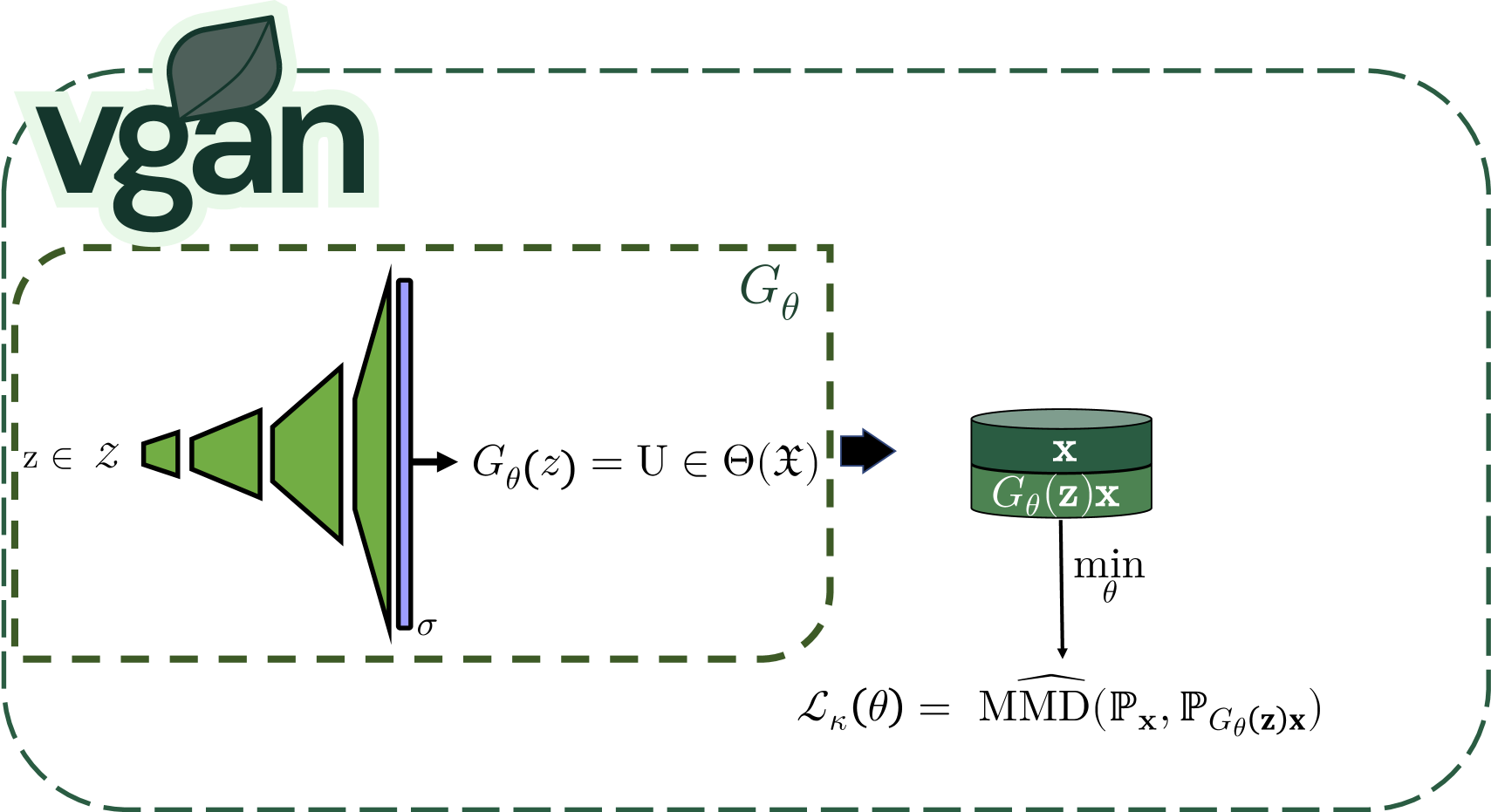
(a) Without kernel learning

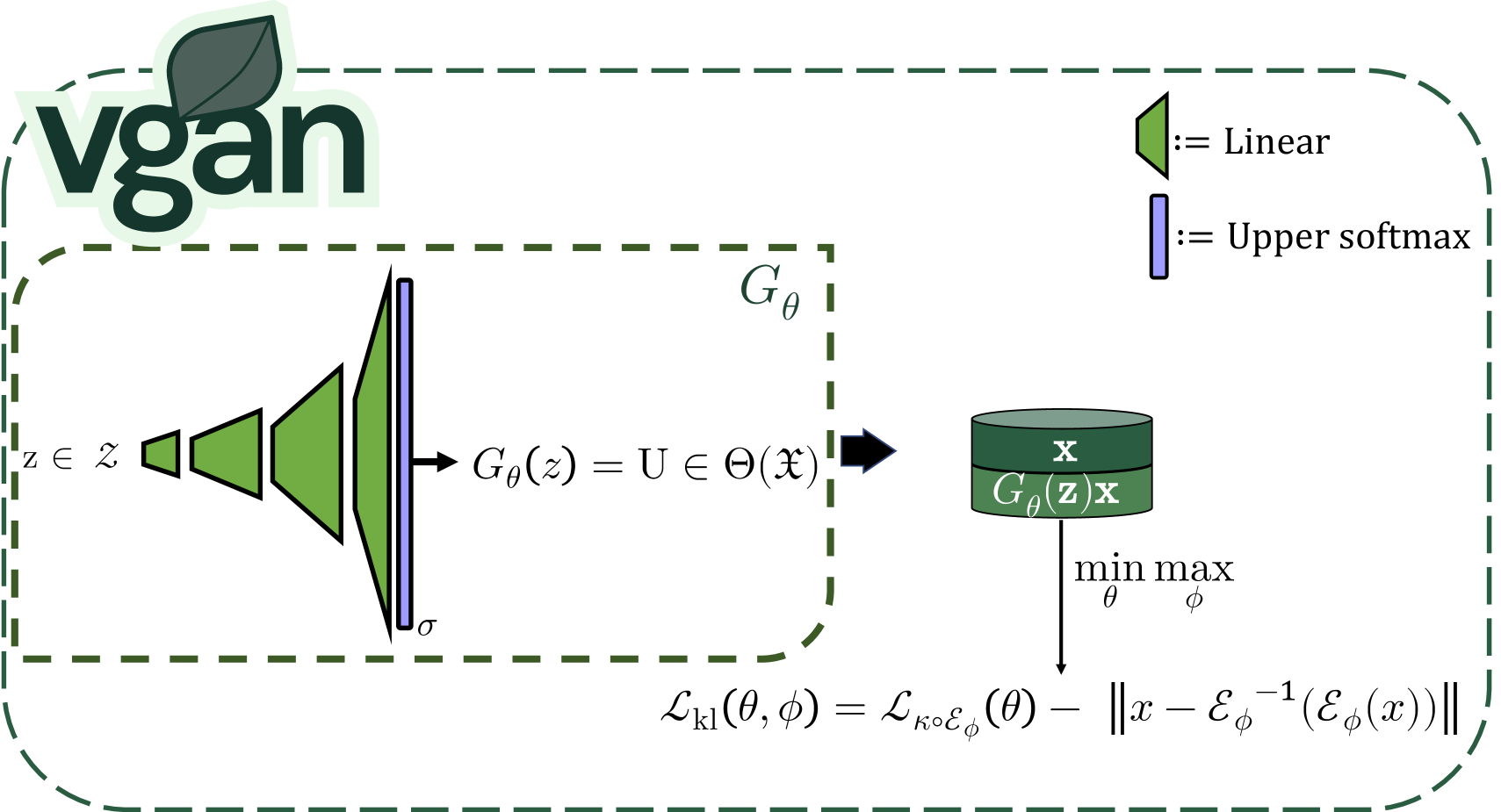
(b) With kernel learning

Figure 2: Diagram of the network and the training without and with kernel learning, from left to right, respectively. (a) The network $G_{\theta}$ is trained to minimize the loss $\mathcal{L}_{\kappa}(\theta)$ — the empirical estimator of the MMD (Gretton et al., 2012) between samples of $\mathbf{x}$ and $G_{\theta}(\mathbf{z})\mathbf{x}$ using kernel $\kappa$. (b) The network $G_{\theta}$ is trained to minimize the same loss as before, but with $\kappa$ composed with $\mathcal{E}_{\phi}$, the encoder part of an autoencoder. At the same time, $\mathcal{E}_{\phi}$ is trained to maximize $\mathcal{L_{\kappa\circ\mathcal{E}_{\phi}}}$, while minimizing the reconstruction loss.

Generator

Figure 2 contains a diagram of the architecture and the training of the generator. It features four hidden linear layers with an increasing number of neurons: $h_{l_{1}}=\frac{d}{8}$, $h_{l_{2}}=\frac{d}{4}$, $h_{l_{3}}=\frac{d}{2}$, and $h_{l_{4}}=d$, where $d$ represents the data dimensionality. The input layer from the latent space has $\frac{d}{16}$ neurons, while the output layer employs the upper softmax activation $\sigma_{\text{us}}$ — see Section 4.

Kernel

Unless stated otherwise, following the advice from (Li et al., 2017), we will use the kernel $\kappa_{\phi}=\varsigma\circ E_{\phi}$. Here, $\varsigma$ is a Gaussian kernel with the median heuristic bandwidth parameter (Garreau et al., 2018) and $E_{\phi}$ an encoder trained by kernel learning — see Section 4.1.2. Particularly, we use an upside-down version of the generator’s hidden layers for $E_{\phi}$, with the identity function as the output layer.

Training

We trainned the network for 2000 epochs, with minibatch gradient descent using the Adadelta optimizer (Zeiler, 2012) following preliminary results. In particular, we use batches of size $500$, a learning rate of $lr_{G}=lr_{E}=0.007$ for the generator and the encoder, respectively. We set momentum ($0.99$) and weight-decay ($0.04$) (Goodfellow et al., 2016). Additionally, we updated $E_{\phi}$ once every 5 epochs.

Number of Subspaces

We generate $500$ samples of the lens operator $\mathbf{V}$ to approximate its distribution. Thus, the number of subspaces depends on the number of unique values of its distribution.

5.1.3 Competitors & Baselines

Table 2: Table of the different competitors in our experiments grouped by method type.

Type	Competitors
Subspace Selection	CLIQUE 2005, HiCS 2012, GMD 2019
Feature Selection	CAE 2019
Embedding Method	PCA 1901, UMAP 2024, ELM 2023

We selected popular and state-of-the-art (SotA) Subspace selection, Feature selection, and Embedding methods with openly available implementations as competitors; see Table 2. For all methods included, we used the recommended parameters and training regimes. Specific details for each competitor are in the appendix, Section B.1. Additionally, we included regular Feature Bagging (FB) (Lazarevic and Kumar, 2005) as a baseline in Section 5.3.1. We built homogeneous feature ensembles using off-the-shelf outlier detectors in the outlier detection experiments. With the Embedding method, we used the embedded version of the dataset to fit a singular off-the-shelf detector. Specifically, we utilized the most popular and best-performing detectors from (Han et al., 2022): LOF, kNN, CBLOF, ECOD, and COPOD (Breunig et al., 2000; Aggarwal, 2017; He et al., 2003; Li et al., 2023; 2020), with their respective recommended or default parameters.

All experiments were implemented in Python. We used popular implementations for all competitors and baselines and implemented $\mathbf{V}$-GAN in PyTorch. We used pyod for outlier detectors, except HiCS, which is in Nim. Experiments ran on a Ryzen 9 7900X CPU and an Nvidia RTX 4090 GPU.

5.2 Obtaining the Theoretical Lens Operator

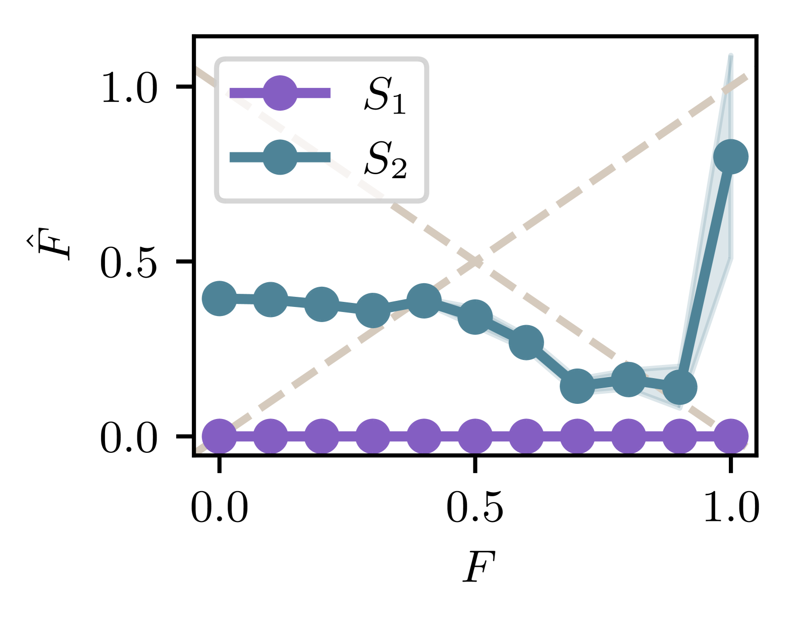
(a) HiCS

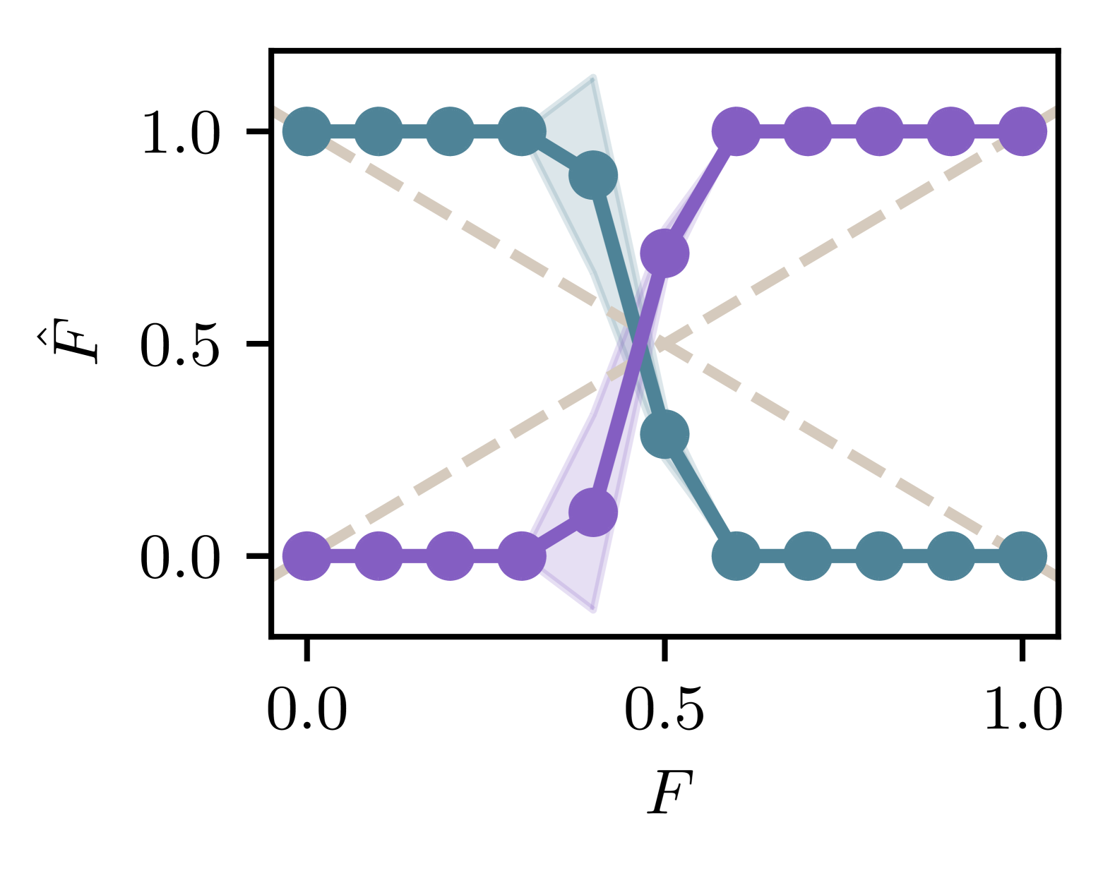
(b) GMD

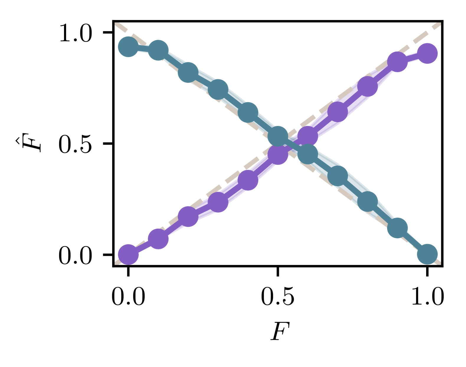
(c) $\mathbf{V}$-GAN

Figure 3: Comparison of the relative scores for each subspace across different values of $F$.

To study the properties of the operator $\mathbf{V}$ obtained by $\mathbf{V}$-GAN, we use synthetic data. Specifically, we consider a population similar to Example 1, where a lens operator can be directly calculated. Using the synthetic population described in Section 5.1.1, we define a random operator $\mathbf{U}$ with values $U_{1}=\text{diag}(1,1,0)$ and $U_{2}=\text{diag}(0,0,1)$, occurring with probabilities $F_{1}=F$ and $F_{2}=1-F$, respectively. This operator is trivially a lens operator. The experiment aims to extract subspaces $S_{1}$ and $S_{2}$ with scores $\hat{F}_{1}$ and $\hat{F}_{2}$ as close as possible to $F_{1}$ and $F_{2}$, using a subspace selection method. The steps are as follows:

1. Generate a dataset $D$ by sampling 10000 points from $\mathbf{x}$.

2. Use $D$ to train a given subspace selection method.

3. Obtain the subspace qualities $\hat{F}_{i}$ of all selected subspaces $\left\{S_{i}\right\}$ and map them into $\left[0,1\right]$ probabilities by $\hat{F}^{\prime}_{i}=\frac{\hat{F}_{i}}{\sum_{j}\hat{F}_{j}}$.

4. Report the probabilties $\hat{F}^{\prime}_{1},\hat{F}^{\prime}_{2}$ of subspaces $S_{1}$ and $S_{2}$.

5. Repeat steps 1$-$4 10 times.

In step 3 we considered the subspace selection methods HiCS and GMD (Keller et al., 2012; Trittenbach and Böhm, 2019) apart from $\mathbf{V}$-GAN. We could not include the subspace selection method CLIQUE (Agrawal et al., 2005) as it does not report a quality metric for the subspaces. As we are using a $3$-dimensional dataset, it will be enough to employ a regular Gaussian kernel with the recommended bandwidth parameter for $\mathbf{V}$-GAN’s training. We reported the results in Figure 3. As we can see, $\mathbf{V}$-GAN is the only method capable of properly extracting the true weight of each subspace.

5.3 One-class Classification

This section presents outlier detection experiments using $\mathbf{V}$-GAN to build ensembles. The goal is to detect outliers in a test set $D^{\text{test}}$ after training on an inlier train set $D^{\text{train}}$, a problem known as one-class classification (Perera et al., 2021). The experimental process is as follows:

1. Split the dataset $D$ into a training set $D^{\text{train}}$ containing $80\%$ of the inliers from $D$, and a test set $D^{\text{test}}$ containing the remaining $20\%$ and the outliers.

2. Obtain a collection of $K$ subspaces $\{S_{i}\}_{i=1}^{K}$ using a susbpace selection method.

3. Given an outlier detector $\mathcal{M}$, obtain $\{\mathcal{M}_{i}\}_{i=1}^{K}$ by fitting $\mathcal{M}$ on each of the $K$ selected subspaces. As a dataset, use $D^{\text{train}}|_{S_{i}}$, the projection of $D^{\text{train}}$ into the subspace.

4. Evaluate the performance of each detector by reporting the AUC of the aggregated scores across all $D^{\text{test}}|_{S_{i}}$. If $K=1$ (like in feature selection), use the score in $D^{\text{test}}|_{S}$.

5. Repeat steps 2 to 4 10 times.

We aim to address two key questions about the performance of $\mathbf{V}$-GAN’s lens operator: (Q1) How does it compare to baselines for outlier detection, such as the full-space method and a randomly selected collection of subspaces (feature bagging)? (Q2) How does it perform relative to other subspace selection methods and dimensionality reduction techniques? Furthermore, we will evaluate its performance on datasets with and without a myopic distribution, providing insights into both the best-case scenario (where $\mathbf{V}$ acts as a lens operator) and the worst-case scenario (where $\mathbf{V}$ does not).

5.3.1 Comparison with Baselines (Q1)

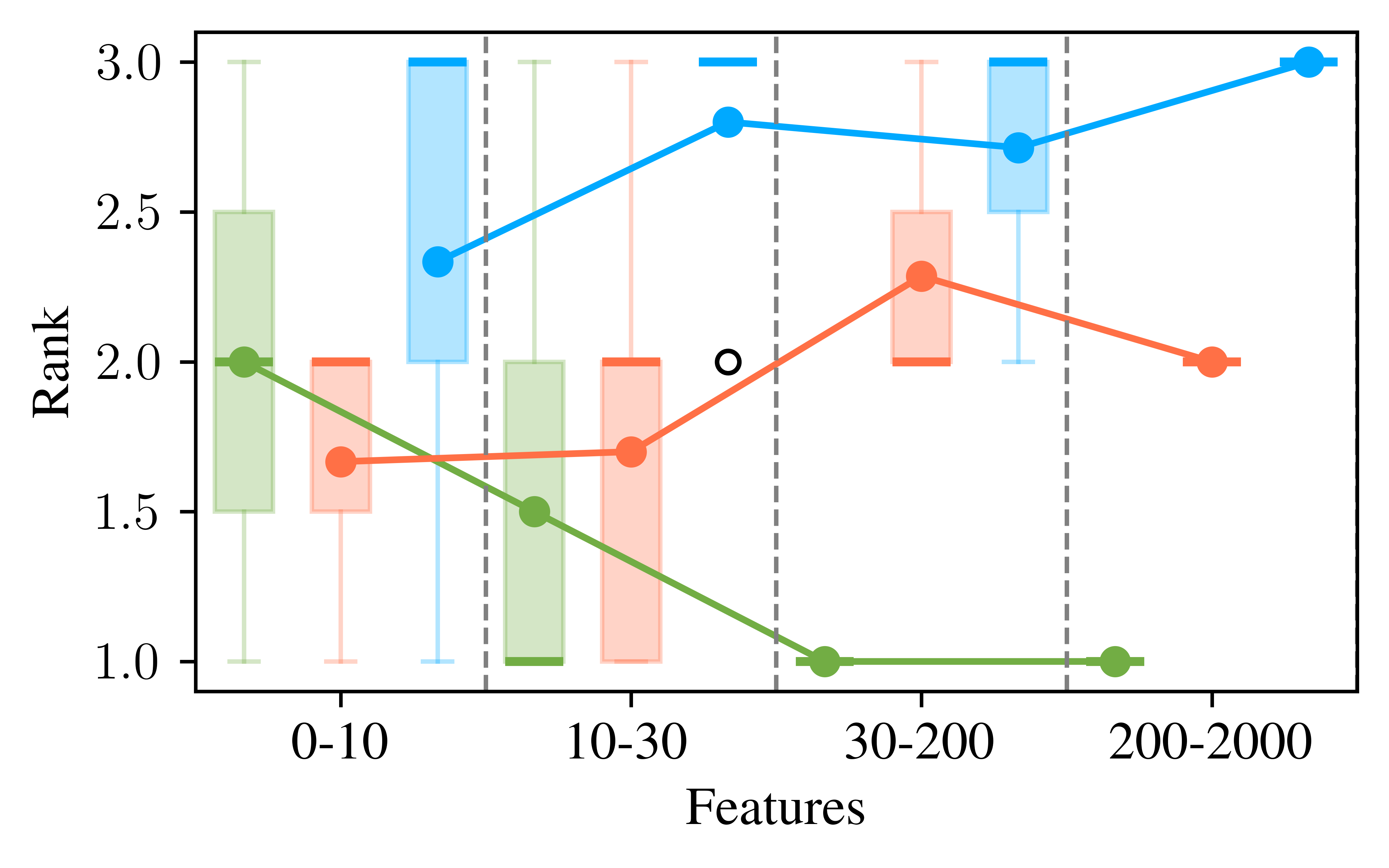
(a) LOF

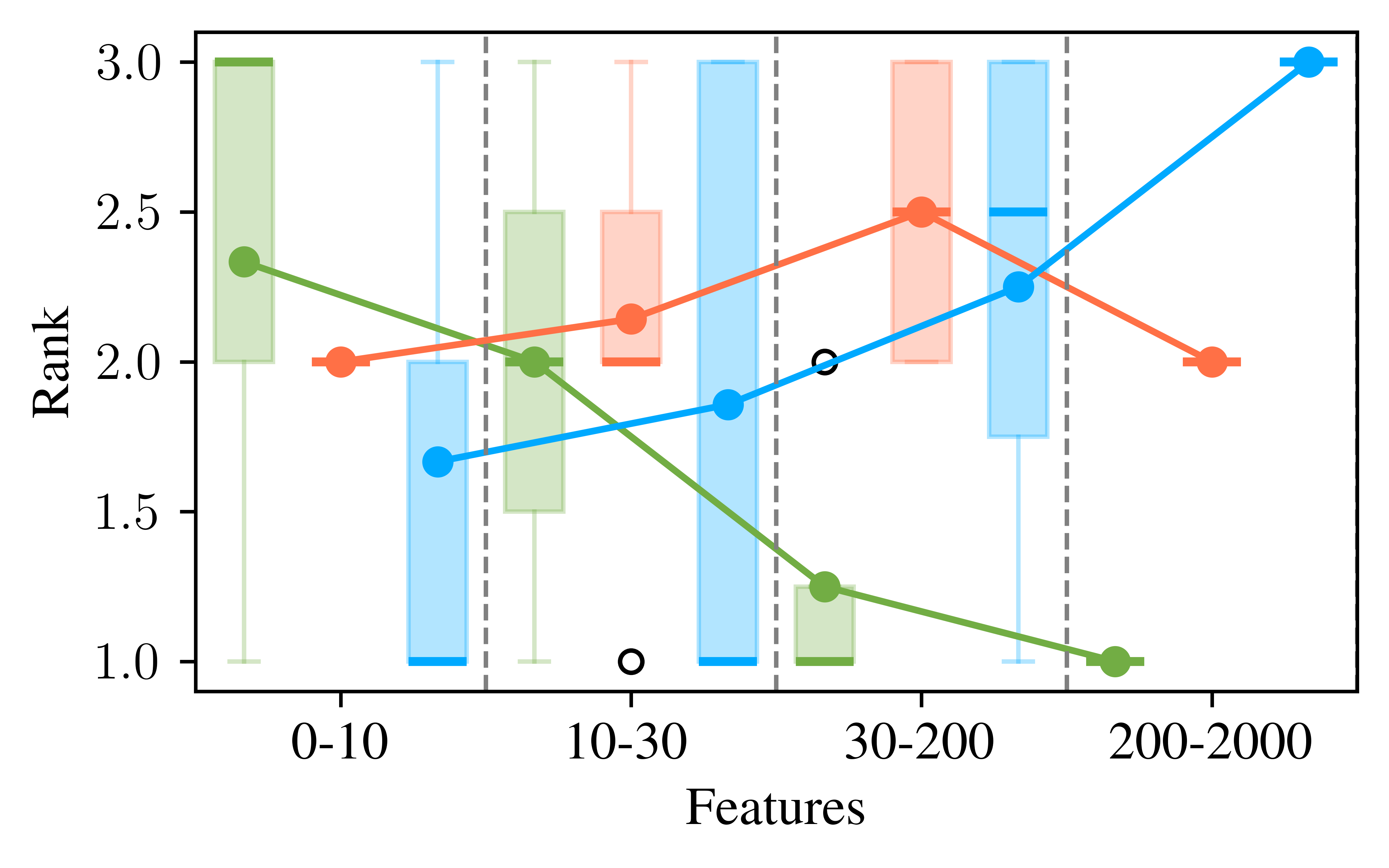
(b) kNN

(c) ECOD

(d) COPOD

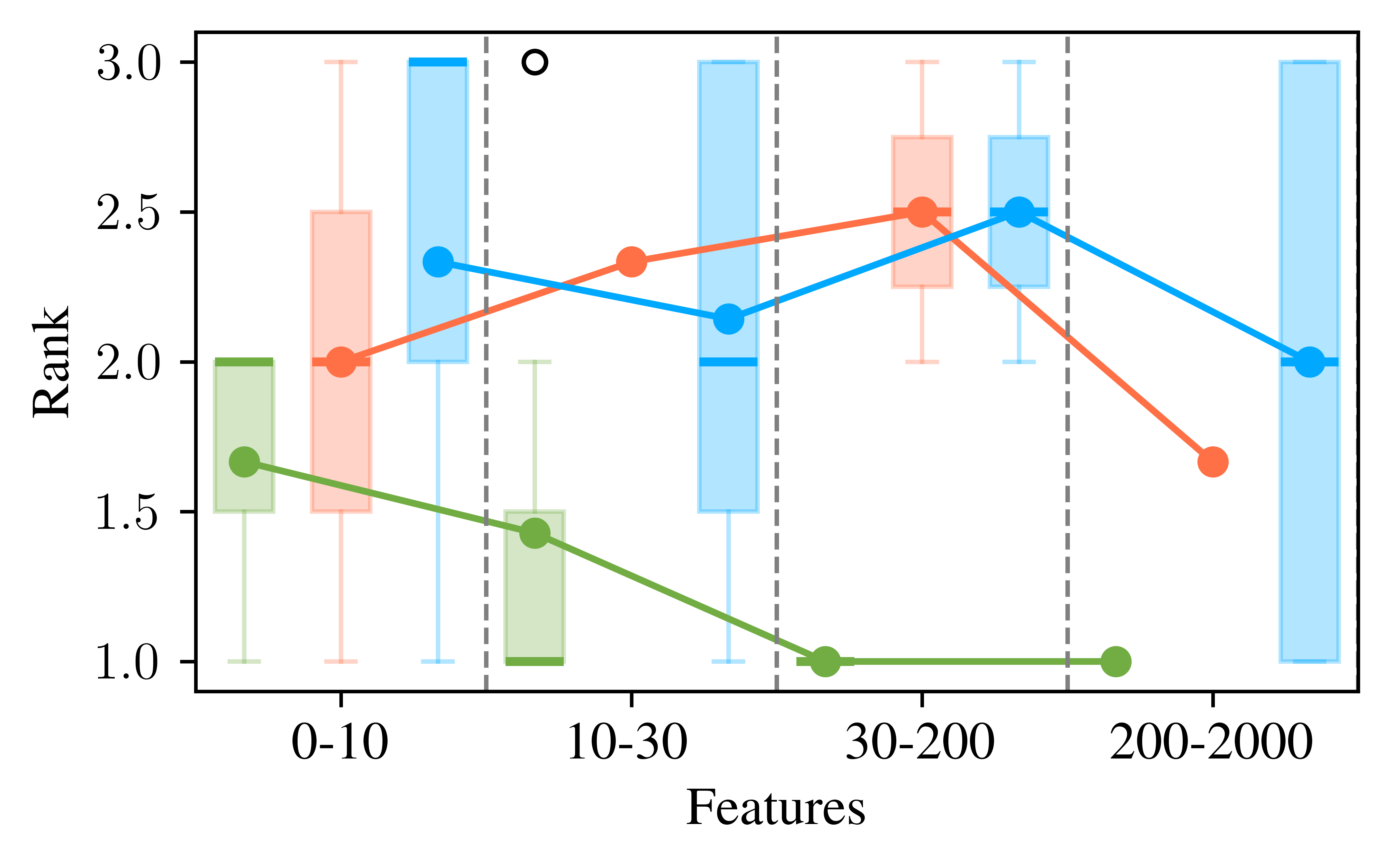
(e) CBLOF

(f) Legend

Figure 4: Boxplots of ranks of the comparison with baselines using myopic datasets with different numbers of features. The bins contained 3, 7, 5, and 6 datasets, respectively.

Table 3: Results of the Conover-Iman test for the rankings against baselines on myopic datasets

	LOF			kNN			ECOD			COPOD			CBLOF
	FB	None	V-GAN	FB	None	V-GAN	FB	None	V-GAN	FB	None	V-GAN	FB	None	V-GAN
FB		+ +	- -			- -			- -			- -			- -
None	- -		- -			- -			- -			- -	- -
V-GAN	+ +	+ +		+ +	+ +		+ +	+ +		+ +	+ +		+ +	+ +

In this section, we compare $\mathbf{V}$-GAN to two classical baselines in the subspace selection literature: the full-space method and Feature Bagging (FB) (Lazarevic and Kumar, 2005). For FB, we chose the number of subspaces $K$ from a set of five equidistant values from $50$ to $500$. For each dataset, we selected the $K$ yielding the highest average AUC across 10 repetitions. To aggregate scores, we used a weighted average based on the probability assigned to each subspace, following (Cribeiro-Ramallo et al., 2024, Propositon 1). For FB, this reduces to a simple average.

Furthermore, we will evaluate its performance on datasets with and without a myopic distribution, providing insights into both the best-case scenario (where $\mathbf{V}$ is a lens operator) and the worst-case scenario (where $\mathbf{V}$ is not). To study whether this is the case for each dataset, we will study the hypothesis test presented in Section 4.2. We collected the test results in Tables 7-11. Further details can be found in Section B.1 in the Appendix.

Myopic Datasets.

Figure 4 shows rankings contingent on dataset dimensionality group and average rankings. $\mathbf{V}$-GAN demonstrates consistent performance improvements as dimensionality increases, often outperforming baselines for all outlier detectors. To assess statistical significance, we apply the Conover-Iman post-hoc test (Conover and Iman, 1979), commonly used in outlier detection (Campos et al., 2016), following a preliminary positive result from the Kruskal-Wallis test (Kruskal and Wallis, 1952). Table 3 contains the results, where ‘$+$’ indicates the row method has a significantly lower median rank than the column method, and ‘$-$’ indicates a significantly higher rank. One symbol marks p-values $\leq 0.1$, two symbols mark p-values $\leq 0.05$, and blanks indicate no significant difference. Entirely grayed-out subtables denote cases where the Kruskal-Wallis test, a prerequisite for using the Conover-Iman post-hoc test, was not passed. $\mathbf{V}$-GAN outperformed all baselines across detectors. The appendix summarizes the complete AUC results in Tables 7-11.

Non-myopic Datasets.

Non-myopicity represents the worst-case scenario for $\mathbf{V}$-GAN, as its guarantees rely on this property. Figure 7 in the Appendix shows rank boxplots for non-myopic datasets, similar to those for myopic datasets. It is evident that $\mathbf{V}$-GAN’s performance is not worse than any baseline, and the Conover-Iman test results (Table 5) support this. $\mathbf{V}$-GAN’s performance in its worst-case scenario is no worse than that of a tuned feature bagging (FB) and outperforms the full-space approach for some outlier detectors.

5.3.2 Comparison with Competitors (Q2)

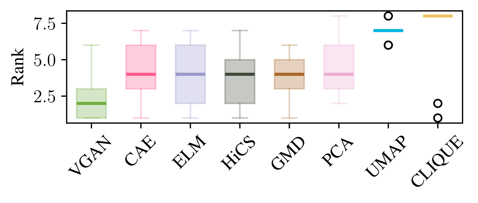
(a) LOF

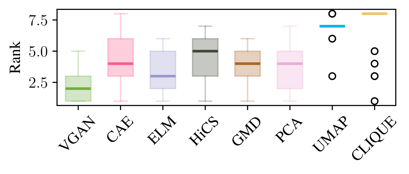
(b) kNN

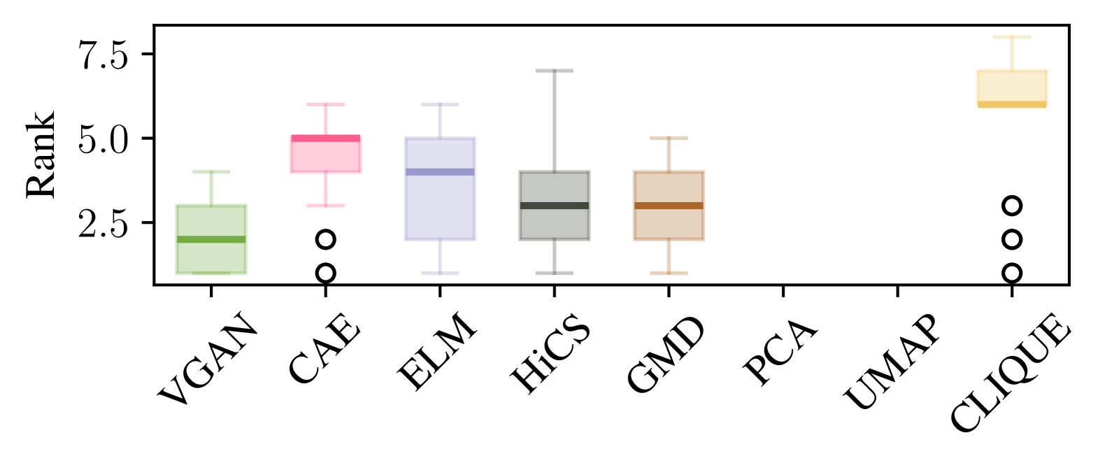
(c) ECOD

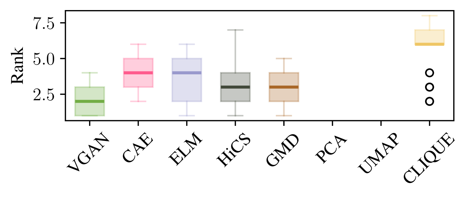
(d) COPOD

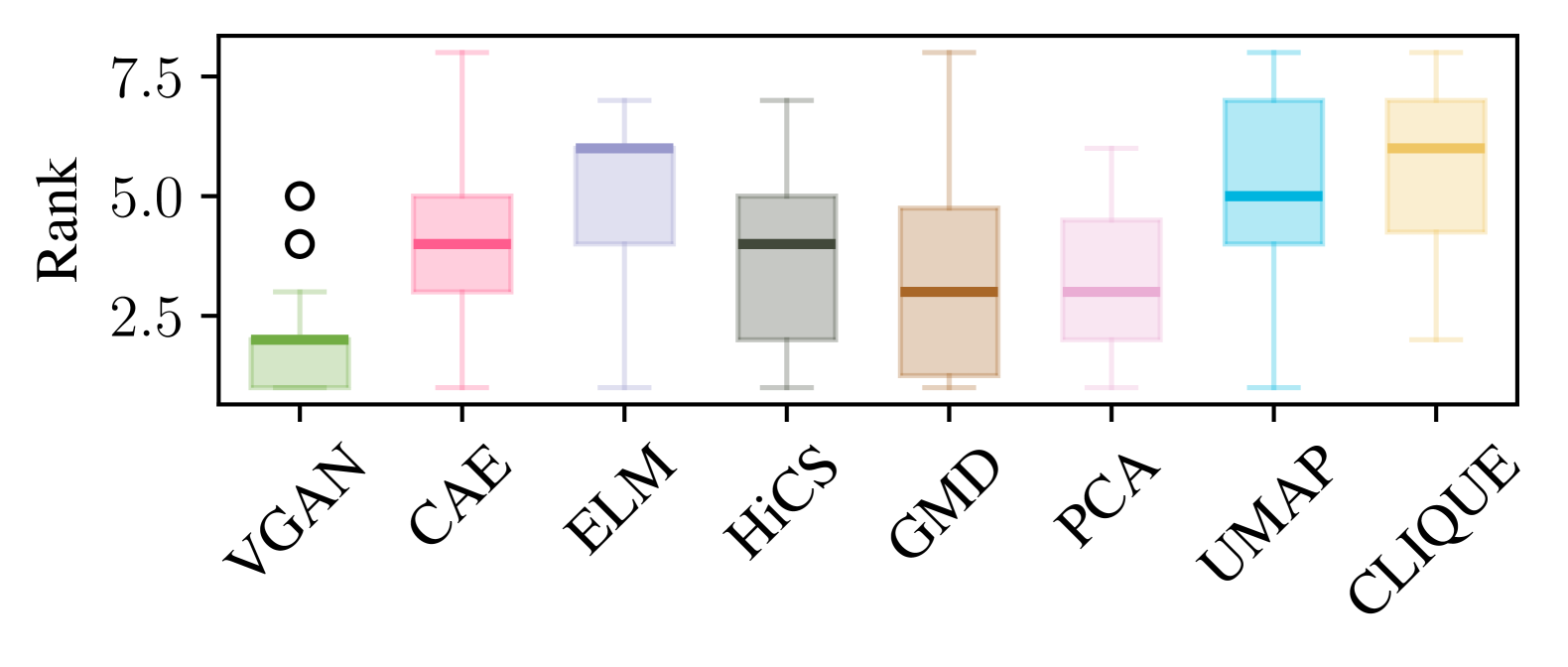
(e) CBLOF

Figure 5: Boxplots of ranks of the comparison with our competitors using myopic datasets.

We now compare $\mathbf{V}$-GAN to the competitors introduced in Section 5.1.3 (see Table 1). As before, we analyze performance separately for myopic and non-myopic datasets.

Myopic Datasets.

Figure 5 plots the ranks of all competitors for myopic datasets. $\mathbf{V}$-GANconsistently achieves the lowest median rank, with GMD typically being the closest competitor. Table 4 contains the results of the Conover-Iman test. $\mathbf{V}$-GAN significantly outperforms all methods and is the best option for enhancing outlier detection performance under myopicity.

Non-myopic Datasets.

Figure 8 plots ranks for the non-myopic case, and Table 6 contains the Conover-Iman test results. $\mathbf{V}$-GAN demonstrates a closer performance to its competitors on non-myopic datasets, as expected, but it is never statistically worse than any competitor. I.e., we can recommend $\mathbf{V}$-GAN as a default approach for ensemble outlier detection using subspaces, which brings significant advantages in the myopic case while having no disadvantage in the absence of myopicity.

Table 4: Results of the Conover-Iman test for the rankings against competitors on myopic datasets

OD method	SS method	CAE	HiCS	CLIQUE	ELM	GMD	PCA	UMAP	V-GAN
LOF	CAE			$++$				$++$	$--$
	HiCS			$++$				$++$	$--$
	CLIQUE	$--$	$--$		$--$	$--$	$--$		$--$
	ELM			$++$				$++$	$--$
	GMD			$++$				$++$	$--$
	PCA			$++$				$++$	$--$
	UMAP	$--$	$--$		$--$	$--$	$--$		$--$
	V-GAN	$++$	$++$	$++$	$++$	$++$	$++$	$++$
kNN	CAE			$++$	$--$		$+$	$++$	$--$
	HiCS			$++$	$+$			$++$	$--$
	CLIQUE	$--$	$--$		$--$	$--$	$--$		$--$
	ELM	$++$	$-$	$++$				$++$	$--$
	GMD			$++$				$++$	$--$
	PCA	$-$		$++$				$++$	$--$
	UMAP	$--$	$--$		$--$	$--$	$--$		$--$
	V-GAN	$++$	$++$	$++$	$++$	$++$	$++$	$++$
ECOD	CAE		$--$	$++$	$+$	$--$			$--$
	HiCS	$++$		$++$					$--$
	CLIQUE	$--$	$--$		$--$	$--$			$--$
	ELM	$-$		$++$					$--$
	GMD	$++$		$++$					$--$
	PCA
	UMAP
	V-GAN	$++$	$++$	$++$	$++$	$++$
COPOD	CAE		$--$	$++$		$--$			$--$
	HiCS	$++$		$++$					$--$
	CLIQUE	$--$	$--$		$--$	$--$			$--$
	ELM			$++$					$--$
	GMD	$++$		$++$					$-$
	PCA
	UMAP
	V-GAN	$++$	$++$	$++$	$++$	$+$
CBLOF	CAE			$++$					$--$
	HiCS			$++$	$++$			$++$	$--$
	CLIQUE	$--$	$--$			$--$	$--$		$--$
	ELM		$--$			$--$	$--$		$--$
	GMD			$++$	$++$			$++$	$-$
	PCA			$++$	$++$			$++$	$--$
	UMAP		$--$			$--$	$--$		$--$
	V-GAN	$++$	$++$	$++$	$++$	$+$	$++$	$++$

5.4 Scalability

We now compare the scalability of $\mathbf{V}$-GAN with other subspace search methods. For these experiments, all methods were tested with their parameters set as in Section 5.1.2. The dataset consists of uniformly generated noise with $d\in\{0.1,1.2,2.3,3.4,4.5,5.6,6.7,7.8,8.9,10\}\cdot 10^{3}$ features. All experiments are run using a single CPU thread to ensure a fair comparison.

Figure 6 presents the results of scalability experiments, showing the runtime in hours required to obtain a collection of subspaces as a function of the number of features. $\mathbf{V}$-GAN is more scalable than all subspace search competitors: It is over 4, 30, and 8000 times faster than HiCS, GMD, and CLIQUE, respectively.

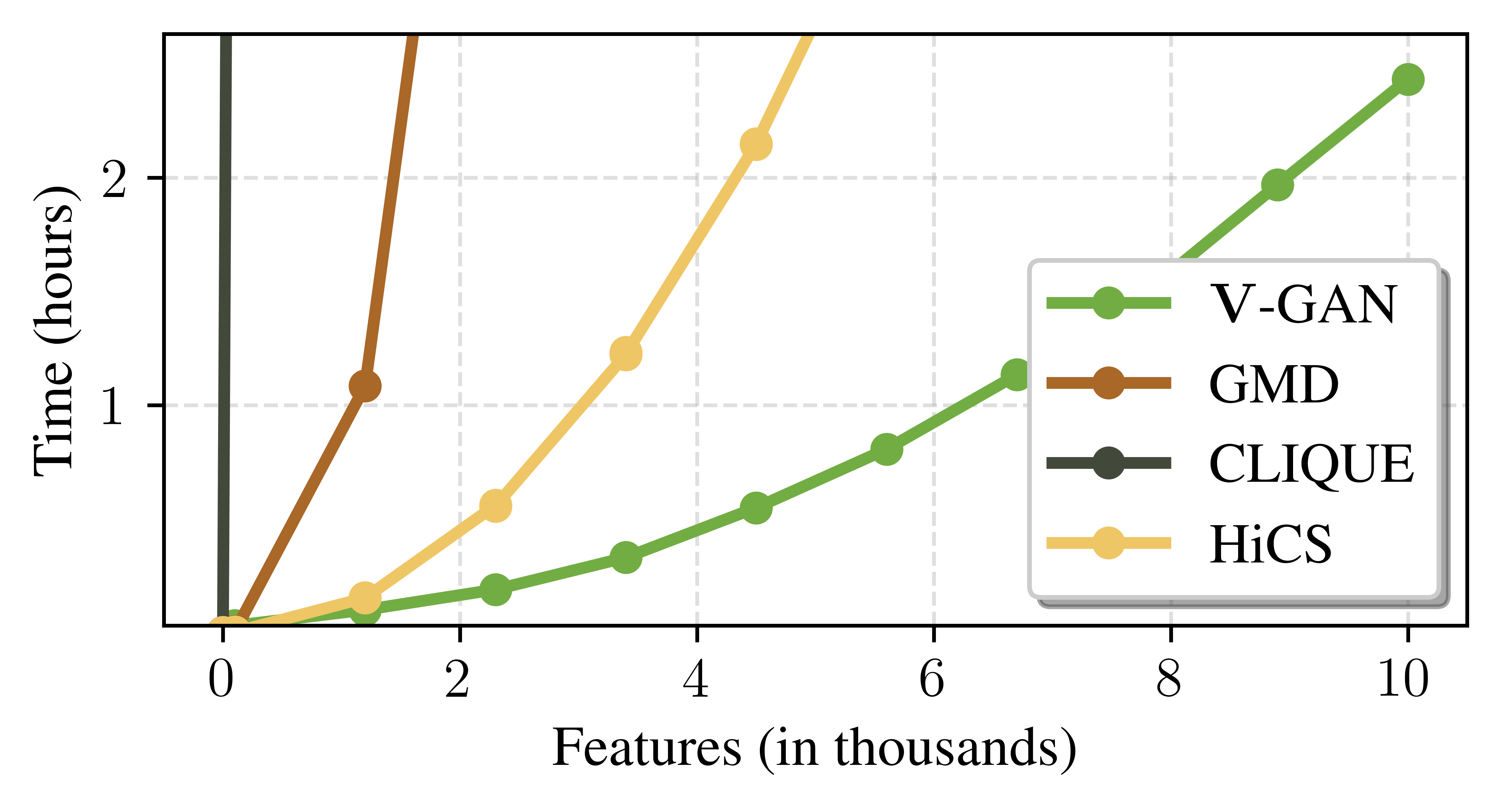
Figure 6: Time taken for performing subspace search, per feature count.

6 Conclusions & Future Work

Subspace search can improve outlier detection for an off-the-shelf detector in tabular data (Müller et al., 2012; Keller et al., 2012; Nguyen et al., 2014; Trittenbach and Böhm, 2019). In our experiments, however, we did not observe this improvement in all datasets, with the methods sometimes failing to beat näive baselines. Besides, existing subspace search methods can hardly be applied to non-tabular data due to poor scaling. The abovementioned factors hindered the use of such methods in practice. This paper proposes a new theoretical framework that explains when subspace selection is helpful and, more importantly, how can we exploit it in our advantage. Using this theory, we introduced a new way of performing subspace selection, akin to subspace search methods, that is theoretically sound, scalable and usable in general scenarios — a strategy that we called subspace generation. Our first attempt in subspace generation, called $\mathbf{V}$-GAN, demonstrate a significant performance increase againts other baselines and competitors in the downstream task of outlier detection — one of the main use cases for subspace search. In addition, our experiments suggest that the performance increase is conditioned on the data’s distribution being myopic, a property we can infere from data without any prior knowledge. Furthermore, even when the data is not myopic, $\mathbf{V}$-GAN is still not outperformed by its competitors.

Our findings not only validate the superior performance of $\mathbf{V}$-GAN for subspace selection, but also show the potential of our Myopic Subspace Theory (MST) beyond the use case of outlier detection on tabular data. Thus, our most important future work is to assess whether MST can be useful with other datatypes, beyond the preliminary experiments in Section B.2. Furthermore, as the operators introduced in MST are not limited to projections, other machine learning problems might benefit from it. One example is constrastive learning, which relies on creating diverse augmentations or views of the data to learn invariant features (Chen et al., 2020). A set of realizations from a lens operator are transformations that preserve the underlying data distribution, which could act as semantically meaningful "views" for contrastive pairs.

Aknowledgements

This work was supported by the Ministry of Science, Research and the Arts Baden-Württemberg, project Algorithm Engineering for the Scalability Challenge (AESC).

Appendix A Theoretical Appendix

This appendix contains the proofs for all the statements in Section 3, extra general statements, and a collection of examples of lens operators on different spaces.

A.1 Myopic Subspace Theory (Extension)

We will first introduce all of the proofs of the statemes from Section 3, and then introduce all of the additional statements and proofs. To maintain the clarity of this section, we will re-introduce all of the statements before their proofs.

Lemma 1.

Consider $\mathcal{H}$ a RKHS with a characteristic kernel $\kappa$; and $\mathbf{x}$, $\mathbf{U}$ and MMD as previously defined. Further, consider $\mathbf{V}$ to be a lens operator for $\mathbf{x}$. Then,

$$\underset{\mathbf{U}}{\arg\min}\emph{\text{MMD}}_{\kappa}(\mathbb{P}_{\mathbf{x}},\mathbb{P_{\mathbf{Ux}}})\ni\mathbf{V}$$

Proof.

$\mathbf{V}$ lens for $\mathbf{x}\Longrightarrow$ $\mathbb{P}_{\mathbf{Vx}}=\mathbb{P}_{\mathbf{x}}\Longrightarrow\text{MMD}_{\kappa}(\mathbb{P}_{\mathbf{Vx}},\mathbb{P}_{\mathbf{x}})=0\Longrightarrow\mathbf{V}\in\underset{\mathbf{U}}{\arg\min}\text{MMD}(\mathbb{P}_{\mathbf{x}},\mathbb{P}_{\mathbf{Vx}})$. The first implication comes from the definition of a lens operator, the second for $\kappa$ being characteristic, and the last one is trivial when considering $\text{MMD}_{\kappa}(\mathfrak{p},\mathfrak{q})\geq 0,~\forall\mathfrak{p,q}\in\mathcal{M}_{1}^{+}$. ∎

Theorem 2.

Consider $\mathbf{x}$ a random variable on $(E,\mathcal{T})$ — a separable metric space — and $\mathbf{U}$ a random operator taking values on $\Theta(\mathfrak{X})\subset\mathcal{C}(\mathfrak{X})$. Further consider the associated RKHS $\mathcal{H}$ of functions on $E$ with characteristic kernel $\kappa$, the induced MMD metric on $\mathcal{M}_{1}^{+}$. Under these conditions, if $\mathcal{M}_{\mathbf{x}}^{{\Theta(\mathfrak{X})}}$ is compact and $\mathbf{x}$ $\Theta(\mathfrak{X})$-myopic, we have that:

1. Given an iterative convergence strategy $\mathfrak{F}$ such that $\mathfrak{F}(\mathfrak{p}_{n-1})=\mathfrak{p}_{n}\in\mathcal{N}\subset\mathcal{M}_{1}^{+}$ and $\{\mathfrak{p}_{n}\}_{n\in\mathbb{N}}\longrightarrow\mathfrak{p}^{\prime}\in\underset{\mathfrak{p}\in\mathcal{N}}{\arg\inf}\text{ \emph{MMD}}_{\kappa}(\mathbb{P}_{\mathbf{x}},\mathfrak{p})$, it follows that:

   $$\mathfrak{F}(\mathfrak{p}_{n-1})=\mathfrak{p}_{n}\in\mathcal{M}_{\mathbf{x}}^{\Theta(\mathfrak{X})}\Longrightarrow\{\mathfrak{p_{n}}\}_{n\in\mathbb{N}}\longrightarrow\mathfrak{p}^{\prime}\in\underset{\mathfrak{p}\in\mathcal{M}_{1}^{+}}{\arg\min}\text{ \emph{MMD}}_{\kappa}(\mathbb{P}_{\mathbf{x}},\mathfrak{p})\text{ and }\mathfrak{p}^{\prime}\in\mathcal{M}_{\mathbf{x}}^{\Theta(\mathfrak{X})}.$$

Proof.

By the definition of $\mathfrak{F}$, we can construct a sequence $\{\mathfrak{p}_{n}\}_{n\in\mathbb{N}}\in\mathcal{M}_{\mathbf{x}}^{\Theta(\mathfrak{X})}$ such that

$$\{\mathfrak{p}_{n}\}_{n\in\mathbb{N}}\longrightarrow\mathfrak{p}^{\prime}\in\underset{\mathfrak{p}\in\mathcal{M}_{\mathbf{x}}^{\Theta(\mathfrak{X})}}{\arg\min}\text{MMD}_{\kappa}(\mathbb{P}_{\mathbf{x}},\mathfrak{p})$$ (11)

Since $\mathbf{x}$ is $\Theta(\mathfrak{X})-$myopic, $\exists\mathbf{V}:\Omega\longrightarrow\Theta(\mathfrak{X})$ that is a lens operator for $\mathbf{x}$. By Lemma 1, and the definion of $\mathcal{M}_{\mathbf{x}}^{\Theta(\mathfrak{X})}$, is clear that:

$$\mathbb{P}_{\mathbf{Vx}}\in\underset{\mathfrak{p}\in\mathcal{M}_{\mathbf{x}}^{\Theta(\mathfrak{X})}}{\arg\min}\text{MMD}_{\kappa}(\mathbb{P}_{\mathbf{x}},\mathfrak{p}).$$ (12)

Additionally, by the definition of a lens operator,

$$\mathbb{P}_{\mathbf{Vx}}\in\underset{\mathfrak{p}\in\mathcal{M}_{1}^{+}}{\arg\min}\text{MMD}_{\kappa}(\mathbb{P}_{\mathbf{x}},\mathfrak{p}).$$ (13)

Thus, by (11), (12), and (13), is clear that

$$\mathfrak{p}^{\prime}\in\underset{\mathfrak{p}\in\mathcal{M}_{1}^{+}}{\arg\min}\text{MMD}_{\kappa}(\mathbb{P}_{\mathbf{x}},\mathfrak{p}).$$

Additionally, as $\{\mathfrak{p}_{n}\}_{n\in\mathbb{N}}$ is a sequence in a compact space,

$$\{\mathfrak{p}_{n}\}_{n\in\mathbb{N}}\longrightarrow\mathfrak{p}^{\prime}\in\mathcal{M}_{\mathbf{x}}^{\Theta(\mathfrak{X})}.$$

∎

Corollary 3 (Convergence to a myopic operator).

Consider $\mathbf{x}$ a random variable on $(E,\mathcal{T})$ — a separable metric space — and $\mathbf{U}$ a continous random operator taking values on $\Theta(\mathfrak{X})\subset\mathcal{C}(\mathfrak{X})$. Further consider the associated RKHS $\mathcal{H}$ of functions on $E$ with characteristic kernel $\kappa$ and the induced MMD metric on $\mathcal{M}_{1}^{+}$. Under this conditions, if $\Theta(\mathfrak{X})$ is compact and $\mathbf{x}$ is $\Theta(\mathfrak{X})$-myopic, we have that

1. Given an iterative convergence strategy $\mathfrak{F}$ such that $\mathfrak{F}(\mathfrak{p}_{n-1})=\mathfrak{p}_{n}\in\mathcal{N}\subset\mathcal{M}_{1}^{+}$ and $\{\mathfrak{p}_{n}\}_{n\in\mathbb{N}}\longrightarrow\mathfrak{p}^{\prime}\in\underset{\mathfrak{p}\in\mathcal{N}}{\arg\inf}\text{ \emph{MMD}}_{\kappa}(\mathbb{P}_{\mathbf{x}},\mathfrak{p})$, it follows that:

   $$\{\mathbf{U}_{n}\}_{n\in\mathbb{N}}\text{ such that }\mathfrak{F}(\mathbb{P}_{\mathbf{U}_{n-1}\mathbf{x}})=\mathbb{P}_{\mathbf{U}_{n}\mathbf{x}}\Longrightarrow\text{\emph{MMD}}_{\kappa}(\mathbb{P}_{\mathbf{x}},\mathbb{P}_{\mathbf{U}_{n}\mathbf{x}})\longrightarrow 0,\text{ and }\{\mathbf{U}_{n}\}_{n\in\mathbb{N}}\longrightarrow\mathbf{V}\in\Theta(\mathfrak{X}).$$

Proof.

Consider $\{\mathfrak{p}_{n}\}_{n\in\mathbb{N}}\in\mathcal{M}_{\mathbf{x}}^{\Theta(\mathfrak{X})}$, such that $\mathfrak{F}(\mathfrak{p}_{n-1})=\mathfrak{p}_{n}.$ By Zorn’s Lemma, one can construct a parallel sequence $\{\mathbf{U}_{n}\}_{n\in\mathbb{N}}$ such that $\mathfrak{F}(\mathfrak{p}_{n-1})=\mathfrak{p}_{n}=\mathbb{P}_{\mathbf{U}_{n}\mathbf{x}}.$ As such,

$$\{\mathbb{P}_{\mathbf{U}_{n}\mathbf{x}}\}\longrightarrow\mathfrak{p}^{\prime}\in\underset{\mathfrak{p}\in\mathcal{M}_{\mathbf{x}}^{\Theta(\mathfrak{X})}}{\arg\inf}\text{MMD}(\mathbb{P}_{\mathbf{x}},\mathfrak{p}).$$

If $\mathcal{M}_{\mathbf{x}}^{\Theta(\mathfrak{X})}$ is compact, we can solve the remainder of the proof equivalently as done for Theorem 2. Thus, we will focus on proving such a statement.

$\Theta(\mathfrak{X})$ compact $\Longrightarrow$ $\{U_{n}\}_{n\in\mathbb{N}}\longrightarrow V$ for all sequences in $\Theta(\mathfrak{X})$. If we now consider $\{\mathbf{U}_{n}\}_{n\in\mathbb{N}}$ and $\mathbf{V}$ such that $\mathbf{U}_{n}(\omega)=U_{n}\longrightarrow V=\mathbf{V}(\omega)$ for almost all $\omega\in\Omega$, it is clear that:

$$\mathbb{P}(\lim_{n}\mathbf{U}_{n}(\omega)=\mathbf{V}(\omega))=1.$$

In other words, $\mathbf{U}_{n}\overset{a.s}{\longrightarrow}\mathbf{V}$. Therefore, since $\Theta(\mathfrak{X})\subset\mathcal{C}(\mathfrak{X})$ and $E$ is a separabale metric space, by the definition of almost sure convergence it is clear that:

$$\mathbf{U}_{n}\overset{a.s}{\longrightarrow}\mathbf{V}\Longrightarrow\mathbf{U}_{n}\mathbf{x}\overset{a.s}{\longrightarrow}\mathbf{Vx}.$$

And lastly, by the convergence laws of random variables, we know that:

$$\mathbf{U}_{n}\mathbf{x}\overset{a.s}{\longrightarrow}\mathbf{Vx}\Longrightarrow\mathbf{U}_{n}\mathbf{x}\overset{d}{\longrightarrow}\mathbf{Vx}\Longrightarrow\mathbb{P}_{\mathbf{U}_{n}\mathbf{x}}\longrightarrow\mathbb{P}_{\mathbf{Vx}}.$$

∎

Now, we introduce the result mentioned at the end of Section 3.3. This result motivates the way we aggregate in our outlier detection experiments.

Proposition 4.

Consider $E$ a Radon space, $(\Omega,\mathcal{F},\mathbb{P})$ a probability space, $\mathfrak{X}$ the space of random variables on $E$, and $\Theta(\mathfrak{X})$ the space of operators from $\mathfrak{X}$ to $\mathfrak{X}$. Further consider all $U\in\Theta(\mathfrak{X})$ to be defined on fibers of $E$, and $\mathbf{U}:\Omega\longrightarrow\Theta(\mathfrak{X})\subset\mathcal{C}(\mathfrak{X})$ a lens operator for $\mathbf{x}\in\mathfrak{X}$. Lastly, consider the following conditions

• $\mathbf{U}$ is such that, given any two realizations $U_{1}$ and $U_{2}$ ($U_{1}\neq U_{2}$), if $\mathbb{P}_{U_{1}\mathbf{x}}(A)\neq 0\Longrightarrow\mathbb{P}_{U_{2}\mathbf{x}}(A)=0,$ for $A\in\mathcal{F}(\mathbf{Ux})$ — i.e., all realizations are mutually exclusive.

• The set of all realizations of $\mathbf{U}$ is countable.

• There exists a meassure $\mu$ such that $\mu>>\mathbb{P}_{\mathbf{Ux}}$ and $\mu>>\mathbb{P}_{\mathbf{U}(\omega)\mathbf{x}}$, $\forall\omega\in\Omega.$

In this case, $\mathbb{P}_{\mathbf{x}}=\sum_{\omega\in\Omega}\mathbb{P}_{\mathbf{U}}(\mathbf{U}(\omega))\mathbb{P}_{\mathbf{U}(\omega)\mathbf{x}}$ and $P_{\mathbf{x}}=\sum_{\omega\in\Omega}\mathbb{P}_{\mathbf{U}}(\mathbf{U}(\omega))P_{\mathbf{U}(\omega)\mathbf{x}}$.

Proof.

Consider all $U\in\Theta(\mathfrak{X})$ to be defined on fibers of $E$. By the disintegration theorem, we know that the pushforward functions $U_{*}\mathbb{P}_{\mathbf{x}}$ are (probability) measures. Then, by $(i)-(ii)$, we can apply the law of total probabilities to derive:

$$\mathbb{P}_{\mathbf{Ux}}=\sum_{\omega\in\Omega}\mathbb{P}_{\mathbf{U}}(\mathbf{U}(\omega))\mathbb{P}_{\mathbf{U}(\omega)\mathbf{x}}.$$

The result for the densities (in the Radon-Nikodym sense) is imediate by the Radon-Nikodym Theorem. ∎

These conditions are trivially fulfilled by the axis-parallel case for outlier detection — akin to the one in [Cribeiro-Ramallo et al., 2024, Proposition 1]. Consider that this result focuses on the case when the operators $U\in\Theta(\mathfrak{X})$ each reside on different fibers of the space $E$, which is enough for our downstream setting.

Coming next, we will introduce a collection of examples of lens operators for a different set of cases — not necessarily having $\Theta(\mathfrak{X})$ defined on fibers of $E$.

Example 2.

• Normal Projected Population from Example 1. Consider the same population as Example 1, with $F=0.5$. Clearly, by the law of total probabilities

  $$\mathbb{P}_{\mathbf{x}}=\frac{1}{2}\mathbb{P}_{\mathbf{x|x\in}S_{1}}+\frac{1}{2}\mathbb{P}_{\mathbf{x|x\in}S_{2}}.$$

  In this case, any non-zero measurable set on $S_{1}$ will get projected into a zero-measure set in $S_{2}$, and vice-versa. Thus, we can write $\mathbb{P}_{\mathbf{x|x\in}S_{1}}=\mathbb{P}_{U_{1}\mathbf{x}}$ and $\mathbb{P}_{\mathbf{x|x\in}S_{2}}=\mathbb{P}_{U_{2}\mathbf{x}}$, with

  $$U_{1}=\begin{pmatrix}1&0&0\\ 0&1&0\\ 0&0&0\end{pmatrix},~U_{2}=\begin{pmatrix}0&0&0\\ 0&0&0\\ 0&0&1\end{pmatrix}.$$

  Equivalently, defining $\mathbf{U}$ as randomly taking values on $\{U_{1},U_{2}\}$ with equal probability trivially fulfills the conditions of Proposition 4.

• Homoskedastic errors. Assume the following random variable $\mathbf{y}=\beta\mathbf{x}+\varepsilon$, with $\beta\in\mathbb{R}^{d\times d}$ and $\varepsilon$ another random variable acting as noise. Now, given an infinite set $D=\{\beta x_{i}+\varepsilon_{i}\}_{i\in I}$ of samples of $\mathbf{y}$, we can define

  $$U_{i}:\beta x_{j}+\varepsilon_{j}\in\mathbb{R}^{d}\longmapsto\beta x_{j}+\varepsilon_{i}\in\mathbb{R}^{d},~\forall i\in I.$$

  As such, defining a $\mathbf{U}$ selecting all $U_{i}$ with equal probability will trivially be a lens operator, if all $\varepsilon_{i}$ are equally distributed. The finite sample setting of this case is a common bootstrap technique known as Resampling Residuals.

• Location Operator for the Variance. A trivial example in $\mathbb{R}$ can be obtained by considering the random variables $\mathbf{x}\sim\mathbb{P}_{\mathbf{x}}$ and $\mathbf{y}=Var(\mathbf{x}).$ Consider $\mathbf{U}(\omega)\in\{U_{1},U_{2}\},$ with $U_{1}\mathbf{y}=Var(\mathbf{x}+3)$ and $U_{2}\mathbf{y}=Var(\mathbf{x}+10)$. Trivially, as the variance is invariant to location changes, $\mathbf{Uy}=\mathbf{y}.$

A.2 Subspace Generation with MMD-GANs (Extension)

In this Section, we will extend the results from Section 4.1 by including a pseudo-code of $\mathbf{V}$-GAN in Algorithm 1. Here, we included the training for $\mathbf{V}$-GAN with kernel learning. Using an identity matrix $I$ as the encoder is sufficient to derive the pseudo-code for training without kernel learning. In practice, the simultaneous training of the generator $G$ and the autoencoder $(\mathcal{E}_{\phi},\mathcal{E}^{-1}_{\phi})$ has to be done sequentially. In other words, we will train the autoencoder for a given number of epochs first, then the generator, and after that, we restart the loop until we reach the maximum number of epochs.

Algorithm 1 $\mathbf{V}$-GAN training

0: Dataset $D$, the RKHS kernel $\kappa$, $epochs$, $batches$, number of epochs training the autoencoder $iternum_{\mathcal{E}_{\phi}}$, number of epochs training the generator $iternum_{G_{\theta}}$

1: Initialize Generator $G_{\theta}$

2: Initialize the Encoder $\mathcal{E}_{\phi}$ and Decoder $\mathcal{E}^{-1}_{\phi}$

3: for $epoch\in\{1,...,epochs\}$ do

4:  for $batch\in\{1,...,batches\}$ do

5:   $noise\leftarrow$ Random noise $z^{(1)},...,z^{(m)}$ from $Z$

6:   $data\leftarrow$ Draw current batch $x^{(1)},...,x^{(m)}$

7:   $trained\_epochs_{\mathcal{E}_{\phi}}=0,~trained\_epochs_{G_{\theta}}=0$

8:   if $trained\_epochs_{\mathcal{E}_{\phi}}<iternum_{\mathcal{E}_{\phi}}$ then

9:    Update $\mathcal{E}_{\phi}$ and $\mathcal{E}^{-1}_{\phi}$ by ascending the stochastic gradient: $\nabla_{\phi}\mathcal{L}_{\text{kl}}(data,noise;\theta,\phi)$

10:    $trained\_epochs_{\mathcal{E}_{\phi}}\mathrel{+}=1$

11:   else if $trained\_epochs_{G_{\theta}}<iternum_{G_{\theta}}$ then

12:    Update $G$ by descending the stochastic gradient: $\nabla_{\theta}\mathcal{L}_{\text{kl}}(data,noise;\theta,\phi)$

13:    $trained\_epochs_{G_{\theta}}\mathrel{+}=1$

14:    if $trained\_epochs_{G_{\theta}}\geq iternum_{G_{\theta}}$ & $trained\_epochs_{\mathcal{E}_{\phi}}\geq iternum_{\mathcal{E}_{\phi}}$ then

15:     $trained\_epochs_{\mathcal{E}_{\phi}}=0,~trained\_epochs_{G_{\theta}}=0$

16:    end if

17:   end if

18:  end for

19: end for

Algorithm 1 takes as input the dataset $D$, the kernel $\kappa$, the number of epochs and batches, and the iteration count for the autoencoder and generator — $iternum_{\mathcal{E}_{\phi}}$ and $iternum_{G_{\theta}}$, respectively. During training (lines 3-19), a batch of data points is drawn from $D$, and an equal amount of random noise is sampled (lines 5-6). The update loop (lines 8-17) alternates between updating the encoder and the generator. The autoencoder is updated (lines 8-10) as long as its epoch counter $trained\_epochs_{\mathcal{E}_{\phi}}$ is less than $iternum_{\mathcal{E}_{\phi}}$. After each update, the counter is incremented by 1. Once the autoencoder’s counter reaches $iternum_{\mathcal{E}_{\phi}}$, the generator is updated (lines 11-16) until its counter $trained\_epochs_{G_{\theta}}$ reaches $iternum_{G_{\theta}}$. When both counters reach their limits, they are reset to 0 (lines 14-16), and the process repeats.

Appendix B Experimental Appendix

In this Appendix, we extend Section 5 by including further information about our experimental settings, extra images and tables from Section 5.3, and further experiments with extra data types.

B.1 One-class Classification (Extended)

In Section 5.3 we compared $\mathbf{V}$-GAN with other subspace selection, embedding, and feature selection methods. We now introduce the exact default values employed for each of them, as well as specific information regarding their implementation.

CAE [Balın et al., 2019].

We followed the original CAE implementation by selecting $K=20$ features, fixing a start and minimum temperature of $10$ and $0.1$, respectively, and 300 epochs with a tryout limit of $5$. The architecture of the network, optimizer, and default learning rate were taken as-is from their official implementation.

HiCS [Keller et al., 2012].

We used the only official implementation of HiCS available together with their recommended parameters. In particular, we used $100$ runs with $500$ subspace candidates and kept a critical value for the test statistic $\alpha=0.10$. We did use a different amount of output subspaces, $500$, to keep it consistent as to what $\mathbf{V}$-GAN uses. Additionally, we added direct Python support to their source code — originally in Nim. The compiled binary is available for download in our code repository.

CLIQUE [Agrawal et al., 2005].

We used the only readily available implementation of the algorithm in Python. In our experiments we employed the default values of $\xi=3$ and $\tau=0.1$.

ELM [Xu et al., 2023].

We used the Extreme Learning Machines that perform the dimensionality reduction for Deep Isolation Forests as another competitor, due to the popularity and similarity of the method. In particular, we used the default architecture and parameters from their implementation in pyod. This is $50$ ensemble members, a hyperbolic tangent activation layer, and a representation space of dimensionality $20$.

GMD [Trittenbach and Böhm, 2019].

We employed the only readily avaialble implementation of GMD online. We employed the default parameters of $\alpha=0.1$ and $100$ runs.

PCA [Maćkiewicz and Ratajczak, 1993].

We used the implementation of PCA available in sklearn [Pedregosa et al., 2011]. For reducing the dimensionality of the data, we selected the components with the most share of variability, until reaching $90\%$.

UMAP [Healy and McInnes, 2024].

We employed the implementation provided in their official package. We chose $15$ neighbors as recommended by the authors. As for the dimensionality of the underlying manifold, the authors recommend using between $10$ and $100$ for downstream machine learning tasks. As the dimensionality of our datasets $\mathcal{D}$ varies, we opted to use $\min\left\{\frac{\dim(\mathcal{D})}{2},100\right\}$.

Additionally, we included the figures and tables from the non-myopic case from our experiments. Figure 7 contains the boxplots, and Table 6 the Conover-Iman test for the baselines. Figure 8 and Table 5 contain both the boxplots and the Conover-Iman test for the competitors, respectively. To finalize, we included the raw AUC results in Tables 7-11. We fixed a 5-hour time-out per repetition of the subspace search experiment, denoted by OT. Additionally, if the Outlier Detection Method employed failed to report any results due to an implementation error, we reported ERR. We excluded results with errors from the ODM during the Conover-Iman test analysis but treated time-outs as $0$ AUC values when calculating the ranks. The last column of the tables contains the results of the Myopicity test with the derived operator. A $1$ signifies that the $p$-value of the test statistic was larger than $0.10$ — i.e. that the distribution is myopic — and $0$ signifies the contrary.

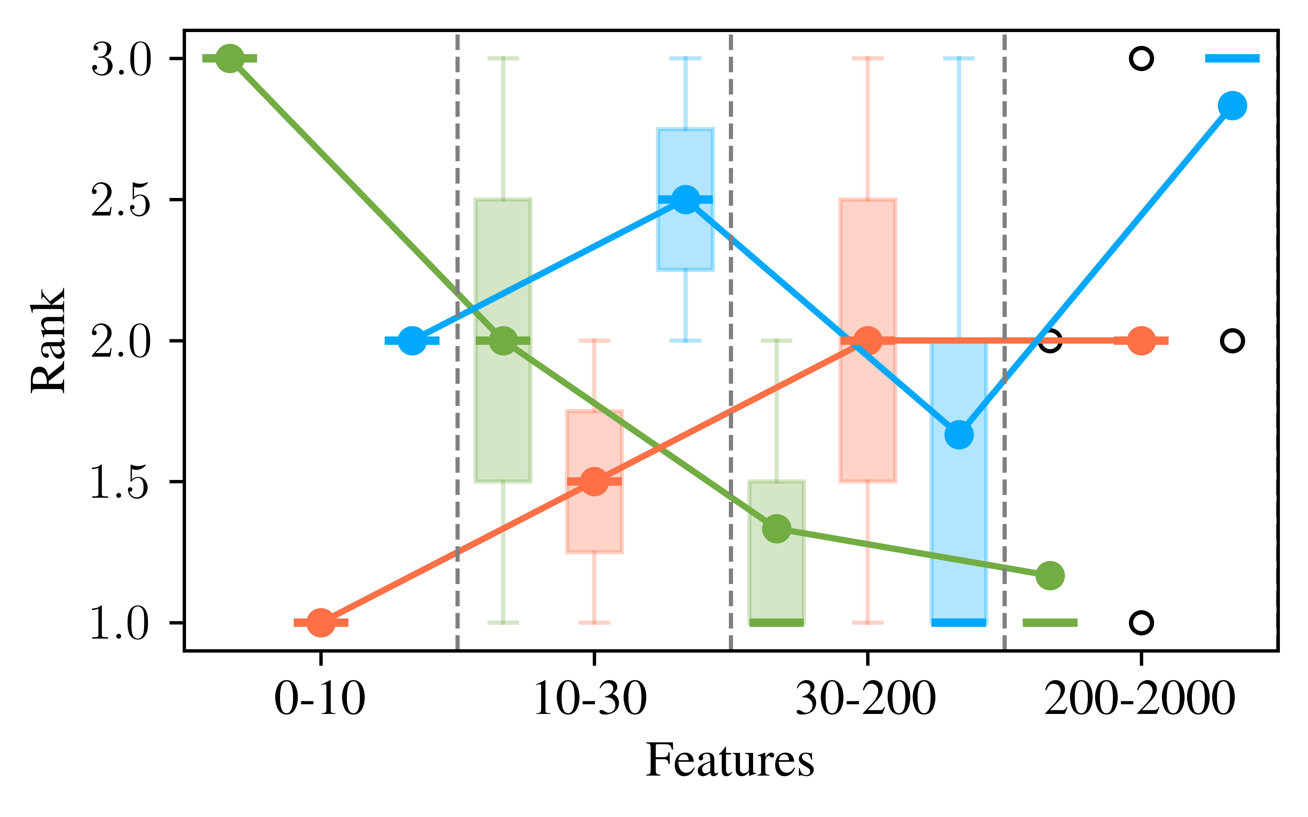
(a) LOF

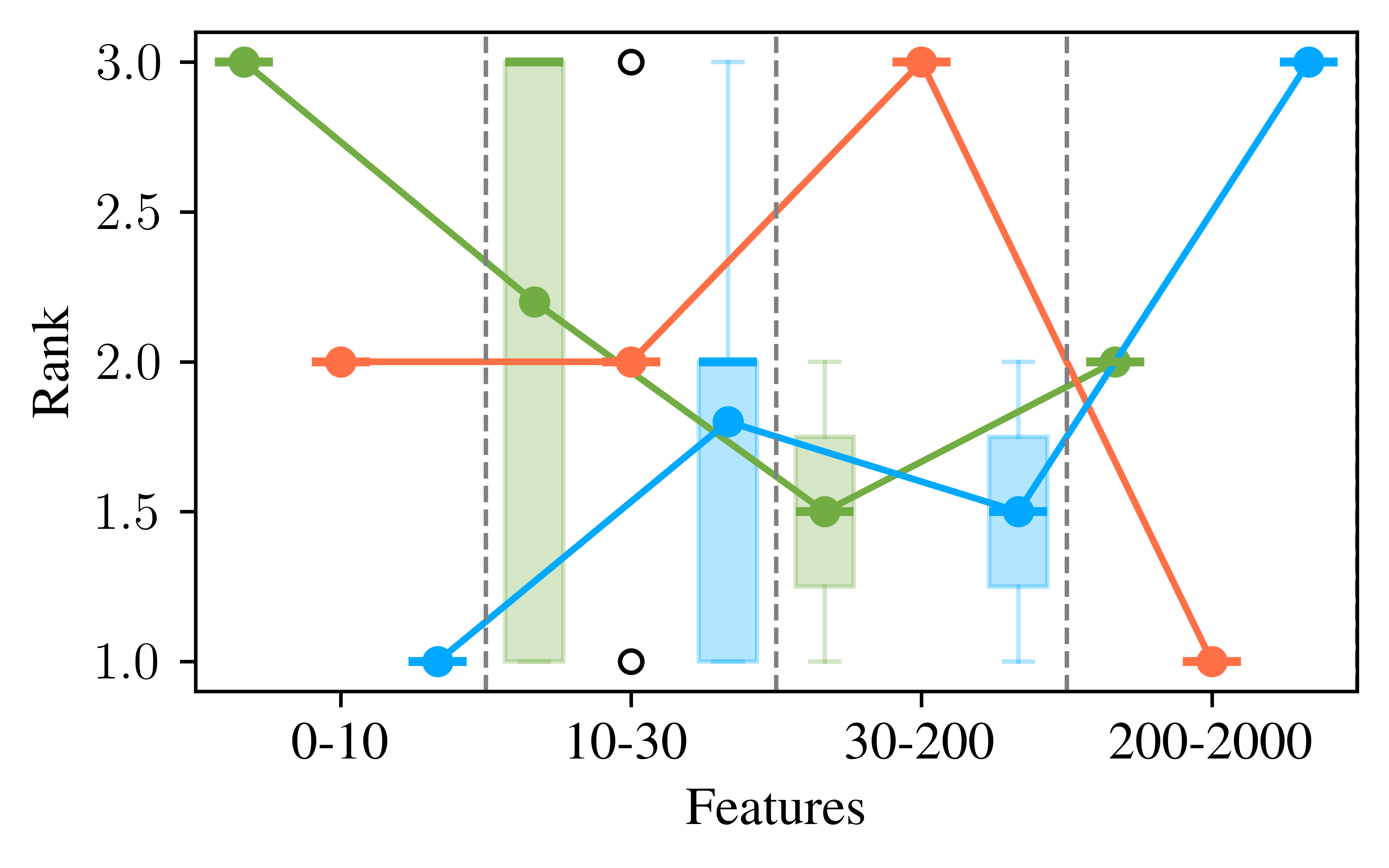
(b) kNN

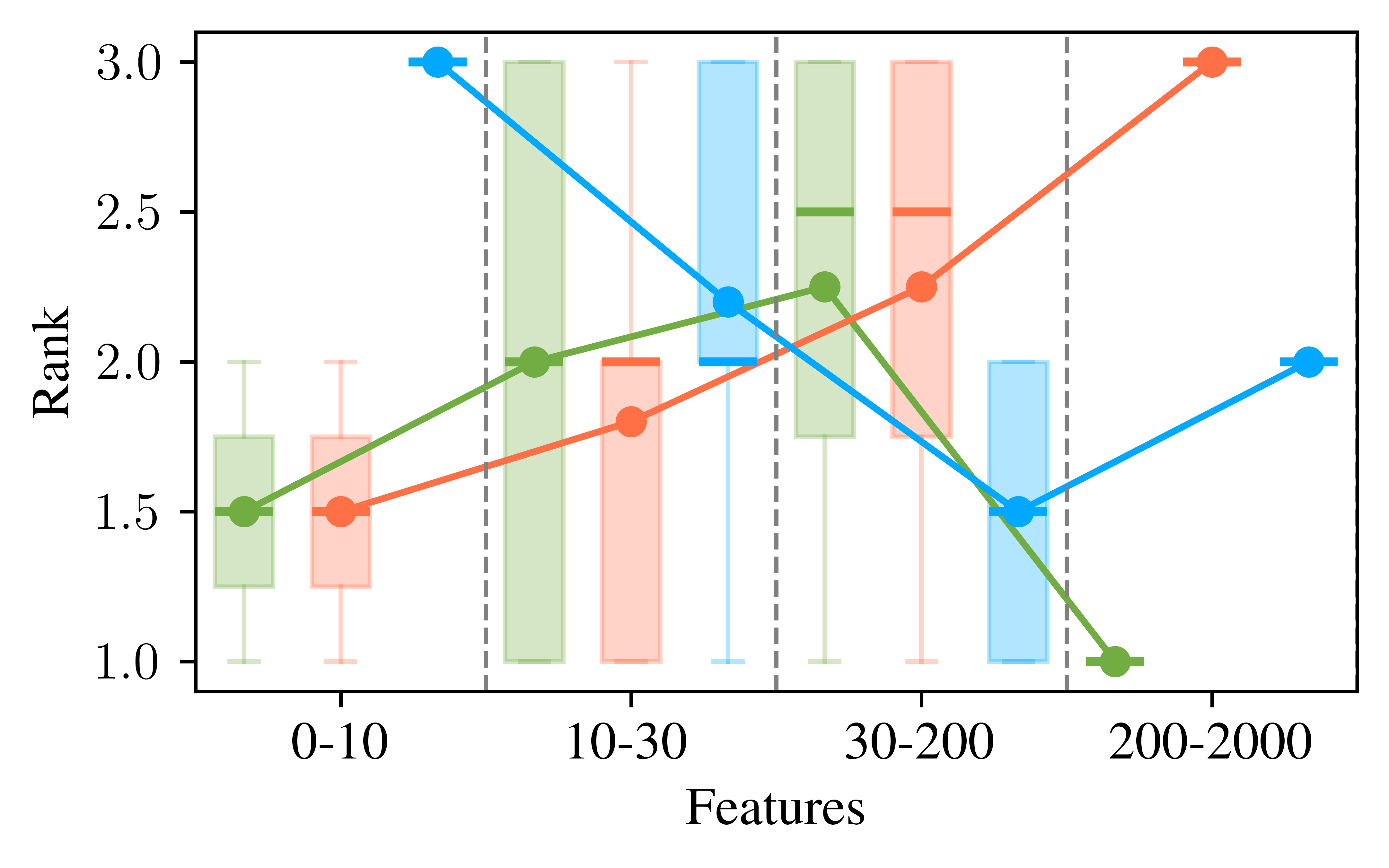
(c) ECOD

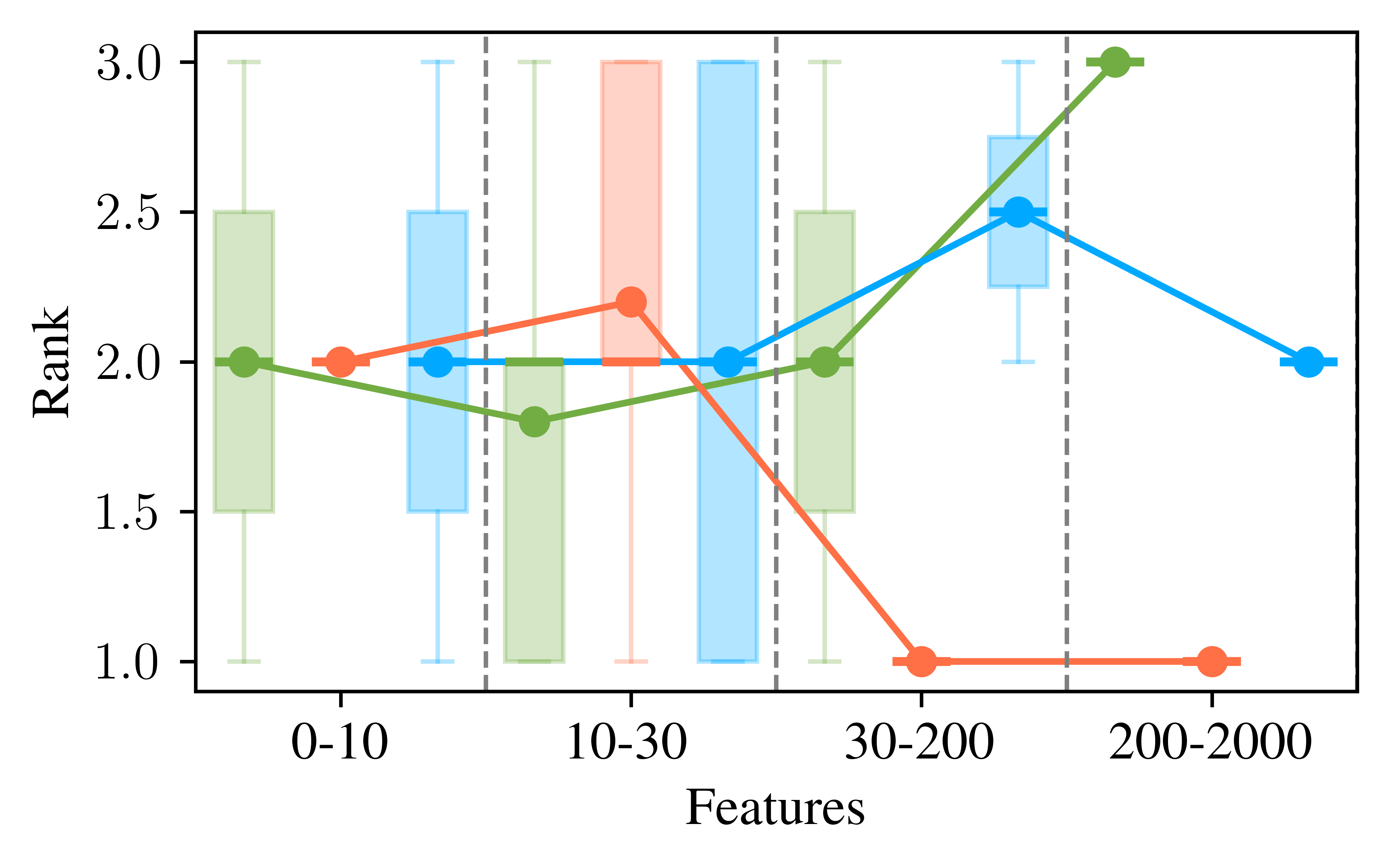
(d) COPOD

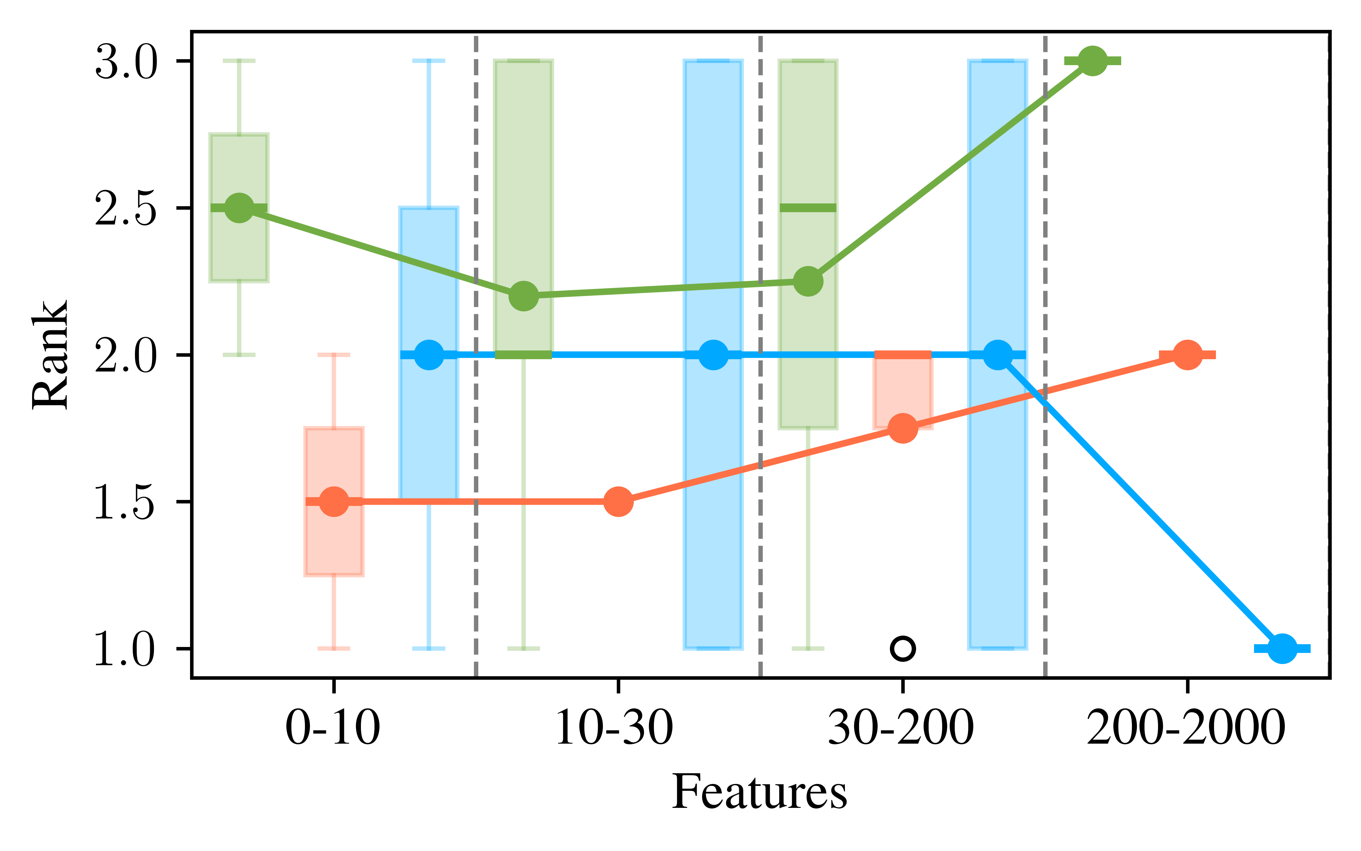
(e) CBLOF

(f) Legend

Figure 7: Boxplots of ranks of the comparison with baselines using non-myopic datasets across features

Table 5: Results of the Conover-Iman test for the rankings on non-myopic datasets

	LOF			kNN			ECOD			COPOD			CBLOF
	FB	None	V-GAN	FB	None	V-GAN	FB	None	V-GAN	FB	None	V-GAN	FB	None	V-GAN
FB		+ +												+
None	- -		- -										-		- -
V-GAN		+ +												++

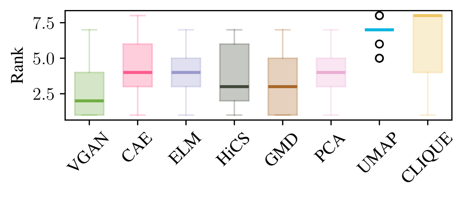
(a) LOF

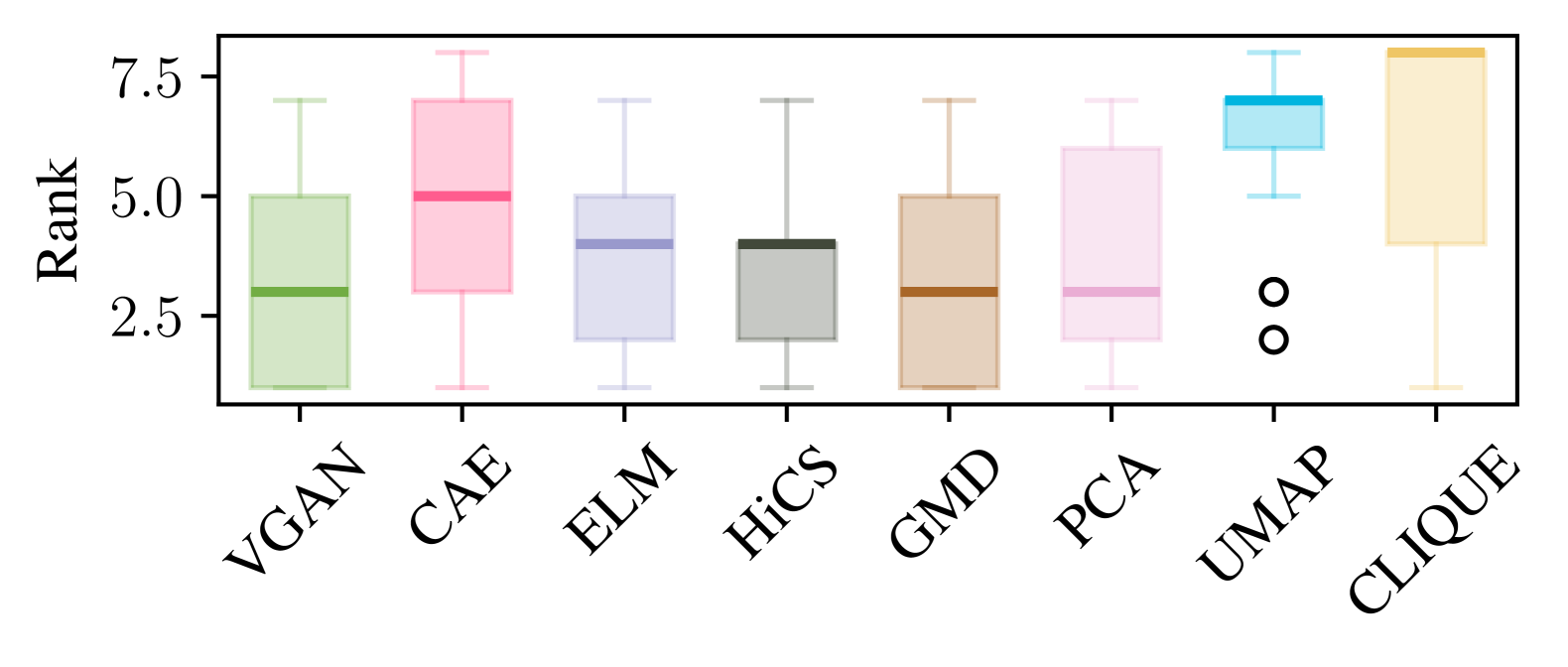
(b) kNN

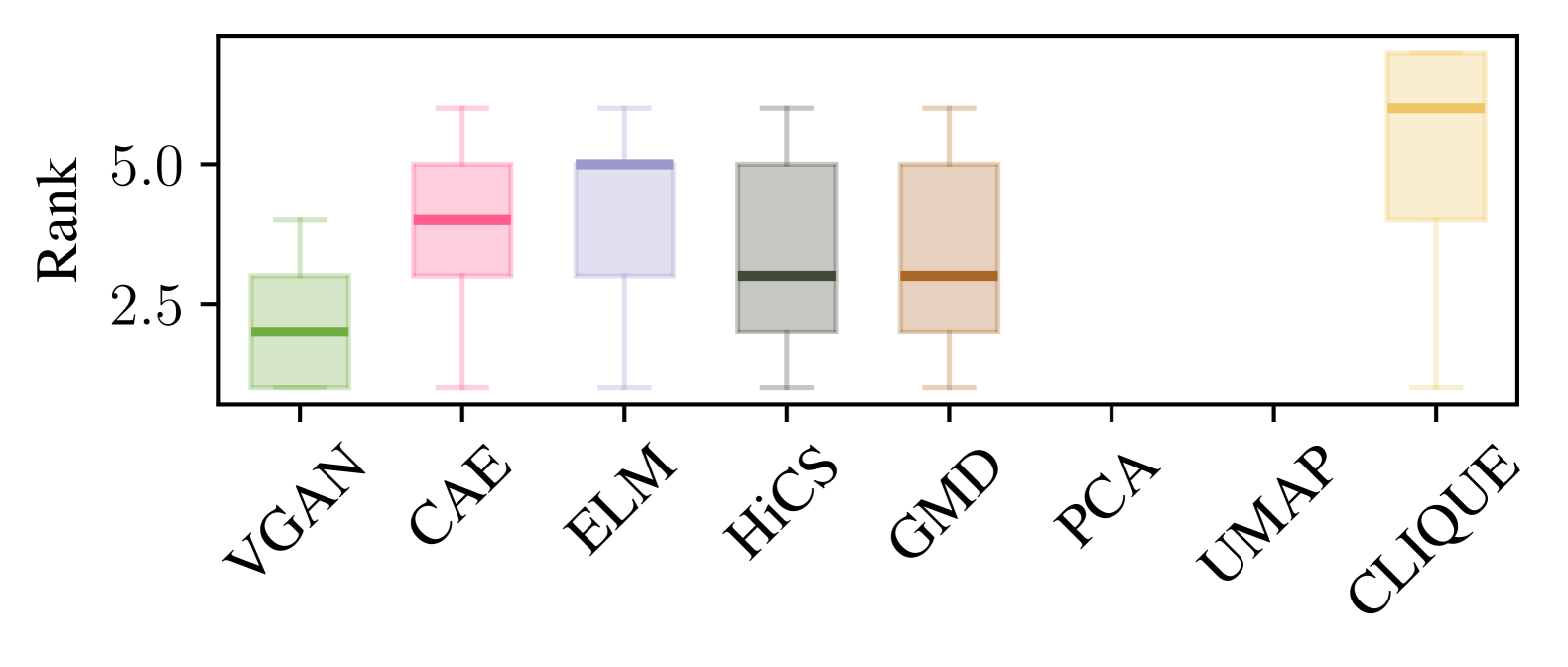
(c) ECOD

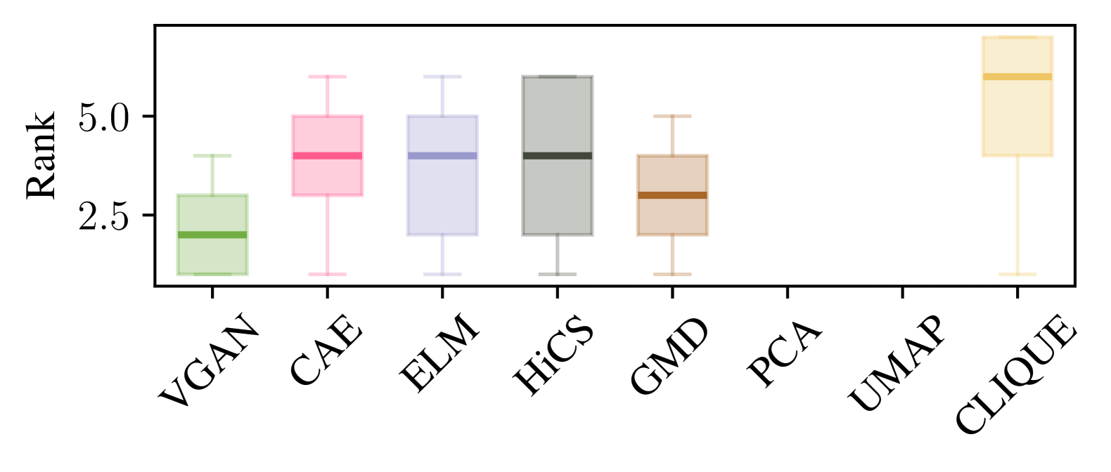
(d) COPOD

(e) CBLOF

Figure 8: Boxplots of ranks of the comparison with our competitors using non-myopic datasets.

Table 6: Results of the Conover-Iman Test for Rankings on non-Myopic Datasets

OD method	SS method	CAE	HiCS	CLIQUE	ELM	GMD	PCA	UMAP	V-GAN
LOF	CAE			++		-		++	- -
	HiCS			++				++
	CLIQUE	- -	- -		- -	- -	- -		- -
	ELM			++				++	-
	GMD	+		++				++
	PCA			++				++	-
	UMAP	- -	- -		- -	- -	- -		- -
	V-GAN	++		++	+		+	++
kNN	CAE		- -	++	-	- -	- -	+	- -
	HiCS	++		++				++
	CLIQUE	- -	- -		- -	- -	- -		- -
	ELM	+		++				++	- -
	GMD	++		++				++
	PCA	++		++				++
	UMAP	-	- -		- -	- -	- -		- -
	V-GAN	++		++				++
ECOD	CAE			++		-			- -
	HiCS			++					- -
	CLIQUE	- -	- -			- -			- -
	ELM					- -			- -
	GMD	+		++	++
	PCA
	UMAP
	V-GAN	++	++	++	++	++
COPOD	CAE			++		-			- -
	HiCS			++		-			- -
	CLIQUE	- -	- -		- -	- -			- -
	ELM			++					- -
	GMD	+	+	++
	PCA
	UMAP
	V-GAN	++	++	++	++
CBLOF	CAE					- -	- -		-
	HiCS			++	++			++
	CLIQUE		- -			- -	- -		- -
	ELM		- -			- -	- -		- -
	GMD	++		++	++			++
	PCA	++		++	++			++
	UMAP		- -			- -	- -		- -
	V-GAN	+		++	++			++

Table 7: Full table of raw AUCs from Section 5.3 using LOF. We denoted time-outs by OT, and ODM errors by ERR.

Dataset	Features	Feature Bagging	Full Space	CAE	CLIQUE	HiCS	GMD	PCA	UMAP	ELM	$\mathbf{V}$-GAN	Myopicity
InternetAds	1555	0.8613	0.7757	0.5154	OT	0.8300	0.8127	0.4632	0.4546	0.7642	0.8211	0
20news	768	0.7867	0.7861	0.6613	OT	0.5463	0.6609	0.6382	0.5219	0.7647	0.7902	1
Agnews	768	0.6920	0.6900	0.6336	OT	0.4863	0.5239	0.5489	0.5280	0.6841	0.6971	0
Amazon	768	0.5975	0.5975	0.5880	OT	0.5071	0.6302	0.5952	0.5226	0.5777	0.5998	0
Imdb	768	0.5433	0.5433	0.5555	OT	0.5086	0.5905	0.5720	0.5058	0.5345	0.5443	0
Yelp	768	0.6792	0.6782	0.6151	OT	0.5198	0.6704	0.6443	0.5196	0.6584	0.6825	0
CIFAR10	512	0.7389	0.7328	0.6122	OT	0.6624	0.6492	0.7449	0.5942	0.7415	0.7491	1
FashionMNIST	512	0.8891	0.8869	0.8636	OT	0.7863	0.9227	0.9048	0.8570	0.8923	0.8978	1
MNIST-C	512	0.9757	0.9752	0.8736	OT	0.6405	0.6187	0.7066	0.5099	0.9288	0.9762	1
MVTec-AD	512	0.9704	0.9700	0.9624	OT	0.9275	0.7539	0.8635	0.5969	0.9543	0.9713	0
SVHN	512	0.7168	0.7151	0.6474	OT	0.5891	0.5795	0.6981	0.5184	0.6766	0.7175	1
speech	400	0.5513	0.5243	0.5995	OT	0.5390	0.5812	0.3882	0.5325	0.5704	0.5895	1
musk	166	1.0000	1.0000	0.9988	OT	1.0000	1.0000	1.0000	0.6175	1.0000	1.0000	0
mnist	100	0.9681	0.9664	0.8394	OT	0.6373	0.7369	0.9126	0.5523	0.9638	0.9733	1
optdigits	64	0.9984	0.9988	0.9964	OT	0.5057	0.6032	0.9996	0.6970	0.9802	0.9986	0
SpamBase	57	0.4305	0.3608	0.3619	OT	0.8251	0.7897	0.3315	0.4732	0.5017	0.4901	0
landsat	36	0.7785	0.7744	0.7810	OT	0.8208	0.7447	0.7880	0.5257	0.6925	0.7792	1
satellite	36	0.8664	0.8686	0.8591	OT	0.8075	0.8148	0.8489	0.6293	0.5741	0.8702	1
satimage-2	36	0.9972	0.9968	0.9926	OT	0.9972	0.9977	0.9970	0.5501	0.9969	0.9974	1
Ionosphere	33	0.9311	0.9287	0.9190	OT	0.9376	0.5723	0.5227	0.4699	0.8865	0.9327	0
WPBC	33	0.5304	0.5326	0.4433	OT	0.5950	0.9384	0.8379	0.5290	0.5011	0.5370	0
letter	32	0.9221	0.9093	0.8523	OT	0.7813	0.7609	0.8387	0.6419	0.9207	0.9286	1
WDBC	30	0.9958	0.9944	0.9845	OT	1.0000	0.9915	0.9944	0.8313	0.9799	0.9956	0
fault	27	0.6647	0.6516	0.6378	OT	0.6107	0.6011	0.6312	0.5320	0.6316	0.6578	1
annthyroid	21	0.9357	0.8752	0.6605	0.9593	0.9629	0.7895	0.8107	0.5842	0.7229	0.9273	1
cardio	21	0.6727	0.6135	0.7542	OT	0.8836	0.8517	0.6721	0.5587	0.6425	0.6827	1
Cardiotocography	21	0.8004	0.7818	0.7275	OT	0.7638	0.8136	0.3545	0.6144	0.7033	0.8107	1
Waveform	21	0.8157	0.8131	0.6935	OT	0.8173	0.7599	0.7317	0.6614	0.8292	0.8173	1
Hepatitis	19	0.6432	0.6272	0.6923	OT	0.8107	0.8757	0.6331	0.4615	0.5083	0.6473	0
Lymphography	18	0.9756	0.9821	0.9018	OT	0.9524	0.9524	0.9464	0.7226	0.9643	0.9994	0
pendigits	16	0.9962	0.9916	0.8698	OT	0.9825	0.9698	0.9871	0.6882	0.9945	0.9699	1
wine	13	0.9737	0.9708	0.9792	0.9792	0.9625	0.9708	0.9708	0.7038	0.8008	0.9771	0
vowels	12	0.9653	0.9610	0.6538	0.9285	0.9196	0.9446	0.8443	0.6826	0.9639	0.9447	0
PageBlocks	10	0.9645	0.9411	0.9432	0.9789	0.9767	0.9708	0.9339	0.5048	0.7374	0.9662	1
breastw	9	0.8019	0.8059	0.7698	0.8391	0.8619	0.6721	0.7349	0.4886	0.7599	0.8726	0
Stamps	9	0.9802	0.9662	0.9136	0.9886	0.9579	0.9818	0.9287	0.5517	0.8256	0.9760	0
WBC	9	0.7370	0.7047	0.7372	0.7326	0.6884	0.8934	0.8453	0.5833	0.6912	0.5921	0
Pima	8	0.6422	0.6343	0.4597	0.6530	0.6365	0.6224	0.6253	0.5863	0.6225	0.6103	0
yeast	8	0.5097	0.4734	0.5299	0.5810	0.5464	0.5779	0.4715	0.5231	0.5186	0.5604	1
thyroid	6	0.9357	0.8752	0.6613	0.9593	0.9629	0.8493	0.6721	0.5587	0.7229	0.9173	1
vertebral	6	0.4958	0.4873	0.4915	0.4952	0.4944	0.4786	0.4841	0.4293	0.5696	0.4612	0
Wilt	5	0.8907	0.9054	0.7215	0.8728	0.8565	0.8398	0.5836	0.5540	0.7306	0.6122	1

Table 8: Full table of raw AUCs from Section 5.3 using kNN. We denoted time-outs by OT, and ODM errors by ERR.

Dataset	Features	Feature Bagging	Full Space	CAE	CLIQUE	HiCS	GMD	PCA	UMAP	ELM	$\mathbf{V}$-GAN	Myopicity
InternetAds	1555	0.8914	0.8801	0.6037	OT	0.8716	0.8814	0.5578	0.6910	0.8403	0.7420	0
20news	768	0.6852	0.6847	0.6659	OT	0.5213	0.6793	0.6120	0.4779	0.6819	0.6860	1
Agnews	768	0.5689	0.5696	0.5092	OT	0.4663	0.5304	0.5310	0.5286	0.5569	0.5650	0
Amazon	768	0.6019	0.6019	0.5717	OT	0.5328	0.5533	0.5303	0.5735	0.5860	0.6024	0
Imdb	768	0.5288	0.5285	0.5526	OT	0.5177	0.5898	0.5818	0.4757	0.5309	0.5294	0
Yelp	768	0.6668	0.6668	0.6019	OT	0.5526	0.6466	0.6398	0.4890	0.6448	0.6676	0
CIFAR10	512	0.7898	0.7882	0.6933	OT	0.7037	0.7854	0.8621	0.5670	0.7671	0.7913	1
FashionMNIST	512	0.9169	0.9161	0.8400	OT	0.8477	0.9031	0.9717	0.3872	0.9035	0.9171	1
MNIST-C	512	0.8960	0.8958	0.7859	OT	0.6464	0.7432	0.7812	0.5003	0.8568	0.8993	1
MVTec-AD	512	0.9748	0.9745	0.9658	OT	0.9279	0.8649	0.9083	0.5747	0.9666	0.9745	0
SVHN	512	0.7219	0.7205	0.6407	OT	0.6034	0.5880	0.7149	0.5700	0.6984	0.7220	1
speech	400	0.6570	0.6503	0.5486	OT	0.5346	0.6664	0.5636	0.6075	0.5857	0.6745	1
musk	166	1.0000	1.0000	1.0000	OT	1.0000	1.0000	1.0000	0.6791	1.0000	1.0000	0
mnist	100	0.9771	0.9779	0.8867	OT	0.8349	0.8685	0.9489	0.4804	0.9618	0.9780	1
optdigits	64	0.9979	0.9981	0.9975	OT	0.5289	0.9077	0.9994	0.7617	0.9844	0.9973	0
SpamBase	57	0.3579	0.3584	0.3758	OT	0.7329	0.4295	0.3511	0.4495	0.3057	0.3601	0
landsat	36	0.7850	0.7842	0.7815	OT	0.7824	0.7624	0.8215	0.5057	0.7715	0.7857	1
satellite	36	0.8290	0.8295	0.8304	OT	0.7941	0.8153	0.8243	0.5704	0.7882	0.8291	1
satimage-2	36	0.9993	0.9993	0.9992	OT	0.9983	0.9981	0.9990	0.1325	0.9993	0.9993	1
Ionosphere	33	0.9767	0.9771	0.9690	OT	0.9646	0.5702	0.5298	0.4509	0.9786	0.9777	0
WPBC	33	0.5091	0.5191	0.4801	OT	0.5709	0.9621	0.8760	0.6175	0.4955	0.5128	0
letter	32	0.9350	0.9305	0.9261	OT	0.8602	0.8608	0.8989	0.6701	0.9344	0.9364	1
WDBC	30	0.9742	0.9718	0.9338	OT	0.9958	0.9930	0.9803	0.4587	0.9168	0.9756	0
fault	27	0.8105	0.8093	0.7886	OT	0.7169	0.7058	0.7854	0.6394	0.8034	0.8098	1
annthyroid	21	0.7092	0.7681	0.5823	0.7954	0.8065	0.8263	0.8064	0.4749	0.6669	0.7167	1
cardio	21	0.8153	0.6976	0.5419	OT	0.8378	0.6687	0.6091	0.4294	0.6734	0.8166	1
Cardiotocography	21	0.7816	0.7187	0.7598	OT	0.7502	0.7903	0.4990	0.5295	0.6553	0.8087	1
Waveform	21	0.7190	0.8040	0.7220	OT	0.8592	0.7457	0.6822	0.4876	0.6996	0.7264	1
Hepatitis	19	0.7284	0.7337	0.6331	OT	0.7811	0.7929	0.5799	0.5959	0.6314	0.6580	0
Lymphography	18	0.9577	0.9583	0.7321	OT	0.9583	0.9524	0.9583	0.7399	0.9548	0.9804	0
pendigits	16	0.9987	0.9988	0.9805	OT	0.9943	0.9903	0.9991	0.6486	0.9969	0.9905	1
wine	13	0.9396	0.9417	0.9542	0.9417	0.9417	0.9708	0.9625	0.2663	0.4542	0.9337	0
vowels	12	0.9836	0.9806	0.7430	0.9572	0.9679	0.9717	0.9163	0.5841	0.9803	0.9572	0
PageBlocks	10	0.9720	0.9805	0.9646	0.9738	0.9547	0.9729	0.9665	0.2513	0.9549	0.9592	1
breastw	9	0.9876	0.9245	0.8457	0.9571	0.9644	0.9140	0.7860	0.6814	0.9066	0.9830	0
Stamps	9	0.8270	0.9880	0.9240	0.9886	0.9631	0.9657	0.9693	0.6981	0.9627	0.8640	0
WBC	9	0.9415	0.7814	0.6814	0.8767	0.9186	0.9735	0.9245	0.7544	0.7995	0.9686	0
Pima	8	0.5518	0.5593	0.4660	0.5431	0.5249	0.4781	0.5340	0.4849	0.5213	0.5151	0
yeast	8	0.5834	0.5871	0.5192	0.5710	0.5606	0.5787	0.5883	0.5355	0.5955	0.5833	1
thyroid	6	0.7816	0.7681	0.5823	0.7954	0.8065	0.7883	0.6091	0.4294	0.6669	0.8087	1
vertebral	6	0.5260	0.5333	0.4770	0.5278	0.5254	0.4913	0.5611	0.4828	0.5293	0.5214	0
Wilt	5	0.8434	0.8620	0.6910	0.8257	0.8493	0.7971	0.6548	0.5643	0.8578	0.7216	1

Table 9: Full table of raw AUCs from Section 5.3 using ECOD. We denoted time-outs by OT, and ODM errors by ERR.

Dataset	Features	Feature Bagging	Full Space	CAE	CLIQUE	HiCS	GMD	PCA	UMAP	ELM	$\mathbf{V}$-GAN	Myopicity
InternetAds	1555	0.6994	0.6990	0.3337	OT	0.7746	0.7114	ERR	0.2977	0.3670	0.6350	0
20news	768	0.6547	0.6547	0.6032	OT	0.4776	0.6198	0.6552	0.5953	0.6510	0.6556	1
Agnews	768	0.5089	0.5090	0.4934	OT	0.4646	0.5093	ERR	0.5182	0.4916	0.5094	0
Amazon	768	0.5635	0.5635	0.5604	OT	0.5015	0.4939	ERR	0.5065	0.5675	0.5640	0
Imdb	768	0.5052	0.5052	0.4834	OT	0.5130	0.5509	ERR	0.5334	0.4941	0.5043	0
Yelp	768	0.6023	0.6024	0.5605	OT	0.5023	0.5849	ERR	0.5488	0.5930	0.6020	0
CIFAR10	512	0.7228	0.7222	0.6382	OT	0.7027	0.6562	ERR	0.4936	0.7218	0.7229	1
FashionMNIST	512	0.8215	0.8213	0.6934	OT	0.8216	0.9393	ERR	0.5920	0.8118	0.8216	1
MNIST-C	512	0.6473	0.6470	0.5242	OT	0.6288	0.7073	ERR	0.4760	0.6364	0.6490	1
MVTec-AD	512	0.9399	0.9403	0.9331	OT	0.9234	0.8127	ERR	0.5296	0.8566	0.9415	0
SVHN	512	0.5609	0.5608	0.4566	OT	0.6007	0.5634	ERR	0.3949	0.5232	0.5653	1
speech	400	0.5451	0.5421	0.4884	OT	0.5325	0.5814	ERR	0.4251	0.5420	0.5420	1
musk	166	0.8685	0.8681	0.1663	OT	0.0430	0.6342	ERR	0.4911	0.1949	0.8683	0
mnist	100	0.7476	0.7478	0.7719	OT	0.6536	0.7024	ERR	0.5676	0.8846	0.7822	1
optdigits	64	0.5611	0.5608	0.4640	OT	0.4910	0.6191	ERR	ERR	0.3226	0.5615	0
SpamBase	57	0.5957	0.5962	0.2578	OT	0.8083	0.6351	ERR	ERR	0.3359	0.5943	0
landsat	36	0.4304	0.4310	0.4292	OT	0.5084	0.4487	ERR	ERR	0.3224	0.4326	1
satellite	36	0.6979	0.6983	0.6802	OT	0.6199	0.6801	ERR	ERR	0.6694	0.6985	1
satimage-2	36	0.9932	0.9931	0.9949	OT	0.9859	0.9916	ERR	ERR	0.9917	0.9932	1
Ionosphere	33	0.8406	0.8409	0.8335	OT	0.7944	0.4972	ERR	ERR	0.8720	0.8405	0
WPBC	33	0.5090	0.5085	0.4638	OT	0.4801	0.8097	ERR	ERR	0.4228	0.5077	0
letter	32	0.5106	0.5112	0.4830	OT	0.4861	0.4862	ERR	ERR	0.4993	0.5107	1
WDBC	30	0.9486	0.9479	0.9324	OT	0.9648	0.9620	ERR	ERR	0.9565	0.9477	0
fault	27	0.4431	0.4430	0.4110	OT	0.4056	0.4269	ERR	ERR	0.3800	0.4442	1
annthyroid	21	0.7514	0.7513	0.6448	0.7527	0.7513	0.6585	ERR	ERR	0.5977	0.7521	1
cardio	21	0.5101	0.5107	0.4407	OT	0.7397	0.6742	ERR	ERR	0.1092	0.5129	1
Cardiotocography	21	0.7369	0.7375	0.7176	OT	0.7322	0.7808	ERR	ERR	0.6140	0.7386	1
Waveform	21	0.7132	0.7128	0.6209	OT	0.6922	0.7235	ERR	ERR	0.7609	0.7118	1
Hepatitis	19	0.6361	0.6391	0.6391	OT	0.6095	0.6272	ERR	ERR	0.4450	0.6402	0
Lymphography	18	0.9327	0.9286	0.7857	OT	0.9643	0.9464	ERR	ERR	0.9452	0.9304	0
pendigits	16	0.8690	0.8709	0.8053	OT	0.8996	0.8998	ERR	ERR	0.8313	0.8725	1
wine	13	0.8913	0.8917	0.9292	0.8917	0.8708	0.8417	ERR	ERR	0.7492	0.8900	0
vowels	12	0.4608	0.4596	0.4044	0.4752	0.2231	0.3682	ERR	ERR	0.4261	0.4929	0
PageBlocks	10	0.9475	0.9472	0.9342	0.9472	0.9482	0.9356	ERR	ERR	0.9633	0.9468	1
breastw	9	0.7857	0.7884	0.2853	0.7836	0.8384	0.8953	ERR	ERR	0.3482	0.7856	0
Stamps	9	0.9085	0.9095	0.8387	0.9095	0.8715	0.8933	ERR	ERR	0.6948	0.9113	0
WBC	9	0.7944	0.7977	0.6442	0.7930	0.8349	0.8742	ERR	ERR	0.4526	0.7935	0
Pima	8	0.5485	0.5474	0.5256	0.5494	0.5422	0.5159	ERR	ERR	0.4825	0.5481	0
yeast	8	0.6006	0.6016	0.4625	0.5989	0.5843	0.5595	ERR	ERR	0.3393	0.6014	1
thyroid	6	0.7514	0.7513	0.6333	0.7527	0.7543	0.6732	ERR	ERR	0.5977	0.7501	1
vertebral	6	0.5171	0.5159	0.5774	0.5278	0.5143	0.5167	ERR	ERR	0.2838	0.5194	0
Wilt	5	0.3977	0.3970	0.3821	0.3970	0.4068	0.4109	ERR	ERR	0.4220	0.3968	1

Table 10: Full table of raw AUCs from Section 5.3 using COPOD. We denoted time-outs by OT, and ODM errors by ERR.

Dataset	Features	Feature Bagging	Full Space	CAE	CLIQUE	HiCS	GMD	PCA	UMAP	ELM	$\mathbf{V}$-GAN	Myopicity
InternetAds	1555	0.7000	0.6994	0.4041	OT	0.7748	0.7117	ERR	0.2415	0.4269	0.6356	0
20news	768	0.6480	0.6482	0.6107	OT	0.4755	0.6185	0.6030	0.5922	0.6347	0.6492	1
Agnews	768	0.5235	0.5235	0.4441	OT	0.4661	0.4985	ERR	0.5110	0.4818	0.5242	0
Amazon	768	0.5715	0.5715	0.5608	OT	0.4758	0.4984	ERR	0.5220	0.5719	0.5731	0
Imdb	768	0.5119	0.5118	0.5178	OT	0.4716	0.5488	ERR	0.5374	0.5029	0.5121	0
Yelp	768	0.6186	0.6186	0.5638	OT	0.4704	0.5913	ERR	0.5219	0.5945	0.6190	0
CIFAR10	512	0.7126	0.7128	0.6685	OT	0.7027	0.6481	ERR	0.4877	0.7454	0.7131	1
FashionMNIST	512	0.7996	0.7999	0.6227	OT	0.8216	0.9703	ERR	0.5923	0.7817	0.8002	1
MNIST-C	512	0.6441	0.6436	0.4702	OT	0.6288	0.6387	ERR	0.4320	0.6409	0.6440	1
MVTec-AD	512	0.9722	0.9720	0.9638	OT	0.9234	0.7939	ERR	0.5365	0.9460	0.9717	0
SVHN	512	0.5357	0.5362	0.4512	OT	0.6008	0.5407	ERR	0.4338	0.5969	0.5410	1
speech	400	0.5885	0.5891	0.5854	OT	0.5562	0.6189	ERR	0.3711	0.5453	0.5950	1
musk	166	0.7623	0.7597	0.1850	OT	0.1501	0.5693	ERR	0.4921	0.3524	0.7637	0
mnist	100	0.7418	0.7422	0.7218	OT	0.6248	0.6977	ERR	0.5500	0.8736	0.7430	1
optdigits	64	0.6509	0.6511	0.6553	OT	0.4930	0.6764	ERR	ERR	0.3467	0.6522	0
SpamBase	57	0.6223	0.6233	0.2214	OT	0.8106	0.6552	ERR	ERR	0.3679	0.6213	0
landsat	36	0.6420	0.6416	0.6065	OT	0.6256	0.6257	ERR	ERR	0.3353	0.6429	1
satellite	36	0.7318	0.7318	0.7100	OT	0.6295	0.7087	ERR	ERR	0.7075	0.7321	1
satimage-2	36	0.9944	0.9944	0.9952	OT	0.9861	0.9923	ERR	ERR	0.9978	0.9944	1
Ionosphere	33	0.8499	0.8499	0.8148	OT	0.8127	0.4468	ERR	ERR	0.8718	0.8497	0
WPBC	33	0.4465	0.4454	0.3652	OT	0.4376	0.8360	ERR	ERR	0.4087	0.4465	0
letter	32	0.5559	0.5558	0.5152	OT	0.5524	0.5355	ERR	ERR	0.5205	0.5564	1
WDBC	30	0.7954	0.7944	0.7915	OT	0.8324	0.8211	ERR	ERR	0.9445	0.7939	0
fault	27	0.4025	0.4020	0.3901	OT	0.3885	0.3710	ERR	ERR	0.3900	0.4034	1
annthyroid	21	0.7539	0.7522	0.5694	0.7528	0.7534	0.7704	ERR	ERR	0.5686	0.7599	1
cardio	21	0.7797	0.7808	0.3937	OT	0.7832	0.6177	ERR	ERR	0.1989	0.7837	1
Cardiotocography	21	0.6114	0.6103	0.7371	OT	0.6082	0.8992	ERR	ERR	0.6057	0.6097	1
Waveform	21	0.8284	0.8280	0.7212	OT	0.8003	0.5962	ERR	ERR	0.8110	0.8330	1
Hepatitis	19	0.6568	0.6627	0.4852	OT	0.6627	0.6391	ERR	ERR	0.4716	0.6621	0
Lymphography	18	0.9417	0.9405	0.6964	OT	0.9464	0.9167	ERR	ERR	0.9536	0.9423	0
pendigits	16	0.8993	0.8988	0.8096	OT	0.9187	0.9079	ERR	ERR	0.8613	0.8999	1
wine	13	0.5942	0.6083	0.7333	0.6083	0.5458	0.5833	ERR	ERR	0.6925	0.6042	0
vowels	12	0.4099	0.4005	0.3800	0.4285	0.2643	0.3070	ERR	ERR	0.4760	0.4176	0
PageBlocks	10	0.9534	0.9537	0.9270	0.9537	0.9559	0.9410	ERR	ERR	0.9659	0.9534	1
breastw	9	0.8441	0.8452	0.1872	0.8397	0.8876	0.8977	ERR	ERR	0.4579	0.8445	0
Stamps	9	0.9580	0.9579	0.9386	0.9579	0.9209	0.9542	ERR	ERR	0.9019	0.9579	0
WBC	9	0.8058	0.8047	0.7558	0.8023	0.8651	0.9179	ERR	ERR	0.5363	0.8044	0
Pima	8	0.5686	0.5681	0.5171	0.5710	0.5415	0.5441	ERR	ERR	0.4992	0.5701	0
yeast	8	0.4574	0.4576	0.4297	0.4631	0.4503	0.4833	ERR	ERR	0.3536	0.4589	1
thyroid	6	0.7539	0.7522	0.5694	0.7528	0.7534	0.6180	ERR	ERR	0.5686	0.7499	1
vertebral	6	0.4110	0.4111	0.4198	0.4087	0.3746	0.3952	ERR	ERR	0.3143	0.4105	0
Wilt	5	0.5192	0.5196	0.4749	0.5196	0.5302	0.5282	ERR	ERR	0.5057	0.5191	1

Table 11: Full table of raw AUCs from Section 5.3 using CBLOF. We denoted time-outs by OT, and ODM errors by ERR.

Dataset	Features	Feature Bagging	Full Space	CAE	CLIQUE	HiCS	GMD	PCA	UMAP	ELM	$\mathbf{V}$-GAN	Myopicity
InternetAds	1555	0.7347	0.7211	0.4141	OT	ERR	ERR	0.1804	0.3566	ERR	ERR	0
20news	768	0.6779	0.6680	0.5954	OT	0.4792	0.6906	0.6154	0.5232	0.6650	0.6788	1
Agnews	768	ERR	0.7543	0.4909	OT	0.5193	0.5323	0.5357	0.5312	ERR	ERR	0
Amazon	768	0.8843	0.8805	0.5550	OT	0.4940	0.5449	0.5138	0.5161	ERR	0.8864	0
Imdb	768	0.7984	0.7945	0.5489	OT	0.5211	0.5865	0.5667	0.5151	ERR	0.8015	0
Yelp	768	0.9767	0.9790	0.5595	OT	0.5265	0.6398	0.6092	0.5349	ERR	0.9757	0
CIFAR10	512	0.6997	0.6966	0.6747	OT	0.7061	ERR	0.7314	0.5709	ERR	ERR	1
FashionMNIST	512	ERR	0.5382	0.7742	OT	ERR	ERR	0.9738	0.6374	ERR	ERR	1
MNIST-C	512	1.0000	1.0000	0.7079	OT	ERR	0.7391	0.7547	0.5110	ERR	1.0000	1
MVTec-AD	512	ERR	0.9491	0.9679	OT	ERR	0.8407	0.8571	0.5750	0.9588	ERR	0
SVHN	512	ERR	0.9230	ERR	OT	ERR	0.5935	0.6729	0.5181	ERR	ERR	1
speech	400	0.3935	0.4077	ERR	OT	ERR	ERR	0.3581	0.5406	ERR	0.3924	1
musk	166	0.7634	0.7414	0.9234	OT	0.9981	1.0000	0.9998	0.3957	ERR	0.7628	0
mnist	100	0.8194	0.8170	ERR	OT	ERR	0.9247	ERR	0.5780	ERR	0.8196	1
optdigits	64	0.9989	0.9991	ERR	OT	ERR	0.8250	0.8529	0.7542	ERR	0.9995	0
SpamBase	57	0.9501	0.9631	0.4160	OT	0.6151	0.3576	0.4038	0.5056	0.3331	0.9486	0
landsat	36	0.5294	0.5759	0.7566	OT	0.8156	0.7337	0.7972	0.6178	0.7317	0.5258	1
satellite	36	0.8236	0.8009	0.8244	OT	0.7985	0.8072	0.8030	0.6327	0.7855	0.8298	1
satimage-2	36	0.9835	0.9915	0.9988	OT	0.9979	0.9979	0.9987	0.7356	0.9990	0.9797	1
Ionosphere	33	0.7743	0.7512	0.9155	OT	0.9434	0.5442	0.5255	0.4682	0.9647	0.7760	0
WPBC	33	0.6590	0.6615	0.5691	OT	0.5423	0.9523	0.8279	0.5247	0.4844	0.6631	0
letter	32	0.6793	0.6288	0.7445	OT	0.8223	0.8040	0.7145	0.5806	ERR	0.6990	1
WDBC	30	0.7224	0.8073	0.9266	OT	0.9901	0.9693	0.9859	0.6718	0.9513	0.7761	0
fault	27	ERR	0.7940	0.7229	OT	0.6983	0.6748	0.7142	0.5132	ERR	0.7979	1
annthyroid	21	0.7414	0.7219	0.6131	0.6682	0.6661	0.7971	0.7800	0.4919	0.6109	0.5769	1
cardio	21	0.9689	0.9643	0.5914	OT	ERR	0.6037	0.6129	0.6238	ERR	0.9804	1
Cardiotocography	21	0.9773	0.9798	0.6766	OT	ERR	0.8350	ERR	0.5623	0.6647	0.9506	1
Waveform	21	0.9317	0.8542	0.7152	OT	ERR	0.7812	0.7142	0.5700	ERR	0.9246	1
Hepatitis	19	ERR	0.9374	0.5811	OT	0.5030	0.7675	0.5503	0.4885	0.6166	0.8797	0
Lymphography	18	0.9710	0.9694	0.7905	OT	0.9583	0.9542	0.9762	0.7280	0.9548	0.9724	0
pendigits	16	0.9139	0.9011	0.9733	OT	ERR	0.9664	0.9795	0.4131	ERR	0.9291	1
wine	13	0.9886	0.9802	0.9342	0.9042	0.8639	0.8996	0.8375	0.1929	0.5398	0.9750	0
vowels	12	0.7842	0.6349	0.5752	ERR	ERR	0.9353	0.9288	0.6589	ERR	0.7914	0
PageBlocks	10	0.5891	0.5583	0.9484	0.9715	0.9698	0.9712	0.9664	0.8058	0.9725	0.5604	1
breastw	9	0.5777	0.5675	0.7112	0.9245	0.9364	0.8826	0.7395	0.5253	0.8548	0.5701	0
Stamps	9	0.6590	0.6615	0.9285	0.9888	0.9649	0.9728	0.9558	0.4891	0.9462	0.6591	0
WBC	9	0.5151	0.5254	0.5772	0.8281	0.8756	0.9587	0.8979	0.7153	0.7213	0.4733	0
Pima	8	0.7218	0.7151	0.4886	0.5906	0.5766	0.5696	0.5702	0.5443	0.5388	0.7403	0
yeast	8	0.5942	0.6083	0.5064	0.5590	0.5670	0.5786	0.5502	0.5429		0.6042	1
thyroid	6	0.4465	0.4454	0.6131	0.6687	0.6731	0.5980	0.6129	0.6238	0.6109	0.4465	1
vertebral	6	0.4574	0.4576	0.4322	0.5042	0.4927	0.4702	0.5825	0.4916	0.4952	0.4589	0
Wilt	5	0.6186	0.6186	0.5734	0.7171	0.7651	0.6892	0.5999	0.5858	0.7365	0.6190	1

B.2 Other Data types

This section aims to exemplify the flexibility of the Myopic Subspace Theory (MST) to adapt to different data types. In particular, we will present preliminary experiments for both Images and Natural Language in what follows. Our goal will be to exploit the human-friendly nature of images and text to visualize what a lens operator looks like in these cases. We include more specific details regarding all implementations and the training for both data types in their respective repositories. To encourage further research on MST, we are releasing all original data, code, and even model weights for all experiments for both data types.

B.2.1 $\mathbf{V}$-GAN vision: Myopic Subspace Theory on Image Data

We will first explore the results of applying $\mathbf{V}$-GAN to image data. For this experiment, we defined $E=\mathbb{R}^{3\cdot h\cdot w}$ and $\Theta(\mathfrak{X})=Diag_{(h\cdot w)\times(h\cdot w)}(\{0,1\})$, with $h$ and $w$ being the height and width of an image. Therefore, we are considering $E$ to be the vectorized space of all 3 RGB channels of an image, and $\Theta(\mathfrak{X})$ to be the space of $(h\cdot w)\times(h\cdot w)$ binary diagonal matrices acting on random images as:

$$\begin{split}\Theta(\mathfrak{X})\ni U:~&\mathfrak{X}\longrightarrow\mathfrak{X}\\ &x\leadsto Ux=(Ux_{\text{R}}\mid Ux_{\text{G}}\mid Ux_{\text{B}}).\end{split}$$ (14)

In other words, we are applying the operators simultaneously in all color channels. To make $\mathbf{V}$-GAN generate such subspaces, the only required change is to alter the head of the network to output a binary vector of the required size. In particular, we changed the layers of $\mathbf{V}$-GAN in order to better handle image data. In particular, we employ 5 sequential layers, each consisting of a linear layer for the learning, a Gaussian noise layer and a Batch Normalization layer for regularization, and a Leaky ReLU as an activation. After this, we include a last Batch Discrimination layer and a final linear layer, before passing the output into an upper softmax. The kernel that we use is a Gaussian kernel composed with an ImageNet-pretrained Autoencoder, and we did not employ kernel learning during training. We included a summary in Figure 9. We will study $\mathbf{V}$-GAN’s lens operators for image data with both real and synthetic data.

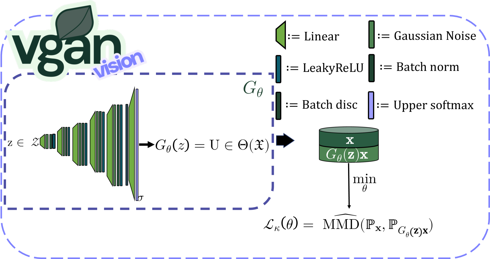
(a) Image data architecture

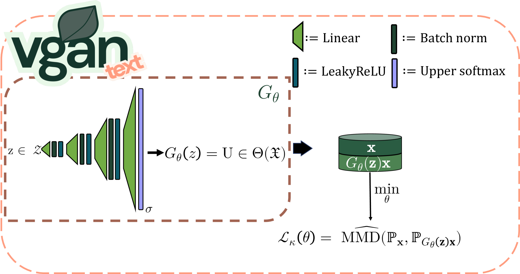
(b) Text data architecture

Figure 9: Diagram of the network for both image (left) and text (right) data.

Real Data.

We chose two popular datasets, FashionMNIST and MVTec-AD . The first consists of 28$\times$28 grey-scaled images of clothes, while the second consists of 900$\times$900 colored images of different industrial materials. We used the classes pants (images of pants) and bottle (cross-sections of steel bottles), respectively. Figure 10 contains the results for both FashionMNIST (Figure 10(a)) and MVTec-AD (Figure 10(b)). As we can see, the lens operators managed to extract interesting similarity patterns for each class. While in FashionMNIST, operators are mostly pant-shaped, in MVTec-AD, a more complex pattern emerged. Here, the operators selected different ring-shaped parts of the cross-sections rather than chunks of the image. These results further validate our theoretical claims that lens operators can extract complex relations in the data.

Synthetic Data.

To mirror the methodology in Section 5.2, we generated 10,000 synthetic images (32×32 pixels) with half-white/half-black sections. In particular, 5000 images had a white top part and a black bottom part, while the remaining 5000 had the inverse. Logically, as what happened with Section’s 5.2 population, one would expect that a lens operator consists of the two parts with equal probability. As we can see in Figure 11, the derived lens operator was exactly as we expected, further strengthening our derivations.

(a) FashionMNIST (28$\times$28)

(b) MVTec-AD (rescaled 64$\times$64)

Figure 10: Visualization of the lens operators obtained using $\mathbf{V}$-GAN in FashionMNIST and MVTec-AD. In the top row of both figures, we plotted 5 realizations of $\mathbf{U}$, and a final average between 500 samples. On the left-most column of both figures, we plotted 5 non-altered images. In the remaining columns and rows, we plotted each image after applying the corresponding operator in the column.

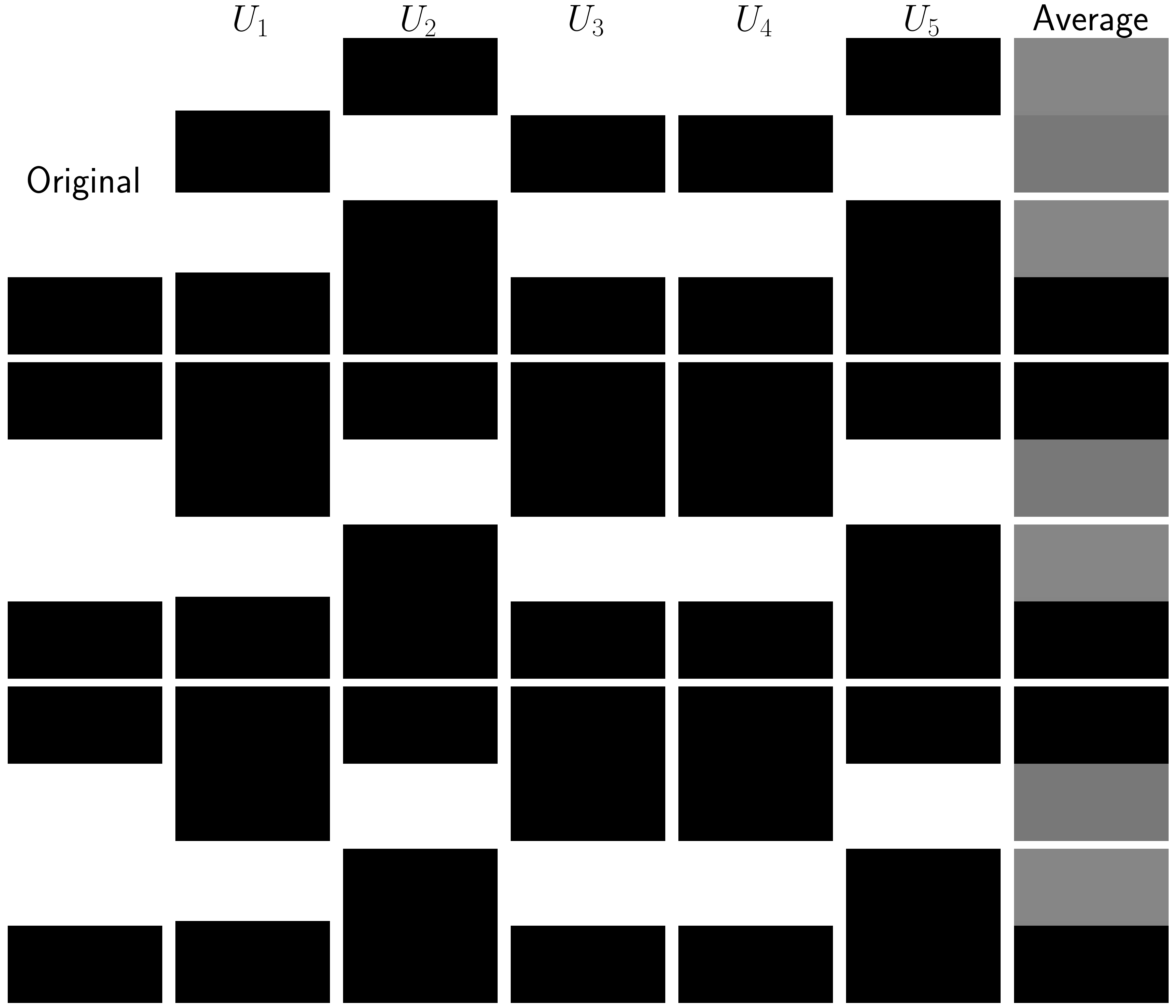
Figure 11: Visualization of the lens operators obtained using $\mathbf{V}$-GAN in synthetic data. In the top row of the figure, we plotted 5 realizations of $\mathbf{U}$, and a final average between 500 samples. On the left-most column, we plotted 5 non-altered images. In the remaining columns and rows, we plotted each image after applying the corresponding operator in the column.

B.2.2 $\mathbf{V}$-GAN text: Myopic Subspace Theory on Natural Language

We will try to extract lens operators from the token space of Natural Language data directly. We could do this by considering $E=\mathbb{N}^{s}$ and $\Theta(\mathfrak{X})=Diag_{s\times s}(\{0,1\})$, where $s$ is the predifined sentence length for each dataset. We also utilize a different architecture than before, featuring 3 sequential layers, each consisting in a Linear layer, a leaky ReLu and a Batch Normalization layer. After them, the outputs are passed into a final Linear layer with an upper softmax output for obtaining the operators. We use a simple gaussian kernel during training with no kernel learning.

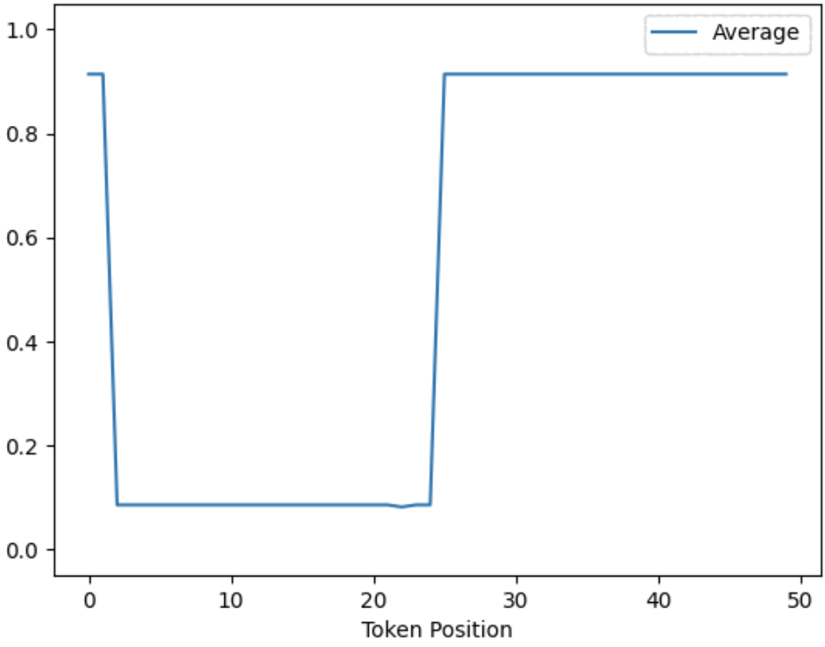
(a) Average selected token by $\mathbf{U}$ in AGnews

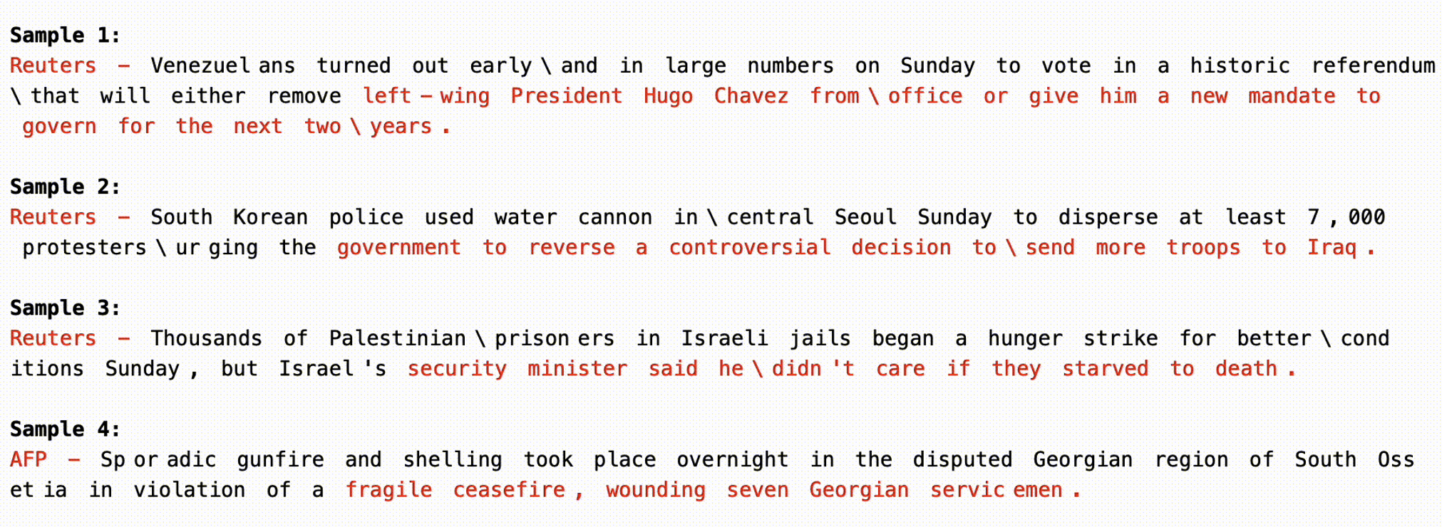
(b) Average selected token in AGnews’ text

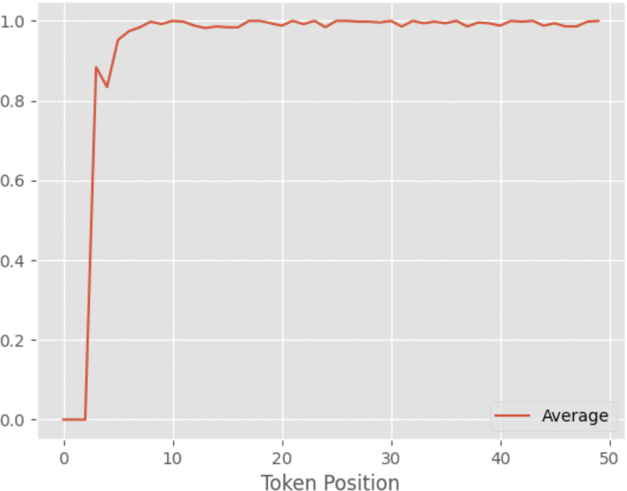
(c) Average selected token by $\mathbf{U}$ in Emotions

(d) Average selected token in Emotions’ text

Figure 12: Visualization of the lens operators obtained using $\mathbf{V}$-GAN in AGnews and Emotions. The first row corresponds to AGnews, and the second to Emotions. The left figures contain the average probability of selecting each token using $\mathbf{U}$. The right figures contain a visualization of the previous average probability on top of 4 text samples.

We planned similar experiments utilizing real data for Natural Language. In particular, we employed the AG news dataset and the Emotions dataset. The first one contains descriptions of news articles from different outlets, and the latter contains tweets about sentiments and feelings. Figure 12 contains the results for both.

In AGnews, Figure 12(a) shows how the derived lens operator $\mathbf{U}$ selects, on average, the beginning and the end of the sentence. By Figure 12(b), this means that $\mathbf{U}$ on average selects the news outlet — the beginning of each sample — and the core event of the news — the end of each sample. A similar behaviour can be observed for Emotions, where we can see that the network focuses on selecting the end of each tweet, corresponding to the actual feeling — see Figures 12(c) and 12(d). These results motivate the possible use of Myopic Subspace Theory also for Natural Language, further strengthening the applicability of this theory.

References

- Aggarwal [2017] C. C. Aggarwal. Outlier Analysis. Springer International Publishing, Cham, 2017. ISBN 978-3-319-47577-6 978-3-319-47578-3. doi: 10.1007/978-3-319-47578-3. URL http://link.springer.com/10.1007/978-3-319-47578-3.
- Agrawal et al. [2005] R. Agrawal, J. Gehrke, D. Gunopulos, and P. Raghavan. Automatic Subspace Clustering of High Dimensional Data. Data Mining and Knowledge Discovery, 11(1):5–33, July 2005. ISSN 1573-756X. doi: 10.1007/s10618-005-1396-1. URL https://doi.org/10.1007/s10618-005-1396-1.
- Arbel et al. [2019] M. Arbel, A. Korba, A. Salim, and A. Gretton. Maximum Mean Discrepancy Gradient Flow, Dec. 2019. URL http://arxiv.org/abs/1906.04370. arXiv:1906.04370 [cs, stat].
- Balın et al. [2019] M. F. Balın, A. Abid, and J. Zou. Concrete Autoencoders: Differentiable Feature Selection and Reconstruction. In Proceedings of the 36th International Conference on Machine Learning, pages 444–453. PMLR, May 2019. URL https://proceedings.mlr.press/v97/balin19a.html. ISSN: 2640-3498.
- Berlinet and Thomas-Agnan [2004] A. Berlinet and C. Thomas-Agnan. Reproducing Kernel Hilbert Spaces in Probability and Statistics. Springer US, Boston, MA, 2004. ISBN 978-1-4613-4792-7 978-1-4419-9096-9. doi: 10.1007/978-1-4419-9096-9. URL http://link.springer.com/10.1007/978-1-4419-9096-9.
- Bińkowski et al. [2021] M. Bińkowski, D. J. Sutherland, M. Arbel, and A. Gretton. Demystifying MMD GANs, Jan. 2021. URL http://arxiv.org/abs/1801.01401. arXiv:1801.01401 [cs, stat].
- Breunig et al. [2000] M. M. Breunig, H.-P. Kriegel, R. T. Ng, and J. Sander. LOF: identifying density-based local outliers. SIGMOD Rec., 29(2):93–104, May 2000. ISSN 0163-5808. doi: 10.1145/335191.335388. URL https://dl.acm.org/doi/10.1145/335191.335388.
- Campos et al. [2016] G. O. Campos, A. Zimek, J. Sander, R. J. G. B. Campello, B. Micenková, E. Schubert, I. Assent, and M. E. Houle. On the evaluation of unsupervised outlier detection: measures, datasets, and an empirical study. Data Mining and Knowledge Discovery, 30(4):891–927, July 2016. ISSN 1573-756X. doi: 10.1007/s10618-015-0444-8. URL https://doi.org/10.1007/s10618-015-0444-8.
- Chen et al. [2020] T. Chen, S. Kornblith, M. Norouzi, and G. Hinton. A Simple Framework for Contrastive Learning of Visual Representations. In Proceedings of the 37th International Conference on Machine Learning, pages 1597–1607. PMLR, Nov. 2020. URL https://proceedings.mlr.press/v119/chen20j.html. ISSN: 2640-3498.
- Conover and Iman [1979] W. J. Conover and R. L. Iman. Multiple-comparisons procedures. Technical Report LA-7677-MS, Los Alamos National Lab. (LANL), Los Alamos, NM (United States), Feb. 1979. URL https://www.osti.gov/biblio/6057803.
- Cribeiro-Ramallo et al. [2024] J. Cribeiro-Ramallo, V. Arzamasov, F. Matteucci, D. Wambold, and K. Böhm. Generative subspace adversarial active learning for outlier detection in multiple views of high-dimensional data, 2024. URL https://arxiv.org/abs/2404.14451.
- Elhamifar and Vidal [2013] E. Elhamifar and R. Vidal. Sparse Subspace Clustering: Algorithm, Theory, and Applications, Feb. 2013. URL http://arxiv.org/abs/1203.1005. arXiv:1203.1005 [cs, math, stat].
- Faden [1985] A. M. Faden. The Existence of Regular Conditional Probabilities: Necessary and Sufficient Conditions. The Annals of Probability, 13(1):288–298, Feb. 1985. ISSN 0091-1798, 2168-894X. doi: 10.1214/aop/1176993081. URL https://projecteuclid.org/journals/annals-of-probability/volume-13/issue-1/The-Existence-of-Regular-Conditional-Probabilities--Necessary-and-Sufficient/10.1214/aop/1176993081.full. Publisher: Institute of Mathematical Statistics.
- F.R.S. [1901] K. P. F.R.S. Liii. on lines and planes of closest fit to systems of points in space. The London, Edinburgh, and Dublin Philosophical Magazine and Journal of Science, 2(11):559–572, 1901. doi: 10.1080/14786440109462720.
- Fukumizu et al. [2007] K. Fukumizu, A. Gretton, X. Sun, and B. Schölkopf. Kernel Measures of Conditional Dependence. In Advances in Neural Information Processing Systems, volume 20. Curran Associates, Inc., 2007. URL https://papers.nips.cc/paper_files/paper/2007/hash/3a0772443a0739141292a5429b952fe6-Abstract.html.
- Garreau et al. [2018] D. Garreau, W. Jitkrittum, and M. Kanagawa. Large sample analysis of the median heuristic, Oct. 2018. URL http://arxiv.org/abs/1707.07269. arXiv:1707.07269 [math] version: 3.
- Goodfellow et al. [2016] I. Goodfellow, Y. Bengio, and A. Courville. Deep Learning. MIT Press, 2016. http://www.deeplearningbook.org.
- Gretton et al. [2012] A. Gretton, K. M. Borgwardt, M. J. Rasch, B. Schölkopf, and A. Smola. A Kernel Two-Sample Test. Journal of Machine Learning Research, 13(25):723–773, 2012. ISSN 1533-7928. URL http://jmlr.org/papers/v13/gretton12a.html.
- Guo et al. [2022] L. Guo, W. Song, and J. Shi. Estimating multivariate density and its derivatives for mixed measurement error data. Journal of Multivariate Analysis, 191:105005, Sept. 2022. ISSN 0047-259X. doi: 10.1016/j.jmva.2022.105005. URL https://www.sciencedirect.com/science/article/pii/S0047259X22000367.
- Han et al. [2022] S. Han, X. Hu, H. Huang, M. Jiang, and Y. Zhao. ADBench: Anomaly Detection Benchmark, Sept. 2022. URL http://arxiv.org/abs/2206.09426. arXiv:2206.09426 [cs].
- He et al. [2003] Z. He, X. Xu, and S. Deng. Discovering cluster-based local outliers. Pattern Recognition Letters, 24(9):1641–1650, June 2003. ISSN 0167-8655. doi: 10.1016/S0167-8655(03)00003-5. URL https://www.sciencedirect.com/science/article/pii/S0167865503000035.
- Healy and McInnes [2024] J. Healy and L. McInnes. Uniform manifold approximation and projection. Nature Reviews Methods Primers, 4(1):1–15, Nov. 2024. ISSN 2662-8449. doi: 10.1038/s43586-024-00363-x. URL https://www.nature.com/articles/s43586-024-00363-x. Publisher: Nature Publishing Group.
- Jones and Artemiou [2021] B. Jones and A. Artemiou. Revisiting the predictive power of kernel principal components. Statistics & Probability Letters, 171:109019, Apr. 2021. ISSN 0167-7152. doi: 10.1016/j.spl.2020.109019. URL https://www.sciencedirect.com/science/article/pii/S0167715220303229.
- Keller et al. [2012] F. Keller, E. Muller, and K. Bohm. HiCS: High Contrast Subspaces for Density-Based Outlier Ranking. In 2012 IEEE 28th International Conference on Data Engineering, pages 1037–1048, Apr. 2012. doi: 10.1109/ICDE.2012.88. URL https://ieeexplore.ieee.org/abstract/document/6228154. ISSN: 2375-026X.
- Kruskal and Wallis [1952] W. H. Kruskal and W. A. Wallis. Use of ranks in one-criterion variance analysis. Journal of the American Statistical Association, 47(260):583–621, 1952. doi: 10.1080/01621459.1952.10483441. URL https://www.tandfonline.com/doi/abs/10.1080/01621459.1952.10483441.
- Lazarevic and Kumar [2005] A. Lazarevic and V. Kumar. Feature bagging for outlier detection. In Proceedings of the eleventh ACM SIGKDD international conference on Knowledge discovery in data mining, KDD ’05, pages 157–166, New York, NY, USA, Aug. 2005. Association for Computing Machinery. ISBN 978-1-59593-135-1. doi: 10.1145/1081870.1081891. URL https://doi.org/10.1145/1081870.1081891.
- Li et al. [2017] C.-L. Li, W.-C. Chang, Y. Cheng, Y. Yang, and B. Póczos. MMD GAN: Towards Deeper Understanding of Moment Matching Network, Nov. 2017. URL http://arxiv.org/abs/1705.08584. arXiv:1705.08584 [cs, stat].
- Li et al. [2020] Z. Li, Y. Zhao, N. Botta, C. Ionescu, and X. Hu. COPOD: copula-based outlier detection. In IEEE International Conference on Data Mining (ICDM). IEEE, 2020.
- Li et al. [2023] Z. Li, Y. Zhao, X. Hu, N. Botta, C. Ionescu, and G. H. Chen. ECOD: Unsupervised Outlier Detection Using Empirical Cumulative Distribution Functions. IEEE Transactions on Knowledge and Data Engineering, 35(12):12181–12193, Dec. 2023. ISSN 1558-2191. doi: 10.1109/TKDE.2022.3159580. URL https://ieeexplore.ieee.org/document/9737003. Conference Name: IEEE Transactions on Knowledge and Data Engineering.
- Maćkiewicz and Ratajczak [1993] A. Maćkiewicz and W. Ratajczak. Principal components analysis (PCA). Computers & Geosciences, 19(3):303–342, Mar. 1993. ISSN 0098-3004. doi: 10.1016/0098-3004(93)90090-R. URL https://www.sciencedirect.com/science/article/pii/009830049390090R.
- Meilă and Zhang [2023] M. Meilă and H. Zhang. Manifold learning: what, how, and why, Nov. 2023. URL http://arxiv.org/abs/2311.03757. arXiv:2311.03757.
- Mroueh and Nguyen [2021] Y. Mroueh and T. Nguyen. On the Convergence of Gradient Descent in GANs: MMD GAN As a Gradient Flow. In Proceedings of The 24th International Conference on Artificial Intelligence and Statistics, pages 1720–1728. PMLR, Mar. 2021. URL https://proceedings.mlr.press/v130/mroueh21a.html. ISSN: 2640-3498.
- Müller et al. [2012] E. Müller, I. Assent, P. Iglesias, Y. Mülle, and K. Böhm. Outlier Ranking via Subspace Analysis in Multiple Views of the Data. In 2012 IEEE 12th International Conference on Data Mining, pages 529–538, Dec. 2012. doi: 10.1109/ICDM.2012.112. URL https://ieeexplore.ieee.org/document/6413873/?arnumber=6413873. ISSN: 2374-8486.
- Nguyen et al. [2014] H.-V. Nguyen, E. Müller, and K. Böhm. A Near-Linear Time Subspace Search Scheme for Unsupervised Selection of Correlated Features. Big Data Research, 1:37–51, Aug. 2014. ISSN 2214-5796. doi: 10.1016/j.bdr.2014.07.004. URL https://www.sciencedirect.com/science/article/pii/S2214579614000057.
- Pedregosa et al. [2011] F. Pedregosa, G. Varoquaux, A. Gramfort, V. Michel, B. Thirion, O. Grisel, M. Blondel, P. Prettenhofer, R. Weiss, V. Dubourg, J. Vanderplas, A. Passos, D. Cournapeau, M. Brucher, M. Perrot, and E. Duchesnay. Scikit-learn: Machine learning in Python. Journal of Machine Learning Research, 12:2825–2830, 2011.
- Perera et al. [2021] P. Perera, P. Oza, and V. M. Patel. One-Class Classification: A Survey, Jan. 2021. URL http://arxiv.org/abs/2101.03064. arXiv:2101.03064 [cs].
- Qu et al. [2023] W. Qu, X. Xiu, H. Chen, and L. Kong. A Survey on High-Dimensional Subspace Clustering. Mathematics, 11(2):436, Jan. 2023. ISSN 2227-7390. doi: 10.3390/math11020436. URL https://www.mdpi.com/2227-7390/11/2/436. Number: 2 Publisher: Multidisciplinary Digital Publishing Institute.
- Schrab et al. [2023] A. Schrab, I. Kim, M. Albert, B. Laurent, B. Guedj, and A. Gretton. MMD Aggregated Two-Sample Test, Aug. 2023. URL http://arxiv.org/abs/2110.15073. arXiv:2110.15073 [cs, math, stat].
- Simonnet [1996] M. Simonnet. Measures and Probabilities. Universitext. Springer, New York, NY, 1996. ISBN 978-0-387-94644-3 978-1-4612-4012-9. doi: 10.1007/978-1-4612-4012-9. URL http://link.springer.com/10.1007/978-1-4612-4012-9.
- Sriperumbudur et al. [2010] B. K. Sriperumbudur, A. Gretton, K. Fukumizu, B. Schölkopf, and G. R. Lanckriet. Hilbert Space Embeddings and Metrics on Probability Measures. J. Mach. Learn. Res., 11:1517–1561, Aug. 2010. ISSN 1532-4435.
- Trittenbach and Böhm [2019] H. Trittenbach and K. Böhm. Dimension-based subspace search for outlier detection. International Journal of Data Science and Analytics, 7(2):87–101, Mar. 2019. ISSN 2364-4168. doi: 10.1007/s41060-018-0137-7. URL https://doi.org/10.1007/s41060-018-0137-7.
- Xu et al. [2023] H. Xu, G. Pang, Y. Wang, and Y. Wang. Deep Isolation Forest for Anomaly Detection. IEEE Transactions on Knowledge and Data Engineering, 35(12):12591–12604, Dec. 2023. ISSN 1558-2191. doi: 10.1109/TKDE.2023.3270293. URL https://ieeexplore.ieee.org/document/10108034. Conference Name: IEEE Transactions on Knowledge and Data Engineering.
- Zeiler [2012] M. D. Zeiler. ADADELTA: An Adaptive Learning Rate Method, Dec. 2012. URL http://arxiv.org/abs/1212.5701. arXiv:1212.5701 [cs].