Stability and Convergence of Strang Splitting Method for the Allen–Cahn Equation with Homogeneous Neumann Boundary Condition

Abstract

The Strang splitting method has been widely used to solve nonlinear reaction-diffusion equations, with most theoretical convergence analysis assuming periodic boundary conditions. However, such analysis presents additional challenges for the case of homogeneous Neumann boundary condition. In this work the Strang splitting method with variable time steps is investigated for solving the Allen–Cahn equation with homogeneous Neumann boundary conditions. Uniform $H^{k}$-norm stability is established under the assumption that the initial condition $u^{0}$ belongs to the Sobolev space $H^{k}(\Omega)$ with integer $k\geq 0$, using the Gagliardo–Nirenberg interpolation inequality and the Sobolev embedding inequality. Furthermore, rigorous convergence analysis is provided in the $H^{k}$-norm for initial conditions $u^{0}\in H^{k+6}(\Omega)$, based on the uniform stability. Several numerical experiments are conducted to verify the theoretical results, demonstrating the effectiveness of the proposed method.

65M12, 65M15

1 Introduction

In this work, we consider the following Allen–Cahn equation [2] with homogeneous Neumann boundary condition

(1) $$\left\{\begin{aligned} &\partial_{t}u=\varepsilon^{2}\Delta u-f(u),&&(t,x)\in(0,T)\times\Omega,\\ &u(0,x)=u^{0}(x),&&\mbox{in }\Omega,\\ &\frac{\partial u}{\partial\mathbf{n}}=0,&&\mbox{on }\Gamma,\end{aligned}\right.$$

whose energy functional is

(2) $$E(u)=\int_{\Omega}\left(\frac{\varepsilon^{2}}{2}|\nabla u|^{2}+F(u)\right)\,{\mathrm{d}}x.$$

Here, the spatial domain $\Omega$ is a bounded open set in ${\mathbb{R}^{d}}~(d\leq 3)$ with a $C^{1}$ boundary, $\mathbf{n}$ is the unit outward normal vector on the boundary $\Gamma$, $f(u)=u^{3}-u$ is taken as the derivative of the potential $F(u)=\frac{1}{4}(u^{2}-1)^{2}$, and the parameter $\varepsilon^{2}$ is the mobility constant coefficient. It is well-known that the Allen–Cahn equation is the $L^{2}$ gradient flow of $E(u)$.

Operator splitting methods have been widely applied to solve differential equations. The key concept of operator splitting is to decompose a differential equation into a sequence of simpler problems [45, 12]. Two well-known splitting methods are the Lie–Trotter scheme [47] and Strang splitting [50]. For the Hamilton–Jacobi system, Glowinski, Leung and Qian develop an operator splitting method for computing effective Hamiltonians based on the Lie scheme in [25], which is applicable to both convex and non-convex Hamiltonians. For the Hamiltonian system describing the pendulum, one natural splitting form comes from separating the contributions of the kinetic energy and the potential energy. In this case, the Strang splitting scheme reduces to the Störmer–Verlet method [27]. For time-dependent Schrödinger equations, it has been proved that Strang splitting achieves second-order time accuracy when applied to pseudo-spectral discretizations of the Schrödinger equation [32, 4]. Moreover, higher-order splittings have been developed for the semiclassical time-dependent Schrödinger equation in [13]. Operator splitting methods are also effective within quantum physics, including Gross–Pitaevskii equation [7], the Dirac equation [5] and the Klein–Gordon equation [6]. For the reaction-diffusion equations, Liu, Wang and Wang in [43] propose and analyze a positivity-preserving, energy-stable numerical scheme for a certain type of reaction-diffusion system, followed by a detailed convergence analysis [44]. In [40], Li, Qiao and Zhang prove the global error estimate in discrete $L^{2}$-norm for the Strang splitting for the epitaxial growth model with slope selection on uniform time meshes. In [35], Lan et al. use operator splitting to solve the mass-conserving convective Allen–Cahn equation, which preserves the discrete maximum principle and conserves the mass.

In addition to operator splitting method [18, 40, 36, 37], we mention that a variety of structure-preserving numerical schemes have been well-developed for solving gradient flows, including the implicit-explicit (IMEX) methods [16, 51, 23], invariant energy quadratization (IEQ) method [53], scalar auxiliary variable (SAV) method [49, 1], integrating factor Runge–Kutta (IFRK) method [33, 39], exponential time differencing (ETD) method [19, 38, 24, 22] and so on.

Suppose time levels $0=t_{0}<t_{1}<t_{2}<\cdots<t_{N}=T$ with the time steps $\tau_{k}\coloneqq t_{k}-t_{k-1}$ for $1\leq k\leq N$. The Strang splitting is written as

(3) $$u^{n+1}=\mathcal{S}_{\mathcal{L}}\left(\frac{\tau_{n+1}}{2}\right)\mathcal{S}_{\mathcal{N}}\left(\tau_{n+1}\right)\mathcal{S}_{\mathcal{L}}\left(\frac{\tau_{n+1}}{2}\right)u^{n},$$

where $\tau_{n+1}>0$ is the time step, $\mathcal{S}_{\mathcal{L}}(\frac{\tau_{n+1}}{2})=\exp\left(\frac{\tau_{n+1}}{2}\varepsilon^{2}\Delta\right)$ is the linear propagator with homogeneous Neumann boundary condition and $\mathcal{S}_{\mathcal{N}}$ is the solution operator for the nonlinear part

(4) $$\partial_{t}u=-f(u).$$

Here, $\mathcal{S}_{\mathcal{N}}(\tau_{n+1})v$ can be calculated explicitly by solving an ordinary differential equation if the initial condition $v$ is given, which is called “exact splitting” (see other examples in [3, 9]). One difficulty lies in the error estimate between the numerical solution and the exact solution. In [32], Jahnke and Lubich derive the error bounds of using Strang splitting to solve the linear initial problem $\partial_{t}u=(A+B)u$ with $A$ generating a strongly continuous semigroup and with bounded $B$ with the periodic boundary condition. However, $\mathcal{S}_{\mathcal{N}}$ is a nonlinear solver in (3). Still with the periodic boundary condition, Blanes et al. establish the convergence analysis of high-order exponential operator splitting method for nonlinear reaction-diffusion equation [11, Section 4.3, Theorem 1], where Lie derivatives and iterated commutators are discussed. In [36, 37], the energy dissipation law of the Strang splitting method is established in the case of uniform time step with periodic boundary condition. The authors construct a modified energy close to the original within $\mathcal{O}(\tau)$. However, since the modified energy is related to the time step, it is nontrivial to generalize such energy analysis to the nonuniform time step case. Without energy dissipation law, the stability analysis in [36] will encounter a challenge in proving the $H^{k}$-norm stability of the numerical solution. Therefore, it is necessary to reconstruct the Sobolev norm stability of Strang splitting method with variable time steps.

In this work, we aim to establish the uniform stability and second-order convergence of the Strang splitting method under certain initial regularity assumptions for the Allen–Cahn equation with homogeneous Neumann boundary condition, rather than the periodic boundary condition. Note that compared to the case of periodic boundary, when using the integration by parts for Neumann boundary condition, some additional boundary integrals could appear with high-order derivatives and consequently shall be estimated further. Our investigation addresses three main aspects. Firstly, we prove the $H^{k}$-norm regularity of the Allen–Cahn equation using the Gagliardo–Nirenberg interpolation inequality and the Sobolev embedding inequalities. Secondly, we establish a uniform $H^{k}$-norm bound of $u^{n}$. This consequently provides an energy bound of the numerical solution. Thirdly, we rigorously prove the $H^{k}$-norm convergence of the Strang splitting method for the Allen–Cahn equation, under the regularity assumptions of initial condition, i.e., $u^{0}\in H^{k+6}(\Omega)$. In addition, we conduct some experiments to verify the convergence rate and show the efficiency of the adaptive time-stepping strategy. Note that the notations $C_{i},~i\in\mathbb{N}$ are general constants, which might vary in different lemmas and theorems.

This paper is organized as follows. In Section 2, we prove the regularity of the exact solution to Allen–Cahn equation with homogeneous Neumann boundary condition. In Section 3, we provide the $L^{\infty}$-norm and $H^{k}$-norm results of the numerical solution from the Strang splitting method. Rigorous $H^{k}$-norm error estimates are presented in Section 4. Numerical simulations are carried out in Section 5. We draw some conclusions in Section 6.

2 Regularity of the exact solution

We first prove the regularity of the exact solution to (1). The process and results of this proof are related to the stability and convergence discussed in the subsequent sections. For simplicity, we set $\mathcal{L}\coloneqq\varepsilon^{2}\Delta$ in the following content. We use the definition of $H^{k}$ norm as

(5) $$\left\|u\right\|_{H^{k}}^{2}\coloneqq\sum_{|\alpha|\leq k}\left\|D^{\alpha}u\right\|_{L^{2}}^{2},$$

where $\alpha$ is the multi-index of order $|\alpha|$. Let $\alpha=(i_{1},i_{2},\cdots,i_{d})\in\mathbb{N}^{d}$, then $D^{\alpha}u(t,x)$ can be written as

(6) $$D^{\alpha}u(t,x):=\frac{\partial^{|\alpha|}u(t,x)}{\partial x_{1}^{i_{1}}\partial x_{2}^{i_{2}}\cdots\partial x_{d}^{i_{d}}}.$$

Theorem 2.1.

Assume $u^{0}\in H^{k}(\Omega)$ with $k\geq 0$ and $\|u^{0}\|_{L^{\infty}}\leq 1$. There exists a constant $C\geq 0$ depending on $(\Omega,d,T,\|u^{0}\|_{H^{k}})$, such that the solution $u(t)$ to (1) satisfies

(7) $$\left\|u(t)\right\|_{H^{k}}\leq e^{Ct}\left\|u^{0}\right\|_{H^{k}},\quad\forall t\in(0,T].$$

Proof 2.2.

We prove this by mathematical induction. It is sufficient to prove that there exists a constant $C_{1}\geq 0$ depending on $(\Omega,d,T,\|u^{0}\|_{H^{k}})$, such that the solution $u(t)$ to (1) satisfies

(8) $$\frac{1}{2}\partial_{t}\left\|u(t)\right\|_{H^{k}}^{2}\leq C_{1}\left\|u(t)\right\|_{H^{k}}^{2},\quad\forall t\in(0,T],$$

which will lead to the desired result (7).

It is well known that the exact solution satisfies the maximum principle, i.e. $\|u(t)\|_{L^{\infty}}\leq 1,~\forall t\in\left[0,T\right]$, if $\|u^{0}\|_{L^{\infty}}\leq 1$. For any fixed $k\geq 0$ and multi-index $\alpha$ with $|\alpha|=k$, acting $D^{\alpha}$ on both sides of (1), we have

(9) $$\left\{\begin{aligned} &\partial_{t}(D^{\alpha}u)=\mathcal{L}(D^{\alpha}u)+D^{\alpha}u-D^{\alpha}u^{3},&&(t,x)\in(0,T]\times\Omega,\\ &D^{\alpha}u(0,x)=D^{\alpha}u^{0}(x),&&\mbox{on }\Gamma.\end{aligned}\right.$$

Taking inner product with $D^{\alpha}u$ in the first equation of (LABEL:eq:innerproduct_1), we have

(10) $$\frac{1}{2}\partial_{t}\left\|D^{\alpha}u\right\|_{L^{2}}^{2}= -\varepsilon^{2}\left\|\nabla(D^{\alpha}u)\right\|_{L^{2}}^{2}+\left\|D^{\alpha}u\right\|_{L^{2}}^{2}-\left\langle D^{\alpha}u^{3},D^{\alpha}u\right\rangle.$$

The case of $k=0$ implies

(11) $$\frac{1}{2}\partial_{t}\left\|u\right\|_{L^{2}}^{2}\leq \left\|u\right\|_{L^{2}}^{2}.$$

Solving this differential inequality quickly leads to (7). From (10), we have

(12) $$\frac{1}{2}\partial_{t}\left\|D^{\alpha}u\right\|_{L^{2}}^{2}\leq \left\|D^{\alpha}u\right\|_{L^{2}}^{2}-\left\langle 3u^{2}D^{\alpha}u,D^{\alpha}u\right\rangle-\sum_{\begin{subarray}{c}\alpha_{1}+\alpha_{2}+\alpha_{3}=\alpha\\ \left|\alpha_{1}\right|,\left|\alpha_{2}\right|,\left|\alpha_{3}\right|\leq k-1\end{subarray}}\left\langle D^{\alpha_{1}}uD^{\alpha_{2}}uD^{\alpha_{3}}u,D^{\alpha}u\right\rangle$$

$$\leq \left\|D^{\alpha}u\right\|_{L^{2}}^{2}+\sum_{\begin{subarray}{c}\alpha_{1}+\alpha_{2}+\alpha_{3}=\alpha\\ \left|\alpha_{1}\right|,\left|\alpha_{2}\right|,\left|\alpha_{3}\right|\leq k-1\end{subarray}}\left\|D^{\alpha_{1}}uD^{\alpha_{2}}uD^{\alpha_{3}}u\right\|_{L^{2}}\left\|D^{\alpha}u\right\|_{L^{2}},$$

where $\alpha_{1}$, $\alpha_{2}$ and $\alpha_{3}$ are multi-indices with the same length as $\alpha$. In the following content, we first prove (8) for $k=1,2,3$, and then we employ mathematical induction to prove (8) for $k\geq 4$.

We begin with the case of $k=1$ (implying that $D^{\alpha}=\partial_{x_{i}}$ for some $1\leq i\leq d$). Combining (11) and (12), we have

(13) $$\frac{1}{2}\partial_{t}\left\|u\right\|_{H^{1}}^{2}\leq \left\|u\right\|_{H^{1}}^{2}.$$

Then we can deduce that

(14) $$\left\|u(t)\right\|_{H^{1}}\leq e^{t}\left\|u^{0}\right\|_{H^{1}}\leq e^{T}\left\|u^{0}\right\|_{H^{1}},\quad\forall t\in(0,T].$$

We next consider the case of $k=2$. Using the maximum principle and the interpolation inequality of Gagliardo–Nirenberg [15, Chapter 9, Comment 3.C, Example 1]:

(15) $$\left\|\frac{\partial u}{\partial x_{i}}\right\|_{L^{4}}\leq C_{2}\left\|u\right\|_{H^{2}}^{\frac{1}{2}}\left\|u\right\|_{L^{\infty}}^{\frac{1}{2}},$$

where $C_{2}$ is a constant depending on $(\Omega,d)$, we obtain

(16) $$\left\|\frac{\partial u}{\partial x_{i}}\frac{\partial u}{\partial x_{j}}\right\|_{L^{2}} =\left(\int_{\Omega}\left(\frac{\partial u}{\partial x_{i}}\right)^{2}\left(\frac{\partial u}{\partial x_{j}}\right)^{2}\,{\mathrm{d}}x\right)^{\frac{1}{2}}$$

$$\leq\left(\int_{\Omega}\frac{1}{2}\left(\frac{\partial u}{\partial x_{i}}\right)^{4}+\frac{1}{2}\left(\frac{\partial u}{\partial x_{j}}\right)^{4}\,{\mathrm{d}}x\right)^{\frac{1}{2}}\leq C_{3}\left\|u\right\|_{H^{2}},$$

where $C_{3}$ is a constant depending on $(\Omega,d)$. Using (16) and maximum principle, we have

(17) $$\left\|u\partial_{x_{i}}u\partial_{x_{j}}u\right\|_{L^{2}} \leq\left\|\partial_{x_{i}}u\partial_{x_{j}}u\right\|_{L^{2}}\leq C_{3}\left\|u\right\|_{H^{2}}.$$

Then from (12) and (17), we have

(18) $$\frac{1}{2}\partial_{t}\left\|\partial_{x_{i}x_{j}}u\right\|_{L^{2}}^{2} \leq\left\|\partial_{x_{i}x_{j}}u\right\|_{L^{2}}^{2}+C_{4}\left\|u\partial_{x_{i}}u\partial_{x_{j}}u\right\|_{L^{2}}\left\|\partial_{x_{i}x_{j}}u\right\|_{L^{2}},$$

$$\leq\left\|\partial_{x_{i}x_{j}}u\right\|_{L^{2}}^{2}+C_{3}C_{4}\left\|u\right\|_{H^{2}}^{2},$$

where $C_{4}\geq 0$ is a constant depending on $d$. Summing over with respect to $i$ and $j$ in (18), we have

(19) $$\frac{1}{2}\partial_{t}\left(\sum_{|\alpha|=2}\left\|D^{\alpha}u\right\|_{L^{2}}^{2}\right) \leq\sum_{|\alpha|=2}\left\|D^{\alpha}u\right\|_{L^{2}}^{2}+C_{5}\|u\|_{H^{2}}^{2}\leq C_{6}\|u\|_{H^{2}}^{2},$$

where $C_{5}\geq 0$ and $C_{6}\geq 0$ are constants depending on $(\Omega,d)$. Combining (13) and (19), we have

(20) $$\frac{1}{2}\partial_{t}\left\|u\right\|_{H^{2}}^{2}\leq C_{7}\|u\|_{H^{2}}^{2},$$

where $C_{7}\geq 0$ is a constant depending on $(\Omega,d)$. We then conclude that

(21) $$\|u(t)\|_{H^{2}}\leq e^{C_{7}t}\|u^{0}\|_{H^{2}}\leq e^{C_{7}T}\|u^{0}\|_{H^{2}},\quad\forall t\in(0,T].$$

In the case of $k=3$, using the maximum principle, (16), (21) and the following Sobolev embedding inequality [21, Section 5.6.3, Theorem 6] for $d\leq 3$:

$$H^{2}(\Omega)\hookrightarrow L^{\infty}(\Omega),$$

we have

(22) $$\left\|\partial_{x_{i}}u\partial_{x_{j}}u\partial_{x_{m}}u\right\|_{L^{2}}\leq\left\|\partial_{x_{i}}u\partial_{x_{j}}u\right\|_{L^{2}}\left\|\partial_{x_{m}}u\right\|_{L^{\infty}}\leq C_{8}\left\|u\right\|_{H^{3}},$$

$$\left\|u\partial_{x_{i}x_{j}}u\partial_{x_{m}}u\right\|_{L^{2}}\leq\left\|\partial_{x_{i}x_{j}}u\right\|_{L^{2}}\left\|\partial_{x_{m}}u\right\|_{L^{\infty}}\leq C_{9}\left\|u\right\|_{H^{3}},$$

where $C_{8}$ and $C_{9}$ depend on $(\Omega,d,T,\|u^{0}\|_{H^{2}})$. From (12) and (22), we have

(23) $$\frac{1}{2}\partial_{t}\left\|D^{\alpha}u\right\|_{L^{2}}^{2} \leq\left\|D^{\alpha}u\right\|_{L^{2}}^{2}+C_{10}\left\|D^{\alpha}u\right\|_{L^{2}}\left\|u\right\|_{H^{3}},$$

where $C_{10}$ depends on $(\Omega,d,T,\|u^{0}\|_{H^{2}})$. Using similar strategy as the case of $k=2$, we have

(24) $$\frac{1}{2}\partial_{t}\left\|u\right\|_{H^{3}}^{2}\leq C_{11}\|u\|_{H^{3}}^{2},$$

where $C_{11}$ depends on $(\Omega,d,T,\|u^{0}\|_{H^{2}})$. We then conclude that

(25) $$\|u(t)\|_{H^{3}}\leq e^{C_{11}t}\|u^{0}\|_{H^{3}}\leq e^{C_{11}T}\|u^{0}\|_{H^{3}},\quad\forall t\in(0,T].$$

Suppose that for some fixed $k\geq 3$, there exists a constant depending only on $(\Omega,d,T,\|u^{0}\|_{H^{k}})$, such that (8) holds true. We now prove the case of $|\alpha|=k+1$. Without loss of generality, we assume $|\alpha_{3}|\leq|\alpha_{2}|\leq|\alpha_{1}|\leq k$. In the cases of $|\alpha_{1}|\leq k-1$, using the Sobolev embedding inequality [21, Section 5.6.3, Theorem 6] for $d\leq 3$:

$$H^{1}(\Omega)\hookrightarrow L^{6}(\Omega),$$

we have

(26) $$\left\|D^{\alpha_{1}}uD^{\alpha_{2}}uD^{\alpha_{3}}u\right\|_{L^{2}} \leq\left(\int_{\Omega}\frac{\left(D^{\alpha_{1}}u\right)^{6}+\left(D^{\alpha_{2}}u\right)^{6}+\left(D^{\alpha_{3}}u\right)^{6}}{3}\,{\mathrm{d}}x\right)^{\frac{1}{2}}\leq C_{12}\|u\|_{H^{k}}^{3}$$

$$\leq C_{13}\|u\|_{H^{k+1}},$$

where $C_{12}$ is the Sobolev constant and $C_{13}$ depends on $(\Omega,d,T,\|u^{0}\|_{H^{k}})$. In the case of $|\alpha_{1}|=k$, $|\alpha_{2}|=1$, $|\alpha_{3}|=0$, using maximum principle and the Sobolev embedding inequality [21, Section 5.6.3, Theorem 6] for $d\leq 3$:

$$H^{2}(\Omega)\hookrightarrow L^{\infty}(\Omega),$$

we have

(27) $$\left\|D^{\alpha_{1}}uD^{\alpha_{2}}uD^{\alpha_{3}}u\right\|_{L^{2}} \leq\left\|D^{\alpha_{1}}u\right\|_{L^{2}}\left\|D^{\alpha_{2}}u\right\|_{L^{\infty}}\left\|D^{\alpha_{3}}u\right\|_{L^{\infty}}\leq C_{14}\left\|u\right\|_{H^{k}}\left\|u\right\|_{H^{3}}$$

$$\leq C_{15}\left\|u\right\|_{H^{k+1}},$$

where $C_{14}$ is the Sobolev constant and $C_{15}$ depends on $(\Omega,d,T,\|u^{0}\|_{H^{3}})$. From (12), (26) and (27), we have

(28) $$\frac{1}{2}\partial_{t}\left\|D^{\alpha}u\right\|_{L^{2}}^{2}\leq\left\|D^{\alpha}u\right\|_{L^{2}}^{2}+C_{16}\left\|u\right\|_{H^{k+1}}\left\|D^{\alpha}u\right\|_{L^{2}},$$

where $C_{16}\geq 0$ depends on $(\Omega,d,T,\|u^{0}\|_{H^{k}})$. Using the induction hypothesis, we have

(29) $$\frac{1}{2}\partial_{t}\left\|u\right\|_{H^{k+1}}^{2}\leq C_{17}\|u\|_{H^{k+1}}^{2},$$

where $C_{17}\geq 0$ depends on $(\Omega,d,T,\|u^{0}\|_{H^{k}})$. Therefore, we conclude that

(30) $$\|u(t)\|_{H^{k+1}}\leq e^{C_{17}t}\|u^{0}\|_{H^{k+1}}\leq e^{C_{17}T}\|u^{0}\|_{H^{k+1}},\quad\forall t\in(0,T],$$

which completes the proof.

3 Stability analysis

In this section, we give two stability results of the numerical solution, namely, the $L^{\infty}$-norm stability and the $H^{k}$-norm stability.

3.1 Maximum principle

First, we prove the maximum principle of the numerical solution of Strang splitting method with variable time steps.

Theorem 3.1.

For the numerical solution of Strang splitting (3), if $\left\|u^{0}\right\|_{L^{\infty}}\leq 1$, it holds that $\sup_{n\geq 1}\left\|u^{n}\right\|_{L^{\infty}}\leq 1$.

Proof 3.2.

First, it is easy to see that for any $\tau_{n+1}>0$,

(31) $$\left\|\tilde{u}^{n}\right\|_{L^{\infty}}=\left\|\mathcal{S}_{\mathcal{L}}\left(\frac{\tau_{n+1}}{2}\right)u^{n}\right\|_{L^{\infty}}\leq\left\|u^{n}\right\|_{L^{\infty}}$$

as $\mathcal{S}_{\mathcal{L}}(\frac{\tau_{n+1}}{2})$ is a contraction operator (see for example [20]). We then show that $\mathcal{S}_{\mathcal{N}}(\tau_{n+1})$ also preserves the maximum principle. It is easy to find that (4) with initial condition $u|_{t=0}=\tilde{u}^{n}$ and final time $\tau_{n+1}$ can be solved explicitly and the solution is

(32) $$\mathcal{S}_{\mathcal{N}}(\tau_{n+1})\tilde{u}^{n}=\frac{e^{\tau_{n+1}}\tilde{u}^{n}}{\sqrt{1+(e^{2\tau_{n+1}}-1)(\tilde{u}^{n})^{2}}}.$$

If $\left\|\tilde{u}^{n}\right\|_{L^{\infty}}\leq 1$, we have

(33) $$\left\|\mathcal{S}_{\mathcal{N}}(\tau_{n+1})\tilde{u}^{n}\right\|_{L^{\infty}}\leq 1.$$

As a consequence, if $\left\|u^{n}\right\|_{L^{\infty}}\leq 1$, we have

(34) $$\left\|u^{n+1}\right\|_{L^{\infty}}= \left\|\mathcal{S}_{\mathcal{L}}\left(\frac{\tau_{n+1}}{2}\right)\mathcal{S}_{\mathcal{N}}\left(\tau_{n+1}\right)\mathcal{S}_{\mathcal{L}}\left(\frac{\tau_{n+1}}{2}\right)u^{n}\right\|_{L^{\infty}}$$

$$\leq \left\|\mathcal{S}_{\mathcal{N}}\left(\tau_{n+1}\right)\mathcal{S}_{\mathcal{L}}\left(\frac{\tau_{n+1}}{2}\right)u^{n}\right\|_{L^{\infty}}\leq 1.$$

Since $\|u^{0}\|_{L^{\infty}}\leq 1$, we then conclude that $\|u^{n}\|_{L^{\infty}}\leq 1$ holds for all $n\geq 0$. The maximum principle for (3) is proved.

3.2 $H^{k}$-norm stability

We then provide a uniform $H^{k}$-norm estimate of the numerical solution $u^{n}$. For simplicity, we denote by $u(t)\coloneqq u(t,\cdot)$ the exact solution of (1).

Theorem 3.3.

Assume $u^{0}\in H^{k}(\Omega)$ with $k\geq 0$ and $\left\|u^{0}\right\|_{\infty}\leq 1$. For any $1\leq n\leq N$, the numerical solution $u^{n}$ of the Strang splitting method (3) satisfies

(35) $$\left\|u^{n}\right\|_{H^{k}}\leq e^{CT}\left\|u^{0}\right\|_{H^{k}},$$

where $C>0$ is a constant depending only on $(\Omega,d,T,\left\|u^{0}\right\|_{H^{k}})$.

Proof 3.4.

For any $v\in H^{1}(\Omega)$ with $\left\|v\right\|_{L^{\infty}}\leq 1$, we have

(36) $$\left\|\mathcal{S}_{\mathcal{N}}(\tau_{n+1})v\right\|_{L^{2}} =\left\|\frac{e^{\tau_{n+1}}v}{\sqrt{1+(e^{2\tau_{n+1}}-1)v^{2}}}\right\|_{L^{2}}\leq e^{\tau_{n+1}}\left\|v\right\|_{L^{2}},$$

(37) $$\left\|\nabla(\mathcal{S}_{\mathcal{N}}(\tau_{n+1})v)\right\|_{L^{2}} =\left(\sum_{i=1}^{d}\left\|\frac{e^{\tau_{n+1}}}{(1+(e^{2\tau_{n+1}}-1)v^{2})^{\frac{3}{2}}}\frac{\partial v}{\partial x_{i}}\right\|_{L^{2}}^{2}\right)^{\frac{1}{2}}\leq e^{\tau_{n+1}}\left\|\nabla v\right\|_{L^{2}},$$

which implies

(38) $$\left\|\mathcal{S}_{\mathcal{N}}(\tau_{n+1})v\right\|_{H^{1}}\leq e^{\tau_{n+1}}\left\|v\right\|_{H^{1}}.$$

Then we have

(39) $$\left\|u^{n+1}\right\|_{H^{1}} =\left\|\mathcal{S}_{\mathcal{L}}\left(\frac{\tau_{n+1}}{2}\right)\mathcal{S}_{\mathcal{N}}(\tau_{n+1})\tilde{u}^{n}\right\|_{H^{1}}$$

$$\leq\left\|\mathcal{S}_{\mathcal{N}}(\tau_{n+1})\tilde{u}^{n}\right\|_{H^{1}}\leq e^{\tau_{n+1}}\left\|\tilde{u}^{n}\right\|_{H^{1}}\leq e^{\tau_{n+1}}\left\|u^{n}\right\|_{H^{1}},$$

which yields the following

(40) $$\left\|u^{n}\right\|_{H^{1}}\leq e^{T}\left\|u^{0}\right\|_{H^{1}}.$$

Note that $\mathcal{S}_{\mathcal{N}}(\tau)v$ is the exact solution of the following equation at $t=\tau$:

(41) $$\left\{\begin{aligned} &\partial_{t}u=u-u^{3},&&t\in(0,\tau),\\ &u(0)=v,&&\mbox{in }\Omega.\end{aligned}\right.$$

Using the same strategy in proving the regularity of the exact solution to (1) in Theorem 2.1, we can find a constant $C\geq 0$ depending only on $(\Omega,d,T,\left\|u^{0}\right\|_{H^{k}})$, such that for any $v\in H^{k}(\Omega)$ with $\|v\|_{L^{\infty}}\leq 1$,

(42) $$\left\|\mathcal{S}_{\mathcal{N}}(\tau)v\right\|_{H^{k}}\leq e^{C\tau}\left\|v\right\|_{H^{k}}.$$

Since ${\mathcal{S}_{\mathcal{L}}}(\tau):H^{k}(\Omega)\longrightarrow H^{k}(\Omega)$ is a contraction operator, i.e. $\left\|{\mathcal{S}_{\mathcal{L}}}(\tau)\right\|_{H^{k}}\leq 1,~\forall\tau\geq 0$, we have

(43) $$\left\|u^{n+1}\right\|_{H^{k}} =\left\|\mathcal{S}_{\mathcal{L}}\left(\frac{\tau_{n+1}}{2}\right)\mathcal{S}_{\mathcal{N}}(\tau_{n+1})\tilde{u}^{n}\right\|_{H^{k}}\leq\left\|\mathcal{S}_{\mathcal{N}}(\tau_{n+1})\tilde{u}^{n}\right\|_{H^{k}}$$

$$\leq e^{C\tau_{n+1}}\left\|\tilde{u}^{n}\right\|_{H^{k}}\leq e^{C\tau_{n+1}}\left\|u^{n}\right\|_{H^{k}}\leq e^{CT}\left\|u^{0}\right\|_{H^{k}}.$$

Remark 3.5.

Based on the $H^{1}$-norm stability in the previous subsection, we estimate the original energy for numerical solutions. Assume $u^{0}\in H^{1}(\Omega)$. As a result of (40), we obtain an upper bound of $E(u^{n})$:

(44) $$E\left(u^{n}\right) =\int_{\Omega}\left(\frac{\varepsilon^{2}}{2}|\nabla u^{n}|^{2}+\frac{1}{4}\left(1-\left(u^{n}\right)^{2}\right)^{2}\right)\,{\mathrm{d}}x$$

$$\leq\frac{\varepsilon^{2}}{2}\left\|u^{n}\right\|_{H^{1}}^{2}+\frac{1}{4}\left|\Omega\right|\leq\frac{\varepsilon^{2}}{2}e^{2T}\left\|u^{0}\right\|_{H^{1}}^{2}+\frac{1}{4}\left|\Omega\right|.$$

In [36], a modified energy is constructed for the Strang splitting with uniform time steps. However, this modified energy is related to the time step, it is still unknown to establish the energy dissipation law for the nonuniform time step case.

Remark 3.6.

Recently, there are some works on the stability of the variable step numerical schemes. For example, in [17], Chen et al. present and analyze the BDF2 numerical scheme for the Cahn–Hilliard equation on the nonuniform time meshes, incorporating a novel generalized discrete Grönwall-type inequality. Later, some stability results of the adaptive BDF2 scheme are established for the Allen–Cahn equation [41] and the diffusion equations [42].

4 Error estimates

In this section, rigorous $H^{k}$-norm convergence is given for the Strang splitting for (1) with variable time steps and homogeneous Neumann boundary condition. We denote by $\mathcal{T}(\tau)$ the solution operator mapping $u(0)$ to $u(\tau)$ for (1). We define the Strang splitting operator $\mathcal{S}(\tau_{n+1})$ as follows:

(45) $$\mathcal{S}(\tau_{n+1})\coloneqq\mathcal{S}_{\mathcal{L}}\left(\frac{\tau_{n+1}}{2}\right)\mathcal{S}_{\mathcal{N}}\left(\tau_{n+1}\right)\mathcal{S}_{\mathcal{L}}\left(\frac{\tau_{n+1}}{2}\right).$$

The maximum time step is defined as

(46) $$\tau_{\max}\coloneqq\underset{1\leq k\leq N}{\max}\tau_{k}.$$

To estimate the $H^{k}$-norm error, we introduce some lemmas in the following. To simplify the notations, we denote

(47) $$\mathcal{Q}(v) \coloneqq\mathcal{S}_{\mathcal{L}}\left(\frac{\tau}{2}\right)v-\left(\mathcal{I}+\frac{\tau}{2}\mathcal{L}\right)v.$$

Note that the operator $\mathcal{Q}=(\tau\mathcal{L})^{2}\varphi_{2}(\tau\mathcal{L})$ with $\varphi_{2}(z)=\frac{e^{z}-1-z}{z^{2}}$. Here, we define

(48) $$\varphi_{k}(z)\coloneqq\int_{0}^{1}e^{(1-\theta)z}\frac{\theta^{k-1}}{(k-1)!}\mathrm{d}\theta$$

for $k\geq 1$ and $\varphi_{0}(z)=e^{z}$ as in [29], which are commonly used in exponential integrators. Next, let us estimate the Sobolev norms of $\mathcal{Q}(v)$.

Lemma 4.1.

(Property of $\mathcal{Q}$) For any $v\in H^{4+|\alpha|}(\Omega)$, $\left\|D^{\alpha}(\mathcal{Q}(v))\right\|_{L^{2}}\leq\frac{\tau^{2}}{8}\left\|D^{\alpha}(\mathcal{L}^{2}v)\right\|_{L^{2}}$.

Proof 4.2.

First, consider the case of $|\alpha|=0$. We define

(49) $$\phi(z)\coloneqq e^{z}-1-z.$$

We note that $\phi(z)=z^{2}\varphi_{2}(z)$ as in (48). By Taylor expansions, we have

(50) $$\phi(z) =\frac{z^{2}}{2}e^{\theta}\leq\frac{z^{2}}{2},\quad\forall z<0,$$

where $\theta\in(z,0)$. Let $(\mu_{j},\varphi_{j})_{j=1}^{\infty}$ be the eigenpairs of the selfadjoint and negative-definite operator $\mathcal{L}$. Here, $\varphi_{j}$ forms a complete orthogonal basis of $L^{2}(\Omega)$. Then we have

(51) $$\|\mathcal{Q}(v)\|_{L^{2}}^{2} =\left\|\phi\left(\frac{\tau}{2}\mathcal{L}\right)v\right\|_{L^{2}}^{2}=\sum_{j=1}^{\infty}\phi^{2}\left(\frac{\tau}{2}\mu_{j}\right)\left|\left(v,\varphi_{j}\right)\right|^{2}\leq\sum_{j=1}^{\infty}\frac{\tau^{4}}{64}\mu_{j}^{4}\left|\left(v,\varphi_{j}\right)\right|^{2}$$

$$=\frac{\tau^{4}}{64}\left\|\mathcal{L}^{2}v\right\|_{L^{2}}^{2}.$$

Next, we consider the case of $|\alpha|\geq 1$. Since $\mathcal{Q}$ and $D^{\alpha}$ commute, we can easily derive the following from (51):

(52) $$\left\|D^{\alpha}(\mathcal{Q}(v))\right\|_{L^{2}}=\left\|\mathcal{Q}(D^{\alpha}v)\right\|_{L^{2}}\leq\frac{\tau^{2}}{8}\left\|D^{\alpha}(\mathcal{L}^{2}v)\right\|_{L^{2}}.$$

Lemma 4.3.

Let $g(s)=\int_{0}^{s}h(\xi)(s-\xi)^{l}\mathrm{d}\xi$, where $\|h(\xi)\|_{H^{k}}\leq C$, for all $\xi\in(0,\tau]$, and $l\geq 1$. Then there exists a constant $C_{1}$ depending on $(C,m,l)$, such that

(53) $$\left\|\int_{0}^{\tau}s^{m}g(s)ds\right\|_{H^{k}}\leq C_{1}\tau^{m+l+2}.$$

Proof 4.4.

Direct calculation gives

(54) $$\|g(s)\|_{H^{k}} =\left\|\int_{0}^{s}h(\xi)(s-\xi)^{l}\mathrm{d}\xi\right\|_{H^{k}}\leq\int_{0}^{s}\left\|h(\xi)\right\|_{H^{k}}(s-\xi)^{l}\mathrm{d}\xi\leq C\frac{s^{l+1}}{l+1}.$$

Then we have

(55) $$\left\|\int_{0}^{\tau}s^{m}g(s)\,{\mathrm{d}}s\right\|_{H^{k}} \leq\int_{0}^{\tau}s^{m}\left\|g(s)\right\|_{H^{k}}\,{\mathrm{d}}s\leq C\frac{\tau^{m+l+2}}{(l+1)(m+l+2)}.$$

Lemma 4.5.

Assume $v\in H^{k+6}(\Omega)$, $\|v\|_{L^{\infty}}\leq 1$, and $0<\tau\leq 1$. There exists a positive constant $C$, depending only on $(\Omega,d,T,\|v\|_{H^{k+6}},\varepsilon)$, such that

(56) $$\left\|\mathcal{S}(\tau)v-{\mathcal{S}_{\mathcal{L}}}(\tau)v+\tau f(v)+\frac{\tau^{2}}{2}\mathcal{L}f(v)+\frac{\tau^{2}}{2}f^{\prime}(v)\mathcal{L}v-\frac{\tau^{2}}{2}f(v)f^{\prime}(v)\right\|_{H^{k}}\leq C\tau^{3},$$

where $\mathcal{S}(\tau)$ is the Strang splitting operator defined in (45).

Proof 4.6.

From (45), we know $\mathcal{S}(\tau)v=\mathcal{S}_{\mathcal{L}}\left(\frac{\tau}{2}\right)\mathcal{S}_{\mathcal{N}}\left(\tau\right)\mathcal{S}_{\mathcal{L}}\left(\frac{\tau}{2}\right)v$. Let us define

$$w(0)\coloneqq\mathcal{S}_{\mathcal{L}}\left(\frac{\tau}{2}\right)v.$$

Here, we use $w(t)$ to denote $w(t,\cdot)$ as before. The calculation of $\mathcal{S}(\tau)v$ consists of the following three steps. Firstly, we calculate the Taylor expansion of $\mathcal{S}_{\mathcal{N}}(\tau)w(0)$ in the time direction at $w(0)$. Next, we substitute $w(0)$ with $\mathcal{S}_{\mathcal{L}}\left(\frac{\tau}{2}\right)v$. Finally, we apply ${\mathcal{S}_{\mathcal{L}}\left(\frac{\tau}{2}\right)}$ on ${\mathcal{S}_{\mathcal{N}}}(\tau)w(0)$. This completes the process of calculating $\mathcal{S}(\tau)v$.

Step 1. Recall that $w(\tau)={\mathcal{S}_{\mathcal{N}}}(\tau)w(0)$ satisfies the following equation

(57) $$\left\{\begin{aligned} &\partial_{t}w=-f(w),\quad 0\leq t\leq\tau,\\ &w|_{t=0}=w(0),\end{aligned}\right.$$

where $\left\|w(0)\right\|_{L^{\infty}}\leq 1$. It is not difficult to check that

(58) $$\partial_{tt}w =f^{\prime}(w)f(w),$$

$$\partial_{ttt}w =-f^{\prime\prime}(w)f^{2}(w)-(f^{\prime}(w))^{2}f(w).$$

By Taylor expansions, we have

(59) $$w(\tau)= w(0)-\tau f(w(0))+\frac{\tau^{2}}{2}f^{\prime}(w(0))f(w(0))+\mathcal{R}_{1},$$

where

(60) $$\mathcal{R}_{1} =\frac{1}{2}\int_{0}^{\tau}\partial_{ttt}w(s)(\tau-s)^{2}\,{\mathrm{d}}s$$

$$=\frac{1}{2}\int_{0}^{\tau}\left(-6w(s)(w^{3}(s)-w(s))^{2}-(3w^{2}(s)-1)^{2}(w^{3}(s)-w(s))\right)(\tau-s)^{2}\,{\mathrm{d}}s.$$

Step 2. Replacing $w(0)$ with ${\mathcal{S}_{\mathcal{L}}\left(\frac{\tau}{2}\right)}v$ in (59), we have

(61) $${\mathcal{S}_{\mathcal{N}}}(\tau){\mathcal{S}_{\mathcal{L}}\left(\frac{\tau}{2}\right)}v= {\mathcal{S}_{\mathcal{L}}\left(\frac{\tau}{2}\right)}v-\tau f\left({\mathcal{S}_{\mathcal{L}}\left(\frac{\tau}{2}\right)}v\right)+\frac{\tau^{2}}{2}f^{\prime}\left({\mathcal{S}_{\mathcal{L}}\left(\frac{\tau}{2}\right)}v\right)f\left({\mathcal{S}_{\mathcal{L}}\left(\frac{\tau}{2}\right)}v\right)+\mathcal{R}_{1}.$$

Step 3. Acting $\mathcal{S}_{\mathcal{L}}(\frac{\tau}{2})$ on both sides of the equation above, we obtain

(62) $$\mathcal{S}(\tau)v= {\mathcal{S}_{\mathcal{L}}\left(\frac{\tau}{2}\right)}w(\tau)$$

$$= {\mathcal{S}_{\mathcal{L}}}(\tau)v-\tau{\mathcal{S}_{\mathcal{L}}\left(\frac{\tau}{2}\right)}f\left({\mathcal{S}_{\mathcal{L}}\left(\frac{\tau}{2}\right)}v\right)+\frac{\tau^{2}}{2}{\mathcal{S}_{\mathcal{L}}\left(\frac{\tau}{2}\right)}\left(f^{\prime}\left({\mathcal{S}_{\mathcal{L}}\left(\frac{\tau}{2}\right)}v\right)f\left({\mathcal{S}_{\mathcal{L}}\left(\frac{\tau}{2}\right)}v\right)\right)$$

$$+{\mathcal{S}_{\mathcal{L}}\left(\frac{\tau}{2}\right)}\mathcal{R}_{1}.$$

According to the regularity result of (41), Lemma 4.3 and the Sobolev embedding theorem [21, Section 5.6.3, Theorem 6] for $d\leq 3$:

(63) $$H^{2}(\Omega)\hookrightarrow L^{\infty}(\Omega),$$

we have

(64) $$\left\|{\mathcal{S}_{\mathcal{L}}\left(\frac{\tau}{2}\right)}\mathcal{R}_{1}\right\|_{H^{k}}$$

$$\leq \left\|\mathcal{R}_{1}\right\|_{H^{k}}$$

$$\leq \frac{\tau^{3}}{6}\|-6w(s)(w^{3}(s)-w(s))^{2}-(3w^{2}(s)-1)^{2}(w^{3}(s)-w(s))\|_{H^{k}}$$

$$\leq \frac{\tau^{3}}{6}\left(\sum_{|\alpha|\leq k}\|D^{\alpha}\left(-6w(s)(w^{3}(s)-w(s))^{2}-(3w^{2}(s)-1)^{2}(w^{3}(s)-w(s))\right)\|_{L^{2}}^{2}\right)^{\frac{1}{2}}$$

$$\leq \frac{\tau^{3}}{6}\left(\sum_{|\alpha|\leq k}|\Omega|^{2}\|D^{\alpha}\left(-6w(s)(w^{3}(s)-w(s))^{2}-(3w^{2}(s)-1)^{2}(w^{3}(s)-w(s))\right)\|_{L^{\infty}}^{2}\right)^{\frac{1}{2}}$$

$$\leq C_{1}\tau^{3},$$

where $C_{1}$ depends on $(\Omega,d,T,\|v\|_{H^{k+2}})$.

Next, we proceed with a more detailed calculation on (62) via two steps. We first calculate $f\left({\mathcal{S}_{\mathcal{L}}\left(\frac{\tau}{2}\right)}v\right)$ and $f^{\prime}\left({\mathcal{S}_{\mathcal{L}}\left(\frac{\tau}{2}\right)}v\right)$ as follows

(65) $$f\left({\mathcal{S}_{\mathcal{L}}\left(\frac{\tau}{2}\right)}v\right) =f\left(v+\frac{\tau}{2}\mathcal{L}v+\mathcal{Q}(v)\right)=f(v)+\frac{\tau}{2}f^{\prime}(v)\mathcal{L}v+\mathcal{R}_{2}=f(v)+\mathcal{R}_{3},$$

$$f^{\prime}\left({\mathcal{S}_{\mathcal{L}}\left(\frac{\tau}{2}\right)}v\right) =f^{\prime}\left(v+\frac{\tau}{2}\mathcal{L}v+\mathcal{Q}(v)\right)=f^{\prime}(v)+\mathcal{R}_{4},$$

where

$$\mathcal{R}_{2}= f^{\prime}(v)\mathcal{Q}(v)+\int_{v}^{{\mathcal{S}_{\mathcal{L}}\left(\frac{\tau}{2}\right)}(v)}\frac{\partial^{2}f}{\partial u^{2}}\left({\mathcal{S}_{\mathcal{L}}\left(\frac{\tau}{2}\right)}(v)-u\right)\mathrm{d}u$$

$$= f^{\prime}(v)\mathcal{Q}(v)+\int_{v}^{{\mathcal{S}_{\mathcal{L}}\left(\frac{\tau}{2}\right)}(v)}6u\left({\mathcal{S}_{\mathcal{L}}\left(\frac{\tau}{2}\right)}(v)-u\right)\mathrm{d}u$$

$$= f^{\prime}(v)\mathcal{Q}(v)+\frac{3}{4}\tau^{2}v(\mathcal{L}v)^{2}+\frac{\tau^{3}}{8}(\mathcal{L}v)^{3}+3\tau v\mathcal{L}v\mathcal{Q}(v)+3v(\mathcal{Q}(v))^{2}$$

$$+\frac{3}{4}\tau^{2}(\mathcal{L}v)^{2}\mathcal{Q}(v)+\frac{3}{2}\tau\mathcal{L}v(\mathcal{Q}(v))^{2}+(\mathcal{Q}(v))^{3}$$

$$\mathcal{R}_{3}= \frac{\tau}{2}f^{\prime}(v)\mathcal{L}v+\mathcal{R}_{2},$$

$$\mathcal{R}_{4}= \int_{v}^{{\mathcal{S}_{\mathcal{L}}\left(\frac{\tau}{2}\right)}(v)}\frac{\partial^{2}f}{\partial u^{2}}\mathrm{d}u=3\left({\mathcal{S}_{\mathcal{L}}\left(\frac{\tau}{2}\right)}(v)\right)^{2}-3v^{2}$$

$$= 3\left(\tau v\mathcal{L}v+2v\mathcal{Q}(v)+\frac{\tau^{2}}{4}(\mathcal{L}v)^{2}+\tau\mathcal{L}v\mathcal{Q}(v)+(\mathcal{Q}(v))^{2}\right).$$

In the case of $k=0$, according to Lemma 4.1, (63) and the definition of $\mathcal{R}_{2}$, we have

(66) $$\left\|\mathcal{R}_{2}\right\|_{L^{\infty}}\leq C_{2}\left(\|f^{\prime}(v)\|_{\infty}\|\mathcal{Q}(v)\|_{H^{2}}+\frac{3}{4}\tau^{2}\|\mathcal{L}v\|_{H^{2}}^{2}+\frac{\tau^{3}}{8}\|\mathcal{L}v\|_{H^{2}}^{3}+3\tau\|\mathcal{L}v\|_{H^{2}}\|\mathcal{Q}(v)\|_{H^{2}}\right.$$

$$\left.+3\|\mathcal{Q}(v)\|_{H^{2}}^{2}+\frac{3}{4}\tau^{2}\|\mathcal{L}v\|_{H^{2}}^{2}\|\mathcal{Q}(v)\|_{H^{2}}+\frac{3}{2}\tau\|\mathcal{L}v\|_{H^{2}}\|\mathcal{Q}(v)\|_{H^{2}}^{2}+\|\mathcal{Q}(v)\|_{H^{2}}^{3}\right)$$

$$\leq C_{3}\tau^{2},$$

where $C_{2}$ depends on $(\Omega,d)$ and $C_{3}$ depends on $(\Omega,d,T,\|v\|_{H^{6}},\varepsilon)$. Similarly, we have

(67) $$\|\mathcal{R}_{3}\|_{L^{\infty}}\leq C_{4}\tau\quad\mbox{and}\quad\|\mathcal{R}_{4}\|_{L^{\infty}}\leq C_{5}\tau,$$

with $C_{4}$ and $C_{5}$ depending on $(\Omega,d,T,\|v\|_{H^{6}},\varepsilon)$.

In the case of $k=1$, using (63) and following the same strategy as the case of $k=0$, we have

(68) $$\|\mathcal{R}_{2}\|_{H^{1}}\leq C_{6}\tau^{2},\quad\|\mathcal{R}_{3}\|_{H^{1}}\leq C_{7}\tau\quad\mbox{and}\quad\|\mathcal{R}_{4}\|_{H^{1}}\leq C_{8}\tau,$$

where $C_{6}$, $C_{7}$ and $C_{8}$ depend on $(\Omega,d,T,\|v\|_{H^{7}},\varepsilon)$.

In the case of $k\geq 2$, using the multiplication theorems in Sobolev spaces [8, Section 7, Theorem 7.4]:

(69) $$\|hg\|_{H^{k}}\leq C_{9}\|h\|_{H^{k}}\|g\|_{H^{k}},$$

where $C_{9}$ depends only on $(\Omega,d)$, we have

(70) $$\left\|\mathcal{R}_{2}\right\|_{H^{k}}\leq C_{10}\left(\|f^{\prime}(v)\|_{H^{k}}\|\mathcal{Q}(v)\|_{H^{k}}+\frac{3}{4}\tau^{2}\|v\|_{H^{k}}\|\mathcal{L}v\|_{H^{k}}^{2}+3\tau\|v\|_{H^{k}}\|\mathcal{L}v\|_{H^{k}}\|\mathcal{Q}(v)\|_{H^{k}}\right.$$

$$\left.+\frac{\tau^{3}}{8}\|\mathcal{L}v\|_{H^{k}}^{3}+3\|v\|_{H^{k}}\|\mathcal{Q}(v)\|_{H^{k}}^{2}+\frac{3}{4}\tau^{2}\|\mathcal{L}v\|_{H^{k}}^{2}\|\mathcal{Q}(v)\|_{H^{k}}+\frac{3}{2}\tau\|\mathcal{L}v\|_{H^{k}}\|\mathcal{Q}(v)\|_{H^{k}}^{2}\right.$$

$$\Bigl{.}+\|\mathcal{Q}(v)\|_{H^{k}}^{3}\Bigr{)}\leq C_{11}\tau^{2},$$

where $C_{10}$ depends on $(\Omega,d)$ and $C_{11}$ depends on $(\Omega,d,T,\|v\|_{H^{k+6}},\varepsilon)$. Similarly, we have

(71) $$\|\mathcal{R}_{3}\|_{H^{k}}\leq C_{12}\tau\quad\mbox{and}\quad\|\mathcal{R}_{4}\|_{H^{k}}\leq C_{13}\tau$$

with $C_{12}$ and $C_{13}$ depending on $(\Omega,d,T,\|v\|_{H^{k+6}},\varepsilon)$.

Then, from (47) and (65), we have

(72) $${\mathcal{S}_{\mathcal{L}}\left(\frac{\tau}{2}\right)}f\left({\mathcal{S}_{\mathcal{L}}\left(\frac{\tau}{2}\right)}v\right)= \left(\mathcal{I}+\frac{\tau}{2}\mathcal{L}+\mathcal{Q}\right)\left(f(v)+\frac{\tau}{2}f^{\prime}(v)\mathcal{L}v+\mathcal{R}_{2}\right)$$

$$= \left(\mathcal{I}+\frac{\tau}{2}\mathcal{L}\right)f(v)+\frac{\tau}{2}f^{\prime}(v)\mathcal{L}v+\mathcal{R}_{5},$$

$${\mathcal{S}_{\mathcal{L}}\left(\frac{\tau}{2}\right)}\left(f\left({\mathcal{S}_{\mathcal{L}}\left(\frac{\tau}{2}\right)}v\right)f^{\prime}\left({\mathcal{S}_{\mathcal{L}}\left(\frac{\tau}{2}\right)}v\right)\right)= \left(\mathcal{I}+\frac{\tau}{2}\mathcal{L}+\mathcal{Q}\right)\left(f(v)f^{\prime}(v)+f^{\prime}(v)\mathcal{R}_{3}\right.$$

$$\left.+f(v)\mathcal{R}_{4}+\mathcal{R}_{3}\mathcal{R}_{4}\right)$$

$$= f(v)f^{\prime}(v)+\mathcal{R}_{6},$$

where

$$\mathcal{R}_{5}= \left(\mathcal{I}+\frac{\tau}{2}\mathcal{L}+\mathcal{Q}\right)\mathcal{R}_{2}+\left(\frac{\tau}{2}\mathcal{L}+\mathcal{Q}\right)\left(\frac{\tau}{2}f^{\prime}(v)\mathcal{L}v\right)+\mathcal{Q}\left(f(v)\right),$$

$$\mathcal{R}_{6}= \left(\mathcal{I}+\frac{\tau}{2}\mathcal{L}+\mathcal{Q}\right)\left(f^{\prime}(v)\mathcal{R}_{3}+f(v)\mathcal{R}_{4}+\mathcal{R}_{3}\mathcal{R}_{4}\right)+\left(\frac{\tau}{2}\mathcal{L}+\mathcal{Q}\right)\left(f(v)f^{\prime}(v)\right).$$

Similarly as above, according to Lemma 4.1, (66), (67) and the fact ${\mathcal{S}_{\mathcal{L}}\left(\frac{\tau}{2}\right)}=\mathcal{I}+\frac{\tau}{2}\mathcal{L}+\mathcal{Q}$, we have

(73) $$\|\mathcal{R}_{5}\|_{L^{2}}\leq \left\|{\mathcal{S}_{\mathcal{L}}\left(\frac{\tau}{2}\right)}\right\|_{L^{2}}\|\mathcal{R}_{2}\|_{L^{2}}+\left\|\left(\frac{\tau}{2}\mathcal{L}+\mathcal{Q}\right)\left(\frac{\tau}{2}f^{\prime}(v)\mathcal{L}v\right)\right\|_{L^{2}}+\left\|\mathcal{Q}\left(f(v)\right)\right\|_{L^{2}}$$

$$\leq \left\|{\mathcal{S}_{\mathcal{L}}\left(\frac{\tau}{2}\right)}\right\|_{L^{2}}\|\mathcal{R}_{2}\|_{L^{2}}+\left\|\frac{\tau^{2}}{4}\mathcal{L}\left(f^{\prime}(v)\mathcal{L}v\right)\right\|_{L^{2}}+\left\|\frac{\tau^{3}}{16}\mathcal{L}^{2}\left(f^{\prime}(v)\mathcal{L}v\right)\right\|_{L^{2}}$$

$$+\frac{\tau^{2}}{8}\left\|\mathcal{L}^{2}f(v)\right\|_{L^{2}}\leq C_{14}\tau^{2},$$

$$\|\mathcal{R}_{6}\|_{L^{2}}\leq \left\|{\mathcal{S}_{\mathcal{L}}\left(\frac{\tau}{2}\right)}\right\|_{L^{2}}\|f^{\prime}(v)\mathcal{R}_{3}+f(v)\mathcal{R}_{4}+\mathcal{R}_{3}\mathcal{R}_{4}\|_{L^{2}}$$

$$+\left\|\frac{\tau}{2}\mathcal{L}\left(f(v)f^{\prime}(v)\right)\right\|_{L^{2}}+\left\|\frac{\tau^{3}}{16}\mathcal{L}^{2}\left(f(v)f^{\prime}(v)\right)\right\|_{L^{2}}\leq C_{15}\tau,$$

where $C_{14}$ and $C_{15}$ depend on $(\Omega,d,T,\|v\|_{H^{6}},\varepsilon)$. Thus, we obtain

(74) $$\left\|-\tau\mathcal{R}_{5}+\frac{\tau^{2}}{2}\mathcal{R}_{6}\right\|_{L^{2}}\leq C_{16}\tau^{3},$$

where $C_{16}$ depends on $(\Omega,d,T,\|v\|_{H^{6}},\varepsilon)$. Using similar analysis to (68) and (70), we have

(75) $$\left\|-\tau\mathcal{R}_{5}+\frac{\tau^{2}}{2}\mathcal{R}_{6}\right\|_{H^{k}}\leq C_{17}\tau^{3},$$

where $C_{17}$ depends on $(\Omega,d,T,\|v\|_{H^{k+6}},\varepsilon)$.

Combining (62), (65) and (72), one can obtain

(76) $$\mathcal{S}(\tau)v= {\mathcal{S}_{\mathcal{L}}\left(\frac{\tau}{2}\right)}w(\tau)v$$

$$= {\mathcal{S}_{\mathcal{L}}}(\tau)v-\tau f(v)-\frac{\tau^{2}}{2}\mathcal{L}f(v)-\frac{\tau^{2}}{2}f^{\prime}(v)\mathcal{L}v+\frac{\tau^{2}}{2}f(v)f^{\prime}(v)$$

$$-\tau\mathcal{R}_{5}+\frac{\tau^{2}}{2}\mathcal{R}_{6}+{\mathcal{S}_{\mathcal{L}}\left(\frac{\tau}{2}\right)}\mathcal{R}_{1}(\tau).$$

Combining (LABEL:eq:eta), (74), (75) and (76), we have

(77) $$\left\|\mathcal{S}(\tau)v-{\mathcal{S}_{\mathcal{L}}}(\tau)v+\tau f(v)+\frac{\tau^{2}}{2}\mathcal{L}f(v)+\frac{\tau^{2}}{2}f^{\prime}(v)\mathcal{L}v-\frac{\tau^{2}}{2}f(v)f^{\prime}(v)\right\|_{H^{k}}\leq C_{18}\tau^{3},$$

where $C_{18}$ depends on $(\Omega,d,T,\|v\|_{H^{k+6}},\varepsilon)$.

Lemma 4.7.

Assume $u(t)$ is the exact solution of the following PDE:

(78) $$\left\{\begin{aligned} &\partial_{t}u=\mathcal{L}u-f(u),\quad 0<t\leq\tau,\\ &u(0,x)=v,\\ \end{aligned}\right.$$

where $v\in H^{k+6}(\Omega)$, $\|v\|_{L^{\infty}}\leq 1$, and $0<\tau\leq 1$. Then there exists a positive constant $C$, depending only on $(\Omega,d,T,\|v\|_{H^{k+6}},\varepsilon)$, such that

(79) $$\left\|u(\tau)-{\mathcal{S}_{\mathcal{L}}}(\tau)v+\tau f(v)+\frac{\tau^{2}}{2}\mathcal{L}f(v)+\frac{\tau^{2}}{2}f^{\prime}(v)\mathcal{L}v-\frac{\tau^{2}}{2}f(v)f^{\prime}(v)\right\|_{H^{k}}\leq C\tau^{3}.$$

Proof 4.8.

By the Duhamel’s principle, we have

(80) $$\begin{aligned} u(\tau)=&\mathcal{S}_{\mathcal{L}}(\tau)v-\int_{0}^{\tau}\mathcal{S}_{\mathcal{L}}(\tau-s)f(u(s))\,{\mathrm{d}}s\\ =&\mathcal{S}_{\mathcal{L}}(\tau)v-\int_{0}^{\tau}f(u(s))\,{\mathrm{d}}s-\int_{0}^{\tau}(\tau-s)\mathcal{L}f(u(s))\,{\mathrm{d}}s-\int_{0}^{\tau}\mathcal{R}_{1}(f(u(s)))\,{\mathrm{d}}s,\end{aligned}$$

where

(81) $$\mathcal{R}_{1}(f(u(s)) \coloneqq\left(\mathcal{S}_{\mathcal{L}}\left(\tau-s\right)-\left(\mathcal{I}+(\tau-s)\mathcal{L}\right)\right)f(u(s)).$$

Using similar strategy in Lemma 4.1, we have

(82) $$\|D^{\alpha}\left(\mathcal{R}_{1}(f(u(s))\right)\|_{L^{2}} \leq\frac{(\tau-s)^{2}}{2}\|D^{\alpha}\left(\mathcal{L}^{2}\left(f\left(u\left(s\right)\right)\right)\right)\|_{L^{2}},\quad\forall 0\leq s\leq\tau.$$

Then by the Taylor expansion, we have

(83) $$f(u(s)) =f(u(0))+\frac{\partial f(u)}{\partial s}\Big{|}_{s=0}s+\mathcal{R}_{2}(s)$$

$$=f(v)+\frac{\partial f}{\partial u}\Big{|}_{u=v}\frac{\partial u}{\partial s}\Big{|}_{s=0}s+\mathcal{R}_{2}(s)$$

$$=f(v)+sf^{\prime}(v)(\mathcal{L}v-f(v))+\mathcal{R}_{2}(s),$$

where

(84) $$\mathcal{R}_{2}(s) =\int_{0}^{s}\frac{\partial^{2}f(u(\xi))}{\partial\xi^{2}}(s-\xi)\mathrm{d}\xi$$

$$=\int_{0}^{s}\left(-\partial_{\xi\xi}u(\xi)+6u(\xi)\left(\mathcal{L}(u(\xi))-f(u(\xi))\right)^{2}+3u^{2}(\xi)\partial_{\xi\xi}u(\xi)\right)(s-\xi)\mathrm{d}\xi,$$

with

$$\partial_{\xi\xi}u(\xi)=\mathcal{L}^{2}u(\xi)-\mathcal{L}f(u(\xi))-f^{\prime}(u(\xi))\mathcal{L}u(\xi)+f^{\prime}(u(\xi))f(u(\xi)).$$

Substituting (83) into (80), we have

(85) $$\int_{0}^{\tau}f(u(s))\,{\mathrm{d}}s=\tau f(v)+\frac{\tau^{2}}{2}f^{\prime}(v)(\mathcal{L}v-f(v))+\int_{0}^{\tau}\mathcal{R}_{2}(s)\,{\mathrm{d}}s,$$

and

(86) $$\int_{0}^{\tau}(\tau-s)\mathcal{L}f(u(s))\,{\mathrm{d}}s =\int_{0}^{\tau}(\tau-s)\mathcal{L}\left(f(v)+sf^{\prime}(v)(\mathcal{L}v-f(v))+\mathcal{R}_{2}(s)\right)\,{\mathrm{d}}s$$

$$=\frac{\tau^{2}}{2}\mathcal{L}f(v)+\frac{\tau^{3}}{6}\mathcal{L}\left(f^{\prime}(v)(\mathcal{L}v-f(v)\right)+\int_{0}^{\tau}(\tau-s)\mathcal{L}\mathcal{R}_{2}(s)\,{\mathrm{d}}s.$$

To estimate $\left\|\int_{0}^{\tau}\mathcal{R}_{2}(s)\,{\mathrm{d}}s\right\|_{H^{k}}$ and $\left\|\int_{0}^{\tau}(\tau-s)\mathcal{L}\mathcal{R}_{2}(s)\,{\mathrm{d}}s\right\|_{H^{k}}$, we only need to estimate $\|\frac{\partial^{2}f(u(\xi))}{\partial\xi^{2}}\|_{H^{k}}$ and $\|\mathcal{L}\frac{\partial^{2}f(u(\xi))}{\partial\xi^{2}}\|_{H^{k}}$ according to Lemma 4.3, where $\xi$ is a variable related to time. Therefore, from (84), it is sufficient to estimate the following terms:

(87) $$\left\|\mathcal{L}^{2}u(\xi)-\mathcal{L}f(u(\xi))-f^{\prime}(u(\xi))\mathcal{L}u(\xi)+f^{\prime}(u(\xi))f(u(\xi))\right\|_{H^{k}},$$

$$\left\|u^{2}(\xi)\left(\mathcal{L}^{2}u(\xi)-\mathcal{L}f(u(\xi))-f^{\prime}(u(\xi))\mathcal{L}u(\xi)+f^{\prime}(u(\xi))f(u(\xi))\right)\right\|_{H^{k}},$$

$$\left\|u(\xi)\left(\mathcal{L}(u(\xi))-f(u(\xi))\right)^{2}\right\|_{H^{k}},$$

$$\left\|\mathcal{L}\left(\mathcal{L}^{2}u(\xi)-\mathcal{L}f(u(\xi))-f^{\prime}(u(\xi))\mathcal{L}u(\xi)+f^{\prime}(u(\xi))f(u(\xi))\right)\right\|_{H^{k}},$$

$$\left\|\mathcal{L}\left(u^{2}(\xi)\left(\mathcal{L}^{2}u(\xi)-\mathcal{L}f(u(\xi))-f^{\prime}(u(\xi))\mathcal{L}u(\xi)+f^{\prime}(u(\xi))f(u(\xi))\right)\right)\right\|_{H^{k}},$$

$$\left\|\mathcal{L}\left(u(\xi)\left(\mathcal{L}(u(\xi))-f(u(\xi))\right)^{2}\right)\right\|_{H^{k}}.$$

Note that in the $\|\cdot\|_{H^{k}}$ norm, the highest order of differentiation with respect to spatial variable in these terms is $6$th order. The corresponding components are $\mathcal{L}^{3}u(\xi)$ and $u^{2}(\xi)\mathcal{L}^{3}u(\xi)$. The component $\mathcal{L}(u^{2}(\xi)\mathcal{L}^{2}u(\xi))$ contains $5$th-order derivatives of $u$, while the remaining components involve derivatives of order up to $4$. According to the Sobolev embedding inequality $H^{2}\hookrightarrow L^{\infty}$, Sobolev multiplication inequality (69) and Theorem 2.1, we can claim that all terms in (87) can be bounded by some constant depending on $(\Omega,d,T,\|v\|_{H^{k+6}},\varepsilon)$ (the detailed proof is too lengthy and we leave it to interested readers). Thus, there exists a constant $C_{1}>0$ depending only on $(\Omega,d,T,\|v\|_{H^{k+6}},\varepsilon)$, such that

(88) $$\left\|\int_{0}^{\tau}\mathcal{R}_{2}(s)\,{\mathrm{d}}s+\int_{0}^{\tau}(\tau-s)\mathcal{L}\mathcal{R}_{2}(s)\,{\mathrm{d}}s\right\|_{H^{k}}\leq C_{1}\tau^{3}.$$

According to Theorem 2.1 and (82), we have

(89) $$\left\|\int_{0}^{\tau}\mathcal{R}_{1}(f(u(s)))\,{\mathrm{d}}s\right\|_{H^{k}}\leq \int_{0}^{\tau}\left\|\mathcal{R}_{1}(f(u(s)))\right\|_{H^{k}}\,{\mathrm{d}}s$$

$$\leq \int_{0}^{\tau}\frac{(\tau-s)^{2}}{2}\|\mathcal{L}^{2}\left(f\left(u\left(s\right)\right)\right)\|_{H^{k}}\,{\mathrm{d}}s\leq C_{2}\tau^{3},$$

where $C_{2}$ depends on $(\Omega,d,T,\|v\|_{H^{k+6}},\varepsilon)$. Combining (80), (85), (86), (88) and (89), we have the desired result

(90) $$\left\|u(\tau)-{\mathcal{S}_{\mathcal{L}}}(\tau)v+\tau f(v)+\frac{\tau^{2}}{2}\mathcal{L}f(v)+\frac{\tau^{2}}{2}f^{\prime}(v)\mathcal{L}v-\frac{\tau^{2}}{2}f(v)f^{\prime}(v)\right\|_{H^{k}}\leq C_{3}\tau^{3},$$

where $C_{3}$ only depends on $(\Omega,d,T,\|v\|_{H^{k+6}},\varepsilon)$.

Lemma 4.9.

Assume $v\in H^{k+6}(\Omega)$, $\|v\|_{L^{\infty}}\leq 1$, and $0<\tau\leq 1$. There exists a constant $C$ only depending on $(\Omega,d,T,\|v\|_{H^{k+6}},\varepsilon)$, such that

(91) $$\left\|\mathcal{S}(\tau)v-\mathcal{T}(\tau)v\right\|_{H^{k}}\leq C\tau^{3},$$

where $\mathcal{T}(\tau)$ is the exact solution operator to (78).

Proof 4.10.

Lemmas 4.5 and 4.7 can directly lead to the conclusion.

Lemma 4.11.

Assume $\|v_{1}^{0}\|_{L^{\infty}}\leq 1$ and $\|v_{2}^{0}\|_{L^{\infty}}\leq 1$. In the cases of $k=0$ or $k\geq 2$, for any $v_{1}^{0}\in{H^{k}}(\Omega)$, $v_{2}^{0}\in{H^{k}}(\Omega)$, we have

(92) $$\left\|{\mathcal{S}_{\mathcal{N}}}(\tau)v_{1}^{0}-{\mathcal{S}_{\mathcal{N}}}(\tau)v_{2}^{0}\right\|_{H^{k}}\leq e^{C\tau}\left\|v_{1}^{0}-v_{2}^{0}\right\|_{H^{k}},$$

where $C$ depends on $(\Omega,d,T,\|v_{1}^{0}\|_{H^{k}},\|v_{2}^{0}\|_{H^{k}})$. In the case of $k=1$, for any $v_{1}^{0}\in{H^{2}}(\Omega)$, $v_{2}^{0}\in{H^{2}}(\Omega)$, we have

(93) $$\left\|{\mathcal{S}_{\mathcal{N}}}(\tau)v_{1}^{0}-{\mathcal{S}_{\mathcal{N}}}(\tau)v_{2}^{0}\right\|_{H^{1}}\leq e^{\tilde{C}\tau}\left\|v_{1}^{0}-v_{2}^{0}\right\|_{H^{1}},$$

where $\tilde{C}$ depends on $(\Omega,d,T,\|v_{1}^{0}\|_{H^{2}},\|v_{2}^{0}\|_{H^{2}})$.

Proof 4.12.

Suppose $v_{i}~(i=1,2)$ is the exact solution of the following equation:

(94) $$\left\{\begin{array}[]{l}\partial_{t}v_{i}=v_{i}-v_{i}^{3},\quad t\in(0,\tau]\\ v_{i}(0)=v_{i}^{0}.\end{array}\right.$$

Acting $D^{\alpha}$ on both sides of (94) for $i=1,2$, we have

(95) $$\partial_{t}\left(D^{\alpha}\left(v_{1}-v_{2}\right)\right)=D^{\alpha}\left(v_{1}-v_{2}\right)-D^{\alpha}v_{1}^{3}+D^{\alpha}v_{2}^{3}.$$

Taking inner product with $D^{\alpha}\left(v_{1}-v_{2}\right)$ in (95), we have

(96) $$\frac{1}{2}\partial_{t}\left\|D^{\alpha}\left(v_{1}-v_{2}\right)\right\|_{L^{2}}^{2}=\left\|D^{\alpha}\left(v_{1}-v_{2}\right)\right\|_{L^{2}}^{2}-\left\langle D^{\alpha}(v_{1}^{3}-v_{2}^{3}),D^{\alpha}\left(v_{1}-v_{2}\right)\right\rangle$$

$$\leq \left\|D^{\alpha}\left(v_{1}-v_{2}\right)\right\|_{L^{2}}^{2}+\left\|D^{\alpha}(v_{1}^{3}-v_{2}^{3})\right\|_{L^{2}}\left\|D^{\alpha}\left(v_{1}-v_{2}\right)\right\|_{L^{2}}$$

$$\leq \left\|D^{\alpha}\left(v_{1}-v_{2}\right)\right\|_{L^{2}}^{2}+\left\|D^{\alpha}\left((v_{1}-v_{2})(v_{1}^{2}+v_{2}^{2}+v_{1}v_{2})\right)\right\|_{L^{2}}\left\|v_{1}-v_{2}\right\|_{H^{k}}.$$

In the case of $k=0$, using the maximum principle, we have

(97) $$\frac{1}{2}\partial_{t}\left\|v_{1}-v_{2}\right\|_{L^{2}}^{2}\leq 4\left\|v_{1}-v_{2}\right\|_{L^{2}}^{2},$$

which leads to

(98) $$\left\|{\mathcal{S}_{\mathcal{N}}}(\tau)v_{1}^{0}-{\mathcal{S}_{\mathcal{N}}}(\tau)v_{2}^{0}\right\|_{L^{2}}\leq e^{4\tau}\left\|v_{1}^{0}-v_{2}^{0}\right\|_{L^{2}}.$$

In the case of $k=1$, we only need to consider $|\alpha|=1$. Using the maximum principle and Sobolev embedding inequality for $d\leq 3$:

(99) $$W^{1,2}(\Omega)\times W^{1,2}(\Omega)\hookrightarrow W^{0,2}(\Omega),$$

we have

(100) $$\left\|D^{\alpha}\left((v_{1}-v_{2})(v_{1}^{2}+v_{2}^{2}+v_{1}v_{2})\right)\right\|_{L^{2}}$$

$$\leq 3\left\|D^{\alpha}\left(v_{1}-v_{2}\right)\right\|_{L^{2}}+\left\|(v_{1}-v_{2})(2v_{1}D^{\alpha}v_{1}+2v_{2}D^{\alpha}v_{2}+v_{2}D^{\alpha}v_{1}+v_{1}D^{\alpha}v_{2})\right\|_{L^{2}}$$

$$\leq C_{1}\left\|v_{1}-v_{2}\right\|_{H^{1}},$$

where $C_{1}$ is a constant depending on $(\Omega,d,T,\|v_{1}^{0}\|_{H^{2}},\|v_{2}^{0}\|_{H^{2}})$ from the regularity analysis of (94) as aforementioned. Therefore, from (96), we have

(101) $$\frac{1}{2}\partial_{t}\left\|D^{\alpha}\left(v_{1}-v_{2}\right)\right\|_{L^{2}}^{2}\leq\left\|D^{\alpha}\left(v_{1}-v_{2}\right)\right\|_{L^{2}}^{2}+C_{1}\left\|v_{1}-v_{2}\right\|_{H^{1}}^{2}.$$

Combining it with (LABEL:eq:v1-v2(L2)), we have

(102) $$\frac{1}{2}\partial_{t}\left\|v_{1}-v_{2}\right\|_{H^{1}}^{2}\leq C_{2}\left\|v_{1}-v_{2}\right\|_{H^{1}}^{2},$$

where $C_{2}$ is a constant depending on $(\Omega,d,T,\|v_{1}^{0}\|_{H^{2}},\|v_{2}^{0}\|_{H^{2}})$. Then, we can conclude that

(103) $$\left\|{\mathcal{S}_{\mathcal{N}}}(\tau)v_{1}^{0}-{\mathcal{S}_{\mathcal{N}}}(\tau)v_{2}^{0}\right\|_{H^{1}}\leq e^{C_{2}\tau}\left\|v_{1}^{0}-v_{2}^{0}\right\|_{H^{1}}.$$

In the case of $k\geq 2$, using the multiplication theorem (69) and the regularity analysis of the solution to (94), we have

(104) $$\left\|D^{\alpha}\left((v_{1}-v_{2})(v_{1}^{2}+v_{2}^{2}+v_{1}v_{2})\right)\right\|_{L^{2}}$$

$$\leq \left\|(v_{1}-v_{2})(v_{1}^{2}+v_{2}^{2}+v_{1}v_{2})\right\|_{H^{k}}$$

$$\leq C_{3}\left\|v_{1}-v_{2}\right\|_{H^{k}}\left(\left\|v_{1}\right\|_{H^{k}}^{2}+\left\|v_{2}\right\|_{H^{k}}^{2}+\left\|v_{1}\right\|_{H^{k}}\left\|v_{2}\right\|_{H^{k}}\right)$$

$$\leq C_{4}\left\|v_{1}-v_{2}\right\|_{H^{k}},$$

where $C_{3}$ depends on $(\Omega,d)$ and $C_{4}$ depends on $(\Omega,d,T,\|v_{1}^{0}\|_{H^{k}},\|v_{2}^{0}\|_{H^{k}})$. From (96), we have

(105) $$\frac{1}{2}\partial_{t}\left\|D^{\alpha}\left(v_{1}-v_{2}\right)\right\|_{L^{2}}^{2}\leq\left\|D^{\alpha}\left(v_{1}-v_{2}\right)\right\|_{L^{2}}^{2}+C_{4}\left\|v_{1}-v_{2}\right\|_{H^{k}}^{2}.$$

Summing up (LABEL:eq:v1-v2(Hk)) for $|\alpha|\leq k$, we have

(106) $$\frac{1}{2}\partial_{t}\left\|v_{1}-v_{2}\right\|_{H^{k}}^{2}\leq C_{5}\left\|v_{1}-v_{2}\right\|_{H^{k}}^{2},$$

where $C_{5}$ is a constant depending on $(\Omega,d,T,\|v_{1}^{0}\|_{H^{k}},\|v_{2}^{0}\|_{H^{k}})$. Therefore, we have

(107) $$\left\|{\mathcal{S}_{\mathcal{N}}}(\tau)v_{1}^{0}-{\mathcal{S}_{\mathcal{N}}}(\tau)v_{2}^{0}\right\|_{H^{k}}\leq e^{C_{5}\tau}\left\|v_{1}^{0}-v_{2}^{0}\right\|_{H^{k}}.$$

Now we are ready to give the $H^{k}$-norm error estimate for the Strang splitting method as follows.

Theorem 4.13.

Assume $u^{0}\in H^{k+6}(\Omega)$, $\|u^{0}\|_{L^{\infty}}\leq 1$, and $\tau_{\max}\leq 1$, where $\tau_{\max}$ is defined in (46). There exists a constant $C$, depending on $(\Omega,d,T,\|u^{0}\|_{H^{k+6}},\varepsilon)$, such that

(108) $$\sup_{\tau_{1}+\tau_{2}+\cdots\tau_{n}\leq T}\left\|u^{n}-u(t_{n})\right\|_{H^{k}}\leq C\tau_{\max}^{2}.$$

Proof 4.14.

By the triangle inequality, the $H^{k}$-norm error between the numerical solution and the exact solution is

(109) $$\left\|u^{n+1}-u(t_{n+1})\right\|_{H^{k}}\leq\left\|\mathcal{S}(\tau_{n+1})u^{n}-\mathcal{S}(\tau_{n+1})u(t_{n})\right\|_{H^{k}}+\left\|\mathcal{S}(\tau_{n+1})u(t_{n})-u(t_{n+1})\right\|_{H^{k}}.$$

Using Lemma 2.1 and 4.9, we obtain

(110) $$\left\|\mathcal{S}(\tau_{n+1})u(t_{n})-u(t_{n+1})\right\|_{H^{k}}\leq C_{1}\tau_{n+1}^{3},$$

where $C_{1}$ depends on $(\Omega,d,T,\|u^{0}\|_{H^{k+6}},\varepsilon)$. Next, from Lemma 4.11, we have the following estimate

(111) $$\left\|\mathcal{S}(\tau_{n+1})u^{n}-\mathcal{S}(\tau_{n+1})u(t_{n})\right\|_{H^{k}}\leq\left\|\mathcal{S}_{\mathcal{N}}(\tau_{n+1}){\mathcal{S}_{\mathcal{L}}\left(\frac{\tau}{2}\right)}u^{n}-\mathcal{S}_{\mathcal{N}}(\tau_{n+1}){\mathcal{S}_{\mathcal{L}}\left(\frac{\tau}{2}\right)}u(t_{n})\right\|_{H^{k}}$$

$$\leq e^{C_{2}\tau_{n+1}}\left\|{\mathcal{S}_{\mathcal{L}}\left(\frac{\tau}{2}\right)}u^{n}-{\mathcal{S}_{\mathcal{L}}\left(\frac{\tau}{2}\right)}u(t_{n})\right\|_{H^{k}}\leq e^{C_{2}\tau_{n+1}}\left\|u^{n}-u(t_{n})\right\|_{H^{k}},$$

where $C_{2}$ depends on $(\Omega,d,T,\|u^{0}\|_{H^{k+6}},\varepsilon)$. Combining (110) and (111), we derive

(112) $$\left\|u^{n}-u(t_{n})\right\|_{H^{k}} \leq e^{C_{2}\tau_{n}}\left\|u^{n-1}-u(t_{n-1})\right\|_{H^{k}}+C_{1}\tau_{n}^{3}$$

$$\leq e^{C_{2}\tau_{n}}(e^{C_{2}\tau_{n-1}}\left\|u^{n-2}-u(t_{n-2})\right\|_{H^{k}}+C_{1}\tau_{n-1}^{3})+C_{1}\tau_{n}^{3}$$

$$=e^{C_{2}(\tau_{n-1}+\tau_{n})}\left\|u^{n-2}-u(t_{n-2})\right\|_{H^{k}}+C_{1}(\tau_{n}^{3}+e^{C_{2}\tau_{n}}\tau_{n-1}^{3})$$

$$\cdots$$

$$\leq e^{C_{2}(\tau_{n}+\cdots+\tau_{1})}\left\|u^{0}-u(t_{0})\right\|_{H^{k}}+C_{1}(\tau_{n}^{3}+e^{C_{2}\tau_{n}}\tau_{n-1}^{3}+\cdots+e^{C_{2}(\tau_{n}+\cdots+\tau_{2})}\tau_{1}^{3})$$

$$\leq C_{1}Te^{C_{2}T}\tau_{\max}^{2},$$

which provides the desired error estimate

(113) $$\sup_{\tau_{1}+\tau_{2}+\cdots\tau_{n}\leq T}\left\|u^{n}-u(t_{n})\right\|_{H^{k}}\leq C\tau_{\max}^{2},$$

where $C$ depends on $(\Omega,d,T,\|u^{0}\|_{H^{k+6}},\varepsilon)$.

Remark 4.15.

In [36], $u^{0}\in H^{40}(\Omega)$ is required to prove the second-order approximation. However, we select a different triangle inequality (109) in this article such that $u^{0}\in H^{6}(\Omega)$ is sufficient for the second-order approximation. This is a relaxation for the initial conditions.

Remark 4.16.

Consider the Strang splitting method with variable time steps for the Allen–Cahn equation with logarithmic potential and homogeneous Neumann boundary condition. In this case, there are two challenges compared to the polynomial case. Firstly, the nonlinear solution operator $\mathcal{S}_{\mathcal{N}}$ can not be given explicitly. One feasible way is to approximate $\mathcal{S}_{\mathcal{N}}$ by Runge–Kutta method, which, however, might cause problems in proving the maximum principle and energy stability. Secondly, the Lipschitz constant of the nonlinearity is large near the maximum bound, which might lead to a large error estimate coefficient. We will focus on these issues in future works.

Remark 4.17.

The $H^{k}$-norm error analysis for the case of homogeneous Neumann boundary conditions can be directly extended to the case of periodic boundary conditions. The above theorems also hold for periodic boundary conditions, the case of which is even easier to prove.

5 Numerical experiments

In this section, we show the numerical results of the Strang splitting method on the domain $\Omega=[0,2\pi]^{2}$. When solving the linear solution operator $S_{\mathcal{L}}(\tau)$, we use the pseudo-spectral method for space discretization [34]. Note that the efficiency of operator splitting could be enhanced by employing variable time steps, without compromising the accuracy of the results. For the Hamiltonian systems, performing some time variable transformations and then applying a constant step size implementation to the transformed system could be more efficient [10, 28, 14]. For the dissipative systems, in [46], Qiao, Zhang and Tang propose two adaptive strategies based on the energy variation and the solution roughness respectively, which can be applied to the operator splitting method for molecular beam epitaxy model [18]. In [26], Gomez and Hughes develop another adaptive strategy, where they adjust the time step based on whether the computed error is within the tolerance range. These adaptive strategies can be applied to solve the Allen–Cahn equation [30, 48], in particular the operator splitting method [31]. The efficiency of adaptive strategy is presented in the following.

Example 1.

Consider the Allen–Cahn equation with the polynomial potential $f(u)=u^{3}-u$, where $\varepsilon=0.1$. We take the initial condition consisting of seven circles:

(114) $$u_{0}(x,y)=-1+\sum_{i=1}^{7}f_{0}\left(\sqrt{\left(x-x_{i}\right)^{2}+\left(y-y_{i}\right)^{2}}-r_{i}\right),$$

where the centers and radii are given by

(115) $$\begin{array}[]{l|lllllll}\hline\cr i&1&2&3&4&5&6&7\\ \hline\cr x_{i}&\pi/2&\pi/4&\pi/2&\pi&3\pi/2&\pi&3\pi/2\\ y_{i}&\pi/2&3\pi/4&5\pi/4&\pi/4&\pi/4&\pi&3\pi/2\\ r_{i}&\pi/5&2\pi/15&2\pi/15&\pi/10&\pi/10&\pi/4&\pi/4\\ \hline\cr\end{array}$$

and $f_{0}$ is defined by

(116) $$f_{0}(s)=\begin{cases}2e^{-\varepsilon^{2}/s^{2}},&\text{ if }s<0,\\ 0,&\text{ otherwise. }\end{cases}$$

We use $512\times 512$ Fourier modes for the space discretization. The homogeneous Neumann boundary condition is employed. A tiny time step size $\tau=0.0001$ is used to calculate the “reference” solution $U_{\text{ref}}$ at $T_{1}=1$. The time step is chosen to be random. We take

$$\tau_{k}:=\frac{\sigma_{k}T_{1}}{\sum_{k=1}^{N}\sigma_{k}},\quad 1\leq k\leq N,$$

where $\sigma_{k}$ is a random number uniformly distributed in $[0,1]$ and $N$ is the number of subintervals. The $H^{1}$-norm error is defined as

(117) $$e(N):=\left\|U_{\text{ref}}(T_{1})-u^{N}\right\|_{H^{1}},$$

where $u^{N}$ is the numerical solution at $t=T_{1}$ using $N$ subintervals. The rate of convergence is computed as

$$\text{rate}\approx\frac{\log(e(N)/e(2N))}{\log(\tau_{N,\max}/\tau_{2N,\max})},$$

where $\tau_{N,\max}$ is the maximum time step in total $N$ steps and so is $\tau_{2N,\max}$. Table 1 shows $H^{1}$-norm error and convergence rate, where the convergence rate is about $\mathcal{O}(\tau_{\max}^{2})$.

Table 1: Example 1: $H^{1}$-norm errors of numerical solution at time $T_{1}=1$ for the Allen–Cahn equation with polynomial potential.

 

$N$	$200$	$400$	$800$	$1600$	$3200$
$H^{1}$-error	$4.913\times 10^{-5}$	$1.228\times 10^{-5}$	$3.042\times 10^{-6}$	$7.168\times 10^{-7}$	$1.781\times 10^{-7}$
rate	–	$1.9595$	$1.9697$	$2.0515$	$2.0412$

 

We then conduct the long time simulations with variable time steps. We apply the following time stepping strategy as [46]:

(118) $$\tau=\max\left(\tau_{\min},\frac{\tau_{\max}}{\sqrt{1+\alpha\left|E^{\prime}(t)\right|^{2}}}\right),$$

where $\tau_{\min}$ and $\tau_{\max}$ are given minimum and maximum steps, and $\alpha>0$ is some constant. Consequently, fast decay of energy will lead to small time steps, while slow decay of energy (meaning slow change of interface) leads to large time steps.

We compute the “reference” solution $u_{\text{ref}}$ at $T_{2}=10$ with uniform time step $\tau=0.001$. In this test, we choose $\tau_{\min}=0.001$, $\tau_{\max}=0.1$ and $\alpha=100$ to calculate the numerical solution $u_{\text{num}}$. We compute the relative error of $u_{\text{num}}$ as

(119) $$e_{\text{rel}}(T_{2})\coloneqq\frac{\left\|u_{\text{ref}}(T_{2})-u_{\text{num}}(T_{2})\right\|_{H^{1}}}{\left\|u_{\text{ref}}(T_{2})\right\|_{H^{1}}},$$

where $u_{\text{ref}}(T_{2})$ and $u_{\text{num}}(T_{2})$ represent the solution of $u_{\text{ref}}$ and $u_{\text{num}}$ at $T_{2}=10$.

In Fig. 1, it is observed that the $L^{\infty}$-norm of the numerical solutions are bounded by $1$ and the energy is dissipating. In Fig. 1(d), we can observe that the CPU cost of adaptive strategy is much less than that of the uniform-time-step strategy. Meanwhile, the relative error is $e_{\text{rel}}(T_{2})\approx 2.5\times 10^{-12}$. It indicates that the adaptive strategy is almost as accurate as the uniform-time-step strategy, but more efficient.

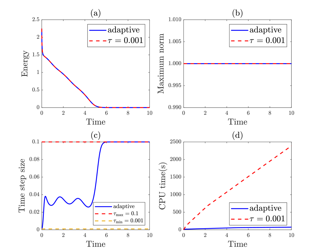
Figure 1: Example 1: (a) Evolution of energy with final time $T_{2}=10$. (b) Evolution of maximum norm with final time $T_{2}=10$. (c) Evolution of time step size with final time $T_{2}=10$. (d) Evolution of CPU cost time with final time $T_{2}=10$.

Example 2.

We consider the Allen–Cahn equation with logarithmic potential, i.e.,

(120) $$\partial_{t}u=\varepsilon^{2}\Delta u+\theta_{c}u-\frac{\theta}{2}(\ln(1+u)-\ln(1-u)).$$

We take the initial condition as $u^{0}(x,y)=0.5\left(\chi\left(\left(x-\pi\right)^{2}+\left(y-\pi\right)^{2}\leq 1.2\right)-0.5\right).$ The other parameters are $\varepsilon=0.01$, $\theta_{c}=1$ and $\theta=\frac{1}{4}$ as in [36].

The Strang splitting method can be written as

(121) $$u^{n+1}=\mathcal{S}_{\mathcal{L}}\left(\frac{\tau_{n+1}}{2}\right)\mathcal{S}_{\mathcal{N}}^{(\text{LOG})}(\tau_{n+1})\mathcal{S}_{\mathcal{L}}\left(\frac{\tau_{n+1}}{2}\right)u^{n},$$

where Runge–Kutta formulae is applied in approximating $\mathcal{S}_{\mathcal{N}}^{(\text{LOG})}(\tau_{n+1})$. The Butcher tableau is written as

(122) $$\begin{array}[]{c|cc}a&a&0\\ 1-a&1-2a&a\\ \hline\cr&\frac{1}{2}&\frac{1}{2}\end{array}$$

with $a=1+\frac{\sqrt{2}}{2}$. We use $512\times 512$ Fourier modes for the space discretization. The homogeneous Neumann boundary condition is employed. First, we show the $H^{1}$-norm errors of the numerical solution at $T_{1}=1$ using (117). Table 2 shows that the convergence order is about 2. Next, a numerical experiment with $512\times 512$ Fourier modes up to $T_{2}=10$ is carried out. We choose $\tau_{\min}=0.001$, $\tau_{\max}=0.01$ and $\alpha=100$ to calculate the solution $u_{\text{num}}$ with the same adaptive strategy (118). We also calculate the “reference” solution $u_{\text{ref}}$ with time step $\tau=0.001$. In Fig. 2, the $L^{\infty}$-norm of the numerical solutions remains bounded, and the energy dissipates over time. In Fig. 2(d), the CPU cost of adaptive strategy is much less than that of the uniform-time-step strategy. By (119), the relative error is about $5.1\times 10^{-5}$. It indicates that the adaptive strategy is almost as accurate as the uniform-time-step strategy, but more efficient.

Table 2: Example 2: $H^{1}$-norm errors of numerical solutions at time $T_{2}=1$ for Allen–Cahn equation with logarithmic potential.

 

$N$	$100$	$200$	$400$	$800$	$1600$
$H^{1}$-error	$1.300\times 10^{-3}$	$3.228\times 10^{-4}$	$7.240\times 10^{-5}$	$1.796\times 10^{-5}$	$4.468\times 10^{-6}$
rate	–	$2.0002$	$2.0189$	$2.0331$	$2.0211$

 

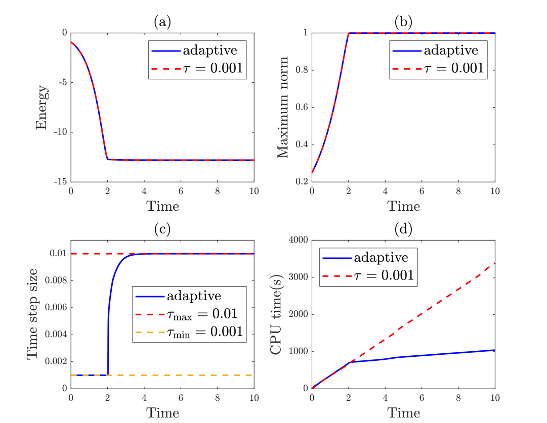
Figure 2: Example 2: (a) Evolution of energy with final time $T_{2}=10$. (b) Evolution of maximum norm with final time $T_{2}=10$. (c) Evolution of CPU cost with final time $T_{2}=10$. (d) Evolution of time step size with final time $T_{2}=10$.

Example 3.

Consider the ternary conservative Allen–Cahn equations:

(123) $$\partial_{t}u_{l}=\varepsilon^{2}\Delta u_{l}-\left(f\left(u_{l}\right)-\beta\left(u_{l}\right)+\Lambda\left(u_{1},u_{2},u_{3}\right)\right)\quad\text{ in }\Omega\times(0,T],\quad l=1,2,3\text{, }$$

where $F\left(u_{l}\right)=\frac{1}{2}u_{l}^{2}\left(1-u_{l}\right)^{2},f\left(u_{l}\right)=F^{\prime}\left(u_{l}\right)$ and $\varepsilon=0.05$. $\beta(u)$ and $\Lambda\left(u_{1},u_{2},u_{3}\right)$ are defined as

(124) $$\beta(u_{l}) =\frac{1}{\left|\Omega\right|}\int_{\Omega}F^{\prime}(u_{l})\,{\mathrm{d}}x,\quad l=1,2,3,\quad\Lambda\left(u_{1},u_{2},u_{3}\right)=-\frac{1}{3}\sum_{l=1}^{3}\left(f\left(u_{l}\right)-\beta\left(u_{l}\right)\right).$$

The energy functional can be written as $E(u_{1},u_{2},u_{3})=\sum_{l=1}^{3}\int_{\Omega}\left(\frac{\varepsilon^{2}}{2}\left|\nabla u_{l}\right|^{2}+F(u_{l})\right)\,{\mathrm{d}}x.$ We take the following initial conditions

(125) $$\left\{\begin{array}[]{l}\phi_{l}(x)=\operatorname{rand}(x),\\ u_{l}^{0}(x)=\frac{\phi_{l}(x)}{\phi_{1}(x)+\phi_{2}(x)+\phi_{3}(x)},\end{array}\right.$$

where $l=1,2,3$ and $\operatorname{rand}(\cdot)$ is the uniformly distributed random function.

Here, the nonlinear operator ${\mathcal{S}_{\mathcal{N}}}(\tau)(u_{1},u_{2},u_{3})$ is approximated using the Runge–Kutta formula (as in [52]). The first equation in (124) guarantees the mass conservation of each component and the second equation ensures the hyperplane link $u_{1}+u_{2}+u_{3}=1$.

We use $128\times 128$ Fourier modes for the space discretization. The periodic boundary condition is employed. We choose $\tau_{\min}=0.001$, $\tau_{\max}=0.1$ and $\alpha=100$ to calculate the numerical solution. In Fig. 3, the equilibrium solution exhibits a regular shape with the contact angles of about $\frac{2}{3}\pi$. The evolution of time step size and original energy is displayed in Fig. 4. We can see that the original energy is dissipating over time.

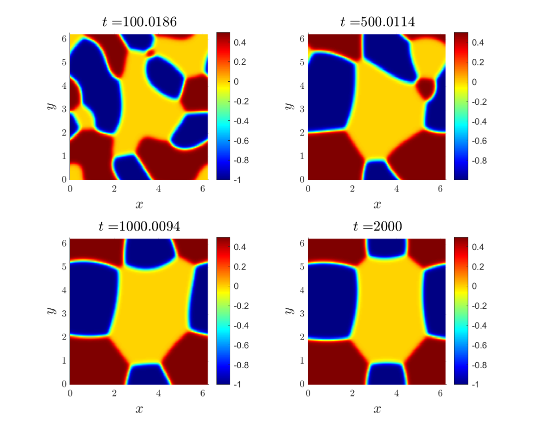
Figure 3: Example 3: Snapshots of $\frac{1}{2}u_{1}-u_{2}$ at $t=100.0186,500.0114,1000.0094,2000$ using adaptive time-stepping strategy (118).

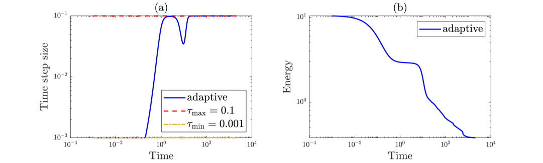
Figure 4: Example 3: (a) Evolution of time step size (in log scale) with final time $T=2000$. (b) Evolution of energy (in log scale) with final time $T=2000$.

6 Conclusions

In this article, we consider to solve the Allen–Cahn equation with homogeneous Neumann boundary condtion by the Strang splitting method with variable time steps. We establish the $H^{k}$-norm stability of Strang splitting method for the Allen–Cahn equation with polynomial potential. Furthermore, rigorous $H^{k}$-norm convergence analysis are given, under the initial regularity assumptions $u^{0}\in H^{k+6}(\Omega)$. Numerical simulations show the convergence rate, energy dissipation law and the efficiency of the adaptive time-stepping strategy.

Data Availibility

Data will be made available on reasonable request.

References

- [1] G. Akrivis, B. Li, and D. Li, Energy-decaying extrapolated RK–SAV methods for the Allen–Cahn and Cahn–Hilliard equations, SIAM J. Sci. Comput., 41 (2019), pp. A3703–A3727.
- [2] S. M. Allen and J. W. Cahn, A microscopic theory for antiphase boundary motion and its application to antiphase domain coarsening, Acta Metallurgica, 27 (1979), pp. 1085–1095.
- [3] P. Bader and S. Blanes, Fourier methods for the perturbed harmonic oscillator in linear and nonlinear Schrödinger equations, Physical Review E, 83 (2011), p. 046711.
- [4] W. Bao, Y. Cai, and Y. Feng, Improved uniform error bounds of the time-splitting methods for the long-time (nonlinear) Schrödinger equation, Mathematics of Computation, 92 (2023), pp. 1109–1139.
- [5] W. Bao, Y. Cai, and J. Yin, Super-resolution of time-splitting methods for the Dirac equation in the nonrelativistic regime, Mathematics of Computation, 89 (2020), pp. 2141–2173.
- [6] W. Bao, Y. Feng, and C. Su, Uniform error bounds of time-splitting spectral methods for the long-time dynamics of the nonlinear Klein–Gordon equation with weak nonlinearity, Mathematics of Computation, 91 (2022), pp. 811–842.
- [7] W. Bao and J. Shen, A fourth-order time-splitting Laguerre–Hermite pseudospectral method for Bose–Einstein condensates, SIAM Journal on Scientific Computing, 26 (2005), pp. 2010–2028.
- [8] A. Behzadan and M. Holst, Multiplication in sobolev spaces, revisited, Arkiv för Matematik, 59 (2021), pp. 275–306.
- [9] J. Bernier, Exact splitting methods for semigroups generated by inhomogeneous quadratic differential operators, Foundations of Computational Mathematics, 21 (2021), pp. 1401–1439.
- [10] S. Blanes and C. J. Budd, Adaptive geometric integrators for Hamiltonian problems with approximate scale invariance, SIAM Journal on Scientific Computing, 26 (2005), pp. 1089–1113.
- [11] S. Blanes, F. Casas, C. Gonzalez, and M. Thalhammer, Splitting methods with complex coefficients for linear and nonlinear evolution equations, arXiv preprint arXiv:2410.13011, (2024).
- [12] S. Blanes, F. Casas, and A. Murua, Splitting methods for differential equations, Acta Numerica, 33 (2024), p. 1–161.
- [13] S. Blanes and V. Gradinaru, High order efficient splittings for the semiclassical time-dependent Schrödinger equation, Journal of Computational Physics, 405 (2020), p. 109157.
- [14] S. Blanes and A. Iserles, Explicit adaptive symplectic integrators for solving Hamiltonian systems, Celestial Mechanics and Dynamical Astronomy, 114 (2012), pp. 297–317.
- [15] H. Brezis and H. Brézis, Functional analysis, Sobolev spaces and partial differential equations, vol. 2, Springer, 2011.
- [16] L. Q. Chen and J. Shen, Applications of semi-implicit fourier-spectral method to phase field equations, Comput. Phys. Commun., 108 (1998), pp. 147–158.
- [17] W. Chen, X. Wang, Y. Yan, and Z. Zhang, A second order BDF numerical scheme with variable steps for the Cahn–Hilliard equation, SIAM Journal on Numerical Analysis, 57 (2019), pp. 495–525.
- [18] Y. Cheng, A. Kurganov, Z. Qu, and T. Tang, Fast and stable explicit operator splitting methods for phase-field models, J. Comput. Phys., 303 (2015), pp. 45–65.
- [19] Q. Du, L. Ju, X. Li, and Z. Qiao, Maximum principle preserving exponential time differencing schemes for the nonlocal Allen–Cahn equation, SIAM J. Numer. Anal., 57 (2019), pp. 875–898.
- [20] Q. Du, L. Ju, X. Li, and Z. Qiao, Maximum bound principles for a class of semilinear parabolic equations and exponential time-differencing schemes, SIAM Review, 63 (2021), pp. 317–359.
- [21] L. C. Evans, Partial differential equations, vol. 19, American Mathematical Society, 2022.
- [22] Z. Fu, J. Shen, and J. Yang, Higher-order energy-decreasing exponential time differencing runge-kutta methods for gradient flows, Sci. China Math., (2024).
- [23] Z. Fu, T. Tang, and J. Yang, Unconditionally energy decreasing high-order Implicit-Explicit Runge-Kutta methods for phase-field models with the Lipschitz nonlinearity, Math. Comp., (2024).
- [24] Z. Fu and J. Yang, Energy-decreasing exponential time differencing Runge–Kutta methods for phase-field models, J. Comput. Phys., 454 (2022), p. 110943.
- [25] R. Glowinski, S. Leung, and J. Qian, A simple explicit operator-splitting method for effective Hamiltonians, SIAM Journal on Scientific Computing, 40 (2018), pp. A484–A503.
- [26] H. Gomez and T. J. Hughes, Provably unconditionally stable, second-order time-accurate, mixed variational methods for phase-field models, Journal of Computational Physics, 230 (2011), pp. 5310–5327.
- [27] E. Hairer, C. Lubich, and G. Wanner, Geometric numerical integration illustrated by the Störmer–Verlet method, Acta Numerica, 12 (2003), pp. 399–450.
- [28] E. Hairer, G. Wanner, and C. Lubich, Structure-Preserving Implementation, Springer Berlin Heidelberg, Berlin, Heidelberg, 2006, pp. 303–336.
- [29] M. Hochbruck and A. Ostermann, Exponential integrators, Acta Numerica, 19 (2010), pp. 209–286.
- [30] D. Hou, L. Ju, and Z. Qiao, A linear second-order maximum bound principle-preserving BDF scheme for the Allen–Cahn equation with a general mobility, Mathematics of Computation, 92 (2023), pp. 2515–2542.
- [31] Y. Huang, W. Yang, H. Wang, and J. Cui, Adaptive operator splitting finite element method for Allen–Cahn equation, Numerical Methods for Partial Differential Equations, 35 (2019), pp. 1290–1300.
- [32] T. Jahnke and C. Lubich, Error bounds for exponential operator splittings, BIT Numerical Mathematics, 40 (2000), pp. 735–744.
- [33] L. Ju, X. Li, Z. Qiao, and J. Yang, Maximum bound principle preserving integrating factor Runge–Kutta methods for semilinear parabolic equations, J. Comput. Phys., 439 (2021), p. 110405.
- [34] L. Ju, J. Zhang, L. Zhu, and Q. Du, Fast explicit integration factor methods for semilinear parabolic equations, Journal of Scientific Computing, 62 (2015), pp. 431–455.
- [35] R. Lan, J. Li, Y. Cai, and L. Ju, Operator splitting based structure-preserving numerical schemes for the mass-conserving convective Allen–Cahn equation, Journal of Computational Physics, 472 (2023), p. 111695.
- [36] D. Li, C. Quan, and J. Xu, Stability and convergence of Strang splitting. Part I: Scalar Allen–Cahn equation, Journal of Computational Physics, 458 (2022), p. 111087.
- [37] D. Li, C. Quan, and J. Xu, Stability and convergence of Strang splitting. Part II: Tensorial Allen–Cahn equations, Journal of Computational Physics, 454 (2022), p. 110985.
- [38] J. Li, L. Ju, Y. Cai, and X. Feng, Unconditionally maximum bound principle preserving linear schemes for the conservative Allen–Cahn equation with nonlocal constraint, J. Sci. Comput., 87 (2021), pp. 1–32.
- [39] J. Li, X. Li, L. Ju, and X. Feng, Stabilized integrating factor Runge–Kutta method and unconditional preservation of maximum bound principle, SIAM J. Sci. Comput., 43 (2021), pp. A1780–A1802.
- [40] X. Li, Z. Qiao, and H. Zhang, Convergence of a fast explicit operator splitting method for the epitaxial growth model with slope selection, SIAM J. Numer. Anal., 55 (2017), pp. 265–285.
- [41] H. Liao, T. Tang, and T. Zhou, On energy stable, maximum-principle preserving, second-order BDF scheme with variable steps for the Allen–-Cahn equation, SIAM Journal on Numerical Analysis, 58 (2020), pp. 2294–2314.
- [42] H. Liao and Z. Zhang, Analysis of adaptive BDF2 scheme for diffusion equations, Mathematics of Computation, 90 (2021), pp. 1207–1226.
- [43] C. Liu, C. Wang, and Y. Wang, A structure-preserving, operator splitting scheme for reaction-diffusion equations with detailed balance, Journal of Computational Physics, 436 (2021), p. 110253.
- [44] C. Liu, C. Wang, Y. Wang, and S. M. Wise, Convergence analysis of the variational operator splitting scheme for a reaction-diffusion system with detailed balance, SIAM Journal on Numerical Analysis, 60 (2022), pp. 781–803.
- [45] R. I. McLachlan and G. R. W. Quispel, Splitting methods, Acta Numerica, 11 (2002), pp. 341–434.
- [46] Z. Qiao, Z. Zhang, and T. Tang, An adaptive time-stepping strategy for the molecular beam epitaxy models, SIAM Journal on Scientific Computing, 33 (2011), pp. 1395–1414.
- [47] M. Reed and B. Simon, Methods of modern mathematical physics: Functional analysis, vol. 1, Gulf Professional Publishing, 1980.
- [48] J. Shen, T. Tang, and J. Yang, On the maximum principle preserving schemes for the generalized Allen–Cahn equation, Commun. Math. Sci., 14 (2016), pp. 1517–1534.
- [49] J. Shen, J. Xu, and J. Yang, The scalar auxiliary variable (SAV) approach for gradient flows, J. Comput. Phys., 353 (2018), pp. 407–416.
- [50] G. Strang, On the construction and comparison of difference schemes, SIAM Journal on Numerical Analysis, 5 (1968), pp. 506–517. Publisher: SIAM.
- [51] T. Tang and J. Yang, Implicit-explicit scheme for the Allen-Cahn equation preserves the maximum principle, J. Comput. Math., (2016), pp. 451–461.
- [52] Z. Weng, S. Zhai, W. Dai, Y. Yang, and Y. Mo, Stability and error estimates of Strang splitting method for the nonlocal ternary conservative Allen–Cahn model, Journal of Computational and Applied Mathematics, 441 (2024), p. 115668.
- [53] X. Yang, Linear, first and second-order, unconditionally energy stable numerical schemes for the phase field model of homopolymer blends, J. Comput. Phys., 327 (2016), pp. 294–316.