Gravitational wave signals from primordial black holes orbiting solar-type stars

Abstract

Primordial black holes (PBHs) with masses between $10^{14}$ and $10^{20}$ kg are candidates to contribute a substantial fraction of the total dark matter abundance. When in orbit around the center of a star, which can possibly be a completely interior orbit, such objects would emit gravitational waves, as predicted by general relativity. In this work, we examine the gravitational wave signals emitted by such objects when they orbit typical stars, such as the Sun. We show that the magnitude of the waves that could eventually be detected on Earth from a possible PBH orbiting the Sun or a neighboring Sun-like star within our galaxy can be significantly stronger than those originating from a PBH orbiting a denser but more distant neutron star (NS). Such signals may be detectable by the LISA gravitational-wave detector. In addition, we estimate the contribution that a large collection of such PBH-star systems would make to the stochastic gravitational-wave background (SGWB) within a range of frequencies to which pulsar timing arrays are sensitive.

I Introduction

Primordial black holes (PBHs) are hypothetical black holes that could have formed in the very early universe, for example from the gravitational collapse of primordial perturbations that were amplified during a phase of inflation. Although no PBHs have been conclusively detected, they can act as a component of dark matter. The relevant constraints leave open a window of masses $10^{14}\,\text{kg}\leq m\leq 10^{20}\,\text{kg}$, often dubbed the “asteroid-mass range,” within which PBHs could constitute the entire dark matter abundance Carr and Kühnel (2020); Green and Kavanagh (2021); Carr et al. (2024); Escrivà et al. (2022); Gorton and Green (2024); Khlopov (2024).

The discovery of gravitational waves (GWs) has opened up an entirely new branch of astronomy. Since the first detection, there have been numerous other detections of GWs from black hole mergers and neutron star collisions, significantly enhancing our understanding of the universe Bailes et al. (2021). In this paper we study several scenarios in which PBHs within the asteroid-mass range could yield observable GW signals.

Typically when possible GW signals from asteroid-mass PBHs have been considered, the focus has been on primordial tensor perturbations induced at second order in perturbation theory from the large-amplitude scalar curvature perturbations that would have undergone gravitational collapse at very early times to yield a population of PBHs. The peak frequency of such primordial GWs depends on the typical mass $m$ with which the PBHs form; for PBHs in the asteroid-mass range, such induced GW signals today would peak in the range $f\sim{\cal O}(10^{0}-10^{3})\,\text{Hz}$, with predicted amplitudes to which upcoming GW detectors, such as the Einstein Telescope Abac et al. (2025) and Cosmic Explorer Reitze et al. (2019), should be sensitive. (See, e.g., Refs. Domènech (2021); Qin et al. (2023).)

In this paper we consider GWs arising from very different processes involving asteroid-mass PBHs, with correspondingly different frequencies and hence distinct opportunities for detection in upcoming detectors. In particular, we build upon previous work in which trajectories of small primordial black holes bound to stellar objects were studied in detail De Lorenci et al. (2024), and calculate the characteristic features of the GWs that such systems should emit. For a PBH of mass $m\simeq 10^{20}\,\text{kg}$ trapped in the Sun, we show that the resulting GWs from the PBH’s orbital motion should be detectable in future GW experiments such as LISA Seoane et al. (2023), since the very faint amplitude at emission would be compensated by the very short distance between our star and the detectors. (Compare with Refs. Baumgarte and Shapiro (2024a, b, c).)

In addition to considering the GW signals from single PBH-star systems, we also estimate the contribution that a large collection of such systems would make, integrated over cosmic history, to the stochastic gravitational-wave background (SGWB). Recent measurements of the SGWB using pulsar timing arrays are in tension with predictions of the signal that would arise from the presumed dominant contribution, namely, the binary inspiral of supermassive black holes Afzal et al. (2023). We find that a large collection of small-mass PBHs orbiting ordinary Sun-like stars would contribute to the SGWB and could help ease the present tension with observations.

In Section II we introduce our parameterization for the PBH-star systems, and in Section III we identify the dominant (quadrupole) contribution to the GW emission from such systems. We also identify appropriate time-scales within which our estimates remain self-consistent. Section IV presents results for individual GW waveforms resulting from a variety of PBH-star orbits, including those in which the PBH remains entirely bound within its host star. We then turn in Section V to study whether such individual-system GW signals might be detectable with upcoming GW experiments, such as LISA. In Section VI we estimate the expected contribution to the SGWB, including the likely spectral index from a large collection of such PBH-star systems over cosmic history. We present concluding remarks in Section VII.

II Dynamics of a PBH in a stellar orbit

Following the methodology in Ref. De Lorenci et al. (2024), we consider the dynamics of a PBH of mass $m$ in orbit around the center of a star of mass $M_{\star}$ and radius $R$. (See Fig. 1 for the geometric configuration discussed below.) The PBHs of interest have very small cross-sections, due to their asteroid-sized masses, so that their orbits can occur partially or even totally inside the star interior ($r<R$). In this case, the gravitational potential energy $U(r)$ of the PBH will depend on its radial position in such a way that

$$U(r)=\int_{+\infty}^{r}\frac{GmM(u)}{u^{2}}\text{d}u,$$ (1)

where

$$M(r)=\left\{\begin{array}[]{l}\displaystyle 4\pi\int_{0}^{r}\rho(v)v^{2}\text{d}v,\ \ r<R\\ M_{\star},\ \ r\geq R\end{array}\right.$$ (2)

represents the enclosed star mass that effectively interacts with the PBH when it is at a distance $r$ from the origin.

The motion of a particle under such a potential preserves its angular momentum $L=mr^{2}\dot{\varphi}\doteq m\ell$, and also its total energy $E_{\textsc{t}}=\frac{1}{2}m\dot{r}^{2}+\frac{1}{2}mr^{2}\dot{\varphi}^{2}+U(r)$, and $U(r)$ coincides with the Keplerian potential energy $U(r)=-GmM_{\star}/r$ when $r\geq R$, as expected.

The differential equation governing the orbital motion of a PBH can be conveniently written in terms of the dimensionless radial distance $s=r/R$ and time $\tau=\sqrt{GM_{\star}/R^{3}}\,t$ variables as

$$s^{\prime\prime}=\frac{\bar{\ell}^{2}}{s^{3}}-\frac{\bar{M}(s)}{s^{2}},$$ (3)

where a prime denotes a derivative with respect to $\tau$. The dimensionless mass function is defined through $\bar{M}(s)=M(s)/M_{\star}$, while the angular-momentum density is $\bar{\ell}=\ell/\sqrt{GM_{\star}R}$.

The angular distance between the apocenter $r_{\text{max}}$ and pericenter $r_{\text{min}}$ of the orbit is given by (see the discussion in the appendix of Ref. De Lorenci et al. (2024))

$$\delta\varphi=\int_{s_{\text{min}}}^{s_{\text{max}}}\frac{\bar{\ell}}{\sqrt{2\left[\bar{E}_{\textsc{t}}-\bar{V}(s)\right]}}\frac{\text{d}s}{s^{2}},$$ (4)

where $s_{\text{max}}=r_{\text{max}}/R$ and $s_{\text{min}}=r_{\text{max}}/R$ give the maximum and minimum distances from the particle’s orbit to the origin, $\bar{V}(s)$ is the dimensionless effective potential of the particle, defined through

$$\bar{V}(s)=\frac{\bar{\ell}^{2}}{2s^{2}}+\int_{+\infty}^{s}\frac{\bar{M}(u)}{u^{2}}\text{d}u,$$ (5)

and

$$E_{\textsc{t}}=\frac{GmM_{\star}}{R}\bar{E}_{\textsc{t}}=\frac{GmM_{\star}}{R}\left[\frac{1}{2}s^{\prime 2}+\bar{V}(s)\right],$$ (6)

is the dimensionless total energy of the particle.

As discussed in Ref. De Lorenci et al. (2024), the leading relativistic correction to the equation of motion for the PBH is given by $3GM(r)\ell^{2}/(r^{4}c^{2})$. The ratio of this term to the Newtonian $GM(r)/r^{2}$ term is $3(\ell/cr)^{2}$, which is found to remain below $\mathcal{O}(10^{-5})$ for the orbital motions under study here; hence we can safely neglect post-Newtonian corrections over the time-scales of interest. Likewise, dynamical friction for such systems typically scales as $t_{\text{dyn}}\simeq 10^{-1}(M/m)\,t_{\text{orbit}}$, where $t_{\text{orbit}}\sim R/v_{0}$ Ostriker (1999); Baumgarte and Shapiro (2024b); Caiozzo et al. (2024). For $M_{\star}\sim M_{\odot}$, $R\sim R_{\odot}$, and $v_{0}\sim{\cal O}(10^{2})\,\text{km}\,\text{s}^{-1}$, this suggests that dynamical friction should affect the PBH’s orbit on a time-scale $10^{6}\,\text{yr}\leq t_{\text{dyn}}\leq 10^{12}\,\text{yr}$ for PBH masses within the range $10^{14}\,\text{kg}\leq m\leq 10^{20}\,\text{kg}$, many order of magnitude longer than the typical orbital time $t_{\text{orbit}}\sim 10^{4}\,\text{s}$. We therefore also neglect dynamical friction over the relevant time-scales for our calculations.

III Gravitational waves

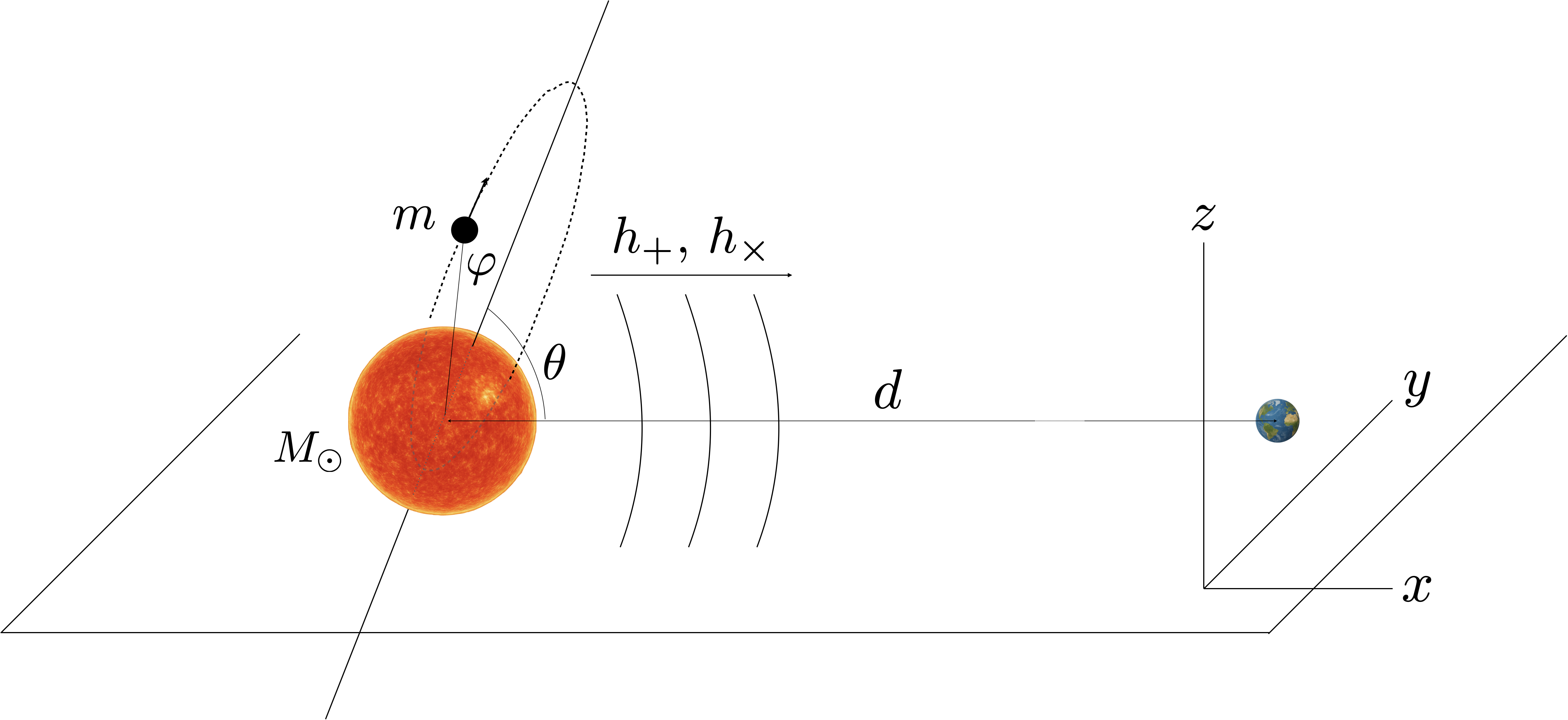
Figure 1: Illustration for the Sun-Earth example of the geometric configuration for the emission of gravitational waves with polarizations $h_{+}$ and $h_{\times}$. The trajectory of the mass $m$ orbiting the mass $M_{\odot}\gg m$ lies entirely in a plane making an angle $\theta$ with the ecliptic plane. In the best-case scenario, one has $\theta=\pi/2$ so the PBH remains in the $y-z$ plane, with GW emission along the $x-$direction.

For the parameter ranges of interest, the system we study falls within a weak gravitational regime. In that case, the gravitational waves will be dominated by the quadrupole moment. The next-leading correction beyond quadrupole is the first post-Newtonian (PN) contribution, which is expected to be of order ${\cal O}(v^{2}/c^{2})$. In the small-velocity regime considered here, this term introduces only a minor correction that remains negligible over the time-scale relevant to our analysis. In that case, the transverse-traceless (TT) component of the gravitational wave strain tensor takes the form Shapiro and Teukolsky (1986)

$$h_{ij}^{\textsc{tt}}=\frac{2G}{c^{4}d}\perp_{ijk\ell}\ddot{\mathrel{\vbox{\offinterlineskip\hbox{$I$}\vskip-3.87495pt\hbox{\scalebox{0.9}{--}}}}}_{k\ell},$$ (7)

where $d$ is the distance between the source and the observer and $\mathrel{\vbox{\offinterlineskip\hbox{$I$}\vskip-3.87495pt\hbox{\scalebox{0.9}{--}}}}_{ij}$ denotes the traceless part of the mass quadrupole moment tensor of the source,

$$\mathrel{\vbox{\offinterlineskip\hbox{$I$}\vskip-3.87495pt\hbox{\scalebox{0.9}{--}}}}_{jk}=m\left(x_{j}x_{k}-\frac{1}{3}\bm{x}^{2}\delta_{jk}\right),$$ (8)

with $x_{i}$ the $i$th component of the position of the PBH in its planar orbital motion and $\bm{x}^{2}=\delta^{ij}x_{i}x_{j}$. In Eq. (7), the projector $\perp_{ijk\ell}$ along the unit vector $n_{i}$ is given by

$$\perp_{ijk\ell}=\perp_{(ik}\perp_{j)\ell}-\frac{1}{2}\perp_{ij}\perp_{k\ell},$$ (9)

with $\perp_{ij}=\delta_{ij}-n_{i}n_{j}$, and the symmetrization is only in $i$ and $j$.

We neglect the effect of time retardation, as our interest lies only in the magnitude of the emitted gravitational radiation. This approximation simplifies the analysis but at the cost of losing precise information about the timing and relative phase of the gravitational waves, which could be significant, for instance, when the source is rapidly changing or located far from the observer. However, the influence of the retardation effect for periodic or quasi-periodic orbits is generally less important, as the regular pattern of the emission enables one to determine the frequency and amplitude of the waves, which are the main physical characteristics of the radiation Thorne (1980).

With respect to the dimensionless variables, defined by $\bar{x}_{i}=x_{i}/R$, the orbit of the PBH has the form, in the reference frame defined in Fig. 1,

$$(\bar{x},\bar{y},\bar{z})=s(t)\left\{\cos\theta,\cos\left[\varphi(t)\right]\sin\theta,\sin\left[\varphi(t)\right]\sin\theta\right\},$$ (10)

where $\theta$ is a constant indicating the overall inclination of the PBH trajectory with respect to the ecliptic plane. From now on, and for the sake of simplicity, we shall assume $\theta\to\pi/2$, thereby maximizing the observed GW. For an arbitrarily inclined trajectory, it suffices to put back the relevant factor $\cos^{2}\theta$ in the final results. Under these simplifying assumptions, the quadrupole moment of Eq. (8) takes the form

$$\mathrel{\vbox{\offinterlineskip\hbox{$I$}\vskip-3.87495pt\hbox{\scalebox{0.9}{--}}}}_{k\ell}=mR^{2}\left(\bar{x}_{k}\bar{x}_{\ell}-\frac{1}{3}\delta_{k\ell}s^{2}\right)\doteq mR^{2}\bar{\mathrel{\vbox{\offinterlineskip\hbox{$I$}\vskip-3.87495pt\hbox{\scalebox{0.9}{--}}}}}_{k\ell}.$$ (11)

Finally, using the dimensionless time variable $\tau$, the strain tensor of Eq. (7) becomes

$$h_{ij}^{\textsc{tt}}=\frac{2G^{2}mM_{\star}}{c^{4}Rd}\,\perp_{ijk\ell}\bar{\mathrel{\vbox{\offinterlineskip\hbox{$I$}\vskip-3.87495pt\hbox{\scalebox{0.9}{--}}}}}^{\prime\prime}_{k\ell}\doteq h_{+}\varepsilon_{ij}^{+}+h_{\times}\varepsilon_{ij}^{\times},$$ (12)

in which the polarization tensors have nonvanishing components only in the $y-z$ directions, reading $\varepsilon^{+}=\sigma_{z}$ and $\varepsilon^{\times}=\sigma_{x}$ in terms of the Pauli matrices. Notice that the prefactor in Eq. (12) is a number that characterizes the physical properties of the system, including its distance from the observer, while the geometric part $\bar{\mathrel{\vbox{\offinterlineskip\hbox{$I$}\vskip-3.87495pt\hbox{\scalebox{0.9}{--}}}}}^{\prime\prime}_{ij}$ also includes the time dependence. Explicitly, the modes are given by

$$h_{+}= \frac{2G^{2}mM_{\star}}{c^{4}Rd}\,\left\{\alpha(\tau)\cos[2\varphi(\tau)]-\beta(\tau)\sin[2\varphi(\tau)]\right\}$$

$$\doteq \left(\frac{2G^{2}mM_{\star}}{c^{4}Rd}\right)\bar{h}_{+}\,,$$ (13)

$$h_{\times}= \frac{2G^{2}mM_{\star}}{c^{4}Rd}\,\left\{\alpha(\tau)\sin[2\varphi(\tau)]+\beta(\tau)\cos[2\varphi(\tau)]\right\}$$

$$\doteq \left(\frac{2G^{2}mM_{\star}}{c^{4}Rd}\right)\bar{h}_{\times}\,,$$ (14)

where we introduced the notation for the scaled strains $\bar{h}_{+}$ and $\bar{h}_{\times}$, and defined

$$\alpha(\tau) =s^{\prime 2}+ss^{\prime\prime}-2s^{2}\varphi^{\prime 2}=s^{\prime 2}-\frac{\bar{\ell}^{2}}{s^{2}}-\frac{\bar{M}(s)}{s},$$ (15)

$$\beta(\tau) =s^{2}\left(\varphi^{\prime\prime}+4\frac{s^{\prime}}{s}\varphi^{\prime}\right)=2\frac{\bar{\ell}s^{\prime}}{s},$$ (16)

so that the resulting $l=2$ multipole amplitude reads

$$h^{\textsc{tt}}(\tau)\doteq\sqrt{h_{+}^{2}+h_{\times}^{2}}=\frac{2G^{2}mM_{\star}}{c^{4}Rd}\,\sqrt{\alpha^{2}+\beta^{2}}.$$ (17)

	distance ($d$/km)	Mass ($M_{\star}$/kg)	Radius ($R$/km)
Sun	$1.496\times 10^{8}$	$M_{\odot}$	$6.957\times 10^{5}$
Vela	$9.072\times 10^{15}$	$1.4M_{\odot}$	9.656

Table 1: Sizes and distances from Earth of our Sun and the Vela pulsar.

For the sake of comparison and future reference, we consider a PBH of mass $m$ orbiting either our Sun or the Vela pulsar, with the relevant physical parameters gathered in Table 1. Substituting these quantities into Eq. (12), it is evident that for PBHs of identical masses, the ratio of the GW amplitudes emitted by the Sun-PBH system compared to the Vela-PBH system, as observed on Earth, is approximately $600$. Hence, the same orbit of a PBH around the Sun would emit GW radiation that, when measured on Earth, would be approximately 600 times more intense than the radiation originating from Vela. This large ratio is interesting given the prevalence of Sun-like stars within our astronomical neighborhood.

We remark that if two stars have the same mass distribution, then PBH orbits with the same (dimensionless) energy $\bar{E}_{T}$ and angular momentum $\bar{\ell}$ generate exactly the same pattern of gravitational radiation from the term $\bar{\mathrel{\vbox{\offinterlineskip\hbox{$I$}\vskip-3.87495pt\hbox{\scalebox{0.9}{--}}}}}^{\prime\prime}_{ij}$ in Eq. (12). Therefore the amplitude given by the coefficient in Eq. (12) provides the most important piece of information concerning the intensity of the emitted radiation.

Lastly, we note that the energy lost by the system due to the emission of gravitational waves (within the same quadrupole approximation) is given by Shapiro and Teukolsky (1986); Maggiore (2007)

$$\frac{\text{d}E}{\text{d}t}=-\sum_{ij}\frac{G}{5c^{5}}\left(\frac{\text{d}^{3}\!\!\mathrel{\vbox{\offinterlineskip\hbox{$I$}\vskip-3.87495pt\hbox{\scalebox{0.9}{--}}}}_{ij}}{\text{d}t^{3}}\right)^{2}.$$ (18)

As we will see, for the systems of interest here, the gravitational radiation spectrum is strongly peaked at a frequency $f_{\text{peak}}\simeq v_{0}/R$, with $v_{0}\lesssim v_{\text{esc}}=\sqrt{2GM_{\star}/R}$, or $f_{\text{peak}}^{2}\simeq 2GM_{\star}/R^{3}$. We may then approximate $\dot{h}^{\textsc{tt}}_{ij}\simeq i(2\pi f_{\text{peak}})h_{ij}^{\textsc{tt}}$, and, upon using Eqs. (7) and (18),

$$\bigg{|}\frac{\text{d}E}{\text{d}t}\bigg{|}\simeq\frac{4\pi^{2}}{5}\frac{c^{3}d^{2}M_{\star}}{R^{3}}\big{|}h^{\textsc{tt}}\big{|}^{2}.$$ (19)

The time-scale $t_{\text{gw}}$ over which energy loss due to emitted gravitational radiation would back-react on the PBH orbit is set by $E_{\text{grav}}/t_{\text{gw}}\simeq|\text{d}E/\text{d}t|$, where $E_{\text{grav}}=GmM_{\star}/R$, which yields

$$t_{\text{gw}}\simeq\frac{5}{4\pi^{2}}\frac{GmR^{2}}{c^{3}d^{2}}\frac{1}{|h^{\textsc{tt}}|^{2}}.$$ (20)

For fiducial values ($m=10^{20}\,\text{kg},M_{\star}=M_{\odot},R=R_{\odot},d=1.5\times 10^{8}\,\text{km}=1\,\text{AU}$), and using our estimate for $h^{\textsc{tt}}$ below, in Eq. (IV), we then find $t_{\text{gw}}\sim 10^{24}\,\text{s}$ for cases of interest here. Given $t_{\text{orbit}}\sim 10^{4}\,\text{s}$ and $t_{\text{dyn}}\sim 10^{13}\,\text{s}$ for these same fiducial parameters, we thus confirm the strict hierarchy

$$t_{\text{orbit}}\ll t_{\text{dyn}}\ll t_{\text{gw}}$$ (21)

for the PBH-star systems we are interested in. Hence we will neglect both dynamical friction and energy loss from gravitational radiation in what follows.

IV Simulations

Let us now investigate the GW pattern emitted by a PBH in a bound orbit around a typical star, like our Sun. For the sake of simplicity, we will adopt an idealized model De Lorenci et al. (2024) describing the mass-density profile of the star $\rho(r)$ given by

$$\rho(r)=\rho(0)\left(1-\frac{r}{R}\right)^{6}\Theta\left(1-\frac{r}{R}\right),$$ (22)

where $\rho(0)=1.184\times 10^{5}\,\text{kg}\,\text{m}^{-3}$, and $\Theta(x)$ is the Heaviside step function, defined as $\Theta(x)=1$ when $x>0$, $\Theta(0)=\frac{1}{2}$, and $\Theta(x)=0$ when $x<0$. The value for $\rho(0)$ is then chosen such that the total mass of the star coincides with the Sun’s mass. For the purposes of our discussion, this simple model describes the behavior of typical stars sufficiently well. (See Ref. De Lorenci et al. (2024) for further details.) The mass function $M(r)$ introduced in the last section can now be directly obtained by integrating $\rho(r)$ and is depicted in Fig. 2.

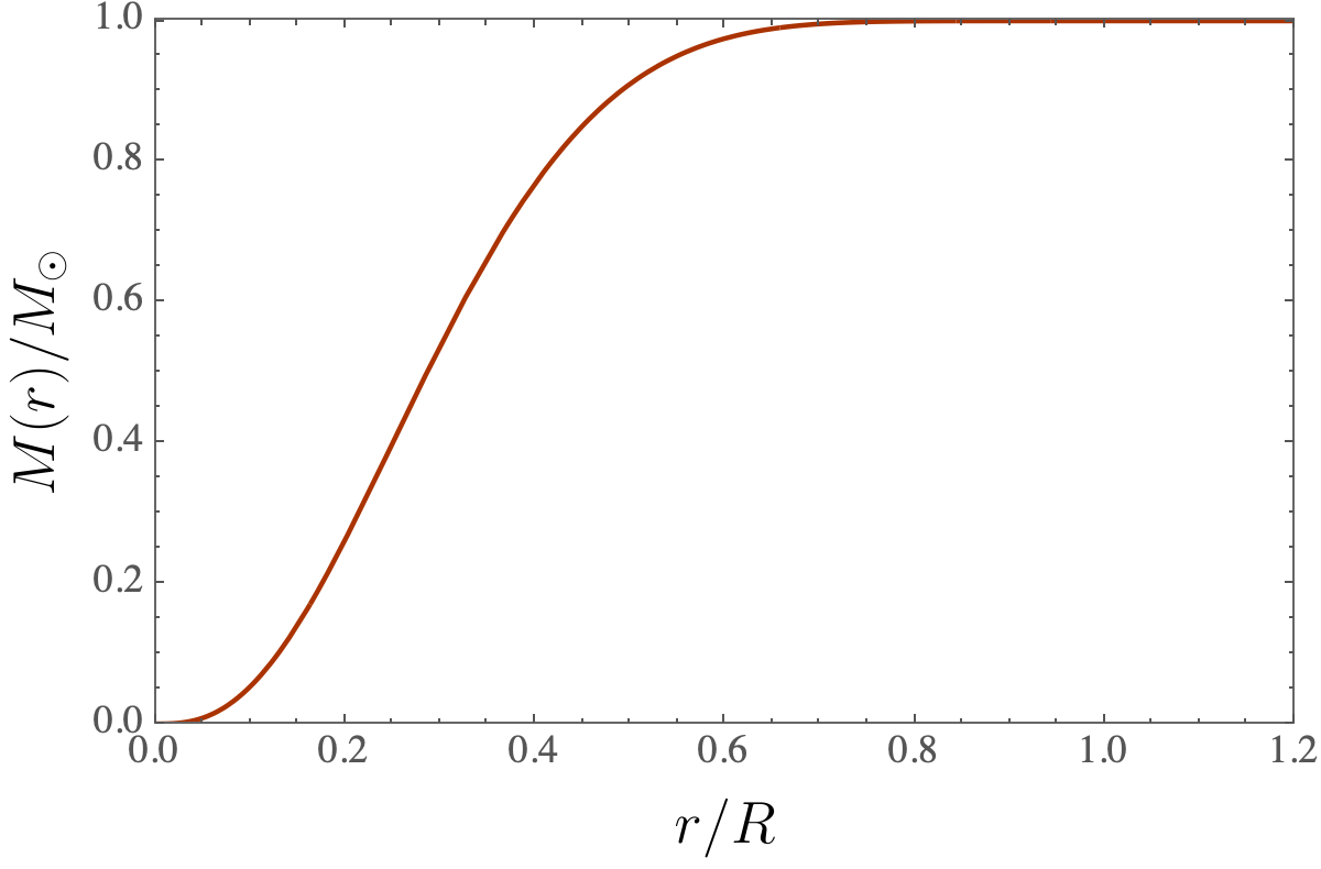
Figure 2: The normalized mass of the star, as determined from the idealized model given by $\rho(r)$ in Eq. (22).

The graph displayed in Fig. 3 is constructed by finding, for each $0<\bar{\ell}<1$, the smallest root of the equation

$$\bar{V}(s)=\frac{\bar{\ell}^{2}}{2s^{2}}+\int_{+\infty}^{s}\frac{\bar{M}(u)}{u^{2}}\text{d}u=\bar{V}(s_{0}),$$ (23)

i.e., the minimum distance of the orbit that starts at $s=s_{0}$ with zero radial velocity. The value of scaled strain $\bar{h}_{+}$ at this point is then computed, assuming it is aligned with the $x$-axis. This value coincides with the maximum values of $\bar{h}_{+}$ and $\bar{h}_{\times}$ across all orbits with the same fixed angular momentum and energies within the range $\bar{V}_{\text{min}}\leq\bar{E}_{\textsc{t}}\leq\bar{V}(s_{0})$.

Figure 3: Maximum amplitude of the gravitational wave signals emitted by the system, $h_{+}$ and $h_{\times}$, as a function of $\bar{\ell}$, for some representative values of $s_{0}$.

This maximum value of $\bar{h}_{+}$ is obtained by means of

$$\alpha=\frac{\bar{\ell}^{2}}{s^{2}}+\frac{\bar{M}(s)}{s},$$ (24)

where $s$ is taken as the minimum distance of the orbit to the center of the star, as explained above, and is also a function of $\bar{\ell}$.

In Fig. 4 the potential energy of the PBH is shown as a function of the distance $r$ for selected initial conditions. In particular, the dimensionless angular momentum per unit mass was chosen to be $\bar{\ell}=0.141$, from which, using the data for the Sun ($M_{\odot}=1.989\times 10^{30}\,\text{kg}$), it follows that $\ell=4.28\times 10^{13}\,\text{m}^{2}\text{s}^{-1}$. The shaded gradient region represents the density of the mass profile function described by Eq. (22).

Figure 4: The effective potential energy of the PBH as a function of $s=r/R$, where $R$ is the radius of the star. Here we assumed an angular momentum per unit mass such that $\bar{\ell}=0.1410$. The three horizontal lines indicate orbits with three distinct values of the total energy. The dotted horizontal line (with $\bar{E}_{\textsc{t}}>-1$ ) corresponds to a hybrid orbit, while the other two horizontal lines are associated with inner orbits.

Three possible values for the energy of the particle are also represented (the horizontal lines), corresponding to orbits with different initial conditions. The solid line near the bottom of the effective potential is associated with an orbit such that the total energy of the particle is given by $\bar{E}_{\textsc{t}}=-3.1678$ ($E_{\textsc{t}}=-6.0452\times 10^{31}\,\text{J}$ for a PBH of $10^{20}\,\text{kg}$). The dashed line corresponds to an orbit that achieves the maximum and minimum distances from the center of attraction at $r=0.39856\,R$ and $r=0.070740\,R$, respectively, where the corresponding speeds are approximately $v\approx 154.51\,\text{km}\,\text{s}^{-1}$ and $v\approx 870.54\,\text{km}\,\text{s}^{-1}$. Higher than $\bar{E}_{\textsc{t}}=-1$ values of energy would lead to orbit solutions that advance to the exterior region ($r>R$), as the one depicted by the dotted straight line, that achieves a maximum distance from the center at $r=1.7229\,R$. In this solution the particle speed at perihelion is $v\approx 357.43\,\text{km}\,\text{s}^{-1}$ while at the aphelion it achieves $v\approx 1,208.7\,\text{km}\,\text{s}^{-1}$.

The trajectories for the three solutions discussed in Fig. 4 are shown in the top panels of Figs. 5, 6 and 7. Notice that the least eccentric orbit corresponds to the solution with the smallest total energy, as could have been anticipated by examining Fig. 4. The initial conditions were chosen in such a way to produce closed orbits De Lorenci et al. (2024).

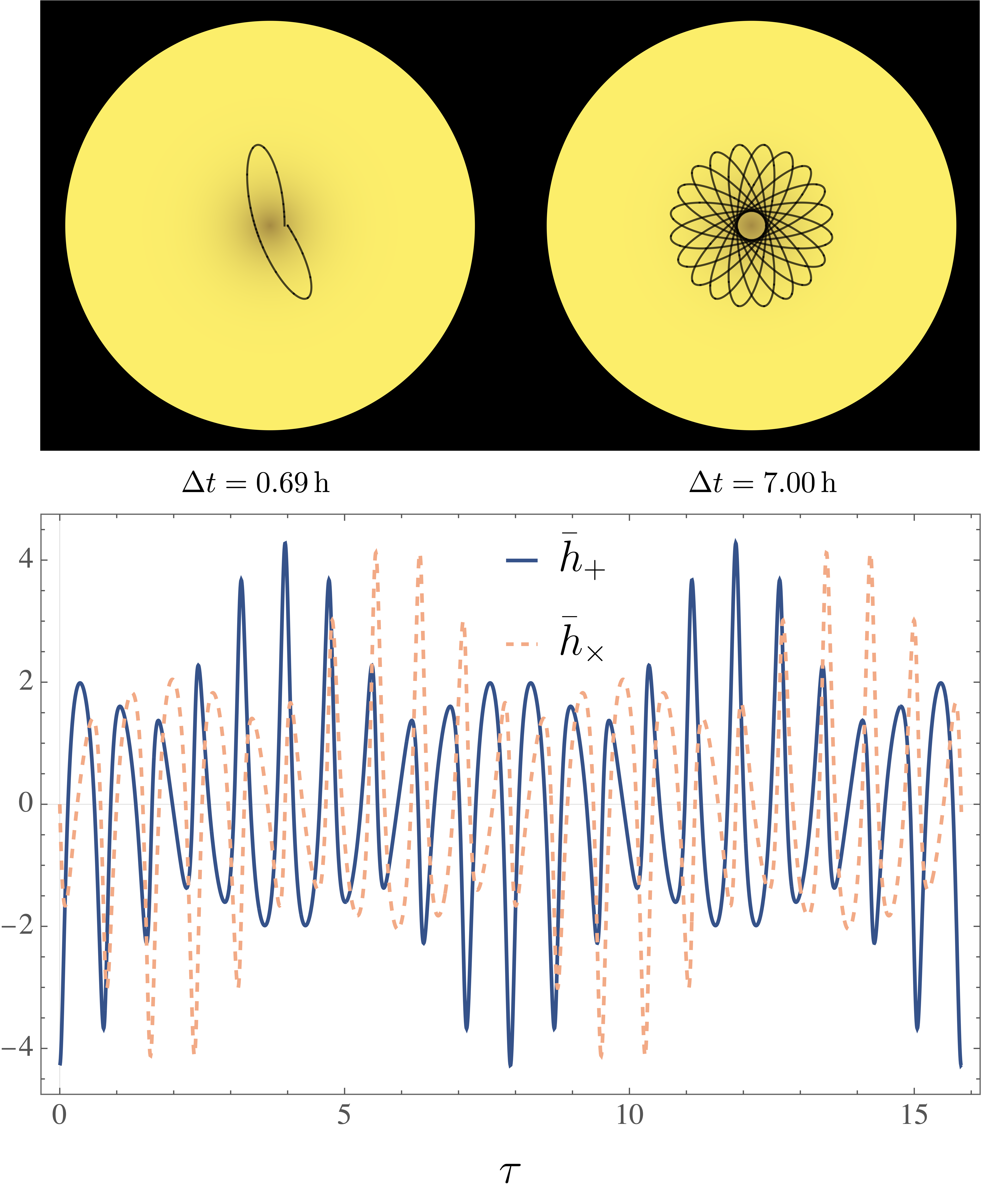
Figure 5: The top panels show the orbit of a PBH of total energy given by $\bar{E}_{\textsc{t}}=-2.3435$ and with an angular momentum such that $\bar{\ell}=0.141$. The top-left panel illustrates the path of the PBH in a complete revolution $\Delta\varphi=2\pi$, while the top-right panel shows a complete closed orbit. The corresponding GW scaled strains $\bar{h}_{+}$ and $\bar{h}_{\times}$ emitted by the system when performing the closed orbit are shown in the bottom panel, as a function of dimensionless time $\tau$.

The GW signals are depicted in the bottom panels of these figures. For instance, in Fig. 5, the top-left panel illustrates the path of a PBH covering a full $2\pi$ angular span, which takes approximately $0.69\,\text{h}$ to complete. The top-right panel shows the entire closed orbit, and the corresponding map of the emitted GW is shown in the bottom. Note that the interval of time for a closed orbit is about $7\,\text{h}$. As it is periodic, the complete signal repeats every $7\,\text{h}$, leading to a frequency of $3.97\times 10^{-5}\,\text{Hz}$. However, the interval between two successive maxima of amplitude is about $0.35\,\text{h}$, which leads to a frequency of about $8.05\times 10^{-4}\,\text{Hz}$. The same reasoning applies to Figs. 6 and 7, where the amplitude of the signal becomes larger as the eccentricity of the orbit increases.

Figure 6: The top panel shows the orbit of a PBH of total energy given by $\bar{E}_{\textsc{t}}=-1.56456$ and with an angular momentum such that $\bar{\ell}=0.141$. The corresponding GW scaled strains $\bar{h}_{+}$ and $\bar{h}_{\times}$ emitted by the system during a complete closed orbit are shown in the bottom panel.

In particular, Fig. 7 illustrates a closed semi-interior orbit with an initial condition of $r(0)=2R$, corresponding to the maximum distance the PBH reaches along its path. As can be seen, the strain signals are more intense and sharper than in the other less eccentric orbits. In this specific case, the amplitude of the strains almost achieves the maximum value predicted in Fig. 3.

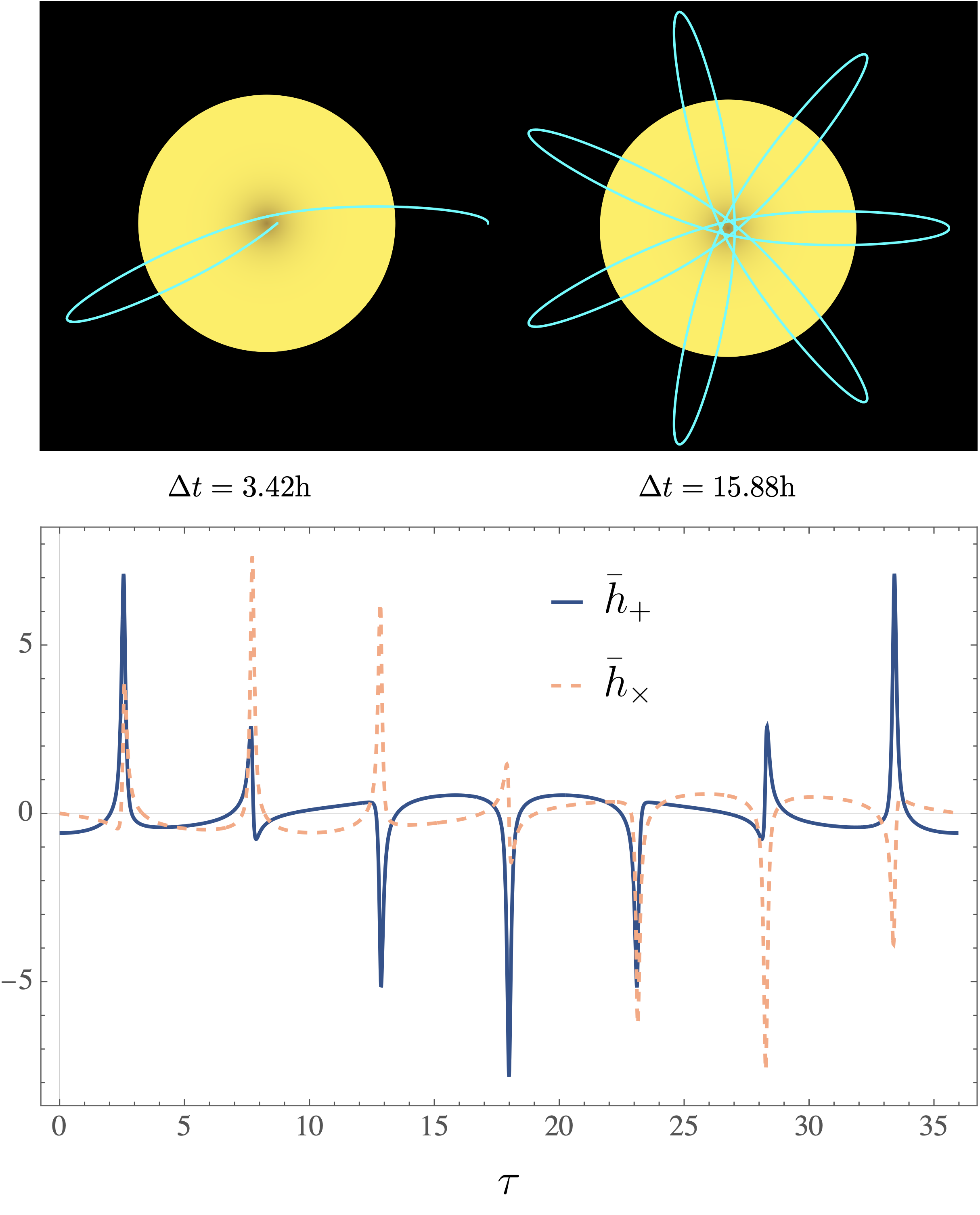
Figure 7: The top panel shows a closed semi-interior orbit of a PBH of total energy given by $\bar{E}_{\textsc{t}}=-0.57707$ and with an angular momentum such that $\bar{\ell}=0.141$. The bottom panel shows the corresponding GW scaled strains $\bar{h}_{+}$ and $\bar{h}_{\times}$ emitted by the system when performing one closed orbit, as a function of dimensionless time $\tau$.

It can be inferred from the above figures that the strain signals become sharper and more pronounced as the eccentricity of the orbits increases. This fact suggests that an orbit with null angular momentum (a free falling radial orbit) would maximize the amplitude of the strains. Suppose a PBH falls radially toward the star, starting at rest at $s_{0}$. At this point, its total energy is given by $\bar{E}_{\textsc{t}}=\bar{V}(s_{0})$, where Eq. (5) takes the form

$$\bar{V}(s)=\begin{cases}-\displaystyle\int_{s}^{1}\frac{\bar{M}(u)}{u^{2}}\text{d}u-1,&\text{if }s<1,\\ &\\ -1/s,&\text{if }s>1.\end{cases}$$ (25)

As the PBH passes through the center of the star, energy conservation requires that $\frac{1}{2}s^{\prime}(\tau)^{2}+\bar{V}(0)=\bar{V}(s_{0})$. However, $s_{0}>1$ for a semi-interior orbit, and therefore as the PBH passes through the center, its velocity is such that $s^{\prime 2}=2\left[-1/s_{0}-\bar{V}(0)\right]$. Furthermore, the scaled strain $\bar{h}_{+}$ associated with this type of orbit has the form $\bar{h}_{+}=s^{\prime 2}-\bar{M}(s)/s$, which reaches a maximum amplitude when $s=0$. In this case,

$$\bar{h}_{+}=s^{\prime 2}=-2\left[\frac{1}{s_{0}}+\bar{V}(0)\right],$$ (26)

which achieves its largest value when $s_{0}\to\infty$, such that

$$\lim_{s_{0}\to\infty}\bar{h}_{+}=-2\bar{V}(0)=2\left[1+\displaystyle\int_{0}^{1}\frac{\bar{M}(u)}{u^{2}}\text{d}u\right].$$ (27)

Additionally, note that this value depends on the full mass distribution. For the particular mass-density distribution defined by Eq. (22), we get $\bar{V}(0)=-9/2$ and hence the maximum value achieved by this strain is such that $\bar{h}_{+}=9-2/s_{0}$. If we choose $s_{0}=1.7$, as in Fig. 7, the maximum strain is $\max(h_{+})\approx 7.8$, which is close to the limit of the plot in Fig. 3 as $\bar{\ell}\rightarrow 0$. Note that the maximum possible amplitude is $9$, which corresponds to a radially free-fall trajectory starting from infinity. We emphasize that this maximum value depends on the star’s mass distribution.

In order to have an estimate of the effect that would be measured in a GW detector, suppose a PBH of mass $m$ is orbiting the Sun, as described in any of the solutions depicted in the above figures. The maximum amplitude $h^{\textsc{tt}}$ of the gravitational wave emitted by this system that would be received on Earth would be:

$$\begin{split}h^{\textsc{tt}}\approx&\;2.11\times 10^{-24}a\left(\frac{m}{10^{20}\,\text{kg}}\right)\left(\frac{M_{\odot}}{1.99\times 10^{30}\,\text{kg}}\right)\\ &\times\left(\frac{1.50\times 10^{11}\,\text{m}}{d}\right)\left(\frac{6.96\times 10^{8}\,\text{m}}{R}\right),\end{split}$$

where $a$ denotes the amplitude of the GW signal, given by the scaled strains $\bar{h}_{+}$ or $\bar{h}_{\times}$ introduced in Eqs. (13) and (14). For example, for a PBH with mass $m=10^{20}\,\text{kg}$ orbiting the Sun, the maximum amplitude of the signal received on Earth would be $h^{\textsc{tt}}\approx 10^{-23}$. We may compare such signals with those predicted from a more strongly relativistic system. Ref. Baumgarte and Shapiro (2024a) considers the GW spectrum from a bound PBH undergoing an interior orbit within a neutron star (NS), with $m=1.4\times 10^{-6}\,M_{\odot}\simeq 2.8\times 10^{24}\,\text{kg}$ and $M=1.4\,M_{\odot}=2.8\times 10^{30}\,\text{kg}$ at a distance $d=10\,{\rm kpc}$ from Earth. They find typical GW strains $h^{\textsc{tt}}\sim{\cal O}(10^{-24})$ Baumgarte and Shapiro (2024a). We may extrapolate our own results to a system involving the same PBH mass orbiting within our own Sun, which yields $h^{\textsc{tt}}\approx 3\times 10^{-20}a\sim{\cal O}(10^{-19})$. This is significantly stronger than the signal at Earth expected from a typical NS-PBH system.

V Detecting GW Signals from Individual Systems

In this section we consider the possibility of detecting GW signals from a single PBH of mass $m$ orbiting a Sun-like star, whose mass and radius we take to be $M_{\odot}$ and $R_{\odot}$, respectively. As we will see, if the PBH-star system is relatively close to the Earth—that is, if it is bound within the Milky Way galaxy rather than undergoing Hubble flow—then the typical GW signals would achieve maximum amplitude for observed frequencies at a near-Earth detector of order $f\sim{\cal O}(10^{-3}\,\text{Hz})$. Such signals would be interesting candidates for detection by the LISA gravitational-wave observatory Maggiore (2007); Seoane et al. (2023); Robson et al. (2019); Smith and Caldwell (2019). (Given the typical frequencies expected from such PBH-star systems and the peak sensitivities expected for other upcoming GW detectors, such as the Einstein Telescope and Cosmic Explorer—each of which will be optimized for GW signals with $f\sim{\cal O}(10^{0}-10^{3}\,{\rm Hz})$ Reitze et al. (2019); Abac et al. (2025)—we do not expect the GW sources considered here to be candidates for detection with those other experiments.)

To begin, we consider a source that produces time-series waveforms $h_{+}(\tau)$ and $h_{\times}(\tau)$, akin to those calculated from Eq. (12) and shown for various initial conditions in Figs. 5, 6, and 7. After converting from dimensionless time $\tau$ to source-frame time $t$ (in seconds), we sample the time-series data at a frequency of 2 Hz, as appropriate for LISA sensitivity up to $\sim 1$ Hz. We then implement the algorithm of Ref. Cooley and Tukey (1965) to compute the discrete Fourier transforms of the sampled time-series data to yield $\tilde{h}_{+}(f)$ and $\tilde{h}_{\times}(f)$.

Because the waveforms $h_{+,\times}(\tau)$ are dominated by the quadrupole moment, we may express the frequency-domain strains as Robson et al. (2019); Smith and Caldwell (2019); Maggiore (2007)

$$\begin{split}\tilde{h}_{+}(f)&=A(f)\left(\frac{1+\cos^{2}\eta}{2}\right)e^{i\Psi(f)},\\ \tilde{h}_{\times}(f)&=iA(f)\,\cos\eta\,e^{i\Psi(f)},\end{split}$$ (28)

where $A(f)$ is the amplitude, $\Psi(f)$ is the phase, and $\eta$ is the inclination of the plane of the PBH orbit with respect to the observer. Given the amplitude $A(f)$, we may construct the signal power spectral density averaged over sky locations, GW polarizations, and inclination angles $\eta$ Robson et al. (2019),

$$S_{h}(f)=\frac{A^{2}(f)}{2T_{\text{sam}}},$$ (29)

where $T_{\text{sam}}$ is the sampling interval, which we take to be the period of one complete PBH orbit. For long-lived, continuous-wave GW signals like the ones we consider here, an instrument like LISA can boost signal-to-noise compared to the instantaneous strain by using template-matching signal extraction. Taking this into account, we may calculate the angle-averaged square of the optimal signal-to-noise ratio Robson et al. (2019),

$$\langle\rho^{2}\rangle=\frac{16}{5}\int_{0}^{\infty}\frac{2fT_{\text{obs}}S_{h}(f)}{S_{n}(f)}\frac{\text{d}f}{f},$$ (30)

where $S_{n}(f)$ is the power spectral density of noise in the LISA detector averaged over angle and waveform polarization, and $T_{\text{obs}}$ is the duration of observation. The factor $(2fT_{\text{obs}})$ in the numerator arises from improved signal discrimination via template-matching. For the LISA detector, we use the parameterization of $S_{n}(f)$ in Ref. Robson et al. (2019).

The signal-to-noise ratio $\rho$ is computed by integrating over all frequencies. To compare the effective signal-to-noise at a given frequency $f$, we may define the quantity Robson et al. (2019)

$$h_{\text{eff}}^{2}(f)\equiv\frac{16}{5}f\left(2fT_{\text{obs}}\right)S_{h}(f).$$ (31)

In Fig. 8, we plot $h_{\text{eff}}(f)$ and the amplitude spectral density $\sqrt{S_{n}(f)}$ for LISA for the GW waveforms shown in Figs. 5, 6, and 7. In each case, we have set $m=2\times 10^{21}\,\text{kg}=10^{-9}\,M_{\odot}$ and $d=1.5\times 10^{8}\,\text{km}=1\,\text{AU}$. For these parameters, we see that the typical $h_{\text{eff}}/\sqrt{f}\sim\sqrt{S_{n}}$ across the LISA sensitivity range. Over the full LISA mission, with $T_{\text{obs}}=4\,\text{yr}$, we find $\rho\gtrsim{\cal O}(1)$ for several configurations. Given the form of Eq. (12), the amplitude $A(f)$, and therefore the signal-to-noise ratio $\rho$, scales linearly with $m$ and $M$ and inversely with $R$ and $d$.

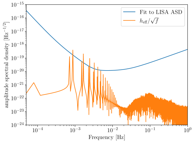
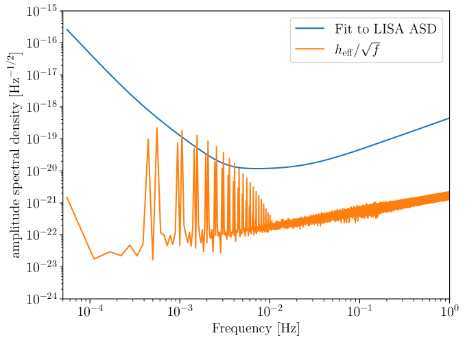
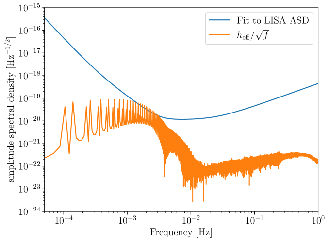
Figure 8: LISA amplitude spectral density (ASD, in blue) compared to $h_{\text{eff}}$ (orange) for various PBH-star orbital configurations. In each case we use $M_{\star}=M_{\odot}$ and $R=R_{\odot}$ for the host star, $m=10^{-9}\,M_{\odot}$ for the PBH mass, and set $d=1\,\text{AU}$. The amplitude for the signal $h_{\text{eff}}(f)$ scales as in Eq. (IV) for other selections of orbital parameters. (Top) The initial conditions as in Fig. 5, which yields $\rho=1.1$ over the 4-year LISA mission lifetime. (Middle) The initial conditions as in Fig. 6, which yields $\rho=1.0$ over the 4-year LISA mission lifetime. (Bottom) The initial conditions as in Fig. 7, which yields $\rho=0.6$ over the 4-year LISA mission lifetime. In each plot, we have averaged over sky location, GW polarizations, and orientation of the PBH orbit with respect to the detector.

As expected, each of the GW waveforms shown in Fig. 8 peaks at a frequency $f\simeq 1/t_{\text{orbit}}$. For the cases shown there, with $v_{0}\sim 10^{2}\,\text{km}\,\text{s}^{-1}$ and semi-major axis of the PBH orbit ${\cal R}_{\text{pbh}}\simeq R_{0}$, we find $f_{\text{peak}}\simeq 10^{-3}\,\text{Hz}$. In fact, upon plotting the waveforms $\tilde{h}_{+,\times}(f)$ rather than the weighted combination $h_{\text{eff}}(f)$, we find $A_{\text{peak}}\equiv A(f_{\text{peak}})\sim 10^{2}A(f_{\text{next}})$, where $A(f_{\text{next}})$ is the amplitude of the next-leading Fourier component.

For the curves shown in Fig. 8, we have averaged over sky locations when evaluating $\rho$. The results reveal an interesting trade-off: although a larger initial orbital distance enhances the amplitude of the emitted GW signal, it simultaneously leads to a lower signal-to-noise ratio, reducing the detectability of the event. In contrast, more confined orbits produce GW signals with a lower amplitude that can be detected more easily, since $\rho\geq 1$. As discussed in Refs. Robson et al. (2019); Smith and Caldwell (2019), if one knows the location of a given source, then the optimal value of $\rho$ can be improved by not performing an average over the full sky. In the present case, we remain agnostic as to where a given source might appear and hence we perform the typical all-sky averaging.

For $m=10^{-9}\,M_{\odot}$ and $M=M_{\odot}$, the orbits as simulated here should remain unaffected by dynamical friction up to a time-scale $t_{\text{dyn}}\sim 10^{-1}(M_{\odot}/m)\,t_{\text{orbit}}\sim 10^{5}\,\text{yr}$. On the other hand, if a signal detectable by LISA were to come from a small-mass PBH orbiting a Sun-like star other than our own Sun — and hence at a larger distance from the Earth than $d=1\,\text{AU}$ — then the PBH mass $m$ would need to be correspondingly larger than $10^{-9}\,M_{\odot}$. As a concrete example, for a PBH in orbit around the star Proxima Centuri, at a distance $d=4.0\times 10^{13}\,\text{km}=2.7\times 10^{5}\,\text{AU}$ from the Earth, the PBH mass $m$ would need to be $m=2.7\times 10^{-4}\,M_{\odot}$ in order to yield $\rho>1$ for a LISA detection. With that mass, $t_{\text{dyn}}\sim 1\,\text{yr}$, making the likelihood for such a detection with the LISA detector quite small.

Lastly, we note that for the plots in Fig. 8, we have used the simple quadrupole approximation when evaluating the waveforms $h_{+,\times}$, which should be sufficiently accurate for GWs in the far-field region arising from the systems we consider here. Yet if a PBH were orbiting our own Sun, the typical wavelength of the GWs, $\lambda\sim c/f_{\rm peak}$, would be comparable to the distance between the Sun and the LISA detectors, $d\sim 1\,{\rm AU}$. We leave to future work the interesting question of how near-field radiation effects might alter the predicted signals shown in Fig. 8.

VI Contribution to the Stochastic GW Background

If a significant fraction of the dark matter consists of small-mass PBHs, then such objects must have been ubiquitous throughout cosmic history. Likewise, Sun-like stars have been common throughout the universe since around redshift $z=3$, that is, over the past 11.5 Gyr Dunlop (2011). If the capture rate for small-mass PBHs by Sun-like stars is not negligible, then a significant population of bound PBH-star systems should have formed throughout the universe over time. The gravitational-wave emissions from a population of such independent sources would contribute to the stochastic GW background (SGWB). In this section we consider what contribution we might expect from PBH-star orbits to the SGWB, and whether such a contribution might be detectable via pulsar timing arrays Agazie et al. (2023); Antoniadis et al. (2023); Reardon et al. (2023); Xu et al. (2023).

We follow Ref. Lehmann et al. (2022) to estimate the PBH capture rate. (See also Refs. Khriplovich and Shepelyansky (2009); Capela et al. (2013a, b); Lehmann et al. (2021); Génolini et al. (2020); Caplan et al. (2024); Caiozzo et al. (2024); Santarelli et al. (2024); Bhalla et al. (2025).) Ref. Lehmann et al. (2022) considers several mechanisms that would yield a bound PBH orbiting a star, including energy loss by the PBH due to GW emission, dissipative dynamics such as gas drag and dynamical friction, and three-body capture and ejection, involving exchange of energy between the PBH, its host star, and a Jupiter-like planet. As noted above, for PBHs in the mass range of interest here, energy loss via GW emission remains weak, and dissipative dynamics are most effective in denser media such as gas clouds undergoing early star formation, whereas three-body capture can occur at any time over cosmic history. For the three-body scenario, Ref. Lehmann et al. (2022) estimates an equilibrium number of bound PBHs per star of the form

$$\begin{split}N_{\text{eq}}&\simeq\left(\frac{0.65+\log_{10}[M_{\star}/M_{\text{planet}}]}{3.7}\right)\left(\frac{M_{\star}}{M_{\odot}}\frac{{\cal R}_{\text{planet}}}{5\,\text{AU}}\right)^{3/2}\\ &\quad\times\left(\frac{v_{0}}{220\,\text{km}\,\text{s}^{-1}}\right)^{-3}\left(\frac{\rho_{\text{DM}}}{0.4\,\text{GeV}\,\text{cm}^{-3}}\cdot\frac{10^{14}\,\text{kg}}{m}\right),\end{split}$$ (32)

where ${\cal R}_{\text{planet}}$ is the semi-major axis of the planet’s orbit around its host star, $v_{0}$ is the typical PBH velocity in the vicinity of the stellar system (prior to capture), and $\rho_{\text{DM}}$ is the local dark matter energy density. The fiducial values are selected for the Sun-Jupiter system while also assuming that PBHs constitute all or most of the dark matter. For PBHs within the asteroid-mass range, one may therefore expect $N_{\text{eq}}\sim{\cal O}(1)$ across stellar systems, if (for example) ${\cal R}_{\text{planet}}>5\,\text{AU}$ for a given Jupiter-like planet compensates for PBHs with masses $m>10^{14}\,\text{kg}$.

Given the form of the equilibrium capture number $N_{\text{eq}}$ in Eq. (32), associated with PBH capture via three-body interactions with a host star and a Jupiter-like planet with ${\cal R}_{\text{planet}}$, we may consider PBH orbits with longer semi-major axes than the radius $R_{\odot}$ of its host star, such as ${\cal R}_{\text{pbh}}\sim{\cal O}(1\,\text{AU})\simeq{\cal O}(10^{8}\,\text{km})$. The corresponding escape velocity at such distances is $v_{\text{esc}}=\sqrt{2GM_{\star}/{\cal R}_{\text{pbh}}}\simeq 40\,\text{km}\,\text{s}^{-1}$. For such PBH orbits, the GW waveforms are strongly peaked at frequency $f_{\text{peak}}\simeq 1/t_{\text{orbit}}\simeq v_{0}/{\cal R}_{\text{pbh}}\sim 10^{-7}\,\text{Hz}$. If we approximate $A(f)\simeq A_{\text{peak}}\,\delta(f-f_{\text{peak}})$, where $A_{\text{peak}}\equiv A(f_{\text{peak}})$, then

$$\langle|\tilde{h}_{+}(f)|^{2}+|\tilde{h}_{\times}(f)|^{2}\rangle\simeq A_{\text{peak}}^{2}\,\delta(f-f_{\text{peak}}),$$ (33)

upon averaging over inclination angles $\eta$. At some cosmological distance from a near-Earth detector, given by redshift $z$, the measured frequency in the detector $f$ would be redshifted compared to the frequency $f_{r}$ that an observer at rest near the source would measure as $f=f_{r}/(1+z)$. Given that current pulsar timing arrays are sensitive to measured frequencies in the range $10^{-9}\,\text{Hz}\leq f\leq 10^{-7}\,\text{Hz}$ Agazie et al. (2023); Antoniadis et al. (2023); Reardon et al. (2023); Xu et al. (2023), we therefore consider the contributions from a cosmic collection of such PBH-star systems, with ${\cal R}_{\text{pbh}}\sim{\cal O}(1\,\text{AU})$.

For the peak amplitude $A_{\text{peak}}$, we again fix the star mass $M_{\star}=M_{\odot}$ and $R=R_{\odot}$ and consider a typical comoving distance of the PBH-stellar system to Earth to be $d=3\times 10^{13}\,\text{km}=1\,\text{pc}$. Taking the dimensionless amplitude $a\sim{\cal O}(10)$, as in Figs. 5–7, then from Eq. (IV) we may estimate

$$A_{\text{peak}}(z)\approx 10^{-30}\left(\frac{m}{10^{20}\,\text{kg}}\right)\left(\frac{1\,\text{AU}}{{\cal R}_{\text{pbh}}}\right)\left(\frac{1\,\text{pc}}{d_{\text{com}}}\right)\frac{1}{1+z},$$ (34)

where the factor $1/(1+z)$ takes into account that the amplitude near Earth from a source at comoving distance $d_{\text{com}}$ will be redshifted by cosmic expansion.

A collection of independent PBH-star systems would contribute incoherently to the SGWB intensity, with

$$|A_{\text{pbh}}^{\text{total}}|^{2}=\sum_{i}|A_{i}|^{2}\simeq\int N(z)\,|A_{\text{peak}}(z)|^{2}\text{d}z,$$ (35)

where $N(z)$ counts the number of such sources as a function of redshift. To estimate $N(z)$, we write

$$N(z)\,\text{d}z\simeq N_{\text{eq}}\,f_{\odot}\,N_{\odot}\,n_{\text{gal}}\,\text{d}V(z),$$ (36)

where the capture rate $N_{\text{eq}}$ is given in Eq. (32), $f_{\odot}\simeq 0.2$ is the fraction of Sun-like stars within the Milky Way galaxy, $N_{\odot}\simeq 10^{11}$ is the total number of stars in the Milky Way galaxy, and $n_{\text{gal}}\simeq 2\,\text{Mpc}^{-3}$ is the number density of galaxies comparable to the Milky Way within our local neighborhood (considering the Milky Way and Andromeda to be the baseline). The volume factor out to redshift $z$ may be written in terms of the comoving volume element Hogg (1999)

$$\text{d}V_{c}=R_{\textsc{h}}\frac{d_{M}^{2}(z)}{E(z)}\text{d}\Omega\,\text{d}z,$$ (37)

where $R_{\textsc{h}}\equiv cH_{0}^{-1}=4350\,\text{Mpc}$ is the present value of the Hubble radius, $\text{d}\Omega$ is the solid angle element, $d_{M}(z)$ is the comoving transverse distance,

$$d_{M}(z)=R_{\textsc{h}}\int_{0}^{z}\frac{\text{d}z^{\prime}}{E(z^{\prime})},$$ (38)

and $E(z)$ is the dimensionless Hubble parameter, defined via $H(z)=H_{0}E(z)$, with

$$E(z)\equiv\left[\Omega_{r}(1+z)^{4}+\Omega_{m}(1+z)^{3}+\Omega_{k}(1+z)^{2}+\Omega_{\Lambda}\right]^{1/2}.$$ (39)

The physical three-volume of a sphere centered on the Earth out to redshift $z$ is related to $\text{d}V_{c}$ as $\text{Vol}(z)=(1+z)^{3}\int\text{d}V_{c}$. Combining these factors, using Eq. (32) for $N_{\text{eq}}$ and the best-fit $\Lambda$CDM values for each $\Omega_{i}$ Aghanim et al. (2020) yields

$$\begin{split}A_{\text{pbh}}^{\text{total}}&\approx 10^{-21}\left(\frac{m}{10^{20}\,\text{kg}}\right)^{1/2}\left(\frac{{\cal R}_{\text{planet}}}{5\,\text{AU}}\right)^{3/4}\\ &\quad\quad\times\left(\frac{1\,\text{AU}}{{\cal R}_{\text{pbh}}}\right)\left(\frac{1\,\text{pc}}{d_{\text{com}}}\right),\end{split}$$ (40)

upon integrating out to $z=3$ to include the dominant epoch of Sun-like star formation Dunlop (2011). For simplicity, we have retained the typical dark-matter characteristics as in Eq. (32), as well as keeping $M_{\star}=M_{\odot}$ and $M_{\text{planet}}=M_{\text{Jupiter}}$.

This amplitude may be compared with the SGWB amplitude reported by the NANOGrav collaboration, $A_{\text{SGWB}}\simeq 8\pm 1\times 10^{-15}$. (See Fig. 1 in Ref. Afzal et al. (2023).) The expected contribution to the SGWB from a collection of PBH-star systems would be comparable to the reported $A_{\text{SGWB}}$ if, for example, the typical PBH mass were $m\sim 10^{26}\,\text{kg}$, the typical planetary semi-major axis ${\cal R}_{\text{planet}}\sim 10^{2}\,\text{AU}$, and the typical comoving distance $d_{\text{com}}\sim 10^{-2}\,\text{pc}$. Although a typical PBH mass $m\simeq 10^{26}\,\text{kg}$ is considerably larger than the asteroid-mass range within which PBHs could constitute all of dark matter, present observational bounds (such as microlensing) are consistent with $f_{\text{pbh}}\simeq 0.1$ for $m\simeq 10^{26}\,\text{kg}$ Carr and Kühnel (2020); Green and Kavanagh (2021); Carr et al. (2024); Escrivà et al. (2022); Gorton and Green (2024). Moreover, $t_{\text{dyn}}\sim 10^{-1}(M_{\odot}/m)\,t_{\text{orbit}}\sim 10^{3}\,\text{yr}$, suggesting that the orbits of PBHs with these masses would be stable against dynamical friction parametrically longer than the time-scales $\Delta T\sim 1/f_{\text{min}}\sim 10^{2}\,\text{yr}$ to which present-day pulsar timing arrays are sensitive.

In addition to considering the amplitude of the contribution to the SGWB, we may also consider the spectral index $\gamma$ associated with such a collection of incoherent sources. The typical source that is expected to contribute to the SGWB with frequencies to which pulsar timing arrays are sensitive is binary inspirals of supermassive black holes (SMBHs). These yield a spectral index $\gamma=13/3$, which is in tension with the value of $\gamma$ inferred by the NANOGrav collaboration from their analysis of their 15-year dataset Afzal et al. (2023); Sato-Polito et al. (2025). To estimate the spectral index $\gamma$ that would arise from an incoherent collection of small-mass PBHs orbiting Sun-like stars, we follow Ref. Phinney (2001) and parameterize the energy density in GWs as

$$\Omega_{\text{gw}}(f)=\frac{1}{\rho_{c}}\frac{\text{d}\rho_{\text{gw}}(f)}{\text{d}\ln f}=\frac{8\pi^{4}}{H_{0}^{2}}f^{5}\frac{\Phi(f)}{\Delta f},$$ (41)

where $\rho_{c}$ is the critical density for a spatially flat universe and $\Delta f=1/T_{\text{obs}}$ is related to the observing window. The function $\Phi(f)$ is typically parameterized as a power law Afzal et al. (2023),

$$\Phi(f)=\frac{A^{2}}{12\pi^{2}}\Delta f\left(\frac{f}{\text{yr}^{-1}}\right)^{-\gamma}\,\text{yr}^{3},$$ (42)

in terms of a GW waveform amplitude $A$. The energy density $\Omega_{\text{gw}}(f)$ therefore scales as $\Omega_{\text{gw}}(f)\sim f^{5-\gamma}$ with some spectral index $\gamma$.

The energy density may be computed as Phinney (2001)

$$\Omega_{\text{gw}}(f)=\frac{1}{\rho_{c}c^{2}}\int\text{d}z\,N(z)\frac{1}{1+z}\left(f_{r}\frac{\text{d}E_{\text{gw}}}{\text{d}f_{r}}\right)\bigg{|}_{f_{r}=f(1+z)},$$ (43)

with

$$\frac{\text{d}E_{\text{gw}}}{\text{d}f_{r}}=\frac{2\pi^{2}c^{3}}{G}\,d_{M}^{2}(z)f^{2}\langle|\tilde{h}_{+}(f)|^{2}+|\tilde{h}_{\times}(f)|^{2}\rangle.$$ (44)

Making use of Eq. (33) for a collection of independent PBH-star systems then yields

$$\begin{split}\left(f_{r}\frac{\text{d}E_{\text{gw}}}{\text{d}f_{r}}\right)\bigg{|}_{f_{r}=f(1+z)}&\simeq\frac{2\pi^{2}c^{3}}{G}d_{M}^{2}(z)f^{3}(1+z)^{3}\\ &\quad\times A_{\text{peak}}^{2}(z)\,\delta\left[f(1+z)-f_{\text{peak}}\right].\end{split}$$ (45)

Substituting into Eq. (41) suggests that

$$\gamma\simeq 2$$ (46)

for such a collection of sources.

If the SGWB consisted of a combination of types of sources, such as SMBH binary inspirals (with $\gamma=13/3$) as well as bound PBH-star orbits (with $\gamma\simeq 2$), then the weighted average $\gamma_{\text{avg}}$ would fall closer to the central value $\gamma\simeq 3.4\pm 0.2$ inferred by the NANOGrav collaboration (see Fig. 1 of Ref. Afzal et al. (2023)), if the corresponding amplitudes $A_{\text{SMBH}}$ and $A_{\text{pbh}}^{\text{total}}$ for each type of source were themselves comparable.

VII Final Remarks

In this work, we investigated the GW emission produced by a primordial black hole orbiting a Sun-like star, whose mass distribution is illustrated in Fig. 2. The equation governing the GW production was written in such a way that all the physical parameters characterizing the system appear as a coefficient of the dynamical term, given by the second derivative of the quadrupole moment of the system. Consequently, our findings can easily be applied to systems in which the central star has a mass distribution with a similar profile. The only need is to adjust the physical parameters to match the values associated to the new system.

The shape of the orbits will naturally depend upon the initial conditions, but the magnitude of the effect will mostly be given by the coefficient appearing in the strain tensor in Eq. (12). For instance, an interesting system to investigate is one involving a red dwarf (spectral type M), which is reported to be the most populous type of star in the galaxy. Red dwarfs are generally less massive than the Sun, with typical masses ranging from 0.08 to 0.6 $M_{\odot}$. Their radii are smaller, too, typically spanning from 0.1 to 0.6 $R_{\odot}$. Regarding their mass-density distribution, they are claimed to be denser near the center, as compared to the Sun. For a dwarf of radius $0.1\,R_{\odot}$ and mass $0.1\,M_{\odot}$, the central mass-density is expected to be about $\rho_{C}\approx 500\,\text{g}\,\text{cm}^{-3}$ Chabrier and Baraffe (1997). Although a steeper mass-density gradient is expected in these stars, its influence on the magnitude of the GW amplitude does not significantly enhance the effect, as the ratio $M_{\star}/R$ is approximately the same as that of the Sun, $M_{\odot}/R_{\odot}$. However, given that their distance to the Earth is much larger than that of our Sun, their GW strains will be several orders of magnitude smaller. For instance, the closest red dwarf we know is Proxima Centauri, approximately $4.02\times 10^{13}\,\text{km}=1.30\,{\rm pc}$ away. The amplitude of a GW produced by a PBH of mass $10^{20}\text{kg}$ orbiting such dwarf star, and measured near Earth, would be $h^{\textsc{tt}}\approx 10^{-28}$.

It is interesting to note that if a constant density profile is assumed, the corresponding gravitational potential experienced by the orbiting particle becomes harmonic ($\sim r^{2}$) when the particle is in the interior of the star and Keplerian ($\sim r^{-1}$) when it is in the exterior region. Thus, according to Bertrand’s theorem Goldstein et al. (2002), all bounded solutions will result in closed orbits if the particle’s path is entirely inside the star or entirely outside it. However, for hybrid orbits, the trajectories will be generally open but could be closed for specific initial conditions De Lorenci et al. (2024).

In this work, we examined the particular case in which the observer is placed orthogonally to the plane of the PBH’s orbit. The generalization to an arbitrary observer location is straightforward, and it can be shown that it results in slightly different strains, though they remain of the same order of magnitude. In particular, for the case of a PBH that is orbiting the Sun in the same plane as the Earth does, one of the strains could identically vanish, while the other would remain unchanged. More general configurations, depending on the observer’s position relative to the orbital plane, would lead to GW strains showing different patterns, when compared to the orthogonal configuration.

Finally, we have computed expected GW strains arising from a small-mass PBH orbiting a Sun-like star and considered whether such systems could yield detectable GW signals. Whereas it is unlikely that such an isolated system would yield a large enough amplitude to be detected by LISA, we find regions of parameter space in which a large collection of such systems, dispersed throughout the Universe over much of cosmic history, could contribute in a measurable way to the stochastic gravitational-wave background (SGWB). Moreover, the spectral index expected for such a large collection of incoherent sources would help alleviate the present tension with the recent NANOGrav measurement, under the assumption that the signal arises predominantly from the binary inspirals of supermassive black holes.