Event Signal Filtering via Probability Flux Estimation

Abstract

Events introduce a novel paradigm for perceiving scene dynamics through asynchronous sensing, yet their inherent randomness leads to significant signal degradation. Event signal filtering emerges as a crucial process to enhance signal fidelity by mitigating internal randomness and ensuring consistent outputs across varying acquisition conditions. Unlike traditional time series describing steady-state system behaviours through predefined temporal sampling, events capture transient dynamics with dual information encoding: polarity values and event intervals, so the modelling of event signal is much more complex and difficult. To address this challenge, the theoretical foundation of event generation model is revisited in the framework of the diffusion processes. It is perceived that the distribution of state and process information within events can be modelled by the continuous probability flux at threshold boundaries of the underlying irradiance diffusion process. With this knowledge, a generative online event signal filtering framework named Event Density Flow Filter (EDFilter) is proposed in this paper. The idea behind it is to model the event correlation by estimating continuous probability flux from a series of discrete input events with nonparametric kernel smoothing, then obtain the filtered events by resampling from the estimated probability flux. Temporal and spatial kernels are proposed to fit observed events in a time-varying optimization manner, ensuring the best filtered probability flux at any given time. A fast recursive solver with O(1) complexity is also proposed by introducing state-space models with lookup tables (LUTs) for likelihood computation. Additionally, a real-world benchmark dataset, the Rotary Event Dataset (RED) is presented, which contains microsecond-level ground-truth scene irradiance for full-reference event signal filtering evaluation. Extensive experiments of various tasks, event signal filtering, super-resolution, and direct event-based blob tracking, validate the effectiveness and advantage of the proposed method. Significant performance improvements in some downstream applications such as SLAM and video reconstruction also demonstrate its superiority.

1 Introduction

Events introduce a new visual sensing paradigm that employs asynchronous value-triggered timestamps instead of conventional synchronous time-based frames for visual information representation. This modality is captured through specialized neuromorphic sensors (commonly called event cameras or dynamic vision sensors), which generate discrete events when the perceived scene irradiance changes reach certain thresholds [1, 2, 3]. Due to this working principle, events have very short response time and low redundancy, making them a great candidate for visual motion perception [4, 5, 6, 7].

However, perceived events are not idealized scene motion representation due to imperfections in the manufacturing process and working environment, affecting the range of possible applications. For example, structural CMOS mismatch for individual cameras causes event pixels to respond differently against the same stimulus, and electronic noise causes random fluctuation in the precise event count and timing [8, 9]. Such phenomenons are inevitable under real capturing environments, necessitating the development of effective event signal filters to ensure consistent outputs across varying acquisition conditions.

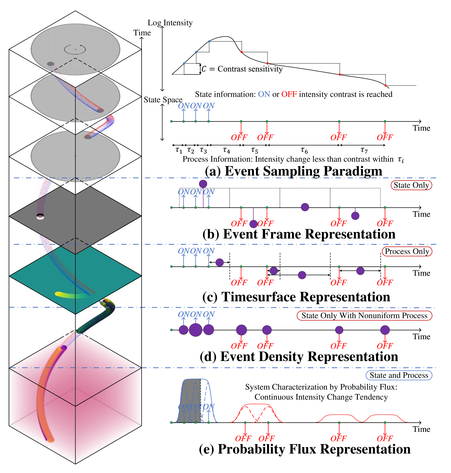
Figure 1: Overview of existing event representations. Event sampling paradigm (a) showing that an event is generated when the logarithm intensity change reaches certain thresholds. Some methods [10, 11, 12, 13] adopt the event frame representation (b), which counts the number of events within an interval to represent averaged intensity difference so no process information is kept. Some methods [14, 15, 16] adopt the timesurface representation (c) which calculates the duration since the last event happened so the state (polarity) information is discarded. There are others [17, 18, 19, 20, 21] that directly operate on the x-y-p-t event tensor (d) to derive a representation for noise event classification, which can be regarded as modifying the state information with a classification probability and viewing the sampling process as fixed. The proposed probability flux (e) characterizes system transient behavior by representing the continuous intensity change tendency, so the state and process information can be derived accordingly.

One of the most distinctive challenges in designing event signal filters is to precisely capture the transient behavior of the system reflected by the irregularly sampled event signal, as shown in Fig. 1. For a given pixel, the underlying log intensity changes as time varies, and an ON/OFF event is generated once it reaches the ON/OFF threshold, as shown in Fig. 1(a). Since the exact timestamp and polarity for the intensity crossing event can’t be determined beforehand, the transient behavior of the underlying system is collectively represented by the event polarity values and event time intervals, which correspond to the state and process information of the underlying system. In contrast, ordinary methods can only describe steady-state behaviours since all variations within the predefined sampling moments are integrated into discrete state values, which are just the average performance as shown in Fig. 1(b-d). Traditional frame-based methods can only model the correlation between discrete state values and are therefore insufficient when dealing with event signal.

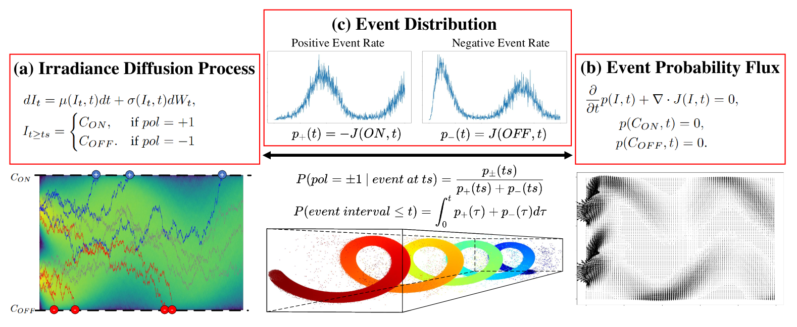
Figure 2: Physical meaning of event probability flux. The perceived logarithm scene intensity is driven by a diffusion process (a) with ON/OFF boundaries to generate events, represented by the absorbing boundary conditions. Observing that no trajectories appear or disappear out of nowhere, this process also follows continuity equation (b), where probability flux can be derived to represent event distribution (c).

To this end, we revisit the event generation model in the framework of the diffusion process to derive the required physical quantities for describing the relationship between the underlying system and event distribution. As shown in Fig. 2(a), under real environments, the perceived log intensity signal is perturbed by noise, and if the perturbation can be represented by an additive term dependent on a white noise variable in the differential form, it is called a diffusion process. Events are randomly generated once this process reaches the ON/OFF threshold, and the process is then reset to an initial distribution. To model how this process reaches the ON/OFF threshold, it’s possible to derive the probability flux from the transition probability function as shown in Fig. 2(b), which describes the intensity change tendency at any time, then the probability flux at the ON/OFF boundary is the distribution function of events generated from all possible trajectories that cross the thresholds within the time interval. With the probability flux, the distribution of state and process information can be derived accordingly as shown in Fig. 2(c), so the transient behavior and the corresponding uncertainties can be fully characterized.

However, directly solving the probability flux from the model definition is intractable in most cases. To make it a feasible solution for event signal filtering, this paper proposes to model it using nonparametric kernel smoothing and perform optimization based on the observed event signal recursively. With the best available event generative model, an online event signal filtering method is proposed accordingly, making this a generative online event signal filtering framework. It is denoted as Event Density Flow Filter or EDFilter which uses an equivalent boundary probability flux representation as event density flow for easier model construction. The proposed EDFilter consists of three components working progressively to predict, update and reconstruct the event density flow.

Specifically, a nonparametric sequential density flow model is proposed to predict the event density flow based on the observation that real events are likely to be clumped within a short period while fake events are not, modelled by a combination of continuous-time density kernels. By employing the maximum likelihood estimation recursively in the calculation, the optimal model parameters are estimated to obtain transient event occurrence probability. Further density flow updating is performed by adaptively selecting a few local basis density kernel vectors and optimize the $L_{p}$ reconstruction cost, effectively exploiting the directionality and sparsity of event density flow within a small local region. Finally, the density reconstruction part recursively merges individual density estimate into continuous density flow using application-dependent sampling point selection and zero-order hold filter, then filtered events can be sampled back with arbitrary event number and resolution. An O(1) implementation is proposed accordingly by employing state-space models and look-up tables (LUTs) for asynchronously computing the likelihood function and quick solution search.

Lastly, since most existing real-world event quality evaluation metrics depend on event labels, which are not appropriate for generative filtering methods, this paper proposed a new benchmark dataset called Rotary Event Dataset (RED) to provide ground-truth scene irradiance level based on a high-precision and high-speed motion system with a microsecond-synchronized motor encoder of 0.003° angular precision. Two event camera models are used to capture the rotary motion of 10 illusory binary texture patterns under 2 illumination and 3 speed preset conditions, resulting in a total of 60 event sequences of different motion types and speeds. Ground-truth irradiance changes can be obtained by synchronizing the camera with printed texture patterns, so that tasks including event filtering, super-resolution and direct blob tracking can be evaluated all at once. Extensive experiments on both the proposed and existing datasets demonstrate the superiority of the proposed method on the 3 tasks with only a 5$\mu$s computational delay on a single core of R9-7945HX CPU. Further applications including SLAM and scene reconstruction show that it also helps improve downstream performance.

In conclusion, the contributions of this paper are:

1. A generative online event signal filtering framework EDFilter is proposed to model event correlation by estimating continuous probability flux, which can achieve event signal filtering by generating filtered events with resampling.

2. The probability flux is estimated by predicting, updating, and reconstructing the event density flow using kernel smoothing, an algorithm designed to work asynchronously with O(1) complexity.

3. An event quality evaluation benchmark dataset RED is proposed to provide ground-truth scene irradiance level with nanosecond resolution under varying capturing conditions for a comprehensive evaluation of event signal filters.

4. Experimental results on tasks including event signal filtering, super-resolution and direct blob tracking validate the effectiveness and advantage of the proposed method, and further applications including SLAM and video reconstruction show significant performance improvements.

2 Related Work

Event Signal Filtering. Existing event signal filtering methods are mainly concerned with event denoising. Delbruck et al.[17] first proposed to pass events that are supported by recent nearby past events to output. It is the prototype of all subsequent density-based denoising methods [22, 23, 18, 14, 19], which use the number of events in fixed neighborhood to discriminate real events from noise. Liu et al.[22] reduced the memory requirement for storing density value by sub-sampling. Khodamoradi et al.[23] further reduced it to $\mathcal{O}(N)$ by introducing two memory cells assigned to each row and column. Feng et al.[18] proposed a 2-step event denoising method using event density in fixed intervals, where the discrimination threshold must be offline estimated using information from manually selected static part. Zhang et al.[19] proposed to use a sub-quadratic clustering algorithm on density values to discriminate signals. However, all these methods are unable to predict where events do not exist, and parameter selection requires human intervention. Another class of algorithms considers noise to be DVS events that do not represent an idealized motion. Mueggler et al.[24] used local plane-fitting to estimate the velocity of each event, which is used to label each event with its lifetime. Wang et al.[20] proposed to filter out events that have abnormal velocity to achieve event denoising. Wang et al.[15, 25] further incorporates Active Pixel Sensor (APS) frame information to guide the event denoising. Baldwin et al.[16] proposed an event representation based on stacked local timestamp (or timesurface) and trained a classification convolutional neural network to discriminate each event as signal or noise. Guo et al.[14] proposed a lightweight multilayer perceptron network with only 2 hidden layers and 2k weights for event denoising for high-efficiency denoising. However, all the aforementioned methods act in a discriminative way. For generative methids, Duan et al.[10, 11] adopt another event representation as stacked event frames where each pixels contains the event number information. A 3D-UNET was proposed accordingly to denoise and super-resolve the generated frames, and events are returned back by even redistribution from the generated frames. However, since exact timing information is completely ignored, it’s insufficient under highly dynamic scenes. Spatial diffusion of events also exists due to the nature of convolution operation.

Event Generation Models. There are very few attempts for direct modelling of asynchronous events. Lichtsteiner et al.[1] first proposed to regard generated events as a stochastic process by random thresholding on a continuously changing log intensity from the hardware perspective. Hu et al.[9] further extends this idea and proposed a realistic event emulator from video sequences. Gracca et al.[26] presented a tutorial on the detailed event noise model but it’s still too complicated to be applied in event signal processing. On the contrary, there are some embedded asynchronous spike models within other vision tasks. Wang et al.[27] proposed an asynchronous kalman filter for intensity reconstruction on a hybrid event-frame setup where each event triggers an update of estimated scene intensity. Liu et al.[28] proposed to formulate ego-motion pose estimation task as a state estimation problem for a finite-state hidden Markov model subject to an asynchronous event-triggering mechanism. Gu et al.[29] proposed to use spatial-temporal poisson point process for event alignment. Li et al.[21] proposed to use condition intensity function to measure the distance between two spike streams in the corresponding reproducing kernel Hilbert space (RKHS). Lin et al.[30] proposed to model events as the result of random irradiance crossing driven by a linear Stochastic Differential Equation (SDE) and derive the coefficients from video frames for event simulation. These models, however, either require additional information or are too coarse to accommodate precise event signal modelling.

Event Quality Evaluation Metrics and Datasets. Most existing event quality evaluation metrics are an adaption of discriminative metrics, often coupled with the captured or simulated datasets. Padala et al.[31] proposed to use the percentage of Signal/Noise Remaining (PSR/PNR) to evaluate the performance of event filtering, where signals are defined as all events that fall into the manually generated bounding box. Feng et al.[18] proposed to use the number of incorrectly filtered or passed events where the criterion is based on the estimated density with KDE. Baldwin et al.[16] combined the APS frame and IMU readout to generate event probability mask at around 50 frames per second and proposed the first event denoising dataset DVSNOISE20. Guo et al.[14] proposed to use the Receiver Operating Characteristic (ROC) curve for comparison over a varying discrimination threshold and proposed the DND21 dataset which contains both real and simulated sequences. All the above metrics are just variations of binary classification metrics, which are not related to scene radiance change. Duan et al.[10] proposed to use MSE training loss between projected event frames, and there is no ground-truth, which has been fixed by their further work in [11] with the Ref-E dataset by generating ground-truth events using simulation. Ding et al.[32] proposed a non-reference event denoising metric Event Structural Ratio (ESR) and a large scale multi-level benchmark dataset E-MLB for generic event quality evaluation, but it doesn’t reflect absolute scene radiance change. Currently it’s hard to compare generated events with scene radiance change due to the high temporal resolution of event cameras and the complexity of natural scenes, which impose irreducible ambiguities for deterministic event filtering analysis.

3 Approach

3.1 Event Signal Modelling Based on Probability Flux

Before introducing the details of an event signal filter, it’s important to understand what physical quantity the events reflect. This section is devoted to clarifying that probability flux is such a quantity by providing a full characterization of the state and process information of events. This is achieved by modelling events as exit times of the underlying irradiance intensity diffusion process.

From the camera working principle [17], scene irradiance is logarithmically converted into voltage levels at each pixel with composite perturbation. To describe its time-varying behavior, a diffusion process model separates it in differential form by a deterministic drift from the real scene irradiance change and a random noise related to operating temperature. Ignoring all higher-order effects, this process can be modelled by a stochastic differential equation (SDE):

$$d\bm{I}_{t}=\bm{\mu}(\bm{I}_{t},t)dt+\bm{\sigma}(\bm{I}_{t},t)d\bm{W}_{t},$$ (1)

where $\bm{I}_{t}=(I(\bm{x},t))_{\bm{x}\in[0,W)\times[0,H)}$, is the diffusion process of logarithmic scene irradiance with a spatial resolution of $W\times H$, $\bm{\mu}(\bm{I_{t}},t)$ is the real irradiance time derivative, $\bm{\sigma}(\bm{I}_{t},t)$ is the thermal noise level and $\bm{W}_{t}$ is standard multivariate wiener process with formal derivative as $\frac{d\bm{W}_{t}}{dt}=\bm{n}_{t}$, where $\bm{n}_{t}$ is a standard Gaussian white noise vector.

However, this process will stop due to the reset mechanism: once any element of $\bm{I}_{t}$ reaches the $C_{ON/OFF}$ contrast threshold, an event is generated and $\bm{I}_{t}$ is reset to an initial distribution. The first time this process reaches out the $(C_{OFF},C_{ON})$ is called an exit time [33], and is exactly the definition of an event timestamp:

$$ts:=\inf\{\tau\in T|\bm{I}_{\tau}\notin D=(C_{OFF},C_{ON})^{W\times H}\}.$$ (2)

Let $\bm{x}$ be the pixel where the boundary crossing occurs, since there are only two possible directions for the boundary crossing, event polarity is defined as the exit boundary:

$$pol:=\begin{cases}+1,&\text{if $I(\bm{x},ts)=C_{ON}$},\\ -1,&\text{if $I(\bm{x},ts)=C_{OFF}$},\end{cases}$$ (3)

or abbreviated as $\pm$.

To derive the distribution for the state and process information from this bounded SDE, the Fokker-Planck equation with absorption boundaries is introduced. Assuming this process starts at $t=0$ with initial distribution $p_{0}(\bm{I})$, then the transition probability function $p(\bm{I},t)$ satisfies:

$$\partial_{t}p(\bm{I},t)=Lp(\bm{I},t)\qquad\forall\bm{I}\in D,$$ (4)

$$L=-\partial_{i}\mu_{i}(\bm{I},t)+\partial_{i}\partial_{j}B_{ij}(\bm{I},t),$$ (5)

$$\bm{B}(\bm{I},t)=\frac{1}{2}\bm{\sigma}(\bm{I},t)\bm{\sigma}(\bm{I},t)^{T},$$ (6)

$$p(\bm{I},0)=p_{0}(\bm{I}),$$ (7)

$$p(\bm{I},t)=0\qquad\forall\bm{I}\in\partial D,$$ (8)

where the Einstein summation convention is understood and $p(\bm{I},t)$ is the probability density of logarithm irradiance. The absorbing boundary condition Eq. 8 comes from the fact that once the threshold is reached, the process never returns and stays there forever as an exited event. The boundary behavior is derived in another way by thinking of probability as a heterogeneous fluid, ant then the probability flux to the boundary is related to the transition probability function via the transport equation:

$$\partial_{t}p(\bm{I},t)+\nabla\cdot\bm{J}(\bm{I},t)=0\qquad\forall\bm{I}\in D,$$ (9)

$$J_{i}(\bm{I},t)=[\mu_{i}(\bm{I},t)-\partial_{j}B_{ij}(\bm{I},t)]p(\bm{I},t),$$ (10)

$$p_{\pm}^{k}(t)=\int_{\{\bm{I}\in\partial D\mid I_{k}=C_{ON/OFF}\}}\bm{J}(\bm{I},t)\cdot\bm{n}dS,$$ (11)

where $\bm{J}(\bm{I},t)=\{J_{i}(\bm{I},t)\}$ is the probability flux density of this diffusion process, $\bm{n}$ is the unit outer normal and $p_{\pm}^{k}(t)$ is the probability density function of the ON/OFF event at the $k$th pixel. To show that the internal and boundary behavior jointly describe all possible irradiance trajectories at any time, let $\bm{p}_{\pm}(t)=\{p_{+}^{k}(t),p_{-}^{k}(t)\}$, then the population of irradiance trajectories that don’t generate an event is:

$$\begin{split}\mathcal{N}(t):&=\int_{D}p(\bm{I},t)dV\\ &=\mathcal{N}(0)-\int_{D}\int_{0}^{t}\nabla\cdot\bm{J}(\bm{I},\tau)d\tau dV\\ &=\mathcal{N}(0)-\int_{0}^{t}\int_{\partial D}\bm{J}(\bm{I},\tau)\cdot\bm{n}dSd\tau\\ &=\mathcal{N}(0)-\int_{0}^{t}\|\bm{p}_{\pm}(\tau)\|_{1}d\tau,\end{split}$$ (12)

where the third equation can be derived by applying Gauss’s theorem using Eq. 9.

With the above definitions, it’s possible to derive the distribution of the state and process information of an event at pixel k as:

$$P(pol=\pm 1~|~\text{event at }ts)=\frac{p_{\pm}^{k}(ts)}{p_{+}^{k}(ts)+p_{-}^{k}(ts)},$$ (13)

$$P(\text{event interval }\leq t)=\int_{0}^{t}p_{+}^{k}(\tau)+p_{-}^{k}(\tau)d\tau.$$ (14)

In other words, an event signal characterizes the transient behavior of real scene dynamic change by providing observations of the probability flux at threshold boundaries, which is related to the real scene irradiance by Eqs. 1, 2, 3, 4, 5, 6, 7, 8, 9, 10, 11, 12, 13 and 14. This paper proposes to achieve event signal filtering by estimating the probability flux.

3.2 Filter Design by Estimating Event Density Flow

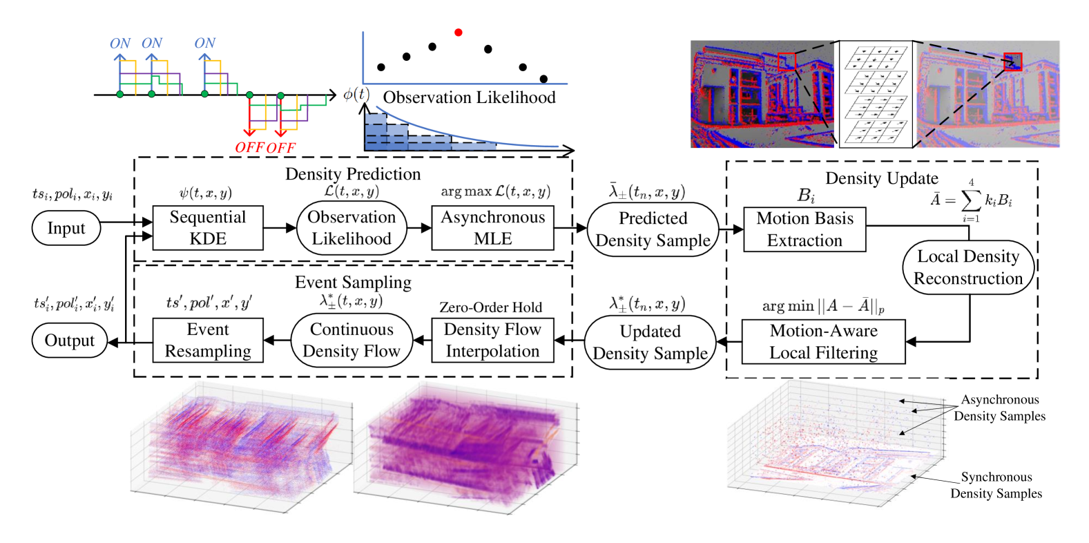
Figure 3: Workflow of the proposed EDFilter. The density prediction part generates the predicted density sample by sequentially performing KDE on input events and select the best kernel by maximizing the event observation likelihood. Then the density update part spatially merges the density samples with a motion-aware sparsity-preserving local filter to generate updated density samples. After that, the event sampling part interpolates the continuous event density flow using zero-order hold and resamples filtered events for output, which will also activate the density prediction part in an application-dependent way to alleviate the effect of abnormal integral.

Although it’s possible to construct a model for the deterministic drift $\bm{\mu}(\bm{I},t)$ and noise level $\bm{\sigma}(\bm{I},t)$ and solve the bounded Fokker-Planck Eqs. 9 and 10 for the exact expression of the state and process distribution, the complexity of these equations prevent us from deriving any feasible solution. Therefore, this paper proposes to directly model the ON/OFF probability flux using nonparametric kernel smoothing as a proxy for system modelling. To achieve this, first an equivalent formulation of the ON/OFF probability flux is derived to make the solution space less constrained, which is denoted as event density flow.

Using the same notation, event density flow is defined to be the instantaneous relative rate of change of the population of irradiance trajectories at the boundary:

$$\bm{\lambda}_{\pm}(t):=\frac{\bm{p}_{\pm}(t)}{\mathcal{N}(t)}=\frac{\bm{p}_{\pm}(t)}{\mathcal{N}(0)-\int_{0}^{t}\|\bm{p}_{\pm}(\tau)\|_{1}d\tau}.$$ (15)

Then by solving this equation, the inverse relation can be derived as:

$$\bm{p}_{\pm}(t)=\bm{\lambda}_{\pm}(t)\exp\left(-\int_{0}^{t}\|\bm{\lambda}_{\pm}(\tau)\|_{1}d\tau\right),$$ (16)

so the distribution of the state and process information can be derived accordingly. The definition of $\lambda_{\pm}(t)$ is also called the intensity function in the literature of point process [34] since it represents the instantaneous expected number of points, and has the following properties under mild conditions described in the supplementary material:

$$\bm{\lambda}_{\pm}(t) \geq\bm{0},$$ (17)

$$\lim_{t\to\infty}\|\bm{\lambda}_{\pm}(t)\|_{1} \to\lambda_{1},$$ (18)

where Eq. 18 comes from the bounded domain and $\lambda_{1}$ is the smallest eigenvalue of the Fokker-Planck differential operator [35]. These two constraints are much easier to impose than the complex non-negative bounded integral and limit constraints of the raw probability flux.

Because event density flow reflects the instantaneous expected event rate, it should be approximately proportional to the number of observed events. This connection can be reflected by a density kernel so that the event density flow can be reflected by the sum of shifted kernels. But since real scene dynamic changes are always changing so cannot be modelled with a single density kernel, we divide it into two parts for online adaption to the scene changes: a time-varying temporal kernel for predicting the best correlation window of a pixel followed by a spatial motion kernel for updating the current density estimation using observations in the neighborhood. After that, the filtered event density flow is reconstructed from the sampling points. Considering real-time applications, all of them are designed to work in an asynchronous sequential manner for online signal filtering as shown in Fig. 3.

3.2.1 Density Prediction with Kernel Density Estimation

Since each event pixel works independently to perceive scene dynamics in parallel, the temporal behavior of each pixel is modelled independently, reflected by the pixel-wise temporal kernel parameterization. Since real events reflect abrupt irradiance change, they are likely to be clumped within a short period, which can be reflected by smooth kernels with limited bandwidth. For the convenience of solving, causal rectangular window kernels are used to predict per-pixel density flow:

$$\phi(t) =\begin{cases}\alpha,&\text{if $0\leq t<T$}\\ 0,&\text{otherwise}\end{cases}$$ (19)

$$\psi(t) =\sum_{ts_{i}<t}pol_{i}\phi(t-ts_{i}),$$ (20)

$$(\lambda_{+}(t),\lambda_{-}(t)) =\begin{cases}(\psi(t),\beta_{-}),&\text{if $\psi(t)>0$}\\ (\beta_{+},-\psi(t)),&\text{if $\psi(t)<0$}\\ (\beta_{+},\beta_{-}),&\text{if $\psi(t)=0$}\end{cases}$$ (21)

where $\alpha$ and $T$ are the height and bandwidth of the rectangular window respectively, $\psi(t)$ is the predicted density by shifting and summing the polarity-weighted kernel using all previously observed events, $\beta_{\pm}$ is the false event rate and $(\lambda_{+}(t),\lambda_{-}(t))$ is the predicted density flow, which can be easily verified to satisfy the density flow constraints in Eqs. 17 and 18. By shifting and summing polarity-weighted kernels over all events, the effect of events with abnormal polarity can be suppressed since it’s unlikely to observe a different event among an event train due to the continuity of scene motion. To find the kernel height $\alpha$ and bandwidth $T$, it’s required to know how well the model matches the observed events. This is achieved by maximizing the event observation likelihood.

Given the prior distribution of $\alpha$, $\beta$ and $T$ as $f(\alpha)$, $g(\beta)$ and $h(T)$ respectively, from the point process theory [36], the posterior likelihood of observing an event signal $\{(ts_{i},pol_{i})\}_{i=1}^{N}$ within time range $(t_{s},t_{e}]$ is:

$$\mathcal{L}(t_{s},t_{e}) =\mathcal{L}_{prior}\mathcal{L}_{state}(t_{s},t_{e})\mathcal{L}_{process}(t_{s},t_{e}),$$ (22)

$$\mathcal{L}_{prior} =f(\alpha)g(\beta)h(T),$$ (23)

$$\mathcal{L}_{state}(t_{s},t_{e}) =\prod_{i=1}^{N}\lambda_{pol_{i}}(ts_{i}),$$ (24)

$$\mathcal{L}_{process}(t_{s},t_{e}) =\exp{\left(-\int_{t_{s}}^{t_{e}}\lambda_{+}(t)+\lambda_{-}(t)dt\right)}.$$ (25)

Since large $\alpha$ represents sudden movement, which is rare in the long run, the exponential prior distribution is imposed as $f(\alpha)=\gamma\exp(-\gamma\alpha)$. On the other hand, the bandwidth and noise level are assumed to be of equal probability everywhere and represented by constant values. In practice the observation window is chosen to be constant $t_{e}-t_{s}=W$ to get rid of old events, improving the adaptability of this model to the scene dynamics analogous to a moving average filter.

To clarify this model, several optimization results are provided below without proof to be used as direct guidance for parameter optimization. Details are provided in the supplementary material. The first result concerns the integral of the density kernel.

Proposition 3.1.

For an observed event signal within $[0,W)$ of the same polarity $\{ts_{i},pol\}$ and a nonnegative casual kernel as $\phi(t)$, if the density flow of the corresponding polarity is:

$$\lambda_{pol}(t)=\sum_{ts_{i}<t}c\phi(t-ts_{i}),$$ (26)

where $c>0$ is an arbitrary scale. Then the MLE of $c_{\mathrm{MLE}}\to 1/\int_{0}^{\infty}\phi(s)ds$ as $W\to\infty$.

Since in practice most effective events are clumped within a short period of the same polarity, the window bandwidth $T$ of Eq. 19 can be approximately set to $\frac{1}{\alpha}$ to reduce the dimensionality of the solution. The second result is about the false event rate.

Proposition 3.2.

Given an observed event pattern within $[0,W)$ of $\{ts_{i},pol_{i}\}$ and density kernel as $\phi(t)$, if the number of false events determined by $\psi(ts)pol\leq 0$ is $N_{pol}$ and the time span of $\pm\psi(t)\leq 0$ is $L_{\pm}\leq W$, then the false event rate maximizing the observation likelihood is:

$$\beta_{\pm,\text{MLE}}=\frac{N_{\pm}}{L_{\pm}}.$$ (27)

This is a direct consequence of maximizing the event observation likelihood and it shows an analytical false event rate given fixed density kernel. The third result is about the prior distribution parameter $\gamma$.

Proposition 3.3.

If only one event of $(ts,pol)$ is observed with $\alpha T=1$, then the MLE of the density flow with the corresponding polarity is:

$$\lambda_{pol}(t)=\begin{cases}\frac{1}{\gamma+t-ts},&\text{if $0\leq t-ts<(e-1)\gamma$}\\ 0.&\text{otherwise}\end{cases}$$ (28)

This gives the practical meaning of $\gamma$ as the expected window size. Unfortunately there is no simple formula for more than one event. To get feasible solutions, this paper takes a sampling-based optimization technique to obtain the result of $\alpha$ and finally, the best density flow prediction, as stated in Section 3.3. By repeating the above process at each, the spatiotemporal predicted event density flow is obtained as $\bar{\lambda}_{\pm}(t,x,y)$, which is passed forward for further refinement using spatial neighborhood information.

3.2.2 Density Update with Motion-Aware Kernel Smoothing

The predicted event density flow $\bar{\lambda}_{\pm}(t,x,y)$ obtained from temporal density estimation still suffers from structural inconsistencies due to noise and threshold mismatch. Spatial smoothing can capture the most important patterns to provide a consistent density flow estimation by incorporating the current prediction within adjacent pixels. However, event density flow patterns are directional and sparse because they typically represent the intensity of a moving edge. To exploit this special correlation model, an adaptive kernel smoothing method is proposed below.

For a small region centered around $(x,y)$ at time $t$, the density flow pattern can be approximately represented by a combination of linear motion kernels. Taking four directional motion kernels at 0°, 45°, 90° and 135° as the basis patterns within a $3\times 3$ region, the local density flow of both polarities is modelled as a linear combination of the four kernels:

$$\begin{split}&B_{1}=\begin{bmatrix}1&0&0\\ 0&b_{1}&0\\ 0&0&1\end{bmatrix}B_{2}=\begin{bmatrix}0&1&0\\ 0&b_{2}&0\\ 0&1&0\end{bmatrix}\\ &B_{3}=\begin{bmatrix}0&0&1\\ 0&b_{3}&0\\ 1&0&0\end{bmatrix}B_{4}=\begin{bmatrix}0&0&0\\ 1&b_{4}&1\\ 0&0&0\end{bmatrix},\end{split}$$ (29)

$$\bar{A}=(\bar{a}_{ij})=\sum_{i=1}^{4}k_{i}B_{i},$$ (30)

where $0\leq b_{i}\leq 1$ represents the contribution to the center pixel of the i-th kernel and $k_{i}$ is the contribution to the local density flow estimation $\bar{A}$, both should be adaptively selected to match the predicted local density $A=(a_{ij})=(\lambda_{\pm}(t,x_{-1:1},y_{-1:1}))$. Since for each kernel the nonzero coefficients on both sides are the same, $b_{i}$ is determined from the local density pattern as:

$$b_{i}=\begin{cases}0,&\text{if $B_{i}\odot(A-A_{c})=0_{3,3}$}\\ \frac{1}{K},&\text{otherwise}\end{cases}$$ (31)

$$K=\vee(a_{11},a_{33})+\vee(a_{12},a_{32})+\vee(a_{13},a_{31})+\vee(a_{21},a_{23}),$$ (32)

$$\vee(x,y)=\begin{cases}1,\text{if $x=y$}\\ 0,\text{otherwise}\end{cases}$$ (33)

$$A_{c}=\begin{bmatrix}0&0&0\\ 0&a_{22}&0\\ 0&0&0\end{bmatrix},$$ (34)

where $\odot$ is the element-wise product. This makes the total contribution to the center pixel $\sum_{i=1}^{4}c_{i}=1$ while keeping only the most apparent motion directions. Then $k_{i}$s are found by solving the $L_{p}$ norm optimization problem with $1\leq p\leq 2$:

$$\{k_{i}\}=\underset{\{k_{i}\}}{\operatorname{arg\,min}}\|A-\bar{A}\|_{p},$$ (35)

where larger $p$ enforces stronger smoothness but weaker sparsity. After that, the central density flow is updated as:

$$\lambda^{*}_{\pm}(t,x,y)=\bar{a}_{22}=\sum_{i=1}^{4}k_{i}c_{i},$$ (36)

as expected from the model, however, with the exception that the solution for $\{k_{i}\}_{i=1}^{4}$ is not unique for $p=1$. Surprisingly, the output mapping Eq. 36 is unique provided $0\leq b_{i}\leq 1$, as the following proposition shows:

Proposition 3.4.

A finite-dimensional lineal $L_{1}$ norm minimization problem is defined as:

$$O_{a,B}=\{k|k=\arg\min_{k}\|a-kB\|_{1}\},$$ (37)

$$a\in\mathbb{R}^{n},k\in\mathbb{R}^{m},B\in\mathbb{R}^{m\times n}.$$ (38)

If the matrix $B=(b_{ij})_{1\leq i\leq m,1\leq j\leq n}$

• contains at most one nonzero element than one column (let it be the $j_{0}$-th column) and

• $\forall i,\forall n_{j}\in\{0,1\},\sum_{j=1}^{n}(-1)^{n_{j}}b_{ij}\neq 0$,

let $f:\mathbb{R}^{m}\to\mathbb{R},f(v)=\sum_{i=1}^{m}b_{ij_{0}}v_{i}$ be a linear function on $\mathbb{R}^{m}$, then the cardinality of $\#f(O_{a,B})=1$ for every $a\in\mathbb{R}^{n}$.

The uniqueness of the output mapping Eq. 36 for the proposed density kernels is verified by flattening $B_{i}$ and finding that the central elements constitute the only row that can have more than one nonzero element and are also the coefficients of the output mapping. For $p>1$, the uniqueness of the output mapping holds for all kernels even when they are linearly dependent, which extends the possible kernel selection range to allow more complex local motion patterns. It turns out that when $p=1$, this model even enforces strict sparsity preservation, as described in the following lemma:

lemma 3.1.

For a local density flow map around an empty pixel:

$$A=\begin{bmatrix}a_{11}&a_{12}&a_{13}\\ a_{21}&0&a_{23}\\ a_{31}&a_{22}&a_{33}\end{bmatrix},$$ (39)

if the surrounding densities are also sparse:

$$0=a_{11}a_{33}=a_{12}a_{32}=a_{13}a_{31}=a_{21}a_{23},$$ (40)

then the filtering output defined by Eqs. 29, 35, 32 and 36 is $D=0$, i.e., no density is diffused to the center pixel.

Proofs of both propositions are provided in the supplementary material. In practice, only $p=1$ and $p=2$ are used so that efficient and non-iterative solvers exist where $p=1$ is preferred to get cleaner filtering results and $p=2$ is preferred to get smoother ones. In effect, combining both can provide better performance than using either alone as described below. Then the filtered local density flow map is passed forward to reconstruct the continuous density flow.

3.2.3 Density Flow Reconstruction and Event Resampling

Using the above methods, event density flow at arbitrary space and time can be obtained. To reconstruct the continuous event density flow with minimal cost, the sampling points and interpolation methods should be appropriately selected. However, synchronous sampling and interpolation methods are not applicable since it’s only possible to characterize the transient behavior with very high sampling rates, which is unrealistic considering real-time performance. In contrast, asynchronous sampling can provide local-adaptive sampling points that effectively characterize the transient behaviour. However, care must be taken to deal with all possible outcomes that might arise from different rates of progress among the processes to ensure correctness.

One problem is that when two asynchronous sampling points are too distant, the interpolated density flow may have a large integral, so that a large number of events will be generated therein. To resolve this issue, the zeros of event density flow around abrupt irradiance change should also be sampled to reduce the impact of abnormal integrals. This is achieved with event-driven local sampling. Specifically, if an input event of $(ts,pol,x,y)$ is observed, the local density flow map around $(x,y)$ at time $ts$ should also be sampled. Since the local kernel smoothing defines a neighborhood of $3\times 3$, a minimum of $3\times 3$ neighborhood of density flow is sampled, which requires a minimum of $5\times 5$ neighborhood of temporal kernel density estimation. Because events generated by a moving edge are usually 8-connected, the zeros of event density flow should be effectively found. When choosing the $L_{1}$ norm minimization in motion-aware local kernel smoothing, the strict sparsity preserving property in Lemma 3.1 makes the asynchronous sampling work directly. However, this doesn’t work when choosing the $L_{2}$ norm minimization since the density must be diffused to the local area. In this case, first an $L_{1}$ norm minimization is performed to find nonzero output pixels and then they are filled with $L_{2}$ optimized values.

Another problem is that when trying to interpolate the density flow spatially. Apart from the abnormal integral problem, the inconsistency problem also arises as no global density flow information is available. So extrapolation must be performed to fill the unknown boundary pixels. Given the $2\times 2$ local density flow, the $2\times$ super-resolution result using bilinear kernel is:

$$\begin{bmatrix}a_{11}&\frac{a_{11}+a_{12}}{2}&a_{12}&a_{12}\\ \frac{a_{11}+a_{21}}{2}&\frac{a_{11}+a_{12}+a_{21}+a_{22}}{4}&\frac{a_{12}+a_{22}}{2}&\frac{a_{12}+a_{22}}{2}\\ a_{21}&\frac{a_{21}+a_{22}}{2}&a_{22}&a_{22}\\ a_{21}&\frac{a_{21}+a_{22}}{2}&a_{22}&a_{22}\\ \end{bmatrix},$$ (41)

where $(a_{ij})_{0\leq i,j\leq 1}$ is the low-resolution local density flow. The above result can be regarded as the interpolation using single-sided reflected density map and can be extended to larger blocks and more complex interpolation kernels.

The last problem is how to sample output events. From Eqs. 13 and 14, the state and process distribution of events needs to be independently computed from the event density flow using Eq. 16, which is not easy considering the complexity of the obtained event density flow. However, it turns out that direct sampling methods exist to directly sample output events from the density flow with polarities treated independently. The result is Ogata’s modified thinning algorithm with polarities as marks in Algorithm 1.

Algorithm 1 Ogata’s modified thinning algorithm for sampling events from event density flow

1:Event denstiy flow $(\lambda_{+}(t),\lambda_{-}(t))$, sampling period $[t_{s},t_{e})$.

2:$t_{+}=t_{-}=t_{s}$, $n_{+}=n_{-}=0$

3:while $t_{+}<t_{e}$ do

4:  Select $m_{+}(t)\geq\sup_{s\in[t_{s},t_{e})}\lambda_{+}(s)$ and step $l_{+}(t)>0$

5:  Generate independent random variables $s\sim\text{Exp}(m_{+}(t))$ and $U\sim\text{Unif}([0,1])$

6:  If $s>l_{+}(t)$, set $t_{+}=t_{+}+l_{+}(t)$

7:  Else if $t_{+}+s>t_{e}$ or $U>\lambda_{+}(t_{+}+s)/m(t)$, set $t_{+}=t_{+}+s$

8:  Otherwise, set $n_{+}=n_{+}+1$, $ts_{n_{+}}=t+s$, $pol_{n_{+}}=+1$, $t_{+}=t_{+}+s$

9:end while

10:Repeat the above process for $t_{-},n_{-}$ to sample output events with $pol=-1$

Provided all the above issues are resolved, ordinary interpolation methods can be applied. For ease of selecting $m_{\pm}(t),l_{\pm}(t)$, zero-order hold is applied to interpolate the continuous event density flow, so that $m_{\pm}(t)$ can be selected as the height and $l_{\pm}(t)$ can be selected as the time span of each constant density flow piece.

3.3 O(1) Implementation on Asynchronous Processors

As previously shown, the key idea behind EDFilter is to model event distribution using continuous event density flow, which is intractable for digital systems that require all the information to be in discrete form. In this section, we discuss discretization methods adherent to the asynchronous nature of events to obtain fast optimization results of the proposed model.

According to Section 3.2.1, the likelihood Eq. 22 is characterized by $\alpha$, $T$ and $\beta$ for each pixel independently. Because there is no simple solution when the number of observed events is large, look-up tables (LUTs) are instead used to find the optimal parameters. The idea is to create LUTs where likelihood values are associated with parameters as keys and then select the parameters with the maximum likelihood. Fortunately, for a fixed $\alpha$ and $\alpha T=1$, the likelihood can be efficiently computed with asynchronous state update equations.

For a fixed $\alpha$, denote the incoming events at this pixel $\{\ldots,(ts_{i},pol_{i}),\ldots\}$ as $E(t)=\sum_{i}pol_{i}\delta(t-ts_{i})$, then the predicted event density flow $\psi(t)=E(t)*\phi(t)$. Since this is a linear time-invariant (LTI) system, there is a state-space representation for asynchronously updating the predicted event density flow, where the minimal realization is:

$$\frac{d\psi(t)}{dt}=\alpha(E(t)-E(t-\frac{1}{\alpha})),$$ (42)

and the corresponding state update equations are:

$$\psi(ts_{2})=\psi_{\beta}(ts_{1})+\alpha pol_{ts_{2}},$$ (43)

$$\psi(t)=\psi_{\beta}(ts_{1}),\forall t\in[ts_{1},ts_{2}),$$ (44)

where $ts_{1}$ and $ts_{2}$ are the timestamps of adjacent events in the composite pulse train $E(t)-E(t-\frac{1}{\alpha})$ and $pol_{ts_{2}}$ is the polarity of the composite event at $ts_{2}$. Given these asynchronous state update equations, the number of events that don’t comply with the predicted density $N_{\pm}(t)$ and the time span $L_{\pm}(t)$ can be asynchronously updated as:

$$\begin{split}N_{pol_{ts_{2}}}(ts_{2})&=N_{pol_{ts_{2}}}(ts_{1})\\ &+\begin{cases}1,&\text{if $ts_{2}$ real and $\psi(ts_{2})pol_{ts_{2}}\leq 0$}\\ 0,&\text{otherwise}\end{cases},\end{split}$$ (45)

$$N_{pol}(t)=N_{pol}(ts_{1}),\qquad\forall t\in[ts_{1},ts_{2}).$$ (46)

$$L_{\pm}(t)=L_{\pm}(ts_{1})+\begin{cases}t-ts_{1},&\text{if $\pm\psi(ts_{1})>0$}\\ 0.&\text{otherwise}\end{cases},$$ (47)

Then the likelihood can also be asynchronously computed as:

$$\begin{split}&\mathcal{L}_{s}(ts_{2})=\mathcal{L}_{s}(ts_{1})\\ &\times\begin{cases}|\psi(ts_{2})|,&\text{if $ts_{2}$ real and $\psi(ts_{2})pol_{ts_{2}}>0$}\\ 1,&\text{otherwise}\end{cases}\end{split}$$ (48)

$$\mathcal{L}_{s}(t)=\mathcal{L}_{s}(ts_{1}),\qquad\forall t\in[ts_{1},ts_{2})$$ (49)

$$\mathcal{L}_{p}(t)=\mathcal{L}_{p}(ts_{1})e^{-(t-ts_{1})|\psi(ts_{1})|},\quad\forall t\in[ts_{1},ts_{2})$$ (50)

$$N_{\pm}(t_{s},t_{e})=N_{\pm}(t_{e})-N_{\pm}(t_{s}),$$ (51)

$$\beta_{\pm}(t_{s},t_{e})=\frac{N_{\pm}(t_{e})-N_{\pm}(t_{s})}{L_{\pm}(t_{e})-L_{\pm}(t_{s})},$$ (52)

$$\mathcal{L}_{process}(t_{s},t_{e})=\frac{\mathcal{L}_{p}(t_{e})}{\mathcal{L}_{p}(t_{s})}e^{-N_{+}(t_{s},t_{e})-N_{-}(t_{s},t_{e})},$$ (53)

$$\begin{split}&\mathcal{L}_{state}(t_{s},t_{e})=\frac{\mathcal{L}_{s}(t_{e})}{\mathcal{L}_{s}(t_{s})}\\ &\times[\beta_{+}(t_{s},t_{e})]^{N_{+}(t_{s},t_{e})}[\beta_{-}(t_{s},t_{e})]^{N_{-}(t_{s},t_{e})}\end{split}$$ (54)

Since a constant observation window is selected as $W=t_{e}-t_{s}$, the likelihood $\mathcal{L}_{p}(t_{s})$ can be computed using a delayed event spike train $E(t-W)$ as input to the above state update equations, thereby achieving the asynchronous computation of $\mathcal{L}(t_{s},t_{e})$ with O(1) complexity. As a result LUTs can be asynchronously updated and used for fast solution search. The simplest form is just selecting the LUT index with largest event observation likelihood.

The local kernel smoothing defined in Section 3.2.2 is an ordinary convex optimization problem. Since it’s asynchronous and local-aware in nature, we use ordinary CVX solvers [37] to obtain the solution.

The density flow reconstruction and event resampling part defines two density flow sampling routines: the asynchronous routine is triggered by input events and the synchronous routine is triggered by a global clock, both have different advantages and considerations. They are combined together to obtain a complete characterization of the proposed EDFilter. The detailed algorithm is provided in the supplementary material.

3.4 The Rotary Event Dataset Benchmark

Direct event quality evaluation on perceived event stream is an ill-posed problem as the exact event number and event coordinate do not persist between different cameras and different captures. Although it’s possible to compare the event density with ground truth scene irradiance change in theory, traditional cameras can hardly provide microsecond-level intensity reference, as with event cameras. For that purpose, we instead choose to generate intensity frames using a high temporal resolution motion system. After careful event pixel alignment with printed patterns and precise time synchronization between the event camera and the motion system, it’s possible to generate ground-truth intensity frames at the same speed as the camera.

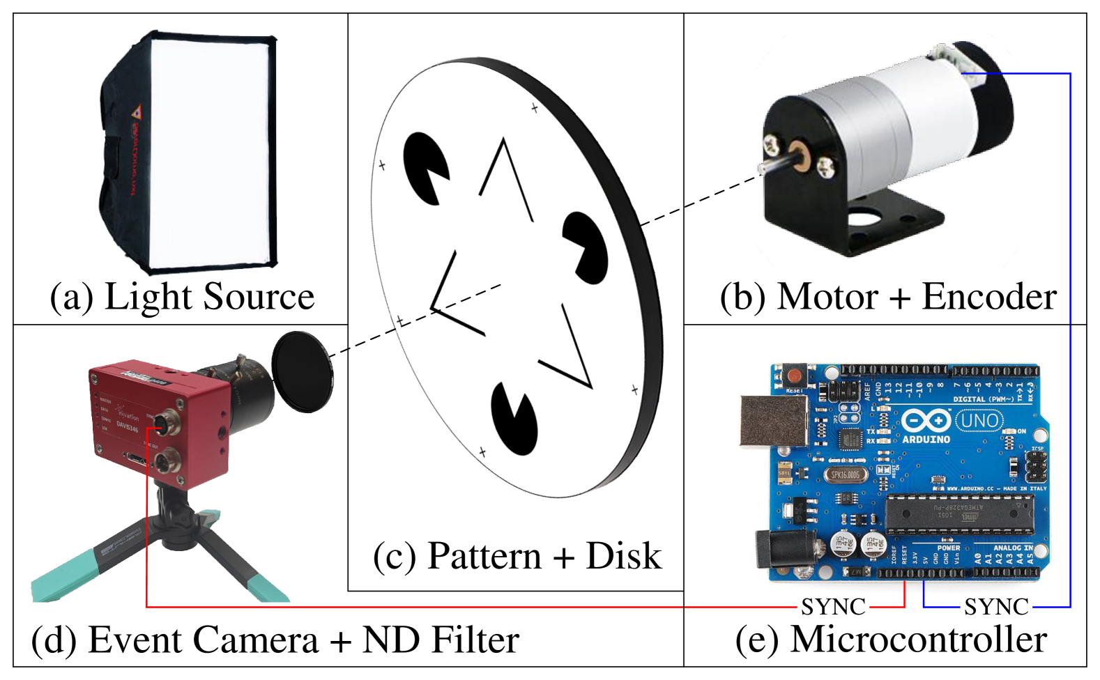
Figure 4: System setup of the proposed event quality evaluation benchmark. An event camera (a) is aiming at the rotating disk with printed patterns attached (c) driven by a motor with a high-precision rotary encoder (b). A light source (a) is placed in front of the disk to provide even and diffused light, and the perceived light is modulated by a neutral density filter for simulating different lighting conditions. To obtain synchronized intensity frames and events, a microcontroller (e) is connected to the motor encoder and event camera to achieve sub-microsecond clock synchronization.

The system setup is presented in Fig. 4. To make the problem as clear as possible, we build our system using scientific control. We use only one high-precision motor to rotate a disk with 10 simple binary textures as shown in Fig. 5. The usage of binary patterns avoids explicit modelling of scene irradiance, and illusory patterns are used to simulate various motion types and speeds. Specifically, the spiral1 (h) and spiral2 (i) patterns are used to generate radial translation motion and others are mainly used to measure the rotary and combined motion types with different speed and pattern complexity. These patterns are printed on board with known dimensions, so once the spatial calibration is done, it’s possible to obtain ground truth intensity frames using the readings from the motor encoder at any time.

The disk is rotated by a motor, which has a high-precision giant magnetoresistance motor encoder to sense the rotor orientation in an event-driven manner. Once the orientation changes above a given threshold, a level jump is sensed on the encoder wires so that the relative angle can be obtained with high time precision. The angular precision of the encoder is 120000 per rotation, resulting in a 0.003°step. The encoder is further calibrated using the aiming laser and a photodiode. The speed of the motor can be controlled using pulse-width modulation to obtain a spinning speed ranging from 0 to 150 revolutions per minute.

To synchronize the motor reading and events, we use a microcontroller to generate synchronization pulses. The synchronization pulses are sent to the Trigger Port of the event camera and can be read from the output with the camera’s internal clocking. The output from the motor encoder is also monitored on the same time base, thus achieving a signal synchronization accuracy of 10ns, much lower than the event timestamp precision of 1$\mu$s so microsecond-level ground-truth intensity frames are available.

Since the quality of events is also affected by the event camera model, two models are used to capture the Rotary Event Dataset (RED):

• DAVIS346 [2] is produced by Inivation and has a spatial resolution of 346$\times$260 and temporal resolution of 1$\mu$s. It uses a custom sensor to also output monochromatic intensity frames at the same time.

• EVK4 [3] is produced by Prophesee and has a spatial resolution of 1280$\times$720 and temporal resolution of 1$\mu$s. It uses an IMX636ES sensor which only outputs events.

Since the quality of captured events is highly-dependent on illumination [32], all the captured sequences are captured under two illumination conditions using a flicker-free lamp, each containing three speed setups, thus making up a total of 60 highly-synchronized event sequences. More details are provided in the supplementary material.

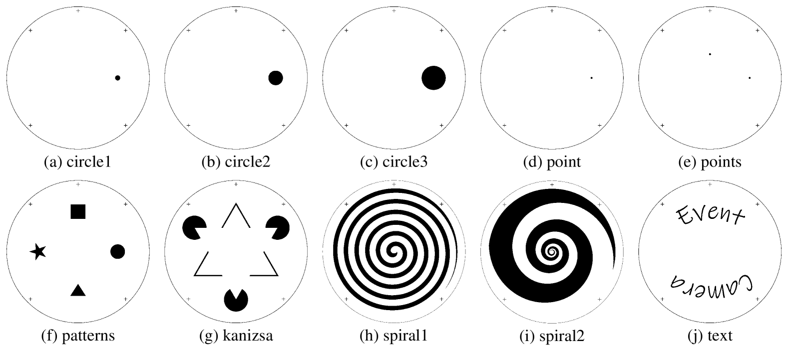
Figure 5: Printed binary patterns used for event quality evaluation. The point (e) and points (f) patterns are only used for evaluating the performance of event-based point tracking.

4 Experiments

In this section, we conduct our main experiments on event signal filtering, super-resolution, and direct blob tracking to analyze the performance and parameter dependency of the proposed EDFilter. These tasks are defined as below:

• Event Signal Filtering aims to output events that authentically reflect real scene radiance change with precise time and amplitude.

• Event Super-Resolution aims to output events with higher resolution that authentically reflect scene irradiance change with precise time and amplitude.

• Event-based Direct Blob Tracking aims to output events that authentically reflect the real blob motion.

4.1 Experimental Settings

Methods. The compared algorithms are:

• Raw is the baseline method that returns raw event stream without filtering.

• EvFlow [20] is a motion-based event denoising method that passes events having reasonable optical flow, which is estimated by local plane fitting. The parameters are selected as $vmax=10p/ms$, $locality=3p\times 3p\times 3ms$.

• Ynoise [18] is a density-based event denoising method that passes events with large event density over a spatiotemporal neighborhood. The parameters are selected as $deltaT=10ms$, $lParam=3$, $threshold=2$;

• MLPF [14] is a timestamp-based event denoising method that uses a 3-layer MLP classification network to output the real probability of each event based on stacked local timesurface input. The discrimination threshold is selected as $realThres=0.5$.

• EventZoom [10] is a frame-based event denoising and interpolation method that uses 3D-UNET to predict denoised and super-resolved event frames. The output events are returned from the output frame by even redistribution within the frame interval. The output threshold parameter is selected as $th=0.5$.

For EDFilter, the parameters are selected as $W=100ms,\gamma=4ms$, LUT keys range from $156.25\mu s$ to $40ms$ with $2\times$ step, $p=2$, $dt=10ms$ for the event signal filtering and super-resolution tasks and $p=1$, $dt=\inf$ or pure asynchronous sampling and interpolation for the event-based direct blob tracking task.

Metrics. Different patterns are used for different tasks. The point and points patterns are only used for event-based point tracking and other patterns are used both for event denoising and event super-resolution. For event signal filtering and super-resolution, each sequence lasts around 20s with variable speed controlled by hand, and we manually select 10s for comparison. Since the proposed method can output any number of events reflecting the same scene dynamics, the evaluation metrics are modified to be unrelated to the exact number of events for fair comparison under different scenarios. The ground-truth radiance change is compared with event density volume, whose interval is selected as 1ms. To make the metric unrelated to the exact number of events, we estimate the best scaling factor during the calculation of Normalized Mean Squared Error (NMSE) as:

$$\small\textrm{NMSE}=\frac{\min_{k}\sum_{p\in\{-1,1\}}\sum_{i}(g_{i,p}-kd_{i,p})^{2}}{\sum_{p\in\{-1,1\}}\sum_{i}g_{i,p}^{2}},$$ (55)

where $g_{i,p}$ is the ground-truth radiance change with polarity $p$ and $d_{i,p}$ is the corresponding event density of polarity $p$. For the event-based direct blob tracking, each sequence lasts around 30s with variable speed controlled by hand, and we manually select 20s for comparison. We use integrated tracking error (ITE) for comparison:

$$\small\textrm{ITE}=\sum_{i}\frac{(t_{i}-t_{i-1})}{T}||(x_{i},y_{i})-(c_{x}(t_{i}),c_{y}(t_{i}))||_{1},$$ (56)

where $(t_{i},x_{i},y_{i})$ is the coordinate of the $i$-th event, $(c_{x}(t_{i}),c_{y}(t_{i}))$ is the coordinate of point center at time $t_{i}$, $T$ is the time span. For the points pattern, each event is compared against the closest point. The usage of integration in Eq. 56 makes the point tracking result independent of the number of output events.

4.2 Main Results

4.2.1 Event Signal Filtering

The results of event signal filtering on NMSE metric are shown in Table I. In summary, the proposed method has the best performance among all other methods except for the text and the kanizsa sequences captured by DAVIS346, where our method ranks the second and the third respectively, demonstrating the proposed method reserves the most precise radiance change information. Aside from that, the standard deviation is reported in the std columns, demonstrating the best robustness among all other methods.

It’s worth noting that the EVK4 model attains higher resolution at the expense of smaller pixel size and is more noisy, represented by the high NMSE in the raw rows, especially when the scene texture is simple, as shown in the circle1, circle2 and circle3 sequences. However, due to its high readout bandwidth, noise events can be suppressed by the overwhelming number of real events, as shown in the kanizsa and text columns. This difference shows that evaluating different event camera models separately is crucial for drawing meaningful conclusions and indicates the difficulty of designing universal event signal filters, which further demonstrates the superiority of the proposed method.

For a more in-depth analysis, visualization of filtered events are shown in Fig. 6. EvFlow is the most aggressive among all other methods that many real events are also removed alongside, so has the worst performance in general. MLPF and Ynoise are also discriminative models but due to the rich information contained in the local timesurface and effective MLP-based discriminator, MLPF usually has the second-best performance by effectively preserving the real spatiotemporal structure within noisy events. The EventZoom column is The EventZoom column is somewhat counterintuitive because it looks good visually but has poor NMSE performance. To explain that, the first thing to note is that it depends on a fixed discretization scheme to construct the input event frames, and output events are evenly distributed in time within the discretization interval, so precise temporal information is lost, as shown in 3D event point clouds. The second problem is that the internal convolutional blocks will definitely cause energy diffusion in space, so radiance change cannot be precisely retained, especially around hotpixels as shown in the top right corner of the Urban sequence. In contrast, the proposed method is able to adapt to the varying scene temporal characteristics by fitting the best temporal kernel against observed events, and spatial sparsity is enforced by exploiting local motion and optimizing the $L_{p}$ reconstruction cost.

We also provide rooted-mean-square error (RMSE) results in the Ref-E [11] dataset for reference, which uses a similar way to ours to generate ground-truth events and compare the generated event frame. As shown in Table II, the proposed method has comparable performance with the previously state-of-the-art method EventZoom.

TABLE I: NMSE results of event signal filtering. DAVIS/EVK columns: DAVIS346 and EVK4 captured sequences. Bold red/blue: 1st/2nd best values.

	circle1		circle2		circle3		kanizsa		patterns		spiral1		spiral2		text		std
Method	DAVIS	EVK	DAVIS	EVK	DAVIS	EVK	DAVIS	EVK	DAVIS	EVK	DAVIS	EVK	DAVIS	EVK	DAVIS	EVK	DAVIS	EVK
Raw	0.106	0.390	0.087	0.166	0.060	0.118	0.061	0.054	0.085	0.087	0.137	0.139	0.094	0.139	0.058	0.052	0.045	0.140
EventZoom[10]	0.223	0.338	0.111	0.109	0.084	0.076	0.210	0.206	0.129	0.129	0.331	0.108	0.120	0.108	0.283	0.227	0.168	0.130
Evflow[20]	0.285	0.504	0.265	0.378	0.242	0.361	0.094	0.212	0.144	0.214	0.529	0.312	0.346	0.312	0.065	0.142	0.198	0.163
MLPF[14]	0.104	0.226	0.091	0.073	0.066	0.054	0.062	0.049	0.089	0.072	0.250	0.094	0.134	0.094	0.057	0.049	0.090	0.057
Ynoise[18]	0.244	0.230	0.186	0.125	0.159	0.072	0.162	0.082	0.173	0.101	0.516	0.115	0.309	0.115	0.187	0.089	0.160	0.068
Ours	0.096	0.193	0.075	0.059	0.055	0.044	0.071	0.043	0.079	0.062	0.121	0.086	0.088	0.086	0.058	0.038	0.036	0.051

TABLE II: RMSE results for the Ref-E [11] dataset. Bold red: best value.

Raw	MLPF[14]	EventZoom[10]	Ours
0.105	0.102	0.087	0.092

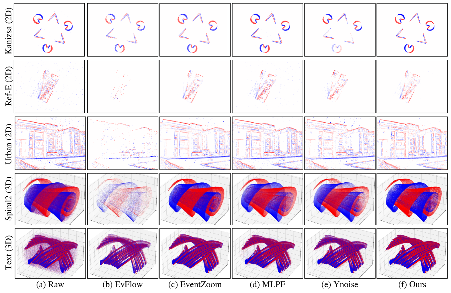
Figure 6: Visualization of filtered events as 2D event frames (top 3 rows) and 3D point clouds (bottom 2 rows). Sequences come from the proposed RED dataset (rows 1,4,5), the Ref-E dataset [11] (row 2) and the ECD dataset [38] (row 3).

4.2.2 Super-Resolution

The results of 2$\times$ super-resolution on NMSE are shown in Table III. The proposed method has the lowest NMSE value for most sequences, and is close to EventZoom for the remaining sequences. It’s exciting to see that ours has such performance just by adapting bilinear interpolation to the asynchronous case from Eq. 41, which shows great potentiality of the proposed framework. Based on the same principle, any target resolution is available by changing the interpolation kernel, making it a common adaptor design for processes that only accept certain spatial resolutions or need a variable setup of computational load.

However, such design has inefficiencies when dealing with the sparse nature of events as shown in real-world sequences in Fig. 7. Diffused density flow is usually expected compared with EventZoom, which implicitly learns to restore scene structure from large-scale training pairs. To that end, a more detailed spatial density flow model is required for complex scenes.

TABLE III: NMSE results of 2$\times$ super-resolution. DAVIS/EVK columns: DAVIS346 and EVK4 captured sequences. Bold red: best value.

	circle1		circle2		circle3		kanizsa		patterns		spiral1		spiral2		text		std
Method	DAVIS	EVK	DAVIS	EVK	DAVIS	EVK	DAVIS	EVK	DAVIS	EVK	DAVIS	EVK	DAVIS	EVK	DAVIS	EVK	DAVIS	EVK
EventZoom[10]	0.190	0.298	0.103	0.077	0.070	0.048	0.174	0.166	0.121	0.102	0.130	0.061	0.077	0.075	0.224	0.160	0.094	0.102
Ours	0.103	0.193	0.078	0.066	0.059	0.056	0.076	0.050	0.087	0.068	0.119	0.075	0.088	0.086	0.055	0.054	0.037	0.050

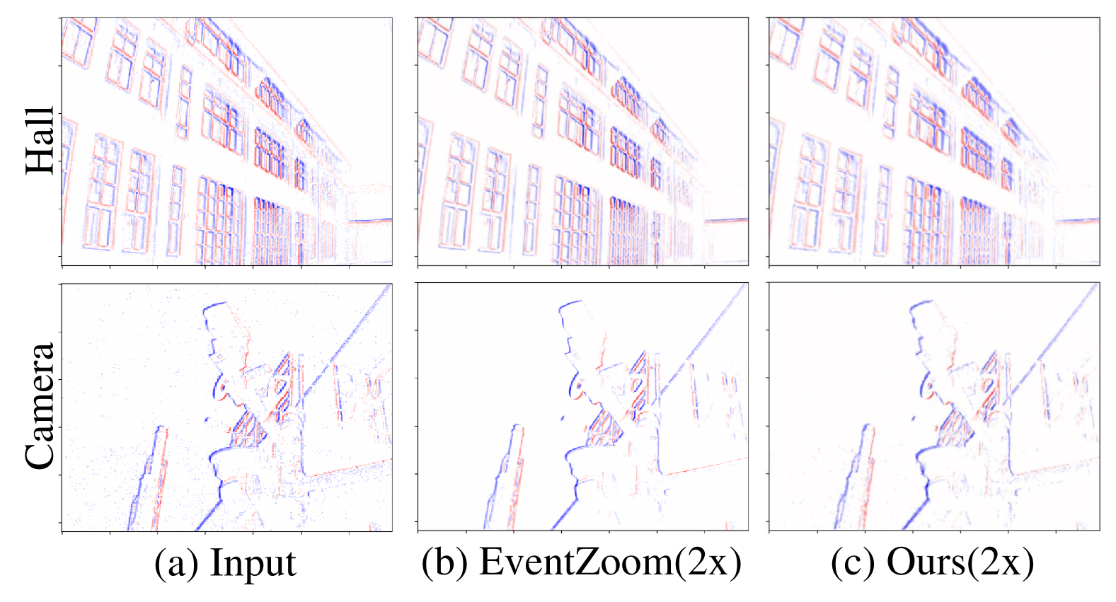
Figure 7: 2$\times$ super-resolution results on the E-MLB[32] dataset.

4.2.3 Direct Blob Tracking

The results of direct blob tracking on ITE are shown in Table IV, where our method performs in the top two among all methods. The only comparable method is EvFlow which is also more stable viewing the lowest standard deviation. However, according to filtering results shown in Section 4.2.1, it has the worst performance in preserving accurate scene irradiance change. From the 3D visualization results shown in Fig. 8, EvFlow only keeps the most representative events along the trajectory, which is beneficial for tracking obvious motions. Such phenomenons indicate that there is an inherent contradiction between accurate scene irradiance perception and motion perception, which is another manifestation of the interaction between the state and process information.

The proposed method performs well on both sides because a physical quantity for a complete event distribution modelling, probability flux density, is derived, and an optimization framework is proposed, filling the gap between separate modelling of the state and process information.

TABLE IV: ITE results in millimeters. DAVIS/EVK columns: DAVIS346 and EVK4 captured sequences. Red/blue: 1st/2nd best values.

	point		points		std
Method	DAVIS	EVK	DAVIS	EVK	DAVIS	EVK
Raw	7.542	46.319	4.711	30.728	1.787	24.665
EventZoom[10]	4.168	4.711	3.680	3.084	2.096	2.672
EvFlow[20]	2.290	2.978	2.306	2.125	0.581	1.071
MLPF[14]	7.005	28.811	4.499	17.444	1.540	11.635
Ynoise[18]	2.805	7.223	3.428	4.444	1.031	7.864
Ours	2.358	2.954	2.518	2.046	0.810	1.297

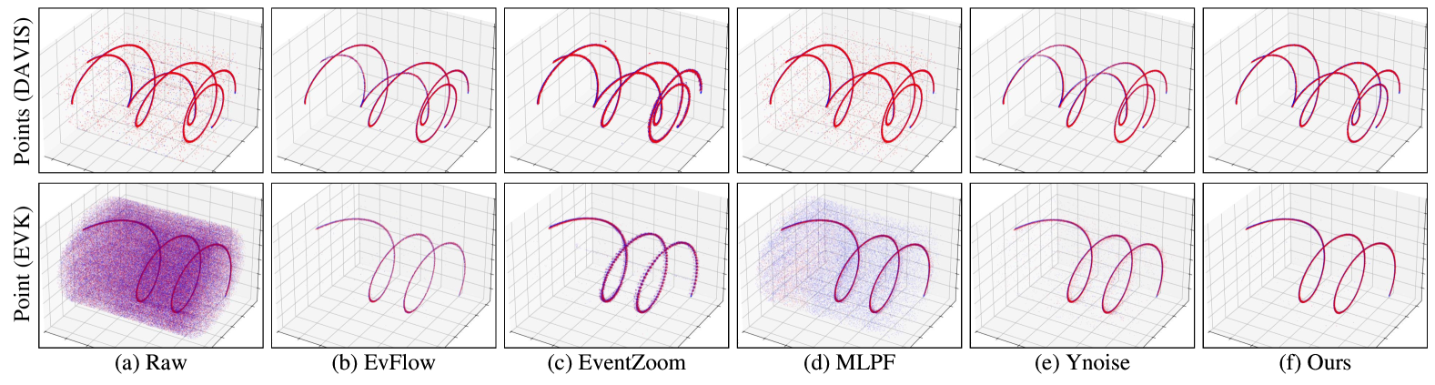
Figure 8: Visualization of filtered events in 3D as point clouds.

4.2.4 Analysis of Different Filtering Components

There are three parts working sequentially to output filtered events, responsible for the temporal modelling, spatial modelling and event sampling, respectively. To find how one part affects another, this section only controls one part to see how the final performance changes. The average performance over all sequences on both the filtering and the direct blob tracking tasks are reported in Fig. 9.

By alternating the temporal part, we can see that the proposed DensityFlow model has the best performance for both the event signal filtering and direct blob tracking tasks. This is more obvious when it comes to accurate motion perception, where the Poisson [29] and Gaussian [21] models are based on a predefined temporal correlation window while the DensityFlow model can adapt to the scene by maximizing the observation likelihood. Regarding the spatial part, differences suggest that L1 is preferred in precise motion perception while L2 is better for maintaining accurate irradiance changes. For the sampling part, asynchronous sampling obviously has the lowest ITE but has higher NMSE than hybrid sampling, as shown in the Async and Compound10ms bars. In fact, it’s generally suggested to be more aggressive when only motion information is required according to the results reported in Section 4.2.3. Pure synchronous sampling has the worst performance in all cases, clearly showing inefficiencies when dealing with asynchronous event signals because, unlike ordinary time series, their occurrence is unpredictable. These results also suggest that even though infinite sampling may be an option to obtain continuous event density flow, the performance may not make such a big difference, especially considering its high computational requirements.

Figure 9: Analysis results on the event signal filtering and direct blob tracking tasks. Blue bars on the top represent the direct blob tracking results in ITE, and yellow ones on the bottom represent the event signal filtering results in NMSE. Temporal part: DensityFlow refers to the proposed temporal sequential model, Poisson [29] means using homogeneous Poisson processes for constructing the density flow, Gaussian [21] means using Gaussian kernels for constructing the density flow. Spatial part: L1 and L2 refer to selecting $p=1$ and $p=2$ in Eq. 35 to update event density, respectively. Sampling part: Async refers to pure asynchronous density flow sampling, SyncT refers to pure synchronous density flow sampling with sampling period selected as $T$, CompoundT refers to hybrid density flow sampling with the synchronous density flow sampling period selected as $T$.

4.2.5 Runtime Analysis

This section shows the runtime performance of the proposed method as a reference for online deployment. One of the main difficulties for such evaluation is the lack of consistent performance metrics due to the different synchronous and asynchronous filter designs. Since events are inherently asynchronous signals, we use two performance metrics to evaluate different aspects of an asynchronous algorithm: latency measures how long it takes to produce an output once one event arrives, tested on an online evaluation setup; throughput measures the average number of events processed over a large time span, tested on an offline evaluation setup. Three representative algorithms, namely MLPF, EventZoom and EDFilter (Ours) are reported based on the same setup with a spatial resolution of events as $346\times 260$ using a single core of R9-7945HX cpu in Table V. For the synchronous algorithm EventZoom, the analogous throughput is calculated on a real event sequence with an average event rate of 1.23Events/$\mu$s. Since we have not yet implemented an offline evaluation procedure for the proposed method, the reported throughput is also tested on an online setup.

TABLE V: Latency and throughput comparison of event signal filters.

Metric	MLPF[14]	EventZoom[10]	Ours
Latency (s)	7.55e-6	1.21e0	4.99e-6
Throughput (Events/s)	4.73e6	1.34e5	2.10e5

The proposed method achieves the lowest latency by an average latency of 4.99$\mu$s from the table, demonstrating the superiority of runtime performance. It even outperforms the discriminative method MLPF by around $51\%$, suggesting that it’s possible to perform complex signal processing for events with such low latency. The synchronous algorithm EventZoom has the highest latency since global information must be accumulated into event frames and then processed by complex video-processing modules. For the throughput performance, it’s encouraging that even without applying specific acceleration techniques for offline deployment, our method can still process around 210kEvents per second, which is even higher than EventZoom. We plan to define a set of highly optimized low-level routines based on the proposed framework for further speedups in the future.

4.3 Applications

One question concerning the effectiveness of a filter is whether downstream applications may benefit from it. This section answers this question by two common applications: Event-Based SLAM and Event-Based Video Reconstruction. They mainly examine the ability of an event signal in motion perception and irradiance perception respectively.

4.3.1 Event-Based SLAM

The reference SLAM algorithm is selected as ESVO [39], which uses a stereo event camera setup of event cameras to generate synchronized timesurfaces and uses stereo semi-global matching to construct camera trajectory along with a sparse global map. The performance is evaluated by comparing the computed trajectories and ground-truth trajectories. The absolute translational error (RMS) values before and after inserting the proposed filter on both event signals are provided in Table VI with the top view of several computed trajectories shown in Fig. 10. It can be seen that after inserting the proposed EDFilter, the tracking performance is improved for most sequences, especially for those having poor results at first like upenn_flying1 and upenn_flying3. This is more obvious in Fig. 10 where the computed trajectories are closer to the ground truth. Such results are a direct demonstration of the motion preservation ability of the proposed method.

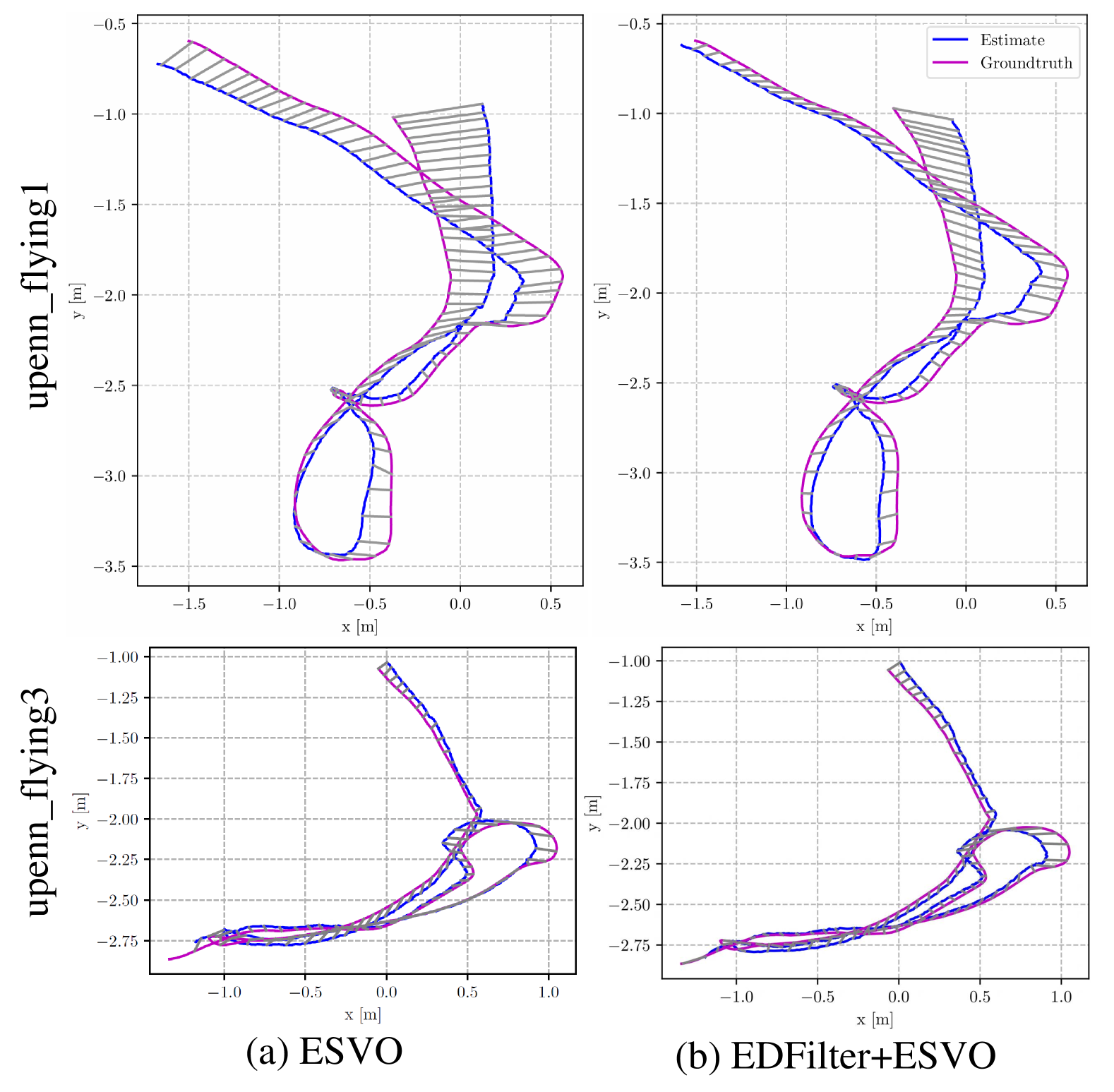
Figure 10: Top view of trajectory compared with ground-truth. Correspondence is shown as gray lines.

TABLE VI: RMS tracking error in centimeters. Bold red: best value.

Method	indoor_ flying1	indoor_ flying3	rpg_ bin	rpg_ boxes	rpg_ desk	rpg_ monitor
ESVO[39]	18.4	10.1	3.0	6.1	3.5	2.3
EDFilter+ESVO[39]	15.5	8.8	2.9	4.8	3.9	2.2

4.3.2 Video Reconstruction

The reference video reconstruction algorithm is selected as E2VID [40], which learns to generate corresponding video frames from input event frames with a recurrent network. As with evaluating other data preprocessing pipelines, we regenerate processed events and then fine-tune the pretrained model to obtain the final reconstruction results. The performance is assessed on the E-MLB [32] dataset which contains 1200 paired event sequences under varying degradation conditions. The average peak-to-signal-ration (PSNR), mean-square error (MSE), structural similarity (SSIM) index and perceptual similarity (LPIPS) [41] are reported in Table VII with several reconstructed frames shown in Fig. 11. From Table VII, the reconstruction performance has been improved by much for all the metrics after inserting the proposed filter. As shown on the Books and Shapes_Day sequences, the reconstructed frame is cleaner than before while on the Toys and Stairs sequences, more scene details are reconstructed. Such results clearly demonstrate the benefit of the proposed filter.

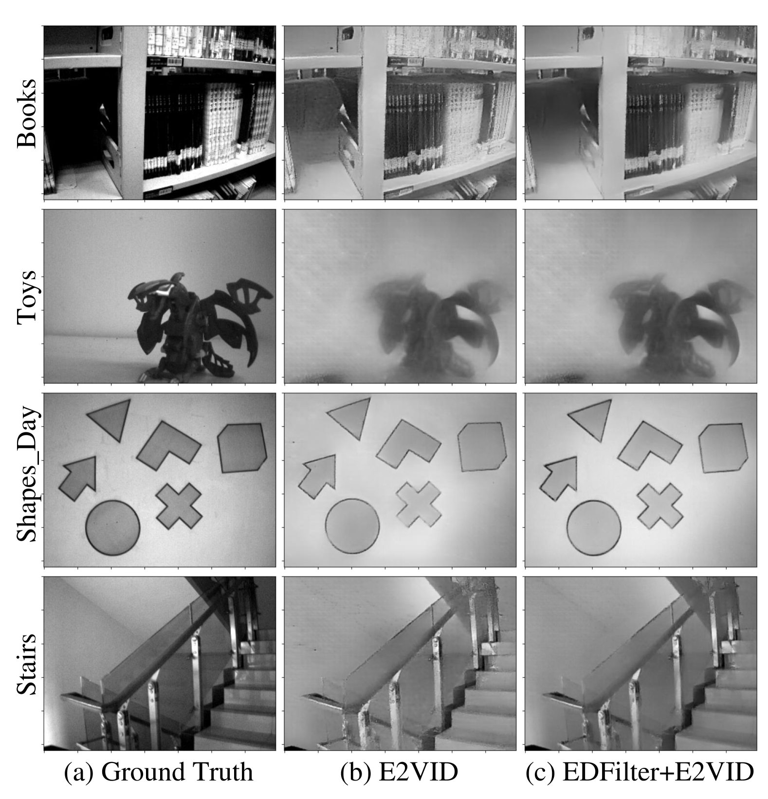
Figure 11: Visualization of reconstructed frames on several sequences on the E-MLB [32] dataset.

TABLE VII: E-MLB [32] video reconstruction results. Bold red: best value.

Method	PSNR$\uparrow$	MSE$\downarrow$	SSIM$\uparrow$	LPIPS$\downarrow$
E2VID[40]	16.04	0.035	0.53	0.30
EDFilter+E2VID[40]	18.37	0.019	0.68	0.24

5 Conclusion

This paper presents a novel event signal filtering framework called Event Density Flow Filter (EDFilter) in a generative way, where event correlation is modelled by estimating continuous probability flux derived from the irradiance intensity diffusion process. Nonparametric kernel smoothing methods are proposed to construct the discrete event density flow values from discrete event signals adaptively by maximizing the event observation likelihood in time and minimizing the motion-guided local reconstruction error in space, then filtered events can be generated back by sampling and interpolating the continuous event density flow. A real-world benchmark dataset containing microsecond-level ground-truth scene irradiance under varying capturing conditions is also provided as the Rotary Event Dataset (RED), which enables full-reference evaluation on three main tasks, including event signal filter, super-resolution, and direct event-based blob tracking. Extensive experiments on the three main tasks and further downstream applications including SLAM and video reconstruction demonstrate the superiority of the proposed filter.

References

- [1] P. Lichtsteiner, C. Posch, and T. Delbruck, “A 128 128 120 db 15s latency asynchronous temporal contrast vision sensor,” IEEE journal of solid-state circuits, vol. 43, no. 2, pp. 566–576, 2008.
- [2] G. Taverni, D. P. Moeys, C. Li, C. Cavaco, V. Motsnyi, D. S. S. Bello, and T. Delbruck, “Front and back illuminated dynamic and active pixel vision sensors comparison,” IEEE Transactions on Circuits and Systems II: Express Briefs, vol. 65, no. 5, pp. 677–681, 2018.
- [3] T. Finateu, A. Niwa, D. Matolin, K. Tsuchimoto, A. Mascheroni, E. Reynaud, P. Mostafalu, F. Brady, L. Chotard, F. LeGoff et al., “5.10 a 1280 720 back-illuminated stacked temporal contrast event-based vision sensor with 4.86 m pixels, 1.066 geps readout, programmable event-rate controller and compressive data-formatting pipeline,” in 2020 IEEE International Solid-State Circuits Conference-(ISSCC). IEEE, 2020, pp. 112–114.
- [4] G. Gallego, H. Rebecq, and D. Scaramuzza, “A unifying contrast maximization framework for event cameras, with applications to motion, depth, and optical flow estimation,” in Proceedings of the IEEE conference on computer vision and pattern recognition, 2018, pp. 3867–3876.
- [5] A. R. Vidal, H. Rebecq, T. Horstschaefer, and D. Scaramuzza, “Ultimate slam? combining events, images, and imu for robust visual slam in hdr and high-speed scenarios,” IEEE Robotics and Automation Letters, vol. 3, no. 2, pp. 994–1001, 2018.
- [6] D. Falanga, K. Kleber, and D. Scaramuzza, “Dynamic obstacle avoidance for quadrotors with event cameras,” Science Robotics, vol. 5, no. 40, p. eaaz9712, 2020.
- [7] G. Gallego, T. Delbrück, G. Orchard, C. Bartolozzi, B. Taba, A. Censi, S. Leutenegger, A. J. Davison, J. Conradt, K. Daniilidis et al., “Event-based vision: A survey,” IEEE transactions on pattern analysis and machine intelligence, vol. 44, no. 1, pp. 154–180, 2020.
- [8] Y. Nozaki and T. Delbruck, “Temperature and parasitic photocurrent effects in dynamic vision sensors,” IEEE Transactions on Electron Devices, vol. 64, no. 8, pp. 3239–3245, 2017.
- [9] Y. Hu, S.-C. Liu, and T. Delbruck, “v2e: From video frames to realistic dvs events,” in Proceedings of the IEEE/CVF Conference on Computer Vision and Pattern Recognition, 2021, pp. 1312–1321.
- [10] P. Duan, Z. W. Wang, X. Zhou, Y. Ma, and B. Shi, “Eventzoom: Learning to denoise and super resolve neuromorphic events,” in Proceedings of the IEEE/CVF Conference on Computer Vision and Pattern Recognition, 2021, pp. 12 824–12 833.
- [11] P. Duan, Y. Ma, X. Zhou, X. Shi, Z. W. Wang, T. Huang, and B. Shi, “Neurozoom: Denoising and super resolving neuromorphic events and spikes,” IEEE Transactions on Pattern Analysis and Machine Intelligence, 2023.
- [12] C. Zhang, X. Zhang, M. Lin, C. Li, C. He, W. Yang, G.-S. Xia, and L. Yu, “Crosszoom: Simultaneously motion deblurring and event super-resolving,” arXiv preprint arXiv:2309.16949, 2023.
- [13] W. Weng, Y. Zhang, and Z. Xiong, “Boosting event stream super-resolution with a recurrent neural network,” in European Conference on Computer Vision. Springer, 2022, pp. 470–488.
- [14] S. Guo and T. Delbruck, “Low cost and latency event camera background activity denoising,” IEEE Transactions on Pattern Analysis and Machine Intelligence, vol. 45, no. 1, pp. 785–795, 2022.
- [15] Z. W. Wang, P. Duan, O. Cossairt, A. Katsaggelos, T. Huang, and B. Shi, “Joint filtering of intensity images and neuromorphic events for high-resolution noise-robust imaging,” in Proceedings of the IEEE/CVF Conference on Computer Vision and Pattern Recognition, 2020, pp. 1609–1619.
- [16] R. Baldwin, M. Almatrafi, V. Asari, and K. Hirakawa, “Event probability mask (epm) and event denoising convolutional neural network (edncnn) for neuromorphic cameras,” in Proceedings of the IEEE/CVF Conference on Computer Vision and Pattern Recognition, 2020, pp. 1701–1710.
- [17] T. Delbruck et al., “Frame-free dynamic digital vision,” in Proceedings of Intl. Symp. on Secure-Life Electronics, Advanced Electronics for Quality Life and Society, vol. 1. Citeseer, 2008, pp. 21–26.
- [18] Y. Feng, H. Lv, H. Liu, Y. Zhang, Y. Xiao, and C. Han, “Event density based denoising method for dynamic vision sensor,” Applied Sciences, vol. 10, no. 6, p. 2024, 2020.
- [19] P. Zhang, Z. Ge, L. Song, and E. Y. Lam, “Neuromorphic imaging with density-based spatiotemporal denoising,” IEEE Transactions on Computational Imaging, 2023.
- [20] Y. Wang, B. Du, Y. Shen, K. Wu, G. Zhao, J. Sun, and H. Wen, “Ev-gait: Event-based robust gait recognition using dynamic vision sensors,” in Proceedings of the IEEE/CVF Conference on Computer Vision and Pattern Recognition, 2019, pp. 6358–6367.
- [21] J. Li, Y. Fu, S. Dong, Z. Yu, T. Huang, and Y. Tian, “Asynchronous spatiotemporal spike metric for event cameras,” IEEE Transactions on Neural Networks and Learning Systems, 2021.
- [22] H. Liu, C. Brandli, C. Li, S.-C. Liu, and T. Delbruck, “Design of a spatiotemporal correlation filter for event-based sensors,” in 2015 IEEE International Symposium on Circuits and Systems (ISCAS). IEEE, 2015, pp. 722–725.
- [23] A. Khodamoradi and R. Kastner, “ o (n)-space spatiotemporal filter for reducing noise in neuromorphic vision sensors,” IEEE Transactions on Emerging Topics in Computing, vol. 9, no. 1, pp. 15–23, 2018.
- [24] E. Mueggler, C. Forster, N. Baumli, G. Gallego, and D. Scaramuzza, “Lifetime estimation of events from dynamic vision sensors,” in 2015 IEEE international conference on Robotics and Automation (ICRA). IEEE, 2015, pp. 4874–4881.
- [25] P. Duan, Z. W. Wang, B. Shi, O. Cossairt, T. Huang, and A. K. Katsaggelos, “Guided event filtering: Synergy between intensity images and neuromorphic events for high performance imaging,” IEEE Transactions on Pattern Analysis and Machine Intelligence, vol. 44, no. 11, pp. 8261–8275, 2021.
- [26] R. Graça, B. McReynolds, and T. Delbruck, “Shining light on the dvs pixel: A tutorial and discussion about biasing and optimization,” in Proceedings of the IEEE/CVF Conference on Computer Vision and Pattern Recognition, 2023, pp. 4044–4052.
- [27] Z. Wang, Y. Ng, C. Scheerlinck, and R. Mahony, “An asynchronous kalman filter for hybrid event cameras,” in Proceedings of the IEEE/CVF International Conference on Computer Vision, 2021, pp. 448–457.
- [28] X. Liu, M. Cheng, D. Shi, and L. Shi, “Towards event-based state estimation for neuromorphic event cameras,” IEEE Transactions on Automatic Control, 2022.
- [29] C. Gu, E. Learned-Miller, D. Sheldon, G. Gallego, and P. Bideau, “The spatio-temporal poisson point process: A simple model for the alignment of event camera data,” in Proceedings of the IEEE/CVF International Conference on Computer Vision, 2021, pp. 13 495–13 504.
- [30] S. Lin, Y. Ma, Z. Guo, and B. Wen, “Dvs-voltmeter: Stochastic process-based event simulator for dynamic vision sensors,” in European Conference on Computer Vision. Springer, 2022, pp. 578–593.
- [31] V. Padala, A. Basu, and G. Orchard, “A noise filtering algorithm for event-based asynchronous change detection image sensors on truenorth and its implementation on truenorth,” Frontiers in neuroscience, vol. 12, p. 118, 2018.
- [32] S. Ding, J. Chen, Y. Wang, Y. Kang, W. Song, J. Cheng, and Y. Cao, “E-mlb: Multilevel benchmark for event-based camera denoising,” IEEE Transactions on Multimedia, 2023.
- [33] B. Oksendal, Stochastic differential equations: an introduction with applications. Springer Science & Business Media, 2013.
- [34] A. Klenke, Probability theory: a comprehensive course. Springer Science & Business Media, 2013.
- [35] F. Gesztesy, R. Nichols, and M. Zinchenko, Sturm? Liouville Operators, Their Spectral Theory, and Some Applications. American Mathematical Society, 2024, vol. 67.
- [36] I. Rubin, “Regular point processes and their detection,” IEEE Transactions on Information Theory, vol. 18, no. 5, pp. 547–557, 1972.
- [37] J. Mattingley and S. Boyd, “Cvxgen: A code generator for embedded convex optimization,” Optimization and Engineering, vol. 13, pp. 1–27, 2012.
- [38] E. Mueggler, H. Rebecq, G. Gallego, T. Delbruck, and D. Scaramuzza, “The event-camera dataset and simulator: Event-based data for pose estimation, visual odometry, and slam,” The International journal of robotics research, vol. 36, no. 2, pp. 142–149, 2017.
- [39] Y. Zhou, G. Gallego, and S. Shen, “Event-based stereo visual odometry,” IEEE Transactions on Robotics, vol. 37, no. 5, pp. 1433–1450, 2021.
- [40] H. Rebecq, R. Ranftl, V. Koltun, and D. Scaramuzza, “High speed and high dynamic range video with an event camera,” IEEE transactions on pattern analysis and machine intelligence, vol. 43, no. 6, pp. 1964–1980, 2019.
- [41] R. Zhang, P. Isola, A. A. Efros, E. Shechtman, and O. Wang, “The unreasonable effectiveness of deep features as a perceptual metric,” in Proceedings of the IEEE conference on computer vision and pattern recognition, 2018, pp. 586–595.