Modular Control of Discrete Event System for Modeling and Mitigating Power System Cascading Failures
Abstract
Cascading failures in power systems caused by sequential tripping of components are a serious concern as they can lead to complete or partial shutdowns, disrupting vital services and causing damage and inconvenience. In prior work, we developed a new approach for identifying and preventing cascading failures in power systems. The approach uses supervisory control technique of discrete event systems (DES) by incorporating both on-line lookahead control and forcible events. In this paper, we use modular supervisory control of DES to reduce computation complexity and increase the robustness and reliability of control. Modular supervisory control allows us to predict and mitigate cascading failures in power systems more effectively. We implemented the proposed control technique on a simulation platform developed in MATLAB and applied the proposed DES controller. The calculations of modular supervisory control of DES are performed using an external tool and imported into the MATLAB platform. We conduct simulation studies for the IEEE 30-bus, 118-bus and 300-bus systems, and the results demonstrate the effectiveness of our proposed approach.
Index Terms:
Discrete event systems, hybrid systems, supervisory control, modular control, on-line control, power systems, cascading failuresI Introduction
Cascading failures in power systems are a significant concern due to the interconnected nature of electrical grids and the potential for a localized issue to propagate and cause widespread outages. The causes of cascading failures include (1) overloading of transmission lines or transformers, (2) voltage instability, (3) equipment failures, (4) natural disasters, (5) cyberattacks, and more.
Because they can lead to widespread blackouts, disrupt vital services and cause significant economical and social losses, cascading failures have been investigated extensively in the literature from different points of view. Among the papers published, the ones using abstracted and higher-level models are most relevant to our work as described below. Influence graphs are used to investigate the probability functions of the initial outages of branches and the outages that occur consequently in [1]. In [2], transition probabilities between states in automata representing components of power systems were formalized. Information about the most vulnerable lines using Markovian models was analyzed in [3] based on line outage data. In [4] and [5], transmission line failure propagation is characterized using a network graph structure. Two cases are considered: when the network remains connected after a contingency and when the failure propagation separates the network into multiple islands.
Graph theory is used in [6, 7] to describe the relationship between initiating events and barriers, system states, and consequences [6], and to analyze the vulnerability of power systems with renewable energy sources [7]. A quantitative assessment that includes a resilience assessment index based on cascading failure graph is provided in [8]. Structural deformation of the graph characteristics of the power system is studied with topological data analysis in [9]. A method is proposed in [10] to identify vulnerable branches by taking into account the propagation characteristics of the cascading failure. A tree partitioning method based on the assumption that a given power system can be represented as a connection of clusters is proposed to mitigate cascading failure [11]. A distributed model based predictive control to mitigate cascading failure risk is proposed in [12]. Network failures initiated by link failures and overloads are studied in [13]. A failure propagation mechanism is described based on a hypergraph model in [14].
Many approaches have been proposed to analyze, model, and control power systems under various scenarios. One approach that considers reducing communication burden, increasing reliability, improving efficiency, and reducing computational load is by using an event-based approach to monitor and control the power system. In [15], the authors performed a survey on modeling methods of cyber-physical power systems. One of the modeling approaches was the use of finite-state machines and event-based models. The authors in [16] proposed an event-triggered load frequency control based on model-free adaptive control, which depends on the system data. In [17], the authors proposed a dynamical event-triggered controller that reduces the usage of communication resources to control multi-area wind power systems under dual alterable aperiodic denial-of-service attacks. The authors in [18] proposed a rule-based supervisory control system to avoid the state of charge violations in a hybrid energy storage system. The authors in [19] proposed a hybrid event-triggered control approach that has both continuous and discrete dynamics to describe the dynamics of power systems under denial of service attacks. In [20], the authors proposed a probabilistic proactive strategy to enhance power system resilience against wildfires that is based on Markov decision process, where the system is represented as states, with events that trigger the transition from one state to another.
Cascading failures in power systems can be viewed as a string of events leading to widespread disruptions or outages. To investigate cascading failures, it is natural to model a system as a discrete event system (DES) at some level of abstraction. Controllers in DES are also called supervisors (we use controller and supervisor interchangeably) and control is called supervisory control [21, 22, 23]. We have proposed a framework using DES and supervisory control to model and mitigate cascading failure processes in [24, 25, 26]. The framework is as follows. To construct a DES model for a power system, we first model its components as automata. Since these automata are small, they can be easily obtained. We then combine these automata using parallel composition to obtain the automaton for the entire power system. Because the parallel composition can be performed by existing DES software, it can be done automatically by computers.
Since some events, such as line trips, cannot be disabled but can be preempted by forcing some forcible events such as load shedding, the conventional supervisory control of DES is not adequate to deal with cascading failures in power systems. We extend supervisory control of DES to include forcible events in [24, 25, 26], which not only provides a solution to the cascading failure problems, but also significantly increases the applicability of supervisory control. To manage computational complexity, we propose an online lookahead control, which significantly reduces the number of states to be considered. We also implement the proposed online lookahead control in an implementation platform using MATLAB. The platform uses MATPOWER to simulate a power system and then control it using the proposed DES controller. Simulation studies are carried out for IEEE 6-, 30-, and 118-bus systems. The results verify the effectiveness of the previously proposed framework.
To control large power systems, the centralized control proposed in [24, 25, 26] may not be adequate, because of large number of states involved. A modular/decentralized control that divides the system and control task into several sub-systems and sub-tasks, each achieved by a local controller, is more appropriate for large power systems for the following reasons. (1) Preventing cascading failures is a time-critical task. Due to large number of states involved, it may take a centralized controller too long to calculate the needed control. (2) A centralized controller may not be robust to communication delays and losses, which are unavoidable. Hence, it is better to have a set of local and decentralized controllers with much smaller communication delays and losses to prevent cascading failures.
Modular supervisory control of DES without forcible events has been investigated in the literature [27, 28, 29, 30]. They have also been applied to manufacturing systems [31], freeway traffic control [32], and multiple UAVs [33]. These applications show that modular supervisory control can make a significant difference in terms of computational complexity and robustness.
To use modular control for preventing cascading failures, we first need to extend conventional modular supervisory control to allow forcible events. Therefore, in this paper, we formally define a modular supervisory control mechanism with forcible events. We then investigate the behavior (language) generated by the modular supervised system. We derive a necessary and sufficient condition for the existence of modular controllers, which is F-controllability and conditional decomposability. If the conditions are satisfied, we will design the modular controllers. If the conditions are not satisfied, then we will design the modular controllers that generate a smaller language and hence ensure no cascading failures in the controlled system, while, at the same time, giving the controlled system maximum freedom to achieve other control objectives.
After developing the theoretical framework for modular supervisory control with forcible events, we implement the results in large scale power systems. The implementation combines two simulation platforms based on [34] and [35] to model and mitigate cascading failures in power systems.
The main innovations and contributions of the paper are as follows. (1) We extend the theory of supervisory control with forcible events from centralized control to modular (decentralized) control. This extension significantly reduces the computational complexity and increases robustness and reliability. (2) Using this extension, we propose a new control method to prevent cascading failures in large scale power. This new method uses modular controllers that make control decisions based on the information received from neighboring nodes and send control actions to the local nodes, making the control faster and more reliable. (3) We develop a new platform based on MATLAB environment that combines discrete-events and continuous-variable parts to implement the proposed modular control. (4) Using the platform, we implement and simulate modular control for the IEEE 30-bus, 118-bus, and 300-bus systems. The results show that the proposed method is highly effective.
The remainder of the paper is organized as follows. Section II introduces DES and necessary notations. Section III discusses supervisory control with forcible events and reviews the findings of [25]. Section IV presents the modular supervisory control theory with forcible events. Section V applies the results to large scale power systems to prevent cascading failures by implementing the modular controllers using the proposed implementation platform. Section V also presents simulation results, which show that the modular supervisory control is effective. The conclusion is drawn in Section VI.
II Discrete Event System Model of Power Systems
A power system to be controlled, called plant, can be modeled as a discrete event system using the following automaton model:
where is the set of states; is the set of events; is the (partial) transition function; and is the initial state. Examples of automata for power line, generator, and load are shown in Section V (Fig. 3).
An automaton can be thought of as a system model with states that represent the operational modes of a given system and events that represent the instantaneous transitions from one state to another. Starting from the initial state , the system continuously moves from one state to another, generating a string of events. Hence, a trajectory of the system is represented by the corresponding string. The automaton model describes the set of all possible trajectories or strings, which is called the language generated by the automation111The terminologies come from automata and formal languages theory, where alphabets represent events, sentences represent strings and languages represent the set of strings. .
Formally, the transition function describes the “dynamics” of the system in the sense that if the current state is and event is defined in , then after the occurrence of , the next state is . can be extended from events to strings as , where denotes the set of all strings over . It is possible that not all events can occur in a state (for example, a switch cannot be turned on again if it is already on). Hence, is a partial function. The language generated by is the set of all strings defined in the automaton starting at the initial state and is denoted by
| (2) |
where is used to denote that is defined.
To obtain an automaton model for a power system, we use a modular approach by first developing (simple) models for its components as
In this paper, we consider transmission lines, generators and loads as the basic components of the power system. See Section V for details. If a power system has transmission lines, generators, and loads, the power system will have components. The overall power system can be constructed using parallel compositions [36]:
| (4) |
The number of states in can increase exponentially with the number of components. In other words, if each component has 2 states, then will have states. To overcome this state explosion, on-line lookahead control and/or modular control can be used to significantly reduce the number of states to be considered. We investigated on-line lookahead control in [25]. In this paper, we investigate modular on-line lookahead control with forcible events.
The computational complexity of control is proportional to the number of states in . For centralized control, this number is . For modular control, since each controller controls a small portion of , this number is , where , , are numbers of transmission lines, generators, and loads controlled by controller , respectively. Clearly, is much smaller than . Therefore, modular control can significantly reduce the computational complexity.
III Supervisory Control with Forcible Events
In control of DES, controllers are also called supervisors (we use controller and supervisor interchangeably) and the control is called supervisory control. In conventional supervisory control, a supervisor can only enable and disable events, it cannot force events. In [25], we extended the conventional supervisory control of DES to allow forcible events since disablement and enablement are not sufficient in our application in power systems. In this section, we briefly review the findings. The controller proposed in [25] can force events in addition to disabling and enabling events to achieve the control objectives. The following assumptions are made on the events.
-
1.
There is a set of controllable events ; that is, their occurrences can be disabled. The set of uncontrollable events are denoted by .
-
2.
There is a set of forcible events ; that is, a controller can force them to occur. We assume that forcible events can preempt uncontrollable events.
In our application of preventing cascading failures in power systems, overloading of transmission lines are uncontrollable. Load shedding is a forcible events. So, for example, transmission line overloading can be prevented by load shedding.
Formally, a controller is a mapping
| (6) |
where denotes the set of all subsets of . Hence, after the occurrence of a string , the events in can occur next.
We use to denote the language generated by the controlled system, which is defined recursively as
| (10) |
After the occurrence of any string , the control must satisfy one of the following two conditions:
-
1.
all events disabled are controllable, that is, , where ; or
-
2.
some events enabled are forcible, that is, . This is based on the assumption that forcible events can preempt uncontrollable events.
Therefore, the following condition is required:
| (13) |
Let be a specification language that excludes all strings leading to cascading failures in power systems. Our goal is to design a controller such that if possible, and , otherwise. Note that means that the controlled system will not generate any strings not in , that is, there will be no cascading failures.
To derive a necessary and sufficient condition for the existence of a controller such that , F-controllability is introduced in [25]: A language is F-controllable with respect to , , and if
| (16) |
F-controllability says that if is not allowed after , then either is controllable (so that it can be disabled) or there is another forcible event that is allowed and can preempt . If , then F-controllability reduces to controllability [21].
The following result is then obtained in [25]: There exists a controller such that if and only if is F-controllable (with respect to , , and ) 222[25] considers partial observation (that is, not all events are observable). Therefore, observability [22] is also required. Since we consider full observation in this paper, observability is not required..
The specification language is often generated by a sub-automaton , that is, for some
where and ( means restricted to ). In this way, the state set is partitioned into legal/safe state set and illegal/unsafe state set .
If is F-controllable, then the following controller achieves , that is, .
| (18) |
If is not F-controllable, then we would like to find a sublanguage of that is F-controllable and to design a controller such that . To give the controlled system maximum freedom to perform other tasks, we would like to make as large as possible. In other words, we would like to find the supremal (largest) F-controllable sublanguage of , denoted by . By our result in [25], exists and is unique, because the union of F-controllable languages is also F-controllable.
can be obtained by iteratively removing “bad” states in . A state is bad if
| (21) |
Denote the automaton after removing all bad states as
where . Then . Clearly, and . Note that if is F-controllable, then and . The controller achieves is given by
| (23) |
Since , ensures that the controlled system stays within the legal specification language ; that is, it can prevent cascading failures. Furthermore, since is the supremal F-controllable sublanguage of , gives the system maximum freedom without violating legal specification, that is, it will not disable/preempt an event unless it is absolutely necessary to do so (not disabling/preempting it will lead to cascading failures).
Constructing off-line requires that we construct first. Since is the parallel composition of all components , the number of states in can grow exponentially with respect to the number of components. To overcome this state explosion problem, we propose on-line control using limited lookahead policies in [25]. For on-line control, we construct a lookahead tree until the number of steps/levels reaches , the limit on lookahead steps. The limited lookahead tree from the current state is denoted by
IV Modular supervisory control with forcible events
For large scale power systems, the centralized control proposed in [25] may not be effective for the following reasons. (1) The complexity of the lookahead tree and hence the time needed to compute the control increases as the number of components increases. Since preventing cascading failures is a time-critical task, it may take a centralized controller too long to compute the control. (2) The centralized controller requires each node in a power system to communicate its information to the central controller, which may not be the most reliable because it has a single point of failure. (3) Communication delays and losses are much more between a centralized controller and distributed actuators than those between local controllers and actuators. As a result, a centralized controller is less robust and reliable.
To overcome the disadvantages of centralized supervisory control, modular supervisory control has been proposed for DES. In modular supervisory control, the uncontrolled system and control tasks are divided into several sub-systems and sub-tasks. Control is then achieved using several modular controllers, each for a sub-system and a sub-task.
Modular supervisory control is more robust and reliable for large scale power systems. However, in order to use modular supervisory control in power systems, we need to extend modular supervisory control to allow forcible events. We will do so in this section.
For modular supervisory control, we assume that the uncontrolled system is the parallel composition of sub-systems, that is,
| (25) |
Note that may itself be the parallel composition of some components , that is, . Denote as
For sub-system , its local forcible events are denoted by ; its local controllable events are denoted by ; and its local uncontrollable events are denoted by , . We assume that all events are observable. Denote the projection from the global events to local events by . Control is achieved by modular controllers
The controlled sub-systems are denoted by . The language generated by the controlled sub-system, denoted by , is defined recursively as
| (29) |
The overall control is the conjunction of all modular controllers, denoted by , that is, for any ,
| (33) |
In other words, an event is allowed () if it is allowed by all controllers () whose event set includes ().
The closed-loop system under modular control is denoted by , which is shown in Fig. 1.

Similar to centralized control, we require that, for all ,
| (36) |
where . To ensure that any event forced by is actually allowed, we further require that, for all ,
| (39) |
Remark 1
Unlike centralized control, where a forcible event can only be forced by one (centralized) controller, in modular control, a forcible event may be forced by more than one (modular) controller. Equation (39) ensures that we can take the disjunction of the set of events forced by modular controllers as the set of forced events. In fact, whichever event is first forced by a modular controller will occur.
Theorem 1
The language generated by the closed-loop system, is given by
| (42) |
Proof
Clearly,
| (49) |
Hence, we need to prove that, for all ,
| (53) |
We prove this by induction of the length of as follows.
Induction Base: Since and , for , that is, , we have
| (57) |
Induction Hypothesis: Assume that for all , ,
| (61) |
Induction Step: We show that for all , , ,
| (65) |
Indeed,
Note that
| (68) |
can also be written as
| (70) |
Assume that is conditionally decomposable [37] in the following sense:
Then, we have the following theorem.
Theorem 2
There exists modular controllers , such that
| (73) |
if and only if is F-controllable with respect to , , and , for .
Proof
(IF) Suppose that is F-controllable with respect to , , and . Then, there exists modular controllers such that , for . By Theorem 1,
| (79) |
Furthermore,
| (81) |
(ONLY IF) Assume that there exist modular controllers , such that
| (84) |
By Theorem 1,
| (89) |
Since by the assumption, we have
Therefore, is F-controllable with respect to , , and , for .
Let us assume that is generated by a sub-automaton , that is, for some
where and .
We use the methods similar to those proposed in the previous section (with replaced by ) to obtain
Consider the following modular controllers, for ,
| (92) |
Theorem 3
The modular controllers , , of Equation (92), ensure the safety of the controlled system, that is,
| (95) |
Proof
Let us first prove that, for all ,
| (97) |
by induction on the length of as follows.
Induction Base: Since and , for , that is, , we have
| (99) |
Induction Hypothesis: Assume that for all , ,
| (101) |
Induction Step: We show that for all , , ,
| (103) |
Indeed,
Since , we have
| (105) |
Furthermore, by Theorem 1,
| (111) |
Modular controllers with a limited lookahead policy of steps, denoted by , can be used to implement similar to the implementation of by .
For better references and explanations, Table 1 summarizes and explains the main notations and symbols used in this paper.
| Notation/symbol | Explanation |
|---|---|
| Plant automaton | |
| Safe/legal/desired language, | |
| also called the specification | |
| Supervisor/controller | |
| Automaton that generates language , | |
| that is, . | |
| Supremal F-controllable sublanguage of | |
| Automaton that generates language | |
| Supervisor/controller that achieves | |
| The language generated by the supervised system | |
| Automaton of component | |
| Automaton of sub-system | |
| Safe/legal/desired language of sub-system | |
| Automaton that generates language | |
| Supremal F-controllable sublanguage of | |
| Automata that generates language | |
| Supervisor/controller that achieves | |
| The language generated by the supervised | |
| sub-system | |
| The language generated by the supervised system | |
| with modular controllers |
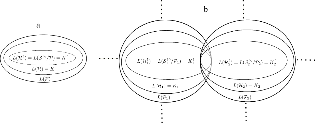
The relations among languages discussed earlier are shown in Fig. 2 as a subset diagrams for both centralized control and modular control.
V Implementation and Simulations
We implement and simulate the modular controllers for power systems to mitigate cascading failures in this section. We first construct the sub-system model for each node based on the components connected to it and its neighboring nodes. These components are: generators, transmission lines, and loads. In this paper, we only consider the neighboring nodes connected directly by a transmission line to the node of interest to construct a controller.
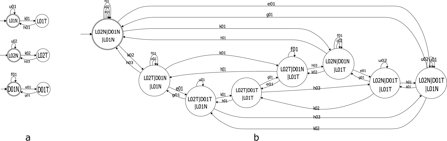
The automaton for transmission lines is shown in Fig. 3.
It has two states, normal (N) and tripped (T), and three events, which are
: Line is tripped,
: Loading on Line is changed, and
: Line is back on line.
The initial state is denoted by . The automata for generators and loads are also shown in Fig. 3. The meanings of states and events for generators and loads shown in the figure are similar to those of the transmission lines.

V-A Sub-system model
To illustrate how to build a sub-system model, we use a simple power system, partly shown in Fig. 4, as an example. The figure shows node 1 and its neighboring node, node 2. In this paper, we use “bus” and “node”, exchangeably. We will use this example as a toy example to illustrate the procedure that was developed in the previous Section, the same procedure that is applied here is also applied in Subsection D.

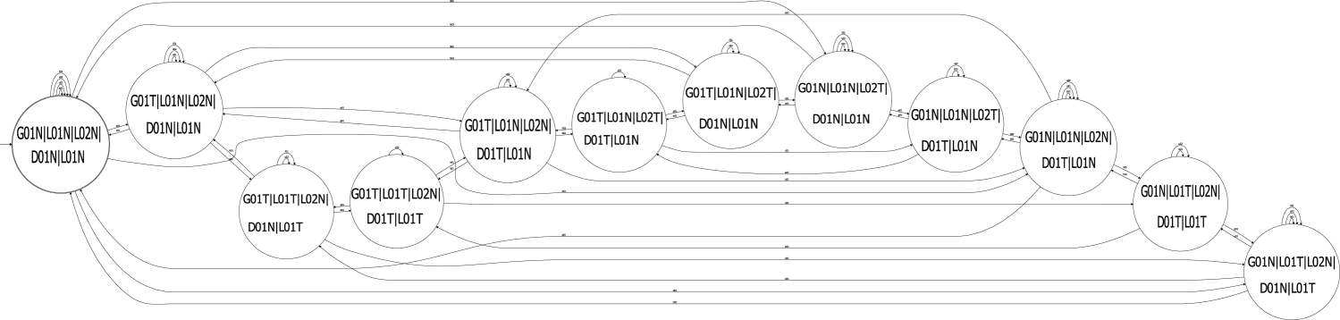
The automaton for node 1 is obtained by parallel composition of components connected to node 1, that is, Generator 1 and Line 1 using libFAUDES software [35].
The resulting automaton is shown in Fig. 5-b.
In the figure, each state is labeled based on the operational state of the component. G01N means the normal state of Generator 1, and G01T means the tripped state of Generator 1.
Similarly, the states of transmission line 1 are labeled as L01N and L01T for the normal and tripped states, respectively.

Using the same method, the automaton for node 2 shown in Fig. 6-b is obtained by parallel composition of components connected to node 2, that is, Load 1, Line 1, and Line 2 shown Fig. 6-a. In the figure, the states for load 1 are denoted by D01N and D01T for the normal and trip states, respectively.
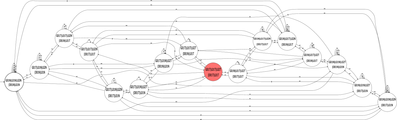
The sub-system model consists of node 1 and its neighboring node, node 2. Hence, is the parallel composition of and :
which is shown in Fig. 7.
V-B Specification
A cascading failure can be defined as a string of uncontrollable events that lead the system from a legal/safe state to some illegal/unsafe states. In this example, the illegal states are
| (113) |
which are marked in red in Fig. 7.
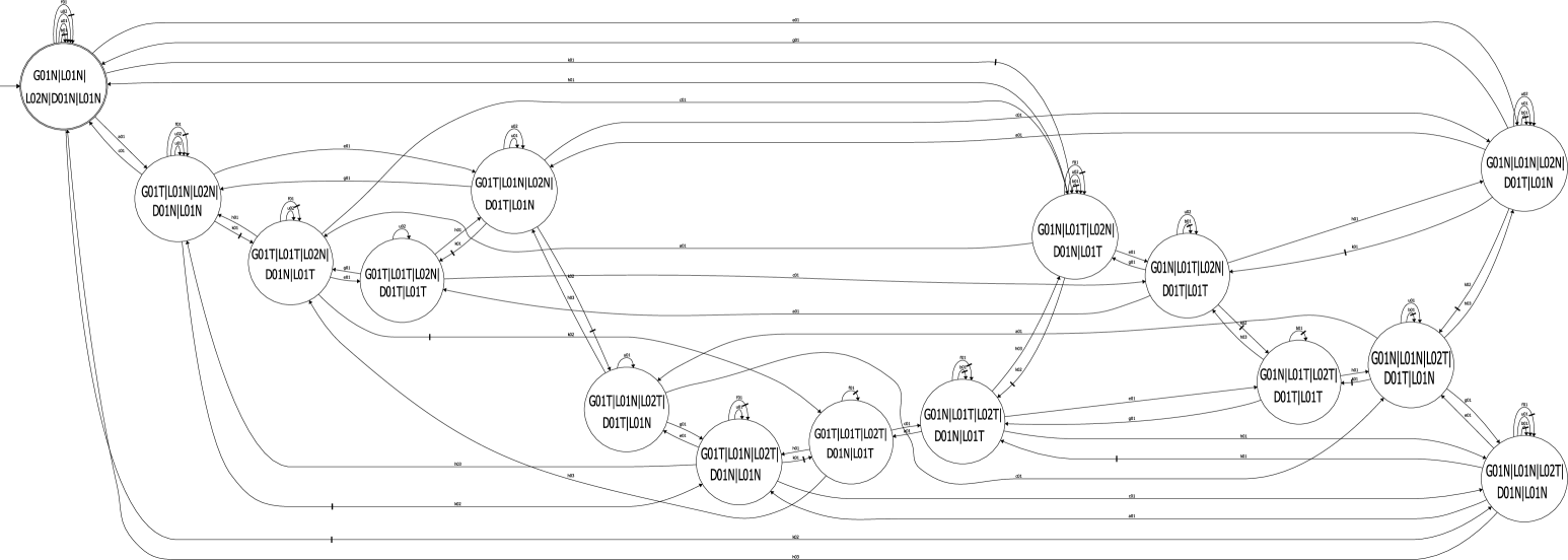
Hence, the sub-automaton generating the specification language is obtained by removing the illegal states from .
is shown in Fig. 8.
V-C Controller synthesis
We use libFAUDES software to synthesize the controllers. In order to synthesize a controller, a plant model and a specification are needed, an the plant model and specification were defined in the previous two subsections. Additionally, controllability attributes need to be defined for events in the system. Table II shows the controllability attributes of the events (whether an event is controllable or forcible). In the modular control framework adopted in this paper, each node or bus in the system has its own plant model, specification, and controller. We only demonstrate the procedure for these processes for node 2 in this illustrative example. The same procedure can be followed for each node for any given power system. Note that transmission lines tripping events are not controllable by themselves, but can be preempted by forcible events. Note also that Load shedding, which is event , and generation re-dispatch, which is event , are both controllable and forcible.
| Component | Component event | Controllable | Forcible |
|---|---|---|---|
| Line | No | No | |
| No | No | ||
| No | No | ||
| Generator | No | No | |
| Yes | Yes | ||
| No | No | ||
| Load | No | No | |
| Yes | Yes | ||
| No | No |
After knowing the controllability attributes and the specification language, a controller can be synthesized for node by applying the method outlined in Section III. Since is F-controllable, . By Equation (92), the controller is given by, for ,
| (117) |
The realization of as an automaton
| (119) |
can be synthesized based on the sub-system model in Fig. 7 and the specification automaton in Fig. 8 using libFAUDES software. The synthesis algorithm is based on [36]. Since libFAUDES is developed for conventional supervisory control without forcible events, we need to modify event attributes as shown in Table II to use libFAUDES. In other words, we view k01 and k02 as controllable, because they can be preempted by b01 and f01. The resulting is shown in Fig. 9. The supervisor synthesis function requires two inputs: The plant automaton with the modified controllability attributes shown in Table II and the specification automaton . Its output is the supervisor automaton or .
| Component | Component event | Controllable | Forcible |
|---|---|---|---|
| Line | No | No | |
| Yes | Yes | ||
| No | No | ||
| Generator | No | No | |
| Yes | Yes | ||
| No | No | ||
| Load | No | No | |
| Yes | Yes | ||
| No | No |
V-D Simulation results
The framework presented above is implemented and simulated for the IEEE 30-bus, 118-bus, and 300-bus systems [38] [39] to verify the findings of the proposed modular control. The single-line diagrams of the IEEE 30-bus, 118-bus and IEEE 300-Bus system are shown in Fig. 10, Fig. 11 and Fig. 12 respectively. It is assumed in this paper that nodes send and receive information to direct neighbors without any time delay. The simulation time, is however, considered and recorded, which includes the computation time of the optimal control actions and the supervisors’ iterators.


The simulation setup is done in MATLAB environment, which is used to simulate the system with Matpower [38] and DCSIMSEP [40, 34]; and to send and receive information from the controllers. The model used in the paper is comparable to the OPA model [41], specifically the fast phase process part, were DC power flow is used and generation redsipatch with LP is implemented. The controllers are implemented in MATLAB, where the DES operations functions are imported from C++ libFAUDES [35] DES library into MATLAB, and as illustrated in Subsections A, B and C. The controllers are synthesized based on the specification and plant models. As mentioned earlier, each node or bus in the power system has its controller; for example, the IEEE 300 bus system has 300 modular controller. To optimally control the amount of load shedding and generation re-dispatch, each of the modular controllers solve the following optimization problem at a given node if the DES controller for that bus allows it.
| (124) |
where are the amounts of load to be shed, is the diagonal matrix of the line admittance, and is the line-node incidence matrix, are the lines max capacities, are the line power flows, is the value of the power transfer distribution factor () of the buses for the critical transmission line , and is the most loaded line in site .
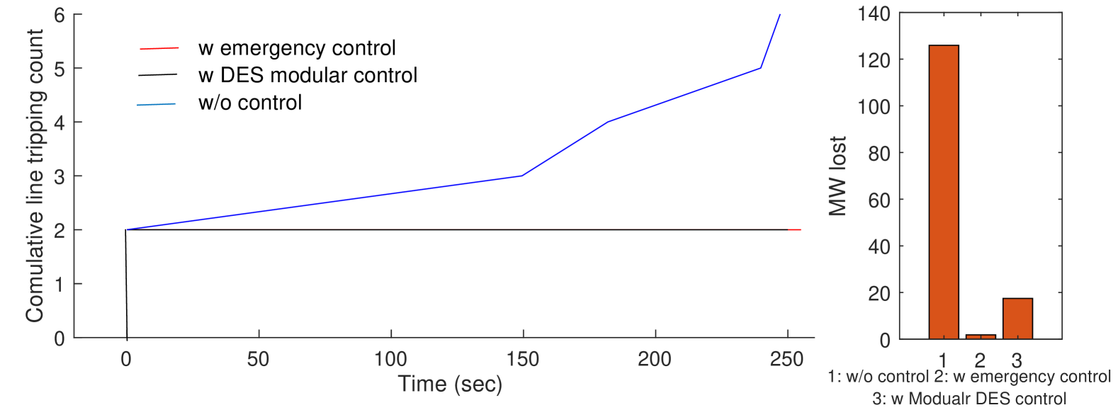
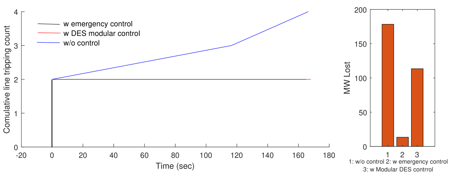
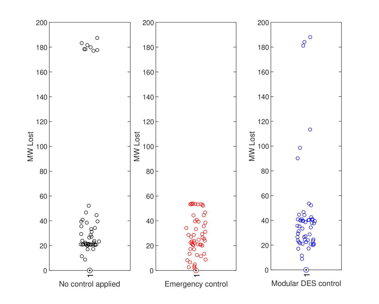
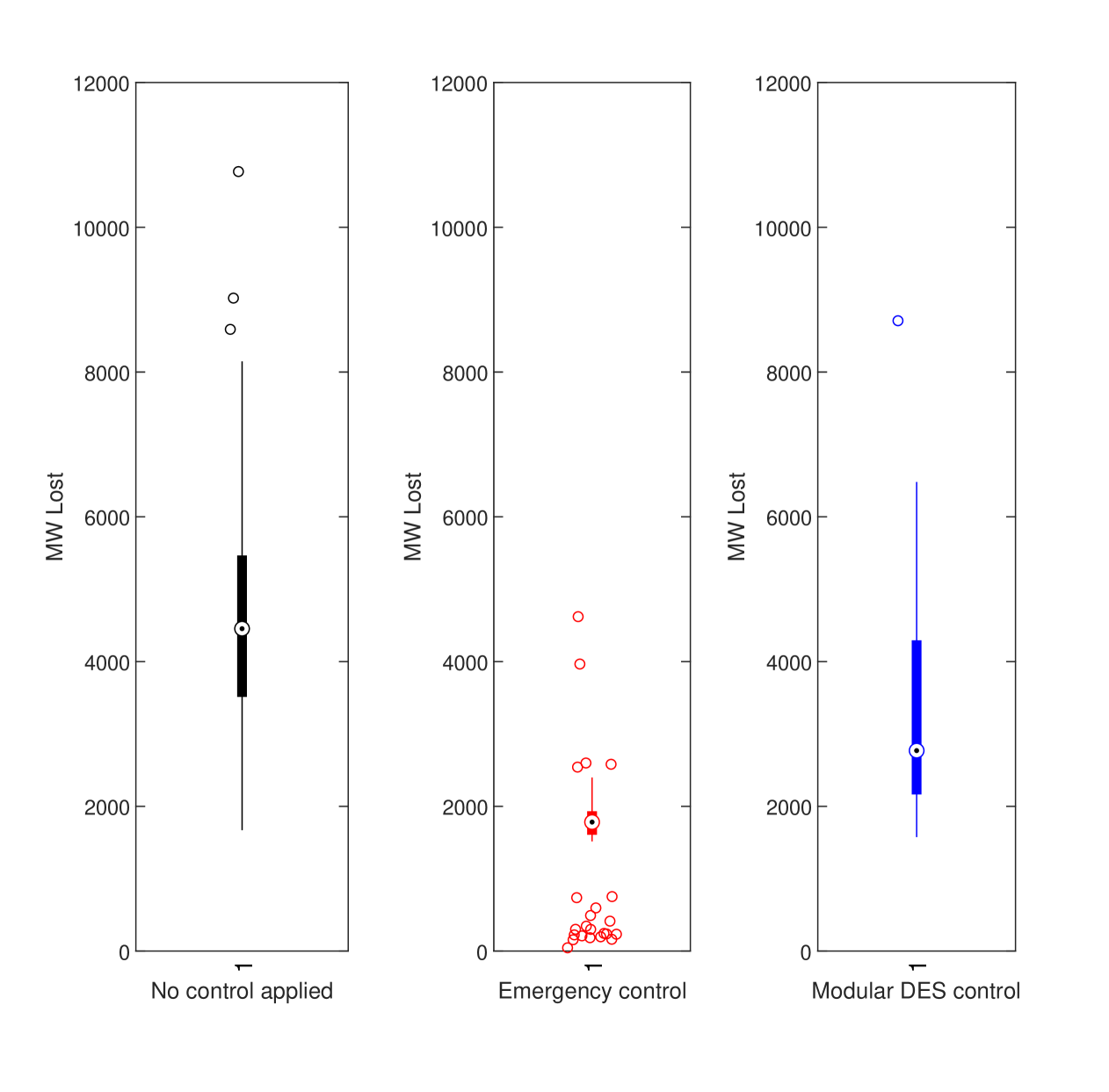
Fig. 13 shows the results of specific scenarios from the IEEE 30-bus system simulation results. The contingency simulated was the lines pair . The modular control approach stopped the failure cascading but with higher MW loss than the LLP DES control method discussed in [25]. The higher MW lost is because, in modular control, the modular supervisors can only make decisions based on the information received from neighboring nodes and send control actions to the neighboring nodes, making the solution local and not global. To further verify our approach, we performed simulation studies on the IEEE-118 bus system. A specific case of the simulation studies is shown in Fig. 14, lines pair were tripped as the initial trip. A typical simulation of the IEEE 300-bus system is shown in Fig. 15, where the contingency of the lines pair is simulated. The proposed modular control stops the failure cascading as desired, but with a higher MW loss than the emergency control method discussed in [42], which is a centralized control method that uses a global optimization for the power system. The higher MW lost is because, in the modular control, the modular controllers can only make decisions based on the information received from neighboring nodes and send control actions to the neighboring nodes, making the solution local and not global. As mentioned in Section III, the modular controller has several advantages over centralized control.

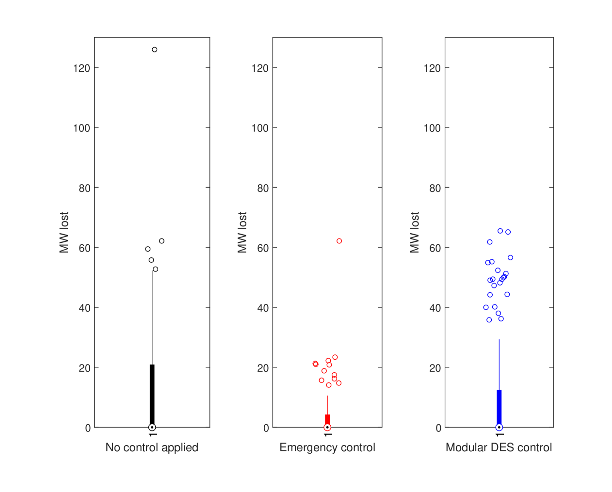
Monte Carlo simulations have been carried out for the three adopted systems to further verify the proposed approach. In the simulations, the initial tripping follows a uniform random distribution.
The loads follow a normal distribution, with a standard deviation of 0.15 per unit from the nominal loads. Results of the simulations and the comparison with the emergency control method and without any control to mitigate the failure cascade are shown in Fig. 16 and Fig. 17 and Fig. 18.
For the IEEE 300 Bus system, the median MW loss for the DES modular control method is 2770 MW. For the emergency control method, it is 1782 MW, and without using any control, it is 4454 MW. Our method shows that it could mitigate the failure cascade in most cases and reduce the overall lost MW in the system.
The results show similar behavior compared to the proposed method in this paper with other methods that are based on modular control [12] [43] [44], while the authors used different indices to express the effectiveness of their proposed approaches. The results, in general, show similar behavior. It is also worth mentioning that in our paper we did not focus on the study of the communication delay between controlling agents on the effectiveness of the proposed approach.
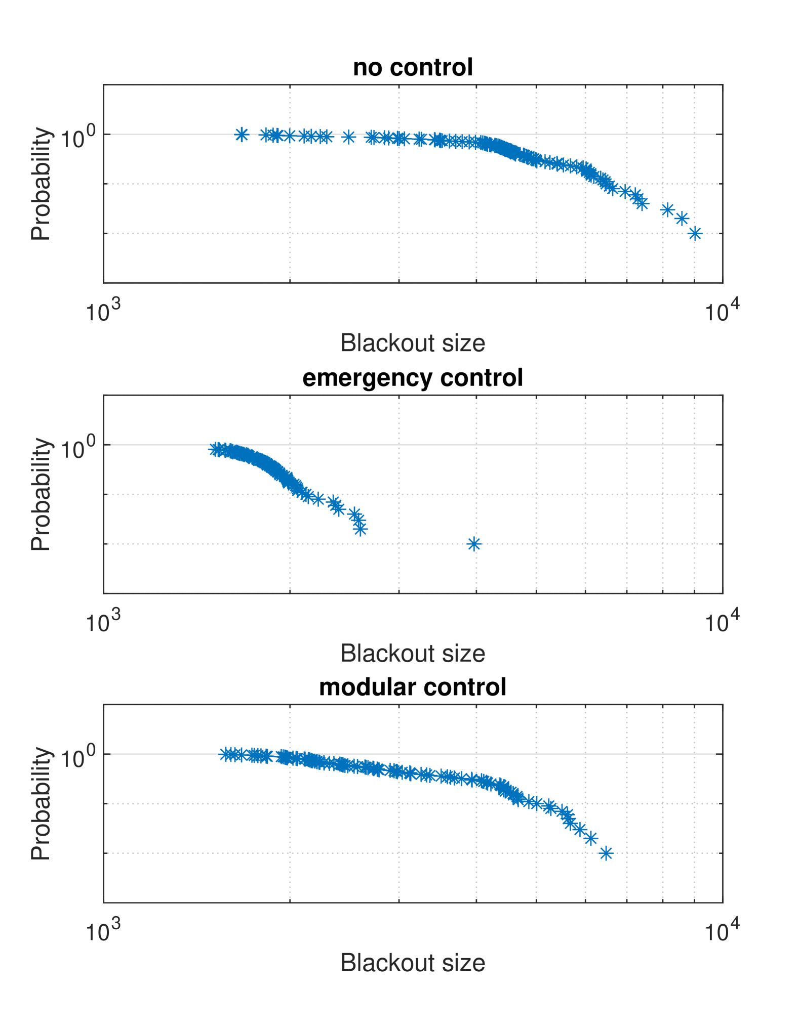
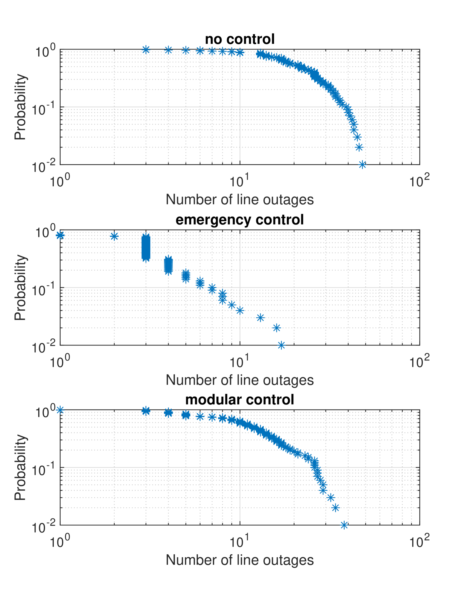
The complementary cumulative distribution (CCD), i.e. log-log plot, of the blackout size in terms of MW lost and its occurrence of the Monte Carlo simulations is shown in Fig. 19, the system without control shows power-law behavior, it also observed from the figure that blackout size reduces when using modular control and reduces even more when emergency control was applied on the system under the same condition, which aligns with our previous analysis. Similarly, Fig. 20 shows a log-log plot of the lines outages probabilities for the IEEE 300-bus system, which also verifies our approach compared to several other approaches adopted in the literature [45].
VI Conclusion
In this paper, we developed a new control to prevent cascading failures in large scale power systems using modular supervisory control of discrete event systems (DES). The modular control reduces computational complexity and increases the effectiveness and robustness of the controlled system. We first extended the modular control approach to include forcible events and expanded the specification language to incorporate more events from neighboring nodes to improve control actions for each modular controller. We proposed a platform based on MATLAB environment to implement the modular strategy that couples the DES and continuous-time parts of the control and tests them with power system simulations. To verify the effectiveness of the proposed approach, we conducted a case study using the IEEE 30-bus, 118-bus and 300-bus systems. The proposed modular supervisory control can successfully stop cascading failures and significantly reduce the MW lost due to the failures. However, compared with the centralized control approach that we proposed in [25], the modular control approach results in more MW lost, and more lines tripped after observing an N-2 contingency. Nevertheless, the modular supervisory control is more reliable since it does not depend on a central controller, and each node only requires information from its neighbors. Our simulation results demonstrate the effectiveness of the proposed approach in mitigating cascading failures in power systems.
References
- [1] P. D. Hines, I. Dobson, and P. Rezaei, “Cascading power outages propagate locally in an influence graph that is not the actual grid topology,” IEEE Transactions on Power Systems, vol. 32, no. 2, pp. 958–967, 2016.
- [2] C. Asavathiratham, S. Roy, B. Lesieutre, and G. Verghese, “The influence model,” IEEE Control Systems Magazine, vol. 21, no. 6, pp. 52–64, 2001.
- [3] K. Zhou, I. Dobson, Z. Wang, A. Roitershtein, and A. P. Ghosh, “A markovian influence graph formed from utility line outage data to mitigate large cascades,” IEEE Transactions on Power Systems, vol. 35, no. 4, pp. 3224–3235, 2020.
- [4] L. Guo, C. Liang, A. Zocca, S. H. Low, and A. Wierman, “Line failure localization of power networks part i: Non-cut outages,” IEEE Transactions on Power Systems, vol. 36, no. 5, pp. 4140–4151, 2021.
- [5] L. Guo, C. Liang, A. Zocca, S. H. Low, and A. Wierman, “Line failure localization of power networks part ii: Cut set outages,” IEEE Transactions on Power Systems, vol. 36, no. 5, pp. 4152–4160, 2021.
- [6] I. B. Sperstad, E. H. Solvang, and S. H. Jakobsen, “A graph-based modelling framework for vulnerability analysis of critical sequences of events in power systems,” International Journal of Electrical Power and Energy Systems, vol. 125, p. 106408, 2021.
- [7] S. Yang, W. Chen, X. Zhang, and W. Yang, “A graph-based method for vulnerability analysis of renewable energy integrated power systems to cascading failures,” Reliability Engineering and System Safety, vol. 207, p. 107354, 2021.
- [8] X. Lian, T. Qian, Z. Li, X. Chen, and W. Tang, “Resilience assessment for power system based on cascading failure graph under disturbances caused by extreme weather events,” International Journal of Electrical Power and Energy Systems, vol. 145, p. 108616, 2023.
- [9] B. Li, D. Ofori-Boateng, Y. R. Gel, and J. Zhang, “A hybrid approach for transmission grid resilience assessment using reliability metrics and power system local network topology,” Sustainable and Resilient Infrastructure, vol. 6, no. 1-2, pp. 26–41, 2021.
- [10] Y. Liu, T. Wang, and J. Guo, “Identification of vulnerable branches considering spatiotemporal characteristics of cascading failure propagation,” Energy Reports, vol. 8, pp. 7908–7916, 2022.
- [11] J. W. Bialek and V. Vahidinasab, “Tree-partitioning as an emergency measure to contain cascading line failures,” IEEE Transactions on Power Systems, vol. 37, no. 1, pp. 467–475, 2022.
- [12] P. Hines and S. Talukdar, “Reciprocally altruistic agents for the mitigation of cascading failures in electrical power networks,” in 2008 First International Conference on Infrastructure Systems and Services: Building Networks for a Brighter Future (INFRA), pp. 1–6, 2008.
- [13] I. A. Perez, D. Ben Porath, C. E. La Rocca, L. A. Braunstein, and S. Havlin, “Critical behavior of cascading failures in overloaded networks,” Phys. Rev. E, vol. 109, p. 034302, Mar 2024.
- [14] R.-R. Liu, C.-X. Jia, M. Li, and F. Meng, “A threshold model of cascading failure on random hypergraphs,” Chaos, Solitons and Fractals, vol. 173, p. 113746, 2023.
- [15] M. Abdelmalak, V. Venkataramanan, and R. Macwan, “A survey of cyber-physical power system modeling methods for future energy systems,” IEEE Access, vol. 10, pp. 99875–99896, 2022.
- [16] X. Bu, W. Yu, L. Cui, Z. Hou, and Z. Chen, “Event-triggered data-driven load frequency control for multiarea power systems,” IEEE Transactions on Industrial Informatics, vol. 18, no. 9, pp. 5982–5991, 2022.
- [17] J. Yang, Q. Zhong, K. Shi, and S. Zhong, “Co-design of observer-based fault detection filter and dynamic event-triggered controller for wind power system under dual alterable dos attacks,” IEEE Transactions on Information Forensics and Security, vol. 17, pp. 1270–1284, 2022.
- [18] S. A. Ghorashi Khalil Abadi and A. Bidram, “A distributed rule-based power management strategy in a photovoltaic/hybrid energy storage based on an active compensation filtering technique,” IET Renewable Power Generation, vol. 15, no. 15, pp. 3688–3703, 2021.
- [19] G. Liu, J. H. Park, C. Hua, and Y. Li, “Hybrid dynamic event-triggered load frequency control for power systems with unreliable transmission networks,” IEEE Transactions on Cybernetics, vol. 53, no. 2, pp. 806–817, 2023.
- [20] M. Abdelmalak and M. Benidris, “Enhancing power system operational resilience against wildfires,” IEEE Transactions on Industry Applications, vol. 58, no. 2, pp. 1611–1621, 2022.
- [21] P. J. Ramadge and W. M. Wonham, “Supervisory control of a class of discrete event processes,” SIAM journal on control and optimization, vol. 25, no. 1, pp. 206–230, 1987.
- [22] F. Lin and W. M. Wonham, “On observability of discrete-event systems,” Information sciences, vol. 44, no. 3, pp. 173–198, 1988.
- [23] W. Wonham, K. Cai, and K. Rudie, “Supervisory control of discrete-event systems: A brief history,” Annual Reviews in Control, vol. 45, pp. 250–256, 2018.
- [24] W. H. Al-Rousan, C. Wang, and F. Lin, “A discrete event theory based approach for modeling power system cascading failures,” in 2019 IEEE Power Energy Society General Meeting (PESGM), pp. 1–5, 2019.
- [25] W. Al-Rousan, C. Wang, and F. Lin, “A discrete-event system approach for modeling and mitigating power system cascading failures,” IEEE Transactions on Control Systems Technology, vol. 30, no. 6, pp. 2547–2560, 2022.
- [26] W. A. Rousan, Power Systems Cascading Failure Analysis And Mitigation Using Discrete Events Systems Approach. PhD thesis, Wayne State University, 2022.
- [27] W. M. Wonham and P. J. Ramadge, “Modular supervisory control of discrete-event systems,” Mathematics of control, signals and systems, vol. 1, no. 1, pp. 13–30, 1988.
- [28] K. C. Wong and W. M. Wonham, “Modular control and coordination of discrete-event systems,” Discrete Event Dynamic Systems, vol. 8, pp. 247–297, 1998.
- [29] J. Komenda and J. H. van Schuppen, “Control of discrete-event systems with modular or distributed structure,” Theoretical Computer Science, vol. 388, no. 1-3, pp. 199–226, 2007.
- [30] C. Zhou, R. Kumar, and R. S. Sreenivas, “Decentralized modular control of concurrent discrete event systems,” in 2007 46th IEEE Conference on Decision and Control, pp. 5918–5923, IEEE, 2007.
- [31] N. D. Kouvakas, F. N. Koumboulis, D. G. Fragkoulis, and A. Souliotis, “Modular supervisory control for the coordination of a manufacturing cell with observable faults,” Sensors, vol. 23, no. 1, 2023.
- [32] C. Pasquale, S. Sacone, S. Siri, and A. Ferrara, “Hierarchical centralized/decentralized event-triggered control of multiclass traffic networks,” IEEE Transactions on Control Systems Technology, vol. 29, no. 4, pp. 1549–1564, 2021.
- [33] A. Karimoddini, M. Karimadini, and H. Lin, “Decentralized modular hybrid supervisory control for the formation of unmanned helicopters,” IET Control Theory and Applications, vol. 17, no. 2, pp. 210–222, 2023.
- [34] P. Rezaei, P. D. H. Hines, and M. J. Eppstein, “Estimating cascading failure risk with random chemistry,” IEEE Transactions on Power Systems, vol. 30, no. 5, pp. 2726–2735, 2015.
- [35] T. Moor, K. Schmidt, and S. Perk, “libfaudes — an open source c++ library for discrete event systems,” in 2008 9th International Workshop on Discrete Event Systems, pp. 125–130, 2008.
- [36] C. G. Cassandras and S. Lafortune, Introduction to discrete event systems. Springer Science & Business Media, 2009.
- [37] J. Komenda, T. Masopust, and J. H. van Schuppen, “On conditional decomposability,” Systems & Control Letters, vol. 61, no. 12, pp. 1260–1268, 2012.
- [38] R. D. Zimmerman, C. E. Murillo-Sánchez, and R. J. Thomas, “Matpower: Steady-state operations, planning, and analysis tools for power systems research and education,” IEEE Transactions on Power Systems, vol. 26, no. 1, pp. 12–19, 2011.
- [39] “Power systems test case archive.” http://labs.ece.uw.edu/pstca/pf300/pg_tca300bus.htm. Accessed: 2024-04-17.
- [40] M. J. Eppstein and P. D. H. Hines, “A “random chemistry” algorithm for identifying collections of multiple contingencies that initiate cascading failure,” IEEE Transactions on Power Systems, vol. 27, no. 3, 2012.
- [41] B. A. Carreras, V. E. Lynch, I. Dobson, and D. E. Newman, “Complex dynamics of blackouts in power transmission systems,” Chaos: An Interdisciplinary Journal of Nonlinear Science, vol. 14, pp. 643–652, 09 2004.
- [42] R. Pooya, Cascading Failure Risk Estimation and Mitigation in Power Systems. PhD thesis, University of Vermont, 2016.
- [43] B. Shi and J. Liu, “Decentralized control and fair load-shedding compensations to prevent cascading failures in a smart grid,” International Journal of Electrical Power and Energy Systems, vol. 67, pp. 582–590, 2015.
- [44] M. Warnier, S. Dulman, Y. Koç, and E. Pauwels, “Distributed monitoring for the prevention of cascading failures in operational power grids,” International Journal of Critical Infrastructure Protection, vol. 17, pp. 15–27, 2017.
- [45] K. Sun, Cascading Failures in Power Grids: Risk Assessment, Modeling, and Simulation. Springer International Publishing AG, 2024.