Echoes of Disagreement: Measuring Disparity in Social Consensus

Abstract

Public discourse and opinions stem from multiple social groups. Each group has its own beliefs about a topic (such as vaccination, abortion, gay marriage, etc.), and opinions are exchanged and blended to produce consensus. A particular measure of interest corresponds to measuring the influence of each group on the consensus and the disparity between groups on the extent they influence the consensus. In this paper, we study and give provable algorithms for optimizing the disparity under the DeGroot or the Friedkin-Johnsen models of opinion dynamics. Our findings provide simple poly-time algorithms to optimize disparity for most cases, fully characterize the instances that optimize disparity, and show how simple interventions such as contracting vertices or adding links affect disparity. Finally, we test our developed algorithms in a variety of real-world datasets.

1 Introduction

Public discourse and opinions emerge from diverse social groups, each holding distinct beliefs on topics like vaccination, abortion, and gay marriage. Through the exchange and blending of these opinions, a consensus is formed. This dynamic exchange is essential for societal decision-making and policy development. As people engage in discussions, their views are shaped by their communities’ collective attitudes and experiences. These interactions, enabled by various social, political, and media channels, drive the evolution of public sentiment. Understanding how these exchanges take place and how consensus is reached is vital for understanding the mechanisms of social influence and the resilience of networked systems amid differing opinions.

Measuring how the intrinsic opinions of different groups affect the consensus is an important task. Namely, given two groups $A$ and $B$, each with some intrinsic opinions, what can one say about the consensus due to the opinions stemming only from $A$ and the consensus due to the opinions stemming only from $B$? Our work is set to study this problem. Namely, we introduce the disparity measure, which corresponds to the difference between consensus values if only the opinions in group $A$ are taken into account and the consensus values if only the opinions in group $B$ are taken into account. The disparity measure is related to notions regarding measuring and optimizing network statistics such as polarization and disagreement (Musco et al., 2018; Gionis et al., 2013; Chen and Rácz, 2021; Gaitonde et al., 2021; Racz and Rigobon, 2022).

We study the disparity measure under two well-known opinion dynamics models: the DeGroot model (DeGroot, 1974) and the Friedkin-Johnsen model (Friedkin and Johnsen, 1990), and provide algorithms to maximize (resp. minimize) the disparity metric. We demonstrate that for the DeGroot model, minimizing the disparity about either the topology or the initial opinions can be achieved with a polynomial-time algorithm. However, finding the partition that minimizes disparity is an NP-hard problem. Furthermore, we show that maximizing the disparity measure under the DeGroot model can be solved in polynomial time to determine the optimal topology and partition subject to cardinality constraints. For the FJ model, we establish that the minimum disparity is independent of the graph topology and corresponds to a trivial graph partitioning.

Additionally, the disparity for the FJ model is maximized when the graph is a complete bipartite graph. We then study two common topologies based on the stochastic block model (two cliques and core-periphery) and study the effect of assortativity on the minimum disparity. Finally, we show how we can provably reduce disparity in the FJ model by changing the weight of links and test our method on real-world datasets.

2 Setup and Models

Notation.

$\mathbf{1}$ refers to the vector of all ones, and $\bar{\mathbf{1}}$ refers to the normalized vector of all ones (i.e., with entries $1/\sqrt{n}$. $a\odot b$ denotes element-wise multiplication between vectors $a,b$. $i\sim j$ denotes a (directed) edge from $i$ to $j$. $|v|$ denotes the element-wise absolute value of vector $v$.

Network.

We assume a weighted connected network $G(V,E)$ on $|V|=n$ nodes. Each edge $(i,j)\in E$ is associated with a non-negative cost $w:E\to\mathbb{R}_{\geq 0}$. Suppose that the corresponding adjacency matrix is $W$ has entries $w_{ij}>0$ for each edge $(u,v)\in E$ and zero elsewhere, and the weighted-degree matrix $D$ has diagonal entries $d_{i}=\sum_{(j,i)\in E}w_{ij}$. We define $m=\frac{1}{2}\sum_{(i,j)\in E}w_{ij}$. If $G$ is undirected, the Laplacian $L=D-W$ of $G$ has eigenvalues $\lambda_{n}(G)\geq\lambda_{n-1}(G)\geq\dots\geq\lambda_{1}(G)=0$, where the zero eigenvalue corresponds to the eigenvector $v_{1}=\bar{\mathbf{1}}$.

Each agent $i\in V$ has an intrinsic opinion $s_{i}\in[0,1]$ corresponding to her internal belief about a topic. Throughout the paper, we assume that the intrinsic belief vector is normalized, namely $\|s\|=1$.

DeGroot Model.

The DeGroot model (DeGroot, 1974) is based on a simpler principle than the FJ model. For the DeGroot updates, we assume that $G$ is directed. According to the DeGroot model, every agent updates her opinions according to the following:

$$x_{i}(t+1)=\sum_{i\sim j}T_{ij}x_{j}(t),$$ (1)

where initially we have $x_{i}(0)=s_{i}$ and $T_{ij}$ are the mixing weights which correspond to a row stochastic transition matrix $T$ with entries $T_{ij}\geq 0$ if $(i,j)\in E$ and $T_{ij}=0$ for $(i,j)\notin E$ (e.g., $T_{ij}=w_{ij}/\sum_{i\sim k}w_{ik}$). It is easy to show that the consensus (or equilibrium) $z=\lim_{t\to\infty}x(t)$ subject to (1) satisfies

$$z=(q^{\top}s)\mathbf{1},$$ (2)

where $q$ is the principal eigenvector of $T$.

Friedkin-Johnsen Model.

In the Friedkin-Johnsen model (Friedkin and Johnsen, 1990) (FJ), each agent suffers a quadratic cost for not reaching a consensus with respect to her neighbors and her intrinsic opinion (Bindel et al., 2015). This yields the following update rule for each agent $i$:

$$x_{i}(t)=\sum_{i\sim j}T_{ij}x_{j}(t)+T_{ii}s_{i},$$ (3)

where the weights $T_{ij}$ are set as $T_{ij}=\frac{w_{ij}}{\sum_{j\sim k}w_{ik}+w_{ii}}$. It is also known that (3) converges to a fixed point $z=\lim_{t\to\infty}x(t)$, that equals:

$$z=(I+L)^{-1}s.$$ (4)

For the FJ model we assume that $G$ is undirected.

3 Measuring Disparity

Let the vertex set $V$ be partitioned into two sets $A$ and $B=V\setminus A$ and let $s_{A}$ (resp. $s_{B}$) be the vector of intrinsic opinions due to set $A$, namely

$$s_{A,i}=\begin{cases}s_{i},&i\in A\\ 0,&i\in B\end{cases},$$

where the vector $s_{B}$ is defined similarly. The consensus due to $s_{A}$ is denoted as $z_{A}$ and the consensus due to $s_{B}$ is denoted as $z_{B}$. We define the disparity as the difference of the contribution between groups $A$ and $B$ to the consensus $z$:

$$f(s,A,T)=\|z_{A}-z_{B}\|^{2}.$$ (5)

We have omitted $B$ as an argument since we assume always that $B=V\setminus A$, i.e., the partition is always characterized by $A$. The sentiment strength of $A$ (resp. $B$) is defined as

$$S_{A}=\mathbf{1}^{\top}s_{A},\;S_{B}=\mathbf{1}^{\top}s_{B}$$

and the sentiment imbalance is defined to be

$$\kappa_{AB}=\max\left\{\frac{S_{A}}{S_{B}},\frac{S_{B}}{S_{A}}\right\}.$$

For the DeGroot model, the disparity equals

$$f^{\mathsf{DG}}(s,A,T)=n(q^{\top}(s_{A}-s_{B}))^{2}.$$ (6)

According to the FJ model, the disparity equals

$$f^{\mathsf{FJ}}(s,A,T)=(s_{A}-s_{B})^{\top}(I+L)^{-2}(s_{A}-s_{B}).$$ (7)

4 Disparity in the DeGroot Model

4.1 Disparity Minimization

It is straigthforward to see that disparity is minimized, and has zero objective value, when $q^{\top}(s_{A}-s_{B})=0$, that is $s_{A}$ and $s_{B}$ have equal projections onto $q$.

Finding $s$.

Intrinsic opinions represent the starting points of users’ perspectives before interactions on the platform. From a platform perspective, strategically shaping or influencing these intrinsic opinions – through design, education, or content curation – can help minimize disparities between the consensus values of different groups.

Technically, we want to solve

$$s^{*}=\operatorname*{arg\,min}_{s:\|s\|=1}f^{\mathsf{DG}}(s,A,T).$$

Therefore, if we know the DeGroot weights and the partition $(A,B)$ and we want to construct the internal opinion vectors, we can find $s^{*}$ (in general, the problem has an infinite amount of solutions; here we provide one that is efficiently computable and interpretable) as follows: We assume that $s^{*}$ has a constant value $\alpha$ in $A$ and a constant value $\beta$ in $B$. The projection requirement and the normalization constraint for the norm of $s^{*}$ give the following system of equations:

$$\alpha^{2}|A|+\beta^{2}|B| =1,$$

$$\alpha Q_{A}-\beta Q_{B} =0,$$

where $Q_{A}=\sum_{i\in A}q_{i}$ and $Q_{B}=\sum_{i\in B}q_{i}$. Solving the system, we get

$$s_{i}^{*}=\begin{cases}\sqrt{\frac{1}{|A|+(Q_{A}/Q_{B})^{2}|B|}},&i\in A,\\ \sqrt{\frac{1}{|A|(Q_{B}/Q_{A})^{2}+|B|}},&i\in B\end{cases}.$$ (8)

An interesting and simple case to study the behavior of the intrinsic opinion vector is on a Markov chain where the principal eigenvector corresponds to the uniform distribution, i.e., $q_{i}=1/n$. In that case, Eq. 8 becomes

$$s_{i}^{*}=\begin{cases}\sqrt{\frac{|B|}{n|A|}},&i\in A,\\ \sqrt{\frac{|A|}{n|B|}},&i\in B\end{cases}$$

Finding $G$.

In many social networks, the structure $G$ of connections – who interacts with whom – plays a crucial role in shaping consensus outcomes. These connections determine how opinions flow and influence one another, often amplifying disparities when the network is segregated or highly imbalanced. By strategically optimizing the social network structure, it becomes possible to reduce the disparity in consensus values and foster more equitable outcomes, even when intrinsic opinions and group memberships differ. Thus, to find $G$ knowing the opinion vector $s$ and the partition $(A,B)$, we seek

$$T^{*}=\operatorname*{arg\,min}_{T:T\mathbf{1}=\mathbf{1},T\geq\mathbf{0},\mathrm{supp}(T)=G}f^{\mathsf{DG}}(s,A,T).$$

We can construct $q^{*}$ to have entries $q_{i}^{*}$ as follows: We assume that $q$ has a constant value $\alpha^{\prime}$ in $A$ and a constant value $\beta^{\prime}$ in $B$. The projection requirement and the simplex constraint give the following system of equations:

$$\alpha^{\prime}|A|+\beta^{\prime}|B| =1,$$

$$\alpha^{\prime}S_{A}-\beta^{\prime}S_{B} =0,$$

Solving the system yields:

$$q_{i}^{*}=\begin{cases}\frac{1}{|A|+(S_{A}/S_{B})|B|},&i\in A\\ \frac{1}{|A|(S_{B}/S_{A})+|B|},&i\in B\end{cases}.$$ (9)

When $s=\bar{\mathbf{1}}$, (9) becomes

$$q_{i}^{*}=\begin{cases}\frac{1}{2|A|},&i\in A,\\ \frac{1}{2|B|},&i\in B\end{cases}.$$

Constructing the Markov Chain. For a general value of $s$, we can construct the DeGroot weights such that the stationary distribution is $q^{*}$. One natural choice is the Metropolis-Hastings weights, which allow us to set up a Markov chain with the desired stationary distribution of $q^{*}$ (Boyd et al., 2004). According to the Metropolis-Hastings weights, a regulator can set the learning weights as follows:

$$T_{ij}^{*}=\begin{cases}\frac{1}{\max\{d_{i},d_{j}\}},&i,j\in A\text{ or }i,j\in B,\\ \frac{1}{\max\{d_{i},(S_{B}/S_{A})d_{j}\}}&i\in A,j\in B\\ \frac{1}{\max\{d_{i},(S_{A}/S_{B})d_{j}\}}&i\in B,j\in A\end{cases}.$$ (10)

for $i\sim j$, and $T_{ii}^{*}=1-\sum_{i\sim j}T_{ij}^{*}$. Alternatively, one can construct the Markov chain to have $q^{*}$ as its stationary distribution subject to minimizing its mixing time by solving a convex optimization problem (Boyd et al., 2004). Figure 1 shows the weights of the disparity-minimizing Markov Chain on the Karate Club network, where the partitions are taken according to the spectral clustering of the network.

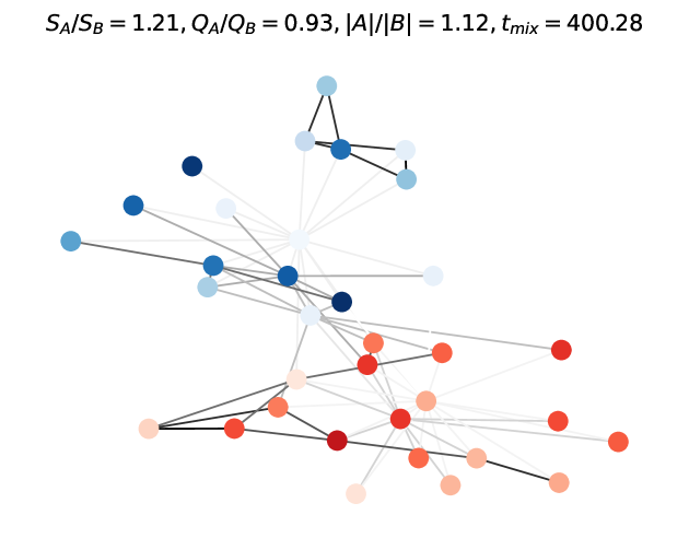
(a) Non-polarized Network

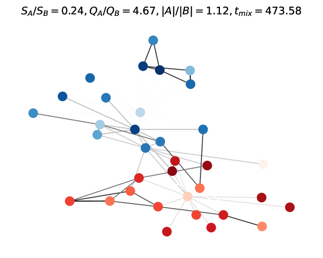
(b) Polarized Network

Figure 1: Disparity Minimizing Markov Chain weights for the Karate Club Network. The node labels in (a) correspond to the intrinsic opinions of the nodes where $s=s^{\prime}/\|s^{\prime}\|$ with $s^{\prime}\sim\mathcal{U}\left([0,1]^{n}\right)$. The edge colors correspond to the values of $T_{ij}$. The node labels in (b) correspond to a polarized network where each node in partition $A$ has an intrinsic opinion $s_{i}\sim\mathrm{Beta}(2,8)$ and each node in partition $B$ has an intrinsic opinion $s_{i}\sim\mathrm{Beta}(8,2)$. The node colors correspond to how far each node is from the average opinion. We observe that the high-value weights in the non-polarized network are amplified in the polarized network, and the low-value weights are de-amplified. Moreover, the Markov Chain defined according to the polarized network mixes slower than the non-polarized one.

Bias Amplification due to Sentiment Strength.

If the underlying proposal network is $d$-regular, then Eq. 10 corresponds to

$$T_{ij}^{*}=\begin{cases}\frac{1}{d},&i,j\in A\text{ or }i,j\in B,\\ \frac{1}{d\max\{1,(S_{B}/S_{A})\}}&i\in A,j\in B,\\ \frac{1}{d\max\{1,(S_{A}/S_{B})\}}&i\in B,j\in A,\end{cases}$$ (11)

for all edges $(i,j)\in E$ yielding the following interesting phenomenon: If $S_{A}\geq S_{B}$, then the transition probability from $B$ to $A$ or from $B$ to itself is smaller than the transition probability from $A$ to $B$, which is amplified by a factor (bias) of $S_{A}/S_{B}$. Similarly, when $S_{B}\geq S_{A}$, then the transition probability from $B$ to $A$ is amplified by a factor of $S_{B}/S_{A}$. The bias is eliminated whenever $S_{A}=S_{B}$.

Finding the Partition.

A critical challenge arises when user groups with differing intrinsic opinions converge to form a consensus, potentially leading to disparities that reflect systemic biases or unequal influence. Identifying groups that naturally minimize these disparities allows platforms to design interventions and promote interactions that encourage the formation of communities where the disparity is small.

On a technical note, finding the best partition that minimizes disparity is an NP-Hard problem. given a graph $G$ and an initial vector $s$. The optimization problem is

$$A^{*}=\operatorname*{arg\,min}_{A\subseteq V}f^{\mathsf{DG}}(s,A,T),$$

with the corresponding decision version:

Given a network $G$ with $n$ nodes, a vector $s\in[0,1]^{n}$ of intrinsic opinions, and a target $D$, does there exist a partition of the network $G$ to groups $A$ and $B=V\setminus A$ such that running the DeGroot model produces a disparity equal to $D$?

We call this problem $(2,D)$-DeGroot-Disparity. We prove that solving $(2,D)$-DeGroot-Disparity is as hard as solving a $(2,t)$-Partition problem. The $(2,t)$-Abs-Partition problem is NP-Hard states that:

Given element set $X=\{x_{1},\dots,x_{m}\}$ and a target $t$ does there exist a partition of $X$ into $S$ and $\bar{S}=S\setminus A$ such that $\left|\sum_{i\in S}x_{i}-\sum_{i\in\bar{S}}x_{i}\right|=t$?

Theorem 1.

The $(2,D)$-DeGroot-Disparity problem is NP-Hard.

The above problem is a weakly NP-Hard problem. For instance, in practice, we can leverage the FPTAS algorithm from Kellerer et al. (2003) to solve it or other methods used for subset sum problems, such as the randomized rounding algorithm.

4.2 Disparity Maximization

In the opposite direction than minimization, we explore constructions that maximize disparity. In the previous section, we proved that finding the structure and the intrinsic opinion vector that minimize disparity are problems that admit poly-time algorithms; however, finding the partition that minimizes the disparity is an NP-Hard problem. Certainly, platforms need to avoid high disparity values among their groups. High disparity can be created through various ways: link recommendation algorithms – see also the filter-bubble theory introduced in Pariser (2011) –, strategic actors, and pre-existing polarized groups. It is thus worthwhile to explore under which regimes the disparity is maximized. In the sequel, we give results on maximizing disparity in the DeGroot model:

Finding $G$.

On the maximization problem, it is straightforward that given the intrinsic opinions $s$ and the partition $(A,B)$, the graph that maximizes disparity corresponds to the graph with principal eigenvector $q^{*}$ such that $q_{i^{*}}^{*}=1$ and $q_{i}^{*}=0$ for any $i^{*}\neq i$ where $i^{*}=\mathrm{argmax}_{i\in V}s_{i}$. In that case, the network corresponds to the trivial 1-node network, and the disparity equals $1$.

Finding $s$.

Similarly, the opinion vector that maximizes the disparity is such that $s_{i^{*}}^{*}=1$ and $s_{i}^{*}=0$ for any $i^{*}\neq i$ where $i^{*}=\mathrm{argmax}_{i\in V}q_{i}$. In that case, the value of the disparity equals $nq_{i^{*}}^{2}$.

Finding $A$.

To find the partition and the initial vector that maximizes disparity, we first observe that it is straightforward that taking $A=V^{*},B=\emptyset$ maximizes the disparity and makes it equal to $n(q^{\top}s)^{2}$. However, if the partitions have cardinality constraints, the problem becomes mathematically interesting. Therefore, the optimization problem we are interested in is

$$A^{*}=\operatorname*{arg\,max}_{A\subseteq V:|A|=k}f^{\mathsf{DG}}(s,A,T).$$

To solve this problem, the algorithm is straightforward and is based on the rearrangement inequality. The rearrangement inequality states that given two sorted sequences $\alpha_{1}\leq\alpha_{2}\leq\dots\leq\alpha_{n}$ and $\beta_{1}\leq\beta_{2}\leq\dots\leq\beta_{n}$ of real numbers and permutation $\pi:[n]^{*}\to[n]^{*}$ we have that

$$\sum_{i=1}^{n}\alpha_{n-i+1}\beta_{i}\leq\sum_{i=1}^{n}\alpha_{\pi(i)}\beta_{i}\leq\sum_{i=1}^{n}\alpha_{i}\beta_{i}$$

Theorem 2.

There is an algorithm that solves $\max_{A\subseteq V:|A|=k}n(q^{\top}(s_{A}-s_{B}))^{2}$ in $O(n\log n)$ time.

Finally, if we want to jointly maximize the disparity over $G,s$ and $A$, then it suffices, due to the Cauchy-Schwartz inequality, to take $A=V$, $q$ to be colinear with $s_{A}-s_{B}=s$, and $s$ is a point mass vector, yielding a disparity value of $n$.

Theorem 3.

In the DeGroot model, both finding the topology $G$ that maximizes disparity and finding the partition $(A,B)$ that maximizes disparity subject to $|A|=k$ admit poly-time algorithms.

5 Friedkin-Johnsen Model

We remind the reader that for the FJ model, the disparity equals

$$f^{\mathsf{FJ}}(s,A,T)=(s_{A}-s_{B})^{\top}(I+L)^{-2}(s_{A}-s_{B}),$$

Note that $(I+L)^{-2}$ is simultaneously diagonalizable and that if $\mu_{n}(G)\geq\mu_{n-1}(G),\dots\geq\mu_{1}(G)$ are the eigenvalues of $(I+L)^{-2}$ we have that

$$\mu_{i}(G)=\frac{1}{(1+\lambda_{n-i}(G))^{2}}.$$

5.1 Disparity Minimization

Globally Optimal Structure.

The first problem we are interested in is finding the globally optimal structure that minimizes disparity, i.e., solve

$$(s^{*},A^{*},T^{*})=\operatorname*{arg\,min}_{s,A,T:s\in[0,1]^{n},\|s\|=1,T\geq\mathbf{0},T\mathbf{1}=\mathbf{1}}f^{\mathsf{FJ}}(s,A,T).$$

The disparity is minimized when $s_{A}^{*}-s_{B}^{*}$ corresponds to the eigenvector of $(I+L)^{-2}$ with the minimum eigenvalue $\mu_{1}=\frac{1}{(1+\lambda_{n}(G))^{2}}$. We know that for any $d$-regular graph, the maximum value of the maximum eigenvalue is achieved whenever $G$ is bipartite and is equal to $2d$. Let $L$ and $R$ be the two sets of the bipartite graph, then the eigenvector $v_{n}$ with $v_{n,i}=1/\sqrt{n}$ iff $i\in L$ and $v_{n,i}=-1/\sqrt{n}$ iff $i\in R$ corresponds to $\lambda_{n}(G)=2d$. Regarding the allocation, we want $s_{A}^{*}-s_{B}^{*}=v_{n}$. This can be achieved if and only if $A^{*}=L$, and $s^{*}=|v_{n}|$. Moreover, letting $d=n/2$ – i.e. $G$ is the complete bipartite graph $K_{n/2,n/2}$, the largest eigenvalue is maximized and equals $n$. Thus, the minimum value of the disparity objective becomes $\left(\frac{1}{n+1}\right)^{2}>0$. Contrary to the DeGroot model, where a value of 0 for the disparity can be achieved, the FJ model has a lower bound on the disparity (for any $G,s,A$) bounded away from 0.

Finding $s$ and $A$.

The second problem we are interested in is

$$(s^{*},A^{*})=\operatorname*{arg\,min}_{s,A,:s\in[0,1]^{n},\|s\|=1}f^{\mathsf{FJ}}(s,A,T).$$

It is straightforward (see also (Gaitonde et al., 2021)) that $s_{A}^{*}-s_{B}^{*}=v_{n}$ which yields $A^{*}=\{i\in V:v_{n,i}\geq 0\}$ and $s^{*}=|v_{n}|$, yielding a disparity value of $1/(1+\lambda_{n}(G))^{2}$.

Finding $G$.

Another problem related to the problem of minimizing polarization in opinion dynamics (Musco et al., 2018) is the one of finding the graph that minimizes disparity given a vector of opinions and a partition, i.e.

$$T^{*}=\operatorname*{arg\,min}_{T:T\geq 0,T\mathbf{1}=\mathbf{1}}f^{\mathsf{FJ}}(s,A,T),$$

which is equivalent to

$$L^{*}=\operatorname*{arg\,min}_{L\in\mathcal{L},\mathrm{tr}(L)=2m}(s_{A}-s_{B})^{\top}(I+L)^{-2}(s_{A}-s_{B}),$$

where $\mathcal{L}$ is the space of all Laplacians of connected undirected graphs with trace equal to $2m$, whose row normalization would yield $T^{*}$. It is known (see (Musco et al., 2018; Boyd and Vandenberghe, 2004)) that $x^{\top}(I+L)^{-2}x$ is matrix-convex in $L$. In the appendix, we show that for an edge $e$, the derivative with respect to $w_{e}$ equals

$$\frac{\partial f^{\mathsf{FJ}}}{\partial w_{e}}=-(s_{A}-s_{B})^{\top}X\left[Xb_{e}b_{e}^{\top}+b_{e}b_{e}^{\top}X\right]X(s_{A}-s_{B}),$$

where $X=(I+L)^{-1}$, and $b_{e}$ is the edge’s incidence vector. Therefore, we can run stochastic gradient descent and normalize the weights such that the trace is $2m$ and $T$ has a row-sum of 1. We can furthermore show, as a direct consequence of Musco et al. (2018, Theorem 3) that there is a graph with $O(n\log n/\varepsilon^{2})$ edges that approximates the disparity within an $(1+2\varepsilon)$-factor, by applying Spielman and Srivastava (2008):

Corollary 4.

There exists a network $T^{\mathsf{SOL}}$ with $O(n\log n/\varepsilon^{2})$ edges such that

$$f^{\mathsf{FJ}}(s,A,T^{\mathsf{SOL}})\leq\left(1+2\varepsilon+O(\varepsilon^{2})\right)f^{\mathsf{FJ}}(s,A,T^{\mathsf{OPT}}),$$

where $T^{\mathsf{OPT}}$ is the network that minimizes the disparity.

5.2 Disparity Maximization

Globally Optimal Structure.

Similar to the minimization case, the first problem we are interested at is finding the globally optimal structure that maximizes disparity, i.e., solve

$$(s^{*},A^{*},T^{*})=\operatorname*{arg\,max}_{s,A,T:s\in[0,1]^{n},\|s\|=1,T\geq\mathbf{0},T\mathbf{1}=\mathbf{1}}f^{\mathsf{FJ}}(s,A,T).$$

The disparity is maximized when $s_{A}-s_{B}$ corresponds to the eigenvector of $(I+L)^{-2}$ with the maximum eigenvalue $\mu_{n}(G)=1$, which yields $s_{A}^{*}-s_{B}^{*}=\bar{\mathbf{1}}$, since $\lambda_{1}(G)=0$ for any graph $G$. The relation $s_{A}^{*}-s_{B}^{*}=\bar{\mathbf{1}}$ implies that optimal partition corresponds to $A^{*}=V$ and $s^{*}=\bar{\mathbf{1}}$. This implies that the maximum disparity equals $1$.

Disparity Maximization Subject to Balanced Sentiment.

Moreover, if we want to find the non-trivial partition maximizing the disparity subject to a balanced sentiment, i.e., $\kappa_{AB}=1$, we can easily show that for any partition of the graph, the intrinsic opinions satisfy $\mathbf{1}^{\top}s=0$. Therefore, the problem we aim to solve is

$$(s^{*},A^{*},T^{*})=\operatorname*{arg\,max}_{s,A,T:s\in[0,1]^{n},\|s\|=1,T\geq\mathbf{0},T\mathbf{1}=\mathbf{1}}f^{\mathsf{FJ}}(s,A,T).$$

From the min-max theorem we know that the disparity equals $\left(\frac{1}{1+\lambda_{2}(G)}\right)^{2}$ where $\lambda_{2}(G)$ is the Fiedler value (or algebraic connectivity) of $G$. Moreover, we set $s^{*}$ such that $s_{A}^{*}-s_{B}^{*}=v_{2}$ where $v_{2}$ is the Fiedler eigenvector, and therefore the optimal partition corresponds to making $A^{*}=\{i\in V:v_{2,i}\geq 0\}$, and set $s^{*}=|v_{2}|$ which corresponds to the spectral clustering of $G$.

Theorem 5.

For the FJ model, the disparity varies between $\left(\frac{1}{n+1}\right)^{2}$ and $1$. Specifically:

• The disparity is minimized globally and equals $\left(\frac{1}{n+1}\right)^{2}$ when $G$ is the bipartite graph with $n/2$ vertices in each partition, and the partition $(A,B)$ corresponds to the bipartition of $G$.

• Solving $(s^{*},A^{*})=\operatorname*{arg\,min}_{s,A,:s\in[0,1]^{n},\|s\|=1}f^{\mathsf{FJ}}(s,A,T)$ corresponds with setting $A^{*}$ according to the signs of $v_{n}$ and $s=|v_{n}|$, where $v_{n}$ is the eigenvector with eigenvalue $\lambda_{n}(G)$.

• For any graph $G$, the disparity is maximized and equals $1$ when the partition is taken to be $A=V,B=\emptyset$.

• The partition and the opinions assignments subject to balanced sentiment in the FJ model correspond to the spectral clustering of $G$.

6 Disparity Amplification due to Assortativity

Example 1: Two Cliques. Assume that the two groups to have populations $|A|=k$ and $|B|=n-k$ and construct two cliques $K_{k}$ containing the members of $A$ and $K_{n-k}$ containing the members of the group $B$. We add edges between the groups with probability $p\in[0,1]$. Our goal is to measure the behavior of the minimum disparity as a function of the network characteristics. Specifically, we want to derive a high probability interval for the minimum disparity. We show that:

Theorem 6.

Let $p=\omega(\ln n/n)$. Then, the value of the minimum disparity lies with probability $1-O(1/n)$ in the range

$$\left[\frac{1}{(n+1)^{2}},\;\frac{1}{\left(1+np-O(1/\ln n)\right)^{2}}\right].$$

We observe that the right side of the interval gets smaller as $p$ increases and eventually reaches $1/(n+1)^{2}$ when $p=1$, i.e. in the case of the deterministic clique on $n$ nodes.

Example 2: Core-periphery Network. We study the behaviour of $f$ under the core-periphery network of (Zhang et al., 2015). Specifically, we let $A$ be a population of size $|A|=k$ and $B$ be a population of size $|B|=n-k$. We define a random graph as follows. We draw edges independently with probability $p_{AA}$ between two members of $A$, $p_{BB}$ between two members of $B$ and $p_{AB}=p_{BA}$ between a member of $A$ and a member of $B$. The three parameters $p_{AA},p_{AB}$ and $p_{BB}$ satisfy $p_{AA}>p_{AB}=p_{BA}>p_{BB}$.

Again, we can show that the minimum of the disparity for $p_{BB}=\omega(\ln n/n)$ lies w.h.p. between $\frac{1}{(1+np_{AA}+O(1/\ln n))^{2}}$ and $\frac{1}{(1+np_{BB}-O(1/\ln n))^{2}}$. The uncertainty decreases when $p_{AA}$ approaches $p_{BB}$ (and hence $p_{AB}=p_{BA}$). The way to prove it is identical to the two cliques example, where we apply the same idea two times; one between $p_{AA}>p_{AB}$ and one between $p_{AB}>p_{BB}$.

(I)				(II)		(III)
Name	$n$	$m$	Cluster Imbalance	Disparity Minimization		Disparity Maximization
				(DeGroot)		with Balanced Sentiment (FJ)
			$\max\left\{\frac{|A|}{|B|},\frac{|B|}{|A|}\right\}$	$\min_{G}f^{\mathsf{DG}}(s,A,T)$		$\max_{A,s:\|s\|=1,S_{A}=S_{B}}f^{\mathsf{FJ}}(s,A,T)$
				Sentiment	Mixing Time Lower Bound	Fiedler Value	Disparity
				Imbalance	$t_{\mathrm{mix}}(\varepsilon=10^{-6})$	$\lambda_{2}(G)$	$1/(1+\lambda_{2}(G))^{2}$
Karate Club	34	78	1.125	1.205	392.713	1.187	0.209
Les Miserables	77	254	1.081	1.009	1838.897	0.554	0.414
Twitter	548	3638	1.899	1.067	840.678	0.439	0.483
Caltech	762	16651	2.387	1.050	2816.229	0.686	0.352
Political Blogs	1222	16717	20.069	1.062	4862.345	0.169	0.732
Swarthmore	1657	61049	3.249	1.023	2224.379	0.484	0.454

Table 1: Left Column Group (I): Dataset Statistics. Middle Column Group (II): Experimental results for disparity minimization and the DeGroot Model. The partition $(A,B)$ is given by running spectral clustering on $G$, and the initial opinions are uniformly sampled from $[0,1]$. Slower mixing time corresponds to datasets with high cluster imbalance, which is apparent in the Political Blogs dataset. Right Column Group (III): Experimental results for disparity maximization under the FJ model under balanced sentiment (i.e., $S_{A}=S_{B}$).

6.1 Regulator Interventions via Changing the Link Strength

Another interesting question is whether the disparity can be reduced by following a series of interventions. In this case, the regulator can intervene by changing the link strength, such as tuning the corresponding recommendation algorithm.

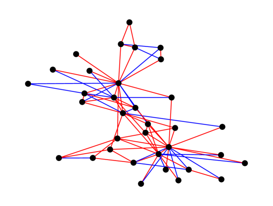
Figure 2: Changes in the normalized edge weights for the FJ model assuming balanced opinions and partitions (Theorem 7) for $T^{*}=\operatorname*{arg\,min}_{T:T\geq\mathbf{0},T\mathbf{1}=\mathbf{1},\mathrm{supp}(T)=G}\mathbb{E}_{s,A}\left[f^{\mathsf{FJ}}(s,A,T)\right]$. The blue (resp. red) edges in the Figure correspond to edges whose weight increased (resp. decreased) in the original graph. The new weights have been found by applying gradient descent using the gradients found in Theorem 7.

In Section 5.1, we calculated $\frac{\partial f^{\mathsf{FJ}}}{\partial w_{e}}$ for an edge $e$. Similarly to previous works such as Wang and Kleinberg (2024), the question that arises here is how changing the weight of a link affects $f^{\mathsf{FJ}}$. We show that under the assumption that the opinions and partitions are balanced, the change in the disparity is always non-positive:

Theorem 7.

If $v\sim\mathcal{N}\left(0,(1/n)I\right)$, $s=|v|$ and $A=\{i\in V:v_{i}\geq 0\}$ and $b_{e}$ is the incidence vector of edge $e$, then

$$\mathbb{E}_{s,A}\left[\frac{\partial f^{\mathsf{FJ}}}{\partial w_{e}}\right]=-\frac{2}{n}b_{e}^{\top}(I+L)^{-3}b_{e}\leq 0.$$

Figure 2 shows the change in the edge weights between the initial graph (degree-normalized weights) and $T^{*}=\operatorname*{arg\,min}_{T:T\geq\mathbf{0},T\mathbf{1}=\mathbf{1},\mathrm{supp}(T)=G}\mathbb{E}_{s,A}\left[f^{\mathsf{FJ}}(s,A,T)\right]$ for the Karate Club network.

7 Experiments

To demonstrate our developed algorithms, we run two experiments on seven real-world social networks: the Karate Club network from Zachary (1984), the Les Miserables network from Knuth (1993), the Caltech and Swarthmore networks from the Facebook100 dataset (Traud et al., 2012), the Political Blogs network from Adamic and Glance (2005), and the Twitter network from Chitra and Musco (2020).

The first experiment focuses on finding the DeGroot weights that minimize disparity (see also Figure 1), assuming that the partition $(A,B)$ is given by running spectral clustering on the initial graph $G$. Except for the Twitter dataset, where initial opinions exist, the initial opinions are sampled uniformly from $[0,1]^{n}$. In Table 1, the total probability mass imbalance defined as $\max\left\{\frac{Q_{A}}{Q_{B}},\frac{Q_{B}}{Q_{A}}\right\}$, as well as the mixing time $t_{\mathrm{mix}}(\varepsilon)=\inf\{k\in\mathbb{N}:\|T^{k}s-q\|_{TV}\leq\varepsilon\}$ for $\varepsilon=10^{-6}$. We observe that the slowest mixing chain corresponds to the Political Blogs dataset which has high cluster imbalance, however we observe that even for small cluster imbalances the mixing times vary greatly.

The second experiment focuses on disparity maximization subject to balanced sentiment, where we find the nodes’ assignment and opinions such as $S_{A}=S_{B}$ (or equivalently $\mathbf{1}^{\top}s=0$). For that experiment, we report the Fiedler value $\lambda_{2}(G)$ and the maximum disparity value $1/(1+\lambda_{2}(G))^{2}$. We observe that the dataset where the highest value of maximum disparity is achieved is the Political Blogs dataset, which, as we would expect, the dataset has a strong cluster structure (see (Adamic and Glance, 2005)). On the other hand, the Karate Club network has the lowest maximum disparity value, corresponding to higher connectivity than the other graphs.

8 Related Work

Opinion Formation. Opinion dynamics have been extensively studied across disciplines such as computer science, economics, sociology, political science, and related fields. Numerous models have been proposed to understand these dynamics, including network interaction-based models like the Friedkin-Johnsen (FJ) model (Friedkin and Cook, 1990; Bindel et al., 2011), bounded confidence dynamics such as the Hegselmann-Krausse Model (Hegselmann et al., 2002), and coevolutionary dynamics (Bhawalkar et al., 2013), along with various extensions; see, for instance, (Abebe et al., 2018; Hazla et al., 2019; Fotakis et al., 2016, 2023; Ristache et al., 2024). In particular, (Bindel et al., 2011) established bounds on the Price of Anarchy (PoA) for the FJ model between the pure Nash equilibria and the welfare-optimal solution, while (Bhawalkar et al., 2013) provided PoA bounds for coevolutionary dynamics. Furthermore, opinion dynamics have been a focus in the control systems literature; see, for example, Nedić and Touri (2012); De Pasquale and Valcher (2022); Bhattacharyya et al. (2013); Chazelle (2011). Our work introduces and studies the disparity metric in the context of the FJ and the DeGroot models.

Polarization and Disagreement in Opinion Dynamics. Our work contributes to the growing literature studying polarization and disagreement in opinion dynamics (Chen and Rácz, 2021; Gaitonde et al., 2020; Musco et al., 2018; Zhu et al., 2021; Chitra and Musco, 2020; Wang and Kleinberg, 2024; Racz and Rigobon, 2022).

Perhaps the most related works are the ones of (Chen and Rácz, 2021) and (Musco et al., 2018) where the authors introduce polarization and disagreement in the context of the FJ model and show how to optimize it, as well as additionally follow up works such as (Wang and Kleinberg, 2024) and (Racz and Rigobon, 2022) which study additional optimization problems on various aspects of the social network (e.g. intrinsic opinions, graph structure, etc.). Our metric contributes to the literature on these metrics and how to optimize them for the intrinsic opinions, the graph, and the groups.

Finally, our work is directly connected to the social science literature regarding the study of polarization – see, for instance, (Garimella et al., 2017, 2018), and the impact of recommendation algorithms in increasing conflict in social networks (Pariser, 2011; Hosanagar et al., 2014; Vaccari et al., 2016; Nguyen et al., 2014; Adamic and Glance, 2005) (also known as the filter-bubble theory), as it gives a way to measure how consensus differs between two groups in a social network.

9 Conclusion

We studied the disparity measure for the DeGroot and FJ opinion dynamics models. For the DeGroot model, minimizing disparity concerning topology or initial opinions is polynomial-time solvable, but finding the optimal partition is NP-Hard. Maximizing disparity can also be solved in polynomial time. For the FJ model, the minimum disparity is independent of graph topology and corresponds to a trivial partition, while the maximum disparity occurs in a complete bipartite graph. We analyzed the effect of assortativity on the minimum disparity in two stochastic block model topologies and showed how to reduce disparity in the FJ model through vertex contractions and link weight adjustments tested on real-world datasets. As a potentially fruitful research direction, we consider the extension to multiple groups (multi-group disparity), extension to multiple correlated graphs or topics, and optimizing disparity in evolving (dynamic) networks.

Acknowledgements

Supported in part by a Simons Investigator Award, a Vannevar Bush Faculty Fellowship, AFOSR grant FA9550-19-1-0183, a Simons Collaboration grant, and a grant from the MacArthur Foundation. MP was partially supported by a LinkedIn Ph.D. Fellowship, a grant from the A.G. Leventis Foundation, a grant from the Gerondelis Foundation, and a scholarship from the Onassis Foundation (Scholarship ID: F ZT 056-1/2023-2024).

Appendix A Ommitted Proofs

A.1 Calculation of $\frac{\partial f^{\mathsf{FJ}}}{\partial w_{e}}$

The proof follows a similar derivation to Wang and Kleinberg [2024]; Musco et al. [2018]. For brevity we set $X=(I+L)^{-1}$. Let $b_{e}$ be the incidence vector to edge $e$. We have

$$\lim_{h\to 0}\frac{1}{h}\left\{(I+L+hbb^{T})^{-2}-X^{2}\right\} =\lim_{h\to 0}\frac{1}{h}\left\{\left(X-\frac{Xbb^{T}X}{1+hb_{e}^{T}Xb_{e}}\right)^{2}-X^{2}\right\}$$

$$=\lim_{h\to 0}\frac{1}{h}\left\{X^{2}-h\frac{X^{2}b_{e}b_{e}^{T}X}{1+hb_{e}^{T}Xb_{e}}-h\frac{Xb_{e}b_{e}^{T}X^{2}}{1+hb_{e}^{T}Xb_{e}}-h^{2}\left[\frac{Xb_{e}b_{e}^{T}X}{1+hb_{e}^{T}Xb_{e}}\right]^{2}-X^{2}\right\}$$

$$=-X(Xb_{e}b_{e}^{T}+b_{e}b_{e}^{T}X)X$$

Therefore

$$\frac{\partial f^{\mathsf{FJ}}}{\partial w_{e}}=-(s_{A}-s_{B})^{\top}(I+L)^{-1}\left[(I+L)^{-1}b_{e}b_{e}^{T}+b_{e}b_{e}^{T}(I+L)^{-1}\right](I+L)^{-1}(s_{A}-s_{B})$$

A.2 Proof of Theorem 1

Let $X=\{x_{1},\dots,x_{m}\}$ be an $m$-element set and $t\geq 0$ be a target for the $(2,t)$-Abs-Partition problem. Without loss of generality, assume that $x_{i}\geq 0$ for all $i\in[m]^{*}$. We build a network $G$ as follows:

• The network $G$ has $n=m$ nodes.

• For every node $i$ we set $s_{i}=1/\sqrt{n}$.

• The principal eigenvector $q$ of the row-stochastic adjacency matrix of $G$ has entries $q_{i}=\frac{x_{i}}{\sum_{j=1}^{n}x_{j}}$, such that $q_{i}\geq 0$ and $\sum_{i=1}^{n}q_{i}=1$. We can choose the other eigenvectors and eigenvalues of the adjacency matrix freely (as long as the adjacency matrix is row-stochastic).

• We set $D=(\sqrt{n}t)/\sum_{i=1}^{n}x_{i}$.

We now prove that the $(2,t)$-Abs-Partition problem has a Yes solution if and only if the $(2,D)$-DeGroot-Disparity problem has a Yes solution. For every valid partition of $X$ into $S$ and $\bar{S}=X\setminus S$ we assign $A=S$ and $B=\bar{S}=V\setminus S$. We therefore get

$$\left|\sum_{i\in S}x_{i}-\sum_{i\in\bar{S}}x_{i}\right|=t\iff\left|\sum_{i\in A}q_{i}-\sum_{i\in B}q_{i}\right|=D.$$ (12)

Therefore a Yes answer to the $(2,t)$-Abs-Partition problem yields a Yes answer to the $(2,D)$-DeGroot-Disparity problem and vice-versa, a Yes answer to the $(2,D)$-DeGroot-Disparity problem yields a Yes answer to the $(2,t)$-Abs-Partition problem.

A.3 Proof of Theorem 2

A.3.1 Algorithm

1. Sort the entries of $q$ in ascending order.

2. Sort the $s_{i}$’s in ascending order.

3. Assign the first $k$ values of $s_{i}$’s to $A$ and the rest $n-k$ values to $B$. Calculate $X_{1}=|q^{\top}(s_{A,1}-s_{B,1})|$ where $s_{A,1},s_{B,1}$ are the resulting opinion vectors for each group after the respective assignment.

4. Assign the first $n-k$ values of $s_{i}$’s to $B$ and the rest $k$ values to $A$. Calculate $X_{2}=|q^{\top}(s_{A,2}-s_{B,2})|$.

5. Output $X=\max\{X_{1},X_{2}\}$ and the corresponding assignment.

A.3.2 Proof

Assume that w.l.o.g. $q_{1}\leq q_{2}\dots\leq q_{n}$, $q=(q_{1},\dots,q_{n})^{\top}$ and $s_{1}\leq s_{2}\dots\leq s_{n}$. Moreover, assume that w.l.o.g. $q^{\top}s_{A}\geq q^{\top}s_{B}$ (the other case is handled symmetrically), where $s_{A},s_{B}$ are to be determined. We create triples $(q_{1},s_{1},x_{1}),(q_{2},s_{2},x_{2}),\dots,(q_{n},s_{n},x_{n})$ where $x_{i}\in\{-1,1\}$ determines whether the $i$-th assignment belongs to group $A$, where $x_{i}=1$ since $q^{\top}s_{A}\geq q^{\top}s_{B}$ or $B$ where $x_{i}=-1$. We prove that the optimal assignment is of the form

$$(q_{1},s_{1},-1),\dots,(q_{k},s_{n-k},-1),$$

$$(q_{n-k+1},s_{n-k+1},1),\dots,(q_{n},s_{n},1)$$

with a value of $V=q^{\top}s_{A}-q^{\top}s_{B}$. Without loss of generality, the $q_{i}$ values will be fixed. We prove that either by perturbing the $s_{i}$’s, the $x_{i}$’s, or both, the objective decreases. We start by perturbing $x_{i}$’s alone. First, this perturbation makes sense only if we change variables between groups and not within the same group (since this violates the rearrangement inequality). Suppose we exchange $x_{i}$ with $x_{j}$ where $i>j$ and $x_{i}x_{j}=-1$ and get a new objective value $X^{\prime}$. The change in the objective is $X-X^{\prime}=q_{i}s_{i}(x_{i}-x_{j})+q_{j}s_{j}(x_{j}-x_{i})=2(q_{i}s_{i}-q_{j}s_{j})\geq 0$ since $q_{i}\geq q_{j}$ and $s_{i}\geq s_{j}$, hence $X^{\prime}\leq X$. Suppose that we exchange the $s_{i}$’s and create an objective value of $X^{\prime\prime}$. Then $X-X^{\prime\prime}=q_{i}s_{i}-q_{i}s_{j}-q_{j}s_{j}+q_{j}s_{i}=(q_{i}+q_{j})(s_{i}-s_{j})\geq 0$ (note the change of signs due to membership), hence $X^{\prime\prime}\leq X$. For the joint perturbation part, perturbing positions $(i,j)$ for $x_{i}$’s and $(i^{\prime},j^{\prime})$ for $s_{i}$’s for $i\neq j$ where $(i,j)\neq(i^{\prime},j^{\prime})$ create a worse objective in the same way as the previous cases separately (since indices are disjoint). The only different case is when the indices are identical, that is $i=i^{\prime}$ and $j=j^{\prime}$, where we have an objective of value $X^{\prime\prime\prime}$. The change in the objective is again $X-X^{\prime\prime\prime}=q_{i}s_{i}x_{i}-q_{i}s_{j}x_{j}+q_{j}s_{j}x_{j}-q_{j}s_{i}x_{i}=(q_{i}-q_{j})(x_{i}s_{i}-x_{j}s_{j})=(q_{i}-q_{j})(s_{i}+s_{j})\geq 0$, since $x_{i}=1$ and $x_{j}=-1$, hence $X^{\prime\prime\prime}\leq X$. Therefore the optimal allocation in this case is to place the first $n-k$ elements to $B$ and the rest $k$ to $A$. The other way around may produce a higher value than $X$, so we take the maximum of the absolute values between these assignments.

A.4 Proof of Corollary 4

The proof is exactly the same as in Theorem 3 of Musco et al. [2018], with the only difference that the $\mathsf{SOL}\leq\frac{1}{(1-\varepsilon)^{2}}\mathsf{OPT}=\left(1+2\varepsilon+O(\varepsilon^{2})\right)\mathsf{OPT}$ for small $\varepsilon$ (i.e. we get $1+2\varepsilon$ approximation instead of $1+\varepsilon$)

A.5 Proof of Theorem 6

Let $H_{1},H_{2}$ be two graphs defined as follows on the vertex set of $G$: $H_{1}$ is the complete graph on $n$ vertices, and $H_{2}\sim\mathcal{G}(n,p)$. First of all, since $H_{1}$ has the largest possible largest eigenvalue of $n$ then $\lambda_{n}(G)\leq\lambda_{n}(H_{1})=n$. For $G$ and $H_{2}$ we prove that w.h.p. $\lambda_{n}(G)\geq\lambda_{n}(H_{2})\geq np-O(1/\ln n)$. The theorem of Chung and Radcliffe [2011] together with the fact that $np/\ln n\to\infty$, that is $H_{2}$ is almost regular, we have that $\lambda_{n}(H_{2})=np\pm O(1/\ln n)$ with probability of at least $1-O(1/n)$. We now couple the graphs $G,H_{2}$ to prove that $\lambda_{n}(G)\geq\lambda_{n}(H_{2})$ almost surely. Let $X_{ij}$ denote the random edges of $G$ and $Y_{ij}$ denote the random edges of $H_{2}$. We define a coupling as follows

1. Whenever $X_{ij}=1$ and $i,j$ are in different groups then $Y_{ij}=1$ with probability $p$.

2. Whenever $X_{ij}=1$ and $i,j$ are in the same group then $Y_{ij}=1$ with probability $p$.

3. Whenever $X_{ij}=0$ then $Y_{ij}=0$.

We can verify that the marginal density of $Y_{ij}$ is

$$\Pr[Y_{ij}=1] =\Pr[X_{ij}=0]\Pr[Y_{ij}=1|X_{ij}=0]$$

$$+\Pr[X_{ij}=1]\Pr[Y_{ij}=1|X_{ij}=1]$$

$$=p.$$

Due to this coupling we can deduce that for all edges we have $Y_{ij}\leq X_{ij}$, hence $H_{2}$ is a subgraph of $G$ under this coupling. Therefore we can state that $\lambda_{n}(G)\geq\lambda_{n}(H_{2})$ almost surely (see Lemma 1. The result is obtained by combining these two inequalities to $np-O(1/\ln n)\leq\lambda_{n}(G)\leq n$, and the rest follows from simultaneous diagonalizeability of $L$ and $(I+L)^{-2}$.

A.6 Proof of Theorem 7

For brevity, let $X=(I+L)^{-1}$ and $y=s_{A}-s_{B}\sim\mathcal{N}(0,(1/n)I)$.

$$\mathbb{E}_{s,A}\left[\frac{\partial f^{\mathsf{FJ}}}{\partial w_{e}}\right] =\mathbb{E}_{y}\left[-y^{\top}X\left[Xb_{e}b_{e}^{\top}+b_{e}b_{e}^{\top}X\right]Xy\right]$$

$$=\mathbb{E}_{y}\left[-y^{\top}X^{2}b_{e}b_{e}^{\top}Xy\right]$$

$$-\mathbb{E}_{y}\left[y^{\top}Xb_{e}b_{e}^{\top}X^{2}y\right]$$

$$={-b_{e}^{\top}X^{2}\mathbb{E}_{s,A}\left[yy^{T}\right]Xb_{e}}$$

$$-{b_{e}^{\top}X\mathbb{E}_{s,A}\left[yy^{T}\right]X^{2}b_{e}}$$

$$=-\frac{2}{n}b_{e}^{\top}X^{-3}b_{e}.$$

Since $X$ is simultaneously diagonalizable with $L$, it has eigenvalues $1/(1+\lambda_{i}(G))^{3}\geq 0$ and therefore $-\frac{2}{n}b_{e}^{\top}X^{-3}b_{e}\leq 0$.

Appendix B Additional Regulator Interventions

B.1 Interventions through Vertex Contractions

The first intervention we consider is a vertex contraction. We define a simplification on a network $G(V,E)$ with $n$ vertices, the process of contracting sets of vertices together to form a “simplified” network $G^{\prime}(V^{\prime},E^{\prime})$ with $n^{\prime}\leq n$ vertices. The most simple operation is the contraction of two neighboring vertices $u,v$ to a new vertex $(uv)$ and the replacement of the intrinsic opinions $s_{u}$ and $s_{v}$ with an intrinsic opinion $s_{uv}$. The memberships of $u,v$ can be arbitrary (i.e. they can belong both to the same group or different groups, and the resulting $(uv)$ node can belong to either of the two groups.). We repeat the process until we reach the final form of $G^{\prime}$, where vertices can be clustered into groups. We define $h:[0,1]^{n}\to[0,1]^{n^{\prime}}$ to be a norm-preserving simplifier of the internal opinions if and only if the application of $h$ on $s$ creates groups $A^{\prime},B^{\prime}$ with $s_{A}^{\prime}=h(s)\odot\mathbf{1}_{A^{\prime}}$ and $s_{B}^{\prime}=h(s)\odot\mathbf{1}_{B^{\prime}}$ and $\|h(s)\|=1$. Below, we prove that any norm-preserving simplification of a network $G$ to a network $G^{\prime}$ increases the minimum disparity.

We first prove the following helper lemma:

Lemma 1.

Let $G$ be an undirected weighted graph with non-negative weights and $H$ be a subgraph of $G$. Then for the largest eigenvalue of the Laplacian we have $\lambda_{n}(G)\geq\lambda_{n}(H)$.

Proof.

Let $x$ be a unit length vector, and $E^{\prime}\subseteq E$ be the corresponding edge sets. We have that $\sum_{\{i,j\}\in E}w_{ij}(x_{i}-x_{j})^{2}\geq\sum_{\{i,j\}\in E^{\prime}}w_{ij}(x_{i}-x_{j})^{2}$ since removing positive terms from a sum reduces it. Fixing $y$ to be a unit length eigenvector corresponding to $\lambda_{n}(H)$ we have $\lambda_{n}(H)=\sum_{\{i,j\}\in E^{\prime}}w_{ij}(y_{i}-y_{j})^{2}\leq\sum_{\{i,j\}\in E}w_{ij}(y_{i}-y_{j})^{2}\leq\sup_{\|z\|=1}\sum_{\{i,j\}\in E}w_{ij}(z_{i}-z_{j})^{2}=\lambda_{n}(G)$. ∎

Then, we proceed to prove the theorem:

Theorem 8.

Let $G$ be a network with intrinsic opinions vector $s$ and let $G^{\prime}$ be constructed from $G$ with via applying the norm-preserving operator $h$. Then the minimum disparity in $G^{\prime}$ is at least the minimum disparity in $G$.

Proof.

We will prove our theorem for the contraction of two vertices $u,v\in V$ to a vertex $(uv)\in V^{\prime}$. The result for multiple simplifications will follow inductively. Let $\mathcal{A}(u)$ be the set $\mathcal{A}(u)=\{w\in N(u)|w\in N(u)\cap(N(v)\cup\{v\})\}$. We proceed by deleting the edges of the form $\{(u,w)|w\in\mathcal{A}(u)\}$ and create a new network $\hat{G}(\hat{V}=V,\hat{E})$. The network $\hat{G}$ has $|\hat{E}|\leq|E|$ edges and therefore its largest eigenvalue of the Laplacian satisfies $\lambda_{n}(\hat{G})\leq\lambda_{n}(G)$ [Brouwer and Haemers, 2011, Proposition 3.1.1]. Moreover, in $\hat{G}$ the vertices $u$ and $v$ have vertex disjoint neighborhoods and can be contracted creating $G^{\prime}(V^{\prime},E^{\prime})$ whereas the largest eigenvalues interlace again, that is $\lambda_{n^{\prime}}(G^{\prime})\leq\lambda_{n}(\hat{G})$ Atay and Tuncel [2014]. Therefore $\lambda_{n^{\prime}}(G^{\prime})\leq\lambda_{n}(G)$. Given that $\|s_{A}-s_{B}\|=\|s\|=1$, we get that the minimum disparity in $G$ is achieved when $s_{A}-s_{B}$ is parallel to the eigenvector corresponding to $\lambda_{n}(G)$ and is equal to $1/(1+\lambda_{n}(G))^{2}$. Now, the minimum disparity on $G^{\prime}$ is achieved when $\hat{s}_{A}^{\prime}-\hat{s}_{B}^{\prime}$ is parallel to the eigenvector corresponding to $\lambda_{n^{\prime}}(G^{\prime})$ and has a value equal to $1/(1+\lambda_{n^{\prime}}(G^{\prime}))^{2}\geq 1/(1+\lambda_{n}(G))^{2}$. Since the vectors $s_{A}^{\prime}=h(s)\odot\mathbf{1}_{A^{\prime}}$ and $s_{B}^{\prime}=h(s)\odot\mathbf{1}_{B^{\prime}}$ such that $\|s_{A}^{\prime}-s_{B}^{\prime}\|=\|h(s)\|=R$ are in general not parallel to this vector, optimality implies that

$$(s_{A}^{\prime}-s_{B}^{\prime})^{\top}(I+L^{\prime})^{-2}(s_{A}^{\prime}-s_{B}^{\prime})\geq\frac{1}{(1+\lambda_{n}(G))^{2}}.$$ (13)

∎

References

- Abebe et al. [2018] Rediet Abebe, Jon Kleinberg, David Parkes, and Charalampos E Tsourakakis. Opinion dynamics with varying susceptibility to persuasion. In Proceedings of the 24th ACM SIGKDD International Conference on Knowledge Discovery & Data Mining, pages 1089–1098, 2018.
- Adamic and Glance [2005] Lada A Adamic and Natalie Glance. The political blogosphere and the 2004 us election: divided they blog. In Proceedings of the 3rd international workshop on Link discovery, pages 36–43, 2005.
- Atay and Tuncel [2014] Fatihcan M Atay and Hande Tuncel. On the spectrum of the normalized laplacian for signed graphs: Interlacing, contraction, and replication. Linear Algebra and its Applications, 442:165–177, 2014.
- Bhattacharyya et al. [2013] Arnab Bhattacharyya, Mark Braverman, Bernard Chazelle, and Huy L Nguyen. On the convergence of the hegselmann-krause system. In Proceedings of the 4th conference on Innovations in Theoretical Computer Science, pages 61–66, 2013.
- Bhawalkar et al. [2013] Kshipra Bhawalkar, Sreenivas Gollapudi, and Kamesh Munagala. Coevolutionary opinion formation games. In Proceedings of the forty-fifth annual ACM symposium on Theory of computing, pages 41–50, 2013.
- Bindel et al. [2011] David Bindel, Jon Kleinberg, and Sigal Oren. How bad is forming your own opinion? In 2011 IEEE 52nd Annual Symposium on Foundations of Computer Science, pages 57–66. IEEE, 2011.
- Bindel et al. [2015] David Bindel, Jon Kleinberg, and Sigal Oren. How bad is forming your own opinion? Games and Economic Behavior, 92:248–265, 2015.
- Boyd and Vandenberghe [2004] Stephen Boyd and Lieven Vandenberghe. Convex optimization. Cambridge university press, 2004.
- Boyd et al. [2004] Stephen Boyd, Persi Diaconis, and Lin Xiao. Fastest mixing markov chain on a graph. SIAM review, 46(4):667–689, 2004.
- Brouwer and Haemers [2011] Andries E Brouwer and Willem H Haemers. Spectra of graphs. Springer Science & Business Media, 2011.
- Chazelle [2011] Bernard Chazelle. The total s-energy of a multiagent system. SIAM Journal on Control and Optimization, 49(4):1680–1706, 2011.
- Chen and Rácz [2021] Mayee F Chen and Miklós Z Rácz. An adversarial model of network disruption: Maximizing disagreement and polarization in social networks. IEEE Transactions on Network Science and Engineering, 9(2):728–739, 2021.
- Chitra and Musco [2020] Uthsav Chitra and Christopher Musco. Analyzing the impact of filter bubbles on social network polarization. In Proceedings of the 13th International Conference on Web Search and Data Mining, pages 115–123, 2020.
- Chung and Radcliffe [2011] Fan Chung and Mary Radcliffe. On the spectra of general random graphs. the electronic journal of combinatorics, pages P215–P215, 2011.
- De Pasquale and Valcher [2022] Giulia De Pasquale and Maria Elena Valcher. Multi-dimensional extensions of the hegselmann-krause model. In 2022 IEEE 61st Conference on Decision and Control (CDC), pages 3525–3530. IEEE, 2022.
- DeGroot [1974] Morris H DeGroot. Reaching a consensus. Journal of the American Statistical association, 69(345):118–121, 1974.
- Fotakis et al. [2016] Dimitris Fotakis, Dimitris Palyvos-Giannas, and Stratis Skoulakis. Opinion dynamics with local interactions. In IJCAI, pages 279–285, 2016.
- Fotakis et al. [2023] Dimitris Fotakis, Vardis Kandiros, Vasilis Kontonis, and Stratis Skoulakis. Opinion dynamics with limited information. Algorithmica, 85(12):3855–3888, 2023.
- Friedkin and Cook [1990] Noah E Friedkin and Karen S Cook. Peer group influence. Sociological Methods & Research, 19(1):122–143, 1990.
- Friedkin and Johnsen [1990] Noah E Friedkin and Eugene C Johnsen. Social influence and opinions. Journal of Mathematical Sociology, 15(3-4):193–206, 1990.
- Gaitonde et al. [2020] Jason Gaitonde, Jon Kleinberg, and Eva Tardos. Adversarial perturbations of opinion dynamics in networks. In Proceedings of the 21st ACM Conference on Economics and Computation, pages 471–472, 2020.
- Gaitonde et al. [2021] Jason Gaitonde, Jon Kleinberg, and Éva Tardos. Polarization in geometric opinion dynamics. In Proceedings of the 22nd ACM Conference on Economics and Computation, pages 499–519, 2021.
- Garimella et al. [2017] Kiran Garimella, Gianmarco De Francisci Morales, Aristides Gionis, and Michael Mathioudakis. Reducing controversy by connecting opposing views. In Proceedings of the Tenth ACM International Conference on Web Search and Data Mining, pages 81–90, 2017.
- Garimella et al. [2018] Kiran Garimella, Gianmarco De Francisci Morales, Aristides Gionis, and Michael Mathioudakis. Quantifying controversy on social media. ACM Transactions on Social Computing, 1(1):1–27, 2018.
- Gionis et al. [2013] Aristides Gionis, Evimaria Terzi, and Panayiotis Tsaparas. Opinion maximization in social networks. In Proceedings of the 2013 SIAM International Conference on Data Mining, pages 387–395. SIAM, 2013.
- Hazla et al. [2019] Jan Hazla, Yan Jin, Elchanan Mossel, and Govind Ramnarayan. A geometric model of opinion polarization. arXiv preprint arXiv:1910.05274, 2019.
- Hegselmann et al. [2002] Rainer Hegselmann, Ulrich Krause, et al. Opinion dynamics and bounded confidence models, analysis, and simulation. Journal of artificial societies and social simulation, 5(3), 2002.
- Hosanagar et al. [2014] Kartik Hosanagar, Daniel Fleder, Dokyun Lee, and Andreas Buja. Will the global village fracture into tribes? recommender systems and their effects on consumer fragmentation. Management Science, 60(4):805–823, 2014.
- Kellerer et al. [2003] Hans Kellerer, Renata Mansini, Ulrich Pferschy, and Maria Grazia Speranza. An efficient fully polynomial approximation scheme for the subset-sum problem. Journal of Computer and System Sciences, 66(2):349–370, 2003.
- Knuth [1993] Donald Ervin Knuth. The Stanford GraphBase: a platform for combinatorial computing, volume 1. AcM Press New York, 1993.
- Musco et al. [2018] Cameron Musco, Christopher Musco, and Charalampos E Tsourakakis. Minimizing polarization and disagreement in social networks. In Proceedings of the 2018 world wide web conference, pages 369–378, 2018.
- Nedić and Touri [2012] Angelia Nedić and Behrouz Touri. Multi-dimensional hegselmann-krause dynamics. In 2012 IEEE 51st IEEE Conference on Decision and Control (CDC), pages 68–73. IEEE, 2012.
- Nguyen et al. [2014] Tien T Nguyen, Pik-Mai Hui, F Maxwell Harper, Loren Terveen, and Joseph A Konstan. Exploring the filter bubble: the effect of using recommender systems on content diversity. In Proceedings of the 23rd international conference on World wide web, pages 677–686, 2014.
- Pariser [2011] Eli Pariser. The filter bubble: How the new personalized web is changing what we read and how we think. Penguin, 2011.
- Racz and Rigobon [2022] Miklos Z Racz and Daniel E Rigobon. Towards consensus: Reducing polarization by perturbing social networks. arXiv preprint arXiv:2206.08996, 2022.
- Ristache et al. [2024] Dragos Ristache, Fabian Spaeh, and Charalampos E Tsourakakis. Wiser than the wisest of crowds: The asch effect and polarization revisited. In Joint European Conference on Machine Learning and Knowledge Discovery in Databases, pages 440–458. Springer, 2024.
- Spielman and Srivastava [2008] Daniel A Spielman and Nikhil Srivastava. Graph sparsification by effective resistances. In Proceedings of the fortieth annual ACM symposium on Theory of computing, pages 563–568, 2008.
- Traud et al. [2012] Amanda L Traud, Peter J Mucha, and Mason A Porter. Social structure of facebook networks. Physica A: Statistical Mechanics and its Applications, 391(16):4165–4180, 2012.
- Vaccari et al. [2016] Cristian Vaccari, Augusto Valeriani, Pablo Barberá, John T Jost, Jonathan Nagler, and Joshua A Tucker. Of echo chambers and contrarian clubs: Exposure to political disagreement among german and italian users of twitter. Social media+ society, 2(3):2056305116664221, 2016.
- Wang and Kleinberg [2024] Yanbang Wang and Jon Kleinberg. On the relationship between relevance and conflict in online social link recommendations. Advances in Neural Information Processing Systems, 36, 2024.
- Zachary [1984] Wayne W Zachary. Modeling social network processes using constrained flow representations. Social Networks, 6(3):259–292, 1984.
- Zhang et al. [2015] Xiao Zhang, Travis Martin, and Mark EJ Newman. Identification of core-periphery structure in networks. Physical Review E, 91(3):032803, 2015.
- Zhu et al. [2021] Liwang Zhu, Qi Bao, and Zhongzhi Zhang. Minimizing polarization and disagreement in social networks via link recommendation. Advances in Neural Information Processing Systems, 34:2072–2084, 2021.