Enabling Gigantic MIMO Beamforming
with Analog Computing
††thanks: This work has been partially supported by UKRI grant EP/Y004086/1, EP/X040569/1, EP/Y037197/1, EP/X04047X/1, and EP/Y037243/1.
Abstract
In our previous work, we have introduced a microwave linear analog computer (MiLAC) as an analog computer that processes microwave signals linearly, demonstrating its potential to reduce the computational complexity of specific signal processing tasks. In this paper, we extend these benefits to wireless communications, showcasing how MiLAC enables gigantic multiple-input multiple-output (MIMO) beamforming entirely in the analog domain. MiLAC-aided beamforming can implement regularized zero-forcing beamforming (R-ZFBF) at the transmitter and minimum mean square error (MMSE) detection at the receiver, while significantly reducing hardware costs by minimizing the number of radio-frequency (RF) chains and only relying on low-resolution analog-to-digital converters (ADCs) and digital-to-analog converters (DACs). In addition, it eliminates per-symbol operations by completely avoiding digital-domain processing and remarkably reduces the computational complexity of R-ZFBF, which scales quadratically with the number of antennas instead of cubically. Numerical results show that it can perform R-ZFBF with a computational complexity reduction of up to 7400 times compared to digital beamforming.
Index Terms:
Analog computing, gigantic multiple-input multiple-output (MIMO), minimum mean square error (MMSE), zero-forcing (ZF).I Introduction
Future wireless systems are expected to require a significantly larger number of antennas to support higher data rates and simultaneously serve a larger number of users. While massive multiple-input multiple-output (MIMO) systems typically deploy 64 or more antennas [1, 2], this number could reach several thousands in ultra-massive or gigantic MIMO systems, which have been recently proposed to meet the stringent requirements of 6G networks [3]. With such a large number of antennas, digital beamforming faces two critical challenges in terms of hardware and computational complexity. First, digital beamforming typically requires a dedicated radio-frequency (RF) chain per antenna element, each including analog-to-digital converters (ADCs)/digital-to-analog converters (DACs) and mixers, which are costly and power-hungry components. Second, as the number of antennas increases, the data volumes to be processed in real-time grow accordingly. For example, to precode the transmitted symbol vector at the transmitter (or combine the received symbol vector at the receiver) a matrix-vector product is required on a per-symbol basis. These two challenges result in high hardware costs and computational complexity when digital beamforming is applied in massive or gigantic MIMO systems. For these reasons, several alternatives to digital beamforming have been explored to enable beamforming operations fully or partially in the analog domain.
To address the high hardware cost associated with digital beamforming, alternative beamforming strategies have been proposed. Analog beamforming steers the beam pattern by solely requiring a single RF chain [4]. This is achieved by connecting the RF chain to the antennas via phase shifters or time delay elements, which impose a constant modulus constraint on the beamforming weights. To balance hardware cost and flexibility by bridging analog and digital beamforming, hybrid analog-digital beamforming techniques have been widely investigated [4, 5, 6]. Another method to efficiently perform beamforming in the analog domain is given by reconfigurable intelligent surface (RIS) [7, 8]. This technology has recently emerged enabling the control of the wireless channel through surfaces made of multiple passive elements with reconfigurable scattering properties. Beamforming in the analog domain can be achieved through RIS by deploying a RIS in close proximity to an active transceiving device equipped with a reduced number of antennas. In this way, the effective radiation pattern of the active device can be optimized by reconfiguring the RIS elements [9, 10, 11]. Two extensions of this technology have been proposed to achieve additional flexibility over conventional RIS, such as beyond diagonal RIS (BD-RIS) [12] and stacked intelligent metasurface (SIM) [13]. The additional flexibility provided by BD-RIS and the multiple layers in SIM has shown increased performance over just deploying a single conventional RIS.
Numerous technologies have been proposed to reduce the hardware cost of future wireless transceivers by executing beamforming in the analog domain [4]-[13]. However, the use of analog beamforming strategies to alleviate the computational complexity of future wireless networks has received limited attention [14]. In this paper, we address this gap by proposing a novel beamforming strategy enabled by the concept of microwave linear analog computer (MiLAC), recently introduced in [15]. This beamforming strategy, which operates entirely in the analog domain, reduces the hardware cost by minimizing the number of required RF chains and relying only on low-resolution ADCs/DACs. By leveraging the computational capabilities of MiLACs, it also minimizes the computational complexity required for beamforming.
The contributions of this paper can be summarized as follows. First, we demonstrate that a MiLAC can efficiently compute regularized least squares (RLS), with significantly reduced computational complexity compared to conventional digital computing. Second, we propose MiLAC-aided beamforming as a new beamforming strategy enabled by MiLAC scalable to gigantic MIMO systems. MiLAC-aided beamforming allows us to perform regularized zero-forcing beamforming (R-ZFBF) at the transmitter and minimum mean square error (MMSE) detection at the receiver in the analog domain, with important gains in terms of both hardware and computational complexity. Third, we provide numerical results to assess the performance of MiLAC-aided beamforming in terms of sum rate, confirming that it can achieve the same performance as digital beamforming. We also assess the benefits of MiLAC-aided beamforming over digital beamforming in terms of computational complexity, showing that it can perform R-ZFBF with a gain in computational complexity of times. Thus, in a gigantic MIMO system with thousands of antennas, MiLAC-aided beamforming achieves the same performance as digital R-ZFBF at just th of the computational cost. From a different perspective, a 4096-antenna MiLAC serving 4096 users via R-ZFBF requires the same computational complexity as a 256-antenna digital transmitter serving 256 users. This makes MiLAC-aided beamforming a game changer for gigantic MIMO, opening the door to radically new transceiver architectures that can massively scale the number of antennas and users.
Notation: Vectors and matrices are denoted with bold lower and bold upper letters, respectively. Scalars are represented with letters not in bold font. , , , and refer to the transpose, conjugate transpose, th element, and -norm of a vector , respectively. , , , , and refer to the transpose, conjugate transpose, th element, th column, and Frobenius norm of a matrix , respectively. and denote the real and complex number sets, respectively. denotes the imaginary unit. and denote the identity matrix and the all-zero matrix with dimensions , respectively, and denote the all-zero matrix with dimensions .
II Microwave Linear Analog Computer
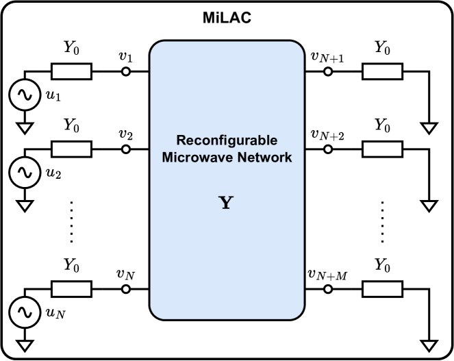
In this section, we briefly review the concept of MiLAC, defined as an analog computer that linearly processes microwave signals, as introduced in [15]. In general, a MiLAC can be seen as a -port reconfigurable microwave network, which can be characterized by its admittance matrix . We assume this microwave network to be made of tunable admittance components interconnecting each port to ground and to all the other ports, such that the microwave network can be reconfigured to assume any arbitrary admittance matrix . The admittance component interconnecting port to ground is denoted as , for , while the admittance component interconnecting port to port is denoted as , for . The input signal is applied by voltage generators with series admittance to the first ports of the MiLAC, with , as represented in Fig. 1. The output signal is read on all ports, where with denoting the number of ports with no input, and is denoted by , as shown in Fig. 1. For convenience of representation, we introduce the output vectors and as and , such that .
It has been shown in [15] that the output vectors and can be expressed as a function of the admittance matrix and the input by introducing a matrix as
| (1) |
partitioned as
| (2) |
where , , , and . Assuming to be invertible, with or invertible, and are expressed depending on the invertibility of and as follows:
-
1.
If is invertible, we have
(3) (4) -
2.
If is invertible, we have
(5) (6) - 3.
Note that (3)-(4) and (5)-(6) express the output vectors and as a function of the input and the blocks of , which are directly related to by (1). The expressions (3)-(4) and (5)-(6) can be computed by a MiLAC given any blocks , , , and by setting the tunable admittance components as a function of any arbitrary as
| (7) |
for , as discussed in [15]. Remarkably, a MiLAC can efficiently compute (3)-(4) and (5)-(6) in the analog domain, while they would require computationally expensive matrix-matrix products and matrix inversion operations if digitally computed.
| LMMSE | ||
|---|---|---|
| RLS |
III Analog Computing for
Regularized Least Squares
In [15], we have shown how a MiLAC can be used to compute the linear minimum mean square error (LMMSE) estimator of a linear observation process with reduced computational complexity. In this section, we demonstrate that a MiLAC can also efficiently compute RLS in the analog domain, an operation of particular interest in wireless communications. This is achieved by first recalling the concept of LMMSE estimator and showing that it includes RLS as a special case.
Consider a linear observation process , where is the observation vector, is a known constant matrix, is the unknown random vector with mean and covariance matrix , and is the random noise vector with mean and covariance matrix . As discussed in [15], the LMMSE estimator of is equivalently given by
| (8) | ||||
| (9) |
when and are both invertible, which holds true in general.
This LMMSE estimator has been obtained with no assumptions on the covariance matrices and beyond their invertibility. With specific assumptions on and , we can show that it includes the RLS, also known as ridge regression, as a special case of practical interest. Specifically, assume that the entries of and are uncorrelated and have equal variance, i.e., and , with and . Thus, by introducing such that , (8) and (9) simplify as
| (10) | ||||
| (11) |
respectively, which are known as the expressions of RLS. Interestingly, the expressions in (10) and (11) are widely used in MIMO wireless communications to realize the so-called R-ZFBF at the transmitter and MMSE detection at the receiver, as effective linear transmission and reception techniques, respectively [16, Chapters 7, 12].
The expressions of RLS can be efficiently returned on the output vector of a MiLAC having input ports and output ports with no input, i.e., total ports. This is achieved by exploiting (4) and (6), as discussed for the LMMSE estimator in [15]. The input vector of the MiLAC is set as and the tunable admittance components are set according to (7) such that the blocks of the matrix give the desired expression in . In detail, the RLS expressions in (10) and (11) can be computed by setting the matrix as illustrated in Tabs. I and II.
| LMMSE | ||
|---|---|---|
| RLS |
Remark 1.
RLS, or ridge regression, can be efficiently computed using a MiLAC, which offers significantly reduced computational complexity compared to a digital computer. This is because a MiLAC directly performs matrix-matrix multiplications and matrix inversion operations in the analog domain. On the one hand, the computational complexity of computing RLS with a MiLAC is driven by the complexity of computing (7) for a given matrix . Thus, the complexity required to compute RLS with a MiLAC is the same as the complexity of computing the LMMSE estimator, i.e., real operations, as discussed in [15]. On the other hand, a digital computer calculates the RLS with a complexity of real operations as it requires one matrix-matrix product and a matrix inversion (see [15, Appendix] for more details on the complexity of a matrix-matrix product and a matrix inversion).
IV A Novel Beamforming Strategy:
MiLAC-Aided Beamforming
In this section, we show how a MiLAC can be used to implement a novel beamforming technique, that we denote as MiLAC-aided beamforming, at the transmitter as well as receiver side. MiLAC-aided beamforming offers circuit and computational complexity benefits by fully operating in the analog domain. To illustrate MiLAC-aided beamforming, we consider a MIMO communication system between transmitting antennas and receiving antennas through the wireless channel . We denote as the transmitted signal and as the received signal such that , where is the additive white Gaussian noise (AWGN) 111We consider here a general MIMO system, such as single-user MIMO or multi-user with one symbol per user. Both single- and multi-user systems will be specifically studied in the following subsections..
IV-A R-ZFBF at the Transmitter
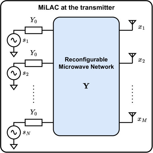
Assume that the MIMO system is a multi-user system between an -antenna transmitter and single-antenna users, with . The signal received at the users is used to detect the symbols , with , and the transmitted signal is given by , where is the precoding matrix. Such a transmitter can be implemented purely in the analog domain by a MiLAC having ports receiving the symbol vector in input and ports delivering the output to antennas perfectly matched to the reference impedance , as represented in Fig. 2. Since the antennas are perfectly matched, their Thevenin equivalent circuit is an impedance connected to ground [17, Chapter 2.13]. Thus, the MiLAC in Fig. 2 behaves as when its last ports are connected to ground through an impedance , i.e., as analyzed in Section II. By exploiting Tab. II, it is possible to reconfigure the microwave network of the MiLAC to efficiently execute R-ZFBF [16, Chapter 12]. Specifically, a MiLAC computing RLS can realize R-ZFBF, with precoding matrix , where is an arbitrary regularization factor. This can be obtained by reconfiguring the tunable admittance components of the MiLAC according to the channel on a per coherence block basis, and do not require any operation on a per-symbol basis.
Remark 2.
According to Remark 1, R-ZFBF can be achieved with only real operations, which are necessary to set the tunable admittance components of the MiLAC. Conversely, the computational complexity of digitally calculating the R-ZFBF matrix is real operations. This confirms the significant benefits of MiLAC-aided beamforming in terms of computational complexity.
IV-B MMSE at the Receiver
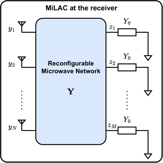
As discussed on the transmitter side, MiLAC-aided beamforming can also be introduced on the receiver side. Assume that the MIMO system is a single-user system between an -antenna transmitter and a -antenna receiver, with . The transmitted signal contains the symbols to be detected at the receiver, i.e., , and the receiver uses the signal to accurately detect the symbols, where is the combining matrix. This receiver can be implemented with MiLAC having ports acquiring the input from the receiving antennas and ports providing the output vector , as represented in Fig. 3. Note that in Fig. 3 we assume the antennas to be perfectly matched to the reference impedance , such that their Thevenin equivalent circuit is a voltage generator (inducing a voltage at port , for ) in series to an impedance [17, Chapter 2.13], i.e., as in the MiLAC analyzed in Section II. By using Tab. I, it is possible to reconfigure the microwave network of the MiLAC to efficiently the MMSE receiver [16, Chapter 7]. Specifically, a MiLAC computing RLS can realize the MMSE receiver with combining matrix . If the covariance matrix of the transmitted signal is , where is the transmit power, and the covariance matrix of the noise is , where is the noise power, the optimal regularization factor is given by [16, Chapter 7]. This can be realized by solely reconfiguring the MiLAC on a per coherence block basis, while no operation is required on a per-symbol basis.
Remark 3.
Similarly to Remark 2, MMSE detection at the receiver can be obtained through a MiLAC with only real operations, which are required to set the tunable admittance components. In contrast, the computational complexity of digitally calculating MMSE detection is real operations, showing important benefits in using MiLAC-aided beamforming to implement MMSE detection.
IV-C Benefits of MiLAC-Aided Beamforming
We have discussed how a MiLAC can enable R-ZFBF at the transmitter and MMSE at the receiver purely in the analog domain. We now highlight the benefits of MiLAC-aided beamforming, showing that it requires the lowest number of RF chains, low-resolution ADCs/DACs, and highly reduced computational complexity. The following discussion for a transmitter readily applies also at the receiver side.
IV-C1 Minimum Number of RF Chains
In MiLAC-aided beamforming, the symbols are fed in input to the MiLAC, which computes the transmitted signal in the analog domain. Thus, only RF chains are needed to achieve R-ZFBF, which is the minimum number of RF chains requested by conventional beamforming strategies.
IV-C2 Low-resolution ADCs/DACs
Since MiLAC-aided beamforming processes the symbols purely in the analog domain, each RF chain carries an individual symbol, which lies in a constellation with finite cardinality. Thus, low-resolution ADCs/DACs can be adopted without sacrificing performance, which are less expensive and less power-hungry than high-resolution ADCs/DACs. High-resolution ADCs/DACs are instead necessary when beamforming is performed in the digital domain (entirely or in part), i.e., in digital beamforming, hybrid beamforming, and RIS-aided beamforming.
IV-C3 No Computations on a Per-Symbol Basis
If beamforming is performed in the digital domain (entirely or in part), the matrix-vector product needs to be computed on a per-symbol basis. The complexity of this operation is real operations, where is the number of RF chains, as discussed in [15, Appendix], and can become prohibitive in massive/gigantic MIMO systems [2]. MiLAC-aided beamforming solves this issue since it does not require any computation on a per-symbol basis, as the beamforming is purely analog. This reduces the beamforming computational complexity, especially when the coherence time is much longer than the symbol time [2].
IV-C4 Minimum Computations Per Coherence Block
MiLAC-aided beamforming offers further gains in terms of computational complexity by exploiting the capability of a MiLAC to efficiently compute RLS in the analog domain.
V Numerical Results
We have proposed MiLAC-aided beamforming as a novel beamforming strategy that offers promising advantages in terms of circuit and computational complexity. In this section, we evaluate the performance and computational complexity of MiLAC-aided beamforming when it is used for R-ZFBF.
Consider a multi-user multiple-input single-output (MISO) system with an -antenna transmitter and single-antenna receivers, as presented in Section IV-A. Here, the transmitter precodes the symbols intended to the receivers through R-ZFBF. With digital beamforming, the R-ZFBF transmitter is realized by computing and setting the precoding matrix such that , for , assuming uniform power allocation to the users. For large and if the signal-to-noise ratio (SNR) is the same at all receiving antennas, the optimal is , where is the transmit power, i.e., has covariance matrix , is the noise power, and we assumed the channel to have unit path gain [16, Chapter 12]. With MiLAC-aided beamforming, the MiLAC can directly compute the R-ZFBF matrix in the analog domain, as explained in Section IV-A. In this case, the columns of cannot be individually normalized, and the resulting precoding matrix is given by , where the normalization factor has been included to ensure that the transmit power is the same as with digital beamforming.
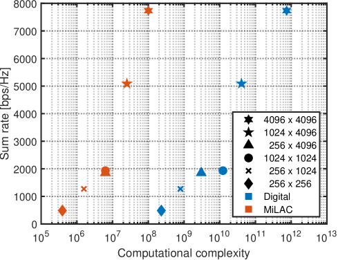
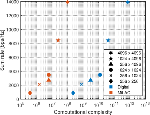
In the considered system, the beamforming matrix is reconfigured per coherence block, where each coherence block includes symbol transmissions. We define the computational complexity as the number of real operations per coherence block. For R-ZFBF at the transmitter, MiLAC-aided beamforming requires operations per coherence block, as specified in Remark 2, and no operation is required on a per-symbol basis. Conversely, with digital beamforming, R-ZFBF requires operations to design the beamforming matrix at each coherence block (see Remark 2). In addition, the matrix-vector product is performed on a per-symbol basis, requiring real operations per symbol time and making the complexity per coherence block of digital beamforming .
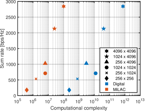
In Fig. 4, we report the achieved sum rate and required computational complexity for MiLAC-aided and digital R-ZFBF beamforming in the case of different values of and , where and , and SNR , where dB, by fixing symbols per coherence block. The values are averaged over multiple realizations of independent and identically distributed (i.i.d.) Rayleigh distributed channels with unit path gain. We make the following three observations. First, the sum rate increases with the number of transmit antennas , the number of receivers , and the SNR, for both MiLAC-aided and digital beamforming. Besides, the computational complexity increases with the number of transmit antennas and receivers , for both MiLAC-aided and digital beamforming, while is independent of the SNR. Second, with a high number of transmit antennas, i.e., , the performance achieved by a MiLAC computing the R-ZFBF matrix in the analog domain as per Section IV-A is the same as with digital beamforming with uniform power allocation. Thus, we can fully exploit the computational benefits of MiLAC-aided beamforming without sacrificing performance. Third, MiLAC-aided beamforming offers the same performance as digital beamforming for all the considered configurations of , , and SNR, with significant gains in computational complexity, up to times when . Under a different perspective, MiLAC-aided beamforming can significantly improve the sum rate over digital beamforming given the same computational complexity. For example, MiLAC-aided beamforming can operate R-ZFBF in a system with requiring approximately the same complexity as digital R-ZFBF in a system with .
VI Conclusion
In this paper, we demonstrate the application of MiLAC to wireless communications, highlighting its potential to support communications with thousands of antennas by enabling analog-domain computations and beamforming. We first derive RLS as a special case of the LMMSE estimator that has a practical interest in wireless communications, and illustrate how it can be computed by a MiLAC in the analog domain. Following the capability of a MiLAC to compute RLS, we introduce MiLAC-aided beamforming as a novel beamforming strategy enabled by a MiLAC. Compared to state-of-the-art beamforming strategies, MiLAC-aided beamforming offers unique benefits in terms of hardware and computational complexity. Numerical results support the theoretical insights, showing that MiLAC-aided beamforming can perform R-ZFBF with a remarkable reduction in computational complexity, i.e., up times.
References
- [1] E. G. Larsson, O. Edfors, F. Tufvesson, and T. L. Marzetta, “Massive MIMO for next generation wireless systems,” IEEE Commun. Mag., vol. 52, no. 2, pp. 186–195, 2014.
- [2] E. Björnson, E. G. Larsson, and T. L. Marzetta, “Massive MIMO: Ten myths and one critical question,” IEEE Commun. Mag., vol. 54, no. 2, pp. 114–123, 2016.
- [3] E. Björnson, F. Kara, N. Kolomvakis, A. Kosasih, P. Ramezani, and M. B. Salman, “Enabling 6G performance in the upper mid-band by transitioning from massive to gigantic MIMO,” arXiv preprint arXiv:2407.05630, 2024.
- [4] S. Sun, T. S. Rappaport, R. W. Heath, A. Nix, and S. Rangan, “MIMO for millimeter-wave wireless communications: Beamforming, spatial multiplexing, or both?” IEEE Commun. Mag., vol. 52, no. 12, pp. 110–121, 2014.
- [5] O. E. Ayach, S. Rajagopal, S. Abu-Surra, Z. Pi, and R. W. Heath, “Spatially sparse precoding in millimeter wave MIMO systems,” IEEE Trans. Wireless Commun., vol. 13, no. 3, pp. 1499–1513, 2014.
- [6] F. Sohrabi and W. Yu, “Hybrid digital and analog beamforming design for large-scale antenna arrays,” IEEE J. Sel. Top. Signal Process., vol. 10, no. 3, pp. 501–513, 2016.
- [7] M. Di Renzo, A. Zappone, M. Debbah, M.-S. Alouini, C. Yuen, J. de Rosny, and S. Tretyakov, “Smart radio environments empowered by reconfigurable intelligent surfaces: How it works, state of research, and the road ahead,” IEEE J. Sel. Areas Commun., vol. 38, no. 11, pp. 2450–2525, 2020.
- [8] Q. Wu, S. Zhang, B. Zheng, C. You, and R. Zhang, “Intelligent reflecting surface-aided wireless communications: A tutorial,” IEEE Trans. Commun., vol. 69, no. 5, pp. 3313–3351, 2021.
- [9] V. Jamali, A. M. Tulino, G. Fischer, R. R. Müller, and R. Schober, “Intelligent surface-aided transmitter architectures for millimeter-wave ultra massive MIMO systems,” IEEE Open J. Commun. Soc., vol. 2, pp. 144–167, 2021.
- [10] C. You, B. Zheng, W. Mei, and R. Zhang, “How to deploy intelligent reflecting surfaces in wireless network: BS-side, user-side, or both sides?” J. Commun. Inf. Netw., vol. 7, no. 1, pp. 1–10, 2022.
- [11] Y. Huang, L. Zhu, and R. Zhang, “Integrating intelligent reflecting surface into base station: Architecture, channel model, and passive reflection design,” IEEE Trans. Commun., vol. 71, no. 8, pp. 5005–5020, 2023.
- [12] S. Shen, B. Clerckx, and R. Murch, “Modeling and architecture design of reconfigurable intelligent surfaces using scattering parameter network analysis,” IEEE Trans. Wireless Commun., vol. 21, no. 2, pp. 1229–1243, 2022.
- [13] J. An, C. Xu, D. W. K. Ng, G. C. Alexandropoulos, C. Huang, C. Yuen, and L. Hanzo, “Stacked intelligent metasurfaces for efficient holographic MIMO communications in 6G,” IEEE J. Sel. Areas Commun., vol. 41, no. 8, pp. 2380–2396, 2023.
- [14] P. Mannocci, E. Melacarne, and D. Ielmini, “An analogue in-memory ridge regression circuit with application to massive MIMO acceleration,” IEEE J. Emerg. Sel. Top. Circuits Syst., vol. 12, no. 4, pp. 952–962, 2022.
- [15] M. Nerini and B. Clerckx, “Analog computing with microwave networks,” arXiv preprint arXiv:2504.06790, 2025.
- [16] B. Clerckx and C. Oestges, MIMO wireless networks: Channels, techniques and standards for multi-antenna, multi-user and multi-cell systems. Academic Press, 2013.
- [17] C. A. Balanis, Antenna theory: Analysis and design. John Wiley & Sons, 2015.