Dynamical quantum phase transition, metastable state, and dimensionality reduction: Krylov analysis of fully-connected spin models

Abstract

We study quenched dynamics of fully-connected spin models. The system is prepared in a ground state of the initial Hamiltonian and the Hamiltonian is suddenly changed to a different form. We apply the Krylov subspace method to map the system onto an effective tridiagonal Hamiltonian. The state is confined in a potential well and is time-evolved by nonuniform hoppings. The dynamical singularities for the survival probability can occur when the state is reflected from a potential barrier. Although we do not observe any singularity in the spread complexity, we find that the entropy exhibits small dips at the singular times. We find that the presence of metastable state affects long-time behavior of the spread complexity, and physical observables. We also observe a reduction of the state-space dimension when the Hamiltonian reduces to a classical form.

I Introduction

Nonequilibrium dynamics in quantum many-body systems has emerged as a central theme in quantum algorithms and condensed matter physics [1, 2, 3, 4]. In particular, quantum quenches where a system is prepared in an initial state and then subjected to a sudden change in the Hamiltonian, serve as a fundamental protocol for studying nonequilibrium physics. The response of a system to such abrupt changes not only reveals fundamental properties of quantum many-body systems but also provides crucial insights into quantum information propagation and thermalization mechanisms.

It is known that a certain kind of quenched systems exhibits dynamical quantum phase transitions (DQPTs) [5, 6, 7, 8, 9]. When we consider quenches across an equilibrium quantum phase transition, the rate function of the survival probability as a function of time shows nonanalytic behavior at the thermodynamic limit. Various quench patterns lead to various behaviors in real-time evolutions that cannot be seen in the corresponding equilibrium system. Some of the properties are described by the analytic studies of specific exactly solvable models.

In the present study, we describe a quenched system with respect to the Krylov subspace method [10, 11]. The quenched dynamics is set by specifying the Hamiltonian and the initial state. Since this setting is completely the same as that in the Krylov subspace method, the application of the method is a reasonable strategy. The advantage of the Krylov subspace method is that any system can be mapped onto a one-dimensional hopping model. The tridiagonal form of the effective Hamiltonian reflects the initial setting of the quench protocol. Then, it would be interesting to describe the DQPT with respect to the Krylov terminology. The Krylov subspace method has attracted renewed interests as a method for describing universal properties of operator growth [12, 13]. To quantify the concept of operator complexity, the authors in Ref. [12] introduced the Krylov complexity measuring how far the time-evolved Heisenberg operator is from the initial operator. The same consideration is applied to the time-evolved state and we can define the spread complexity to quantify the state spreading [14].

As a simple model showing the DQPT, we exploit a fully-connected spin Hamiltonian. The quenched Lipkin–Meshkov–Glick (LMG) model [15] is one of the models that exhibit the DQPT [16, 17]. As shown in Ref. [17], the singularities can be best seen in systems with a bias field that breaks spin-reflection symmetry. Although there exist several preceding studies of the LMG model by the Krylov subspace method [18, 19, 20], and by the non-Krylov complexity analysis [21], the bias field was not introduced there. Here, we analyze the LMG model with the bias field. The main aim of the present study is to see how the DQPT is described in Krylov space. We find that, in the picture of one-dimensional Krylov lattice, the DQPT can occur when the state is reflected from a potential barrier. Since the hopping amplitude is nonuniform, this one-dimensional picture incorporates nontrivial effects. Similar Krylov studies were recently done for Ising models [22, 23, 24].

In principle, the DQPT occurs only in the thermodynamic limit. Although they appear repeatedly in the time sequence of the survival probability, the amplitude typically shows decaying behavior, which leads to smearing of singularities. It is generally difficult to know the long-time behavior of the system, both theoretically and experimentally. Theoretically, the long-time behavior is strongly dependent on the system size and it is hard to know the thermodynamic limit. In the present study, we introduce the bias field. It explicitly breaks spin-reflection symmetry and makes the system more in a trivial state. However, a small bias field produces a metastable state, which makes the dynamical behavior nontrivial. While the metastable state does not affect the statistical-mechanical properties at the thermodynamic limit, it does dynamical properties significantly. We find that the long-time behavior is unstable and is sensitive to the parameter choice.

The organization of this paper is as follows. In Sec. II we introduce the model system, summarize the known results, and describe our strategy. Next, in Sec. III, we study dynamical singularities by using the Krylov subspace method. We also discuss metastable state in Sec. IV and dimensionality reduction in Sec. V. The last section VI is devoted to conclusions.

II Krylov subspace method for the LMG model

II.1 DQPT and Krylov subspace method

In the standard framework of closed quantum systems, we prepare a initial state $|\psi_{0}\rangle$ and consider the time evolution

$$|\psi(t)\rangle=e^{-iHt}|\psi_{0}\rangle.$$ (1)

Here, $H$ represents the Hamiltonian of the system. When the initial state is not equal to one of the eigenstates of $H$, the time evolution gives nontrivial states. In particular, for many-body systems, the initial state can be a sum of many eigenstates, which induces nontrivial effects. We are mainly interested in the survival amplitude $\langle\psi_{0}|\psi(t)\rangle$. For a typical many-body system with a large value of the system size $N$, this quantity is exponentially small and it is reasonable to define the rate function

$$f(t)=-\frac{1}{N}\ln|\langle\psi_{0}|\psi(t)\rangle|.$$ (2)

Then, at the thermodynamic limit $N\to\infty$, this function can exhibit singularities for quenches involving large changes in parameters [5, 6, 7, 9].

The Krylov subspace method is ideal to treat such systems as it identifies the minimal subspace of the time evolution. We set $|K_{0}\rangle=|\psi_{0}\rangle$ and construct the orthonormal Krylov-basis series from the three-term recurrence relation

$$|K_{k+1}\rangle b_{k+1}=H|K_{k}\rangle-|K_{k}\rangle a_{k}-|K_{k-1}\rangle b_{k},$$ (3)

where $k$ runs as $k=0,1,\dots,d-1$ and

$$a_{k}=\langle K_{k}|H|K_{k}\rangle,$$ (4)

$$b_{k}=\langle K_{k-1}|H|K_{k}\rangle.$$ (5)

We note that $a_{k}$ is defined for $k=0,1,\dots,d-1$ and $b_{k}$ is for $k=1,2,\dots,d-1$. In Eq. (3), We set formally $b_{0}=0$ for $k=0$ and $b_{d}=0$ for $k=d-1$. The phase of $|K_{k}\rangle$ is chosen so that $b_{k}$ is positive. The number of the basis $d$ is called Krylov dimension and is equal to or smaller than the Hilbert space dimension.

When the time-evolved state is expanded as

$$|\psi(t)\rangle=\sum_{k=0}^{d-1}|K_{k}\rangle\varphi_{k}(t),$$ (6)

the set of coefficient functions $\{\varphi_{k}(t)\}_{k=0}^{d-1}$ satisfies

$$i\partial_{t}\varphi_{k}(t)=a_{k}\varphi_{k}(t)+b_{k}\varphi_{k-1}(t)+b_{k+1}\varphi_{k+1}(t).$$ (7)

This relation denotes that the state exhibits a one-dimensional spreading motion when it is represented in the Krylov space. To characterize the spreading in the time evolution, we use the (spread) complexity [12, 14]

$$K(t)=\sum_{k=0}^{d-1}k|\varphi_{k}(t)|^{2},$$ (8)

and the entropy [25, 26]

$$S(t)=-\sum_{k=0}^{d-1}|\varphi_{k}(t)|^{2}\ln|\varphi_{k}(t)|^{2}.$$ (9)

The effective Hamiltonian in the Krylov space takes a tridiagonal form and is represented by the Lanczos coefficients. Each diagonal component $a_{k}$ represents the local potential at discrete site $k$, and $b_{k}$ represents the hopping amplitude between $k-1$ and $k$. The system is equivalent to the discretized system with a local potential and a site-dependent mass. The state favors smaller $a_{k}$ and larger $b_{k}$.

Our aim in the present study is to describe the DQPTs from the Krylov picture. However, we note that the survival amplitude is given by the zeroth component $\varphi_{0}(t)=\langle K_{0}|\psi(t)\rangle$. This does not contribute to $K(t)$ and the contribution to $S(t)$, $-|\varphi_{0}(t)|^{2}\ln|\varphi_{0}(t)|^{2}$, is negligibly small at the singular points. It is not obvious how the singularity is described in the one-dimensional picture.

II.2 Hamiltonian and phase diagram

Our spin model is written with respect to the spin operator $\bm{S}=(S^{x},S^{y},S^{z})$. The quantum number $\bm{S}^{2}=S(S+1)$ is conserved and we take $S=N/2$ with an integer $N$. We are interested in the large-$N$ behavior. In the following calculation, to avoid cumbersome notation, we assume $N$ is an even number.

The LMG Hamiltonian is written as

$$H=-2J\left[\frac{1}{N}(S^{z})^{2}+hS^{z}+gS^{x}\right].$$ (10)

and is parametrized by $(J,h,g)$. We take $J>0$, $h\geq 0$, and $g\geq 0$. The scale of the system is measured in units of $J$ and all results are represented as functions of dimensionless parameters $h$ and $g$. The longitudinal bias field $h$ plays the role of symmetry breaking and the transverse field $g$ introduces quantum fluctuation effects. Since the spin operator is interpreted as the sum of $1/2$-spins, $\bm{S}=\sum_{i=1}^{N}\bm{\sigma}_{i}/2$, this model is equivalent to the fully-connected quantum Ising model.

As a quenched time evolution, we set that the initial state $|\psi_{0}\rangle$ is the ground state at the Hamiltonian with $g\to\infty$. When we define the eigenstates of $S^{x}$ as

$$S^{x}|m\rangle_{x}=m|m\rangle_{x},$$ (11)

the eigenvalues take $m=-S,-(S-1),\dots,S-1,S$ and the initial state is given by

$$|\psi_{0}\rangle=|S\rangle_{x}.$$ (12)

In the $S^{x}$-eigenstate basis, the Hamiltonian is represented in a pentadiagonal form. By applying the Krylov algorithm, we can transform it to a tridiagonal form, which is the main task in the following sections.

We note that the procedure is greatly simplified at $h=0$. In that case, only $|m\rangle_{x}$ with $m=-S,-(S-2),\dots,S-2,S$ contribute to the time evolution and they give the Krylov basis set. The original Hamiltonian is in a tridiagonal form and the Krylov dimension is given by $d=S+1=\frac{N}{2}+1$ which is almost half of the Hilbert space dimension $2S+1=N+1$. Since the dynamical singularities on the rate function in Eq. (2) are clearly observed for nonzero values of $h$ [17] and we can find preceding Krylov studies at $h=0$ [18, 19, 20], we basically consider $h>0$ in the following calculations.

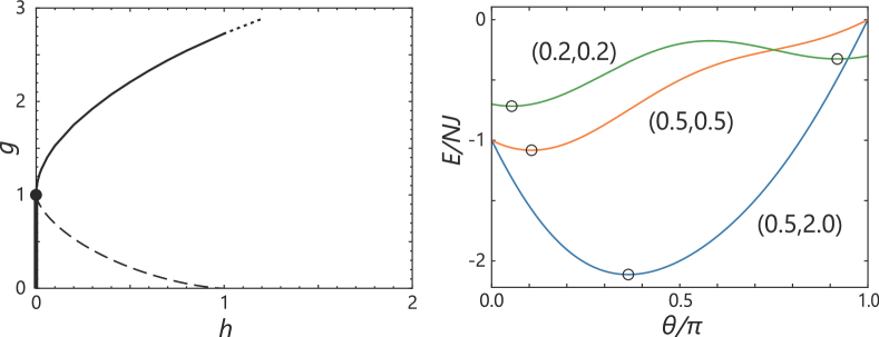
Figure 1: Left: Phase diagram of the quenched LMG model. The phase boundary is shown by the bold line and the critical point by the dot. The solid line obtained from a semiclassical analysis in Ref. [17] represents the boundary on the DQPTs. Below the sold line, we observe dynamical singularities of $f(t)$. The metastable state exists below the dashed line. Right: Equation (13) for several values of $(h,g)$. The circle marks denote local minimum points.

A possible behavior is roughly inferred from the equilibrium statistical properties of the Hamiltonian in the thermodynamic limit $N\to\infty$. We show the phase diagram in the left panel of Fig. 1. At the limit, the system is described semiclassically and the ground state is evaluated by parameterizing the spin as $\bm{S}=\frac{N}{2}(\sin\theta,0,\cos\theta)$ with $0\leq\theta\leq\pi$. The ground-state energy is written as $E_{\mathrm{gs}}=\min_{\theta}E(\theta)$ where

$$E(\theta)=-NJ\left(\frac{1}{2}\cos^{2}\theta+h\cos\theta+g\sin\theta\right).$$ (13)

We show the function for several values of $(h,g)$ in the right panel of Fig. 1. When the bias field $h$ is absent, $E(\theta)$ is minimized at $\theta=\pi/2$ at $g\geq 1$ and at $\theta=\arcsin g$ at $g\leq 1$. The latter has two possible solutions of $\theta$, showing the spin-reflection symmetry. The point $(h,g)=(0,1)$ is identified as the critical point. For nonzero values of $h$, $\arg\min_{\theta}E(\theta)$ uniquely exists and we observe no sharp transition.

When $h$ and $g$ are small enough, we observe a local minimum in addition to the global minimum. The local minimum represents the metastable state and exists when

$$g<(1-h^{2/3})^{3/2},$$ (14)

with $0<h<1$. The spinodal line representing the boundary is shown in the left panel of Fig. 1.

A semiclassical analysis of the survival amplitude was closely discussed in Ref. [17]. It was shown that the rate function $f(t)$ at $N\to\infty$ has singular points when $g$ is small. As a noteworthy result, the rate function at $g=0$ is obtained from the saddle-point analysis as

$$\lim_{N\to\infty}f(t)=\min_{n\in\mathbb{Z}}\frac{(hJt-\pi n)^{2}}{2[1+(Jt)^{2}]}.$$ (15)

We show typical behavior of the rate function in Fig. 2.

Thus, we conclude the phase diagram of the quenched LMG model in the left panel of Fig. 1. We note that our definition of the dynamical singularity is applied to the survival amplitude. The introduction of the symmetry-breaking $h$ implies that we do not observe singularities for the order parameter, the expectation value of $S^{z}$.

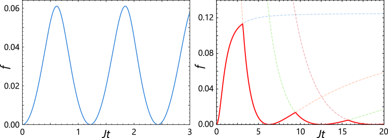
Figure 2: The rate function $f(t)$ for the quenched LMG model. The result on the left panel is obtained numerically with the parameters $(h,g)=(0.5,3.0)$ and $N=400$. The right panel represents Eq. (15) for $(h,g)=(0.5,0.0)$.

II.3 Representation in $S^{z}$-eigenstate basis

Although the $S^{x}$-eigenstate basis is convenient for the initial state, it is not for the Hamiltonian. We can switch to the $S^{z}$-eigenstate basis representation to write

$$\frac{H}{NJ} = -\sum_{k=0}^{N}\left[2\left(\frac{k}{N}-\frac{1+h}{2}\right)^{2}-\frac{h^{2}}{2}\right]|S-k\rangle_{z}{}_{z}\langle S-k|$$

$$-\sum_{k=0}^{N}g\sqrt{\frac{k}{N}\left(1-\frac{k}{N}\right)}$$

$$\times\left(|S-k+1\rangle_{z}{}_{z}\langle S-k|+|S-k\rangle_{z}{}_{z}\langle S-k+1|\right),$$

where we use the $S^{z}$ basis $|m\rangle_{z}$ with $m=\frac{N}{2}-k$. In the same basis, the initial state in Eq. (12) is written as

$$|\psi_{0}\rangle = \sum_{k=0}^{N}\left(\frac{1}{2}\right)^{N/2}\sqrt{\left(\begin{array}[]{c}N\\ k\end{array}\right)}|S-k\rangle_{z}$$

$$\sim \sum_{k=0}^{N}\left(\frac{2}{\pi N}\right)^{1/4}\exp\left[-N\left(\frac{k}{N}-\frac{1}{2}\right)^{2}\right]|S-k\rangle_{z}.$$

In the second line, we use the Stirling’s approximation which is justified at large $N$. Since the initial state is localized in the $x$-basis, it is extended in the $z$-basis. However, when we take the large-$N$ limit, the state is localized around the point $m=0$ with a width proportional to $\sqrt{N}$.

Thus, when we consider large values of $N$, we observe spreading of the zero-magnetization state to nonzero states. The first term of Eq. (LABEL:Hamz) plays the role of potential and the second term represents nearest-neighbor hopping. For large $g$, the hopping term is the dominant contribution. Since the hopping amplitude is maximum around the initial state, the state oscillates around the initial state. When $g$ takes a smaller value, the potential term enhances the spreading toward the positive-magnetization direction. When it reaches the state $k=0$, we observe a reflection, giving rise to a nontrivial interference of the wave function. We also see that the spreading toward the negative direction is more complicated. Although the increasing potential prevents the state from spreading, the potential produces a local minimum at $k=N$ when $h\leq 1$. It represents the metastable state and we expect a nontrivial behavior.

Thus, by using the $S^{z}$-eigenstate representation, we can develop a qualitative picture of the time evolution. To make the picture more quantitative, we apply the Krylov algorithm to our Hamiltonian.

III Dynamical quantum phase transitions

We numerically calculate the Krylov basis and the Lanczos coefficients. To reduce numerical errors, we use the full orthogonalization procedure [27] instead of using the three-term recurrence in Eq. (3). Then, by using the obtained Lanczos coefficients, we solve the time evolution in Eq. (7) to calculate the complexity $K(t)$ and the entropy $S(t)$. We also calculate the expectation values of $S^{z}$ and $S^{x}$ from the time evolution $|\psi(t)\rangle$ without the Krylov algorithm.

III.1 Lanczos coefficients

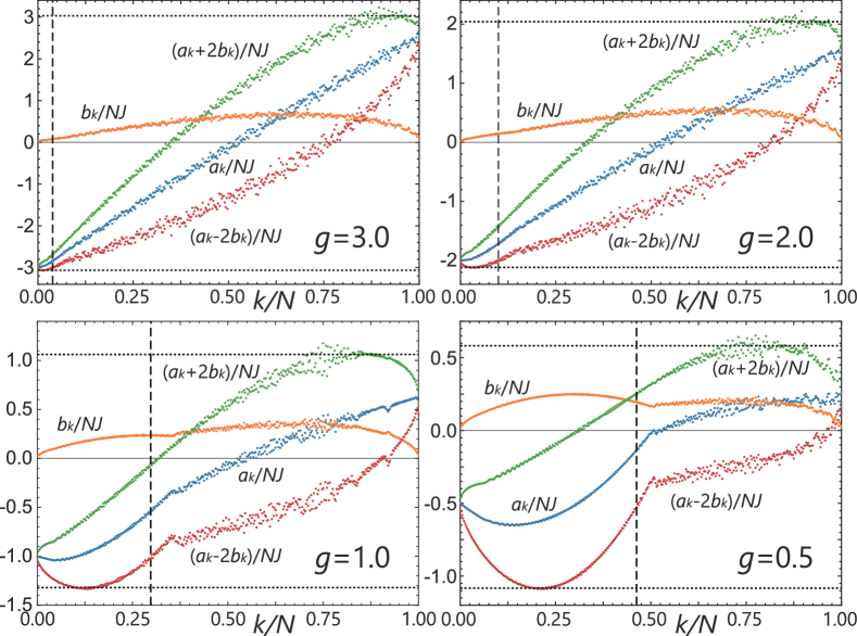
Figure 3: The Lanczos coefficients $a_{k}$ and $b_{k}$ for $N=400$, $h=0.5$, and $g=3.0,2.0,1.0,0.5$. The horizontal dotted lines in each panel represent the maximum and minimum eigenvalues of the Hamiltonian, in units of $NJ$. The vertical dashed line represents the maximum value of the complexity, $\max_{t}K(t)/N$. The complexity is shown in Fig. 5.

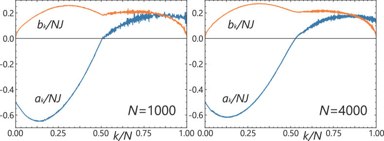
Figure 4: The size dependence of the Lanczos coefficients for $(h,g)=(0.5,0.5)$. We take $N=1000$ for the left panel and 4000 for the right.

In Fig. 3, we plot the Lanczos coefficients for the system size $N=400$. We fix $h=0.5$ and take several values for $g$. When $g$ is large enough and the state has no DQPT, $a_{k}$ grows almost linearly and $b_{k}$ has an inverted parabola-like form with the maximum around the middle of the index range. The slope of $a_{k}$ is large enough and the time-evolved state cannot go far from the initial state. This result is consistent with the picture developed in Sec. II.3.

When we take a smaller $g$, $a_{k}$ takes the minimum at $k\neq 0$. We also observe two-domain structures both in $a_{k}$ and $b_{k}$ and growings of the first domain for decreasing $g$. The slope of $a_{k}$ for small $k$ is understood from the analytic evaluation

$$a_{1}-a_{0}=2J\left(g-\frac{3}{2}\right)+O(N^{-1}).$$ (21)

The nonzero minimum point appears at $g<3/2$. The range width of $a_{k}$, $\max_{k}a_{k}-\min_{k}a_{k}$, becomes smaller as $g$ decreases and the time-evolved state can reach higher Krylov-basis states. As we see in Fig. 4, the two-domain structure is preserved for larger values of $N$. A similar structure was numerically observed in the same model with a time-dependent modulation in Ref. [28].

The asymptotic form at $N\to\infty$ is obtained by parametrizing the Hamiltonian by indices $x_{k}=k/N$ with $0\leq x_{k}\leq 1$. We can write

$$\frac{H}{NJ} \sim -\sum_{k=0}^{N}\left[x_{k}(1-x_{k})+g(1-2x_{k})\right]|S-k\rangle_{x}{}_{x}\langle S-k|$$

$$-\sum_{k=1}^{N}h\sqrt{x_{k}(1-x_{k})}$$

$$\times\left(|S-k+1\rangle_{x}{}_{x}\langle S-k|+|S-k\rangle_{x}{}_{x}\langle S-k+1|\right)$$

$$-\sum_{k=2}^{N}\frac{1}{2}x_{k}(1-x_{k})$$

$$\times\left(|S-k+2\rangle_{x}{}_{x}\langle S-k|+|S-k\rangle_{x}{}_{x}\langle S-k+2|\right).$$

When $a_{k}$ and $b_{k}$ change smoothly as functions of the index $k$, we can introduce the continuum representation as $(a_{k},b_{k})\to(a(x_{k}),b(x_{k}))$ at $N\to\infty$. The density of state for the Hamiltonian is written as [29]

$$\frac{\mathrm{Tr}\,\delta(E-H)}{\mathrm{Tr}\,1}\sim\int_{0}^{1}\frac{dx}{\pi}\,\frac{\Theta(4b^{2}(x)-(E-a(x))^{2})}{\sqrt{4b^{2}(x)-(E-a(x))^{2}}},$$ (23)

where $\Theta$ represents the step function. This representation denotes that the eigenvalues distribute in the range $[\min_{k}(a_{k}-2b_{k}),\max_{k}(a_{k}+2b_{k})]$. The result in Fig. 3 supports this property. We discuss in the previous section that $a_{k}$ corresponds to the local potential. To put it more accurately, subtracting the contribution from the kinetic energy, we can identify $a_{k}-2b_{k}$ as the local potential.

In Fig. 3, we also denote the maximum value of the complexity to be discussed in the following. As we see in the figure, the maximum value can be estimated from the local potential $a_{k}-2b_{k}$. The state is confined in a potential well and oscillates between $k=0$ and $k=\max_{t}K(t)$ where $a_{k}-2b_{k}$ takes an identical value.

III.2 Complexity and entropy

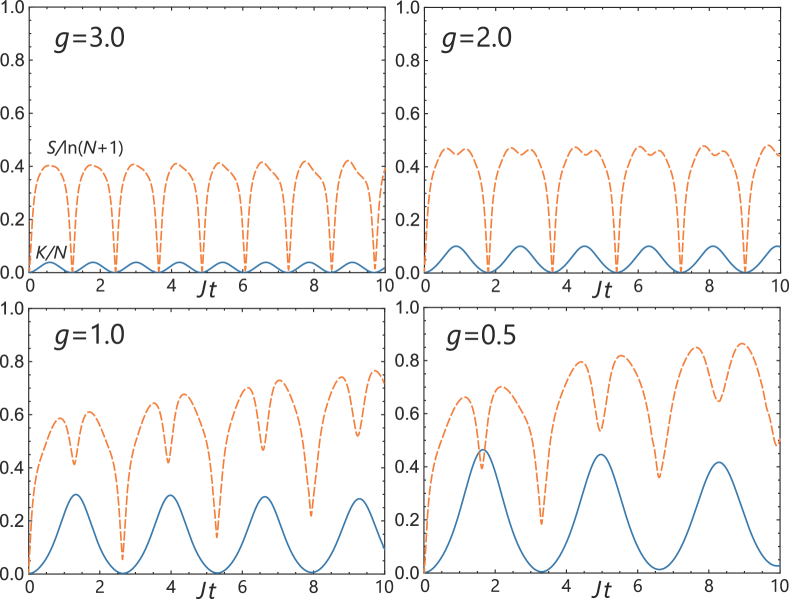
Figure 5: The complexity $K(t)$ (blue solid lines) and the entropy $S(t)$ (red dashed lines) for $N=400$, $h=0.5$, and $g=3.0,2.0,1.0,0.5$. For $g\leq g_{c}\sim 2.0$, the dynamical singularities of the rate function in Eq. (2) are obtained at the peak points of $K(t)$.

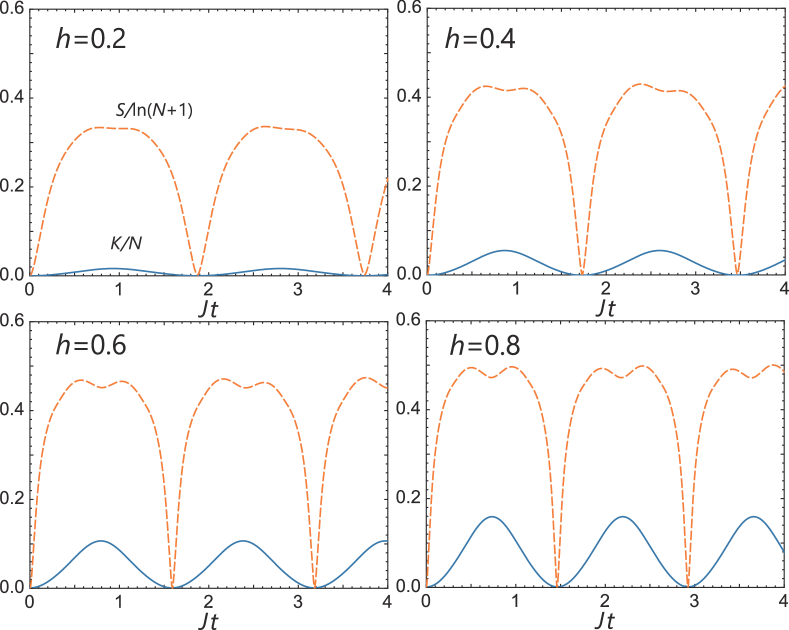
Figure 6: The complexity $K(t)$ (blue solid lines) and the entropy $S(t)$ (red dashed lines) for $N=400$, $g=2.2$, and $h=0.2,0.4,0.6,0.8$. The dynamical singularities are obtained when $h\geq h_{c}\sim 0.5$.

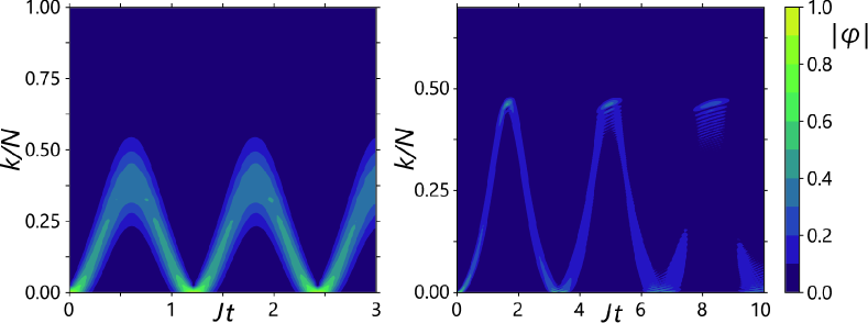
Figure 7: Distributions of $|\varphi_{k}(t)|$. We take $(h,g)=(0.5,3.0)$ for the left panel and $(0.5,0.5)$ for the right. The system size is $N=400$.

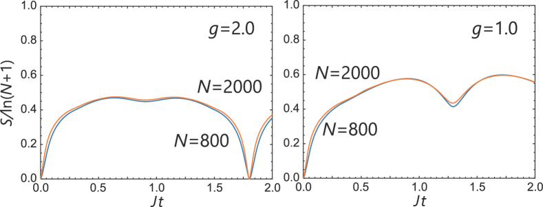
Figure 8: The entropy $S(t)$ for $N=800$ and $2000$. We take $(h,g)=(0.5,2.0)$ for the left panel and $(0.5,1.0)$ for the right.

As we see in Fig. 3, the Lanczos coefficients with large indices are unstable and we observe small oscillations. However, the unstable fluctuations do not affect the actual time evolution because the state spreading is basically restricted to lower indices. We show the complexity $K(t)$ in Figs. 5 and 6. The height of the first peak represents the maximum value of $K(t)$ and is denoted in Fig. 3. As we see in Fig. 7, the distribution of the complexity is a single-peaked function at large $g$. When $g$ is small, the complexity has broad distributions as $t$ grows. The result is sensitive to the choice of the system size, and it is difficult to know the exact long-time behavior. In the next section, we study some more details on the distributions of the complexity.

When $g$ is small, the dynamical singularities of the rate function in Eq. (2) appear at the peak points of $K(t)$. It means that the DQPT is obtained when the state is reflected by the potential at far-reaching points. We however find that the complexity does not exhibit any singular behavior. This is because the complexity is given by the sum of many components of $\varphi_{k}$, while the survival probability is obtained only from the zeroth component. Furthermore, we need take the logarithm of the survival probability, as Eq. (2), to find the singularity.

We also plot the entropy $S(t)$ in Figs. 5 and 6. When $g$ is large enough and no DQPT is observed, $S(t)$ shows a similar oscillation as $K(t)$. The entropy representing an uncertainty of the state is maximized when the state reaches a reflection point. This behavior is changed when $g$ is small. We observe small dips at the DQPT points. As we see in Fig. 8, no singular behavior is obtained up to considerably large values of $N$. Since the zeroth-component contribution $-|\varphi_{0}(t)|^{2}\ln|\varphi_{0}(t)|^{2}$ to $S(t)$ is exponentially small in $N$ and is negligible, this nonsingular result is reasonable. Our result shows that the DQPT involves a structural change of the entropy.

III.3 Average of spin operators

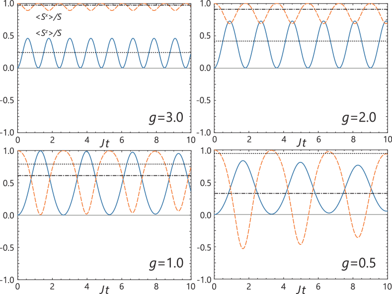
Figure 9: The expectation values of spin operators $S^{z}$ (blue solid lines) and $S^{x}$ (red dashed lines) for $N=400$, $h=0.5$, and $g=3.0,2.0,1.0,0.5$. The dotted line in each panel represents the equilibrium value of $S^{z}$ at the ground state, and the dot-dashed line represents the value of $S^{x}$.

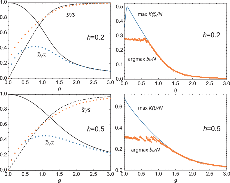
Figure 10: Left: The time-averaged expectation values of $S^{z}$ (blue dots) and $S^{x}$ (red dots). We take $h=0.2$ for the upper panel and $h=0.5$ for the lower panel. The system size is $N=400$. The time average is taken over the range $0\leq Jt\leq 100$. The dashed line represents the equilibrium value of $S^{z}$ at the ground state, and the dotted line represents the value of $S^{x}$. Right: $\max_{t}K(t)$ (blue solid line) and $\mathrm{argmax}_{k\leq\max_{t}K(t)}\,b_{k}$ (red dots).

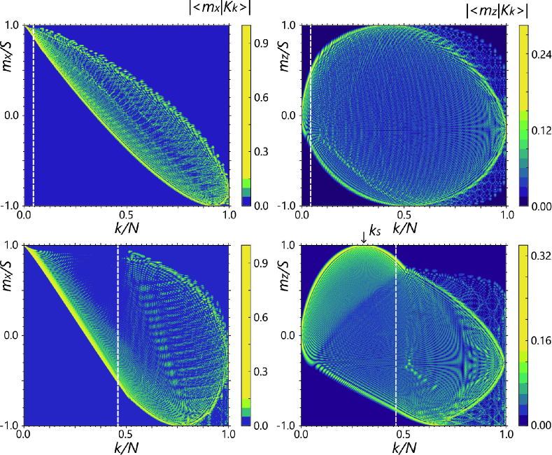
Figure 11: The left panels show $|{}_{x}\langle m_{x}|K_{k}\rangle|$ and the right panels $|{}_{z}\langle m_{z}|K_{k}\rangle|$. We take $(h,g)=(0.5,3.0)$ for the upper panels and $(h,g)=(0.5,0.5)$ for the lower panels. The system size is $N=400$. The white dashed lines denote the maximum value of the complexity taken from Fig. 5. See text for $k_{S}$.

The DQPT for the survival probability can be distinguished from that for the order parameter [30, 20]. In the present study, we apply the longitudinal field $h$ that breaks spin-reflection symmetry. As a result, it is expected that no sharp transition is observed for the magnetization. We calculate the expectation values of the spin operators $S^{z}$ and $S^{x}$ at each time and the result is plotted in Fig. 9. We observe regular oscillations at large $g$ and decaying oscillations at small $g$. The oscillation period coincides with that of $K(t)$. The expectation value $\langle\psi(t)|S^{z}|\psi(t)\rangle$ is locally-maximized at the DQPT points and $\langle\psi(t)|S^{x}|\psi(t)\rangle$ is locally-minimized.

We also plot in Fig. 9 the expectations with respect to the ground state of the Hamiltonian. We find that each time average of $\langle\psi(t)|S^{z,x}|\psi(t)\rangle$ is close to the corresponding ground-state expectation at large $g$, and deviates from that at small $g$. In the left panels of Fig. 10, we compare each of the time averages $\overline{S}^{z,x}=\int_{0}^{t}ds\,\langle\psi(s)|S^{z,x}|\psi(s)\rangle/t$ for a large $t$ to the ground-state expectation. We see that they are close with each other at large $g$ and deviate significantly at small $g$. The deviation starts around the DQPT point but the change is smooth as a function of $g$. At small $g$, we observe a peak of $\overline{S}^{z}$, which is contrasted to the monotonic change of the ground-state expectation. We find that this peak is related to the similar structure of $b_{k}$ in Fig. 3. In the range $0<k\leq\max_{t}K(t)$, $b_{k}$ for a small $g$ has a peak at an intermediate value and the appearance of the peak corresponds to the nonmonotonic behavior of $\overline{S}^{z}$, as we show in the right panel of Fig. 10.

Although the dynamical properties of the system can be understood only from the Lanczos coefficients, it is instructive to see the Krylov basis $|K_{k}\rangle$. The left panels of Fig. 11 show $|{}_{x}\langle m_{x}|K_{k}\rangle|$. The initial state $|K_{0}\rangle$ is localized at $m_{x}=S$ and $|K_{k}\rangle$ involves smaller $m_{x}$ contributions as we increase $k$. The spreading is almost linear and the basis state reaches $m_{x}=-S$ at some point smaller than $k=N$. Since the original Hamiltonian involves the next-nearest-neighbor hopping in the $x$-basis, it is naively expected that the basis state reaches the minimum point $m_{x}=-S$ at $k=N/2$. However, the spreading is disturbed by the presence of the other contributions. We note that the spreading is maximized only when there are no other contributions [28].

The $S^{z}$-eigenstate-basis distribution of $|K_{k}\rangle$ in the right panels of Fig. 11 shows a more complicated behavior. The initial state in the $z$-basis is written as Eq. (LABEL:psi0z). Applying the Krylov expansion, we see that the distribution spreads over both the positive and negative directions. The spreading in the positive direction is faster that that in the negative direction. The spreading front of the former reaches the maximum value $m_{z}=S$ at a point $k=k_{S}$. We display the location of $k_{S}$ in Fig. 11. This value of $k_{S}$ represents the peak of $b_{k}$ in the first domain of the two-block structure. The decreasing of $b_{k}$ at $k>k_{S}$ in the first domain is interpreted as a saturation of the state basis. As a result, we observe a nonmonotonic behavior of $\overline{S}^{z}$ in Fig 10.

IV Metastable state

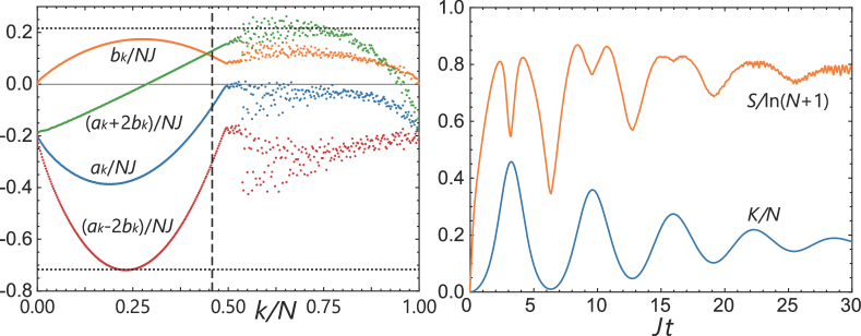
Figure 12: The left panel shows the Lanczos coefficients, and the right panel shows the complexity and the entropy. We take $N=400$ and $(h,g)=(0.2,0.2)$.

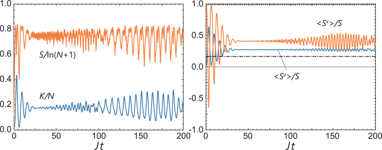
Figure 13: Long-time behavior of the complexity, the entropy, and the spin expectations for $N=200$ and $(h,g)=(0.2,0.2)$.

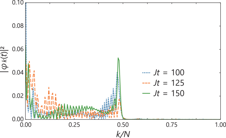
Figure 14: Probability distributions in Krylov space at large $t$. We take $N=200$ and $(h,g)=(0.2,0.2)$.

The two-block structure of the Lanczos coefficients appears in a wide range of small $g$. We study the parameter range where the metastable state exists and the result at $(h,g)=(0.2,0.2)$ is shown in Figs. 12, 13, and 14.

In the left panel of Fig. 12, we observe a decreasing of $a_{k}$ in the second block at large $k$ giving rise to local minimum points. Since $a_{k}-2b_{k}$ is interpreted as a local potential, the emergence of the local minimum implies the presence of a metastable state. As we see in the right panel of Fig. 12, the complexity is still an oscillating function and the DQPTs are found at local maximum points. Correspondingly, the entropy gives dips as we discuss in the previous section.

Since the DQPT is obtained at large $N$, it must be independent of the presence of the metastable state. Generally, the metastable states affect the behavior at long times. In Fig. 13, we show the complexity, the entropy, and the spin expectations for a smaller value of $N$. They show unstable oscillations at large $t$, which are not observed in the absence of the metastable state. In Fig. 14, we plot distributions of the complexity at several large values of $t$. The complexity has a broad distribution and the probability for the state to reach the second domain takes a small nonzero value.

V Dimensionality reduction

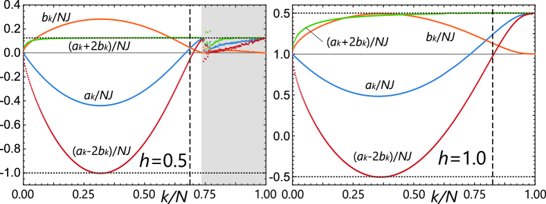
Figure 15: The Lanczos coefficients for $N=400$, $g=0$, $h=0.5$ (left panel) and $h=1.0$ (right). In the left panel, $b_{k}$ takes a small value at some point $d$ with $d<N$ and the shaded domain is discarded.

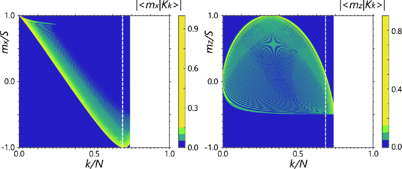
Figure 16: The spin-eigenstate distributions of the Krylov basis. We take $N=400$ and $(h,g)=(0.5,0.0)$. The white dashed lines denote the maximum value of the complexity.

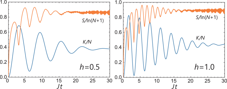
Figure 17: The left panel shows the complexity $K(t)$ and the entropy $S(t)$ at $(h,g)=(0.5,0.0)$, and the right panel show those at $(h,g)=(1.0,0.0)$. We take $N=400$.

We discuss the special case at $g=0$ where the Hamiltonian only involves the $S^{z}$ operator. In the $z$-basis representation, each of the components evolves independently from the initial Gaussian distribution in Eq. (LABEL:psi0z).

We show the result at $g=0$ in Figs. 15, 16, and 17. As we see in Fig. 15, when $h$ is small, $b_{k}$ takes a very small value at a point smaller than $N$. This implies that the Krylov dimension is smaller than the Hilbert space dimension. In principle, the Krylov algorithm halts when we have $b_{k}=0$. However, numerical calculations never give the exact value of zero and we obtain artificial sequences of the Lanczos coefficients until $k=N$. The Krylov dimension is roughly estimated as

$$d(h)\sim\min\left(\frac{1+h}{2}N,N\right).$$ (24)

Figure 16 represents the distributions of $|K_{k}\rangle$ with respect to the spin-eigenstate basis $|m_{x}\rangle_{x}$ and $|m_{z}\rangle_{z}$. The spreading in $x$-basis space is almost linear and the basis vector reaches the eigenstate $m_{x}=-S$. On the other hand, in the $z$-basis case, the spreading in the negative direction is suppressed significantly, which is consistent with the reduction of the Krylov dimension.

The absence of the second block in the Lanczos coefficients implies that the effect of the metastable state is negligible. We do not observe unstable large fluctuations in Fig. 17. This is due to the simple form of the Hamiltonian. In the case of $g=0$, the Hamiltonian only contains the $S^{z}$ operator and tunneling effects due to quantum fluctuations are absent.

VI Conclusions

We have discussed real-time evolutions of quantum states for the fully-connected spin model. Applying the Krylov algorithm, we find that quenched dynamics is described by the spreading in Krylov space. The dynamical singularities can occur when the state is reflected from a potential barrier in Krylov space.

Although we cannot identify the DQPT from the complexity, the DQPT involves a structural change of the entropy. We also find that by knowing the structure of the Lanczos coefficients, we can predict many dynamical properties of the system without calculating the time evolution, such as the maximum value of the complexity, the existence of metastable states, and the nonmonotonic behavior of the order parameter.

One of the most important advantages of the Krylov subspace method is that the system is mapped onto a one-dimensional system. This mapping enables quenched dynamics for various quantum systems to be studied in a unified manner. The differences in behaviors can be best seen in the response to quenching involving large parameter changes, where distinct spreading patterns in Krylov space emerge.

Our findings suggest that the Krylov subspace approach provides a powerful framework for understanding quantum dynamics beyond conventional methods. This perspective not only offers computational advantages but also provides deeper physical insights into DQPTs and non-equilibrium phenomena. Future work could extend this approach to more complex systems and explore connections between the Krylov space structure and other quantum information metrics.

References

- Calabrese and Cardy [2006] P. Calabrese and J. Cardy, Time dependence of correlation functions following a quantum quench, Phys. Rev. Lett. 96, 136801 (2006).
- Polkovnikov et al. [2011] A. Polkovnikov, K. Sengupta, A. Silva, and M. Vengalattore, Colloquium: Nonequilibrium dynamics of closed interacting quantum systems, Rev. Mod. Phys. 83, 863 (2011).
- Eisert et al. [2015] J. Eisert, M. Friesdorf, and C. Gogolin, Quantum many-body systems out of equilibrium, Nature Phys. 11, 124 (2015).
- Mitra [2018] A. Mitra, Quantum quench dynamics, Annual Review of Condensed Matter Physics 9, 245 (2018).
- Heyl et al. [2013] M. Heyl, A. Polkovnikov, and S. Kehrein, Dynamical quantum phase transitions in the transverse-field ising model, Phys. Rev. Lett. 110, 135704 (2013).
- Heyl [2014] M. Heyl, Dynamical quantum phase transitions in systems with broken-symmetry phases, Phys. Rev. Lett. 113, 205701 (2014).
- Heyl [2015] M. Heyl, Scaling and universality at dynamical quantum phase transitions, Phys. Rev. Lett. 115, 140602 (2015).
- Jurcevic et al. [2017] P. Jurcevic, H. Shen, P. Hauke, C. Maier, T. Brydges, C. Hempel, B. P. Lanyon, M. Heyl, R. Blatt, and C. F. Roos, Direct observation of dynamical quantum phase transitions in an interacting many-body system, Phys. Rev. Lett. 119, 080501 (2017).
- Heyl [2018] M. Heyl, Dynamical quantum phase transitions: a review, Reports on Progress in Physics 81, 054001 (2018).
- Viswanath and Müller [1994] V. Viswanath and G. Müller, The Recursion Method: Application to Many-Body Dynamics (Springer-Verlag, 1994).
- Nandy et al. [2024] P. Nandy, A. S. Matsoukas-Roubeas, P. Martínez-Azcona, A. Dymarsky, and A. del Campo, Quantum dynamics in krylov space: Methods and applications (2024), arXiv:2405.09628 [quant-ph] .
- Parker et al. [2019] D. E. Parker, X. Cao, A. Avdoshkin, T. Scaffidi, and E. Altman, A universal operator growth hypothesis, Phys. Rev. X 9, 041017 (2019).
- Caputa et al. [2022] P. Caputa, J. M. Magan, and D. Patramanis, Geometry of krylov complexity, Phys. Rev. Res. 4, 013041 (2022).
- Balasubramanian et al. [2022] V. Balasubramanian, P. Caputa, J. M. Magan, and Q. Wu, Quantum chaos and the complexity of spread of states, Phys. Rev. D 106, 046007 (2022).
- Lipkin et al. [1965] H. Lipkin, N. Meshkov, and A. Glick, Validity of many-body approximation methods for a solvable model: (i). exact solutions and perturbation theory, Nuclear Physics 62, 188 (1965).
- Žunkovič et al. [2016] B. Žunkovič, A. Silva, and M. Fabrizio, Dynamical phase transitions and loschmidt echo in the infinite-range xy model, Philosophical Transactions of the Royal Society A: Mathematical, Physical and Engineering Sciences 374, 20150160 (2016), https://royalsocietypublishing.org/doi/pdf/10.1098/rsta.2015.0160 .
- Obuchi et al. [2017] T. Obuchi, S. Suzuki, and K. Takahashi, Complex semiclassical analysis of the loschmidt amplitude and dynamical quantum phase transitions, Phys. Rev. B 95, 174305 (2017).
- Bhattacharjee et al. [2022] B. Bhattacharjee, X. Cao, P. Nandy, and T. Pathak, Krylov complexity in saddle-dominated scrambling, Journal of High Energy Physics 2022, 10.1007/jhep05(2022)174 (2022).
- Afrasiar et al. [2023] M. Afrasiar, J. K. Basak, B. Dey, K. Pal, and K. Pal, Time evolution of spread complexity in quenched lipkin–meshkov–glick model, Journal of Statistical Mechanics: Theory and Experiment 2023, 103101 (2023).
- Bento et al. [2024] P. H. S. Bento, A. del Campo, and L. C. Céleri, Krylov complexity and dynamical phase transition in the quenched lipkin-meshkov-glick model, Phys. Rev. B 109, 224304 (2024).
- Pal et al. [2023] K. Pal, K. Pal, and T. Sarkar, Complexity in the lipkin-meshkov-glick model, Phys. Rev. E 107, 044130 (2023).
- Bhattacharya et al. [2024] A. Bhattacharya, P. P. Nath, and H. Sahu, Krylov complexity for nonlocal spin chains, Phys. Rev. D 109, 066010 (2024).
- Guerra et al. [2025] E. M. Guerra, I. Gornyi, and Y. Gefen, Correlations and krylov spread for a non-hermitian hamiltonian: Ising chain with a complex-valued transverse magnetic field (2025), arXiv:2502.07775 [quant-ph] .
- Shirokov et al. [2025] I. Shirokov, V. Hrushev, F. Uskov, I. Dudinets, I. Ermakov, and O. Lychkovskiy, Quench dynamics via recursion method and dynamical quantum phase transitions (2025), arXiv:2503.24362 [cond-mat.str-el] .
- Barbón et al. [2019] J. Barbón, E. Rabinovici, R. Shir, and R. Sinha, On the evolution of operator complexity beyond scrambling, Journal of High Energy Physics 2019, 10.1007/jhep10(2019)264 (2019).
- Fan [2022] Z.-Y. Fan, Universal relation for operator complexity, Phys. Rev. A 105, 062210 (2022).
- Rabinovici et al. [2021] E. Rabinovici, A. Sánchez-Garrido, R. Shir, and J. Sonner, Operator complexity: a journey to the edge of krylov space, Journal of High Energy Physics 2021, 62 (2021).
- Takahashi and del Campo [2025] K. Takahashi and A. del Campo, Krylov subspace methods for quantum dynamics with time-dependent generators, Phys. Rev. Lett. 134, 030401 (2025).
- Balasubramanian et al. [2023] V. Balasubramanian, J. M. Magan, and Q. Wu, Tridiagonalizing random matrices, Phys. Rev. D 107, 126001 (2023).
- Marino et al. [2022] J. Marino, M. Eckstein, M. S. Foster, and A. M. Rey, Dynamical phase transitions in the collisionless pre-thermal states of isolated quantum systems: theory and experiments, Reports on Progress in Physics 85, 116001 (2022).