Vortex droplets and lattice patterns in two-dimensional traps: A photonic spin-orbit-coupling perspective
Abstract
In the context of the mean-field exciton-polariton (EP) theory with balanced loss and pump, we investigate the formation of lattice structures built of individual vortex-antivortex (VAV) bound states under the action of the two-dimensional harmonic-oscillator (HO) potential trap and effective spin-orbit coupling (SOC), produced by the TE-TM splitting in the polariton system. The number of VAV elements (“pixels”) building the structures grow with the increase of self- and cross-interaction coefficients. Depending upon their values and the trapping frequency, stable ring-shaped, circular, square-shaped, rectangular, pentagonal, hexagonal, and triangular patterns are produced, with the central site left vacant or occupied in the lattice patterns of different types. The results suggest the experimental creation of the new patterns and their possible use for the design of integrated circuits in EP setups, controlled by the strengths of the TE-TM splitting, nonlinearity, and HO trap.
I Introduction
Systems of interacting quantum fluids offer broad opportunities for investigating various macroscopic quantum phenomena, such as supersolidity [1, 2, 3], vorticity [4, 5, 6], quantum droplets (QDs) [7, 8, 9], and others. In particular, the studies of QDs gained impetus in low-temperature physics due to the possibility of their experimental observation in Bose-Einstein condensates (BECs) [10, 11]. Recently, much interest has been drawn to this subject due to the forecast [12, 13] and synthesis of ultra-diluted QDs in binary homonuclear [14, 15] and heteronuclear [16, 17] Bose-Einstein condensates, where they are sustained by the stable equilibrium between the contact (short-range) mean-field interactions and the corrections to them, induced by quantum fluctuations. The QD stability relies on the equilibrium between the surface tension and bulk energy of the droplets. In addition to the creation of stable QDs, their collisions in 1D [18], 2D [19], and 3D [20] geometries have also been studied (experimentally, in the latter case), as well as scattering of 1D QDs on localized potentials [21].
In addition to BECs with contact interactions, the bosonic condensates of magnetic atoms with long-range dipolar interactions provide the setting for the creation of stable anisotropic QDs and lattice patterns built of them [22, 23, 24, 25, 26, 27, 28], including, in particular, a nearly spatially periodic stripe-shaped one, known as the superstripe state, which is maintained by the 3D harmonic-oscillator (HO) trapping potential [29]. These Spatially structured configurations may represent ground states and metastable ones. Further, stable 2D [30, 31, 32] and 3D [33] vortex QDs with embedded angular momentum have been predicted too; see a brief review in Ref. [34]. On the other hand, vortex QDs in dipolar BEC were found to be unstable [35]. The stability of 3D vortex QDs can also be provided by a toroidal trapping potential [36]. A similar mechanism secures the stabilization of 2D vortex QDs with multiple vorticity [37, 38] and multipole 2D QDs [39]. Furthermore, the stability of the droplets can be assessed through modulation instability [40, 41]. Recently [42] examined the modulation instability of BEC in presence of impurities. QDs were explored too in binary condensates with spin-orbit coupling (SOC) [43, 44, 45, 46]. Generally, the interplay of SOC with the intrinsic nonlinearity makes it possible to create various lattice-shaped and localized patterns in binary BEC [47, 48, 49, 50, 51]. Recent studies have also explored the existence and stability of vortex solitons under the joint action of SOC and Rydberg interactions [52, 53]. Parallel to the studies of this phenomenology in BEC, SOC effects have also been explored in photonics. Specifically, stable two-dimensional matter-wave solitons sustained by SOC in binary BEC in the form of semi-vortices and mixed modes [48], can be emulated by spatiotemporal propagation of light in a dual-core nonlinear optical waveguide, where the effective SOC is characterized by the temporal dispersion of the inter-core coupling [54].
In the realm of photonics, SOC effects play a significant role in exciton-polariton (EP) condensates in semiconductor microcavities [55, 56, 57, 58, 59]. Polaritons are hybrid modes which couple a material component, represented by excitons in quantum wells and cavity photons. They are represented by a two-component pseudospinor wave function. In contrast to atomic BECs, the dynamics of EP condensates are nonconservative, owing to significant material and defect-induced losses in the cavities. The advantage of employing EP condensates as macroscopic (classical) simulators of the SOC phenomena in quantum matter lies in the ease of identifying polariton states through emitted light in the host microcavity. The polarization of photons in microcavities at oblique angles gives rise to different transmission and reflection regimes, unlike the case of the normal incidence [60, 61, 62]. This phenomenon leads to the splitting of transverse-electric and magnetic (TE and TM) modes, which play a fundamental role in the realization of the photonic SOC; it also promotes the distribution of spin-polarized polaritons and causes periodic oscillations of the photonic pseudospin [63]. The effect of the polarization structure of photons on EP states give rise to a profound nonlinearity that facilitates the emergence of self-sustained nonlinear topological modes, such as half-vortices [64, 65], topological polaritons [61], and skyrmions [66]. The nonlinearity may also be used for the development of applications [67, 68]. Recent experiments confirmed the generation of vortices in EP condensates [69], utilizing a cylindrically asymmetric in-plane optical trap imposed by a composite nonresonant excitation beam. Furthermore, the creation of half-vortices through the interaction of the TE-TM and Zeeman splittings under the action of the ring-shaped potential, produced by an external nonresonant depolarized pump has been demonstrated in Ref. [70]. While the actual confinement in polariton condensates is provided by Bragg reflectors and detuning effects, rather than an external HO trap, it may be used as an effective confinement model [71]. In this context, the TE-TM splitting affects the stability of half-vortices in the conservative setting [72, 73], as well as in the presence of loss and gain [74]. Accordingly, the half-vortex profiles are “warped” by the TE-TM splitting, losing their axial symmetry [75]. The recent analysis of the modulation instability under the action of the photonic SOC [76] reveals the emergence of wave modes and opens ways for exploring novel nonlinear phenomena in EP condensates that incorporate the TE-TM splitting and magnetic fields, such as the condensate-reservoir regime [77] and multimode dynamics [78]. In addition to this, the inclusion of the Raman effect is likely to enhance instability phenomena in the dynamics of EP condensates [79].
EP interaction systems may be used in various applications, such as quantum-information processing, where polaritons can be manipulated to design quantum gates [80], and EP-based lasers, that may operate more efficiently than usual lasers [81].
The objective of the present work is to study the dynamics of EP condensates in the context of an effectively 2D conservative system, specifically focusing on SOC induced by the TE-TM splitting. In the two-component (spinor) system of Gross-Pitaevskii (GP) equations, which model the EP condensate, SOC is represented by the second-order differential operator, unlike the first-order operator which represents SOC in BEC of ultracold atomic gases. Due to this fact, the GP system for the EP condensates gives rise to two-component bound states of the vortex-antivortex (VAV) type [55], in addition to semi-vortices (SVs), that exist as stable states in the case of the first-order SOC operator [48]. In this work, we demonstrate that multiple VAV elements (“pixels”) can build stable circular, hexagonal, triangular, and pentagonal lattice configurations. We address the settings which include the HO trapping potential acting in the 2D plane , while it is implied that the reduction of the original 3D system to its 2D form is provided by the action of the tight confinement in the transverse direction. The stability of the VAV bound state and various lattice patterns built of VAV pixels are established by dint of numerical simulations of the long-time evolution.
The paper is organized as follows. In Section II, we present the nonlinear mean-field (GP) model for the EP condensate under the action of the TE-TM splitting and 2D trapping potential. In Section III, we present systematically generated numerical findings for various lattice configurations. The paper is concluded in Section IV.
II The model
EP condensates trapped in microcavities are quantum fluids that exhibit nonlinear dynamical properties. Unlike atomic BECs, polaritons are inherently dissipative modes whose dynamics are affected by the balance between the gain, which is provided by a reservoir, and loss, determined by a finite EP lifetime. The dynamics of the interacting EP condensates, confined by the 2D HO potential,
| (1) |
in the presence of the TE-TM splitting is modeled by the coupled GP equations for components of the EP spinor wave function [64, 58, 76]:
| (2a) | |||
| (2b) | |||
Here components and represent different polariton polarizations [82]. denotes 2D Laplacian, the normalized trapping frequency in Eq. (1) is , where is the frequency value in Hz, while is the frequency accounting for the strong transverse confinement, and represents the strength of the effective photonic SOC, i.e., the effect of the TE-TM splitting on the EP modes [58], [83]. As mentioned above, the TE-TM splitting in EP systems leads to anisotropic dispersion and spin-dependent coupling, enriching the system’s dynamics and allowing exploration of spin-textured patterns and polarization vortices. Further, is the intracomponent interaction coefficient, and
| (3) |
where is the coefficient accounting for the inter-component interactions. We here address the physically relevant case of and , which implies the repulsion and attraction of EPs with identical and opposite spins, respectively. The repulsive and attractive interactions in the EP system may be nearly canceled by means of the Feshbach resonance [84], which leads to .
The rate equations for reservoir densities , coupled to the GP system are written as
| (4) |
In this connection, the terms in Eq. (2) proportional to and represent the cumulative effects of the incoherent pump [whose rate is represented by term in Eq. (4)] and losses, with being the rate of scattering of excitons from the reservoir density into the condensate, while is the polariton decay rate. A crucial condition is that the excitonic reservoir density reaches a steady-state value, at which the reservoir pump () exactly compensates the decay rate [85]. We focus the study on the regime in which the EP-EP interaction, determined by factor ), dominates over the reservoir interaction (, ). Thus, the mutually compensated pump and loss terms may be neglected, and the condensate evolution is governed by the remaining nonlinear and SOC terms, effectively mimicking the conservative system [55]. In this case, Eqs. (2) simplify to
| (5a) | |||
| (5b) | |||
The scaled form of the conservative GP equations (5) uses units for lengths, time, energy, and density () defined, respectively, as , , , .
III Numerical results
Following Ref. [48], it is convenient to rewrite the 2D equations (5) in the polar coordinates, , with the linear SOC operators expressed by means of the identity
| (6) |
Stationary solutions to Eq. (5), with chemical potential , are sought in the conventional form.
| (7) |
where are integer vorticities, which are related by equality
 \SetHorizontalCoffin\labelcoffin
\SetVerticalPole\imagecoffinleft3pt+\CoffinWidth\labelcoffin/2\SetVerticalPole\imagecoffinright\Width-3pt-\CoffinWidth\labelcoffin/2\SetHorizontalPole\imagecoffinup\Height-3pt-\CoffinHeight\labelcoffin/2\SetHorizontalPole\imagecoffindown3pt+\CoffinHeight\labelcoffin/2\JoinCoffins\imagecoffin[left,up]\labelcoffin[vc,hc]\TypesetCoffin\imagecoffin
| (8) |
pursuant to the above-mentioned fact that the SOC terms are represented by the second-order operator in Eqs. (5). The substitution of ansatz (7) and potential (1) in Eqs. (5) gives rise to the radial equations for real stationary wave functions :
| (9) | |||||
Most fundamental solutions admitted by relation (8) represent VAV states, with
| (11) |
and SV ones, with
| (12) |
We here focus on the VAV state (11), as it has the best chances to be stable [55]. For this solution, with , Eqs. (9) and (III) reduce to the single radial equation:
| (13) | |||||
We initially discuss the linear system by setting . In this case, the exact solution to Eq. (13) amounts to the commonly known 2D HO wave function,
| (14) |
with the respective eigenvalue of the chemical potential,
| (15) |
Here, is an arbitrary amplitude, and this solution exists in the case of (including all values of ). Considering the nonlinear term in Eq. (13) as a perturbation, the first-order correction to the chemical potential is produced by the straightforward application of the quantum-mechanical perturbation theory to this equation:
| (16) |
where expression (3) is substituted for . The corresponding bound states are characterized by the normalized number of particles (norm),
| (17) |
which is a dynamical invariant of the system.
The mean-field equations (2) were solved numerically. Usually, the split-step Fourier-transform method [86, 87, 88], the Cranck-Nicolson one [89], and the pseudo-spectral method [90] are employed to produce numerical solutions. We here used the split-step algorithm, presenting the results in a normalized form. For the formation of VAV bound states, we fix realistic values of the parameters, viz., the SOC strength [55] trapping frequency Hz, and the transverse one Hz. The results also depend on the interaction coefficients, which are determined by the scattering length of atomic collisions and norm Eq. (17) loaded into the HO trap. Thus, numerical solutions for VAV bound states were obtained by solving Eq. (5) in real time, with respective initial states. For instance, to produce a square VAV lattice, the initial states should be of the same type. The stability is possible as a result of the interplay of the confinement imposed by the holding potential and repulsive interaction between the VAV pixels. The vortices of the same sign, with either or , repel each other in each component. The repulsive pairwise interactions between the pixels are an obvious stabilizing factor for multi-pixel patterns.
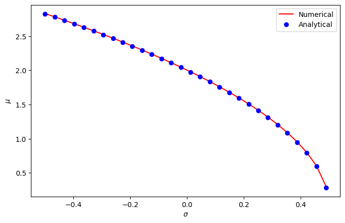
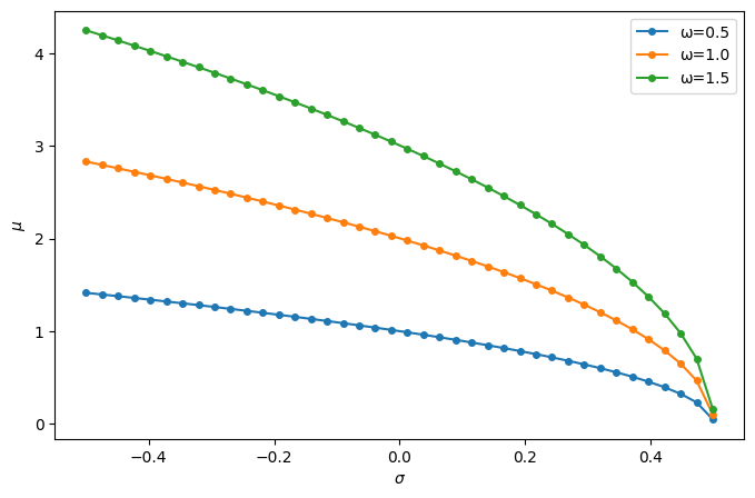
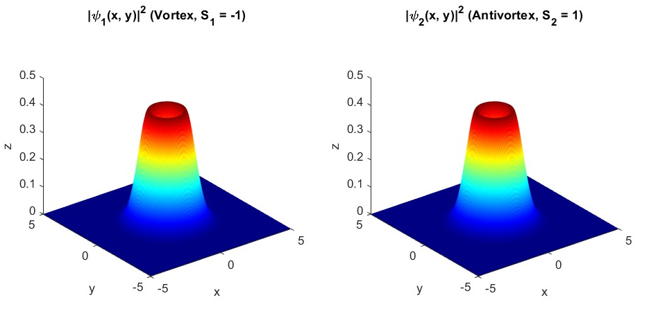
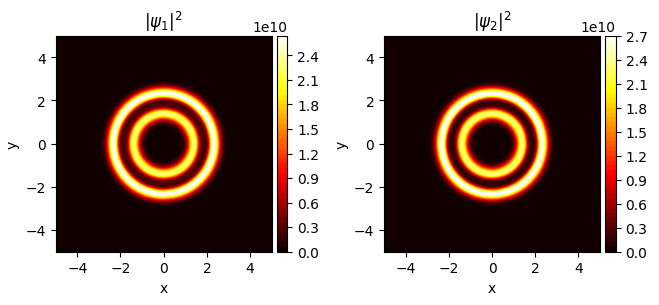
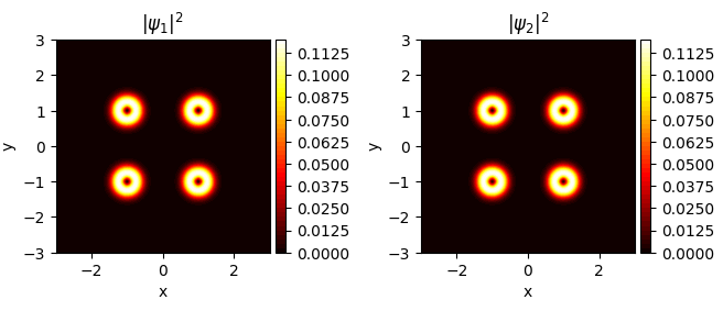
To demonstrate the formation of a single VAV bound state in the HO potential trap, we take interaction coefficients , . In this case, the VAV bound state exhibits the stable vortex pattern displayed in Fig. 3 by means of 2D contour density plot of for each component, in the plane. The lower panels of the figure represent the corresponding phase structures, viz., spirals winding around the vortex pivot. Further, the 3D profiles of the VAV bound state from Fig. 3 are plotted in Fig. 4. The VAV states, characterized by dependencies of their chemical potential on the SOC strength , which are plotted in Fig. 1, showing the comparison between the analytical and numerical findings. The analytical expression (15), with the nonlinearity-induced correction (16), is consistent with the numerical results, obtained by solving Eq. (13) for a fixed norm . Here we consider small , with the self-repulsion and cross-attraction nearly canceling each other through the Feshbach resonance. Recent work [91] have demonstrated similar tuning techniques in exciton-polariton systems. Figure 2 displays the chemical potential as a function of SOC strength , for distinct values of in-plane trapping frequency , using the analytical expression Eq. (15) with the nonlinearity-induced correction Eq. (16) for a fixed norm N=1.
a)\SetVerticalPole\imagecoffinleft3pt+\CoffinWidth\labelcoffin/2\SetVerticalPole\imagecoffinright\Width-3pt-\CoffinWidth\labelcoffin/2\SetHorizontalPole\imagecoffinup\Height-3pt-\CoffinHeight\labelcoffin/2\SetHorizontalPole\imagecoffindown3pt+\CoffinHeight\labelcoffin/2\JoinCoffins\imagecoffin[left,up]\labelcoffin[vc,hc]\TypesetCoffin\imagecoffin \SetHorizontalCoffin\imagecoffin \SetHorizontalCoffin\labelcoffinb)\SetVerticalPole\imagecoffinleft3pt+\CoffinWidth\labelcoffin/2\SetVerticalPole\imagecoffinright\Width-3pt-\CoffinWidth\labelcoffin/2\SetHorizontalPole\imagecoffinup\Height-3pt-\CoffinHeight\labelcoffin/2\SetHorizontalPole\imagecoffindown3pt+\CoffinHeight\labelcoffin/2\JoinCoffins\imagecoffin[left,up]\labelcoffin[vc,hc]\TypesetCoffin\imagecoffin \SetHorizontalCoffin\imagecoffin
 \SetHorizontalCoffin\labelcoffinc)\SetVerticalPole\imagecoffinleft3pt+\CoffinWidth\labelcoffin/2\SetVerticalPole\imagecoffinright\Width-3pt-\CoffinWidth\labelcoffin/2\SetHorizontalPole\imagecoffinup\Height-3pt-\CoffinHeight\labelcoffin/2\SetHorizontalPole\imagecoffindown3pt+\CoffinHeight\labelcoffin/2\JoinCoffins\imagecoffin[left,up]\labelcoffin[vc,hc]\TypesetCoffin\imagecoffin \SetHorizontalCoffin\imagecoffin
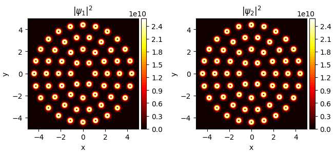 \SetHorizontalCoffin\labelcoffind)\SetVerticalPole\imagecoffinleft3pt+\CoffinWidth\labelcoffin/2\SetVerticalPole\imagecoffinright\Width-3pt-\CoffinWidth\labelcoffin/2\SetHorizontalPole\imagecoffinup\Height-3pt-\CoffinHeight\labelcoffin/2\SetHorizontalPole\imagecoffindown3pt+\CoffinHeight\labelcoffin/2\JoinCoffins\imagecoffin[left,up]\labelcoffin[vc,hc]\TypesetCoffin\imagecoffin \SetHorizontalCoffin\imagecoffin
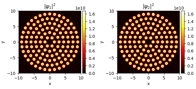 \SetHorizontalCoffin\labelcoffine)\SetVerticalPole\imagecoffinleft3pt+\CoffinWidth\labelcoffin/2\SetVerticalPole\imagecoffinright\Width-3pt-\CoffinWidth\labelcoffin/2\SetHorizontalPole\imagecoffinup\Height-3pt-\CoffinHeight\labelcoffin/2\SetHorizontalPole\imagecoffindown3pt+\CoffinHeight\labelcoffin/2\JoinCoffins\imagecoffin[left,up]\labelcoffin[vc,hc]\TypesetCoffin\imagecoffin
To create various lattice patterns built of multiple localized VAV elements (“pixels”), nonlinearity parameters and should be selected appropriately in Eq. (5), the initial state being selected as ring, circular, square, rectangle, hexagonal and triangular lattices. The study of these patterns begins with the ring and circular arrangements, represented in the polar coordinates. The trap is characterized by the in-plane and transverse trapping frequencies Hz and Hz, respectively, implying a less tight in-plane trap, that can accommodate a substantial number of particles and promote the formation of a circular pattern. As the interaction parameters and increase, the trap accumulates a greater number of particles, thus leading to the generation of an increasing number of individual VAV elements. To investigate the formation of a circular pattern, we take and , which produces a double-ring-shaped VAV mode, as shown in Fig. 5a) by means of contour plot of densities and in the plane. By augmenting the spacing between individual VAV pixels and maintaining with , the transition of the ring-shaped vortex to the circular array built of pixels is observed in Fig. 5b). Note that the creation of the latter configuration makes it necessary to use larger interaction parameters ( and ). For and , an annular pattern composed of pixels, with in the inner ring and in the outer one, is shown in Fig. 5c). Further increase to , with results in the pattern created of elements, including ones in the first ring, and , , and elements in the second, third, and fourth rings, as shown in Fig. 5d). For and , the pattern includes , , , and pixels in the first, second, third, and fourth rings, in addition to in the fifth one, as plotted in Fig. 5e) (for and , the annular pattern does not exhibit the fifth stable ring). In Figs. (5b) to (5e), we observe that the total number of VAV elements in each ring is , where is the ring’s number. Furthermore, in Figs. (5c) to (5e), radii of the succeeding rings grow by , while the position at the origin remains empty in all the patterns displayed in Fig. 5.
a)\SetVerticalPole\imagecoffinleft3pt+\CoffinWidth\labelcoffin/2\SetVerticalPole\imagecoffinright\Width-3pt-\CoffinWidth\labelcoffin/2\SetHorizontalPole\imagecoffinup\Height-3pt-\CoffinHeight\labelcoffin/2\SetHorizontalPole\imagecoffindown3pt+\CoffinHeight\labelcoffin/2\JoinCoffins\imagecoffin[left,up]\labelcoffin[vc,hc]\TypesetCoffin\imagecoffin \SetHorizontalCoffin\imagecoffin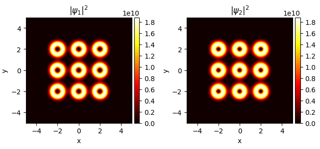 \SetHorizontalCoffin\labelcoffinb)\SetVerticalPole\imagecoffinleft3pt+\CoffinWidth\labelcoffin/2\SetVerticalPole\imagecoffinright\Width-3pt-\CoffinWidth\labelcoffin/2\SetHorizontalPole\imagecoffinup\Height-3pt-\CoffinHeight\labelcoffin/2\SetHorizontalPole\imagecoffindown3pt+\CoffinHeight\labelcoffin/2\JoinCoffins\imagecoffin[left,up]\labelcoffin[vc,hc]\TypesetCoffin\imagecoffin \SetHorizontalCoffin\imagecoffin
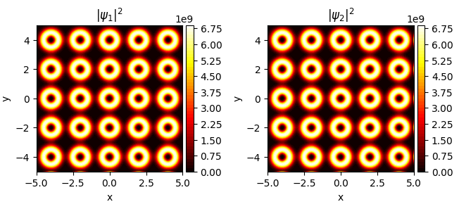 \SetHorizontalCoffin\labelcoffinc)\SetVerticalPole\imagecoffinleft3pt+\CoffinWidth\labelcoffin/2\SetVerticalPole\imagecoffinright\Width-3pt-\CoffinWidth\labelcoffin/2\SetHorizontalPole\imagecoffinup\Height-3pt-\CoffinHeight\labelcoffin/2\SetHorizontalPole\imagecoffindown3pt+\CoffinHeight\labelcoffin/2\JoinCoffins\imagecoffin[left,up]\labelcoffin[vc,hc]\TypesetCoffin\imagecoffin \SetHorizontalCoffin\imagecoffin
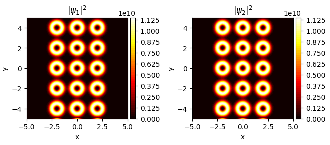 \SetHorizontalCoffin\labelcoffind)\SetVerticalPole\imagecoffinleft3pt+\CoffinWidth\labelcoffin/2\SetVerticalPole\imagecoffinright\Width-3pt-\CoffinWidth\labelcoffin/2\SetHorizontalPole\imagecoffinup\Height-3pt-\CoffinHeight\labelcoffin/2\SetHorizontalPole\imagecoffindown3pt+\CoffinHeight\labelcoffin/2\JoinCoffins\imagecoffin[left,up]\labelcoffin[vc,hc]\TypesetCoffin\imagecoffin \SetHorizontalCoffin\imagecoffin
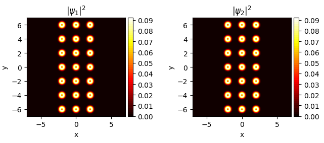 \SetHorizontalCoffin\labelcoffine)\SetVerticalPole\imagecoffinleft3pt+\CoffinWidth\labelcoffin/2\SetVerticalPole\imagecoffinright\Width-3pt-\CoffinWidth\labelcoffin/2\SetHorizontalPole\imagecoffinup\Height-3pt-\CoffinHeight\labelcoffin/2\SetHorizontalPole\imagecoffindown3pt+\CoffinHeight\labelcoffin/2\JoinCoffins\imagecoffin[left,up]\labelcoffin[vc,hc]\TypesetCoffin\imagecoffin
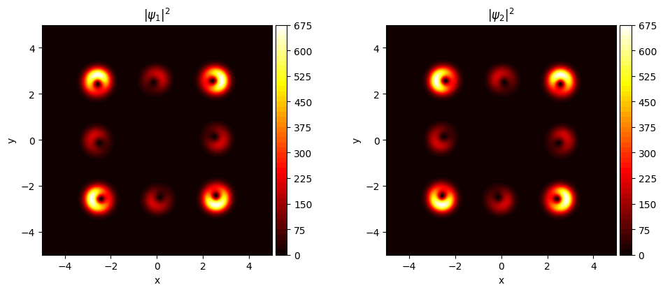
Next, we address square- and rectangular-lattice configurations of size maintained by the HO trap. Some of these configurations, were obtained for low values of interaction coefficients. In comparison to the circular lattices displayed in Fig. 5, much smaller values of and are sufficient to create square-lattice patterns. Figure (6a) displays contour plots of 2D density profiles in the plane for and , with the same SOC strength as fixed above, . Under these conditions, in Fig. 6a) the system produces a square-lattice structure with the empty position at the origin. For and and , a square lattice, built of VAV pixels (with one occupying the central position) is observed in Fig. 6b). Next, the lattice state is displayed in Fig. 6c), for and . It is composed of pixels, including one located at the center.
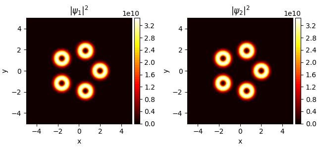
Stable rectangular lattices composed of and VAV elements are displayed in Figs. (6d) and (6e). The respective values of the nonlinearity parameters are , and , , respectively. Finally, we demonstrate stable pentagonal, hexagonal, and triangular lattices composed of VAV pixels. Actually, the hexagonal pattern may be considered as a triangular lattice with vacant central positions. Therefore, with inappropriate initial condition or parameter values, the numerical calculations may instead converge to circular or triangular states, by filling the vacant positions. For and , the pentagonal ring-shaped chain, consisting of five VAV elements, is depicted in Fig. 7a). The double pentagonal chain, plotted in Fig. 7b), corresponds to and . For and , the body-centered structure displayed in Fig. 7c) exhibits six elements forming a hexagonal cell, and one placed at the central location. In Fig. 7d), the hexagonal structure is transformed into a triangle configuration (which also seems as a rhombus) by adding two VAV elements at lateral positions (along the axis), in the case of and , so that the total number of the elements (pixels) in the configuration is nine. In Fig. 7e), the triangular lattice is further expanded to comprise elements, at and . Finally, Fig. 7f) demonstrates that the system with very large nonlinearity coefficients, such as and , maintains very large perfect triangular lattices. In particular, the one shown in Fig. 7f) is composed of VAV pixels arranged in four rows of pixels and three rows of ones.
Now, the investigation is carried out for the VAV pixels under strong isotropic confinement, with , in square-shaped, rectangular, and circular configurations. We initially discuss a square lattice configuration under the strong confinement, with an in-plane trapping frequency Hz and a transverse trapping frequency Hz. The interaction coefficients are set as and , as illustrated in Fig. 8a). We observe that the square-shaped lattice is not fully compatible with the isotropic trap, whereas the simpler configuration is. When subjected to the stronger isotropic confinement, the system eliminates the interstitial pixels, transforming the lattice into a configuration that better aligns with the isotropic trap. Figure 8b) illustrates a rectangular lattice configuration under in-plane and transverse trapping frequencies Hz and Hz. While the lattice is initiated as a structure with the central site, the limited available space prevents the central site from fully developing, and some sites also fail to exhibit a complete vortex profile. Finally, a circular vortex configuration represented in Fig. 8c) is investigated under the confinement with Hz and Hz, with interaction parameters and . As expected, the strong confinement makes the inner vortex ring less visible, due to insufficient space for its formation. As the confinement strengthens, the density in the trap significantly increases, restricting the ability of the vortices to rearrange freely. Additionally, the high density suppresses the formation of well-defined vortices, as the limited space restricts their full development.
a)\SetVerticalPole\imagecoffinleft3pt+\CoffinWidth\labelcoffin/2\SetVerticalPole\imagecoffinright\Width-3pt-\CoffinWidth\labelcoffin/2\SetHorizontalPole\imagecoffinup\Height-3pt-\CoffinHeight\labelcoffin/2\SetHorizontalPole\imagecoffindown3pt+\CoffinHeight\labelcoffin/2\JoinCoffins\imagecoffin[left,up]\labelcoffin[vc,hc]\TypesetCoffin\imagecoffin \SetHorizontalCoffin\imagecoffin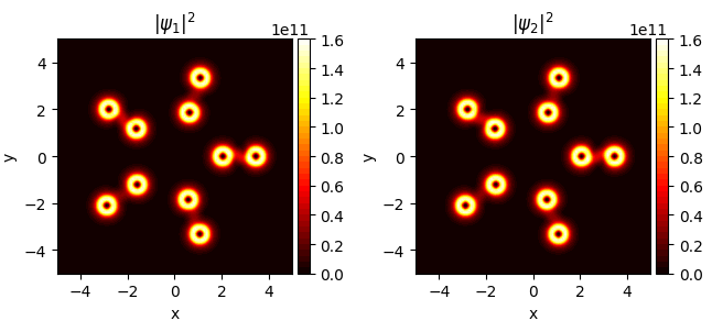 \SetHorizontalCoffin\labelcoffinb)\SetVerticalPole\imagecoffinleft3pt+\CoffinWidth\labelcoffin/2\SetVerticalPole\imagecoffinright\Width-3pt-\CoffinWidth\labelcoffin/2\SetHorizontalPole\imagecoffinup\Height-3pt-\CoffinHeight\labelcoffin/2\SetHorizontalPole\imagecoffindown3pt+\CoffinHeight\labelcoffin/2\JoinCoffins\imagecoffin[left,up]\labelcoffin[vc,hc]\TypesetCoffin\imagecoffin \SetHorizontalCoffin\imagecoffin
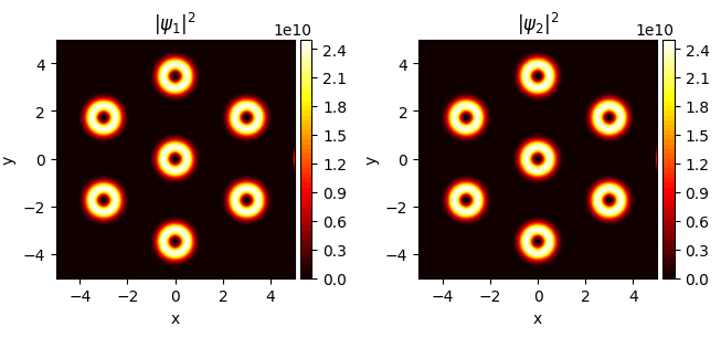 \SetHorizontalCoffin\labelcoffinc)\SetVerticalPole\imagecoffinleft3pt+\CoffinWidth\labelcoffin/2\SetVerticalPole\imagecoffinright\Width-3pt-\CoffinWidth\labelcoffin/2\SetHorizontalPole\imagecoffinup\Height-3pt-\CoffinHeight\labelcoffin/2\SetHorizontalPole\imagecoffindown3pt+\CoffinHeight\labelcoffin/2\JoinCoffins\imagecoffin[left,up]\labelcoffin[vc,hc]\TypesetCoffin\imagecoffin \SetHorizontalCoffin\imagecoffin
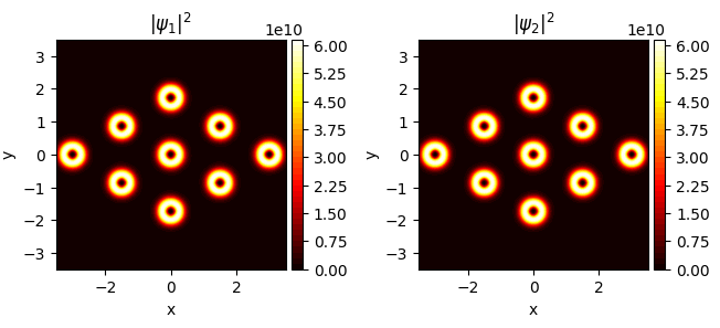 \SetHorizontalCoffin\labelcoffind)\SetVerticalPole\imagecoffinleft3pt+\CoffinWidth\labelcoffin/2\SetVerticalPole\imagecoffinright\Width-3pt-\CoffinWidth\labelcoffin/2\SetHorizontalPole\imagecoffinup\Height-3pt-\CoffinHeight\labelcoffin/2\SetHorizontalPole\imagecoffindown3pt+\CoffinHeight\labelcoffin/2\JoinCoffins\imagecoffin[left,up]\labelcoffin[vc,hc]\TypesetCoffin\imagecoffin \SetHorizontalCoffin\imagecoffin
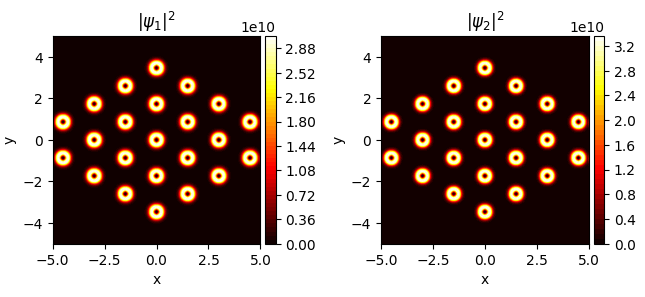 \SetHorizontalCoffin\labelcoffine)\SetVerticalPole\imagecoffinleft3pt+\CoffinWidth\labelcoffin/2\SetVerticalPole\imagecoffinright\Width-3pt-\CoffinWidth\labelcoffin/2\SetHorizontalPole\imagecoffinup\Height-3pt-\CoffinHeight\labelcoffin/2\SetHorizontalPole\imagecoffindown3pt+\CoffinHeight\labelcoffin/2\JoinCoffins\imagecoffin[left,up]\labelcoffin[vc,hc]\TypesetCoffin\imagecoffin \SetHorizontalCoffin\imagecoffin
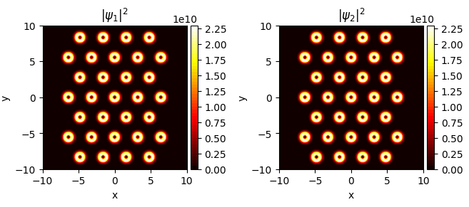 \SetHorizontalCoffin\labelcoffinf)\SetVerticalPole\imagecoffinleft3pt+\CoffinWidth\labelcoffin/2\SetVerticalPole\imagecoffinright\Width-3pt-\CoffinWidth\labelcoffin/2\SetHorizontalPole\imagecoffinup\Height-3pt-\CoffinHeight\labelcoffin/2\SetHorizontalPole\imagecoffindown3pt+\CoffinHeight\labelcoffin/2\JoinCoffins\imagecoffin[left,up]\labelcoffin[vc,hc]\TypesetCoffin\imagecoffin
a)\SetVerticalPole\imagecoffinleft3pt+\CoffinWidth\labelcoffin/2\SetVerticalPole\imagecoffinright\Width-3pt-\CoffinWidth\labelcoffin/2\SetHorizontalPole\imagecoffinup\Height-3pt-\CoffinHeight\labelcoffin/2\SetHorizontalPole\imagecoffindown3pt+\CoffinHeight\labelcoffin/2\JoinCoffins\imagecoffin[left,up]\labelcoffin[vc,hc]\TypesetCoffin\imagecoffin \SetHorizontalCoffin\imagecoffin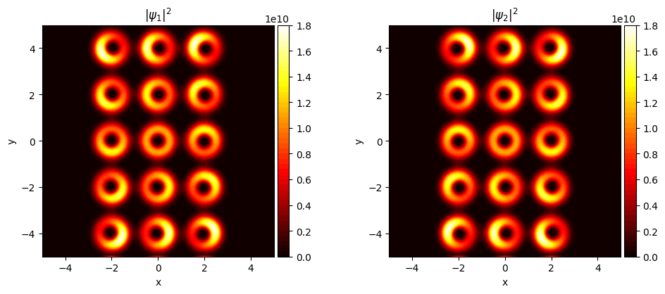 \SetHorizontalCoffin\labelcoffinb)\SetVerticalPole\imagecoffinleft3pt+\CoffinWidth\labelcoffin/2\SetVerticalPole\imagecoffinright\Width-3pt-\CoffinWidth\labelcoffin/2\SetHorizontalPole\imagecoffinup\Height-3pt-\CoffinHeight\labelcoffin/2\SetHorizontalPole\imagecoffindown3pt+\CoffinHeight\labelcoffin/2\JoinCoffins\imagecoffin[left,up]\labelcoffin[vc,hc]\TypesetCoffin\imagecoffin \SetHorizontalCoffin\imagecoffin
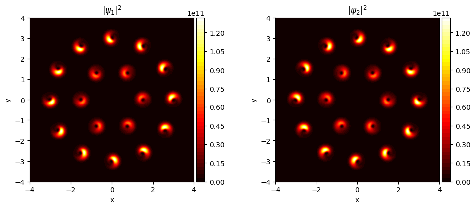 \SetHorizontalCoffin\labelcoffinc)\SetVerticalPole\imagecoffinleft3pt+\CoffinWidth\labelcoffin/2\SetVerticalPole\imagecoffinright\Width-3pt-\CoffinWidth\labelcoffin/2\SetHorizontalPole\imagecoffinup\Height-3pt-\CoffinHeight\labelcoffin/2\SetHorizontalPole\imagecoffindown3pt+\CoffinHeight\labelcoffin/2\JoinCoffins\imagecoffin[left,up]\labelcoffin[vc,hc]\TypesetCoffin\imagecoffin
IV Conclusion
In the framework of the 2D mean-field model of EP (exciton-polariton) condensates, we have performed the analysis of the formation of the single VAV (vortex-antivortex) two-component bound state, and lattices build of several or many VAV elements (“pixels”) under the action of the photonic SOC (spin-orbit coupling), represented by the second-order differential operator , and in-plane HO (harmonic-oscillator) trapping potential. The model is considered in the conservative form under the condition of the compensation of losses and pump. Making use of the trap’s capacity to accommodate a substantial number of particles, the examination of various lattice patterns was conducted, utilizing appropriate values of the interaction strengths and and other parameters. The study of various VAV lattices begins with circular patterns composed of two concentric rings. Further, circular lattices built of VAV elements were found as single- and multi-layer patterns, with the number of elements in each circular layer being a multiple of . Then, square and rectangular lattices, composed of the same VAV elements, were investigated. The lowest lattice state, with the unoccupied central position, was constructed for and , while the lattice, composed of VAV pixels, was constructed for and , exhibiting the occupied central position. Stable rectangular lattices of sizes and were found for , and , , respectively. The formation of pentagonal, hexagonal and triangular VAV lattices was addressed too. Triangular lattices were found at large values of the interaction parameters. A stable pentagonal ring was produced for and , while a double pentagonal ring employs and . The hexagonal lattice was produced for the respective minimum values of the coefficients, and , composed of six VAV pixels forming the hexagonal cell, with an extra pixel placed at the center. To construct the triangular lattice state composed of nine elements, by adding two elements to the hexagonal cell, and had to be set to large values, viz., and , respectively. To add an extra layer to the triangular lattice, making the total number of constituent VAV pixels equal to , the interaction coefficients were further ramped up to and . With very large values of the nonlinearity coefficients, and , a large stable triangular lattice, composed of elements, was found. The odd number of constituents takes place in those patterns which include a VAV pixel occupying the center’s position. The formation of the various lattice patterns in our system is determined by the interaction coefficients and initial conditions, with a critical density required for the creation of stable patterns being proportional to the interaction coefficients. Different configurations require disparate interaction levels: in the circular patterns, the lattice keeps the center empty, leading to a more uniform density distribution, whereas in hexagonal and triangular configurations the center is occupied, necessitating to use stronger interactions to reach the critical density for the pattern formation. It is remarkable that the various lattice patterns, which were previously reported in free-space models, persist under the action of the weak HO trap. They exhibit dynamical robustness and suggest additional theoretical and experimental studies. Further, we investigated the behavior of VAV pixels under the action of the strong isotropic confinement in different geometries, including square-shaped, rectangular, and circular arrangements. Our findings reveal that a square lattice is not fully compatible with the isotropic trapping for the in-plane and transverse trapping frequencies Hz and Hz, as stronger confinement leads to the elimination of interstitial pixels, resulting in a more stable configuration. Similarly, for a rectangular lattice with Hz and Hz, spatial constraints prevent the full development of certain vortex sites, particularly in the central region. Finally, for a circular vortex configuration, the strong confinement with Hz and Hz suppresses the inner vortex ring, restricting the free rearrangement of vortices due to increased density in the trap. The stability of these patterns should permit access to them in the experiment by choosing appropriate initial conditions in EP systems featuring the underlying TE-TM splitting.
The analysis may be enhanced by incorporating the Zeeman splitting between
the two components of the spinor wave function [92, 93]. It would be interesting to further explore the interaction between two VAV pixels with opposite polarities, i.e., one with vorticities and the other one with . Since these configurations are expected to interact attractively, they may form bound states such as mutually orbiting vortex pairs. Future work may focus on analyzing such interactions in greater detail to understand the formation of more complex vortex structures. Further extension may include the examination of lattice patterns composed of VAV pixels in dissipative
SOC systems, where a variety of spatially periodic states may be expected
[94, 95].
Acknowledgment: S. Sanjay and S. Saravana Veni acknowledge Amrita
Vishwa Vidyapeetham, Coimbatore, where this work was supported under Amrita
Seed Grant (File Number: ASG2022141). The work of B. A. Malomed was
supported, in part, by the Israel Science Foundation through grant No.
1695/22.
References
- Boninsegni and Prokof’ev [2012] M. Boninsegni, N. V. Prokof’ev, Colloquium: Supersolids: What and where are they?, Rev. Mod. Phys. 84 (2012) 759–776.
- Recati and Stringari [2023] A. Recati, S. Stringari, Supersolidity in ultracold dipolar gases, Nat. Rev. Phys. 5 (2023) 735–743.
- Ilzhöfer et al. [2021] P. Ilzhöfer, M. Sohmen, G. Durastante, C. Politi, A. Trautmann, G. Natale, G. Morpurgo, T. Giamarchi, L. Chomaz, M. Mark, et al., Phase coherence in out-of-equilibrium supersolid states of ultracold dipolar atoms, Nat. Phys. 17 (2021) 356–361.
- Verhelst and Tempere [2017] N. Verhelst, J. Tempere, Vortex structures in ultra-cold atomic gases, Vortex Dynamics and Optical Vortices, edited by H. Perez-de-Tejada, (INTECH) (2017) 1.
- Klaus et al. [2022] L. Klaus, T. Bland, E. Poli, C. Politi, G. Lamporesi, E. Casotti, R. N. Bisset, M. J. Mark, F. Ferlaino, Observation of vortices and vortex stripes in a dipolar condensate, Nat. Phys. 18 (2022) 1453–1458.
- Chaika et al. [2023] A. Chaika, A. Richaud, A. Yakimenko, Making ghost vortices visible in two-component bose-einstein condensates, Phys. Rev. Res. 5 (2023) 023109.
- Bulgac [2002] A. Bulgac, Dilute quantum droplets, Phys. Rev. Lett. 89 (2002) 050402.
- Luo et al. [2021] Z.-H. Luo, W. Pang, B. Liu, Y.-Y. Li, B. A. Malomed, A new form of liquid matter: Quantum droplets, Front. Phys. 16 (2021) 1–21.
- Guo and Pfau [2021] M. Guo, T. Pfau, A new state of matter of quantum droplets, Front. Phys. 16 (2021) 32202.
- Neely et al. [2010] T. W. Neely, E. C. Samson, A. S. Bradley, M. J. Davis, B. P. Anderson, Observation of vortex dipoles in an oblate bose-einstein condensate, Phys. Rev. Lett. 104 (2010) 160401.
- Weiler et al. [2008] C. N. Weiler, T. W. Neely, D. R. Scherer, A. S. Bradley, M. J. Davis, B. P. Anderson, Spontaneous vortices in the formation of bose–einstein condensates, Nature 455 (2008) 948–951.
- Petrov [2015] D. Petrov, Quantum mechanical stabilization of a collapsing bose-bose mixture, Phys. Rev. Lett. 115 (2015) 155302.
- Petrov and Astrakharchik [2016] D. Petrov, G. Astrakharchik, Ultradilute low-dimensional liquids, Phys. Rev. Lett. 117 (2016) 100401.
- Cheiney et al. [2018] P. Cheiney, C. Cabrera, J. Sanz, B. Naylor, L. Tanzi, L. Tarruell, Bright soliton to quantum droplet transition in a mixture of bose-einstein condensates, Phys. Rev. Lett. 120 (2018) 135301.
- Semeghini et al. [2018] G. Semeghini, G. Ferioli, L. Masi, C. Mazzinghi, L. Wolswijk, F. Minardi, M. Modugno, G. Modugno, M. Inguscio, M. Fattori, Self-bound quantum droplets of atomic mixtures in free space, Phys. Rev. Lett. 120 (2018) 235301.
- D’Errico et al. [2019] C. D’Errico, A. Burchianti, M. Prevedelli, L. Salasnich, F. Ancilotto, M. Modugno, F. Minardi, C. Fort, Observation of quantum droplets in a heteronuclear bosonic mixture, Phys. Rev. Res. 1 (2019) 033155.
- Burchianti et al. [2020] A. Burchianti, C. D’Errico, M. Prevedelli, L. Salasnich, F. Ancilotto, M. Modugno, F. Minardi, C. Fort, A dual-species bose-einstein condensate with attractive interspecies interactions, Condens. Matter 5 (2020) 21.
- Katsimiga et al. [2023] G. C. Katsimiga, S. I. Mistakidis, B. A. Malomed, D. J. Frantzeskakis, R. Carretero-Gonzalez, P. G. Kevrekidis, Interactions and dynamics of one-dimensional droplets, bubbles and kinks, Condens. Matter 8 (2023) 67.
- Hu et al. [2022] Y. Hu, Y. Fei, X.-L. Chen, Y. Zhang, Collisional dynamics of symmetric two-dimensional quantum droplets, Front. Phys. 17 (2022) 61505.
- Ferioli et al. [2019] G. Ferioli, G. Semeghini, L. Masi, G. Giusti, G. Modugno, M. Inguscio, A. Gallemí, A. Recati, M. Fattori, Collisions of self-bound quantum droplets, Phys. Rev. Lett. 122 (2019) 090401.
- Debnath et al. [2023] A. Debnath, A. Khan, B. Malomed, Interaction of one-dimensional quantum droplets with potential wells and barriers, Commun. Nonlinear Sci. Numer. Simul. 126 (2023) 107457.
- Schmitt et al. [2016] M. Schmitt, M. Wenzel, F. Böttcher, I. Ferrier-Barbut, T. Pfau, Self-bound droplets of a dilute magnetic quantum liquid, Nature 539 (2016) 259–262.
- Ferrier-Barbut et al. [2016] I. Ferrier-Barbut, H. Kadau, M. Schmitt, M. Wenzel, T. Pfau, Observation of quantum droplets in a strongly dipolar bose gas, Phys. Rev. Lett. 116 (2016) 215301.
- Wächtler and Santos [2016] F. Wächtler, L. Santos, Ground-state properties and elementary excitations of quantum droplets in dipolar bose-einstein condensates, Phys. Rev. A 94 (2016) 043618.
- Xi and Saito [2016] K.-T. Xi, H. Saito, Droplet formation in a bose-einstein condensate with strong dipole-dipole interaction, Phys. Rev. A 93 (2016) 011604.
- Böttcher et al. [2019] F. Böttcher, M. Wenzel, J.-N. Schmidt, M. Guo, T. Langen, I. Ferrier-Barbut, T. Pfau, R. Bombín, J. Sánchez-Baena, J. Boronat, et al., Dilute dipolar quantum droplets beyond the extended gross-pitaevskii equation, Phys. Rev. Res. 1 (2019) 033088.
- Young-S and Adhikari [2022a] L. E. Young-S, S. Adhikari, Supersolid-like square-and honeycomb-lattice crystallization of droplets in a dipolar condensate, Phys. Rev. A 105 (2022a) 033311.
- Young-S and Adhikari [2022b] L. E. Young-S, S. Adhikari, Supersolid-like square-and triangular-lattice crystallization of dipolar droplets in a box trap, Eur. Phys. J. Plus 137 (2022b) 1153.
- Young-S and Adhikari [2023] L. E. Young-S, S. Adhikari, Mini droplet, mega droplet and stripe formation in a dipolar condensate, Physica D 455 (2023) 133910.
- Li et al. [2018] Y. Li, Z. Chen, Z. Luo, C. Huang, H. Tan, W. Pang, B. A. Malomed, Two-dimensional vortex quantum droplets, Phys. Rev. A 98 (2018) 063602.
- Dong et al. [2022a] L. Dong, K. Shi, C. Huang, Internal modes of two-dimensional quantum droplets, Phys. Rev. A 106 (2022a) 053303.
- Dong et al. [2022b] L. Dong, D. Liu, Z. Du, K. Shi, W. Qi, Bistable multipole quantum droplets in binary bose-einstein condensates, Phys. Rev. A 105 (2022b) 033321.
- Kartashov et al. [2018] Y. V. Kartashov, B. A. Malomed, L. Tarruell, L. Torner, Three-dimensional droplets of swirling superfluids, Phys. Rev. A 98 (2018) 013612.
- Li et al. [2024] G. Li, Z. bin Zhao, B. Liu, Y. Li, Y. V. Kartashov, B. A. Malomed, Can vortex quantum droplets be realized experimentally?, Front. Phys. (2024). URL: https://api.semanticscholar.org/CorpusID:272686726.
- Cidrim et al. [2018] A. Cidrim, F. E. dos Santos, E. A. Henn, T. Macrì, Vortices in self-bound dipolar droplets, Phys. Rev. A 98 (2018) 023618.
- Dong et al. [2024] L. Dong, M. Fan, B. A. Malomed, Three-dimensional vortex and multipole quantum droplets in a toroidal potential, Chaos, Solitons & Fractals 188 (2024) 115499.
- Dong et al. [2023] L. Dong, M. Fan, B. A. Malomed, Stable higher-charge vortex solitons in the cubic–quintic medium with a ring potential, Opt. Lett. 48 (2023) 4817–4820.
- Dong et al. [2024] L. Dong, M. Fan, B. A. Malomed, Stable higher-order vortex quantum droplets in an annular potential, Chaos, Solitons & Fractals 179 (2024) 114472.
- Dong et al. [2023] L. Dong, M. Fan, C. Huang, B. A. Malomed, Multipole solitons in competing nonlinear media with an annular potential, Phys. Rev. A 108 (2023) 063501.
- Tabi CB, Tagwo H, Latchio Tiofack CG, Veni S and Kofané TC [2025] Tabi CB, Tagwo H, Latchio Tiofack CG, Veni S and Kofané TC, Coupled wave instability in pure-quartic dispersive and noninstantaneous Kerr media in presence of walk-off, Phys. Lett. A 529 (2025) 130066.
- Veni SS, Rajan MSM, Tabi CB and Kofané TC [2024] Veni SS, Rajan MSM, Tabi CB and Kofané TC, Numerical investigation on nonautonomous optical rogue waves and Modulation Instability analysis for a nonautonomous system, Phys. Scr. 99 (2024) 025202.
- Tabi CB, Veni S, Wamba E, and Kofané TC [2023] Tabi CB, Veni S, Wamba E, and Kofané TC, Modulational instability and droplet formation in Bose-Bose mixtures with Lee-Huang-Yang correction and polaron-like impurity, Phys. Lett. A 485 (2023) 129087.
- Li et al. [2017] Y. Li, Z. Luo, Y. Liu, Z. Chen, C. Huang, S. Fu, H. Tan, B. A. Malomed, Two-dimensional solitons and quantum droplets supported by competing self-and cross-interactions in spin-orbit-coupled condensates, New J. Phys. 19 (2017) 113043.
- Cui [2018] X. Cui, Spin-orbit-coupling-induced quantum droplet in ultracold bose-fermi mixtures, Phys. Rev. A 98 (2018) 023630.
- Gangwar et al. [2024] S. Gangwar, R. Ravisankar, S. Mistakidis, P. Muruganandam, P. K. Mishra, Spectrum and quench-induced dynamics of spin-orbit-coupled quantum droplets, Phys. Rev. A 109 (2024) 013321.
- Xu et al. [2024] S.-D. Xu, J. Wang, M.-Z. Zhou, L.-L. Mi, A.-X. Zhang, J.-K. Xue, The polarized and unpolarized spin-orbit coupled quantum droplets in a harmonic trap, Phys. Lett. A 522 (2024) 129777.
- Sakaguchi and Li [2013] H. Sakaguchi, B. Li, Vortex lattice solutions to the gross-pitaevskii equation with spin-orbit coupling in optical lattices, Phys. Rev. A 87 (2013) 015602.
- Sakaguchi et al. [2014] H. Sakaguchi, B. Li, B. A. Malomed, Creation of two-dimensional composite solitons in spin-orbit-coupled self-attractive bose-einstein condensates in free space, Phys. Rev. E 89 (2014) 032920.
- Meng et al. [2016] Z. Meng, L. Huang, P. Peng, D. Li, L. Chen, Y. Xu, C. Zhang, P. Wang, J. Zhang, Experimental observation of a topological band gap opening in ultracold fermi gases with two-dimensional spin-orbit coupling, Phys. Rev. Lett. 117 (2016) 235304.
- Zhang et al. [2016] Y. Zhang, M. E. Mossman, T. Busch, P. Engels, C. Zhang, Properties of spin–orbit-coupled bose–einstein condensates, Front. Phys. 11 (2016) 1–28.
- Zhong et al. [2018] R.-X. Zhong, Z.-P. Chen, C.-Q. Huang, Z.-H. Luo, H.-S. Tan, B. A. Malomed, Y.-Y. Li, Self-trapping under two-dimensional spin-orbit coupling and spatially growing repulsive nonlinearity, Front. Phys. 13 (2018) 1–16.
- Wang et al. [2024] Y. Wang, J. Cui, H. Zhang, Y. Zhao, S. Xu, Q. Zhou, Rydberg-induced topological solitons in three-dimensional rotation spin–orbit-coupled bose–einstein condensates, Chin. Phys. Lett. 41 (2024) 090302.
- Zhao et al. [2024] Y. Zhao, Q. Huang, T. Gong, S. Xu, Z. Li, B. A. Malomed, Three-dimensional solitons supported by the spin–orbit coupling and rydberg–rydberg interactions in pt-symmetric potentials, Chaos, Solitons & Fractals 187 (2024) 115329.
- Kartashov et al. [2015] Y. V. Kartashov, B. A. Malomed, V. V. Konotop, V. E. Lobanov, L. Torner, Stabilization of spatiotemporal solitons in kerr media by dispersive coupling, Opt. Lett. 40 (2015) 1045–1048.
- Sakaguchi et al. [2017] H. Sakaguchi, B. A. Malomed, D. V. Skryabin, Spin–orbit coupling and nonlinear modes of the polariton condensate in a harmonic trap, New J. Phys. 19 (2017) 085003.
- Whittaker et al. [2018] C. Whittaker, E. Cancellieri, P. Walker, D. Gulevich, H. Schomerus, D. Vaitiekus, B. Royall, D. Whittaker, E. Clarke, I. Iorsh, et al., Exciton polaritons in a two-dimensional lieb lattice with spin-orbit coupling, Phys. Rev. Lett. 120 (2018) 097401.
- Klaas et al. [2019] M. Klaas, O. A. Egorov, T. Liew, A. Nalitov, V. Marković, H. Suchomel, T. Harder, S. Betzold, E. Ostrovskaya, A. Kavokin, et al., Nonresonant spin selection methods and polarization control in exciton-polariton condensates, Phys. Rev. B 99 (2019) 115303.
- Aristov et al. [2022] D. Aristov, H. Sigurdsson, P. G. Lagoudakis, Screening nearest-neighbor interactions in networks of exciton-polariton condensates through spin-orbit coupling, Phys. Rev. B 105 (2022) 155306.
- Li et al. [2022] Y. Li, X. Ma, X. Zhai, M. Gao, H. Dai, S. Schumacher, T. Gao, Manipulating polariton condensates by rashba-dresselhaus coupling at room temperature, Nat. Commun. 13 (2022) 3785.
- Dufferwiel et al. [2015] S. Dufferwiel, F. Li, E. Cancellieri, L. Giriunas, A. Trichet, D. Whittaker, P. Walker, F. Fras, E. Clarke, J. Smith, et al., Spin textures of exciton-polaritons in a tunable microcavity with large te-tm splitting, Phys. Rev. Lett. 115 (2015) 246401.
- Solnyshkov et al. [2021] D. D. Solnyshkov, G. Malpuech, P. St-Jean, S. Ravets, J. Bloch, A. Amo, Microcavity polaritons for topological photonics, Opt. Mater. Express 11 (2021) 1119–1142.
- Lovett et al. [2023] S. Lovett, P. M. Walker, A. Osipov, A. Yulin, P. U. Naik, C. E. Whittaker, I. A. Shelykh, M. S. Skolnick, D. N. Krizhanovskii, Observation of zitterbewegung in photonic microcavities, Light sci. appl. 12 (2023) 126.
- Ma et al. [2020] X. Ma, Y. V. Kartashov, A. Kavokin, S. Schumacher, Chiral condensates in a polariton hexagonal ring, Opt. Lett. 45 (2020) 5700.
- Cheng et al. [2024] S.-C. Cheng, S.-D. Jheng, T.-W. Chen, Topological excitation of exciton-polariton half-vortices and skyrmions in a magnetic field with te-tm splitting, Phys. Lett. A 512 (2024) 129600.
- Pukrop et al. [2020] M. Pukrop, S. Schumacher, X. Ma, Circular polarization reversal of half-vortex cores in polariton condensates, Phys. Rev. B 101 (2020) 205301.
- Cilibrizzi et al. [2016] P. Cilibrizzi, H. Sigurdsson, T. C. H. Liew, H. Ohadi, A. Askitopoulos, S. Brodbeck, C. Schneider, I. A. Shelykh, S. Höfling, J. Ruostekoski, et al., Half-skyrmion spin textures in polariton microcavities, Phys. Rev. B 94 (2016) 045315.
- Lagoudakis and Berloff [2017] P. G. Lagoudakis, N. G. Berloff, A polariton graph simulator, New J. Phys. 19 (2017) 125008.
- Liew and Rubo [2018] T. Liew, Y. Rubo, Quantum exciton-polariton networks through inverse four-wave mixing, Phys. Rev. B 97 (2018) 041302.
- Gnusov et al. [2023] I. Gnusov, S. Harrison, S. Alyatkin, K. Sitnik, J. Töpfer, H. Sigurdsson, P. Lagoudakis, Quantum vortex formation in the “rotating bucket” experiment with polariton condensates, Sci. Adv. 9 (2023) eadd1299.
- Yulin et al. [2020] A. Yulin, A. Nalitov, I. Shelykh, Spinning polariton vortices with magnetic field, Phys. Rev. B 101 (2020) 104308.
- Tosi et al. [2012] G. Tosi, G. Christmann, N. Berloff, P. Tsotsis, T. Gao, Z. Hatzopoulos, P. Savvidis, J. Baumberg, Sculpting oscillators with light within a nonlinear quantum fluid, Nat. Phys. 8 (2012) 190–194.
- Toledo Solano and Rubo [2010] M. Toledo Solano, Y. G. Rubo, Comment on “topological stability of the half-vortices in spinor exciton-polariton condensates”, Phys. Rev. B Condens. Matter 82 (2010) 127301.
- Flayac et al. [2010] H. Flayac, D. Solnyshkov, G. Malpuech, I. Shelykh, Reply to “comment on ‘topological stability of the half-vortices in spinor exciton-polariton condensates’”, Phys. Rev. B Condens. Matter 82 (2010) 127302.
- Lobanov et al. [2010] V. E. Lobanov, Y. V. Kartashov, V. A. Vysloukh, L. Torner, Stable radially symmetric and azimuthally modulated vortex solitons supported by localized gain, Opt. Lett. 36 (2010) 85–87.
- Toledo-Solano et al. [2014] M. Toledo-Solano, M. Mora-Ramos, A. Figueroa, Y. Rubo, Warping and interactions of vortices in exciton-polariton condensates, Phys. Rev. B 89 (2014) 035308.
- Madimabe et al. [2023] E. B. Madimabe, C. B. Tabi, C. G. L. Tiofack, T. C. Kofané, Modulational instability in vector exciton-polariton condensates with photonic spin-orbit coupling, Phys. Rev. B 107 (2023) 184502.
- Bobrovska and Matuszewski [2015] N. Bobrovska, M. Matuszewski, Adiabatic approximation and fluctuations in exciton-polariton condensates, Phys. Rev. B 92 (2015) 035311.
- Bobrovska et al. [2014] N. Bobrovska, E. A. Ostrovskaya, M. Matuszewski, Stability and spatial coherence of nonresonantly pumped exciton-polariton condensates, Phys. Rev. B 90 (2014) 205304.
- Tabi et al. [2024] C. B. Tabi, C. G. Latchio Tiofack, H. Tagwo, T. C. Kofané, Effect of weak nonlocal nonlinearity on generalized sixth-order dispersion modulational instability in optical media, Nonlinear Dyn. 112 (2024) 10341–10354.
- Karnieli et al. [2024] A. Karnieli, S. Tsesses, R. Yu, N. Rivera, A. Arie, I. Kaminer, S. Fan, Universal and ultrafast quantum computation based on free-electron-polariton blockade, PRX Quantum 5 (2024) 010339.
- Zhang et al. [2022] L. Zhang, J. Hu, J. Wu, R. Su, Z. Chen, Q. Xiong, H. Deng, Recent developments on polariton lasers, Prog. Quantum Electron. 83 (2022) 100399.
- Flayac et al. [2010] H. Flayac, I. Shelykh, D. Solnyshkov, G. Malpuech, Topological stability of the half-vortices in spinor exciton-polariton condensates, Phys. Rev. B 81 (2010) 045318.
- Dovzhenko et al. [2023] D. Dovzhenko, D. Aristov, L. Pickup, H. Sigurdsson, P. Lagoudakis, Next-nearest-neighbor coupling with spinor polariton condensates, Phys. Rev. B 108 (2023) L161301.
- Takemura et al. [2014] N. Takemura, S. Trebaol, M. Wouters, M. T. Portella-Oberli, B. Deveaud, Polaritonic feshbach resonance, Nat. Phys. 10 (2014) 500–504.
- Zezyulin et al. [2018] D. A. Zezyulin, Y. V. Kartashov, D. V. Skryabin, I. A. Shelykh, Spin–orbit coupled polariton condensates in a radially periodic potential: multiring vortices and rotating solitons, ACS Photonics 5 (2018) 3634–3642.
- Javanainen and Ruostekoski [2006] J. Javanainen, J. Ruostekoski, Symbolic calculation in development of algorithms: split-step methods for the gross–pitaevskii equation, J. Phys. A Math. Gen. 39 (2006) L179.
- Lakoba [2020] T. I. Lakoba, Study of instability of the fourier split-step method for the massive gross–neveu model, J. Comput. Phys. 402 (2020) 109100.
- Semenova et al. [2021] A. Semenova, S. A. Dyachenko, A. O. Korotkevich, P. M. Lushnikov, Comparison of split-step and hamiltonian integration methods for simulation of the nonlinear schrödinger type equations, J. Comput. Phys. 427 (2021) 110061.
- Young-S et al. [2023] L. E. Young-S, P. Muruganandam, A. Balaž, S. K. Adhikari, Openmp fortran programs for solving the time-dependent dipolar gross-pitaevskii equation, Comput. Phys. Commun. 286 (2023) 108669.
- Antoine et al. [2021] X. Antoine, J. Shen, Q. Tang, Scalar auxiliary variable/lagrange multiplier based pseudospectral schemes for the dynamics of nonlinear schrödinger/gross-pitaevskii equations, J. Comput. Phys. 437 (2021) 110328.
- Navadeh-Toupchi et al. [2019] M. Navadeh-Toupchi, N. Takemura, M. Anderson, D. Oberli, M. Portella-Oberli, Polaritonic cross feshbach resonance, Phys. Rev. Lett. 122 (2019) 047402.
- Nalitov et al. [2015] A. Nalitov, D. Solnyshkov, G. Malpuech, Polariton z topological insulator, Phys. Rev. Lett. 114 (2015) 116401.
- Karzig et al. [2015] T. Karzig, C. E. Bardyn, N. H. Lindner, G. Refael, Topological polaritons, Phys. Rev. X 5 (2015) 031001.
- Vercesi et al. [2023] F. Vercesi, Q. Fontaine, S. Ravets, J. Bloch, M. Richard, L. Canet, A. Minguzzi, Phase diagram of one-dimensional driven-dissipative exciton-polariton condensates, Phys. Rev. Res. 5 (2023) 043062.
- Chen and Cheng [2024] T.-W. Chen, S.-C. Cheng, Nonequilibrium spinor exciton-polariton condensates in a magnetic field, Phys. Scr. 99 (2024) 035534.