Through the Looking-Glass, and What AdS Found There:
quantum particle production with a Whittaker spectrum
Abstract
Parity-inverted anti-de Sitter space – “flipped AdS” – is studied through the accelerating boundary correspondence of a moving mirror trajectory. The particle production exhibits positive energy flux and a finite total energy (both unlike AdS). The particle spectrum is of Whittaker form, with some similarities to a Planck thermal spectrum. We also derive the corresponding spacetime metric, with similarities to regular de Sitter space, but exhibiting a tower of repeated causal regions with horizons.
I Introduction
The thermal particle spectrum and constant energy flux emitted by the moving mirror (accelerating boundary) corresponding to de Sitter spacetime [1] demonstrated that multiple different equations of motion can generate exact eternal Planck-distributed vacuum quanta, with the first such case identified by Carlitz and Willey [2] as an analog to black hole evaporation [3]. Leveraging the constant flux condition of the Möbius symmetry [4] inherent in the Davies-Fulling [5, 6] stress-tensor Schwarzian [7, 8], a third solution emerged – the anti-de Sitter (AdS) moving mirror – distinguished by its eternally negative energy flux [9, 10].
While the negative energy flux of the AdS trajectory is physically startling, it is nevertheless mathematically easy to obtain. Even the AdS equation of motion itself may be obtained simply from the dS trajectory by introducing an imaginary acceleration parameter [1], , reminiscent of a Wick rotation.
However, in 3+1 dimensions the particle production from an accelerating electron can only be fully captured by the moving mirror model [11, 12, 13, 14] when a parity flip is used to account for both sides of the mirror. Only then does an accurate analysis of photon production and emitted power ensue.
Thus, investigating the radiation on the opposite side of the moving mirror has yielded valuable insights consistent with experimental observations. In particular when horizons are present, which are impossible for a massive electron, a careful analysis is required to understand particle creation and the energy carried, e.g. [15]. Given the AdS mirror’s unique properties—negative energy flux, dual horizons, and asymptotic uniform acceleration—exploring its parity-flipped counterpart could provide further intriguing results. Moreover, since flipped AdS has no retarded time asymptote, we can test Walker’s [16] consistency between the total stress-energy from the flux – calculated from the mirror trajectory – and the sum of quanta given by the beta Bogoliubov coefficients.
In general, comparison between de Sitter, Anti-de Sitter, and flipped AdS behaviors could shed light on open questions regarding particle production, negative energy states, and asymptotic horizons or acceleration.
In Section II we explore the dynamics, including the velocity, acceleration, and spacetime structure of flipped AdS. Section III calculates the emitted flux and total energy. We compute the beta Bogoliubov coefficients in Section IV, producing the particle spectrum, and establish the consistency with the energy flux. Section V contrasts the flipped AdS particle spectrum with the usual AdS spectrum, and Section VI derives the spacetime metric equivalent to the flipped AdS mirror trajectory. We conclude in Section VII.
II Flipped AdS Dynamics
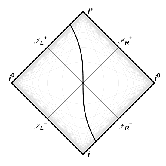
In light-cone coordinates, with retarded time and advanced time , the standard AdS mirror trajectory is . We define the flipped AdS mirror by a parity transformation, interchanging and , so that
| (1) |
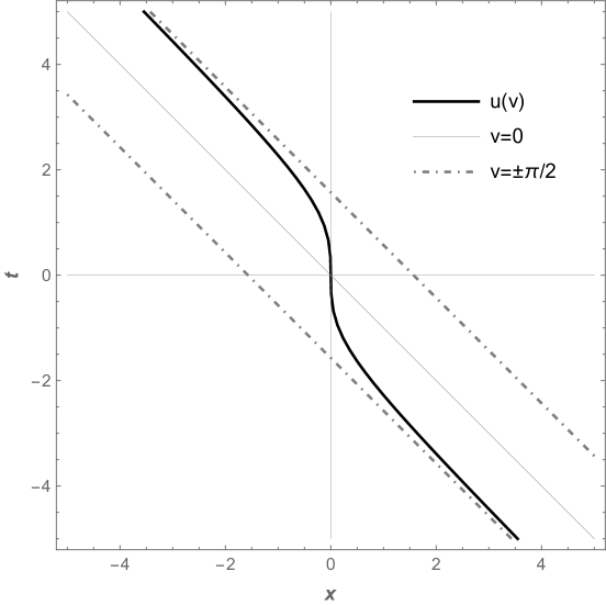
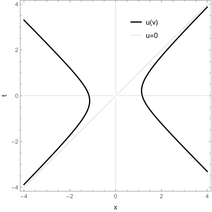
Figure 1 shows the worldline in a conformal diagram, and Figure 2 in a spacetime plot. Like the thermal mirror of de Sitter [1] and the thermal anti-de Sitter mirror [9] (eternal negative energy flux), the flipped AdS mirror has some physically interesting traits all on its own. One aspect is that it is unbounded in the retarded time (going to ), but bounded due to horizons in the advanced time , with .
The mirror velocity comes from the rapidity , giving
| (2) |
which in the limits or horizon limits of give
| (3) |
That is, the mirror (accelerating boundary) approaches the speed of light in the receding direction (to the left) away from the observer on the right-hand side near the horizon. At , the velocity vanishes.
The proper acceleration, , or , is
| (4) |
Now we can see the meaning of the quantity ; it is the asymptotically uniform (extremum) acceleration in the far past and far future:
| (5) |
III Radiated Energy
Accelerated boundaries, like black holes and spacetime horizons, give rise to quantum radiation of particles. The energy flux of radiated quanta from the accelerating boundary is [5, 7, 8]
| (6) |
or in terms of -coordinate is
| (7) |
These formulas reveal simple expressions for the energy flux from the flipped AdS mirror,
| (8) |
The total energy emission is
| (9) |
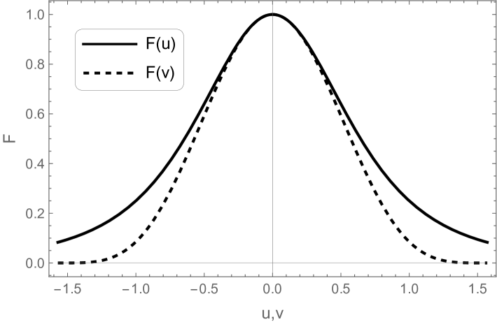
The mirror accelerates forever, yet the total energy emission is finite. Note that at the asymptotes the flux dies off as or . Figure 3 plots the energy flux.
Having established the total energy emission from the flux in Eq. (9), the next step is to derive the total energy from the particle creation at the quantum level, i.e., through the creation/annihilation operators or beta Bogoliubov coefficients. For this, we recall that Walker [16] demonstrated complete consistency between particle and energy production predictions. The total energy released can be found by adding each quantum,
| (10) |
where and are the outgoing and ingoing frequencies of the field modes subject to the accelerating boundary. The criteria for this to agree with the total stress-energy,
| (11) |
require the absence of a retarded time asymptote in the mirror’s trajectory (see the derivation of Eq. 5.4 in [16]).
The flipped AdS trajectory has no retarded time asymptote (cf. [1, 9]). Thus, Walker’s requirement is satisfied. In this case, it is also encouraging that the radiated stress-energy, Eq. (8),
| (12) |
is always positive and finite, rather than the negative flux of standard AdS. Adding quanta should intuitively work.
Naively, it might be unsurprising that the total stress-energy released could be computed by adding each quantum. It is nevertheless essential to confirm this. Why? Demonstrating consistency would contribute valuable intuition because for standard (nonflipped) AdS the energy flux and total energy,
| (13) |
are negative finite constants, which is interesting and physically unsettling.111For clarity, we use for the AdS mirror and for the flipped AdS mirror; they would be related by . Note that standard AdS does have a retarded time asymptote, and so fails the Walker criterion. (See Appendix A for more detail.) The unique form of flipped AdS’s positive and finite emission, Eq. (12), is the radiative counterpart to the AdS mirror’s time-independent emission of negative energy, Eq. (13).
IV Whittaker Spectrum
Now let us perform the energy summation over quantum modes and verify that it agrees with the stress-energy approach. We compute the beta Bogoliubov coefficient using the bounded integral in advanced time (see e.g. [7]),
| (14) |
after an integration by parts, and the boundary term vanishing due to the asymptotic structure. Plugging in our trajectory Eq. (1) gives
| (15) |
where the integration is zero. We may write , , , so that
| (16) |
Applying Gradshteyn & Ryzhik 3.718.6 [17],
| (17) |
which gives a Whittaker function, except that when is even then the integral and hence . Therefore, Eq. (16) is equal to
| (18) |
Note that is real, a consequence of being an odd function (see [18]), so
| (19) |
Adding up the energy of each quantum as in Eq. (10),
| (20) |
consistent with the energy emitted as derived by the stress-tensor, Eq. (9). Quantum summing works, as it should in this case.
V Whittaker vs. Planck
The emitted particle spectrum follows from the beta Bogoliubov coefficients by
| (21) |
and the energy spectrum is simply .
For the usual (“right hand side” of the) AdS mirror, the particle spectrum is Planckian, i.e. thermal (though the energy flux is negative). Consider that the integral of for a Planck distribution with gives the Planckian energy
| (22) |
which is the same as Eq. (9).
Despite the Planckian sum being the same as the Whittaker sum, the particle spectrum for the flipped AdS (or “left hand side”) mirror is not Planckian but rather of Whittaker form,
| Whittaker | (23) | ||||
| Planck | (24) |
Figure 4 compares these energy spectra.
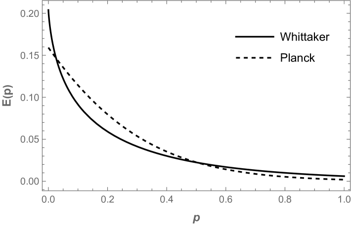
Table 1 summarizes several related accelerating mirror trajectories and their properties, including the total flux, total energy, and whether quantum summing applies.
| Mirrors | Flux | Energy | Quantum Sum Eq. (10) | |
|---|---|---|---|---|
| Carlitz-Willey | ||||
| Carlitz-Willey Flipped | invalid | |||
| de Sitter | ||||
| de Sitter Flipped | invalid | |||
| Anti-de Sitter | invalid | |||
| Anti-de Sitter Flipped | consistent! |
VI Spacetime Metric
Finally, we look at connecting the flipped AdS mirror to a spacetime, as can be done for the usual AdS and de Sitter cases. The accelerating boundary correspondence relates a mirror trajectory to a spacetime metric through matching conditions on null shells (see e.g. [1] for explicit demonstration for the de Sitter case). Carrying this out for our flipped AdS case, we obtain the cosmological, i.e. spacetime, metric
| (25) |
where and .
This bears definite similarities to the de Sitter metric in static coordinates, which has (see for example [19]). However, unlike the single cosmological horizon in de Sitter space at , flipped AdS has an infinite sequence of horizons located at
| (26) |
or with , the locations of the horizons are at , , , etc.
Far from the horizon, however, , the spacetimes appear the same, , with flipped AdS having an effective cosmological constant
| (27) |
At larger distances, the periodic nature of the flipped AdS introduces a novel layered structure with repeating causal regions, suggestive of cyclic222Recall that the beta Bogoliubov coefficients vanish for even, i.e. frequencies that are integer multiples of . or emergent cosmological models, e.g., [20, 21, 22].
VII Conclusions
Anti-de Sitter space plays a central and intriguing role in understanding fundamental physics and spacetime. The accelerating boundary correspondence to AdS yields thermal but negative energy flux. Here we parity invert, or “flip”, AdS and find interesting properties. The quantum energy emission is consistent, positive, and finite while the motion exhibits asymptotic uniform acceleration and no boundary asymptote in retarded time, though horizons in advanced time. Flipped AdS is the first explored particle production solution with these properties.
Flipped AdS particle production has beta Bogoliubov coefficients that can be solved analytically, delivering a particle spectrum involving a Whittaker function. Moreover the summed quanta energy can be explicitly shown to agree with the total energy flux, as it should due to lack of boundary in retarded time. While the Whittaker spectrum is nonthermal, the integrated energy agrees with that of a thermal Planck spectrum. Since the usual AdS solution has negative energy flux, the appearance of the Whittaker spectrum in the flipped AdS case could yield insights into negative energy creation and understanding quantum field behavior under extreme conditions.
Flipped AdS also has similarities to regular de Sitter space, with a cosmological, i.e. spacetime, metric that agrees with de Sitter far from the horizon. However flipped AdS actually has a tower of periodic spacetime horizons, suggestive of a cyclic universe. We can also preserve the flux properties of flipped AdS by a Möbius transform (specifically inversion) but change the spacetime structure to obtain asymptotes in retarded time (see Appendix B). These interconnections between AdS, flipped AdS, and de Sitter, and thermal, negative, and Whittaker particle creation, may be fruitful areas for further investigation.
Acknowledgements.
M.G. is supported, in part, by the FY2024-SGP-1-STMM Faculty Development Competitive Research Grant (FDCRGP) no.201223FD8824 and SSH20224004 at Nazarbayev University in Qazaqstan.Appendix A Retarded Time Asymptote and Standard vs Flipped AdS
To emphasize and clarify the role of the retarded time asymptote, or its lack, we consider an alternative approach to computing the emitted positive energy from flipped AdS. This method involves an integration by parts on the Davies-Fulling stress-energy, Eq. (6). The boundary term vanishes—as Walker predicts—because the mirror’s velocity asymptotically approaches , causing an advanced time asymptote, and the numerator tends to zero despite the proper acceleration remaining constant, leading to
| (28) |
Plugging in Eq. (1) then yields
| (29) |
This contrasts with the non-vanishing boundary term from the standard (nonflipped) AdS mirror due to a velocity approach to +1, which causes a divergence from the denominator, ultimately causing negative energy. The retarded time asymptote is the culprit and, overall, negative energy emission results. This negative sign spoils the ability to obtain the total emission by a sum of positive energies for each quantum from the standard AdS mirror. No such problem exists for the flipped AdS mirror, as we showed in Section IV.
Appendix B Hidden Horizons
A Möbius transform [4] of de Sitter’s mirror [1] gives the Carlitz-Willey [2] trajectory. Therefore let us explore the Möbius transform, , of the flipped AdS trajectory, specifically an inversion [4]. The inversion gives the following trajectory with as :
| (30) |
Figure 5 shows the trajectory in a spacetime diagram.
The flux emitted by an accelerating mirror following the trajectory is the same as that emitted in the case, Eq. (8), consistent with Möbius symmetry, so
| (31) |
despite the -asymptote. Nevertheless, due to the asymptote, the summation of quanta will not work.
References
- Good et al. [2020] M. R. R. Good, A. Zhakenuly, and E. V. Linder, Mirror at the edge of the universe: Reflections on an accelerated boundary correspondence with de Sitter cosmology, Phys. Rev. D 102, 045020 (2020), arXiv:2005.03850 [gr-qc] .
- Carlitz and Willey [1987] R. D. Carlitz and R. S. Willey, Reflections on moving mirrors, Phys. Rev. D 36, 2327 (1987).
- Hawking [1975] S. Hawking, Particle Creation by Black Holes, Commun. Math. Phys. 43, 199 (1975).
- Good and Linder [2022] M. R. R. Good and E. V. Linder, Möbius mirrors, Class. Quant. Grav. 39, 105003 (2022), arXiv:2108.07451 [gr-qc] .
- Fulling and Davies [1976] S. A. Fulling and P. C. W. Davies, Radiation from a moving mirror in two dimensional space-time: Conformal anomaly, Proc. R. Soc. Lond. A 348, 393 (1976).
- Davies and Fulling [1977] P. Davies and S. Fulling, Radiation from Moving Mirrors and from Black Holes, Proc. R. Soc. Lond. A A356, 237 (1977).
- Birrell and Davies [1982] N. D. Birrell and P. C. W. Davies, Quantum Fields in Curved Space, Cambridge Monographs on Mathematical Physics (Cambridge University Press, Cambridge, UK, 1982).
- Fabbri and Navarro-Salas [2005] A. Fabbri and J. Navarro-Salas, Modeling Black Hole Evaporation (Imperial College Press, 2005).
- Myrzakul and Good [2025] A. Myrzakul and M. R. R. Good, The cat and the mirror: classical acceleration temperature and the anti-de sitter dynamical casimir effect, International Journal of Modern Physics A 0, 2543014 (2025).
- Good and Linder [2018] M. R. R. Good and E. V. Linder, Eternal and evanescent black holes and accelerating mirror analogs, Phys. Rev. D 97, 065006 (2018), arXiv:1711.09922 [gr-qc] .
- Ievlev and Good [2024] E. Ievlev and M. R. R. Good, Thermal Larmor Radiation, PTEP 2024, 043A01 (2024), arXiv:2303.03676 [gr-qc] .
- Lynch et al. [2024] M. H. Lynch, E. Ievlev, and M. R. R. Good, Accelerated electron thermometer: observation of 1D Planck radiation, PTEP 2024, 023D01 (2024), arXiv:2211.14774 [nucl-ex] .
- Ievlev et al. [2024a] E. Ievlev, M. R. R. Good, and P. C. W. Davies, Electron-mirror duality and thermality, Eur. Phys. J. C 84, 1159 (2024a), arXiv:2405.06086 [quant-ph] .
- Ievlev et al. [2024b] E. Ievlev, M. R. R. Good, and E. V. Linder, IR-finite thermal acceleration radiation, Annals Phys. 461, 169593 (2024b), arXiv:2304.04412 [gr-qc] .
- Good and Abdikamalov [2020] M. Good and E. Abdikamalov, Radiation from an Inertial Mirror Horizon, Universe 6, 131 (2020), arXiv:2008.08776 [gr-qc] .
- Walker [1985] W. R. Walker, Particle and energy creation by moving mirrors, Phys. Rev. D 31, 767 (1985).
- Gradshteyn and Ryzhik [2014] I. S. Gradshteyn and I. M. Ryzhik, Table of Integrals, Series, and Products, 8th ed., edited by D. Zwillinger and V. H. Moll (Academic Press, Cambridge, MA, 2014).
- Good and Linder [2021] M. R. R. Good and E. V. Linder, Light and Airy: a simple solution for relativistic quantum acceleration radiation, Universe 7, 60 (2021), arXiv:2101.10576 [gr-qc] .
- Balasubramanian et al. [2001] V. Balasubramanian, P. Horava, and D. Minic, Deconstructing de Sitter, JHEP 05, 043, arXiv:hep-th/0103171 .
- Steinhardt and Turok [2002] P. J. Steinhardt and N. Turok, A Cyclic model of the universe, Science 296, 1436 (2002), arXiv:hep-th/0111030 .
- Vilenkin [1983] A. Vilenkin, The Birth of Inflationary Universes, Phys. Rev. D 27, 2848 (1983).
- Ijjas and Steinhardt [2022] A. Ijjas and P. J. Steinhardt, Entropy, black holes, and the new cyclic universe, Phys. Lett. B 824, 136823 (2022), arXiv:2108.07101 [gr-qc] .