Explicit Morphisms in the Galois-Tukey Category
1. Introduction
In 1874, Georg Cantor demonstrated that , the cardinality of the real numbers, is strictly greater than that of any countably infinite set [6]. In other words, Cantor established that . This naturally leads to the question of whether there exists a cardinality between and . If no such intermediate cardinal exists, then , the smallest uncountable cardinal. This is precisely the statement of the Continuum Hypothesis (CH). Extending this idea, the Generalized Continuum Hypothesis (GCH) posits that for each ordinal number , the cardinality of the power set of is equal to .
In 1938, Kurt Gödel showed that CH is consistent with Zermelo-Fraenkel Set Theory combined with the Axiom of Choice (ZFC) by constructing a model of ZFC in which CH holds [8]. Building on Gödel’s work, in 1963 Paul Cohen introduced the method of “forcing” which enabled him to construct a model of ZFC in which CH is false [7]. Together, Gödel’s and Cohen’s results imply that CH can neither be proven nor disproven using only the axioms of ZFC.
In this paper, we operate under the assumption that CH does not hold. This allows for the existence of cardinalities between and . These intermediate cardinalities are known as the “cardinal characteristics of the continuum.” Each cardinal characteristic corresponds to a threshold at which some “nice” property of countable sets ceases to hold. For instance, the Baire Category Theorem ensures that a countable union of nowhere-dense sets cannot cover and this statement holds for many nowhere dense sets. Therefore, we can ask how many more nowhere dense sets we need to add until the statement fails to generally hold. It turns out that the cardinality past which the Baire Category property fails is associated with the cardinal characteristic “.” Similarly, is the cardinal characteristic related to the property that the union of countably many sets of Lebesgue measure zero has measure zero. Later on, we will prove that .
Upon examining proofs related to cardinal characteristics, it becomes apparent that a substantial portion of them are very similar to each other. This redundancy inspired the construction of the “Galois-Tukey Category,” first coined as by Peter Vojtáš [12]. Within analogous proofs are consolidated and their corresponding cardinal characteristics are treated as duals of one another. Furthermore, each inequality is associated with a morphism within the category. Thus, by leveraging and the machinery of category theory, we can substantially simplify our study of cardinal characteristics while providing a cohesive framework for their analysis.
Although is generally effective, it has certain limitations. Specifically, to work with a particular cardinal characteristic one must first define an appropriate “relation” for it. Although there is at least one trivial relation for any cardinal characteristic, some characteristics resist a working relation. Moreover, proving an inequality within necessitates constructing a morphism between two relations. But, morphisms here require very stringent conditions to be met. There are even instances, in which a direct proof exists that one characteristic is of less than or equal cardinality than another, but constructing the corresponding morphism within proves to be extremely difficult. Consequently, it is often unclear how to account for certain cardinal characteristics within .
My objective is to adapt some of the existing proofs, as well as give new proofs, of several established inequalities among cardinal characteristics so that their connection with is made explicit. Through this process, I hope to highlight the strengths and limitations of the category. Specifically, by investigating which inequalities can or cannot be addressed within and by comparing the complexity of proofs in to direct proofs, we will get an idea of the extent to which the Galois-Tukey category serves as an effective framework for studying the cardinal characteristics of the continuum.
2. The Galois-Tukey Category
2.1. Morphisms and Relations
Definition 2.1.
A triple consisting of a set , of “problems”, another set of “solutions”, and a binary relation , is called a relation. Here can be thought of as saying that “ solves .”
Definition 2.2.
If then the dual of is the relation , where “” is the converse of . Here if and only if .
Relations and their duals comprise the class of objects in . Since we will be utilizing relations to prove results about cardinality, we should have some notion that ties the two concepts together. This is done through the following definition.
Definition 2.3.
The norm “”, of a relation , is the least cardinality of any subset , such that for each problem in there is a solution in such that .
Example 2.4.
For two functions we say (or dominates ) if for all but finitely many , . Equivalently, we say that there exists a point such that for every , . Although domination is transitive, it does not define a total ordering. For example, if is the function that only returns and is a function that alternates between and , neither dominates the other.
Let be the relation , then we define . Likewise, . We call the “dominating number” and the “bounding number.”
Example 2.5.
An interval partition is a partition of into infinitely many finite intervals. We say an interval partition , dominates another interval partition , if for all but finitely many there exists some such that . We denote “” as the set of all interval partitions of .
Alternatively, if we define , it can easily be shown that and .
These two examples illustrate that a single cardinal can be associated with multiple relations. This flexibility is advantageous when proving inequalities between cardinal characteristics because we can always pick which relation according to what suits our needs.
Example 2.6.
For we say splits if both and are infinite.
Let be the relation , then Likewise, . We call the “reaping number” and the “splitting number.”
Example 2.7.
For an infinite set and a -coloring , we take to mean that there is a set , such that for every , is constant. In other words, we say that is almost homogeneous for .
Letting represent the set of all -colorings , we define the relation . Then and . is called the “homogeneity number” and is called the “partition number.”
All categories are composed of objects and morphisms. Having defined the objects of , we will now specify its morphisms.
Definition 2.8.
A morphism between two relations, and , is a pair of functions such that for every and , if then . As a shorthand, we let denote a morphism from to
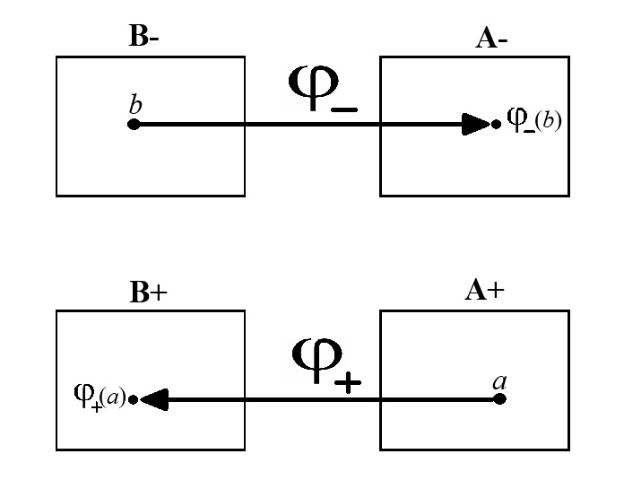
Notice that in defining a morphism from to , we automatically get a dual morphism from to .
Defining a relation for a specific cardinal is already cumbersome. Moreover, it is not always clear how to define a relation whose dual corresponds to a different cardinal. So one might wonder why we choose to work within such a category. The reason lies in the following, simple but powerful, theorem.
Theorem 2.9.
If there exists a morphism then and .
Proof.
The latter inequality follows immediately after applying the former inequality to the dual morphism , so we will only prove the first.
Suppose is a morphism from to . Let be a cofinal set with cardinality . Since , it suffices to show that is cofinal in . To this end, let be arbitrary and suppose , for some . By the definition of a morphism, . ∎
Definition 2.10.
Given a relation , we can define a corresponding sigma-relation,
means that for every . represents the least cardinality of a solution set such that any countable set of problems can be solved by at least one .
It is always the case that , as a morphism can be trivially constructed by allowing to be the function that associates elements with any countable set including within it and letting be the identity. For many cardinal characteristics, it remains an open question as to whether or not this inequality can be made strict.
Example 2.11.
Notice . Then and . Whether or not is consistent with ZFC is an open problem.
From the above examples, we learn that norms of relations can represent certain cardinal characteristics and from the preceding theorem, we learn that morphisms between relations induce inequalities between these norms. Since our goal is to study inequalities among cardinal characteristics, it is unsurprising that much of this thesis will focus on explicitly constructing morphisms between various relations. Before moving on to more general categorical questions we will give one more useful result regarding morphisms.
Theorem 2.12.
Suppose and are two relations and is a cardinal.
-
(1)
if and only if there exists a morphism from to .
-
(2)
If , then there exists a morphism from to .
-
(3)
If , then there exists a morphism from to .
-
(4)
If , then there exists a morphism from to .
Proof.
-
(1)
We first construct a morphism . Assuming that , we can let surject onto a cofinal set of solutions within . For an arbitrary we will let be equal to some , such that is a solution for . To verify this is a morphism, we must check that implies . This is immediate by the construction of . The other direction is obvious because of Theorem 2.9.
-
(2)
Let be an injection. For any , we can define the set . Since , there exists at least one which is not solved by any element of . We will let be the function associating each with some corresponding . Assuming that , for some , we get .
-
(3)
If we apply (2) to the dual relation , we get a morphism from into
-
(4)
From (2) we get a morphism and from (3) we get a morphism . Then , is a morphism from to . The fact that we can compose morphisms is proved in Proposition 2.13.
∎
2.2. The Category
Proposition 2.13.
is a category.
Proof.
-
(1)
Identity Morphisms: Let be arbitrary. We will define the identity morphism as where is the identity map on , and is the identity map on . For any and , if , then . Hence, is a morphism.
-
(2)
Composition of Morphisms: Let and . We define and . Suppose , meaning . Since is a morphism, we get , and because is a morphism, . Hence, , and so is a morphism.
-
(3)
Associativity of Composition: This follows from the associativity of set functions.
∎
We can also ask whether or not contains zero objects. The answer is a resounding “no.” In fact, contains neither initial nor final objects.
Proposition 2.14.
There are no zero objects in
Proof.
Suppose, for the sake of contradiction, that was initial. Let be a set of strictly greater cardinality than and define the relation . Since is initial, there exists a morphism . By Theorem 2.9, this means that .
If we instead assumed that was final, this would imply there is a morphism , for any arbitrary relation . By applying the above argument to we end up with the same contradiction. ∎
Although lacks zero objects, there is still structure to be found. In particular, we can define finite products and co-products.
Definition 2.15.
The product of two relations is defined as the relation . means that if and , then . If instead and , then means . The coproduct is defined as .
Theorem 2.16.
-
(1)
-
(2)
Proof.
We will only prove (1) as (2) can be proven with a dual argument. By definition, a cofinal set contains a solution for every problem . By associating each pair with its corresponding element , we see that . Likewise, by associating each pair with its corresponding element , we get that .
To show that , we separately consider the case where both and are finite and the case where at least one of the two is infinite. Starting with the infinite case, let be a cofinal set with and let be a cofinal set with . Fix and and define:
By the fact that is a solution set for and properties of infinite cardinal arithmetic,
If both and are finite, let and . Without loss of generality, assume that . Define :
If is a problem, then there must be some such that . If then, is a solution. If then is a solution. If is a problem, then is a solution. This shows that is a solution set for . Thus,
∎
Beyond the product and co-product, there are several other ways we can combine two relations.
Definition 2.17.
For two relations and :
-
(1)
The conjunction is the relation , where means and
-
(2)
The sequential composition is the relation . Where means and .
-
(3)
The dual sequential composition is the relation .
As shown below, properties analogous to Theorem 2.16 remain true for relations defined above. The proofs of which are similar to the argument given in Theorem 2.16 and are therefore omitted.
Theorem 2.18.
-
(1)
-
(2)
-
(3)
In the infinite case, maximums and products are the same. For (1) this means that and for (2) this means that .
3. Cichoń’s Diagram
Cichoń’s diagram is a crucial tool in the study of cardinal characteristics of the continuum. It elegantly organizes several important cardinal invariants that measure different properties of the real line. As depicted here, the diagram is backward in comparison to its traditional orientation. That is, all the below arrows are reversed. Usually, an arrow from one cardinal characteristic to another characteristic represents the fact that . For our purposes, we take an arrow from to to mean that there exists a morphism . Where and represent relations whose norms are and , respectively. Thus, the reason we reverse arrows boils down to Theorem 2.9.
One of the primary reasons Cichoń’s diagram is significant is because of its ability to unify seemingly separate areas within set theory. Cardinal characteristics related to Lebesgue measure, such as and , find their counterparts in the realm of Baire category through invariants like and . This unification reveals connections between measure-theoretic and topological properties of . Moreover, Cichoń’s diagram plays a role in independence results. Different models of set theory, achieved through various forcing extensions or by adopting alternative axioms beyond ZFC, can result in distinct versions of the diagram in which the relative sizes of the cardinal characteristics differ [11]. However, the version presented here represents the standard configuration within ZFC. This canonical diagram captures the foundational ZFC-provable inequalities and serves as a baseline for our analysis.
The main objective of this section will be to explicitly construct each morphism presented in Figure 2. To achieve this, we will start by formally defining each of the depicted cardinal characteristics. Following these definitions, we will introduce relations whose norms correspond to each defined cardinal. After all of this, we will construct the relevant morphisms.
3.1. Bounding and Dominating
As defined in examples 2.4 and 2.5, the two cardinals from Cichoń’s diagram that we start with are and .
Theorem 3.1.
.
Proof.
By Example 2.4, we associate with the norm of the relation and with the norm of the dual relation .
Let both be the identity function. Then implies Since domination is antisymmetric, . ∎
After having proved Theorem 3.1, we need to establish that is uncountable. Doing so within requires a morphism from into a relation whose norm is . The most natural candidate for such a relation would be something like . We now show that no such morphism exists. In fact no relation with will work.
Proposition 3.2.
Let be a relation such that . If is a morphism, then .
Proof.
For contradiction, suppose Define . Since is not a dominating family, let be a function not dominated by any element of . By the definition of a morphism, for every , . This implies . By contradiction, is a dominating family. But this is impossible since . ∎
It should be noted that we can easily get the above result by considering the dual morphism , but the details of this proof will serve as an interesting comparison later on with Proposition 4.1 and Theorem 4.5. Moreover, Proposition 3.2 can be generalized to similar relations with norm . For example, the alternate construction given in Example 2.5 will also fail because there are morphisms to and from it and the standard relation for . Although it may be possible to construct a relation and a corresponding morphism that work in this scenario, it is likely difficult. As such a relation could not have a morphism from the standard witnesses for into it and its problem set must have strictly greater cardinality than . This is all to say that giving a direct proof is much easier.
Proposition 3.3.
Proof.
Let be an arbitrary countable family of functions. For every define the function as:
Since dominates each , we can say that at least one function dominates any countable family of functions. ∎
3.2. Ideals
Definition 3.4.
Given a set , an ideal on is a nonempty subset of such that:
-
(1)
If and , then .
-
(2)
If , then .
-
(3)
, ( is proper).
It should be clear that ideals are dual to filters. Less obviously, recall that can be transformed into a commutative ring by defining addition with symmetric differences, multiplication by intersections, and letting the additive identity be the empty set. Under these conditions is a Boolean ring, meaning that each of its elements is idempotent under multiplication. In this context, subsets conforming to the conditions of Definition 3.4 are ideals in the ring theoretic sense.
Definition 3.5.
Let be a proper ideal of subsets of a set which contains all of its singletons.
-
(1)
The additivity of , , is the smallest number of sets in with union not in . Formally,
-
(2)
The covering number of , , is the smallest number of sets in with union . Formally,
-
(3)
The uniformity of , , is the smallest cardinality of any subset of not in . Formally,
-
(4)
The cofinality of , , is the smallest cardinality of a such that each element of is a subset of an element of . Such a is called a basis for . Formally,
Define, and . Then, , , , and .
When the ideal is generated by first category (meager) sets, we denote it as , for “Baire.” Likewise, if the ideal is generated by Lebesgue measure zero sets, we denote it as , for “Lebesgue.” Additionally, if we take our underlying set to be different versions of the continuum (, , , etc), we will not notationally distinguish them. Each version of all of the relations admits morphisms in both directions, making them essentially equivalent. With this all in mind, we are now ready to give our first result about cardinal characteristics related to ideals.
Theorem 3.6.
There exist morphisms:
-
(1)
.
-
(2)
.
-
(3)
.
-
(4)
.
Proof.
We want to construct morphisms:
To construct , let map any to the set and let be the identity. For some , if then .
To construct first let be arbitrary. Since is proper, we can choose arbitrarily. Define and let be the identity. If then , since .
By Theorem 2.9, taking the duals of and finishes the proof. ∎
Corollary 3.7.
Theorem 3.6 also implies the existence of several other morphisms but, since our goal is to create Cichoń’s diagram, we will take these to be superfluous.
3.3. Baire Characteristics
Our next objective is to construct morphisms witnessing the inequalities and To do so we must first define the concepts of “chopped reals” and “matching.” This will allow us to prove two lemmas which, in turn, let us construct alternate relations witnessing and . Given these alternate relations, we can construct our desired morphisms.
Definition 3.8.
A chopped real is a pair , where and is an interval partition of . We write “” for the set of chopped reals. We say a real matches a chopped real if for infinitely many .
Lemma 3.9.
is meager if and only if there is a chopped real that no member of matches.
Proof.
For , the set of all reals matching a chopped real is:
In the product topology on , basic open sets are families which are fixed for finitely many coordinates. Therefore, each set is open. To show that is dense, consider an open set defined by fixing values on some finite set . For some , let be the maximum element of . Let be a function fulfilling the open set conditions on and require that , for some . By construction, . Since was arbitrary, this shows is dense. Thus, is a countable intersection of dense open sets. By the Baire Category Theorem, is meager and so is meager.
A nowhere dense set is such that for every finite binary sequence , there exists a finite extension , such that no further extends . To prove the other direction, first assume that is meager. Let be a countable sequence of nowhere-dense sets which cover . For each , it can be assumed that . Our goal is to construct a chopped real , such that for each and , . If we can do this, since any is such that for some and , we would have that for all , i.e. .
To construct such a chopped real we use recursion. Assume that and are defined for each . If is the right endpoint of , we can let enumerate all length binary sequences. We want to construct using non-overlapping sub-intervals , so that . Since is nowhere dense, there is some function which extends onto , so that none of further extends . Define as . Likewise, there is some function which extends onto , so that none of further extends . Define as , and so on. By recursively constructing in this way, after steps we will have defined both and . Let and be arbitrary. By construction , for some and so . Since , . ∎
Lemma 3.10.
if and only if for all but finitely many intervals there exists an interval such that and .
Proof.
First assume that . For contradiction, suppose that there are infinitely many such that for each , implies . Let be an infinite set of such and let agree with on each . Moreover, for each , define .
Since agrees with on all of , it has to agree with on infinitely many . Thus, and by assumption . Define the set , which is infinite because . Notice that each is a subset of . If , by construction . But, this contradicts the fact that . Thus, for each there exists an such that . So given a , by assumption but, since , .
To prove the reverse direction assume that . Let and suppose that for all but finitely many , there exists a such that and . Define and observe that is infinite since . By assumption, for each of the infinitely many , there are infinitely many with , such that . Consequently, there are infinitely many such that , which implies that . ∎
Before we utilize the above two lemmas to construct an alternate witness for , we must first define a binary relation for this witness. To this end, we give the following definition.
Definition 3.11.
A chopped real engulfs another chopped real if,
In our construction for an alternate witness to will follow naturally to define an alternate witness for . So we will construct both in the following lemma.
Lemma 3.12.
There exist morphisms
-
(1)
-
(2)
-
(3)
-
(4)
Proof.
-
(1)
As in Lemma 3.9, define as . Define as , where is a chopped real such that no member of matches it. Such a chopped real exists because of Lemma 3.9. Assume that for an arbitrary chopped real and . We want to show that is engulfed by . If then , which implies . By contraposition, if then . By definition, is engulfed by .
-
(2)
As above, define as for any Define as for any . If we assume that is engulfed by , Lemma 3.10 says . If then . This implies that , i.e. .
-
(3)
Let be the identity and for any let equal . If , then does not match .
-
(4)
Let be the identity and let be defined as . If does not match , then .
∎
With the two alternate relations in mind, we are finally ready to prove the inequalities we initially sought.
Theorem 3.13.
and .
Proof.
We first produce a morphism from into . For an arbitrary , define as . Define as . Assume that is engulfed by some . By Lemma 3.10, this implies that must dominate .
We now construct a morphism from into . Considering the duals of this morphism and the above morphism will complete the proof. By taking both and to be the identity, we obtain a morphism between and the relation For , is eventually different than means that for all but finitely many , . Then, Lemma 3.12 implies that constructing a morphism and composing it with the above morphism completes the proof. To this end, let be the identity and assume that is eventually different than . Let , defining implies that cannot match . If it did, by the construction of , for all but finitely many , . Thus, defines a morphism from to . ∎
It has been proven [2] that and . So technically, the identity morphism from into completed the latter half of the proof.
3.4. Lebesgue Characteristics
Now that we have constructed morphisms between each of the category relations and measure relations we defined, it only remains to bridge the gap between measure and category.
Theorem 3.14.
and .
Proof.
Our goal is to find a suitable relation , such that we can construct morphisms , from the relation into and , from into Then and witness our desired inequalities. To this end, let be an interval partition of whose interval has elements. Take to mean that there are infinitely many such that . Moreover, define
Before we construct the morphisms, we will prove is co-meager and measure zero. The claim that is co-meager follows directly from Lemma 3.9, since none of matches . To prove has measure zero, for every , define and notice . Since open sets fix a finite number of coordinates, we can place a probability measure on based on a given finite sequence. Concretely, if we specify bits of a sequence, the probability that any sequence agrees with this partial assignment is . Extending this to infinitely many coordinates gives the full probability measure on . In our case, a single interval has length and the set of all sequences that match on has measure . Recalling the definition of , this implies . By continuity of the measure,
.
Let both and be the identity on . If we let and , we get our desired morphisms. ∎
It only remains for us to prove there exists a morphism witnessing the inequalities and . We start with the following lemma.
Lemma 3.15.
and
Proof.
and is already implied by Theorem 3.6 and Theorem 3.13. So if we can exhibit a morphism
by Theorem 2.18 and Lemma 3.12, we will have proved the lemma. Since , we can allow to be the identity. To define we require two maps and . We let be the identity and define as follows. For each and each , if does not match , let be arbitrary. If does match , let be such that each of its blocks contains exactly one of the infinitely many intervals where and agree.
Define and let be arbitrary. We require that if and is dominated by , then is engulfed by . This implication trivially holds if does not match , so we assume it does. By construction, within each block there exists an interval for which . Since dominates , for all but finitely many there exists some such that . Thus, for all of these , we have , where . By Lemma 3.10, is engulfed by ∎
Before we construct our desired morphism, we need to give an alternate characterization of , first discovered in [1]. To this end, we give the following definition.
Definition 3.16.
A slalom is a function such that for each , has cardinality . We say that a function , goes through a slalom if, for all but finitely many , . We denote as the set of all slaloms.
Proposition 3.17.
.
The proof of this theorem can be found in [1]. There it is proven that is the least cardinality of any family of functions such that there is no single slalom through which all of the members of it go. This is equivalent to the above norm condition.
Theorem 3.18.
and .
Proof.
Given Lemma 3.15, it suffices to exhibit morphisms witnessing and . Since , by the universal property of co-products, this would show that there exists a unique morphism witnessing . The dual of this morphism will witness .
We first construct a morphism . Let map a slalom to the function , where , for every . For some , if we suppose that , then there are infinitely many such that . By construction of , there are infinitely many such that, . Thus, defining as the identity suffices.
The remark at the end of Theorem 3.13, states that is equivalent to the relation The most straightforward way to produce a morphism is through . But, because we have not justified the equality of with , we refer to the proof given in chapter 5 of [3] for this morphism. Although the morphism is not given explicitly in the proof, it is not difficult to implicitly draw it out. ∎
4. More Cardinal Characteristics
Although Cichoń’s diagram is a useful classification tool for cardinal characteristics related to category and measure, many more cardinal characteristics exist beyond the ones mentioned in the previous section. For many of these cardinal characteristics , apart from the trivial relation , it is often challenging to define a relation that is easy to work with. The purpose of the category is to simplify the study of cardinal characteristics of the continuum. Therefore, if incorporating a certain cardinal characteristic or inequality into this framework complicates the proofs without yielding any new insights, then its inclusion is unnecessary. In this section, we shift our attention towards a subset of cardinal characteristics, beyond the ones mentioned in Cichoń’s diagram, which are easily amenable to the framework.
4.1. Splitting and Reaping
As defined in Example 2.6, the first two cardinal characteristics we will discuss are and .
When we first introduced and , we sought to construct a morphism from a relation whose norm is into a relation whose norm is . However, as indicated by Proposition 3.2, such a morphism would necessitate a very non-standard witness for , so we instead opted for a direct proof. In a nearly identical way, we now show that attempting to build a morphism from a relation with norm into a relation with norm necessitates a witness for which is just as non-standard.
Proposition 4.1.
Let be a relation such that . If is a morphism, then .
Proof.
For contradiction, suppose Define . Since is not a reaping family, let split every element of . By the definition of a morphism, for every , . This implies . By contradiction, is a reaping family. But this is impossible since . ∎
This proof is nearly identical to Proposition 3.2 and for similar reasons as with , we instead opt for a direct proof to show that . Also, as in Proposition 3.2, we can just as easily prove Proposition 4.1 by considering the dual morphism .
Theorem 4.2.
.
Proof.
Let , be a countable family of infinite sets. We will show that is not a splitting family. Define and let . For each , assume that are infinite sets such that and are distinct elements with each . If is infinite let , otherwise let . In either case choose distinct from . By induction, the set is infinite. Moreover, for every the set is a subset of and either or . Thus for each , either or is finite. ∎
The cardinal characteristics and share many similarities with and , respectively. In fact, it is consistent with ZFC that and [9]. The following morphism succinctly produces the known inequalities between and .
Theorem 4.3.
and
Proof.
We seek a morphism .
Define as , where is the unique strictly increasing bijection from to .
Let be defined as , where:
We assume, without loss of generality, that is increasing. If , let be the point past which dominates . For every we get that :
This implies that if and only if is even. So when is even is infinite. Otherwise, if is odd, and so is infinite. By definition, splits . ∎
We can also relate and to category and measure.
Theorem 4.4.
Proof.
For any let . Before moving forward, notice that the standard product topology on can be aligned with the standard product topology on . This is done by associating each with the set , where is the characteristic function for . With this in mind, we claim that is meager and of measure zero. To see this notice that
For every , both and are meager and measure zero, which implies is meager and measure zero.
To see why is measure zero, consider the event that any is also in . Since each such event occurs with probability independently, and is infinite, the sum of these probabilities diverges. By the second Borel–Cantelli lemma [4], it follows that almost every will have infinitely many elements from . Thus, the probability that contains only finitely many elements from is zero. We can make a similar argument in the case of .
To show that is meager, observe that since is infinite, we can choose additional coordinates in (beyond the finitely many fixed ones) and force those coordinates to be in . This ensures meets in more than points. Hence, we can find a smaller open set disjoint from , showing that this set is nowhere dense. A countable union of nowhere dense sets is meager, so is meager. We can again make a similar argument in the case of .
Let be the identity and let . Then can be used as a morphism from into and from into . ∎
4.2. Ramsey-like Characteristics
Ramsey’s theorem states that for any , for any , and any coloring , there exists an infinite subset such that is homogeneous for . As defined in Example 2.7, the homogeneity number, denoted , is the Ramsey-theoretic analog of . The partition number, denoted , is the Ramsey-theoretic analog of .
Our first task will be to prove that . We opt for a direct proof of this fact for similar reasons as with and .
Theorem 4.5.
Proof.
We need to prove that for any countable family of -colorings, there exists an infinite set which is almost homogeneous for all of it. Instead, we prove a stronger analog of this statement. In particular, we show that for any family of colorings , where and are countable sets of integers, there is an which is almost homogeneous for the entire family.
We go by induction. Let be an infinite set homogeneous for ; exists by Ramsey’s theorem. Assume that are defined up to some and that are homogeneous for each of them respectively. Let and . Another application of Ramsey’s theorem ensures there is an infinite subset of which is homogeneous for , call it . Then, the infinite set is almost homogeneous for each coloring in the family. ∎
The next two propositions seek to solidify the comparisons among and . After this, we prove that there exist morphisms witnessing the inequalities and . The result actually holds for every , but we will only consider when . This is because (1) the proofs for arbitrary are practically identical and (2) the following proposition establishes that the case of suffices to prove all relevant inequalities for .
Proposition 4.6.
For integers , and .
Proof.
It suffices to produce a morphism .
Let send any coloring to the coloring , defined as . Let be the identity. If is almost homogeneous for some , restricting to coordinates remains constant after removing a finite set. ∎
Proposition 4.7.
and .
Proof.
To prove this theorem we exhibit morphisms to and from and .
First we produce a morphism . Let , the set of all for which . Let be the identity. If does not split some , by definition or is finite. If is finite then is almost always . If is finite then is almost always . In any instance, is almost homogeneous for .
For the reverse morphism let send any to its characteristic coloring. Concretely, let where
Let be the identity. If is almost homogeneous for some , then the restriction of to is either almost always or , but not both. For contradiction, assume that splits . Since is infinite, is almost homogeneous for . But since is infinite, is almost homogeneous for . By contradiction, does not split . ∎
Theorem 4.8.
and
Proof.
It suffices to construct a morphism from . This is because composing the morphisms given in Proposition 4.6 and Proposition 4.7 gives a morphism witnessing . It is also possible to do this directly [9].
For a strictly increasing function , let be defined as where,
For any , define as , where is the unique strictly increasing bijection from into . Suppose is almost homogeneous for . If for almost every , then every pair must lie within the same interval. This is impossible as is infinite and such an interval would be finite. So it must be that for almost every . In the words, for almost every pair , there is no interval that both and are elements of. Notice that the intervals form a partition of and the least interval that could lie in is . So even in the worst case, . Likewise, the least interval that could lie in is and this still implies that . Continuing in this way, we see that past , . Thus, is dominated by . ∎
The above inequality can be strengthened into an equality if we consider instead of . Particularly, for , it can be shown that there is a morphism witnessing and . Since , the above theorem implies that and . Notice that in requiring instead of we fail to get a perfectly dual inequality for . Fortunately, it still is the case that . We just have to construct an extra morphism to prove it. If we attempted to construct the morphism witnessing , Definiton 2.17 would tell us it must go from into . This would amount to producing a morphism
where requires three separate conditions to be met. This would be inelegant, to say the least. Alternatively, we provide a direct proof of this result and note that the above morphism can be found implicitly within the argument.
Theorem 4.9.
For , and .
Proof.
We first prove . To do this, by Theorem 4.8, it suffices to show To this end, we employ the following argument due to Brendle [5].
Let have property. This means that for any -coloring there exists which is almost homogeneous for Given a countable family of maps define for each an infinite binary sequence For , define a -coloring by
Let be almost homogeneous for By removing finitely many elements, we obtain an infinite on which is homogeneous in (a similar argument works for ). As increases, can only increase. Increasing here means that goes from to . But once changes from to , it must remain as . Otherwise, the lexicographical ordering fails. Once stabilizes, increases and then stabilizes, after this increases and stabilizes, and so on. This shows that the family is almost homogeneous on and thus on .
We now have to prove that . To do this we will construct a set with cardinality and show that it has property.
Let be a dominating family with a cardinality of . Let be a -reaping family with a cardinality of . Then for each , we can construct a reaping family .
To see why this is possible, notice that we can take to be the set . Under this definition, if is not reaping then we can assume that there is some which splits each of its elements. This would imply that splits , for every . In other words, would have to split all of , which is a contradiction.
For every , , and , we let be such that , for any within . The family , of each , has cardinality at most .
Let be an arbitrary -coloring. For each we can define the function as . Since is -reaping, we can find some set for which each is almost homogeneous on. On , we can say for every . Here, indicates the point past which is homogeneous and indicates the color in which is almost homogeneous. Since is reaping, there is some such that is almost constant on it, say for every . Moreover, let dominate past the point .
By the construction of , for , . Thus, , i.e. is almost constant on . ∎
4.3. The Lower Topology
We now introduce the final two cardinal characteristics included in this thesis. To do this, we first define the “lower topology” on . In the lower topology, open sets are defined as families which are closed under almost subsets. Being closed under almost subsets means that if and there is a , such that is finite, then . It can be shown that for a family , being dense is equivalent to every infinite set having a subset with . We let “”, denote the set of all dense-open sets within the lower topology.
The first cardinal characteristic we define related to the lower topology is “”, the “shattering number”, also referred to as the “distributivity” number. is the least number of dense-open sets with an empty intersection. Equivalently, we define .
The second cardinal characteristic related to the lower topology is , the “groupwise-dense” number. We say a family is groupwise dense if it is open within the lower topology and for every interval partition , there exists an infinite set of intervals such that . is the least number of groupwise dense families having empty intersection. Equivalently, we define , where denotes the set of all groupwise dense subsets.
Notice that and are not duals of one and other. We will prove that both the duals for and have cardinality . To this end, we first introduce the idea of “almost disjoint-ness” and state a proposition relating to it. We say two sets are almost disjoint if is finite. Moreover, a family of pairwise almost disjoint infinite sets is called an “almost disjoint family.” It should be noted that the least cardinality of a maximal almost disjoint (MAD) family, defines a cardinal characteristic of its own, —the “almost disjoint number.” It can be shown that but, since defining a relation witnessing this is not obvious to me, we will forego further discussion about . Instead, we continue with the following proposition and lemma.
Proposition 4.10.
There exists a maximal almost disjoint family of cardinality .
Proof.
Let denote the set of all finite binary strings. A branch of is a function . Since is in bijection with , the set of all branches of has cardinality . For each , let be the set of all initial segments of . If are distinct then there must be some such that . This implies is finite, thus the set is almost disjoint with cardinality . By Teichmüller’s principle, we can extend to a maximal almost disjoint family ∎
In addition to being useful for the theorem we want to prove, Proposition 4.10 also shows that is well defined.
Lemma 4.11.
Let be a MAD family and let . For any distinct elements either or is finite if and only if there exists an element such that is finite.
Proof.
Suppose first that for any two distinct sets either or is finite. It cannot be the case that every has a finite intersection with . If this were the case, then would be a MAD family containing , which contradicts maximality. Thus let, have infinite intersection with . By assumption for every , is finite and for each of these , is finite. If is infinite then would not be MAD, which proves is finite.
For the other direction suppose there is an such that is finite. Since is almost disjoint, every must have a finite intersection with . ∎
Theorem 4.12.
.
Proof.
We will only prove , as the proof for is almost exactly the same. Since , it suffices to prove .
Suppose for contradiction that is the subset of witnessing . Our goal is to construct a dense-open set such that no element of is in the set. To this end, let be a MAD family and define
If then there is some such that is finite. If for some , is finite, then is finite. This shows that is open. To show density, let be a set not in (the case where is trivial.) Since is MAD, there is a such that is infinite. Then and , proving density.
If is any arbitrary element, we want to show that . For contradiction suppose that , then there is some such that is finite. By being MAD, if then for any distinct either or is finite. By Lemma 4.11 this implies there exists some such that is finite, which means that . By contradiction, no element of is an element of . ∎
In light of Theorem 4.12, Theorem 4.8, and Proposition 4.7, the dual realization of the theorem below proves that most of the cardinal characteristics discussed in the thesis have cardinality less than or equal to . The ones not included are those not mapped to by . In addition, the theorem below shows that functions as a lower bound for all the cardinals discussed in this section.
Theorem 4.13.
Proof.
We construct a morphism
Let be the identity function. For any 2-coloring let be the family of all infinite sets which are almost homogeneous for . If is an arbitrary infinite set that is not almost homogeneous , then .
We must now verify that is a dense-open subset. Density follows directly from Ramsey’s theorem. To verify that is open, observe that adding finitely many elements to an almost homogeneous set results in another almost homogeneous set. ∎
Theorem 4.14.
Proof.
We can construct morphism , by letting both and be the identity. The only non-trivial aspect is showing that any groupwise dense set is dense-open. By definition, any groupwise dense set is open. To show density, let be an arbitrary groupwise dense family. For any , let be such that each interval contains at least one element from . By closure under almost subsets, the union over each gives an infinite subset of which is in .
To produce a morphism , we let associate with the function enumerating it. Assume that and let , defined as:
If, for contradiction, we supposed that , this would imply that there are infinitely many such that . If is the point past which dominates , then for each , . This implies that for all but finitely many , . ∎
References
- [1] Tomek Bartoszyński. Additivity of measure implies additivity of category. Transactions of the American Mathematical Society, 281:209–213, 1984.
- [2] Tomek Bartoszyński. Combinatorial aspects of measure and category. Fundamenta Mathematicae, 127:225–239, 1987.
- [3] Andreas Blass. Combinatorial cardinal characteristics of the continuum. In Matthew Foreman and Akihiro Kanamori, editors, Handbook of Set Theory, pages 395–491. Springer, 2010.
- [4] Émile Borel. Les probabilités dénombrables et leurs applications arithmétiques. Rendiconti del Circolo Matematico di Palermo (2), 27:247–271, 1909.
- [5] Jörg Brendle. Strolling through paradise. Fundamenta Mathematicae, 148:1–25, 1995.
- [6] Georg Cantor. über eine eigenschaft des inbegriffes aller reellen algebraischen zahlen. Journal für die reine und angewandte Mathematik (Crelle), 77:258–262, 1874.
- [7] Paul J. Cohen. The independence of the continuum hypothesis. Proceedings of the National Academy of Sciences of the United States of America, 51(7):1146–1153, 1963.
- [8] Kurt Gödel. Über formal unentscheidbare sätze der principia mathematica und verwandter systeme i. Monatshefte für Mathematik und Physik, 38(1):173–198, 1938.
- [9] Lorenz J. Halbeisen. Combinatorial Set Theory: With a Gentle Introduction to Forcing. Springer, Berlin, Heidelberg, 1st edition, 2012.
- [10] J. D. Monk. Continuum cardinals, April 2014.
- [11] Corey Bacal Switzer. Alternative cichoń diagrams and forcing axioms compatible with ch, 2020.
- [12] Peter Vojtáš. Generalized galois-tukey connections between explicit relations on classical objects of real analysis. In Haim Judah, editor, Set Theory of the Reals, volume 6, pages 619–643. American Mathematical Society, Providence, 1993.